Contents lists available at SciVerse ScienceDirect
Physica A
journal homepage: www.elsevier.com/locate/physa
Equivalent continuous and discrete realizations of Lévyflights: A model of one-dimensional motion of an inertialparticleIhor Lubashevsky ∗
University of Aizu, Ikki-machi, Aizu-Wakamatsu, Fukushima 965-8560, Japan
a r t i c l e i n f o
Article history:Received 30 September 2012Received in revised form 8 January 2013Available online 8 February 2013
Keywords:Lévy flightsNonlinear Markovian processesRandommotion trajectoriesExtreme fluctuationsPower-law heavy tailsTime scaling lawContinuous time random walks
a b s t r a c t
The paper is devoted to the relationship between the continuous Markovian descriptionof Lévy flights developed previously (see, e.g., I.A. Lubashevsky, Truncated Lévy flights andgeneralized Cauchy processes, Eur. Phys. J. B 82 (2011) 189–195 and references therein)and their equivalent representation in terms of discrete steps of awandering particle, a cer-tain generalization of continuous time random walks. To simplify understanding the keypoints of the technique to be created, our consideration is confined to the one-dimensionalmodel for continuous random motion of a particle with inertia. Its dynamics governed bystochastic self-acceleration is described asmotion on the phase plane x, v comprising theposition x and velocity v = dx/dt of the given particle. A notion of random walks inside acertain neighborhoodL of the line v = 0 (the x-axis) and outside it is developed. It enablesus to represent a continuous trajectory of particle motion on the plane x, v as a collectionof the corresponding discrete steps. Each of these steps matches one complete fragment ofthe velocity fluctuations originating and terminating at the ‘‘boundary’’ of L. As demon-strated, the characteristic length of particle spatial displacement is mainly determined byvelocity fluctuations with large amplitude, which endows the derived randomwalks alongthe x-axis with the characteristic properties of Lévy flights. Using the developed classifica-tion of random trajectories a certain parameter-free core stochastic process is constructed.Its peculiarity is that all the characteristics of Lévy flights similar to the exponent of theLévy scaling law are no more than the parameters of the corresponding transformationfrom the particle velocity v to the related variable of the core process. In this way the pre-viously found validity of the continuousMarkovianmodel for all the regimes of Lévy flightsis explained. Based on the obtained results an efficient ‘‘single-peak’’ approximation is con-structed. In particular, it enables us to calculate the basic characteristics of Lévy flights us-ing the probabilistic properties of extreme velocity fluctuations and the shape of the mostprobable trajectory of particle motion within such extreme fluctuations.
During the last two decades there has been a great deal of research into Lévy type stochastic processes in various systems(for a review see, e.g., Ref. [1]). According to the accepted classification of the Lévy type transport phenomena [1], Lévyflights are Markovian random walks characterized by the divergence of the second moment of walker displacement x(t),
2324 I. Lubashevsky / Physica A 392 (2013) 2323–2346
i.e., ⟨[x(t)]2⟩ → ∞ for any time scale t . It is caused by a power-law asymptotics of the distribution function P (x, t). Forexample, in the one-dimensional case this distribution function exhibits the asymptotic behavior P (x, t) ∼ [x(t)]α/x1+αfor x ≫ x(t), where x(t) is the characteristic length of the walker displacements during the time interval t and theexponent α belongs to the interval 0 < α < 2. The time dependence of the quantity x(t) obeys the scaling lawx(t) ∝ t1/α . Lévy flights are met, for instance, in the motion of tracer particles in turbulent flows [2], the diffusionof particles in random media [3], human travel behavior and spreading of epidemics [4], or economic time series infinance [5].
As far as the developed techniques of modeling such stochastic processes are concerned, worthy of mention are, inparticular, the Langevin equation with Lévy noise (see, e.g., Ref. [6]) and the corresponding Fokker–Planck equations [7–10], the description of anomalous diffusion with power-law distributions of spatial and temporal steps [11,12], Lévyflights in heterogeneous media [13–17] and in external fields [18,19], constructing the Fokker–Planck equation for Lévytype processes in nonhomogeneous media [20–22], first passage time analysis and escaping problem for Lévy flights[23–33].
One of the widely used approaches to coping with Lévy flights, especially in complex environment, is the so-calledcontinuous time random walks (CTRW) [34,35]. It models, in particular, a general class of Lévy type stochastic processesdescribed by the fractional Fokker–Planck equation [36]. Its pivot point is the representation of a stochastic process at handas a collection of random jumps (steps) δx, δt of a wandering particle in space and time as well. In the frameworks of thecoupled CTRW the particle is assumed to move uniformly along a straight line connecting the initial and terminal points ofone step. In this case the discrete collection of steps is converted into a continuous trajectory and the velocity v = δx/δt ofmotion within one step is introduced. As a result, the given stochastic process is described by the probabilistic properties,e.g., of the collection of random variables v, δt. A more detailed description of particle motion lies beyond the CTRWmodel. Unfortunately, for Lévy flights fine details of the particle motion within one step can be important especially inheterogeneous media or systems with boundaries because of the divergence of the moment ⟨[δx(δt)]2⟩. Broadly speaking,it is due to a Lévy particle being able to jump over a long distance during a short time. The fact that Lévy flights can exhibitnontrivial properties on scales of one step was demonstrated in Ref. [30] studied the first passage time problem for Lévyflights based on the leapover statistics.
Previously a new approach to tackling this problem was proposed [37–40]. It is based on the following nonlinearstochastic differential equation with white noise ξ(t)
τdvdt
= −λv +
τ(v2a + v2)ξ(t) (1)
governing random motion of a particle wandering, e.g., in the one-dimensional space Rx. Here v = dx/dt is the particlevelocity, the time scale τ characterizes the delay in variations of the particle velocity which is caused by the particle inertia,λ is a dimensionless friction coefficient. The parameter va quantifies the relative contribution of the additive componentξa(t) of the Langevin force with respect to the multiplicative one vξm(t)which are combined within one term
vaξa(t)+ vξm(t) ⇒
(v2a + v2)ξ(t). (2)
Here we have not specified the type of the stochastic differential equation (1) because in the given case all the typesare interrelated via the renormalization of the friction coefficient λ. It should be noted that models similar to Eq. (1)within replacement (2) can be classified as the generalized Cauchy stochastic process [41] and has been employed tostudy stochastic behavior of various nonequilibrium systems, in particular, lasers [42], on–off intermittency [43], economicactivity [44], passive scalar field advected by fluid [45], etc.
Model (1) generates continuous Markovian trajectories obeying the Lévy statistics on time scales t ≫ τ [37–39]. Usinga special singular perturbation technique [38] it was rigorously proved for the superdiffusive regime matching 1 < α < 2[37,38] and also verified numerically for the quasiballistic (α = 1) and superballistic (0 < α < 1) regimes [39]. Moreover,the main expressions obtained for the distribution function P (x, t) and the scaling law x(t) within the interval 1 < α < 2turn out to hold also for the whole region 0 < α < 2 [39]. After its generalization [40] model (1) generates truncated Lévyflights as well.
The given approach can be regarded as a continuous Markovian realization of Lévy flights. Indeed, it is possible to choosethe system parameters in such a way that, on one hand, the ‘‘microscopic’’ time scale τ be equal to an arbitrary small valuegiven beforehand and, on the other hand, the system behavior remain unchanged on scales t ≫ τ [37,38]. The goal of thispaper is to elucidate the fundamental features of this approach, to explain the found validity ofmodel (1) for describing Lévyflights of all the regimes, and to construct a certain generalization of the continuous time randomwalks that admits a ratherfine representation of the particle motion within one step. The latter feature will demonstrate us a way to overcome thebasic drawback of the CTRW model, it appeals to different mechanisms in modeling the particle motion within individualsteps and the relative orientation of neighboring steps.
I. Lubashevsky / Physica A 392 (2013) 2323–2346 2325
2. Continuous Markov model of Lévy flights
2.1. Model
Following [37,39,40] let us consider random walks x(t) of an inertial particle wandering in the one-dimensional spaceRx whose velocity v = dx/dt is governed by the following stochastic differential equationwritten in the dimensionless form
dvdt
= −αvk(v)+√2g(v) ξ(t). (3)
Here the constant α is a system parameter meeting the inequality0 < α < 2, (4)
the positive function k(v) > 0 allows for nonlinear friction effects, ξ(t) is the white Gaussian noise with the correlationfunction
ξ(t)ξ(t ′)= δ(t − t ′), (5)
and whose intensity g(v) > 0 depending on the magnitude the particle velocity describes the cumulative effect of theadditive andmultiplicative components of the Langevin random force as noted in Introduction. The coefficient
√2 has been
introduced for the sake of convenience. The units of the spatial and temporal scales have been chosen in such a manner thatthe equalities
k(0) = 1 and g(0) = 1 (6)hold. Eq. (3) is written in the Stratonovich form, which is indicated with the multiplication symbol in the product of thewhite noise ξ(t) and its intensity g(v). To avoid possible misunderstanding we note that this equation has been writtenin the Hänggi–Klimontovich form in Refs. [37,39,40]. In the kinetic theory of gases quantities relative to k(v) and g(v) anddescribing regular and randomeffects caused by the scattering of atoms ormolecules are usually called ‘‘kinetic’’ coefficients(see, e.g., Ref. [46]). For this reason the functions k(v) and g(v) together with other quantities to be derived from them willbe also referred to as the kinetic coefficients.
In the present paper the main attention is focused on the special case when the kinetic coefficients k(v) and g(v) are ofthe form
k0(v) = 1 and g0(v) =
1 + v2 (7)
and the randomwalks x(t) generated bymodel (3) can be classified as Lévy flights for large time scales, i.e., for t ≫ 1 in thechosen units [37–39]. However,where appropriate, the general formof these kinetic coefficientswill be used to demonstratea certain universality of the results to be obtained and the feasibility of their generalization, for example, to the truncatedLévy flights [40]. Nevertheless, in furthermathematicalmanipulations leading to particular results the following assumptionabout the behavior of the kinetic coefficients
k(v) ≈ 1, g(v) ≈ v for 1 . v . vc, andvk(v)g2(v)
> B for v & vc (8)
will be accepted beforehand. Here B > 0 is some positive constant and vc ≫ 1 is a certain critical velocity characterizing theregion where the generated randomwalks deviate from Lévy flights in properties. Naturally, case (7) obeys these conditionsin the limit vc → ∞.
To make it easier to compare the results to obtained in the following sections with the characteristic properties of thevelocity fluctuations governed by Eq. (3), here let us find the stationary distribution function Pst(v) of the particle velocityv. The Fokker–Planck equation describing the dynamics of the velocity distribution P(v, t) and matching Eq. (3) is writtenas (see, e.g., Ref. [47])
∂P∂t
=∂
∂v
g(v)
∂[g(v)P]
∂v+ αvk(v)P
. (9)
Its stationary solution Pst(v)meets the equality
g(v)∂[g(v)Pst
]
∂v+ αvk(v)Pst
= 0
whence it follows that
Pst(v) =Cv
g(v)exp
−α
v
0
uk(u)g2(u)
du, (10)
where the constant
Cv =
2
∞
0
dvg(v)
exp−α
v
0
uk(u)g2(u)
du−1
(11)
is specified by the normalization of the distribution function P(v, t) to unity.
2326 I. Lubashevsky / Physica A 392 (2013) 2323–2346
2.2. Additive noise representation
To elucidate the general mechanism responsible for anomalous properties of the stochastic process at hand let us passfrom the velocity v to a new variable η = η(v) introduced via the equation
dηdv
=1
g(v)subject to the condition η(0) = 0. (12)
Eq. (3) is of the Stratonovich form, thus, wemay use the standard rules of change of variables in operating with it. Thereforerelation (12) between the variables v and η enables us to reduce Eq. (3) to the following one
dηdt
= −αφ(η)+√2ξ(t), (13)
where the function φ(η) is specified by the expression
φ(η) =vk(v)g(v)
v=v(η)
. (14)
The function φ(η) together with the parameter α determine the rate of the particle regular drift in the η-space, Rη . Inparticular, in case (7) we have
v = sinh(η) and φ0(η) = tanh(η). (15)
It should be noted that the multiplication symbol has been omitted in Eq. (13) because the noise ξ(t) enters it additivelyand, thus, all the types of this stochastic differential equation have the same form (for details see, e.g., Ref. [47]). Let us alsointroduce into consideration the potential
Φ(η) =
η
0φ(ζ )dζ ≡
v(η)
0
uk(u)g2(u)
du (16)
which will be used below; in case (7) it can be written as
Φ0(η) = ln [cosh(η)] . (17)
Equation (13) together with expression (14) enable us to find the time pattern η(t) for a given realization of the noiseξ(t)+∞
−∞.Leaving expression (12) aside for a moment and keeping in mind solely the governing equations (3) and (13) we may
state that the constructed stochastic process η(t) and the random variations v(t) of the particle velocity are related toeach other via the white noise ξ(t) and are of the same level of generality. Only relation (12) treated as the definition ofthe function η = η(v) causes us to regard the time variations η(t) as a stochastic process derived from v(t). However,expression (12) may be read in the ‘‘opposite way’’ as the definition of the function v = v(η). In this case the process η(t)plays the role of the noise source endowing the particlemotionwith stochastic properties and the particle velocity v = v(η)becomes a derivative random variable. The particle displacement x(t) in the space Rx during the time interval t
x(t) =
t
0v
η(t ′)
dt ′ (18)
is also a derivative stochastic process of η(t). Integral equation (18) can be treated in the Riemann sense for a given patternη(t) because the correlation function
η(t)η(t ′)
of the stochastic process η(t) is smooth, in particular, has no singularity
at t = t ′. It should be noted that the situation would be much more complex if we dealt with nonlinear integrals of whitenoise because the correlation function of white noise proportional to δ(t − t ′) comes up at the boundary of integrationregions [47].
As in the previous section let us find the stationary distribution function pst(η) of the variable ηwhichwill be used below.Going in the same, way we appeal to the Fokker–Planck equation
∂p∂t
=∂
∂η
∂p∂η
+ αdΦ(η)dη
p, (19)
matching Eq. (13) and governing the evolution of the distribution function p(η, t). In the limit t → ∞ its solution gives usthe desired result
pst(η) =
2
∞
0e−αΦ(η′) dη′
−1
e−αΦ(η). (20)
It should be noted that Exps. (10) and (20), as it must, coincide with each other within the cofactor dη/dv (see Exp. (12))coming from the transformation of the elementary volume in the transition Rv → Rη .
I. Lubashevsky / Physica A 392 (2013) 2323–2346 2327
Fig. 1. The typical form of the time pattern v(t) generated by model (3) in the frameworks of ansatz (7). The two frames depict the same time patternfor different time scales. The plot exhibits time variations in the absolute value of the particle velocity |v(t)| to accentuate the multiscale structure of thepattern v(t). Based on the results presented in Ref. [37], the value α = 1.6 was used.
2.3. Trajectory classification
As shown in Refs. [37,38], it is extreme fluctuations in the particle velocity, i.e., large amplitude peaks in the time patternv(t) that are responsible for the random walks at hand exhibiting the properties of Lévy flights. Fig. 1 illustrates themultiscale structure of the pattern v(t). It turns out that for any time interval t ≫ 1 only a few peaks with the largestamplitudes inside it contribute mainly to the particle displacement [37]. The amplitudes of such velocity fluctuations aredistributed according to the power-law and their characteristic magnitude grows with the observation time interval t alsoaccording to the power-law. The former feature gives rise to the Lévy distribution of the particle displacement, the latterone is responsible for the Lévy time scaling [38].
These peculiarities make it attractive to employ the following classification of particle trajectories. The general idea isto partition any random trajectory x(t) in such a manner that its fragments x(t)i+1
i or, more strictly, their ‘‘projections’’v(t)i+1
i onto the velocity space Rv can be treated as randomwalks inside or outside a certain neighborhood L of the originv = 0. In this case it would be possible to regard the fragments of randomwalks outside the region L as individual peaks ofthe time pattern v(t). Naturally, instead of the space Rv the space Rη of the variable η can be equivalently used, so in whatfollows the corresponding neighborhood in the space Rη will be designated with the same symbol L to simplify notations.Besides, to operate with the desired partition efficiently it has to be countable.
A direct implementation of this idea, however, faces a serious obstacle. The matter is that a random trajectory is not asmooth curve. Therefore, although for a wandering particle it is possible to calculate the probability of getting the boundaryof L for the first time, the question about crossing this boundary for the second time is meaningless. The particle will crossthe boundary immediately after the first one and ordering such intersection points in the countable manner seems to bejust impossible. The trajectory classification to be constructed below enables us to overcome this problem and, thus, toimplement the desired partition. Previously the key elements of this classification were used in describing grain boundarydiffusion [48] and subdiffusion along a comb structure [49].
Fig. 2 demonstrates the required classification of the particle random walks η(t) in the diagram form. Let us describeit step by step.
• First of all, just to simplify subsequent mathematical manipulations we confine our consideration to the upper half-space R+
η = η ≥ 0 assuming its boundary, η = 0, to be reflecting. The symmetry of the kinetic coefficient φ(η), namely,φ(−η) = φ(η), allows it. Then two values ηl and ηu such that
0 < ηl < ηu (21)
have to be introduced. The choice of their specific magnitudes will be reasoned below. Here, leaping ahead, we note that inthe frameworks of ansatz (7) the value ηl should not be a too large number enabling us, nevertheless, to approximate thekinetic coefficient φ0(η) = tanh(η) by the sign-function for |η| > ηl,
φ0(η) ≈ sign(η) =
1 if η > 0,0 if η = 0,−1 if η < 0.
(22)
For example, for ηl = 2.0 the estimates of tanh(ηl) ≈ 0.96 and vl = sinh(ηl) ≈ 3.6 hold by virtue of (15). The value ηu justshould not exceed ηl substantially. So in some sense
1 . ηl and ηu − ηl . 1 (23)
2328 I. Lubashevsky / Physica A 392 (2013) 2323–2346
Fig. 2. The main diagrams and their basic fragments of the random walk classification enabling us to represent a particle trajectory in the space Rη asa countable sequence of alternate fragments matching the particle motion ‘‘inside’’ and ‘‘outside’’ a neighborhood L of the origin η = 0. For the sake ofsimplicity the figure shows only trajectories starting from the point ηu and getting a certain point η at time t .
is the optimal choice. Certainly, the final results describing the particle displacement in the real space Rx do not depend onthe two values.
• Again to simplify mathematical constructions without loss of generality let us consider trajectories η(t ′)t′=t
t ′=0originating from the point ηu, i.e., set η(t ′)|t ′=0 = ηu. Their terminal point η = η(t ′)|t ′=t can take an arbitrary value.
• Now we are able to specify the desired partition. Each trajectory η(t ′)t′=t
t ′=0 is represented as a certain collection offragments shown in Fig. 2, which is written symbolically as
G(n)t (η) = Fout
01 ⊗ Fin12 ⊗ Fout
23 ⊗ Fin34 ⊗ · · · ⊗ Gout/in
n (η). (24)
If there is only one fragment in the collectionG(n)t (η), namely, the last fragment, then the number n of the internal fragments
is set equal to zero, n = 0. The meaning of these fragments is as follows. The first fragment Fout
01 represents the motion of the particle outside the interval Ll = [0, ηl) until it gets the point ηlfor the first time at a time moment t1 > 0. Further such particle motion will be referred to as random walks outside theneighborhood L of the origin η = 0.
The next fragment Fin12 matches the particle wandering inside the interval Lu = [0, ηu) until it gets the point ηu for
the first time at a certain moment t2 > t1. Particle motion of this type will be referred to as random walks inside theneighborhood L.
The following two fragments Fout23 and Fin
34 are similar to the first and second ones, Fout01 and Fin
12, respectively. The timemoments corresponding to their terminal points are designated as t3 and t4. A sequence of such fragments alternatingone another makes up the internal part of the given trajectory.
Sequence (24) ends with a final fragment which can be of two configurations, Goutn (η) and Gin
n (η).- The former one, Gout
n (η), is related to the particle motion starting from the point ηu at time tn and getting the point ηat time t without touching the boundary point η = ηl of the interval Ll. This configuration exists only for η > ηl andis characterized by an even number of the intermediate points, n = 2k, of the trajectory partition.
- The latter one, Ginn (η), is similar to the former configuration within the exchange of the start and boundary points;
now ηl is the start point whereas ηu is the boundary point of the interval Lu. For the configuration Ginn (η) to exist the
terminal point η has tomeet the inequality η < ηu. The corresponding number of the partition points is odd, n = 2k+1.It should be noted that when the terminal point η of the given trajectory belongs to the interval ηl < η < ηu both theconfigurations exist.
I. Lubashevsky / Physica A 392 (2013) 2323–2346 2329
In addition, for η > ηl there is a special configuration G(0)t (η) of the trajectories that start from the point ηu at the initial
time t = 0 and get the point η at time t without touching the boundary point ofLl, i.e., η = ηl. It represents sequence (24)with no internal fragments, n = 0. This configuration is actually equivalent to Gout
n (η)with tn = 0.
• The introduced fragments of particle trajectories may be characterized by other classification parameters, denotedsymbolically asΘ
out/ini,i+1 , in addition to the initial and terminal timemoments of their realization, ti and ti+1. Fig. 2 shows such
parameters for the terminal fragments of G(n)t (η) too. The collection Θ
out/ini,i+1 is determined by the specific details we want
to know about the time pattern η(t ′)t′=t
t ′=0. In the present paper all the random walks in Rv will be separated into differentgroups considered individually according to the largest amplitude θ attained by the variable η during the correspondingtime interval [0, t]. As will be clear below, this classification can implemented imposing the addition requirement on eachfragment of random walks outside the region L that bounds variations of the variable η inside it. Namely, we assume thevariable η not to exceed θ ,
ηl < η(t) < θ for ti < t < ti+1 and ∀i. (25)In this case each set Θout
i,i+1 = θ contains only one parameter taking the same value for all of them. For the terminalfragment Gout
n (η) a similar condition holds. For the random walks inside the region L there are no additional classificationparameters, so the sets Θin
i,i+1 are empty. The constructed partition enables us to develop a more sophisticated description of the pattern η(t), in particular,
consider its configurations where the amplitudes of its m largest peaks take given values θ1, θ2, . . . , θm. For sure, suchanalysis will allow us to penetrate much deeper into the properties of Lévy flights, which, however, is worthy of individualinvestigation.
The remaining part of the paper will be devoted to the statistical properties of random walks described in terms of theconstructed partition. Before this, however, let us discuss the relationship between the given classification of the particlemotion and the well-known model of continuous time random walks (CTRW).
2.4. Constructed partition as a generalized CTRW model
The CTRWmodel imitates randommotion of particles by assigning to each jump of a wandering particle a jump length xand a waiting time t elapsing between two successive jumps which are distributed with a certain joint probability densityψ(x, t). When it is possible to write this probability density as the product of the individual probability densities of jumplength,ψx(x), andwaiting time,ψt(t), i.e.,ψ(x, t) = ψx(x)ψt(t), the two quantities can be regarded as independent randomvariables and the model is called decoupled CTRW. Another widely met version of this model, coupled CTRW, writes theprobability densityψ(x, t) as the product of two functionsψ(x, t) = ψx(x)ψv(x/t) orψ(x, t) = ψt(t)ψv(x/t). In the givencase the jump parameters x and t are no longer independent random variables; the independent variables are the jumplength x (or the waiting time t) and the mean particle velocity v = x/t . The continuous implementation of the coupledCTRW is based on the assumption that within one jump the particle moves along the straight line connecting its initial andterminal points with the fixed velocity v = x/t .
The constructed partition can be regarded as a certain generalization of CTRW that allows one to consider the detailedstructure of elementary steps. Indeed, a pair of succeeding fragments of random walks inside, Fin
i,i+1, and outside, Fouti+1,i+2,
the region L form an elementary step of the equivalent discrete random walks whose jump length and waiting time arerandom variables. If the randomwalks inside the region L do not contribute substantially to the particle displacement xwemay speak about a stochastic process similar to coupled CTRW. Themain difference between the two processes is due to thefact that the particle under consideration does not move uniformly within the fragment Fout
i+1,i+2. So the knowledge of thecorresponding mean velocity is not enough to describe the real particle motion. The random walks inside the region L canbe essential for the particle motion in space when, for example, a wandering particle spends themain time inside the regionL. In this case the corresponding stochastic process may be categorized as coupled–decoupled CTRW. In the case underconsideration, as will be demonstrated below, the random walks inside the region L are not responsible for the Lévy typebehavior of the particlemotion. However, the constructed partition actually does not require the normal behavior of randomwalks near the origin v = 0, so it could be also used for modeling stochastic processes with kinetic coefficients exhibitingsingularities at v = 0. Under such conditions the random walks inside the region L are also able to cause anomalousproperties of wandering particles, giving rise to the power-law distribution of the waiting time.
2.5. Green function
Continuing the constructions of Section 2.3 the present section analyzes the statistical properties of the randomtrajectories η(t ′)t
′=t
t ′=0 meeting condition (25) that are imposed upon all the fragments of the random walks outside theregion L. It will be done based on the calculation of the Green function G(η, t), i.e., the probability density of finding theparticle at the point η at time t provided initially, t = 0, it is located at the point ηu and does not cross the boundary η = θwithin the time interval (0, t). The developed classification of randomwalks illustrated by the diagrams in Fig. 2 enables usto write
2330 I. Lubashevsky / Physica A 392 (2013) 2323–2346
Fig. 3. Diagram illustrating the structure of the peak pattern P(t | k) for k > 0.
where we have introduced the functions
G(η, t) =
∞k=0
t
0dt ′Gout(η, t − t ′)Pk(t ′), (27a)
G(η, t) =
∞k=0
t
0dt ′
t ′
0dt ′′Gin(η, t − t ′)F out(t ′ − t ′′)Pk(t ′′), (27b)
and the Heaviside step function
ΘH(η) =
1, if η > 0,0, if η < 0 (28)
to combine the cases 0 ≤ η < ηl, ηl < η < ηu, and ηu < η < θ in one formula. Here Gout(η, t) is the probability density offinding the particle at the point η at time t provided it starts from the point ηu remains inside the region ηl < η < θ withinthe time interval 0 < t ′ < t . The function Gin(η, t) is actually the same probability density within the replacement of thestart point ηu → ηl and now the localization region is 0 ≤ η < ηu. The function Pk(t) specifies the probabilistic weight ofthe pattern P(t|k) shown in Fig. 3 which comprises k fragments of random walks outside the region L and k fragments ofrandomwalks inside it. The former fragments will be referred also as to peaks of the pattern P(t|k). The probabilistic weightof the pattern P(t|k) is given by the following formula for k > 0
Pk(t) =
· · ·
0<t1<t2···<t2k−1<t
dt1dt2 . . . dt2k−1
k−1i=0
F in(t2i+2 − t2i+1)Fout(t2i+1 − t2i) (29a)
with t0 = 0 and for k = 0, by definition,P0(t) = δ(t). (29b)
In Exps. (27b) and (29a) the functions F out(t) and F in(t) with the corresponding values of the argument t determine theprobabilistic weights of the fragments Fout
i,i+1 and Fini,i+1, respectively. The meaning of the former function is the probability
density of reaching the point ηl for the first time at the moment t provided the particle is located initially at the point ηu.The meaning of the latter function is the same within the replacement ηl ↔ ηu. To simplify the notations, the quantities ηu,ηl, and θ have been omitted from the argument list of the corresponding functions noted above.
Integrals (27) and (29a) are of the convolution type, therefore, it is convenient to pass from the time variable t to thecorresponding variable s using the Laplace transform
W (s) := W L(s) =
∞
0dte−stW(t), (30)
where W(t) is one of the functions entering Exps. (27) and (29). In these terms the given integrals are reduced to algebraicexpressions, namely,
PLk(s) =
F in(s)F out(s)
k(31)
and, thus,
G(η, s) =
∞k=0
F in(s)F out(s)
kGout(η, s) =
Gout(η, s)1 − F in(s)F out(s)
, (32a)
G(η, s) =
∞k=0
F in(s)F out(s)
kF out(s)Gin(η, s) =
F out(s)Gin(η, s)1 − F in(s)F out(s)
(32b)
because |F in(s)F out(s)| < 1.
I. Lubashevsky / Physica A 392 (2013) 2323–2346 2331
As demonstrated in Appendix A the functions F in(s), F out(s) ≈ 1 for s ≪ 1 provided, in addition, the inequality θ ≫ 1holds. Therefore dealing with time scales t ≫ 1 only the dependence of the denominator on the argument s shouldbe taken into account in evaluating Exps. (32). The other terms may be calculated within the limit s → 0. In this way,using formula (A.26b) derived in Appendix A.2, the Green function components G,(η, s) determined by Exps. (32) can berepresented as
G,(η, s) =
s −
dpst(η′)
dη′
η′=θ
−1αGout,in(η, s)|s→0
eαΦ(ηu) − eαΦ(ηl)
∞
0 dη′e−αΦ(η′)(33)
in the leading order. Then appealing to Exp. (A.6b) the desiredGreen function or, speakingmore strictly, its Laplace transformG(η, s) specified by Exp. (26) is written as
G(η, s) =
s −
dpst(η′)
dη′
η′=θ
−1
pst(η). (34)
It should be reminded that here pst(η) is the stationary distribution function of the random variable η after merging thehalf-spaces η > 0 and η < 0.
Expression (34) for theGreen function togetherwith the constructedprobabilisticweightPk(t)of the peakpatternP(t|k),Exps. (29) and (31), are the main results of the given section. They enable us to consider the probabilistic properties of indi-vidual peaks in the pattern P(t|k) instead of random trajectories as whole entities, which is the subject of the next section.
3. Peak pattern statistics
As follows from the governing equation (3) fluctuations of the particle velocity v are correlated on time scales aboutunity, t ∼ 1. Therefore, in the analysis of Lévy flights based on model (3) within the limit t ≫ 1 the information about theparticle velocity η (or v in the initial units) is redundant. So to rid our constructions of such details let us integrate Exp. (34)over all the possible values of the velocity η, i.e. over the region 0 < η < θ . Since in this context the influence of the upperboundary θ ≫ 1 is ignorable, the integration region may be extended over the whole interval 0 < η < ∞. Then denotingthe result of this action on the left-hand side of Exp. (34) by
GL(s) =
∞
0G(η, s) dη (35)
we get
GL(s) =
s −
dpst(η)dη
η=θ
−1
= τ
∞k=0
F in(s)F out(s)
k. (36)
In deriving the second equality of Exp. (36) formula (A.26b) for the probabilistic weight of the composed unit Fouti,i+1⊗Fin
i+1,i+2of the peak pattern P(t | k) has been used. Namely, first, it has enabled us to write
F in(s)F out(s) = 1 − τ
s −
dpst(η)dη
η=θ
, (37)
where the introduced time scale
τ =1α
eαΦ(ηu) − eαΦ(ηl)
∞
0dη′ e−αΦ(η′) (38)
can be interpreted as the mean duration of this unit. Finally, the equality∞k=0
F in(s)F out(s)
k=
11 − F in(s)F out(s)
has led us to Exp. (36).Since the limit of large time scales, t ≫ 1, is under consideration, the inequalities s ≪ 1 and θ ≫ 1 are assumed to hold
beforehand. In this case, by virtue of Exp. (37),
1 − F in(s)F out(s) ≪ 1
and in sum (36) the terms with k ≫ 1 contribute mainly to its value. Thereby we may confine our consideration to peakpatterns P(t | k) that are composed of many elementary units. It allows us to convert the discrete sum
∞
k=0(. . .) into acontinuous integral as follows
∞k=0
(. . .) ⇒
∞
0dk(. . .) (39)
2332 I. Lubashevsky / Physica A 392 (2013) 2323–2346
and make use of the approximation
F in(s)F out(s)
k= exp
−kτ
s −
dpst(η)dη
η=θ
. (40)
In these terms formula (36) reads
GL(s) = τ
∞
0dk exp
−kτ
s −
dpst(η)dη
η=θ
= τ
∞
0dt
∞
0dk e−stδ(t − kτ) exp
kτ
dpst(η)dη
η=θ
. (41)
The last expression enables us to represent the original function G(t) of the Laplace transform GL(s) as
G(t) = τ
∞
0dkδ(t − kτ) exp
kτ
dpst(η)dη
η=θ
= exp
tdpst(η)
dη
η=θ
. (42)
In other words, within the given limit it is possible to consider that only the pattern P(t | k)with k = t/τ (or more strictlyk = [t/τ ]) contributes to the function G(t).
The latter statement is the pivot point in our constructions that admits another interpretation of the function G(t) andits efficient application in the theory of Lévy flights. Appealing to approximation (40) let us rewrite Exp. (42) in the form
G(t) =F in(0)F out(0)
kt with kt =tτ. (43)
In what follows we will not distinguish between the ratio t/τ and the derived integer kt = [t/τ ] because for k ≫ 1 theirdifference is of minor importance and will keep in mind this integer where appropriate in using the ratio t/τ . Thereforeformula (43) can be read as
G(t) =
∞
0Pkt (t
′) dt ′ for t ≫ τ ∼ 1 (44a)
or, by virtue of (29),
G(t) =
· · ·
0<t1<t2···<t2k<∞
dt1dt2 . . . dt2kkt−1i=0
F in(t2i+2 − t2i+1)Fout(t2i+1 − t2i). (44b)
Expressions (44) are one of the main technical results obtained in the present work. In particular, they allow us to state thefollowing.
Proposition 1. The probability G(t) of finding the particle whose ‘‘velocity’’ η is localized inside the region |η| < θ during thetime interval (0, t) for θ, t ≫ 1 is equal to the probability Pkt (t
′) of the pattern P(t ′|kt)with kt = t/τ peaks after the averagingover its duration t ′.
It should be noted that the given statement has been directly justified assuming the initial particle velocity to be equal toη0 = ηu. However, as can be demonstrated, it holds for any η0 ≪ θ . Also it is worthwhile to underline the fact that withinthis description the physical time t is replaced by the number kt of peaks forming the pattern P(t ′|kt), whereas its actualduration t ′ does not matter. It becomes possible due to a certain self-averaging effect. In particular, according to Exp. (37),the duration of the units Fout
i,i+1 ⊗ Fini+1,i+2 should be distributed with the exponential law, at least, on scales t ≫ τ . As a
result the duration t ′ of the pattern P(t ′|kt) changes near its mean value ktτ = t with relatively small amplitude. Besides, tosimplify further explanations, when appropriate the probabilityG(t)will be also referred to as the probability of the patternP(kt), where the argument t ′, its duration, is omitted to underline that the required averaging over t ′ has been performed.
Expression (44b) admits another interpretation of the developed random walk classification.
Proposition 2. The probability G(t) is equal to the probability of the particle returning to the initial point η = ηu for kt = t/τtimes sometime after. The return events are understood in the sense determined by the sequence of alternate jumps between thetwo boundaries ηl, ηu of the layer L.
The following proposition will play a significant role in further constructions.
Proposition 3. The probability G(t) of the peak pattern P(kt) is specified by the expression
G(t) = exp
tdpst(η)
dη
η=θ
(45)
I. Lubashevsky / Physica A 392 (2013) 2323–2346 2333
Fig. 4. Illustration of constructing an effective stochastic process η′(t) with the V-type potential that is equivalent to the initial process η(t) from thestandpoint of the particle displacement in the space Rx .
and the probability of its one unit, i.e., the probability of one return to the initial point η = ηu sometime after is evaluated by theexpression
g(t) = 1 + τdpst(η)
dη
η=θ
. (46)
Formula (45) stems directly from Exp. (41), whereas formula (46) is a consequence of Exps. (43) and (37), where in the latterone the parameter s is set equal to zero, s = 0.
4. Core stochastic process
As noted above spatial displacement of the wandering particle is manly caused by extreme fluctuations in its velocity.Therefore the direct contribution of the randomwalks inside the layer L to the particle displacement is ignorable. We haveto take into account only the fact that during a certain time the wandering particle or, more strictly, its velocity η (or v in theoriginal units) is located inside this layer. Thus, if two given stochastic processes differ from each other in their propertiesonly inside the layer L but are characterized by the same probabilistic weight F in(t) of the fragments Fin
i,i+1, then they canbe regarded as equivalent. In the case under consideration, i.e., for t ≫ 1 it is sufficient to impose the latter requirement onthe Laplace transform F in(s) of this weight within the linear approximation in s ≪ 1.
The purpose of the present section is to construct a certain stochastic process that, on one hand, is equivalent in thissense to the process governed by model (3). On the other hand, its description should admit an efficient scaling of thecorresponding governing equation, which will enable us to single out the basic mechanism responsible for the found basicfeatures of particle motion. The other characteristics of particle motion can be explained by appealing to the correspondingcoefficients of this scaling. The desired equivalent process will be called the core stochastic process for these reasons.
4.1. Construction
The key points in constructing the core stochastic process are illustrated in Fig. 4. The construction is based on thetransformation
η = η′+ sign(η′)∆α (47)
and the replacement of the potentialΦ0(η) by its linear extrapolation to the region η . 1
Φ0(η) → |η′| +∆α − ln 2. (48)
The constant ∆α has to be chosen such that in both the cases the function F in(s) take the same form within the linearapproximation in s. Appealing to Appendix A.2.1, namely, formula (A.11) we see that this requirement is reduced practicallyto the equality
∞
0e−αΦ0(η)dη =
∞
∆α
e−α(η−ln 2)dη (49)
because the potential Φ0(η) differs considerably from its linear interpolation (48) only in the region η . 1. The directcalculation of the integrals entering equality (49) for function (17) yields the desired value
∆α =1α
ln
4Γ (α)αΓ 2(α/2)
, (50)
where Γ (. . .) is the gamma function. Fig. 5 shows the value∆α as a function of the parameter α ∈ (0, 2). It should be notedthat previously the value of∆α has been implicitly assumed to be less than ηl, which is justified by Fig. 5. Indeed, on one side,
2334 I. Lubashevsky / Physica A 392 (2013) 2323–2346
Fig. 5. The magnitude of the parameter∆α vs the possible values of the parameter α.
the boundary ηl is initially assumed to belong to the region wherein the function Φ0(η) admits the linear approximation,i.e., the estimate ηl & 1 is assumed to hold beforehand. On the other side, the maximal value of∆α is about 0.35 accordingto Fig. 5.
In what follows we will confine our consideration to the special case (7) matching the ideal Lévy flights. It enables usto convert from the stochastic process η(t) to the effective stochastic process η′(t) using transformation (47) and toreduce Eq. (13) to the stochastic equation
dη′
dt= −αsign(η′)+
√2ξ(t) (51)
governing the analyzed Lévy flights in the equivalent way. Then, via the next transformation η′→ u specified by the
expressions
η′=
1α
u, t =1α2
t (52)
involving also the transformation of the time scales t → t Eq. (51) is rewritten as follows
dudt
= −sign(u)+√2ξ(t). (53)
It is a parameter-free stochastic differential equation with additive white noise such that
⟨ξ(t)⟩ = 0,ξ(t)ξ(t′)
= δ(t − t′). (54)
In other words, we have constructed the stochastic process u(t) governed by Eq. (53) that can be treated as the desiredcore process. It is of the same form for all the types of one-dimensional Lévy flights, at least, Lévy flights described bymodelssimilar to Eq. (3) inside the region where the cut-off effects are not significant. The basic parameters characterizing thegenerated Lévy flights such as the exponent of the Lévy scaling law depend on the system parameters, in particular, thecoefficient α via the transformation from u(t) to v(t) = dx/dt . Combining together Exps. (15), (47), and (52) we can writethis transformation as follows
dxdt
= sinh
u(t)
α+∆αsign [u(t)]
(55)
which is completed by the second proportionality of Exps. Eq. (52) relating t to t.Summarizing aforesaid we get the following statement.
Proposition 4. The Lévy flights x(t) governed by model (3) with the kinetic coefficients (7) are equivalently described by theparameterless stochastic process u(t) obeying the stochastic differential equation (53) with additive white noise. The variable u
and the initial variable x are related via Exp. (55) and the second proportionality of Exps. (52).
Propositions 1–4 are the basic results of the present paper. In what follows we will make use of them to demonstratethe fact that model (3) does describe the Lévy flights of superballistic, quasiballistic, and superdiffusive regimes matching0 < α < 1, α = 1, and 1 < α < 2, respectively. It should be reminded that this correspondence was strictly proved only forthe superdiffusive Lévy flights [38] and for the other regimes it was demonstrated numerically [39]. A more sophisticatedanalysis of such Lévy flights based on the constructed representation is worthy of an individual publication.
I. Lubashevsky / Physica A 392 (2013) 2323–2346 2335
4.2. Asymptotic properties of the core stochastic process
Let us analyze the probabilistic properties of the peak patternPu(kt) for the core stochastic process u(t) in the limit θ ≫ 1.To do this, the asymptotic behavior of distribution functions describing the statistics of time patterns related to Pu(kt) asθ → ∞ will be considered in detail. Dealing with the core stochastic process we may set the first boundary ul of the layerLu equal to zero, ul = 0, without loss of generality. The stationary distribution function pst(u) of the random variable u isdetermined by the expression
pst(u) = e−u (56)
after merging the half-spaces u < 0 and u > 0, which stems directly from Exps. (16) and (20) after setting φ(η) = 1and α = 1 in these formulas.
The probability Gu(t, θ) is determined by the corresponding path integral over all the trajectories u(t′)t0 meeting the
inequality 0 < u(t′) < θ for 0 < t′ < t; now the value θ is noted directly in the list of the arguments of the functionGu(t, θ).Therefore the function
F(t, θ) :=dG(t, θ)
dθ= te−θ
· exp−te−θ
(57)
is the probability density that the random variable u attains the maximal value equal to θ , i.e.,
θ = max0<t′<t
u(t′) (58)
inside the interval (0, t). The latter equality in Exp. (57) stems directly from Proposition 3 and formula (56). According toProposition 1 the functionGu(t, θ) admits the interpretation in terms of the peak pattern Pu(kt), where the number of peaksor, what is the same, the number of basic units kt := kt = t/(α2τ) is regarded as a fixed parameter of the random walkclassification. In contrast, the specific time moments ti of the pattern partition including the terminal point tn = t (Fig. 3)are treated as internal classification parameters over which the averaging must be performed. Under these conditions thefunctionGu(t, θ) is just the probability of the peak pattern Pu(kt) generated by the random variable u and containing exactlykt peaks. Therefore the function F(t, θ) introduced via Exp. (57) gives the probability density that the maximum attainedby the variable u within at least one of the kt peaks is equal to θ . Naturally, the maxima attained by this variable inside theother peaks must be less than or equal to θ . Going in a similar way the probability density f(θ) of the extreme value θ forone peak is written as
f(θ) :=dg(θ)dθ
= τue−θ . (59)
Here the value θ has the meaning
θ = maxt′∈a given peak
u(t′) (60)
and, as before, τu is the mean duration of individual peaks. Function (57) is plotted in Fig. 6 and its asymptotic behavior asθ → ∞ enables us to introduce a single-peak approximation.
4.2.1. Single-peak approximationIn the region θ & θt, where t > 0 and
θt = ln(t) (61)
so that te−θt = 1, the asymptotic behavior of the extreme value probability F(θ, t) is specified by the expression
F(θ, t) ≈ te−θ (62)
by virtue of (57). Formula (62) can be reproduced in the following way. Let us assume, at first, that the maximal value θis attained inside a certain peak i. Then inside the other (kt − 1) peaks the random variable u has to belong to the intervalu ∈ (0, θ). The probability of the first event is given by the function f(θ). The probability of the second event can bewritten as
g(θ)kt−1≈ [1 − f(θ)]kt .
In deriving this formula Exps. (46), (56), and (59) have been used as well as the inequality kt = t/τu ≫ 1 has been takeninto account. The latter inequality enables us to confine out consideration to the patten configurations for which f(θ) ≪ 1and, thus, to ignore the difference between kt and (kt − 1). Therefore, the probability of the extreme value θ being attainedinside peak i is
f(θ) [1 − f(θ)]kt ≈ f(θ) exp −ktf(θ) .
2336 I. Lubashevsky / Physica A 392 (2013) 2323–2346
Fig. 6. Probability density F(θ, t) of the extreme value θ being attained by the random variable u within the peak pattern Pu(kt) (curve 1) and its form inthe frameworks of the single-peak approximation (curve 2). In plotting these data the time t = 50 was used.
The choice of peak i is arbitrary. So to find the probability of the extreme value θ being attained somewhere inside the peakpattern Pu(kt)we have to multiply the last expression by the number kt = t/τu of peaks, which gives rise to the equality
F(θ, t) = ktf(θ) exp −ktf(θ) (63)
coinciding with Exp. (57) by virtue of (59). In the case θ & θt the inequality ktf(θ) ≪ 1 holds and the exponential multiplierin Exp. (63) can be ignored, leading to Exp. (62). In other words, the extreme value θ is attained actually within one peakwhereas the effect of the other peaks on its probabilistic properties is ignorable.
Summarizing these arguments we draw the conclusion below.
Proposition 5 (The single-peak approximation). In the region θ & θt the probability density F(θ, t) of the variable u attainingthe extremal value θ within the peak pattern Pu(kt) exhibits the asymptotic behavior that can be represented in the following way.The value θ is attained exactly within one peak. Variations of the random variable u inside the other peaks may be assumed to besmall in comparison with θ and the condition u ≤ θ does not really affect their probabilistic properties.
Naturally, when a given value of θ falls outside the region θ & θt, i.e., θ . θt variations of the random variable u in manypeaks become comparable with θ . As a result, the fact that the condition u < θ is imposed on all the peaks of Pu(kt) isessential and the single-peak approximation does not hold. In particular, for θ . θt the probability density F(θ, t) has todeviate substantially from its asymptotics (62) as illustrated in Fig. 6.
Now let us apply these constructions to the analysis of the particle displacement in the space Rx.
5. Asymptotic properties and scaling law of spatial particle displacement
The purpose of this section is to demonstrate the fact that for a particle whose randommotion is governed by model (3)the asymptotic behavior of the distribution function P (x, t) of its spatial displacement x during the time interval t isdetermined by the asymptotic properties of the peak pattern Pu(kt). By virtue of Proposition 5 it can be reformulated asfollows.
Proposition 6. Large fluctuations in the spatial displacement x of the wandering particle during the time interval t ≫ 1 arerelated mainly to its motion inside the single peak of the pattern Pu(kt)whose amplitude is maximal in comparison with the otherpeaks and attains extremely large values.
Proposition 6 is actually the implementation of the single-peak approximation applied to describing the particle motionin the space Rx. Appealing to the notion of the core stochastic process u(t) we also can formulate the next statements.
Proposition 7. The region Lx(t) = x : |x| ≫ x(t) of large fluctuations in the particle spatial displacement x directly matchesthe region θ & θt of the extreme values θ attained by the random variable u(t) inside the peak pattern Pu(kt).
Proposition 8. The asymptotic behavior of the distribution function P (x, t) in the region Lx(t) is practically specified by theasymptotic behavior of the probability density F(θ, t) inside the region θ & θt.
Proposition 9. The lower boundary x(t) of the regionLx(t) quantifying the characteristic displacement of the wandering particleduring the time interval t can be evaluated using the single-peak approximation and setting θ equal to the lower boundary of theθ-region wherein the single-peak approximation holds, θ ∼ θt.
I. Lubashevsky / Physica A 392 (2013) 2323–2346 2337
Below in this section, at first, we will accept Propositions 6–9 as hypotheses and using them construct the distributionfunctionP (x, t). Then the comparison of the results to be obtained belowwith the previous rigorous results [38,39] justifiesthese Propositions.
Integrating expression (55) over the time interval (0, t)we get the relationship between the particle spatial displacementx(t) during the given time interval and the time pattern u(t′)t′=t
t′=0 of the core stochastic process
x(t) =1α2
t
0sinh
u(t′)
α+∆αsign
u(t′)
dt′. (64)
Here the time scale transformation (52) has been taken into account. According to Proposition 6 the time integration inExp. (64) can be reduced to the integration over the largest peak Pθ of the pattern u(t′)t′=t
t′=0 provided extreme fluctuationsof the random variable x(t) are under consideration. In addition, Proposition 7 claims that the random variable u inside thepeak Pθ attains values much larger than unity. The latter holds, at least, within a certain neighborhood of the maximum θattained by the variable u inside the peak Pθ . In this case formula Eq. (64) can be rewritten as
x(t) =e∆α
2α2
t∈Pθ
exp
u(t)
α
dt. (65)
In obtaining this expressionwe implicitly have assumedwithout loss of generality that the variable u(t) takes positive valuesinside the peak Pθ .
The spatial displacement x of the wandering particle and its velocity maximum
ϑ =e∆α
2exp
θ
α
(66)
attained inside the peak Pθ are partly independent variables. Indeed, for example, their ratio
xϑ
=1α2
t∈Pθ
exp
u(t)− θ
α
dt (67)
depends on the details of the pattern u(t) in the vicinity of its maximum θ . Nevertheless, these details seem not to be tooessential; they determine mainly some cofactors of order unity, see also Ref. [37].
To justify the latter statements, first, Fig. 7 depicts two trajectories u(t) implementing the peak Pθ . The difference in theirforms explains the partial independence of the variable x and ϑ . Second, Fig. 8 demonstrates the statistical properties ofsuch trajectories. The shown patterns were obtained in the following way. A collection of random trajectories similar toones shown in Fig. 7 were generated based on Eq. (53) with the discretization time step of 0.01. All the trajectories startedfrom the point uu = 1 and terminatedwhen crossing the boundary ul = 0 for the first time. Only the trajectories that passedthrough the layer (θ, θ+1)with θ = 10without touching the upper boundary θ+1 = 11were taken into account. Then foreach trajectory the timemoment tmax of attaining the correspondingmaximum umax was fixed and the trajectory as a wholewas shifted along the time axis that the point tmax be located at the time origin t = 0. In this way all the trajectories wererearranged that their maxima be located at the same point on the time axis. The total number of the trajectories constructedin this way was equal to 105. Then the plane t, uwas partitioned into cells of 0.1×0.1 size and the discretization points ofindividual trajectories fell into each cell were counted. Finally their numbers were renormalized to the obtained maximum.The left window in Fig. 8 exhibits the obtained distribution of these values called the distribution pattern of u(t). Actuallythis pattern visualizes the regular trend in the dynamics of the variable u(t) near the extreme point θ and its scatteringaround it. As should be expected, the regular trend of u(t)matches the optimal trajectory
uopt(t) = θ − | t − tmax | (68)
of the system motion towards the maximum θ and away from it. The symmetry of this pattern is worthy of being notedbecause only the left branch of the optimal trajectory (68)matching themotion towards themaximum (t < tmax) is related toextreme fluctuations in the time dynamics of u(t). The right one is nomore than a ‘‘free’’ motion of particle under the regulardrift. The right window depicts actually the same pattern in units of the particle elementary displacement, see Exp. (65),
δx ∝ exp
u(t)
α
dt
during the time step dt. It plots this pattern normalized to the particle velocity ϑ attained at u = θ . As seen in this figure,fluctuations in the variable x should be comparable with its mean value or less than it. In constructing the given patterns thevalue of α = 1was used. Therefore, in spite of the partial independence of the random variables x andϑ solely the statisticalproperties of the variable ϑ are responsible for the Lévy characteristics of the generated random walks.
For the sake of simplicity in the present analysis we confine our consideration to the regular model of the time variationsu(t) near the extremum point, i.e., the ansatz
u(t) = uopt(t) = θ − | t − tmax | (69)
2338 I. Lubashevsky / Physica A 392 (2013) 2323–2346
Fig. 7. Example of random trajectories u(t) implementing the peak Pθ . Initially, t = 0, both of them start from the point uu and terminate when crossingthe lower boundary ul = 0 for the first time. This figure also illustrates the technique of constructing the distribution function of the maximal valueθ attained by continuous random walks u(t) via counting the trajectories passing through the layer (θ, θ + dθ) without touching its upper boundaryu = θ + dθ . The division of the result by the thickness dθ of the analyzed layer yields the probability density f(θ).
Fig. 8. Spatial patterns visualizing the regular trend in the dynamics of the random variable u(t) in the vicinity of the attained maximal value θ and thescattering of u(t) around the regular trend. The left window depicts this pattern on the plane t, u, the right window maps this pattern on the planet, δx. Here δx is the elementary displacement of the wandering particle along the axis x during the time interval dt or, what is actually the same after thecorresponding normalization, the particle velocity v normalized to the velocity ϑ corresponding to u = θ . In obtaining these data Eq. (53) and Exp. (55)with α = 1 were used; the extreme value was set equal to θ = 10. The details of constructing the given patterns are described in the text.
will be used in calculating integral equation (65). An approach enabling us to go beyond this approximationwill be publishedsomewhere else. Substituting (69) into (65) we get
x =e∆α
αexp
θ
α
. (70)
Then using formula (50) and Exp. (62) for the extreme value probability density F(θ, t)we obtain the expression
P (x, t) =4αΓ (1 + α)
ααΓ 2(α/2)·
tx1+α
(71)
giving us the asymptotics of the distribution function P (x, t) of the particle spatial displacement x during the time intervalt when x ≫ x(t) and the expression
x(t) =
4Γ (1 + α)
ααΓ 2(α/2)· t
1/α
(72)
I. Lubashevsky / Physica A 392 (2013) 2323–2346 2339
evaluating the characteristic spatial distance x(t) passed by the particle during the time interval t . Expression (71) has beenderived via the relationship between the probability functions
P (x, t) = F(θ, t)
dxdθ
−1
and Exp. (72) was obtained setting θ = θt in Exp. (70).The rigorous formula for the asymptotic behavior of the function P (x, t) was obtained in Ref. [38] using a singular per-
turbation technique for 1 < α < 2 and then verified numerically also for 0 < α ≤ 1 [39]. Following Ref. [39]we rewrite it as
P rig(x, t) =4α
2αΓ 2(α/2)·
tx1+α
. (73)
Whence we see that the rigorous expression and the expression obtained using ansatz (69) coincide with each other withinthe factor
Ω(α) =
2α
αΓ (1 + α) ∈ (1, 2.05) (74)
for α ∈ (0, 2). The fact that the obtained coefficientΩ(α) is really about unity for all the values of the parameter α underconsideration justifies Propositions 6–9.
6. Conclusion and closing remarks
The work has been devoted to the relationship between the continuous Markovian model for Lévy flights developedpreviously [37–40] and their equivalent representation in terms of discrete steps of a wandering particle. The presentanalysis has been confined to the one-dimensional model of continuous random motion of a particle with inertia. Itsdynamics is studied in terms of randommotion on the phase plane x, v comprising the position x and velocity v = dx/dtof the given particle. Time variations in the particle velocity are considered to be governed by a stochastic differentialequation whose regular term describes ‘‘viscous’’ friction with, maybe, a nonlinear friction coefficient k(v). Its stochasticterm containing white Gaussian noise, the random Langevin force, allows for the stochastic self-acceleration phenomenonwhich can be of different nature. The stochastic self-acceleration is taken into account via the noise intensity g(v) growingwith the particle velocity v. Spacial attention is payed to the ideal case where the friction coefficient k is constant and thenoise intensity g(v) ∝ v becomes proportional to the particle velocity v when the latter exceeds some threshold va. Itis the case where the generated random walks exhibit the main properties of Lévy flights. Namely, first, the distributionfunction P (x, t) of the particle displacement x during the time interval t possesses the power-law asymptotics. Second, thecharacteristic length x(t) of particle displacement during the time interval t scales with t also according to the power-law.
The characteristic feature of the considered stochastic process is the fact that such nonlinear dependence of the noiseintensity on the particle velocity gives rise to amultiscale time pattern v(t) and the spatial particle displacement is mainlycaused by the velocity extreme fluctuations, i.e., large peaks of the given pattern [37]. In particular, if we consider the velocitypattern v(t) of duration t then the particle displacement x within the corresponding time interval can be evaluated asx ∼ ϑtτ , where ϑt is the amplitude of the largest peak available in the given pattern and τ is a ‘‘microscopic’’ time scalecharacterizing the velocity correlations. As a result, the statistical properties of the velocity fluctuations cause the Lévytime scaling of the characteristic length x(t) of particle displacement and endow the distribution function P (x, t)with theappropriate power-law asymptotics.
This feature has made it attractive to represent a trajectory of the wandering particle or, speaking more strictly, thetime pattern v(t) as a sequence of peaks of duration about τ and to consider each peak as a certain implementation ofone discrete step of the particle motion. Unfortunately such an approach cannot be constructed directly because the timepattern v(t) as a random trajectory is not a smooth curve. To overcome this obstacle a complex neighborhood L of theline v = 0 on the phase plane x, v has been introduced. It contains two boundaries |v| = vu and |v| = vl, where the choiceof the parameters vu, vl meeting the inequality vl < uu is determined by the simplicity of mathematical constructions. Thepresence of the two boundaries has enabled us to introduce the notion of randomwalks outside and inside the neighborhoodL. The notion of randomwalks outsideL describes a fragment of the particlemotion in the region |v| > vl without touchingthe lower boundary |v| = vl until the particle gets it for the first time. Randomwalks inside the neighborhoodL correspondto a fragment of the particle motion inside the region |v| < vu without touching the upper boundary |v| = vu again untilthe particle gets it for the first time. For the analyzed phenomena the initial particle velocity does not matter providedit is not too large. Therefore the initial particle velocity was set equal to vu without loss of generality. In this way anytrajectory of the particle motion is represented as a sequence of alternate fragments of random walks inside and outsidethe neighborhood L. A complex unit (basic unit) made of two succeeding fragments of the particle random motion insideand outside L may be treated as a continuous implementation of one step of the equivalent discrete random walks. Theindividual duration and the resulting length of these basic units are partly correlated random variables. It enables us toregard the constructed representation of random trajectories as a certain generalization of continuous time random walks(CTRW). The main difference between the CTRW model and the model developed here is the fact that the particle is notassumed to move uniformly along the straight line connecting the terminal points of one step.
2340 I. Lubashevsky / Physica A 392 (2013) 2323–2346
For the analyzed model Eq. (3) it has been demonstrated that the particle motion inside the neighborhood L practicallycontributes only to the duration of the basic units. The particle motion outside L determines the spatial displacement aswell as contributes to the basic unit duration too. In the given model the kinetic coefficients, i.e., the friction coefficient k(v)and the noise intensity g(v) exhibit no singularities at v = 0. Therefore the distribution of the basic unit duration has noanomalous properties and, thereby, there is a linear relationship
k = γ t
between the running time t and the number of basic units k, naturally, for t ≫ τ and, so, for k ≫ 1. The proportionalitycoefficient γ has been obtained as a certain function of themodel parameters. As a result, in describing statistical propertiesof such random walks the system may be characterized by the number k of basic units imposing no requirements on theduration of the pattern v(t) as a whole. It should be pointed out that the developed classification of random trajectoriesholds within rather general assumptions about Markovian stochastic processes. So it can be generalized to models wherethe kinetic coefficients exhibit essential singularities in the region of small velocities. However, in this case there is no directproportionality between t and k, moreover, the integer k has to be treated as a certain random variable; a similar situationis met in modeling grain boundary diffusion as a stochastic processes of the subdiffusion type [48,49].
Using the constructed trajectory classification the analyzed stochastic process has been reduced to a certain universalstochastic process u(t) for which the corresponding governing equation contains no parameters. Moreover, the whiteGaussian noise enters this equation in the additive manner and the regular drift is a piece-wise constant function, namely,the sign(u)-function. It has been called the core stochastic process. All the basic parameters characterizing the generatedrandom walks, e.g., the exponent of the Lévy scaling law, are specified by the model parameters via the correspondingcoefficients in the transformation from the variable u of the core stochastic process u(t) to the original particle velocity v.Namely, it is the transformation u → v as well as the linear transformation of the core process time to the ‘‘physical’’ time,t → t . This, in particular, explains us why the main results rigorously obtained for the superdiffusive regime of Lévy flightshold also for the other possible regimes as demonstrated numerically [39].
In order to elucidate the basic properties of the random walks at hand the developed technique has been applied tothe core stochastic process to construct the peak pattern Pu(k) := u(t) subjected to the condition |u(t)| < θ for all themoments of time, where θ ≫ 1 is a certain given value. Based on the probabilistic properties of the core stochastic processit has enabled us also to introduce the probability density F(θ, t) that the maximum attained by the variable |u(t)| insidethe pattern Pu(k) is equal to θ . The probability density F(θ, t) has been studied in detail in the present paper. In particular,first, it has been found out that the region of the asymptotic behavior of F(θ, t) is specified by the inequality θ & θt, whereθt = ln(t). Second, the so-called single-peak approximation has been justified. It states that if the value θ & θt is attainedwithin a given peak of the pattern Pu(k) then the variations of the variable u inside the other peaks may be assumed to besmall in comparison with θ and the condition |u| ≤ θ does not really affect their statistics. Then, as been demonstrated, theasymptotic properties of the generated random walks can be formulated in terms of the core stochastic process as follows.
• On time scales t ≫ τ large fluctuations in the spatial displacement x of the wandering particle are implemented mainlyvia its motion within the single peak of the pattern Pu(k) whose amplitude is maximal in comparison with the otherpeaks and attains extremely large values.
• The region |x| ≫ x(t) of large fluctuations in the particle spatial displacement xmatches directly the region θ & θt of theextreme values θ attained by the variable u(t) inside the pattern Pu(k).
• The asymptotic behavior of the distribution function P (x, t) in the region |x| ≫ x(t) is practically specified by theasymptotic behavior of the probability density F(θ, t) inside the region θ & θt.
• The lower boundary x(t) of the asymptotic behavior of P (x, t) determines the characteristic displacement of thewandering particle during the time interval t . So it can be evaluated using the single-peak approximation and settingthe value θ equal θt, i.e., θ ∼ θt. It should be reminded that θt is also the lower boundary of the θ-region wherein thesingle-peak approximation holds.
In addition it is worthwhile to note that, first, in studying the extreme characteristics of particle motion outside theneighborhood L the shape of the velocity pattern v(t) can be approximated using the most probable trajectory uopt(t).In particular using these results the asymptotics of the distribution functionP (x, t) has be constructed and demonstrated tocoincidewith the rigorous results within a cofactor about unity. It opens a gate tomodeling such processes in heterogeneousmedia constructing the most optimal trajectories of particle motion in nonuniform environment.
Second, the first item above can be regarded as a certain implementation of the single-peak approximation. It is basedon the use of the condition |u(t)| < θ in constructing the pattern Pu(k). However, the developed classification of randomtrajectories admits a more sophisticated analysis of anomalous stochastic processes. To do this it is necessary to considera more complex system of restrictions |u(t)|i < θi with the independent external boundaries θi for different peaks. Inthis case it would be possible to speak about several peaks of different large amplitude and to go beyond the single-peakapproximation.
Third, in the present analysis actually all the kinetic coefficients, in particular, k(v) and g(v) have been assumed to besymmetric functions of the particle velocity v. It has enabled us to confine ourselves to the consideration of the upperhalf-plane v ≥ 0, t in constructing the trajectory classification. Nevertheless, after a simple modification the developedtechnique can be applied to describing such random walks without this assumption. It is illustrated in Fig. 9 depicting the
I. Lubashevsky / Physica A 392 (2013) 2323–2346 2341
Fig. 9. Generalization of the trajectory classification for random walks without the kinetic coefficient symmetry with respect to the velocity reflection,v → −v. The diagram of a random trajectory on the plane v, t and its characteristic fragments.
trajectory classification for the full plane v, t. In the given casewehave to introduce four ‘‘boundaries’’ of the neighborhoodL of the t-axis, v = 0, namely, η = ±ηl and η = ±ηu. As a result, in stead of the fragments Fout
i,i+1 and Fini,i+1 of randomwalks
outside and inside the neighborhood L now we deal with six types of such random walks. The first two types Fout;+i,i+1 , Fout;−
i,i+1match randomwalks outside the neighborhood L within which the particle starting at the point ηu or −ηu gets for the firsttime the boundary η = ηl or η = −ηl, respectively. The next two types Fin;− −
i,i+1 , Fin;++
i,i+1 correspond to random walks insidethe neighborhood L when the particle starting, e.g., from the point η = ηl crosses for the first time the boundary located onthe same half-plane, i.e., η = ηu in the chosen example. The remaining two types of the characteristic trajectory fragmentsFin;−+
i,i+1 , F−in;+−
i,i+1 represent similar random walks inside the neighborhood L except for the fact that the particle gets for thefirst time the neighborhood boundary located on the opposite side. The statistical characteristics of these fragments can befound practically in the sameway as it has been done in Appendix A.2. Naturally the statistical properties of such asymmetricrandom walks are worthy of an individual investigation.
Acknowledgments
The work was supported in part by the JSPS ‘‘Grants-in-Aid for Scientific Research’’ Program, Grant 245404100001, aswell as the Competitive Research Funding of the University of Aizu, Project P-25, FY2012.
Appendix A. Probabilistic properties of random walks inside and outside the layer L
It should be noted beforehand that in the present Appendix no approximation of the potential Φ(η) introduced byexpression (16) will be used, only the general properties (8) of the kinetic coefficients k(v) and g(v) are taken into account.It enables us to make use of the results to be obtained here in further generalizations, e.g., to allow for the cutoff effects.
A.1. Terminal fragments: the limit case s → 0 and θ → ∞
The limit θ → ∞ describes the situation when the upper boundary η = θ of the analyzed region [0, θ) ∋ η is placedrather far away from the origin η = 0 and its effect on the random particle motion is ignorable. In this case, from thegeneral point of view, the terminal fragments shown in Fig. 2 are no more than randomwalks starting from at a given pointη0 and reaching another point η in a time t without touching a certain boundary η = ζ . Their probabilistic properties aredescribed, in particular, by the probability densityG(η, t|η0, ζ ) of finding the randomwalker at the point η in the time t . TheLaplace transform G(η, s|η0, ζ ) of this function obeys the following forward Fokker–Planck equationmatching the Langevinequation (13) (see, e.g., Ref. [50])
sG =∂
∂η
∂G∂η
+ αdΦ(η)dη
G
+ δ(η − η0). (A.1)
For random walks inside the layer Lζ = [0, ζ ) with the initial point η0 < ζ Eq. (A.1) should be subjected to the boundaryconditions
∂G∂η
+ αdΦdη
Gη=0
= 0, G|η=ζ = 0. (A.2a)
2342 I. Lubashevsky / Physica A 392 (2013) 2323–2346
For random walks outside the layer Lζ with η0 > ζ the corresponding boundary conditions are∂G∂η
+ αdΦdη
Gη→∞
→ 0, G|η=ζ = 0. (A.2b)
Since the effect of time in the analyzed phenomena is mainly caused by the properties of the peak pattern P(t|k) and thetime scales t ≫ 1 are of the primary interest, dealing with the terminal fragments we may confine our consideration to thelimit s → 0. In this case Eq. (A.1) is reduced to the following
∂
∂η
∂G∂η
+ αdΦ(η)dη
G
= −δ(η − η0) (A.3)
and after simple mathematical manipulations using the method of variation of constants for solving difference equationswe get the desired expression for random walks inside the layer Lζ
Gin(η|η0, ζ ) := G(η, s|η0, ζ )| η0<ζs→0
= e−αΦ(η)
ζ
η0
eαΦ(η′)ΘH(η
′− η) dη′ (A.4a)
and for random walks outside the layer Lζ
Gout(η|η0, ζ ) := G(η, s|η0, ζ )| η0>ζs→0
= e−αΦ(η)
η0
ζ
eαΦ(η′)ΘH(η − η′) dη′, (A.4b)
whereΘH(. . .) is the Heaviside step function determined by Exp. (28).The first terminal fragment Gin
n (η) (Fig. 2) matches the analyzed random walks starting at the point ηl and reaching thepoint η in the time∆t = t − tn without touching the boundary η = ηu > ηl. So the probabilistic weight Gin(η,∆t) of thisfragment is specified by the expression
Gin(η,∆t) = G(η,∆t|η0, ζ )| η0=ηlζ=ηu
and its Laplace transform Gin(η, s) in the limit s → 0 takes the form
Gin(η, s)|s→0 = e−αΦ(η)
ηu
ηl
eαΦ(η′)Θ(η′
− η) dη′ (A.5a)
by virtue of (A.4a). The second terminal fragment Goutn (η) (Fig. 2) is also represented by the given random walks starting
at the point ηu and reaching the point η in the time ∆t = t − tn without touching the boundary ηl. Thereby the Laplacetransform Gout(η, s) of its probabilistic weight Gout(η,∆t) is specified by Exp. (A.4b), namely,
Gout(η, s)|s→0 = e−αΦ(η)
ηu
ηl
eαΦ(η′)Θ(η − η′) dη′. (A.5b)
It should be noted that in both of Exps. (A.5) the quantity η can take any arbitrary value η ∈ (0,∞) rather than a value fromthe corresponding interval only. Indeed, if the taken value falls outside this interval the relevant expression will give out theprobability density equal to zero.
The latter feature enables us to represent the construction reproducing actually the right-hand side of Exp. (26) as
In deriving this expression the identity Θ(η − η′) + Θ(η′− η) ≡ 1 has been taken into account. In the cause under
consideration it is assumed that the potential Φ(η) can be approximated by a linear function of η in the region η ∼ 1,namely,Φ(η) ≈ C + η, where C is some constant. Under such conditions the previous expression is reduced to
In particular, these expressions demonstrate that in the limit s → 0, i.e., when t → ∞ the cumulative contribution of thetwo terminal fragments to the probability density of finding the random walker at the point η is equal to the steady statedistribution of the random variable η within a certain factor of proportionality.
I. Lubashevsky / Physica A 392 (2013) 2323–2346 2343
A.2. Fragments of the peak pattern P(t | k)
Generally the individual fragments of the peak pattern represented in Fig. 3 can be regarded as randomwalks of a particlethat initially (t = 0) is located at a point η and gets a boundary ζ for the first time at a moment t . If the initial point η islocated outside the interval Lζ := [0, ζ ), i.e., η > ζ , then the addition condition is imposed on the particle motion; it is notallowed for it to touch or cross the distant boundary θ ≫ 1. The probabilistic properties of these fragments are described bythe probability density F (ζ , t|η, θ) that the particle starting from the point η at t = 0 gets the boundary ζ at the momentt for the first time and, in addition when applicable, during its motion never crosses the distant boundary θ .
The Laplace transform F(ζ , s|η, θ) of this function determined by Exp. (30) obeys the following backward Fokker–Planckequation matching the Langevin equation (13) (see, e.g., Ref. [50])
sF =∂2F∂η2
− αdΦ(η)dη
∂F∂η. (A.7)
For the random walks inside the layer Lζ , i.e. when 0 ≤ η < ζ Eq. (A.7) should be subjected to the boundary conditions
F |η=ζ = 1,∂F∂η
η=0
= 0, (A.8a)
and for the random walks outside the layer Lζ , i.e. when ζ < η < θ the relevant boundary conditions are
F |η=ζ = 1, F |η=θ = 0. (A.8b)
Since the details of solving Eq. (A.7) for the random walks inside and outside the layer Lζ are different we will analyze thetwo cases individually assuming the inequality s ≪ 1 to hold beforehand, which matches large time scales t ≫ 1.
A.2.1. Random walks inside the layer Lζ
Because values of ηl and ηu about unity are of the prime interest, see the corresponding discussion in Section 2.3, here wemay consider the thickness of the layer Lζ to be also about unity, ζ ∼ 1. In this case at the zero-th approximation in s thesolution of Eq. (A.7) subject to the boundary conditions (A.8a) is equal to unity. So at the first approximation in s Eq. (A.7)can be rewritten as
s =∂2F∂η2
− αdΦ(η)dη
∂F∂η. (A.9)
Using the method of variation of constants Eq. (A.9) under conditions (A.8a) is integrated directly, yielding the desiredexpression
F in(ζ , s|η) = 1 − s ζ
η
dη′ eαΦ(η′)
η′
0dη′′e−αΦ(η′′). (A.10)
Here the parameter θ has been omitted from the list of arguments and the superscript ‘in’ has been added to denote theanalyzed region explicitly.
Expression (A.10) immediately enables us to write the Laplace transform of the individual probabilistic weights F in(∆t)of the fragments Fin
i,i+1 := Fin(∆t)with∆t = ti+1 − ti (Fig. 2) in the form
F in(s) = 1 − s ηu
ηl
dη′ eαΦ(η′)
η′
0dη′′e−αΦ(η′′) (A.11)
within the approximation of large time scales t ≫ 1 or, equivalently, for s ≪ 1.
A.2.2. Random walks outside the layer Lζ
Since the analyzed phenomena are governed by large fluctuations in the particle velocity, the upper boundary of theregion under consideration η ∈ (ζ , θ) is presumed to be a rather distant point, θ ≫ 1, in addition to the assumption s ≪ 1.Then let us seek the desired solution of Eq. (A.7) subject to the boundary conditions (A.8b) in the form
F(η) = AsFs(η)+ A0F0(η), (A.12)
where As, A0 are some constants and the functions Fs(η), F0(η) are specified via the expression
Fs,0(η) = exp η
ζ
ks,0(η′) dη′
. (A.13)
2344 I. Lubashevsky / Physica A 392 (2013) 2323–2346
The boundary conditions (A.8b) imposed on solution (A.12) enable us to calculate the coefficients As, A0, and, then, to rewritesolution Eq. (A.12) in the form
F(η) =F0(θ)Fs(η)− Fs(θ)F0(η)
F0(θ)− Fs(θ)= Fs(η)−
Fs(θ)F0(θ)− Fs(θ)
· [F0(η)− Fs(η)] . (A.14)
In deriving Exps. (A.14) the identity F0(ζ ) = Fs(ζ ) = 1 stemming directly fromdefinition (A.13) has been taken into account.The substitution of (A.13) into (A.7) shows the function k(η) := ks,0(η) to obey the Riccati equation
s = k2 +dkdη
− αdΦ(η)dη
k. (A.15)
In the region η & 1 (when also ζ & 1) the potential Φ(η) introduced via Exp. (16) is approximately a linear function ofits argument, namely, Φ(η) ≈ η + C , where C is a certain constant, by virtue of the accepted assumption (8). In this casedΦ(η)/dη ≈ 1 and the Riccati equation (A.15) has two solutions
ks(η) ≈ −sα, (A.16)
k0(η) ≈ α, (A.17)
written in the approximation of leading terms in s ≪ 1. Since we can choose any two specific independent solutions of theRiccati equation (A.15) let us impose on the desired solutions k = ks,0(η) the requirement that in the region η & 1 both ofthem tend to the constant values (A.16), (A.17), respectively.
In accordance with the results to be obtained the solution ks(η) can be treated as a small quantity of order s due to themonotonous growth of the potential Φ(η) with its argument η. It enables us to omit the quadratic term from the Riccatiequation (A.15) and, then, using the method of variation of constants write the desired solution as
ks(η) = −seαΦ(η)
∞
η
e−αΦ(η′) dη′. (A.18)
Whence it follows, in particular, that the function Fs(η) is decreasing one and its asymptotic behavior as s → 0 is specifiedby the expression
Fs(η) = 1 − s η
ζ
dη′eαΦ(η′)
∞
η′
dη′′e−αΦ(η′′). (A.19)
For the analyzed phenomena we need to know only the characteristics of small deviations of the function Fs(η) from unityfor s ≪ 1, which actually has enabled us to construct the function ks(η)within the accuracy of the leading term in s.
In constructing the second solution k0(η) we may set the left-hand side of Eq. (A.15) equal to zero and, then, rewrite itas follows
k = αdΦ(η)dη
−d ln(k)dη
. (A.20)
In the case under consideration the deviation of the function Φ(η) from the linear dependence can occur only on scalesη ≫ 1. So we may confine ourselves to the first iteration in (A.20), yielding us the desired approximation
k0(η) = αdΦ(η)dη
−ddη
lndΦ(η)dη
. (A.21)
Expression (A.21) and definition (A.13) immediately enable us to specify the function F0(η), namely,
F0(η) =
dΦ(η)dη
−1
eα[Φ(η)−Φ(ζ )]. (A.22)
In obtaining this formula we have set dΦ(η)/dη = 1 at η = ζ & 1. In particular, this formula demonstrates us thatthe function F0(η) exhibits the exponential growth as the variable θ runs to large values. So the contribution of the finitemagnitude of the parameter s ≪ 1 to the function F0(η) becomes essential only when the argument η attains such largevalues that the function F0(s) even in the leading approximation in s, i.e., for s = 0 has already got exponentially large values.This region is of minor interest in the frameworks of the present analysis, which has enabled us to construct the solutionk0(η) setting s = 0.
For the same reasonswemay confine ourselves to approximation (A.19) in evaluating the first termon the right-hand sideof Exp. (A.14) and in the second term set Fs(η) = Fs(θ) = 1. It is due to the fact that for the most interesting magnitudes ofthe parameter θ the effects caused by the finitemagnitude of the parameter s are ignorable. In thisway using formulas (A.19)and (A.22) we gets the approximation
F(η) = 1 − s η
ζ
dη′eαΦ(η′)
∞
η′
dη′′ e−αΦ(η′′)−
dΦ(η)dη
η=θ
eαΦ(η) − eαΦ(ζ )
eαΦ(θ)
. (A.23)
I. Lubashevsky / Physica A 392 (2013) 2323–2346 2345
Setting here η = ηu and ζ = ηl we immediately get the desired expression for the Laplace transform of the individualprobabilistic weights F out(∆t) of the fragments Fout
i,i+1 := Fout(∆t)with∆t = ti+1 − ti (Fig. 2) in the form
F out(s) = 1 − s ηu
ηl
dη′eαΦ(η′)
∞
η′
dη′′ e−αΦ(η′′)−
dΦ(η)dη
η=θ
eαΦ(ηu) − eαΦ(ηl)
eαΦ(θ)
. (A.24)
It should be reminded that Exp. (A.24) as well as (A.23) assumes the estimate dΦ(η)/dη = 1 to hold for η, ηl, ηu, ζ & 1.
A.2.3. Composed element of the peak pattern P(t | k)The construction of the peak pattern P(t | k), see Fig. 3 and Exp. (29), is based on the repetition of the same unit, a
composed elementmade of randomwalks outside the regionL followed by randomwalks inside it. The probabilistic weightF (t) of this unit is determined by its Laplace transform equal to the product
F(s) = F in(s) · F out(s). (A.25)
Whence taking into account formulas (A.11) and Eq. (A.24) we immediately get the expression
F(s) = 1 − s ηu
ηl
dη′eαΦ(η′)
∞
0dη′′ e−αΦ(η′ ′)
−dΦ(η)dη
η=θ
eαΦ(ηu) − eαΦ(ηl)
eαΦ(θ)
= 1 −1α
eαΦ(ηu) − eαΦ(ηl)
s
∞
0dη′′ e−αΦ(η′ ′)
+ αdΦ(η)dη
η=θ
e−αΦ(θ)
. (A.26a)
Using formula (20) for the stationary distribution function pst(η) of the random variable η and actually merging the half-spaces η > 0 and η < 0 the obtained expression is reduced to the following
F(s) = 1 −1α
eαΦ(ηu) − eαΦ(ηl)
s −
dpst(η)dη
η=θ
∞
0dη′ e−αΦ(η′). (A.26b)
It gives us the desired probabilistic weight in the frameworks of the analyzed case, i.e., for large time scales, t ≫ 1, orequivalently s ≪ 1, the distant upper boundary of the region of random walks, θ ≫ 1, and the accepted assumption aboutthe behavior of the potentialΦ(η) in the region η ∼ 1, namely,Φ(η) ≈ C + η, where C is a constant.
References
[1] R. Metzler, A.V. Chechkin, J. Klafter, Lévy statistics and anomalous transport: Lévy flights and subdiffusion, in: R.A. Meyers (Ed.), Encyclopedia ofComplexity and Systems Science, SpringerScience+Buisiness Media, LLC, New York, 2009, pp. 5218–5239.
[2] T.H. Solomon, E.R. Weeks, H.L. Swinney, Observation of anomalous diffusion and Lévy flights in a two-dimensional rotating flow, Phys. Rev. Lett. 71(1993) 3975–3978.
[3] J.-P. Bouchaud, A. Georges, Anomalous diffusion in disordered media: statistical mechanism, models and physical applications, Phys. Rep. 195 (1990)127–293.
[4] D. Brockmann, L. Hufnagel, T. Geisel, The scaling laws of human travel, Nature (London) 439 (2006) 462–465.[5] R.N. Mategna, H.E. Stanley, Scaling behaviour in the dynamics of an economic index, Nature (London) 376 (1995) 46–49.[6] A. Weron, K. Burnecki, S. Mercik, K. Weron, Complete description of all self-similar models driven by Lévy stable noise, Phys. Rev. E 71 (2005) 016113.[7] V.V. Yanovsky, A.V. Chechkin, D. Schertzer, A.V. Tur, Lévy anomalous diffusion and fractional Fokker–Planck equation, Physica A 282 (2000) 13–34.[8] D. Schertzer, M. Larchevêque, J. Duan, V.V. Yanovsky, S. Lovejoy, Fractional Fokker–Planck equation for nonlinear stochastic differential equations
driven by non-Gaussian Lévy stable noises, J. Math. Phys. 42 (2001) 200–212.[9] D.F. Escande, F. Sattin, When can the Fokker–Planck equation describe anomalous or chaotic transport? Phys. Rev. Lett. 99 (2007) 185005.
[10] A.V. Chechkin, V.Yu. Gonchar, R. Gorenflo, N. Korabel, I.M. Sokolov, Generalized fractional diffusion equations for accelerating subdiffusion andtruncated Lévy flights, Phys. Rev. E 78 (2008) 021111.
[11] H.C. Fogedby, Langevin equations for continuous time Lévy flights, Phys. Rev. E 50 (1994) 1657–1660.[12] I.M. Sokolov, Lévy flights from a continuous-time process, Phys. Rev E 63 (2000) 011104.[13] H.C. Fogedby, Lévy flights in random environments, Phys. Rev. Lett. 73 (1994) 2517–2520.[14] J. Honkonen, Stochastic processes with stable distributions in random environments, Phys. Rev. E 53 (1996) 327–331.[15] D. Brockmann, T. Geisel, Lévy flights in inhomogeneous media, Phys. Rev. Lett. 90 (2003) 170601.[16] B.A. Stickler, E. Schachinger, Lévy-flight anomalous diffusion in a composite medium, Phys. Rev. E 83 (2011) 011122.[17] B.A. Stickler, E. Schachinger, Continuous time anomalous diffusion in a composite medium, Phys. Rev. E 84 (2011) 021116.[18] D. Brockmann, I.M. Sokolov, Lévy flights in external force fields: from models to equations, Chem. Phys. 284 (2002) 409–421.[19] S. Jespersen, R. Metzler, H.C. Fogedby, Lévy flights in external force fields: Langevin and fractional Fokker–Planck equations and their solutions,
Phys. Rev. E 59 (1999) 2736–2745.[20] T. Srokowski, Non-Markovian Lévy diffusion in nonhomogeneous media, Phys. Rev. E 75 (2007) 051105.[21] T. Srokowski, Lévy flights in nonhomogeneous media: Distributed-order fractional equation approach, Phys. Rev. E 78 (2008) 031135.[22] T. Srokowski, Fractional Fokker–Planck equation for Lévy flights in nonhomogeneous environments, Phys. Rev. E 79 (2009) 040104(R).[23] S.V. Buldyrev, S. Havlin, A.Ya. Kazakov, M.G.E. da Luz, E.P. Raposo, H.E. Stanley, G.M. Viswanathan, Average time spent by Lévy flights and walks on an
interval with absorbing boundaries, Phys. Rev. E 64 (2001) 041108.[24] A.V. Chechkin, R. Metzler, V.Y. Gonchar, J. Klafter, L.V. Tanatarov, First passage time density for Lévy flight processes and the failure of the method of
images, J. Phys. A: Math. Gen. 36 (2003) L537–L544.[25] A.V. Chechkin, V.Yu. Gonchar, J. Klafter, R. Metzler, Barrier crossing of a Lévy flight, Europhys. Lett. 72 (2005) 348–354.[26] P. Imkeller, I. Pavlyukevich, Lévy flights: transitions and meta-stability, J. Phys. A 39 (2006) L237–L246.[27] B. Dybiec, E. Gudowska-Nowak, P. Hänggi, Lévy-Brownian motion on finite intervals: mean first passage time analysis, Phys. Rev. E 73 (2006) 046104.
2346 I. Lubashevsky / Physica A 392 (2013) 2323–2346
[28] B. Dybiec, E. Gudowska-Nowak, P. Hänggi, Escape driven by α-stable white noises, Phys. Rev. E 75 (2007) 021109.[29] A.V. Chechkin, O.Yu. Sliusarenko, R. Metzler, J. Klafter, Barrier crossing driven by Lévy noise: universality and the role of noise intensity, Phys. Rev. E
75 (2007) 041101.[30] T. Koren, M.A. Lomholt, A.V. Chechkin, J. Klafter, R. Metzler, Leapover lengths and first passage time statistics for Lévy flights, Phys. Rev. Lett. 99 (2007)
160602.[31] T. Koren, J. Klafter, M. Magdziarz, First passage times of Lévy flights coexisting with subdiffusion, Phys. Rev. E 76 (2007) 031129.[32] P. Imkeller, I. Pavlyukevich, T.Wetzel, The hierarchy of exit times of Lévy-driven Langevin equations, Europ. Phys. J. Special Topics 191 (2010) 211–222.[33] B. Dybiec, Escape from the potential well: competition between long jumps and long waiting times, J. Chem. Phys. 133 (2010) 244114.[34] E.W. Montroll, G.H. Weiss, Random walks on lattices. II, J. Math. Phys. 6 (1965) 167–181.[35] E.W. Montroll, M.F. Shlesinger, On the wonderful world of random walks, in: J. Leibowitz, E.W. Montroll (Eds.), Nonequilibrium Phenomena II: from
Stochastics to Hydrodynamics, North-Holland, Amsterdam, 1984, pp. 1–121.[36] R. Metzler, J. Klafter, The random walks’s guide to anomalous diffusion: a fractal dynamics approach, Phys. Rep. 339 (2000) 1–77.[37] I. Lubashevsky, R. Friedrich, A. Heuer, Realization of Lévy walks as Markovian stochastic processes, Phys. Rev. E 79 (2009) 011110.[38] I. Lubashevsky, R. Friedrich, A. Heuer, Continuous-time multidimensional Markovian description of Lévy walks, Phys. Rev. E 80 (2009) 031148.[39] I. Lubashevsky, A. Heuer, R. Friedrich, R. Usmanov, ContinuousMarkovianmodel for Lévy randomwalkswith superdiffusive and superballistic regimes,
Eur. Phys. J. B 78 (2010) 207–216.[40] I.A. Lubashevsky, Truncated Lévy flights and generalized Cauchy processes, Eur. Phys. J. B 82 (2011) 189–195.[41] H. Konno, F. Watanabe, Maximum likelihood estimators for generalized Cauchy processes, J. Math. Phys. 48 (2007) 103303.[42] A. Schenzle, H. Brand, Multiplicative stochastic processes in statistical physics, Phys. Rev. A 20 (1979) 1628–1647.[43] S.C. Venkataramani, T.M. Antonsen Jr., E. Ott, J.C. Sommerer, On–off intermittency: power spectrum and fractal properties of time series, Physica D 96
(1996) 66–99.[44] H. Takayasu, A.-H. Sato, M. Takayasu, Stable infinite variance fluctuations in randomly amplified Langevin systems, Phys. Rev. Lett. 79 (1997) 966–969.[45] J.M. Deutsch, Probability distributions for one component equations with multiplicative noise, Physica A 208 (1994) 433–444.[46] E.M. Lifshitz, L.P. Pitaevskii, Physical Kinetics (Course of Theoretical Physics, Vol.10), Pergamon Press Ltd, Oxford, 1981, chap. 1.[47] R. Mahnke, J. Kaupužs, I. Lubashevsky, Physics of Stochastic Processes: How Randomness Acts in Time, WILEY-VCH Verlag GmbH & Co, Weinheim,
2009, chap. 11.[48] I.A. Lubashevsky, V.L. Alatortsev, A.G. Keijan, Grain boundary random walks and diffusion in polycrystals, Physica A 193 (1993) 259–303.[49] I.A. Lubashevsky, A.A. Zemlyanov, Continuum description of anomalous diffusion on a comb structure, J. Exp. Theor. Phys. 87 (1998) 700–713.[50] C.W. Gardiner, Handbook of Stochastic Methods: for Physics, Chemistry and the Natural Sciences, 3rd ed., Springer-Verlag, Berlin, 2004.


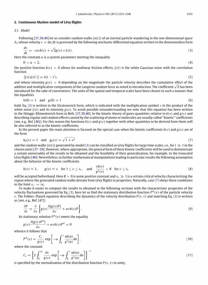

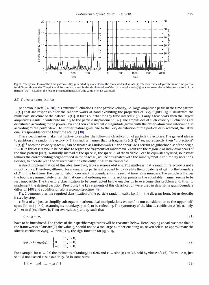


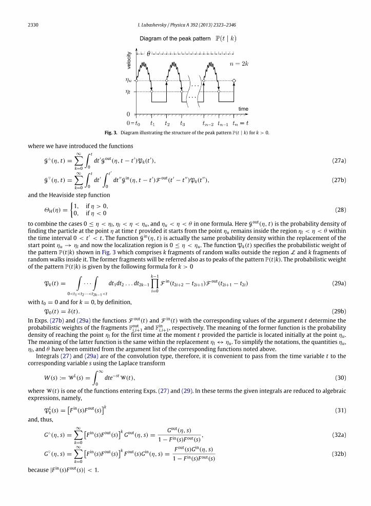


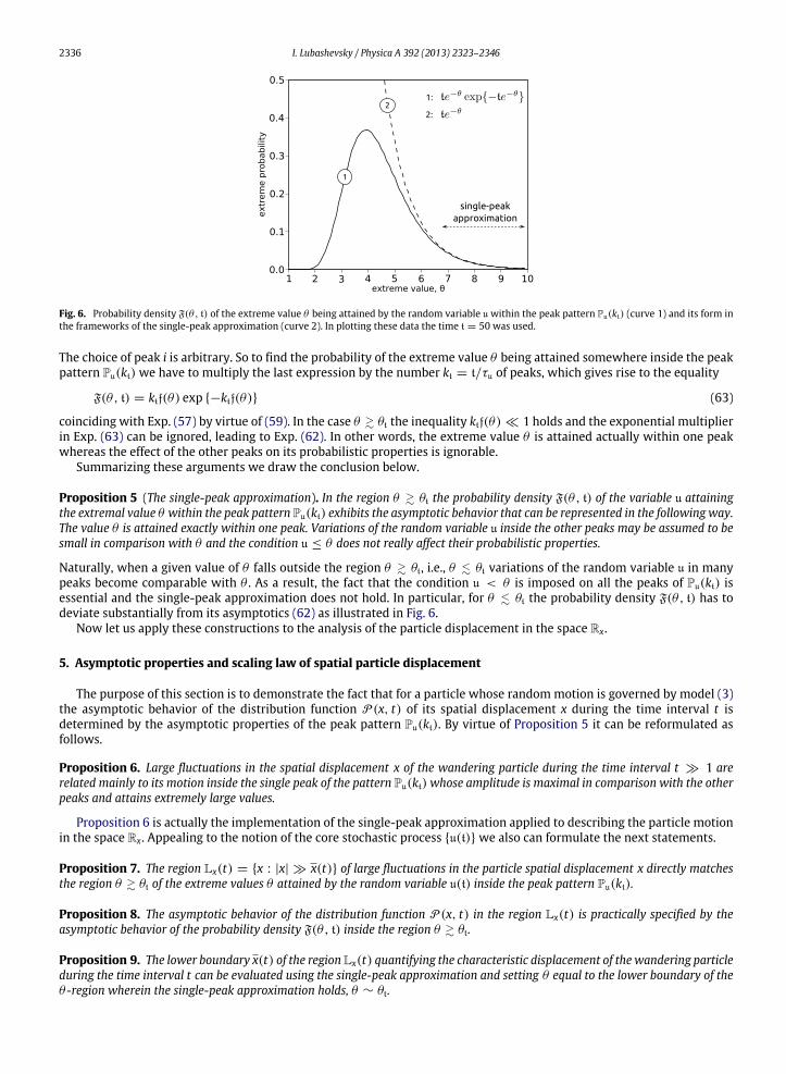


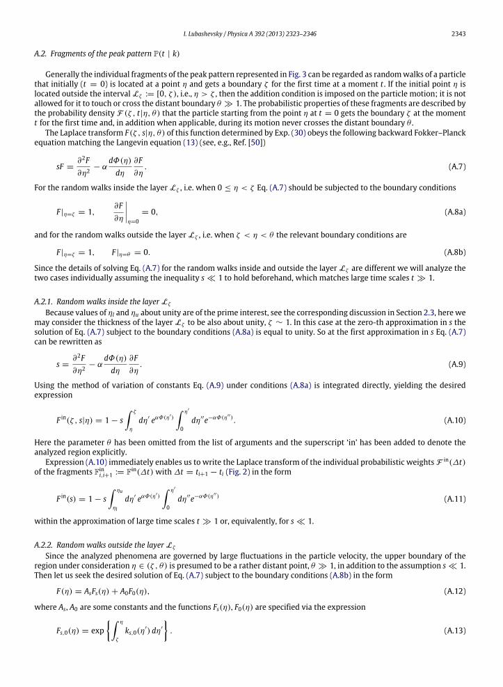


![[Roland Lévy, Jean-Michel Jonathan] L'Optique Non(BookZZ.org)](https://static.documents.pub/doc/80x56/55cf8efd550346703b97cf84/roland-levy-jean-michel-jonathan-loptique-nonbookzzorg.jpg)


