17
ERDAS IMAGINE 2015 RADAR Imagery Made Easy TIPS AND TRICKS USFWS WORKSHOP
ERDAS IMAGINE 2015
RADAR Imagery Made Easy
TIPS AND TRICKS
USFWS WORKSHOP


RadarAnalyst
SectionObjective Radar data is different from optical imagery both in its phenomenology and the types of information it records. While optical imagery gives you information about the chemical composition of features on the ground, radar data records information about the physical structure of the objects on the ground. This section is designed as an introduction to radar data and some of the basic tools for interpreting and analyzing radar images.
ToolsUsed
Radar Analyst Tab in IMAGINE which contains the tools for basic radar data analysis and exploitation.
Level Slice Visualize an image by slicing it into three levels based on their magnitude values in the image histogram.
Real‐time Enhancement Auto Enhance (Blue‐is‐New)

Exercise1:ViewingRadarData Objective:
Students will use a prepared radar image and learn how to identify different features in the imagery. Radar data is different from optical imagery in that it is echography and not photography. Light and dark pixels indicate not just the makeup of the landcover, but the physical structure and orientation of the features relative to the radar signal. In this Exercise, we will be looking at a Radarsat‐1 image of the border between Georgia and South Carolina. It is recording in the C‐band, with a wavelength of 5.6 cm. The pixels in this image are roughly 13 meters.
Task1.1:ViewingRadarDataandIdentifyingFeatures
1. Click File > Open > Raster Layer... c:\training\Fundamentals2\Radar select 2009_radar.img from the
data directory. Do not click OK yet.
2. On the Raster Options tab, select Orient Image to Map System.
This tells the software to read the calibration data that is included with the image and to project that image in the 2D View.
3. Click OK on the File selector dialog.
The radar image is displayed. Lake Hartwell is the large group of dark pixels in the middle of the image. In addition to the lakes, the bright reflections of the mountains in the north of the image are also apparent.
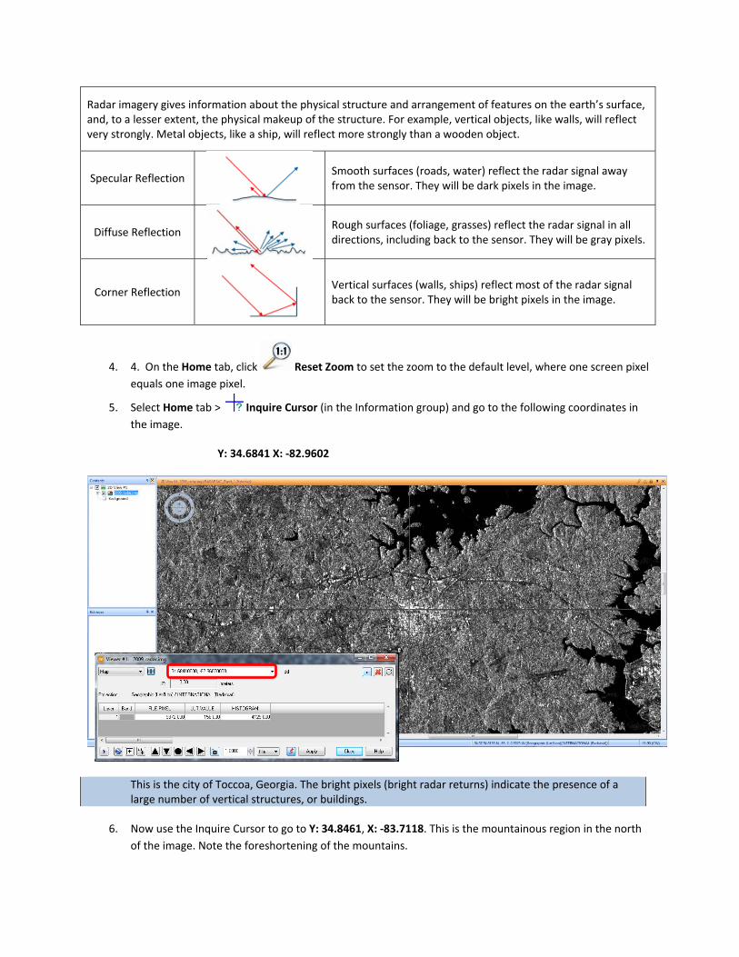
Radar imagery gives information about the physical structure and arrangement of features on the earth’s surface, and, to a lesser extent, the physical makeup of the structure. For example, vertical objects, like walls, will reflect very strongly. Metal objects, like a ship, will reflect more strongly than a wooden object.
Specular Reflection Smooth surfaces (roads, water) reflect the radar signal away from the sensor. They will be dark pixels in the image.
Diffuse Reflection Rough surfaces (foliage, grasses) reflect the radar signal in all directions, including back to the sensor. They will be gray pixels.
Corner Reflection Vertical surfaces (walls, ships) reflect most of the radar signal back to the sensor. They will be bright pixels in the image.
4. 4. On the Home tab, click Reset Zoom to set the zoom to the default level, where one screen pixel
equals one image pixel.
5. Select Home tab > Inquire Cursor (in the Information group) and go to the following coordinates in
the image.
Y: 34.6841 X: ‐82.9602
This is the city of Toccoa, Georgia. The bright pixels (bright radar returns) indicate the presence of a large number of vertical structures, or buildings.
6. Now use the Inquire Cursor to go to Y: 34.8461, X: ‐83.7118. This is the mountainous region in the north
of the image. Note the foreshortening of the mountains.

7. Use the Inquire Cursor to drive the view to Y: 34.4463, X: ‐83.1278.
The long, dark, linear feature stretching from southwest to northeast is the interstate highway. The relatively flat surface of the road reflects the radar signal away from the sensor, which the image displays as dark pixels.
8. Now use the Inquire Cursor to drive to the following coordinates and identify the features in the radar
image.
Coordinates Feature

Y: 34.6532 X: ‐82.8514
Y: 34.4933 X: ‐82.7137
Y: 34.3578 X: ‐82.8246
9. Close the Inquire Cursor.
Q: What is the look direction of the radar sensor? Hint: Zoom in on the mountains and look at the direction of the foreshortening?
Task1.2:TheRadarAnalystTabandLevelSlice
The Radar Analyst tab contains many of the functions used with radar data in IMAGINE.
1. On the Raster tab, select Radar Analyst.
2. On the Radar Analyst tab, select Look Direction.
A direction arrow is added to the View indicating the look direction of the radar system.
A Level Slice view allows you to try to isolate and visualize pixels based on their DN values. You will group the image into three groups, or slices: an Upper slice, a Center slice, and a Lower slice. You can
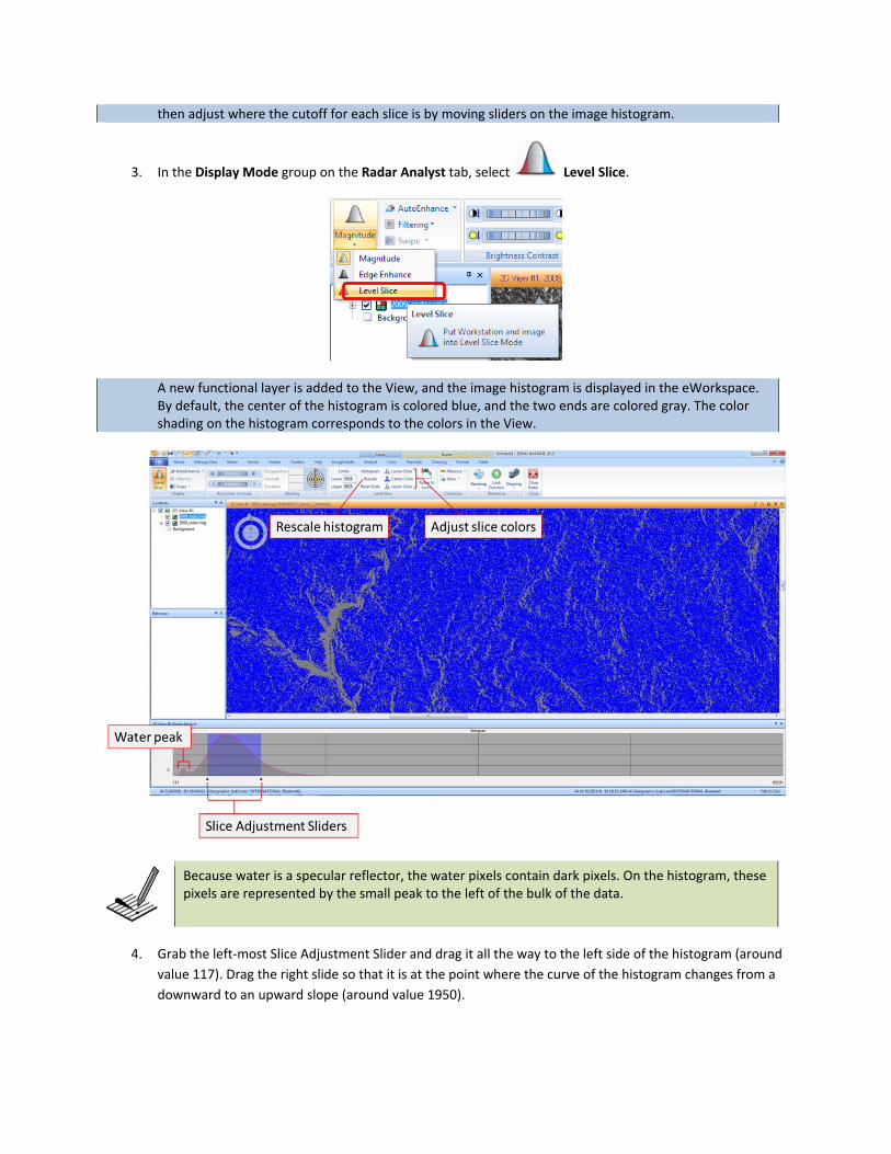
then adjust where the cutoff for each slice is by moving sliders on the image histogram.
3. In the Display Mode group on the Radar Analyst tab, select Level Slice.
A new functional layer is added to the View, and the image histogram is displayed in the eWorkspace. By default, the center of the histogram is colored blue, and the two ends are colored gray. The color shading on the histogram corresponds to the colors in the View.
Because water is a specular reflector, the water pixels contain dark pixels. On the histogram, these pixels are represented by the small peak to the left of the bulk of the data.
4. Grab the left‐most Slice Adjustment Slider and drag it all the way to the left side of the histogram (around
value 117). Drag the right slide so that it is at the point where the curve of the histogram changes from a
downward to an upward slope (around value 1950).

5. On the Radar Analyst toolbar select the Lower Color and change it to red. Do the same for the Upper
Color. Next, right click in the viewer and select Swipe.
This will allow you to compare the pseudocolor image you are manipulating via the histogram to the underlying original radar image. The goal is to optimize the land‐water separation.
6. Zoom in on one of the large water bodies in the image. Note the areas of water not included in the
selection. Adjust the sliders to include all of the water.
Note that there are erratic pixels that are seemingly misclassified e.g. bright “land” pixels in the water bodies. This is because we have been working with “raw” radar data that has not been despeckled. In the next exercise, we will talk more about speckle suppression, but right now, let’s just open a despeckled image.
7. Clear the View and open 2009_despeckle.img.
8. On the Raster tab, select > Radar Analyst.

Q: Can you display the Look Direction of the despeckled image?
9. In the Display Mode group on the Radar Analyst tab, select Level Slice.
Note that the two peaks of the bimodal histogram are more clearly resolved and separated. This is because the erratic pixel values resulting from speckle noise have been suppressed.
2009_Radar 2009_Despeckle
10. Adjust the sliders so that the blue area is between 307 and 3000.
11. On the Radar Analyst tab, in the Level Slice group, click the Rescale button. This will rescale the histogram
to only display the area between the two sliders.
12. Click on Upper Color in the toolbar to open the Color Chooser. Check use opacity and adjust the slider to
0. Do the same for the Lower Color.

13. Zoom in on the water body again.
14. Adjust the right slider back to the water/land breakpoint. Try to include as much water as possible.
15. When you are satisfied with your threshold setting. Click Raster to Vector on the Radar Analyst tab in the
Level Slice group.
16. Enter a name for the Output Shapefile, such as WaterTemp, and Intermediate Recorded Raster. Click OK
to calculate.
17. Close the Swipe Transition. On the Radar Analyst Workstation icon panel, return to Magnitude Mode.
18. Display the shapefile on top of the original radar image.
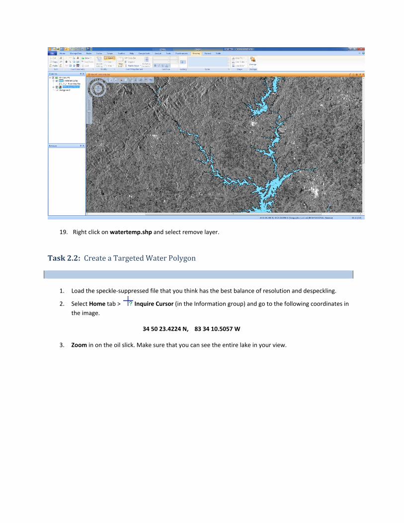
19. Right click on watertemp.shp and select remove layer.
Task2.2:CreateaTargetedWaterPolygon
1. Load the speckle‐suppressed file that you think has the best balance of resolution and despeckling.
2. Select Home tab > Inquire Cursor (in the Information group) and go to the following coordinates in
the image.
34 50 23.4224 N, 83 34 10.5057 W
3. Zoom in on the oil slick. Make sure that you can see the entire lake in your view.
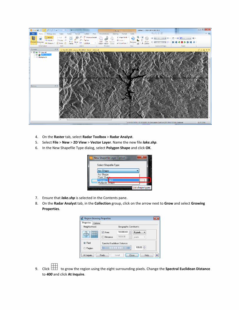
4. On the Raster tab, select Radar Toolbox > Radar Analyst.
5. Select File > New > 2D View > Vector Layer. Name the new file lake.shp.
6. In the New Shapefile Type dialog, select Polygon Shape and click OK.
7. Ensure that lake.shp is selected in the Contents pane.
8. On the Radar Analyst tab, in the Collection group, click on the arrow next to Grow and select Growing
Properties.
9. Click to grow the region using the eight surrounding pixels. Change the Spectral Euclidean Distance
to 400 and click At Inquire.

A small polygon is created. At this Spectral Euclidean distance it is much too small to encompass the majority of the slick.
10. Use the thumbwheel to increase the distance to 800. When you let go of the wheel, the polygon updates
to show the region grown by the new settings.
11. Continue adjusting the Distance until you have grown the polygon to include all connected water.
12. Save the shapefile.
13. Continue digitizing the individual lakes. Save the file after each polygon is collected.
Exercise3:Blue‐is‐New Objective:
In this exercise we will use the real‐time Change Detection Tool in the Radar Analyst Workstation.
Task3:Identifyglacialmovementusingradarimagery
Blue‐is‐New
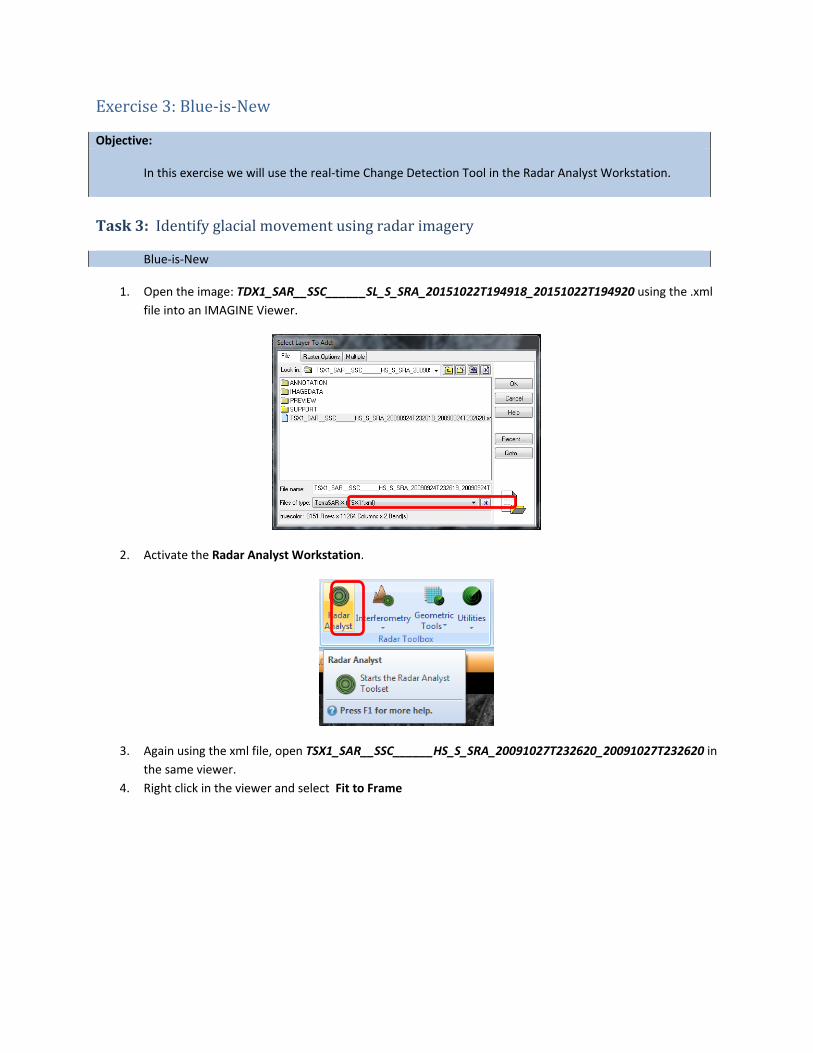
1. Open the image: TDX1_SAR__SSC______SL_S_SRA_20151022T194918_20151022T194920 using the .xml
file into an IMAGINE Viewer.
2. Activate the Radar Analyst Workstation.
3. Again using the xml file, open TSX1_SAR__SSC______HS_S_SRA_20091027T232620_20091027T232620 in
the same viewer.
4. Right click in the viewer and select Fit to Frame
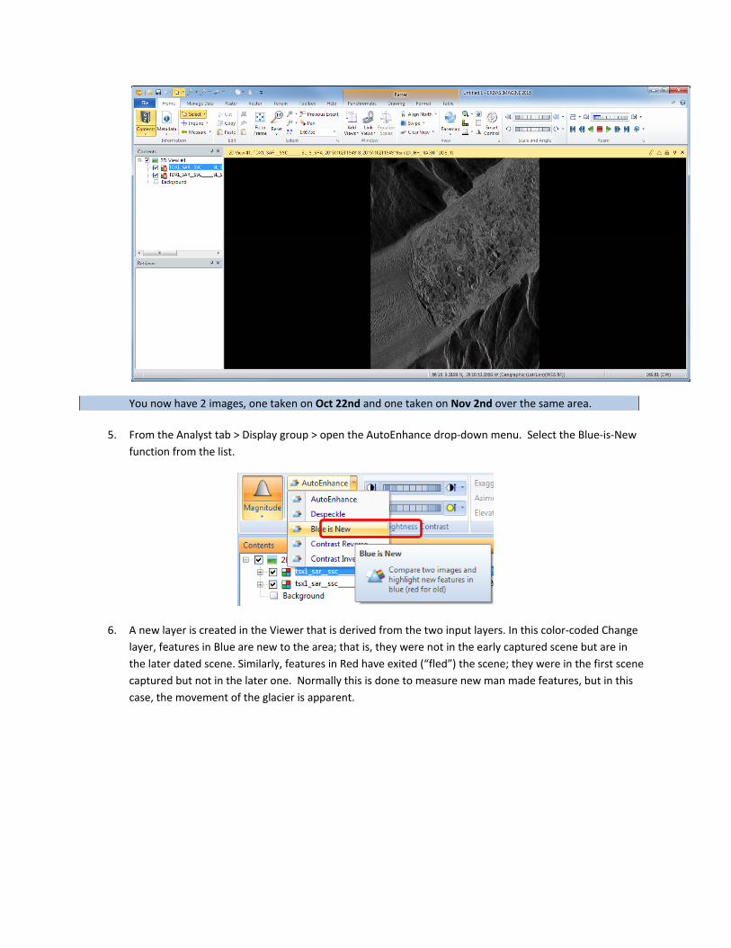
You now have 2 images, one taken on Oct 22nd and one taken on Nov 2nd over the same area.
5. From the Analyst tab > Display group > open the AutoEnhance drop‐down menu. Select the Blue‐is‐New
function from the list.
6. A new layer is created in the Viewer that is derived from the two input layers. In this color‐coded Change
layer, features in Blue are new to the area; that is, they were not in the early captured scene but are in
the later dated scene. Similarly, features in Red have exited (“fled”) the scene; they were in the first scene
captured but not in the later one. Normally this is done to measure new man made features, but in this
case, the movement of the glacier is apparent.

7. Clear all views.


