ERDC/CHL CHETN-VII-19 June 2018 Approved for public release; distribution is unlimited. Modeling Flap Gate Culverts in Adaptive Hydraulics (AdH) by C. Jared McKnight, Gaurav Savant, Jennifer N. McAlpin, and Tate O. McAlpin PURPOSE: This Coastal and Hydraulics Engineering Technical Note (CHETN) describes the methodology and implementation of flap gate culverts in the 2-D Shallow Water (SW2D) version of Adaptive Hydraulics (AdH). See Figure 2 for an example of this type of structure. This technical note will outline how to calculate the culvert coefficient (K) for flap gate culverts for use in AdH and present a test case detailing the implementation of the structure into AdH input files. A synopsis of the test case results is also presented. Figure 1. Example of flap gate culverts. (This photo was taken from Google Images). BACKGROUND: Diversion-structure culverts are represented in AdH as an internal boundary condition that specifies the head difference/discharge relationship for the structure. The basic equation for culvert flow is Equation 1 from Brater et al. (1996): 2 Q Ca gh = (1) where: culvert discharge coefficient of discharge opening area gravity head difference across the structure Q C a g h = = = = =
Transcript
ERDC/CHL CHETN-VII-19 June 2018
Approved for public release; distribution is unlimited.
Modeling Flap Gate Culverts in Adaptive
Hydraulics (AdH)
by C. Jared McKnight, Gaurav Savant, Jennifer N. McAlpin, and Tate O. McAlpin
PURPOSE: This Coastal and Hydraulics Engineering Technical Note (CHETN) describes the methodology and implementation of flap gate culverts in the 2-D Shallow Water (SW2D) version of Adaptive Hydraulics (AdH). See Figure 2 for an example of this type of structure. This technical note will outline how to calculate the culvert coefficient (K) for flap gate culverts for use in AdH and present a test case detailing the implementation of the structure into AdH input files. A synopsis of the test case results is also presented.
Figure 1. Example of flap gate culverts. (This photo was taken from Google
Images).
BACKGROUND: Diversion-structure culverts are represented in AdH as an internal boundary condition that specifies the head difference/discharge relationship for the structure. The basic equation for culvert flow is Equation 1 from Brater et al. (1996):
2Q Ca gh= (1)
where:culvert dischargecoefficient of dischargeopening areagravityhead difference across the structure
QCagh
=====
ERDC/CHL CHETN-VII-19 June 2018
2
There are two scenarios under which a flap gate culvert could be incorporated into an AdH model. First, there is a need to design a culvert, and AdH is being used to test the design. Second, an existing flap gate culvert is already in place within an AdH model domain. For the first scenario, the head-discharge relationship shown in Equation 2 can be used directly to calculate the culvert coefficient (K) for a known flow rate and desired head difference:
The friction factors for the culverts and channel are calculated using a Manning’s n roughness value for the different materials found in Brater et al. (1996). A Manning’s n of 0.016, which is a standard design value for concrete channels, can be used for a concrete culvert. A Manning’s n of 0.025, which corresponds to a natural, straight, full stage channel in very good shape, can be used for the channel. The Manning’s n value will vary depending on the system. Using Equation 4, which illustrates the relationship between the Darcy friction factor and Manning’s n from Limerinos (1970), friction factors can be calculated for any culvert arrangement:
Implementation within AdH consists of using reference strings upstream/downstream of the actual structure to determine the head differential across the gate used to compute the discharge (see Figure 2). This implementation was chosen because Equation 1 is derived from a momentum balance at locations where the local effect of the structure does not distort the flow. To account for the losses occurring in these approach and release channels, which is the distance between the reference strings and the structure, additional losses must be incorporated beyond the culvert frictional losses.
Equation 5 includes the channel, culvert, entrance, exit, and flap gate frictional losses:
( ) ( )2 2
2
2
2 2
4 2 4 2
4 2
culvert f culvert culvert channel gate entrance exit
culvert culvertculvert culvert culvert
culvert culvert culvert
channel channchannel channel channel
channel
Q Ca g h h Ca g h h h h h h
L V L Qh f fr g r ga
L V Lh f fr g
= − = − − − − −
= =
= =2
2
2 2
2
2 2
2
2 2
2
4 2
2 2
2 2
2 2
el
channel channel
gate gate gateculvert
entrance entrance entranceculvert
exit exit exitculvert
Qr ga
V Qh K Kg a g
V Qh K Kg a g
V Qh K Kg a g
= =
= =
= =
(5)
Brater et al. (1996) provide equations for the discharge coefficient for concrete box culverts that include a rounded-lip entrance (Equation 6). Equations for other arrangements are also included in this reference.
1/2
1.250.00331.05 LC
R
− = +
(6)
where:culvert lengthculvert hydraulic radius
LR==
ERDC/CHL CHETN-VII-19 June 2018
4
Figure 2. Locations of node strings and edge strings for flap gate test case.
Equation 6 was derived from experimental results with culvert lengths of 7 to 11 meters (m), so longer culverts require a different method to calculate the added frictional head loss.
This method is derived by rearranging and solving for the culvert discharge Q:
mod2 2 22
2
2
14 4
culvert elculvert channel culvert
culvert channel mculvert channel channel
ghQ Ca K hL C L C af f K C
r r a
= =+ + +
(7)
where: minor losses
0.1 for high energy flow according to Replogle and Wahlin (2003) 1 from Brater et al. (1996)
0.1 from Brater et al. (1996)
m gate exit entrance
gate
exit
entrance
K K K KKK
K
= = + +
=
==
According to Replogle and Wahlin (2003), the minor gate loss coefficient can vary from 0.1, for large velocity head flows, to 1, for very low velocity head flows with fully submerged flow. If the velocity head within the culverts will be large, the smallest value of Kgate can be assumed. Kexit and Kentrance are standard loss coefficients for exits and entrances taken from Brater et al. (1996).
Consider a scenario where a flap gate culvert is being designed and tested using AdH with desired parameters and a loss coefficient K is sought. The flow rate is 200.96 cubic meters per second (cms), the recommended head differential is 0.73 m, and the culvert discharge coefficient
ERDC/CHL CHETN-VII-19 June 2018
5
is 235.2 m5/2/s. If Scenario 2 is assumed, then the system parameters must be used in Equation 7 to calculate K.
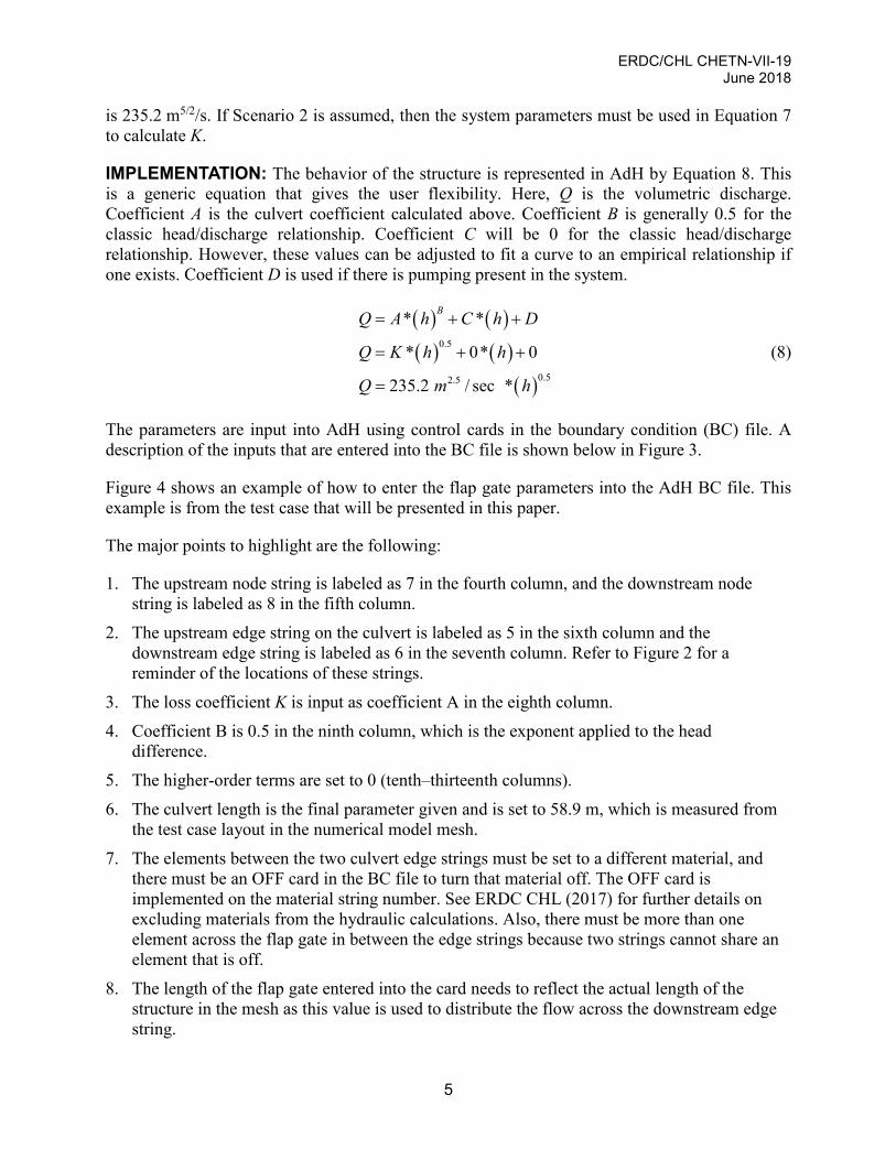
IMPLEMENTATION: The behavior of the structure is represented in AdH by Equation 8. This is a generic equation that gives the user flexibility. Here, Q is the volumetric discharge. Coefficient A is the culvert coefficient calculated above. Coefficient B is generally 0.5 for the classic head/discharge relationship. Coefficient C will be 0 for the classic head/discharge relationship. However, these values can be adjusted to fit a curve to an empirical relationship if one exists. Coefficient D is used if there is pumping present in the system.
( ) ( )( ) ( )
( )
0.5
0.52.5
* *
* 0* 0
235.2 / sec *
BQ A h C h D
Q K h h
Q m h
= + +
= + +
=
(8)
The parameters are input into AdH using control cards in the boundary condition (BC) file. A description of the inputs that are entered into the BC file is shown below in Figure 3.
Figure 4 shows an example of how to enter the flap gate parameters into the AdH BC file. This example is from the test case that will be presented in this paper.
The major points to highlight are the following:
1. The upstream node string is labeled as 7 in the fourth column, and the downstream node string is labeled as 8 in the fifth column.
2. The upstream edge string on the culvert is labeled as 5 in the sixth column and the downstream edge string is labeled as 6 in the seventh column. Refer to Figure 2 for a reminder of the locations of these strings.
3. The loss coefficient K is input as coefficient A in the eighth column. 4. Coefficient B is 0.5 in the ninth column, which is the exponent applied to the head
difference. 5. The higher-order terms are set to 0 (tenth–thirteenth columns). 6. The culvert length is the final parameter given and is set to 58.9 m, which is measured from
the test case layout in the numerical model mesh. 7. The elements between the two culvert edge strings must be set to a different material, and
there must be an OFF card in the BC file to turn that material off. The OFF card is implemented on the material string number. See ERDC CHL (2017) for further details on excluding materials from the hydraulic calculations. Also, there must be more than one element across the flap gate in between the edge strings because two strings cannot share an element that is off.
8. The length of the flap gate entered into the card needs to reflect the actual length of the structure in the mesh as this value is used to distribute the flow across the downstream edge string.
ERDC/CHL CHETN-VII-19 June 2018
6
Figure 3. Description of flap gate card (ERDC CHL 2017).
Figure 4. Example of flap gate card from test case BC file.
TEST CASE FORCING: The test case was forced with the following arrangement:
1. Inflow Boundary a. The volumetric flow was linearly increased from 0 cms to 200.96 cms over the first 6
hours (hr). b. The flow rate was then held constant over the next 30 hr. c. The flow rate was then linearly decreased to 0 cms from 36 to 42 hr. d. The flow rate was held at 0 cms for the final 6 hr of the simulation.
2. Tidal Boundary a. The water surface elevation was held at a constant tailwater equal to the initial depth for
the first 10 hr. b. The tidal range then varied over a 4 m range for the last 38 hr.
ERDC/CHL CHETN-VII-19 June 2018
7
Figure 5. Location of boundaries for test case.
COMMON PROBLEMS: When running AdH with flap gate culverts, two main issues may arise. First, numerical instabilities or ringing associated with the flap gate structure can be a problem. Such behavior is most troublesome during ramping and also with tidal signals. An example of ringing, as indicated by the oscillations in the solution (easily seen in the green and red lines) is shown in Figure 6. These instabilities dominate during ramping and are also prevalent during the tidal simulation. The second major issue is that the flap gate solver is outside the finite element scheme, so mass is not fully conserved. For simple examples, like this test case, the lost mass is negligible and is approximately three orders of magnitude smaller for this test case. For more complicated systems, sensitivity analysis has shown the solution converges to within 2% of the appropriate flow rate.
Another example of ringing is shown in Figure 7. The model time-step size was reduced from 120 seconds to 1 second. With the smaller time-step, the instabilities are now only prevalent during the ramping up or down. The 1 second time-step causes increased ringing as high frequency waves are created by the structure turning on/off and resolved within the AdH model. Larger time-steps diffuse these waves reducing the oscillations but sometimes causing the creation of other oscillations.
ERDC/CHL CHETN-VII-19 June 2018
8
Figure 6. Example of ringing from the test case with a 120 s time-step.
ERDC/CHL CHETN-VII-19 June 2018
9
Figure 7. Example of ringing from the test case with a 1 s time-step.
CHOOSING A TIME-STEP: Choosing an appropriate time-step can reduce the oscillations. The time-step can be estimated by using the general relationship between wave speed, time, and distance. See Equation 9.
( )t gh U d+ ≤ (9)
where: time-step
shallow water wave celerity free stream velocity
distance from nodestring to structure
t
ghU
d
=
=
==
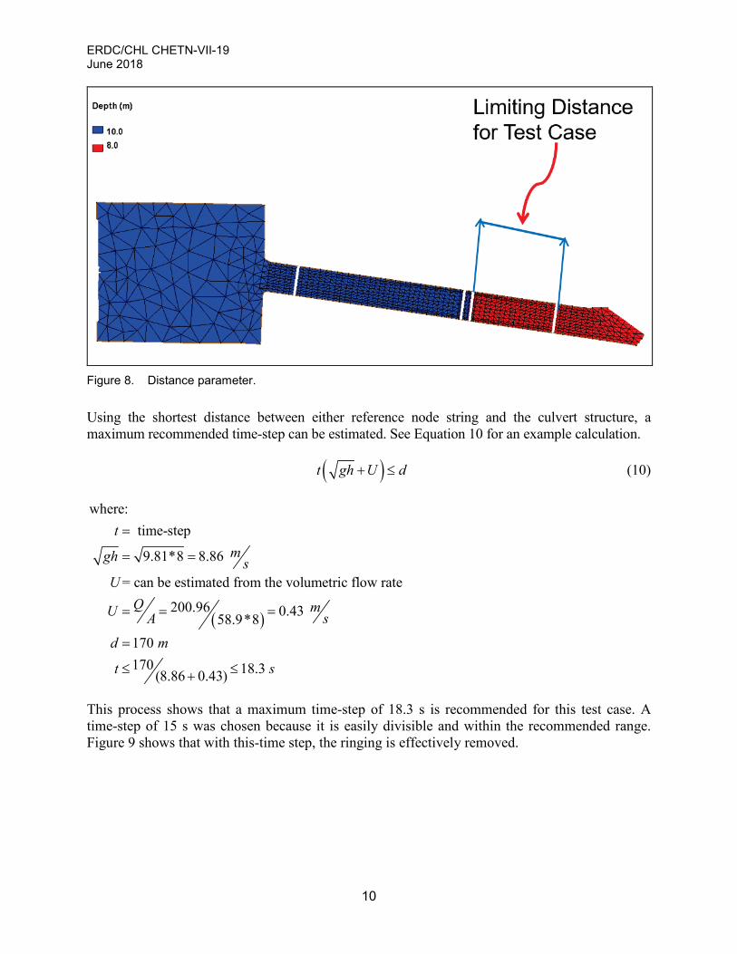
See Figure 8 for an illustration of the limiting distance for this test case.
ERDC/CHL CHETN-VII-19 June 2018
10
Figure 8. Distance parameter.
Using the shortest distance between either reference node string and the culvert structure, a maximum recommended time-step can be estimated. See Equation 10 for an example calculation.
( )t gh U d+ ≤ (10)
( )
where: time-step
9.81*8 8.86
= can be estimated from the volumetric flow rate
200.96 0.43 58.9*8170 170 18.3 (8.86 0.43)
tmgh s
UQ mU A s
d m
t s
=
= =
= = =
=
≤ ≤+
This process shows that a maximum time-step of 18.3 s is recommended for this test case. A time-step of 15 s was chosen because it is easily divisible and within the recommended range. Figure 9 shows that with this-time step, the ringing is effectively removed.
ERDC/CHL CHETN-VII-19 June 2018
11
Figure 9. Discharge using a 15 s time-step.
Looking back to Figure 7, the 1 s time-step theoretically should have been stable. However, at very small time-steps, high-frequency oscillations can occur during ramping. AdH is capable of resolving these oscillations using small time-steps causing increased ringing. An example of the high-frequency oscillations, represented by the water surface elevation (WSE) at the upstream reference node string, is shown in Figure 10. At larger time-steps, these oscillations are not resolved.
Figure 10. High-frequency oscillations.
ERDC/CHL CHETN-VII-19 June 2018
12
If a smaller time-step is necessary for a simulation due to other limiting factors beyond the culvert structure, there are approaches to remove this high-frequency signal. Expanding the area of the reference node strings will increase stability. The area the node strings encompass must be realistic for the structure-head difference calculation. The node strings must not be placed on the edge of the culvert structure or on an open boundary. The length across the node string must be larger than the high-frequency wavelength. See Figure 11 for an illustration of how to implement the strings.
Figure 11. Extended node strings to remove high-frequency oscillation.
Figure 12 shows that by implementing the node strings as shown, the ringing is significantly reduced.
Figure 12. Comparison of flux output with a single node string and the extended node string.
Using this approach will allow for the use of a smaller time-step if other issues within the system make such time-steps necessary.
TEST CASE RESULTS/PROOF OF CONCEPT: The test case was run with a 15 s time-step with automatic mesh adaption included. Figure 13 illustrates the behavior of the culvert for the
ERDC/CHL CHETN-VII-19 June 2018
13
test case. As the inflow increases, the upstream water elevation overtakes the downstream water elevation causing the culvert to turn on. That flow is then held steady for 4 hr, and the head differential is constant. With the addition of tides, the upstream water surface elevation corrects and stays ahead of the downstream, so the tidal effect is seen on both sides of the structure. The flow is then decreased until the upstream and downstream elevations are equal, which causes the culvert to turn off. Finally, the upstream elevation returns to its initial value.
Figure 13. Upstream and downstream water surface elevation (WSE) for test case.
Using the discharge/head relationship shown in Equation 2 and the model elevation output at the reference strings, theoretical volumetric fluxes were compared to volumetric fluxes from the model solution during the steady state (6–10 hr) and the tidal (10–36 hr) ranges of the simulation.
The values in Table 1 indicate that the model is accurate at estimating the culvert flow. In general, AdH-SW2D slightly underpredicts the flux compared to the theoretical values. The steady state comparison was calculated at the end of the steady state portion (6–10 hr), and the tidal comparison is an average over the tidal time range before the ramp down (10–36 hr).
ERDC/CHL CHETN-VII-19 June 2018
14
Table 1. Comparison of theoretical volumetric flow rates (m3/s) to model output. Model Range Steady State Tidal Theoretical 200.96 200.605 Model 200.61 200.07 % Diff 0.17 0.27
SUMMARY OF FINDINGS: AdH-SW2D is accurate at modeling flap-gate culvert flow. Time-step choice and the arrangement of the reference node strings are the most important steps to implementing this structure in AdH-SW2D. By appropriately estimating a time-step and setting up the reference node strings in a reasonable and realistic manner, instabilities will be dramatically reduced, and the model should accurately predict the flow through the system.
ADDITIONAL INFORMATION: For additional information, contact Jared McKnight, Research General Engineer, Coastal and Hydraulics Laboratory, U.S. Army Engineer Research and Development Center, 3909 Halls Ferry Road, Vicksburg, MS 39180-6199; phone: 601-634-2844; email: [email protected]. This effort was funded through the 219 Office of Research and Technology Transfer (ORTT) Initiatives Technology Transition Advancement Program.
McKnight, C. J., G. Savant, J. N. McAlpin, and T. O. McAlpin. 2018. Modeling Flap Gate Culverts in Adaptive Hydraulics (AdH). ERDC/CHL CHETN-VII-19. Vicksburg, MS. U.S. Army Engineer Research and Development Center. http://dx.doi.org/10.21079/11681/27414
REFERENCES Brater, E. F., H. W. King, J. E. Lindell, and C. Y. Wei. 1996. Handbook of Hydraulics. New York: McGraw-Hill.
Limerinos, J. T. 1970. Determination of the Manning Coefficient from Measured Bed Roughness in Natural Channels. Geological Survey Water-Supply Paper 1898-B. Washington, DC: United States Government Printing Office.
Replogle, J. A., and B. T. Wahlin. 2003. “Head Loss Characteristics of Flap Gates at the Ends of Drain Pipes.” American Society of Agricultural Engineers 46(4): 1077–1084.
U.S. Army Engineer Research and Development Center (ERDC), Coastal and Hydraulics Laboratory (CHL). 2017. Adaptive Hydraulics 2D Shallow Water (AdH-SW2D) User Manual (Version 4.6). Vicksburg, MS: U.S. Army Engineer Research and Development Center. https://chl.erdc.dren.mil/adh/documentation/AdH_Manual_ Hydrodynamic-Version4.6.pdf.
NOTE: The contents of this technical note are not to be used for advertising, publication, or promotional purposes. Citation of trade names does not constitute an official
endorsement or approval of the use of such products.