ERDC/EL CR-14-3 Environmental Quality and Installations (EQI) Research Program Evaluation of Time-Varying Hydrology within the Training Range Environmental Evaluation and Characterization System (TREECS™) Environmental Laboratory Mark S. Dortch August 2014 Approved for public release; distribution is unlimited.
Transcript
ERD
C/EL
CR-
14-3
Environmental Quality and Installations (EQI) Research Program
Evaluation of Time-Varying Hydrology within the Training Range Environmental Evaluation and Characterization System (TREECS™)
Envi
ronm
enta
l Lab
orat
ory
Mark S. Dortch August 2014
Approved for public release; distribution is unlimited.
The US Army Engineer Research and Development Center (ERDC) solves the nation’s toughest engineering and environmental challenges. ERDC develops innovative solutions in civil and military engineering, geospatial sciences, water resources, and environmental sciences for the Army, the Department of Defense, civilian agencies, and our nation’s public good. Find out more at www.erdc.usace.army.mil.
To search for other technical reports published by ERDC, visit the ERDC online library at http://acwc.sdp.sirsi.net/client/default.
Evaluation of Time-Varying Hydrology within the Training Range Environmental Evaluation and Characterization System (TREECS™)
Mark S. Dortch Contractor for Los Alamos Technical Associates, Inc. 999 Central Avenue, #300 Los Alamos, NM 87544
Final report Approved for public release; distribution is unlimited.
Prepared for U.S. Army Corps of Engineers Washington, DC 20314-1000
ERDC/EL CR-14-3 ii
Abstract
The Training Range Environmental Evaluation and Characterization System (TREECS™) uses average annual hydrologic conditions as inputs for multi-media fate and transport models. This simplification reduces model complexity and data input requirements while providing the capability to conduct long-term predictions of the fate of munitions constituents (MC) as well as other contaminants. TREECS™ was recently modified to allow the option of using time-varying (daily) hydrology for forcing input conditions. This report summarizes the results of testing this new feature. MC fate predictions with daily hydrology are compared with those using average annual hydrology. Results show that the use of average annual hydrology produces more conservative results (i.e., higher media concentrations) than using daily hydrology. A validation application for lead downstream of small arms firing ranges is also presented in this report. The daily hydrology feature will be most useful for applications involving short periods (year or less) to evaluate the effects of variable precipitation and flow on MC concentrations in streams.
DISCLAIMER: The contents of this report are not to be used for advertising, publication, or promotional purposes. Citation of trade names does not constitute an official endorsement or approval of the use of such commercial products. All product names and trademarks cited are the property of their respective owners. The findings of this report are not to be construed as an official Department of the Army position unless so designated by other authorized documents. DESTROY THIS REPORT WHEN NO LONGER NEEDED. DO NOT RETURN IT TO THE ORIGINATOR.
ERDC/EL CR-14-3 iii
Contents Abstract .......................................................................................................................................................... ii
Figures and Tables ......................................................................................................................................... v
Unit Conversion Factors ........................................................................................................................... viii
Acronyms, Abbreviations, and Symbols .................................................................................................. ix Mathematical Symbols ............................................................................................................. x
2 Test Conditions ...................................................................................................................................... 4 Application site ......................................................................................................................... 4 Tier and media selections ........................................................................................................ 5 Site Conditions screen inputs .................................................................................................. 5 Precipitation and air temperature inputs ................................................................................ 6 Hydrology and erosion .............................................................................................................. 8 Tier 2 soil model inputs............................................................................................................ 9 CMS inputs ............................................................................................................................. 11 Vadose zone and aquifer model inputs................................................................................. 13
3 Comparison of Test Results .............................................................................................................. 15 Fate process fluxes in AOI soil ............................................................................................... 15
Appendix A: Summary of Methods for Computing Time-Varying Water Balance and Erosion for Surface Soil ..................................................................................................................... 47
Report Documentation Page
ERDC/EL CR-14-3 v
Figures and Tables
Figures
Figure 1. Site map for Ranges 20–22 at Fort Leonard Wood, Missouri. ............................................... 5 Figure 2. Comparison of lead dissolution fluxes versus time within AOI soil for TV (daily hydrology) and AA (average annual hydrology) test conditions. ............................................................. 16 Figure 3. Comparison of RDX dissolution fluxes versus time within AOI soil for TV (daily hydrology) and AA (average annual hydrology) test conditions. ............................................................. 16 Figure 4. Comparison of lead erosion fluxes versus time for AOI soil for TV (daily hydrology) and AA (average annual hydrology) test conditions. ................................................................................ 18 Figure 5. Comparison of RDX erosion fluxes versus time for AOI soil for TV (daily hydrology) and AA (average annual hydrology) test conditions. ................................................................................ 19 Figure 6. Comparison of lead leaching fluxes versus time within AOI soil for TV (daily hydrology) and AA (average annual hydrology) test conditions. ............................................................. 20 Figure 7. Comparison of RDX leaching fluxes versus time within AOI soil for TV (daily hydrology) and AA (average annual hydrology) test conditions. ............................................................. 20 Figure 8. Comparison of lead runoff fluxes versus time from AOI soil for TV (daily hydrology) and AA (average annual hydrology) test conditions. ............................................................. 22 Figure 9. Comparison of RDX runoff fluxes versus time from AOI soil for TV (daily hydrology) and AA (average annual hydrology) test conditions. ............................................................. 23 Figure 10. Comparison of RDX volatilization fluxes versus time within AOI soil for TV (daily hydrology) and AA (average annual hydrology) test conditions. ............................................................. 24 Figure 11. Comparison of lead flux to surface water versus time for TV (daily hydrology) and AA (average annual hydrology) test conditions. ................................................................................ 25 Figure 12. Comparison of RDX flux to surface water versus time for TV (daily hydrology) and AA (average annual hydrology) test conditions. ................................................................................ 25 Figure 13. Comparison of dissolved RDX flux from vadose zone to aquifer versus time for TV (daily hydrology) and AA (average annual hydrology) test conditions. ............................................. 27 Figure 14. Comparison of lead total concentration in AOI soil versus time for TV (daily hydrology) and AA (average annual hydrology) test conditions. ............................................................. 28 Figure 15. Comparison of RDX total concentration in AOI soil versus time for TV (daily hydrology) and AA (average annual hydrology) test conditions. ............................................................. 29 Figure 16. Comparison of RDX aquifer concentration at receptor well versus time for TV (daily hydrology) and AA (average annual hydrology) test conditions. ................................................... 29 Figure 17. Comparison of stream sediment total concentration of lead at receptor location versus time for TV (daily hydrology) and AA (average annual hydrology) test conditions. .................. 31 Figure 18. Comparison of stream sediment total concentration of RDX at receptor location versus time for TV (daily hydrology) and AA (average annual hydrology) test conditions. ..................................................................................................................................................... 31 Figure 19. Comparison of stream sediment total concentration of RDX at receptor location versus time for TV (daily hydrology) and AA (average annual hydrology) test conditions (using log concentration). ........................................................................................................ 32
ERDC/EL CR-14-3 vi
Figure 20. Comparison of stream water column total concentration of lead at receptor location versus time for TV (daily hydrology) and AA (average annual hydrology) test conditions. ..................................................................................................................................................... 33 Figure 21. Comparison of stream water column total concentration of RDX at receptor location versus time for TV (daily hydrology) and AA (average annual hydrology) test conditions. ..................................................................................................................................................... 33 Figure 22. Lead total concentration in water column versus time at the downstream terminus of the modeled Falls Hollow reach for the 2012 validation application. ............................. 37 Figure 23. Lead total concentration in benthic sediment versus time at the downstream terminus of the modeled Falls Hollow reach for the 2012 validation application. .......................... 38 Figure A1. SCS 24-hr rainfall distribution (from Ponce (1989)). ............................................................ 51 Figure A2. SCS 24-hr rainfall distribution map (from Ponce (1989)). ................................................... 52
Tables
Table 1. RDX properties selected from the Army Range Constituent Database. .................................. 6 Table 2. Average annual outputs computed by HGCT applied for time-varying hydrology using hourly precipitation. ............................................................................................................................. 9 Table 3. Tier 2 soil model inputs for AA test case. ..................................................................................... 9 Table 4. CMS inputs for AA test case. ........................................................................................................ 11 Table 5. MEPAS vadose zone model inputs. ............................................................................................ 13 Table 6. MEPAS Aquifer model inputs. ...................................................................................................... 14 Table 7. Summary of test results. ............................................................................................................... 34 Table A1. Coefficients for runoff peak unit discharge equation (from Haan et al. (1994)). .............. 52 Table A2. Surface storage correction factor. ............................................................................................ 53
ERDC/EL CR-14-3 vii
Preface
This study was funded by the U.S. Army’s Environmental Quality and Installations (EQI) Research Program. The work reported herein was conducted by Dr. Mark Dortch of MSD Engineering Consulting under contract to Los Alamos Technical Associates, which was under contract to the U.S. Army Engineer Research and Development Center (ERDC). Dr. Dortch prepared this report.
The study was conducted under the general direction of Dr. Beth Fleming, Director, Environmental Laboratory (EL); Dr. Jack Davis, Deputy Director, EL; Warren Lorentz, Chief, Environmental Processes and Effects Division; and Dr. Dorothy Tillman, Chief, Water Quality and Contaminant Modeling Branch (WQCMB). Dr. Elizabeth Ferguson was Technical Director of military environmental research, and John Ballard was Program Manager for the EQI Range Research Program.
Acknowledgements are made to Mark R. Noel and Jeffrey A. Gerald of WQCMB who performed the computer program coding changes required for this project.
Dr. Jeffery P. Holland was Director of ERDC. COL Jeffrey Eckstein was Commander. This report is approved for unlimited distribution.
ERDC/EL CR-14-3 viii
Unit Conversion Factors
Multiply By To Obtain
acres (p. 73) 4,046.873 square meters
cubic feet per second 0.0283 cubic meters per second
feet 0.3048 meters
inches 25.4 millimeters
inches 0.0254 meters
liters 1,000 cubic meters
metric tons 1,000 kilograms
pounds (mass) (p. 73) 0.4535924 kilograms
square miles 2.59 square kilometers
U.S. tons 0.907 metric tons
ERDC/EL CR-14-3 ix
Acronyms, Abbreviations, and Symbols
Acronyms and Abbreviations
AA test case using average annual hydrology AOI area of interest, such as small arms range impact areas BMP(s) Best Management Practice(s) CMS Contaminant Model for Streams CN SCS curve number DoD Department of Defense DODIC Department of Defense Identification Code for munitions
items EL Environmental Laboratory ERDC Engineer Research and Development Center EQI U.S. Army’s Environmental Quality and Installations
Research Program GB giga-bytes or one billion bytes GHz giga-Hertz or one billion cycles per second GIS geographical information system HE high explosives HGCT Hydro-Geo-Chemical Toolkit within TREECS™ NCDC National Climatic Data Center of NOAA NOAA National Oceanographic and Atmospheric Administration MC munitions constituents, such as metals and high explosives MEPAS Multimedia Environmental Pollutant Assessment System
groundwater model (vadose and aquifer) MT metric tons MUSLE Modified Universal Soil Loss Equation used to compute soil
erosion rate for time-varying hydrology NSN National Stock Number for munitions items ppb parts per billion SAFRs small arms firing ranges SCS Soil Conservation Service TREECS™ Training Range Environmental and Evaluation System TSS total suspended solids concentration TV test case using time-varying (daily) hydrology UI user interface of a model USGS U.S. Geological Survey USLE Universal Soil Loss Equation used to compute soil erosion
rate for average annual hydrology
ERDC/EL CR-14-3 x
Mathematical Symbols
A catchment or AOI surface area, m2 As sediment yield from overland soil erosion for a rainfall event,
MT C crop management factor in the USLE and MUSLE C0, C1, C2 regression coefficients in the equation to relate qu to tc that
are based on rainfall type and Ia/P, unit-less E soil erosion rate, m/year or m/day ET average annual evapotranspiration rate, m/yr ETt daily evapotranspiration rate, m/day F surface storage correction factor for runoff in the TR-55
method, unit-less H surface soil layer thickness, m Hro runoff depth for a rainfall event in the TR-55 methods,
inches I average annual infiltration rate for day t, m/yr Ia initial abstraction in the SCS curve number runoff method,
inches or m It daily infiltration rate for day t, m/day K soil erodibility factor in the USLE and MUSLE L length of the catchment principle water course from basin
outlet to divide (i.e., upstream extent of AOI draining towards outlet), km
LS slope-length-slope-gradient factor in the USLE and MUSLE n roughness factor in time of concentration equation used for
TR-55 method, unit-less P average annual precipitation rate, m/yr P total rainfall amount for a single rainfall event, inches or m P conservation practice factor in the USLE and MUSLE Pt daily precipitation rate for day t, m/day PET monthly potential evapotranspiration rate, m/month PETt daily potential evapotranspiration rate for day t, m/day Q average annual runoff rate, m/yr Qp peak runoff rate for an event hydrograph, m3/sec Qt daily runoff rate for day t, m/day Qv event runoff volume, m3 qu runoff unit peak flow rate in TR-55 method, cfs/mi2-in S daily storage retention capacity in the SCS curve number
tc catchment time of concentration for flow, hours td rainfall event duration, hours ρb soil dry bulk density, MT/m3
θt volumetric soil water content for day t, fraction θFC soil water content at field capacity, fraction θr soil residual water content, fraction
ERDC/EL CR-14-3 1
1 Introduction
Background
The Training Range Environmental Evaluation and Characterization System (TREECS™) was developed for the U.S. Army with varying levels of capability to forecast the fate of munitions constituents (MC), such as high explosives (HE) and metals, within and transported from firing/training ranges to surface water and groundwater. The overall purpose is to provide environmental specialists with tools to assess the potential for MC migration into surface water and groundwater systems and to assess range management strategies to ensure protection of human health and the environment. In addition to the Army, these tools could potentially be used by other services within the Department of Defense (DoD) as well as the private sector.
TREECS™ is accessible from the World Wide Web (http://el.erdc.usace.army.mil/treecs/) and presently has two tiers for assessments. Tier 1 consists of screening-level methods that require minimal data input requirements and can be easily and quickly applied to assess the potential for MC migration into surface water and/or groundwater at concentrations exceeding protective health benchmarks at receptor locations. Assumptions, such as steady-state conditions, are made to provide conservative or worst case estimates for potential receptor media concentrations under Tier 1. If a potential concern is indicated by a Tier 1 analysis, then there would be cause to proceed to Tier 2 to obtain a more definitive assessment. The formula-tions for the Tier 1 modeling approach are presented by Dortch et al. (2009).
Tier 2 assessment methods require more detailed site data and more knowledge and skill to apply, but can be applied by local environmental staff that have a moderate understanding of multi-media fate and transport. The Tier 2 approach allows time-varying analyses of both the solid and non-solid phases of MC with dissolution. A time-varying analysis should provide more accurate predictions with generally lower concentrations due to mediating effects of transport phasing and dampening. The Tier 2 modeling approach is described by Dortch et al. (2011a). Tiers 1 and 2 focus on contaminant stressors and human and ecological health end-point metrics.
Long-term, average annual hydrology is used as part of the input data for both Tier 1 and Tier 2. Hydrologic inputs include average annual values for precipitation (meters/year), rainfall (meters/year), surface water runoff (meters/year), infiltration from surface soil to the vadose zone (meters/ year), and soil erosion rate (meters/year). Additionally, the average number of days with rainfall (per year) is required. One of the final development tasks for TREECS™ involved implementing the option to allow the use of time-varying (daily) hydrology rather than using average annual hydrology. The requirements and specifications for the new daily hydrology feature are described by Dortch et al. (2012). It is noted that the daily hydrology feature is only applicable for Tier 2, not Tier 1.
The use of daily, as opposed to average annual, hydrology has the advantage of providing detailed, temporally varying forcing conditions that can affect the fate and transport of contaminants exported from the area of interest (AOI), such as a training range or other source zone of contamination. The disadvantages of using daily hydrology are that it increases the input data requirements, the amount of effort required to develop that data, and computational time. Studies were conducted as summarized within this report to evaluate these advantages and disadvantages, as well as to document how results with daily hydrology differ from those using average annual hydrology.
Objective
The objective of this work was to test and evaluate the new daily hydrology feature of TREECS™ by comparing simulation results with those obtained with average annual hydrology and with observed data. This testing also led to recommendations that are provided in this report as well as computer programming corrections and modifications to improve the utility of the daily hydrology feature.
Scope
This report describes the testing conditions and provides analyses of test results of the time-varying (daily) hydrology feature by making comparisons to results obtained with average annual hydrology. Additionally, a validation application was performed to compare computed (with daily hydrology) and observed lead concentrations for a receiving stream below small arms firing ranges. Results of these comparisons are discussed. Recommendations are provided for applying the time-varying hydrology
ERDC/EL CR-14-3 3
feature, and future improvements are suggested. Formulations used for computing the revised daily soil water balance and erosion rate are presented in Appendix A.
ERDC/EL CR-14-3 4
2 Test Conditions
Tests were conducted to compare model results generated with time-varying (daily) hydrology to model results generated with average annual hydrology. Thus, two sets of simulation input conditions were set up, one for time-varying hydrology (referred to hereon as TV), and one for average annual hydrology (referred to hereon as AA). The inputs for these two conditions were identical, with the exception that daily hydrology (including soil erosion rates) was used for TV, and average annual hydrology and erosion were used for AA.
Initially, consideration was given to running TV conditions with constant daily hydrology for each simulation day. For example, the daily runoff depth would be the annual runoff depth divided by 365 days. The hourly rainfall depth would be the annual rainfall depth divided by the number of hours in a year. However, such TV inputs resulted in ill-posed forcing conditions that caused unrealistic MC fate. For example, the hourly rainfall rates were so low that there was little to no runoff or erosion. Thus, the decision was made to use measured, hourly varying precipitation.
Application site
Tier 2 of TREECS™ was previously applied to small arms firing ranges (SAFRs) located at Fort Leonard Wood, Missouri (Dortch 2013). The AOI for this site consisted of Ranges 20–22, which drain to an unnamed tributary to Falls Hollow eventually converging with Little Bald Creek and Bald Creek, which flow east into the Big Piney River. A site map is shown in Figure 1. This application, which is referred to as Falls Hollow hereon, was used for the comparison testing.
The MC of interest for the Falls Hollow application was lead resulting from bullets impacting from firing small arms (mostly 5.54- and 9-mm cartridges). The Falls Hollow application, which was the most recent application of TREECS™ to a real training site, provided a good setting for evaluating the daily hydrology feature, since flow conditions in Falls Hollow vary widely over time depending on recent rainfall. Additionally, a limited amount of stream sampling for lead provided the opportunity to evaluate model-computed results against a measured lead concentration. Model results were within the same order of magnitude as that measured using average annual hydrology (Dortch 2013).
ERDC/EL CR-14-3 5
Figure 1. Site map for Ranges 20–22 at Fort Leonard Wood, Missouri.
Two copies of the archived Falls Hollow project input file (Falls.trp) were made, and the copies were renamed FallsAA.trp (AA conditions) and FallsTV.trp (TV conditions). Changes were made to the AA and TV input files to accommodate setting up and running time-varying hydrology and making comparisons with results using average annual hydrology. The original simulation (Falls.trp) started in the year 1941 and extended for 100 years. Simulations for the two new test cases were shortened to 7 years to reduce the amount of effort for setting up input data and to shorten computer processing time to execute each run. Input conditions for the AA and TV test cases are described below.
Tier and media selections
For both the AA and TV text cases, Tier 2 analysis was selected on the Tier Analysis Selection screen, which was the case in the original Fall Hollow application. However, groundwater was added for both test cases as an applicable receiving media with one groundwater well to be analyzed. Groundwater was added to provide more complete testing of time-varying hydrology.
Site Conditions screen inputs
In addition to lead, the high explosive RDX (Research Department Explosive) was added as an MC of interest for both AA and TV test cases. This change is performed on the Site Conditions/Constituent Selection screen. RDX was included in the two test cases to provide more complete testing since RDX is an organic contaminant, rather than a metal-like lead,
ERDC/EL CR-14-3 6
with much different properties. The properties of RDX that were selected from the Army Range Constituent Database within TREECS™ are shown in Table 1. The values in Table 1 were used for both test cases. Properties used for lead were the same as those reported by Dortch (2013).
Table 1. RDX properties selected from the Army Range Constituent Database.
Property Units Value
Molecular weight g/mole 222.1
Henry’s law constant atm-m3/mole 6.32E-8
Octanol-water partition coefficient
ml/ml 7.41
Water solubility mg/L 59.7
Molecular diffusion coefficient in water
cm2/sec 7.07E-6
Molecular diffusion coefficient in air
cm2/sec 0.0732
Organic carbon partition coefficient
ml/g 4.57
Pure constituent density g/ml 1.8
In addition to the Operational Inputs screen information for munitions selection and usage that was applied for the Falls Hollow application (Dortch 2013), another munitions item was added to both the AA and TV test cases. This item was a 155-mm howitzer cartridge containing RDX. The Department of Defense Identification Code (DODIC) and National Stock Number (NSN) selected for this munitions item were D544 and 1320009269319, respectively. This item was added solely to provide a loading of RDX. Howitzers are certainly not fired on Ranges 20-22. The munitions usage inputs for D544 were set as follows in both test cases: Rounds Fired/yr = 1000; Dud (%) = 0; Low Order (%) = 1; Low Order Yield (%) = 50; Sympathetic Duds (%) = 0; Sympathetic Duds Yield (%) = 0; High Order Yield (%) = 99.9999. These values were constant over the simulation period, and provided an RDX residue loading rate within the AOI of 20,960 g/yr.
Precipitation and air temperature inputs
The precipitation data for the original Falls Hollow application were daily totals extending over the period 1950–2010 for station C238777 in Pulaski County downloaded from the National Climatic Data Center (NCDC) of the
ERDC/EL CR-14-3 7
National Oceanographic and Atmospheric Administration (NOAA) (http://www.ncdc.noaa.gov/cdo-web/). Hourly precipitation data are required for developing and applying time-varying hydrology, and hourly data were not available for this station. Station COOP 232981, Fort Leonard Wood, Missouri, did have hourly precipitation data that were available from NCDC. However, the record did not extend over as many years as C238777 and contained many data gaps. Gaps commonly occur in hourly precipita-tion records. Although the selection was rather arbitrary, the year 1960 appeared to have fewer gaps than most years in the record from COOP 232981, so this year was selected for use.
Data from C238777 and COOP 232981 were pulled into Excel spreadsheets and manipulated to fill data gaps and develop a reasonable full year of hourly precipitation data. The daily precipitation data for C238777 was used to determine the daily precipitation for days missing hourly precipitation data for COOP 232981. The missing precipitation for a day was uniformly distributed over 24 hr and added to the data from COOP 232981. The precipitation data for C238777 and COOP 232981 were summed over the entire year 1960, and the sums were used to form a scaling ratio that was multiplied by the hourly precipitation data of COOP 232981, resulting in a complete year of hourly precipitation data that yielded the same annual total as C238777.
The processed COOP 232981 precipitation data for 1960 was then concatenated within the spreadsheet six times (i.e., 1960 was repeated), yielding 7 years of hourly precipitation data. The years were incremented from 1960 through 1966. The precipitation data for each year was actually 1960 data, but this erroneous feature did not preclude testing since comparisons were made between models rather than field data.
The TREECS™ Hydro-Geo-Chemical Toolkit (HGCT) was applied in spatial mode using geographical information system (GIS) data to develop the soil and hydrologic inputs required by the Tier 2 soil model. Application of HGCT for the Falls Hollow application is described by Dortch (2013). The HGCT application was repeated for TV. All HGCT input files were the same except for the precipitation and air temperature data. The precipitation data used were as described above, which consisted of hourly data for 1960 with gaps filled and repeated over 7 years. The air temperature data for application of HGCT for TV consisted of 1960 daily mean and maximum air temperatures for station C238777 repeated six times, providing a 7 year
record. Although this 7-year temperature record is artificial, it does correspond to the artificial, 7-year hourly precipitation record being used.
Hydrology and erosion
The HGCT was applied for TV using the hourly precipitation and daily air temperature input files described above. All other input files and input parameters were the same as those described by Dortch (2013) for Falls Hollow with the exceptions described as follows. Two new inputs are required on the Hydrology screen of HGCT; one for Analysis Type, with two choices of Average annual or Time-varying; and one for Soil-water-content Type (for numerical solution), with two choices of Implicit or Explicit. The time-varying analysis, which is required to develop daily hydrology, was selected. The implicit solution, which is more accurate and the preferred method, was chosen. There are four new inputs on the Erosion screen of HGCT that are required for the Modified Universal Soil Loss Equation (MUSLE), which is used to develop daily soil erosion rates. These new inputs are: AOI water course length (kilometers); AOI surface runoff surface roughness factor (dimensionless); percent of ponding to calculate the ponding factor; and the rainfall distribution type. Help files are available to aid in selecting these inputs. For the TV test case, the water course length was set to 1.3 km, which is the distance from the upper end to the lower end of the ranges. The surface runoff coefficient was set to 0.2 corresponding to poor grass. The percent of ponding was set to zero, and the rainfall distribution was set to type II, which is appropriate for Missouri.
With all HGCT inputs set, the HGCT was executed and results were saved. When HGCT is applied for time-varying hydrology, it produces output files of hourly rainfall, daily soil erosion rates, and daily hydrologic variables, such as runoff and infiltration rates. These output files are required for the Tier 2 soil model when it is applied for time-varying hydrology. The HGCT also displays within the user interface (UI) the average annual hydrology and soil erosion (using the Universal Soil Loss Equation, or USLE) as a reference even when time-varying hydrology is selected for use. The UI also displays the average annual soil erosion rate computed with MUSLE. These average annual outputs computed by HGCT for the TV test case are shown in Table 2. The erosion values from USLE and MUSLE are remarkably close. The values shown in Table 2 were used to specify the Tier 2 soil model inputs in the AA test case so that those inputs would be equivalent to the daily values of the TV case if summed (or averaged in the case of air temperature) over each year. The MUSLE average annual erosion rate was used as input for the AA test case.
ERDC/EL CR-14-3 9
Table 2. Average annual outputs computed by HGCT applied for time-varying hydrology using hourly precipitation.
Output Variable Units Value
Precipitation m/year 0.861
Rainfall m/year 0.771
Runoff m/year 0.177
Infiltration m/year 0.172
Number of rain days Unit-less 68
Soil erosion rate from MUSLE
m/year 0.00315
Soil erosion rate from USLE m/year 0.00306
Air temperature oC 12.3
Volumetric soil water content
percent 15.0
Tier 2 soil model inputs
The Tier 2 soil model inputs for the AA test case are shown in Table 3. Many of these inputs are the same as those used in the original Falls Hollow application described by Dortch (2013). Differences in the original inputs and the present application (i.e., AA) include the soil-water matrix temperature, hydrology, erosion rate, and additional inputs required for RDX.
Table 3. Tier 2 soil model inputs for AA test case.
Input parameter Value Units Data source
AOI length 1350 m GIS measure
AOI width 275 m GIS measure
AOI surface area 294,000 m2 GIS measure
Active soil layer thickness 0.4 m Default
Soil-water matrix temperature 13.3 oC Air temperature from Table 2 plus 1 degree
Annual MC residue mass loading rate of lead 7,723,680 g/year Automatically transferred from Operational
Inputs screen
Annual MC residue mass loading rate of RDX 20960 g/year Automatically transferred from Operational
Inputs screen
Initial concentrations of lead and RDX 0 mg/kg Assumed initial conditions
Volumetric soil water content 15.0 Percent Value from Table 2
Soil dry bulk density 1.375 g/cm3 Transferred from HGCT
Soil porosity 48.1 Percent Transferred from HGCT
ERDC/EL CR-14-3 10
Input parameter Value Units Data source
Average annual precipitation 0.861 m/year Value from Table 2
Average annual rainfall 0.771 m/year Value from Table 2
Average annual runoff 0.177 m/year Value from Table 2
Average annual infiltration 0.172 m/year Value from Table 2
Average number of rainfall events per year 68 Unit-less Value from Table 2
Average annual soil erosion rate 3.15E-3 m/year Value from Table 2
Vadose zone saturated hydraulic conductivity 478 m/year From HGCT output
Soil-water Kd for soluble lead (Pb+2) 597 L/kg From Kd estimator in soil model UI
Soil-water Kd for RDX 0.0781 L/kg From Kd estimator in soil model UI
Degradation half lives for lead and RDX 1.0E20 Year No degradation
Average particle diameter of lead fragments 1000 µm Based on help file
Average particle diameter of RDX fragments 5000 µm Based on help file
Lead and RDX fragment particle shape spherical Unit-less Assumed
Volatilization rate for lead 0 m/year Lead does not volatilize
Volatilization rate for RDX 8.58 m/year Computed within UI
Lead water solubility 3.85 mg/L Based on estimates from applying Visual MINTEQ
RDX water solubility 34.52 mg/L Computed with UI for given soil-water temperature
Lead Henry’s constant 0 atm-m3/mole Assumed since lead does not volatilize
RDX Henry’s constant 6.32E-8 atm-m3/mole Transferred from constituent properties
Lead molecular weight 207.19 g/mole Transferred from constituent properties
RDX molecular weight 222.1 g/mole Transferred from constituent properties
Density of lead weathered product PbCO3 6.6 g/cm3 Web search
Density of RDX 1.8 g/cm3 Transferred from constituent properties
Length of simulation 7 Years Chosen to match length of TV run
The Tier 2 soil model inputs for the TV case are the same as those of the AA case (Table 3) except that the time-varying option was selected on the Hydrology screen of the UI, and the directory paths and names of the daily hydrology and hourly rainfall files were specified.
ERDC/EL CR-14-3 11
CMS inputs
The Contaminant Model for Streams (CMS) was used by Dortch (2013) to represent 3.2 km of Falls Hollow downstream of Ranges 20–22. Likewise, CMS was used in the AA and TV test cases. The CMS inputs for the AA test case are shown in Table 4. The same inputs were used for TV with the exception of the model maximum time-step and selection of the option to use variable cross-sectional area of flow rather than a fixed stream width and depth. Testing revealed that the maximum time-step had to be reduced for TV to maintain numerical accuracy due to the daily varying AOI loadings to the stream. A time-step of 1.0 day was used for TV.
Table 4. CMS inputs for AA test case.
Input Parameter Value Units Data Source
Number of computational segments 20 Unit-less User choice
Maximum time-step 0.2 Year User choice
Total simulation time 7 Years User choice
Longitudinal dispersion coefficient 1.0 m2/sec Typical value for streams
TSS concentration in stream 9.0 mg/L Average of USGS data for Big Piney River
Depth of active sediment layer 0.1 m Typical value
Dry sediment particle specific gravity 2.65 Unit-less Typical value for inorganic sediments
Sediment porosity 0.7 Unit-less Typical value
Fraction organic carbon in water column TSS 0.02 Unit-less Typical value and agrees with USGS Piney
Creek data
Fraction organic carbon in bed sediment 0.02 Unit-less Typical value
Average annual water temperature 13.3 oC Set to same value as used for soil
Average annual wind speed 5 m/sec Assumed
Distance from entry point to usage location 3200 m Measured from GIS
Stream average width 3.0 m Based on site visit observation
Stream average depth 0.042 m Based on gage readings and other considerations
Stream average annual base flow rate 3.0E6 m3/year Based on gage readings and other considerations
Background and initial stream concentrations for lead and RDX 0 mg/L Assumed
Decay rates for various phases for lead and RDX 0 day-1 Most metals do not decay and RDX
usually decays very slowly
Partitioning distribution coefficient for adsorption of lead to water column TSS 500,000 L/kg Based on help file in TREECS™
Partitioning distribution coefficient for adsorption of RDX to water column TSS 0.0915 L/kg Computed by UI based on RDX octanol-
water partitioning coefficient
ERDC/EL CR-14-3 12
Input Parameter Value Units Data Source
Partitioning distribution coefficient for adsorption of lead to bed sediment 40,000 L/kg Based on help file in TREECS™
Partitioning distribution coefficient for adsorption of RDX to bed sediment 0.0915 L/kg Computed by UI based on RDX octanol-
water partitioning coefficient
Volatilization rate for lead 0 m/day Lead is not volatile
Volatilization rate for RDX 0.0012 m/day Computed by UI
Mass transfer rate between sediment pore water and water column for lead 0.0038 m/day Computed by UI
Mass transfer rate between sediment pore water and water column for RDX 0.0036 m/day Computed by UI
Molecular weight of lead 207.2 g/mole Transferred from constituent properties
Molecular weight of RDX 222.1 g/mole Transferred from constituent properties
Molecular diffusivity of lead in water at 25 °C 9.45E-6 cm2/sec Transferred from constituent properties
Molecular diffusivity of RDX in water at 25 °C 7.07E-6 cm2/sec Transferred from constituent properties
Henry’s law constant for lead 1.0E-20 atm-m3/mole
Should be zero but zero is not accepted, so a very small value is entered
Henry’s law constant for RDX 6.32E-8 atm-m3/mole Transferred from constituent properties
TSS settling rate 1.0 m/day Assumed for silts and coarse clays
Sediment burial rate 1E-20 m/year Assumed to be very small (bed in equilibrium for deposition and resuspension)
Computed sediment resuspension rate 3.77E-5 m/year Computed by UI for steady-state solids balance
The parameter inputs for the variable cross-section option were set to the following: a = 1.17E-05; b = 0.6278; c = 0.333; and d = 1.0. The parameters a and b are coefficients for a power function that relates stream cross-sectional area to flow rate; and the parameters c and d are coefficients for a power function that relates stream depth to cross-sectional area. The U.S. Geological Survey (USGS) established a stream gage on Falls Hollow upstream from a highway bridge on Highway TT within the installation boundary. Data from this gage can be accessed from the World Wide Web (http://waterdata.usgs.gov/mo/nwis/uv/?site_no=06929900&PARAmeter_cd=00065,63). Rating curve data of flow versus stage for this gage were used to develop a best fit of a power function of flow depth versus flow rate. With the assumption of a rectangular cross section of flow, this fit was used to develop the four above parameters.
Groundwater pathways and models for the vadose zone and aquifer were added to both test cases to more fully test and compare system responses to using time-varying hydrology. The Multimedia Environmental Pollutant Assessment System (MEPAS) groundwater model (vadose and aquifer) are used in TREECS™. A hypothetical well location was used and does not represent a real well location. All inputs are identical for both the AA and TV test cases. The inputs for the vadose zone model are shown in Table 5.
Table 5. MEPAS vadose zone model inputs.
Input Parameter Value Units Data Source
Soil composition Silty loam Unit-less Set to same as AOI surface soils
Soil organic matter 1.0 Percent Typical value
Soil pH 6.0 Unit-less Based on site information
Soil iron and aluminum content 0 Percent Assumed
Soil total porosity 46.3 Percent Auto-filled by UI based on soil composition
Field capacity 27.5 Percent Auto-filled by UI based on soil composition
Saturated hydraulic conductivity 17.28 cm/day Auto-filled by UI based on soil composition
Thickness of vadose layer 30 m Assumed based on site information
Longitudinal dispersivity 0.3 m Assumed to be 1% of vadose layer thickness
Soil dry bulk density 1.42 g/cm3 Auto-filled by UI based on soil composition
Soil-water partitioning coefficient for lead 597 ml/g Estimated by UI based on soil composition
Soil-water partitioning coefficient for RDX 0.052 ml/g Estimated by UI based on soil composition and organic
carbon partitioning coefficient
Water solubility of lead 3.8 mg/L Assumed same as for soil
Water solubility of RDX 59.7 mg/L Transferred from constituent properties
Half-life in groundwater for lead and RDX 1.0E20 days Assumed to be very long to represent no decay
Inputs for the aquifer model are shown in Table 6. Inputs for the vadose and aquifer models do not have to be closely representative of the Falls Hollow site since these models are included only to compare aquifer MC concentrations resulting from time-varying infiltration rates to those resulting from average annual infiltration rates.
ERDC/EL CR-14-3 14
Table 6. MEPAS Aquifer model inputs.
Input Parameter Value Units Data Source
Soil composition Sandy loam Unit-less Assumed to have more sand and less clay and silt (more permeable) than vadose zone
Soil organic matter 1.0 Percent Assumed
Soil pH 6.0 Unit-less Based on site information
Soil iron and aluminum content 0 Percent Assumed
Flux from vadose to aquifer 100 Percent Assumed and typical
Total porosity 44.2 Percent Auto-filled by UI based on soil composition
Effective porosity 40 Percent Assumed
Darcy velocity 6 cm/hr Assumed based on soil composition
Thickness of aquifer 50 m Assumed
Dry bulk density 1.48 g/cm3 Auto-filled by UI based on soil composition
Well location 5, 0, 0 km longitudinal, m lateral, m vertical Assumed
Dispersivity values 0.5, 0.165, 0.00125 km Computed by UI based on well location
Flux to surface water location Any value km Not used since no flux from groundwater to
surface water
Soil-water partitioning coefficient for lead 597 ml/g Estimated by UI based on soil composition
Soil-water partitioning coefficient for RDX 0.04 ml/g Estimated by UI based on soil composition
and organic carbon partitioning coefficient
Water solubility of lead 3.8 mg/L Assumed same as for soil
Water solubility of RDX 59.7 mg/L Transferred from constituent properties
Half-life in groundwater for lead and RDX 1.0E20 days Assumed to be very long to represent no
decay
ERDC/EL CR-14-3 15
3 Comparison of Test Results
Model-computed results were saved and analyzed for the AA and TV test conditions. The analyses included the following AA versus TV comparisons for MC mass flux and media concentrations:
• Mass fate process fluxes in AOI soil • Mass export flux from AOI to surface water • Mass flux from AOI vadose zone to aquifer • AOI soil concentration • Aquifer concentration at receptor well • Receiving stream sediment concentration at receptor location • Receiving stream water column concentration at receptor location
The results of each of the above comparisons are discussed in the sections below.
Fate process fluxes in AOI soil
The fluxes of five fate processes in AOI soil were compared: dissolution, erosion, leaching, runoff, and volatilization. Degradation was essentially zero due to setting an extremely large half-life. Additionally, the option for solid phase MC erosion was turned off. Soil concentrations were low enough that there was not any precipitation from the water-dissolved phase back to the solid phase. The five process fluxes are compared below.
Dissolution
Solid phase MC mass residue is continuously deposited onto the AOI soil as a result of steady munitions firing throughout the 7-year simulation. The addition of water to AOI soil results in dissolution into water of solid phase MC. The modeling of this process is described by Dortch et al. (2011a). The same process is used within the Tier 2 soil model for time-varying hydrology with the exception that dissolution flux and precipitation rates have time units of days rather than years (Dortch et al. 2012). The MC dissolution fluxes (grams/year) versus time (following conversion from daily to yearly units for TV fluxes) for TV and AA are compared in Figure 2 for lead and in Figure 3 for RDX.
ERDC/EL CR-14-3 16
Figure 2. Comparison of lead dissolution fluxes versus time within AOI soil for TV (daily hydrology) and AA (average annual hydrology) test conditions.
Figure 3. Comparison of RDX dissolution fluxes versus time within AOI soil for TV (daily hydrology) and AA (average annual hydrology) test conditions.
The dissolution fluxes for lead and RDX follow the same trends for AA and TV conditions, with the exception that AA results are smooth with little to no short-term fluctuation, while TV results exhibit a lot of fluctuation or scatter. Smoother results are expected with a steady, constant hydrologic forcing, whereas scattered results are expected with daily varying hydrology.
The means of the TV and AA dissolution fluxes over the 7 years are, respectively, 82,465 and 65,431 g/year for lead and 1,470 and 1,215 g/year
ERDC/EL CR-14-3 17
for RDX. Thus, for lead and RDX, the mean dissolution flux is greater for TV than for AA. The dissolution fluxes were also integrated over time to yield the total mass dissolved over the 7 years. The total lead mass dissolved was 5.76E5 and 6.41E5 g for TV and AA, respectively. The total RDX mass dissolved was 1.10E4 and 0.99E4 g for TV and AA. Thus, the total mass dissolved is greater for AA than for TV for lead, but the opposite is the case for RDX. The mass of lead dissolved is greater than that of RDX due to the much higher loading rate of lead residue rather than a faster dissolution rate. RDX dissolves faster than lead on a per-unit-mass basis. It is note-worthy that, for lead, the average dissolution fluxes are greater for TV than AA, but the total mass dissolved is greater for AA than TV. TV dissolution fluxes vary from near zero during dry conditions to much higher rates during large precipitation events, resulting in higher mean flux compared to AA. However, periods of zero flux in the absence of precipitation translate into less total mass dissolved for TV than AA for lead. This observational feature is common for several processes as shown later. Both the average and total dissolution fluxes of RDX are greater for TV than for AA.
Erosion
Precipitation and resulting runoff causes soil erosion, and soil erosion carries MC mass that is dissolved within soil pore water and adsorbed to soil particles. There are major differences in the two methods used to predict the rate of soil erosion within TREECS™. When the average annual hydrology options are selected, the HGCT produces and the Tier 2 soil model uses an average annual soil erosion rate computed from USLE. For daily hydrology, the HGCT produces and the Tier 2 soil model uses daily soil erosion rates computed from MUSLE. The USLE uses a rainfall factor for the site that is determined from a map of the United States. Thus, site hydrology is not directly used for USLE. MUSLE uses site event runoff volume (cubic meters) and site event peak runoff flow rate (cubic meters per second) to compute sediment yield as described by Dortch et al. (2012). Erosion from MUSLE is highly dependent on site precipitation and other site characteristics. Although the two approaches share common input parameters (i.e., K, LS, C, and P factors), they are quite different in terms of hydrologic forcing. The MUSLE approach implemented within HGCT is summarized in Appendix A of this report.
It is remarkable, however, how similar the erosion rates are for the two methods. For the inputs described in the previous chapter, the HGCT produced average annual soil erosion rates of 0.00306 m/year and
ERDC/EL CR-14-3 18
0.00315 m/year using USLE and MUSLE, respectively. This close comparison provided confidence that MUSLE had been properly implemented for time-varying hydrology. As noted in the previous chapter, the latter rate was used in the AA simulation to force the same erosion as experienced for the TV case.
The MC erosion fluxes (grams/year) versus time (following conversion from daily to yearly units for TV fluxes) for TV and AA are compared in Figure 4 for lead and in Figure 5 for RDX. These plots have trends that resemble those for dissolution and for the same reasons. The mean of the TV and AA erosion fluxes over the 7 years are, respectively, 1,444 and 1,166 g/yr for lead and 6 and 4 g/year for RDX. The mean dissolution flux is greater for TV than for AA for lead and RDX. The erosion fluxes for RDX are small compared to lead because RDX is more soluble and does not adsorb as strongly to soil particles. The total eroded lead mass was 1.oE4 and 1.24E4 g for TV and AA, respectively. Thus, the same trend is exhibited as noted above for dissolution where total eroded mass of lead is greater for AA than for TV, yet the mean mass erosion flux of lead is less for AA compared to TV. The total eroded RDX mass was 35.3 and 30.3 g for TV and AA, respectively.
Figure 4. Comparison of lead erosion fluxes versus time for AOI soil for TV (daily hydrology) and AA (average annual hydrology) test conditions.
ERDC/EL CR-14-3 19
Figure 5. Comparison of RDX erosion fluxes versus time for AOI soil for TV (daily hydrology) and AA (average annual hydrology) test conditions.
Leaching
Leaching is defined within TREECS™ as the vertical rate of water movement (meters/year or meters/day) through the surface soil layer due to precipitation after allowing for soil storage, evapotranspiration, and runoff. The processes for handling average annual hydrology in surface soil are described by Dortch et al. (2009 and 2010) and Johnson and Dortch (2014). The processes for handling daily hydrology in surface soil are briefly described by Dortch et al. (2012). A more complete description for handling a variable water balance, including soil water content and infiltration, is provided in Appendix A of the report by Johnson and Dortch (2014). The final implementation of the procedures for computing daily soil water content and infiltration are summarized in Appendix A of this report. These procedures are used for both daily and average annual hydrology.
Leaching has two fates, percolation into the vadose zone below the surface soil layer and/or interflow in soil and eventually export to surface water. For these test cases, soil interflow was set to zero. Thus, the MC leaching fluxes are equal to the export fluxes from AOI soil to vadose zone.
The MC leaching fluxes (grams/year) versus time (following conversion from daily to yearly units for TV fluxes) for TV and AA are compared in Figure 6 for lead and in Figure 7 for RDX. These plots have trends that are similar to those previously presented except there is a much more
ERDC/EL CR-14-3 20
pronounced annual periodicity in the TV results that is due to seasonally wet and dry periods during the year. It is emphasized that the precipitation for the year 1960 was repeated over the 7 years, possibly causing the annual periodicity to be more pronounced.
Figure 6. Comparison of lead leaching fluxes versus time within AOI soil for TV (daily hydrology) and AA (average annual hydrology) test conditions.
Figure 7. Comparison of RDX leaching fluxes versus time within AOI soil for TV (daily hydrology) and AA (average annual hydrology) test conditions.
The means of the TV and AA leaching fluxes over the 7 years are, respectively, 95.7 and 77.6 g/year for lead and 1,150 and 776 g/yr for RDX. The mean leaching flux is greater for TV than for AA for lead and RDX.
ERDC/EL CR-14-3 21
The leaching fluxes for lead are small compared to RDX because lead is less soluble and adsorbs more strongly to soil particles. The total leached lead mass was 669 and 827 g for TV and AA, respectively. The total leached RDX mass was 5,040 and 6,420 g for TV and AA. Thus, the total leached mass is greater for AA than for TV for lead and RDX, yet the mean mass leaching flux is less for AA compared to TV due to high rates during high precipitation events.
Runoff
The Soil Conservation Service (SCS) Curve Number (CN) method is used to compute water runoff depth for both average annual and time-varying hydrology (Dortch et al. 2009, 2010, 2012; Johnson and Dortch 2014). However, water runoff computations within HGCT have been modified somewhat from the original implementation. The latest implementation is summarized by Johnson and Dortch (2014).
Water runoff depth is not used to compute MC runoff flux; rather, a formulation for rainfall extraction of pore water is used as described by Dortch et al. (2011a) for average annual hydrology and Dortch et al. (2012) for time-varying hydrology. The daily runoff depth is only used to establish whether there is MC runoff flux for the day. Daily runoff depth must be greater than zero for there to be runoff mass flux. During the implementa-tion of the formulation for daily runoff flux (see Dortch et al. (2012)), it was determined that there was a slight discrepancy in the formulation for average annual runoff flux as presented by Dortch et al. (2011a). In the original average annual formulation, it was assumed that the volumetric soil water content was at saturation, which is the soil porosity. This assumption should not have been made, and thus the soil water content should be and is now retained in the formulation rather than saturation. This change makes the average annual formulation consistent with the time-varying formulation. Testing showed that this change had a minor effect on average annual model results. The average annual and time-varying formulations differ by the fact that the former uses average annual rainfall depth and the average number of rainfall events per year to compute an annual extraction rate (meters/year), while the latter uses hourly rainfall depth within the extraction formula and sums over 24 hr to obtain the daily extraction rate (meters/day).
ERDC/EL CR-14-3 22
The MC runoff fluxes (grams/year) versus time (following conversion from daily to yearly units for TV fluxes) for TV and AA are compared in Figure 8 for lead and in Figure 9 for RDX. These plots exhibit trends that are similar to those previously presented. The mean of the TV and AA runoff fluxes over the 7 years are, respectively, 31.3 and 48.6 g/yr for lead and 220 and 280 g/yr for RDX. The mean flux is greater for AA than for TV for lead and RDX; this result is different from other mean flux comparisons where mean fluxes for TV were greater than for AA. The reasons for this switch are not apparent. The average annual rainfall extraction formulation is an extension of a formulation developed for a single rainfall event, and this extension must result in overestimation of annual runoff flux. The values for TV runoff fluxes in the plots appear to be much greater than those for AA much of the time, but it should be recognized that there are prolonged periods when there is no TV runoff flux due to no rainfall and no runoff flow.
The total lead mass stemming from runoff was 219 and 519 g for TV and AA, respectively. The total RDX mass stemming from runoff was 1,450 and 2,320 g for TV and AA, respectively. Thus, the same trend is exhibited as noted above for other fluxes where total mass from runoff is greater for AA than for TV for lead and RDX. The TV total mass from runoff for lead is less than half of that for AA.
Figure 8. Comparison of lead runoff fluxes versus time from AOI soil for TV (daily hydrology) and AA (average annual hydrology) test conditions.
ERDC/EL CR-14-3 23
Figure 9. Comparison of RDX runoff fluxes versus time from AOI soil for TV (daily hydrology) and AA (average annual hydrology) test conditions.
Volatilization
The formulations for average annual and daily volatilization are identical except for the temporal units of year and day, respectively, as explained by Dortch et al. (2012). However, there is another subtle difference upon examining the formulation for the effective diffusion coefficient for MC vapor in soil (square meters/day). The effective diffusion coefficient, which is used to compute the volatilization rate (meters/day), is dependent on the volumetric soil water content (fraction). The soil water content is constant over time for average annual hydrology, whereas it varies daily for daily hydrology . Thus, it is reasonable to expect that the volatilization flux will vary seasonally as the soil water content varies seasonally with precipitation.
The MC volatilization fluxes (grams/year) versus time (following conversion from daily to yearly units for TV fluxes) for TV and AA are compared in Figure 10 for RDX. This plot does exhibit the expected fluxes seasonally. The volatilization flux for lead is not plotted since all values are zero. The means of the TV and AA volatilization fluxes over the 7 years are, respectively, 0.068 and 0.234 g/year for RDX. The total volatilized RDX mass is 0.49 and 1.94 g for TV and AA, respectively. Although a minute amount of RDX is volatilized, the constant soil water content associated with AA apparently provides greater opportunity for this process.
ERDC/EL CR-14-3 24
Figure 10. Comparison of RDX volatilization fluxes versus time within AOI soil for TV (daily hydrology) and AA (average annual hydrology) test conditions.
Export flux from AOI to surface water
Total export flux from the AOI to surface water is a result of soil erosion, runoff of rainfall-extracted soil pore-water, soil interflow, and erosion of solid phase MC particles. Soil interflow and solid phase erosion were set to zero for the test cases.
The total combined (i.e., soil erosion plus runoff) export flux to surface water values for TV and AA test results are plotted in Figure 11 for lead and Figure 12 for RDX. The results for lead indicate that the TV fluxes are fairly evenly distributed above and below the AA flux. However, the plotted fluxes are on a log scale, and there are numerous TV fluxes that are either zero or below the minimum value selected for the log scale. The results for RDX indicate that the TV fluxes are generally higher than the AA fluxes, but as for lead, a log scale is used. Thus, numerous values are either zero or below the minimum value selected for the log scale. The mean of the TV and AA total fluxes to surface water over the 7 years are, respectively, 1,480 and 1,220 g/yr for lead and 226 and 283 g/yr for RDX.
The total flux to surface water of lead mass was 1.0E4 and 1.14E4 g for TV and AA, respectively. The total flux to surface water of RDX mass was 1,490 and 2,350 g for TV and AA, respectively. Thus, the same trend is exhibited as noted above for other fluxes where total mass fluxed to surface water is greater for AA than for TV for lead and RDX.
ERDC/EL CR-14-3 25
Figure 11. Comparison of lead flux to surface water versus time for TV (daily hydrology) and AA (average annual hydrology) test conditions.
Figure 12. Comparison of RDX flux to surface water versus time for TV (daily hydrology) and AA (average annual hydrology) test conditions.
ERDC/EL CR-14-3 26
Flux from vadose zone to aquifer
The MEPAS vadose zone model computes mass fluxes (grams/year) from the vadose layer into the aquifer below as a result of vertical advection, vertical dispersion, sorption partitioning, and degradation. The same model with the same input parameters was used for both TV and AA. Any differences between TV and AA for the vadose zone flux are due to the loading fluxes entering the vadose zone as a result of daily hydrology versus average annual hydrology used in the AOI soil model. The vertical water flow rate through the vadose zone underlying the AOI was the same for TV and AA. Vadose fluxes to aquifer are dissolved concentrations only since particulate concentrations are assumed by the model to be trapped by and/or adsorbed to soil particles.
The flux values of dissolved RDX from vadose zone to aquifer for TV and AA test results are plotted together in Figure 13. The results for lead are not plotted since those fluxes are zero for approximately 80,000 years for both TV and AA due to sorption retardation within the vadose zone. The 7-year loading results in a peak mass flux at 84 years for both TV and AA, when the peak for TV is 57 % of the peak for AA. The fluxes begin to rise after approximately 50 years and they return to near zero after approximately 125 years. The means of the TV and AA RDX fluxes to aquifer over the entire plotted time period of 190 years are, respectively, 30 and 53 g/year. The total RDX mass transported to the aquifer is 4,710 and 8,300 g for TV and AA, respectively. Both the mean flux and the total mass transported for TV are 57 % of that for AA, which is consistent with the peak concentration comparison.
Further testing using sorption partitioning coefficients between those of RDX and lead revealed the same trend of AA providing greater flux to groundwater than TV. Thus, it is concluded that the use of average annual hydrology translates to greater transport to groundwater than does the use of daily hydrology. This conclusion is not surprising since the leached RDX mass for TV is 79 % of that for AA.
The ratio of TV to AA mass transferred from vadose zone to groundwater (i.e., 0.57) should be the same as that of the leaching mass ratio or 0.79 since there are no losses within the vadose zone for these test cases. Likewise, the total leached and percolated masses should be the same for a given case (TV or AA), but they were not. The difference is attributed to the time-step size of the vadose model. The vadose model and aquifer models
ERDC/EL CR-14-3 27
Figure 13. Comparison of dissolved RDX flux from vadose zone to aquifer versus time for TV (daily hydrology) and AA (average annual hydrology) test conditions.
are limited to 240 time-steps to cover the plume transport period, whereas the soil model takes many more time-steps over the simulation period as necessary to maintain numerical stability. The soil model time-step averaged approximately 5 days over the 7-year simulation, whereas the vadose model time-step averaged 238 days for the transport period beginning in year 34 and ending in year 191. This difference in temporal resolution can lead to the differences in mass transported as noted above. One of the recommended improvements is to allow more time-steps within the MEPAS groundwater models.
AOI soil concentration
AOI soil concentrations are computed from AOI MC mass divided by AOI soil mass, which is the AOI soil volume times the dry bulk density of the soil. MC mass can exist within the AOI soil in basically two forms, solid phase (prior to dissolution) and non-solid phase (following dissolution). The non-solid phase mass can be partitioned as dissolved in soil pore-water, adsorbed to soil particles, and vapor within soil air spaces. For brevity, only total concentrations (i.e., solid plus non-solid phases) are presented. These concentrations are the culmination of all of the previously presented export fluxes as well as the MC residue loading.
ERDC/EL CR-14-3 28
Values for AOI soil total concentration versus time for TV and AA are compared in Figure 14 for lead and in Figure 15 for RDX. These plots show that the concentrations for the two test conditions are virtually identical over time. Although there are some differences in the time-averaged concentrations for TV and AA conditions, the concentrations resulting from TV and AA conditions at the end of 7 years are the same for both lead and RDX.
The comparison of soil total concentrations for TV and AA serves to confirm that mass is being conserved. Conditions for AA result in greater dissolution from solid MC to non-solid MC, while conditions for TV result in less dissolution with more solid MC and less non-solid MC. Given that the MC residue loading rates are the same for the two test conditions, the soil total concentrations should be the same.
Receptor well concentration
A hypothetical receptor well was located in the aquifer model 5 km down-gradient from the AOI center. The same aquifer model and model input parameters were used for TV and AA; thus, the only differences in TV and AA well concentrations are due to the use of daily versus average annual hydrology within the AOI soil model. The aquifer water flow rate within the contaminant plume at the receptor well was the same for TV and AA. Aquifer concentrations are dissolved since particulates are trapped and/or adsorbed to solid particles.
Figure 14. Comparison of lead total concentration in AOI soil versus time for TV (daily hydrology) and AA (average annual hydrology) test conditions.
ERDC/EL CR-14-3 29
Figure 15. Comparison of RDX total concentration in AOI soil versus time for TV (daily hydrology) and AA (average annual hydrology) test conditions.
The aquifer concentrations of RDX at the receptor well are plotted versus time in Figure 16 for comparison of TV and AA results. Results for lead are not plotted since concentrations are zero for a long time into the future. These results are very similar to those presented for vadose zone flux to aquifer. The peak concentration of RDX for TV is 57 % of that for AA, which was the case for the vadose flux.
Figure 16. Comparison of RDX aquifer concentration at receptor well versus time for TV (daily hydrology) and AA (average annual hydrology) test conditions.
ERDC/EL CR-14-3 30
Stream sediment concentration
The unnamed tributary of Falls Hollow below Ranges 20-22 is the surface water receiving AOI export fluxes to surface water. The CMS was used to represent this stream for TV and AA. CMS simulates contaminant fate in the water column and benthic (or bed) sediments. The CMS input parameters were the same for TV and AA conditions with two exceptions: the model maximum time-step for TV was set to 1 day to maintain accuracy; and the option was selected to use variable cross-sectional area of flow for TV as described in the previous chapter. Thus, differences in stream sediment and water concentrations for TV and AA are primarily the result of loadings and water flow rate from the AOI. A hypothetical usage or receptor location for the stream was set at 3.2 km downstream from the AOI.
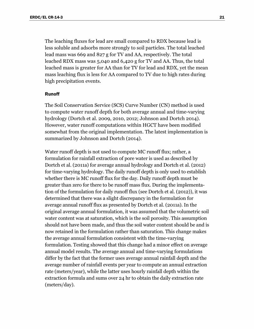
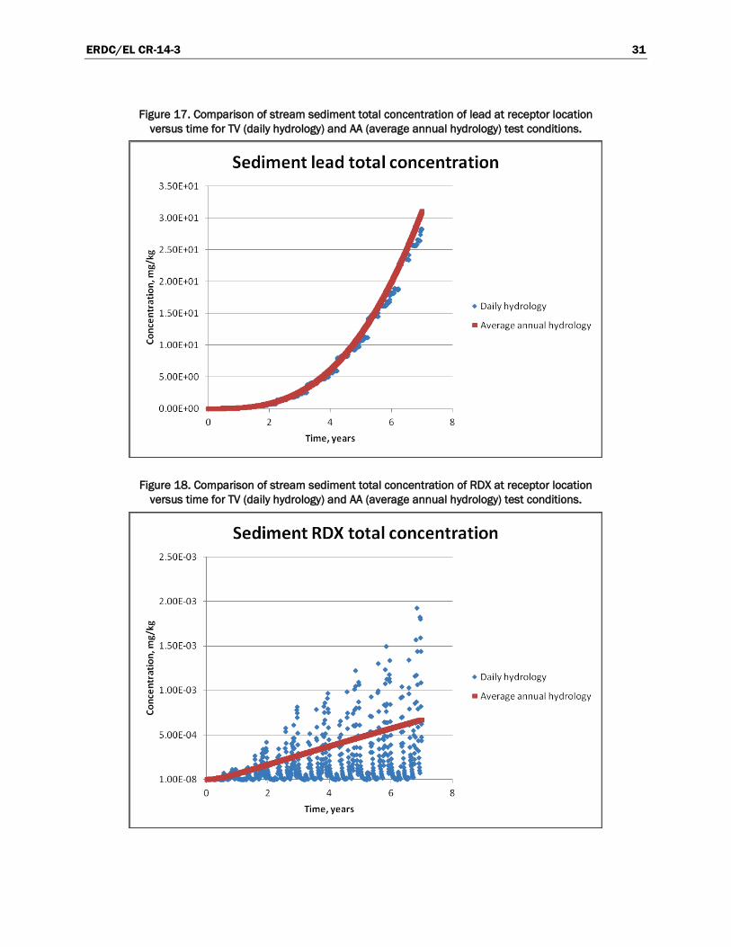
The stream benthic sediment total (pore-water dissolved plus sediment solids adsorbed) concentrations of lead and RDX at the receptor location are plotted versus time in Figures 17 and 18, respectively, for comparison of TV and AA results. The sediment lead concentrations are quite similar for TV and AA. This similarity is due to sediment memory of lead associated with a relatively high sorption distribution coefficient. The stream sediment RDX concentrations for TV are distributed around those for AA with a tendency for TV concentrations to be less than AA concentrations. For TV, sediment concentrations for RDX fluctuate much more than those for lead due to the low sediment memory of RDX associated with its much lower sorption partitioning coefficient. In fact, during periods of low, base flow with no AOI loadings, the sediment concentration of RDX drops three to four orders of magnitude for TV as shown in Figure 19 using log concentration in the plot.
The means of the TV and AA sediment concentrations over the 7 years are, respectively, 7.56 and 7.96 mg/kg for lead and 1.75E-4 and 3.2E-4 mg/kg for RDX. The lead concentration at the end of the 7 years is 28.2 and 31.0 mg/kg for TV and AA, respectively. The ending concentration for RDX is not given since the TV values fluctuate so widely.
Stream water column concentration
CMS outputs water column concentrations in addition to sediment concen-trations over time and space (i.e., distance along the stream). Statements made above regarding input conditions apply. There are some similarities between stream water column and bed sediment concentrations since one is affected by the other due to deposition, resuspension, and mass transfer between sediment pore-water and the water column.
ERDC/EL CR-14-3 31
Figure 17. Comparison of stream sediment total concentration of lead at receptor location versus time for TV (daily hydrology) and AA (average annual hydrology) test conditions.
Figure 18. Comparison of stream sediment total concentration of RDX at receptor location versus time for TV (daily hydrology) and AA (average annual hydrology) test conditions.
ERDC/EL CR-14-3 32
Figure 19. Comparison of stream sediment total concentration of RDX at receptor location versus time for TV (daily hydrology) and AA (average annual hydrology) test conditions (using
log concentration).
The stream water column total (dissolved plus particulate) concentrations of lead and RDX at the receptor location are plotted versus time in Figures 20 and 21, respectively, for comparison of TV and AA results. Both figures exhibit scatter of TV results about the more continuous AA results with a majority of TV concentrations below the AA values. More extreme excursions of TV results below AA results can be observed for RDX.
The means of the TV and AA water column concentrations over the 7 years are, respectively, 2.38E-4 and 2.65E-4 mg/L for lead and 5.98E-5 and 1.07E-4 mg/L for RDX. Results of TV are far more consistent with those of AA for lead than for RDX, which is most likely due to the much higher sorption partitioning coefficients for lead. Higher sorption partitioning leads to greater sediment memory, which results in less water column fluctuation.
Summary
The results presented within this chapter for TV and AA media fluxes and concentrations are summarized in Table 7. Overall, the use of daily rather than average annual hydrology results in less MC mass exported from the
ERDC/EL CR-14-3 33
AOI to receiving surface water and groundwater, which translates into lower receiving water concentrations of MC. Stream water and sediment concentrations of lead for TV and AA compared much closer than they did for RDX probably due to the much tighter binding of lead to sediments.
Figure 20. Comparison of stream water column total concentration of lead at receptor location versus time for TV (daily hydrology) and AA (average annual hydrology) test
conditions.
Figure 21. Comparison of stream water column total concentration of RDX at receptor location versus time for TV (daily hydrology) and AA (average annual hydrology) test
conditions.
ERDC/EL CR-14-3 34
Table 7. Summary of test results.
Measure TV AA Units Ratio, TV / AA
Mean dissolution flux of lead 82,465 65,431 g/year 1.26
Mean dissolution flux of RDX 1,470 1,215 g/year 1.21
Total mass of lead dissolved 5.76E5 6.41E5 g 0.90
Total mass of RDX dissolved 1.01E4 0.99E4 g 1.02
Mean erosion flux of lead 1,444 1,166 g/year 1.24
Mean erosion flux of RDX 6.0 4.0 g/year 1.65
Total mass of lead eroded 1.0E4 1.24E4 g 0.81
Total mass of RDX eroded 35.3 30.3 g 1.17
Mean leaching flux of lead 95.7 77.6 g/year 1.23
Mean leaching flux of RDX 1,150 776 g/year 1.48
Total mass of lead leached 669 827 g 0.81
Total mass of RDX leached 5,040 6,420 g 0.78
Mean runoff flux of lead 31.3 48.6 g/year 0.64
Mean runoff flux of RDX 220 280 g/year 0.79
Total runoff mass of lead 219 519 g 0.42
Total runoff mass of RDX 1,450 2,320 g 0.63
Mean volatilization flux of RDX 0.068 0.23 g/year 0.29
Total mass of RDX volatilized 0.49 1.94 g 0.25
Mean export flux to surface water for lead 1,480 1,220 g/year 1.22
Mean export flux to surface water for RDX 226 283 g/year 0.80
Total mass of lead exported to surface water 1.0E4 1.14E4 g 0.88
Total mass of RDX exported to surface water 1,490 2,350 g 0.64
Mean export flux to aquifer for RDX 30 52.8 g/year 0.57
Peak export flux to aquifer for RDX 99.9 176 g/year 0.57
Total mass of RDX exported to aquifer 4,710 8,300 g 0.57
Mean AOI soil concentration for lead 167 135 mg/kg 1.24
Mean AOI soil concentration for RDX 0.44 0.38 mg/kg 1.14
Ending AOI soil concentration for lead 334 334 mg/kg 1.0
Ending AOI soil concentration for RDX 0.86 0.85 mg/kg 1.0
Mean aquifer well concentration for RDX 2.82E-7 4.94E-7 mg/L 0.57
Peak aquifer well concentration for RDX 1.72E-6 3.03E-6 mg/L 0.57
Mean stream sediment concentration for lead 7.56 7.96 mg/kg 0.95
Mean stream sediment concentration for RDX 1.75E-4 3.20E-4 mg/kg 0.55
Ending stream sediment concentration for lead 28.2 31.0 mg/kg 0.91
Mean stream water column concentration for lead 2.38E-4 2.65E-4 mg/L 0.90
Mean stream water column concentration for RDX 0.6E-4 1.07E-4 mg/L 0.56
ERDC/EL CR-14-3 35
4 Validation Application
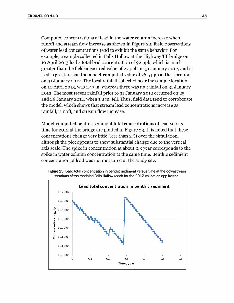
The SAFRs 20–22 at Fort Leonard Wood and the associated Falls Hollow drainage basin, which were used for the testing presented in the previous chapter, were also used for a validation application using time-varying hydrology. This site was previously used as a validation test case using average annual hydrology (Dortch 2013). Most of the model inputs for the present validation application are the same as those of the previous validation application and are described by Dortch (2013). Many of those inputs are also the same as presented in the second chapter of this report since the same site was used for the testing reported herein; differences are described below.
Input modifications
The approach used in the previous validation application was to start the model in 1941, when range use is believed to have started, and project Falls Hollow lead concentrations in 2012, when one stream sample for lead was obtained on 31 January 2012. Lead residue loading within the AOI was computed by TREECS™ based on a constant firing rate each year, which was the average of rates recorded between 1999 and 2012. Model AOI soil lead concentrations were set to zero in 1941. AOI soil and Falls Hollow sediment lead concentrations are directly proportional to firing rates and gradually increase over time as range use continues in the future. The model-computed water total concentration of lead in 2012 was within an order of magnitude of the observed concentration, which is encouraging given the uncertainty in range firing rates (thus MC residue loading rate) over the 72-year period.
The approach for the present validation application was to start the soil model on 1 January 2012, using predicted lead concentrations in 2012 for AOI soil as computed from the previous validation application. It was only necessary to run the model for 1 month since the lead sample was collected on 31 January, but the model was executed for 6 months to capture seasonal effects. Input differences for this application (referred to as the 2012 application) compared to those presented by Dortch (2013) for the original validation are as follows.
ERDC/EL CR-14-3 36
The “starting year of simulation” on the Site Conditions/Operational Inputs screen was changed from 1941 to 2012. The munitions usage information was the same as previously, but this is relatively unimportant since such a short period was simulated.
Hourly precipitation data for 2012 were obtained from NCDC for a station located at the University of Missouri at Rolla, Station COOP237263. These data were processed for input to HGCT. Daily minimum and maximum air temperatures for 2012 were obtained from NCDC for a station located at Fort Leonard Wood, Station USC00232981. The minimum and maximum air temperatures were averaged to estimate mean daily air temperature. The mean and maximum air temperature data were processed into an input file for use with HGCT. HGCT was executed with all other inputs set the same as described by Dortch (2013) except that “time-varying” was used for the analysis type on the Hydrology screen of HGCT UI. The 2012 HGCT results were used to set inputs in the Tier 2 soil model.
There were several changes required for the Tier 2 soil model inputs. The soil-water matrix temperature was set to 15.54 °C rather than 14.17 as in the previous validation application due to different air temperatures in 2012 than for the 61-year record used previously (Dortch 2013). The initial solid and non-solid phase lead concentrations in AOI soil for 2012 were set to 2,881 and 369 mg/kg, respectively, based upon output results from the previous validation application for the year 2012. For the previous validation application, these initial concentrations were set to zero. The output file paths/names from HGCT for time-varying hydrology and hourly precipitation were specified for 2012 on the Hydrology screen of the Tier 2 soil model UI. The time length of simulation was set to 0.5 year for 2012, whereas a 100-year simulation was run previously. All other inputs to the soil model for 2012 were set the same as those for the previous validation application.
Several changes were made to the CMS inputs for 2012 relative to the previous validation application. The maximum time-step of 0.5 day was used, and the total simulation time was set to 0.5 year. A 0.5-day maximum time-step provided a little more resolution and accuracy compared to a 1-day time-step as used for the TV test case, but maximum time-steps less than 0.5 day affected model results only very slightly.
ERDC/EL CR-14-3 37
The initial lead concentration in the sediment bed was changed from zero to 11,300 mg/kg, which was the value computed for 2012 by CMS in the previous validation application after 72 years of simulation. The hydraulic conditions were changed from constant stream width and depth to variable cross-sectional area as a power function of stream flow rate (see Chapter 2 for the TV test case). All other inputs were set the same as for the previous validation application, as well as for the TV test case (see Chapter 2).
Results
The 2012 validation application results are shown in Figure 22 for total concentration of lead in the water column versus time at the downstream terminus of the modeled Falls Hollow reach, which is at the Highway TT bridge or 3.2 km downstream of the SAFRs. The spikes in concentration in the figure are due to storm events. The computed concentration at year 0.085, which is 31 January, is 76.5 µg/L or parts per billion (ppb). The observed lead concentration on that day was 27 ppb. Thus, the computed concentration is almost three times greater than the observed. The computed total concentration of lead in the water column for the original validation, which used average annual hydrology, was 140 ppb (Dortch 2013). Thus, the present application with time-varying hydrology is more accurate than previously with average annual hydrology.
Figure 22. Lead total concentration in water column versus time at the downstream terminus of the modeled Falls Hollow reach for the 2012 validation application.
ERDC/EL CR-14-3 38
Computed concentrations of lead in the water column increase when runoff and stream flow increase as shown in Figure 22. Field observations of water lead concentrations tend to exhibit the same behavior. For example, a sample collected in Falls Hollow at the Highway TT bridge on 10 April 2013 had a total lead concentration of 92 ppb, which is much greater than the field-measured value of 27 ppb on 31 January 2012, and it is also greater than the model-computed value of 76.5 ppb at that location on 31 January 2012. The local rainfall collected near the sample location on 10 April 2013, was 1.43 in. whereas there was no rainfall on 31 January 2012. The most recent rainfall prior to 31 January 2012 occurred on 25 and 26 January 2012, when 1.2 in. fell. Thus, field data tend to corroborate the model, which shows that stream lead concentrations increase as rainfall, runoff, and stream flow increase.
Model-computed benthic sediment total concentrations of lead versus time for 2012 at the bridge are plotted in Figure 23. It is noted that these concentrations change very little (less than 2%) over the simulation, although the plot appears to show substantial change due to the vertical axis scale. The spike in concentration at about 0.3 year corresponds to the spike in water column concentration at the same time. Benthic sediment concentration of lead was not measured at the study site.
Figure 23. Lead total concentration in benthic sediment versus time at the downstream terminus of the modeled Falls Hollow reach for the 2012 validation application.
ERDC/EL CR-14-3 39
Discussion
Several sensitivity runs were made with CMS to gain a better understanding of the importance of various input variables. The TSS concentration for Falls Hollow was not measured and is expected to vary as flow rate varies. Thus, TSS was increased from 9 to 100 mg/L. The order of magnitude increase in TSS resulted in an order of magnitude increase in the base flow water column concentration of lead. The spikes in concentration during storm flow increased very little if at all.
It is noteworthy that the benthic sediment resuspension rate used in CMS was a constant value of 3.77E-5 m/day based on a steady-state solids balance with a TSS settling rate of 1.0 m/day and benthic sediment burial rate of essentially zero (1.0E-20 m/day). This amount of resuspension has a profound effect on water column lead concentrations during low, base flow conditions. With a zero resuspension rate, the water column lead concentration dropped two orders of magnitude from 76.5 ppb to 0.79 ppb on 31 January. The concentration spikes shown in Figure 22 did not change. It is likely that there is little to no resuspension during low flows and high resuspension during high flow events.
The sediment-water partitioning, distribution coefficient for suspended solids was decreased from 500,000 L/kg to 40,000 L/kg, which is the value used for the benthic sediments. This change increased base flow water column concentrations of lead from 76.5 to 103 ppb. Concentration spikes also increased. An order of magnitude decrease in partitioning resulted in less than an order of magnitude increase in water column concentrations. Thus, the partition coefficient is not as sensitive as the input values for TSS and resuspension rate.
The initial concentration of lead in benthic sediments was decreased by almost a third from 11,300 to 4,000 mg/kg. The TSS concentration, the TSS partitioning coefficient for lead, and the resuspension rate were reset to the original values. The decrease in initial sediment concentration of lead resulted in the same amount of decrease in water column concentration of lead for 31 January. The concentration decreased from 76.5 to 27.2 ppb, where 27.2 ppb is very close to the observed value of 27 ppb on that date. This sensitivity run clearly shows the importance of either knowing or accurately estimating the initial sediment concentration of lead. It is possible that the predicted benthic, sediment lead concentration of 11,300 mg/kg exceeds the actual concentration since firing rates over the previous
ERDC/EL CR-14-3 40
72 years were estimated based upon recent firing rates. Sediment concentrations are directly and linearly related to firing rates. Thus, firing rates over the 72-year period may have been overestimated. It is unfortunate that benthic sediment lead concentration was not measured for comparison to that predicted. Benthic sediments provide long-term memory of contaminant loadings and do not exhibit the wide temporal concentration fluctuations associated with the water column. Therefore, it is good practice to measure benthic concentrations when obtaining water column concentrations.
Several modeling limitations can contribute to inaccuracy in computed stream concentrations of lead. While the CMS assumes a constant background water flow rate, background flows vary during storms. Background flow in this case is all flow entering the stream that does not originate from the AOI. Thus, background flow for Falls Hollow can be comparable to or possibly larger than flow from the AOI. Variable background flow can have a varying dilution effect on lead loading fluxes from the AOI to the stream. This model limitation is addressed further in the next chapter.
Another limitation of the CMS is the assumption of constant, user-specified TSS concentration. It was demonstrated that TSS concentration has a profound effect on lead concentrations in the stream. Additionally, TSS is expected to vary with water flow rate. Also, as noted above, the use of a constant resuspension rate and the associated value can have a major effect on computed water column concentrations during low flow conditions. These model limitations are also addressed further in the next chapter.
ERDC/EL CR-14-3 41
5 Recommendations
Application of the time-varying (daily) hydrology feature within TREECS™ should provide more accurate predictions of MC fate than does the use of average annual hydrology. The use of daily hydrology results in lower receiving water concentrations of MC than does the use of average annual hydrology. Thus, using average annual hydrology provides more conservative predictions for MC concentrations at receptor locations.
The MEPAS vadose and aquifer models have a time-step limitation. The model time-step is computed internally using 240 total time-steps over the simulation period. The simulation period for these two models is also determined internally to ensure capturing the entire contaminant flux/concentration history, which starts near zero, peaks, and returns to near zero. The 240-step limitation has resulted in less than desirable accuracy and model execution failure for some cases. It is recommended that the MEPAS vadose and groundwater models be modified to allow the user to increase or change the number of time-steps.
When surface water is a receptor medium of interest, CMS should be applied since the other surface water model within TREECS™ (i.e., the RECOVERY model) is not appropriate for time-varying flows. The RECOVERY model is more appropriate for standing surface water, such as lakes, ponds, etc., and employs steady-state conditions for flow and depth. This model could be modified to handle time-varying flows and depth, but such modifications are beyond the present scope of study. The RECOVERY model can also fail to execute when contaminant loadings fluctuate widely between zero and nonzero values. This latter problem is caused by the automatic time-step feature within the model. Thus, if the time-varying hydrology feature is selected, only CMS should be used at this time.
Computer processing time should be considered when applying CMS. For example, a 7-year simulation with CMS for the TV case using a 1-day time-step required 8 minutes on an Intel Xeon 2.7 GHz processor with a 64-bit operating system and 16 GB of internal memory. It is not unusual to require simulations of 100 years or longer for evaluating MC fate down-gradient of firing ranges. Such runs would require approximately 2 hr. Long execution times become prohibitive when trying to conduct sensitivity and uncertainty
ERDC/EL CR-14-3 42
analyses with the Monte Carlo simulation feature within TREECS™, which requires many simulations. The use of average annual hydrology is recommended for long-term simulations and for applications utilizing sensitivity and uncertainty analyses. Daily hydrology can be used to provide a final refinement of a long-term simulation.
A time-step of a day or less should be used in CMS when run with daily hydrology. If not, inaccurate and erroneous results can be produced. CMS presently writes output at a frequency that is approximately double the time-step. An option to control the write frequency should be considered.
Two upgrade features are recommended for CMS, one of which involves stream-water flow. CMS presently allows two types of water flows to enter the stream system, a background flow of a constant rate and a loading flow that can have time-varying rates. Both flows enter at the most upstream computational segment. The loading flow is generated by the soil model and represents runoff and soil interflow from the AOI. The loading flow can also include groundwater discharge to surface water. In many cases, the watershed feeding the receiving stream is larger than the AOI watershed; in other words, the AOI is within a sub-watershed of the larger watershed that feeds the stream. A more realistic representation would be to allow background flows that vary from a low, base flow to large storm flows generated over the entire watershed. The storm flows can be generated by simply multiplying the daily runoff depth by the stream watershed area. There should also be an option to distribute background flows among model segments rather than having to place all in the most upstream segment.
The other CMS upgrade involves time-varying TSS and resuspension. The stand-alone version of CMS has the option to simulate variable TSS transport with settling and variable resuspension, where resuspension is computed based on flow conditions. As discussed in the previous chapter, TSS and resuspension have a profound effect on computed MC stream concentrations. TSS and resuspension normally increase as stream flow rate increases. These features should be implemented in the TREECS™ version of CMS.
The hydrology model within the HGCT was modified to allow the option for providing average annual or time-varying (daily) hydrologic output. However, both options compute daily volumetric soil water content and
ERDC/EL CR-14-3 43
infiltration using the latest soil water balance procedure detailed in Appendix A of this report. Prior to these modifications, the soil water content was not computed, rather it was assumed to be equal to the field capacity for hydrology computations. It is now possible to use the computed and more accurate soil water content for the average annual hydrology by simply averaging the computed daily values for the period of record and automatically providing this value to the Tier 2 soil model. The hydrology model must be modified to reflect this improved feature as well as the HGCT and the soil model UI. Values of daily soil water content are provided to, and used by, the soil model when the time-varying hydrology options are selected in HGCT and the soil model UIs.
ERDC/EL CR-14-3 44
6 Conclusions
A time-varying hydrology feature has been implemented into TREECS™ as an alternative to using average annual hydrology. This new feature required new options within HGCT and the Tier 2 soil model. When this feature is used, daily values are generated by HGCT for AOI precipitation runoff depth, soil water content, infiltration depth, and soil erosion depth for use in the soil model. The soil model generates daily fate and export fluxes for MC. The MEPAS vadose and aquifer models can process daily varying loadings from the soil model, but due to a time-step limitation, there were cases where the models failed to execute. The CMS handled daily loadings from the soil model with no problems. The RECOVERY surface water model cannot handle daily loadings from the soil model without modifications. Overall, the daily hydrology feature is best suited for surface water analyses using CMS, and this new feature performed reasonably well for that case.
Testing of TREECS™ with daily hydrology was performed by running the same site conditions for two test conditions, one with average annual hydrology (AA) and one with time-varying (daily) hydrology (TV), and comparing the two. These tests showed that TV performed well compared to AA where all fluxes and concentrations for TV bounded those for AA while exhibiting broader fluctuations. AOI soil export mass fluxes to surface water and groundwater were less for TV compared to AA. Lower export mass fluxes resulted in lower receiving water and sediment mean concentrations for TV compared to AA. Evidently, intermittent precipitation, spaced between dry periods, results in less export than the constant, continuous precipitation associated with using average annual hydrology. As a result, the use of average annual hydrology produces more conservative results than daily hydrology.
A validation application for SAFRs that drain into Falls Hollow at Fort Leonard Wood was performed using daily hydrology for the year 2012. The initial soil and sediment concentrations for this application were set to those predicted from a previous Falls Hollow application described by Dortch (2013). The model-computed total concentration of lead in the water column was 2.8 times greater than that observed on 31 January 2012. One of the potential reasons for this error is inaccurate predictions
ERDC/EL CR-14-3 45
of stream benthic sediment concentrations of lead for 2012 from the previous Falls Hollow application. The model predictions for benthic sediment lead concentration were based on rough estimates of range firing rates over a 72-year period preceding 2012. Firing rate estimates may have been inflated. Additionally, simplifying model assumptions built within the CMS, such as constant TSS, resuspension rate, and base flow, could also contribute to model error. Measured lead concentrations in benthic sediments are needed to provide an improved understanding of model performance and accuracy.
It is concluded that the daily hydrology feature will be most useful for applications involving short periods (1 year or less) to evaluate the effects of variable precipitation and flow on MC concentrations in streams. The upgrades recommended for CMS can provide increased accuracy for such applications.
ERDC/EL CR-14-3 46
References Dortch, M. S., J. A. Gerald, and B. E. Johnson. 2009. Methods for Tier 1 modeling with
the Training Range Environmental Evaluation and Characterization System. Technical Report ERDC/EL TR-09-11. Vicksburg, MS: U.S. Army Engineer Research and Development Center.
Dortch, M. S., B. E. Johnson, and J. A. Gerald. 2010. Proof-of-concept application of Tier 1 modeling approach within the Training Range Environmental Evaluation and Characterization System. Technical Report ERDC/EL TR-10-19. Vicksburg, MS: U.S. Army Engineer Research and Development Center.
Dortch, M. S., B. E. Johnson, Z. Zhang, and J. A. Gerald. 2011a. Methods for Tier 2 Modeling within the Training Range Environmental Evaluation and Characterization System. Technical Report ERDC/EL TR-11-2. Vicksburg, MS: U.S. Army Engineer Research and Development Center.
Dortch, M. S., B. E. Johnson, J. A. Gerald, Z. Zhang, and A. P. Simmons. 2011b. Proof-of-Concept Application of Tier 2 Modeling Approach within the Training Range Environmental Evaluation and Characterization System. Technical Report ERDC/EL TR-11-10. Vicksburg, MS: U.S. Army Engineer Research and Development Center.
Dortch, M. S., B. E. Johnson, Z. Zhang, and J. A. Gerald. 2012. Extension of capabilities for the Tier 1 and Tier 2 approaches within the Training Range Environmental Evaluation and Characterization System (TREECS™). Technical Report ERDC/EL TR-12-11. Vicksburg, MS: U.S. Army Engineer Research and Development Center.
Dortch, M. S. 2013. Application of TREECS to small arms firing ranges at Fort Leonard Wood, MO. ERDC/TN EQT-13-2. Vicksburg, MS: U.S. Army Engineer Research and Development Center.
Haan, C. T., B. J. Barfield, and J. C. Hayes. 1994. Design hydrology and sedimentology for small catchments. San Diego, CA: Academic Press, Inc.
Johnson, B. E., and M. S. Dortch. 2014. Formulation of the hydrology model within the Training Range Environmental Evaluation and Characterization System. 2014. ERDC/EL TR-14-2. Vicksburg, MS: U.S. Army Engineer Research and Development Center.
Ponce, V. M. 1989. Engineering hydrology, principles and practices. Upper Saddle River, NJ: Prentice-Hall, Inc.
Williams, J. R. 1975. Sediment-yield prediction with Universal Equation using runoff energy factor. In Present and Prospective Technology for Predicting Sediment Yield and Sources. ARS-S-40, 244-252. U.S. Department of Agriculture.
ERDC/EL CR-14-3 47
Appendix A: Summary of Methods for Computing Time-Varying Water Balance and Erosion for Surface Soil
The methods used within the hydrology model of HGCT for computing soil hydrology, including runoff, evapotranspiration (ET), and infiltration, are described in the report by Johnson and Dortch (2014).1 However, the latest version of the hydrology model uses a revised method for computing the soil water balance. This revised method considers daily soil water content for computing ET and infiltration. This revised method, which is used for both the average annual and daily hydrology options, is described in this appendix.
The time-varying hydrology feature within the HGCT of TREECS™ uses MUSLE for computing daily soil erosion. This approach is described in this appendix along with the TR55 method for computing the peak runoff rate, which is needed in MUSLE.
Water balance
Infiltration rate I within TREECS™ is the soil water loading rate available for percolation and/or soil interflow. For this reason, I can also be referred to as the infiltration capacity. The formula for estimating the infiltration rate in the original version of the HGCT hydrology model was
I P Q ET (A1)
where I, P, Q, and ET are the average annual infiltration, precipitation, runoff, and actual evapotranspiration rates (meters/year), respectively. Equation A1 is based on the assumption of a constant soil water content that is at field capacity.
Daily runoff is computed within the HGCT hydrology model using a modified curve number method as described by Johnson and Dortch (2014). Monthly potential evapotranspiration (PET) is computed using an
1 References cited in this appendix can be found in the References section following the main text.
ERDC/EL CR-14-3 48
air temperature approach (Johnson and Dortch 2014). Daily values of PET are the monthly value divided by the number of days in the month.
The hydrology model was modified to include daily varying soil water content based on a soil water balance, which is described as follows. The infiltration rate for any given day t can be computed from the excess water content above the field capacity as follows:
, .t t FCI Max θ θ H 1 0 0 (A2)
where θt-1 is the volumetric soil water content (fraction) for the previous day, θFC is the soil field capacity (fraction), and H is the soil layer thickness, which will cancel out of the system of equations. The field capacity is a constant that depends on soil texture. Similarly, the ET for any given day t can be computed from
,t t r tET Min θ θ H PET 1 (A3)
where θr is the soil residual water content (fraction). With values for It and ETt, the water content can be updated from a soil water balance,
,t t t tt t r
P Q ET Iθ Max θ θ
H
1 (A4)
The daily precipitation is an input, and the daily runoff Qt has been computed from the curve number method before applying Equation A4. The water content for the present day (θt) becomes the water content for the previous day during the next daily update.
The above approach is an approximation since it is assumed that ET is independent of I, P, and Q for the day. This assumption allows a direct solution for daily updates without any iteration. Thus, this solution approach is referred to as an explicit solution.
A more correct approach, which requires an iterative solution, is available within the hydrology model. This approach includes the full water balance for computing ET as follows,
,t t r t t t tET Min θ θ H P Q I PET 1 (A5)
ERDC/EL CR-14-3 49
As before, the water content for the day is updated using Equation A4. However, Equations A4 and A5 include the infiltration rate for the day. The daily infiltration is more accurately determined using an average of the water content for the beginning and end of the day as follows:
, .t tt FC
θ θI Max θ H
1 0 02
(A6)
The subscript t-1 represents the value for the previous day, which is the same as the beginning of day t; and subscript t represents the value for the present day, which is the same as the end of day t. Equations A4–A6 are three equations with three unknowns that are solved iteratively with convergence criteria set on It. At time zero, the water content is assumed to be at field capacity. An initial value of It is required for each time-step, and this value is obtained using Equation A2. Equations A4 and A5 are solved using the initial value of It, and then It is updated with Equation A6. This solution cycle continues until convergence for It has been reached. This iterative solution approach is referred to as an implicit solution. Testing has shown that the use of the implicit solution option is preferred since it converges rapidly and provides a more accurate water balance. The daily solution for soil water content with the explicit and implicit options are employed for both the average annual and time-varying hydrology options within the HGCT.
Soil erosion
The Modified Universal Soil Loss Equation (MUSLE) is used to estimate daily soil erosion rates. The MUSLE equation (Williams 1975) is stated as
..s v pA Q Q K LS C P
0 5611 8 (A7)
where
As = sediment yield from overland soil erosion for a rainfall event, metric tons (MT)
Qv = event runoff volume, m3
Qp = peak runoff flow rate for an event hydrograph, m3/sec
ERDC/EL CR-14-3 50
The other parameters in Equation A7 (K, LS, C, P) are the standard USLE parameters that are used in the HGCT of TREECS™. In this implementa-tion of MUSLE, an event is defined as daily rainfall.
The steps required for estimating the two flow variables in Equation A7 are as follows.
1. The daily runoff volume Qv is computed by the HGCT hydrology model by multiplying the daily runoff depth by the catchment (i.e., AOI) surface area. It is noted that the hydrology model can compute runoff without rainfall due to snow melt.
2. The daily peak runoff flow rate Qp is estimated by the HGCT using the SCS TR-55 method as outlined below.
3. With values for Qp and Qv, the MUSLE equation is applied within the HGCT to compute sediment yield for each day (metric tons/day; one metric ton = 1,000 kg). The sediment yield is divided by the AOI surface area (square meters), and that result is divided by the soil dry bulk density ρb (metric tons per cubic meter) to obtain the erosion rate E (meters/day). Soil dry bulk density is estimated by the HGCT based on soil composition and is approximately 1.5 MT/m3.
The SCS TR-55 method for computing the peak flow rate of runoff from a rainfall event is described by Ponce (1989) and Haan et al. (1994). This approach does not extend to snow melt. Thus, if there is no rainfall for the day, Qp is set to zero, and sediment yield is zero. In the TR-55 method, the runoff peak flow rate Qp (cubic feet per second, cfs) is computed from
p u roQ q A F H (A8)
where qu is the runoff unit peak flow rate (cfs/square mile/inch), A is the catchment surface area (square miles), F is the surface storage correction factor (unit-less), and Hro is the runoff depth (inches) for the event. The runoff depth for each day is computed by the hydrology model within HGCT as described by Johnson and Dortch (2014). The peak flow rate determined from Equation A8 must be converted to cubic meters/second for use in Equation A7.
The unit peak flow rate qu depends on the type of 24-hr temporal rainfall distribution, the ratio of the initial abstraction to the event rainfall, Ia/P, and the catchment time of concentration tc for flow at the basin outlet. For
ERDC/EL CR-14-3 51
this implementation of TR-55, the duration of each event is a day; thus, the event rainfall is the rainfall depth for the day. The initial abstraction is computed from the daily retention capacity S and the previous day’s rainfall depth as described by Johnson and Dortch (2014).
The time of concentration (hours) can be estimated using the Hathaway formula as described by Ponce (1989)
.
.
.c
c
Lnt
S
0 467
0 234
0 606 (A9)
where L is the length (km) of the principal water course of the basin from outlet to divide (i.e., upstream extent of the AOI draining towards the outlet), Sc is the slope (unit-less) between maximum and minimum elevation of the catchment water course, and n is a roughness factor. The roughness factor varies between 0.02 for smooth, impervious surfaces to 0.8 for timber land with deep litter. The values for bare soil, poor grass, and pasture are about 0.1, 0.2, and 0.4, respectively. Thus, it is expected that values for impact areas of large and medium caliber munitions would be approximately the same as poor grass, or about 0.2. The roughness factor is an input specified by the user.
The four types of SCS rainfall distributions for the United States are shown in Figure A1. The locations of each type of rainfall distribution are shown in Figure A2. The user must specify the rainfall distribution type.
Figure A1. SCS 24-hr rainfall distribution (from Ponce (1989)).
ERDC/EL CR-14-3 52
Figure A2. SCS 24-hr rainfall distribution map (from Ponce (1989)).
The unit peak runoff flow rate can be determined (Haan et al. 1994) from
log log logu o c cq C C t C t 2
1 2 (A10)
The three coefficients in Equation A10 depend on the rainfall type and Ia/P, and can be found in Table A1. With the three coefficients and an estimate of tc, qu can be calculated from Equation A10.
Table A1. Coefficients for runoff peak unit discharge equation (from Haan et al. (1994)).
Rainfall Type Ia/P C0 C1 C2
I 0.1 2.3055 -0.51429 -0.1175
0.2 2.23537 -0.50387 -0.08929
0.25 2.18219 -0.48488 -0.06589
0.3 2.10624 -0.45695 -0.02835
0.35 2.00303 -0.40769 0.01983
0.4 1.87733 -0.32274 0.05754
0.45 1.76312 -0.15644 0.00453
0.5 1.67889 -0.0693 0
IA 0.1 2.0325 -0.31583 -0.13748
0.2 1.91978 -0.28215 -0.0702
0.25 1.83842 -0.25543 -0.02597
0.3 1.72657 -0.19826 0.02633
0.5 1.63417 -0.091 0
ERDC/EL CR-14-3 53
Rainfall Type Ia/P C0 C1 C2
II 0.1 2.55323 -0.61512 -0.16403
0.3 2.46532 -0.62257 -0.11657
0.35 2.41896 -0.61594 -0.0882
0.4 2.36409 -0.59857 -0.05621
0.45 2.29238 -0.57005 -0.02281
0.5 2.20282 -0.51599 -0.01259
III 0.1 2.47317 -0.51848 -0.17083
0.3 2.39628 -0.51202 -0.13245
0.35 2.35477 -0.49735 -0.11985
0.4 2.30726 -0.46541 -0.11094
0.45 2.24876 -0.41314 -0.11508
0.5 2.17772 -0.36803 -0.09525
The surface storage correction factor F depends on the percent of ponding within the catchment as shown in Table A2. The percentage of ponding is input by the user. Given the above data, there is now enough information to compute Qp from Equation A8.
Table A2. Surface storage correction factor.
Percentage of ponds and swamps F
0 1.0
0.2 0.97
1 0.87
3 0.75
5 0.72
Steps 2 and 3 above in the MUSLE computation are performed by the HGCT module, so there are four new inputs in HGCT for AOI soil erosion. These include: AOI water course length L; the SCS storm type; AOI runoff surface roughness factor n; and percent of AOI ponding.
For confirmation, the above procedure for computing daily erosion was compared to the USLE results calculated for the AOI at Fort A.P. Hill (Dortch et al. 2011b) without using the sediment delivery ratio, SDR ( i.e., SDR was set to 1.0). Values of the USLE input parameters were used for MUSLE, which included K = 0.24, Sc = 0.06 with runoff length of 400 ft or greater, C = 0.1, P = 1.0. Additionally, the following inputs were provided for
ERDC/EL CR-14-3 54
the MUSLE application: A = 4.16 square miles = 10,775,905 m2 = 10.78 km2; L = 2.285 km; storm type II for Virginia; n = 0.2; and percent ponding = 1.0.
The daily erosion rates computed with MUSLE for the above inputs were summed for each day over the 26 years for the input precipitation record and then divided by 26 to obtain an average annual rate. The rates are compared here as fluxes in U.S. mass units (tons, T, or 2000 pounds) per unit area (acre) per year. The average annual flux computed with MUSLE using daily rainfall was 7.94 T/acre/year, and the flux computed using USLE was 7.21 T/acre/year. This excellent agreement provides confidence that the methods for computing daily erosion with MUSLE were properly formulated and implemented.
It is noted that MUSLE depends on four new inputs that USLE does not use, and USLE has the rainfall factor R, which MUSLE does not use. The storm type II is appropriate for the location of Fort A.P. Hill, so this input was not varied for sensitivity. The percent of ponding was increased to 5%, which had essentially no effect on the average annual erosion rate computed with MUSLE. The AOI area can affect MUSLE results, but it is assumed that the area is known and should not be varied for sensitivity. The two remaining MUSLE inputs, n and L, are uncertain, so they were varied for sensitivity. It is expected that n could be as high as 0.3 rather than 0.2. The value used for L is the linear, straight-line, and longitudinal extent of the AOI along the flow gradient. It is expected that the actual flow path could be longer by as much as 10 to 20%. Thus, another MUSLE calculation was conducted with the same inputs as before except with n = 0.3 and L = 2.5 km. These changes resulted in a MUSLE-computed, average, annual erosion rate of 7.34 T/acre/year, which compares more closely with the value of 7.21 T/acre/year computed with USLE.
A much simpler approach than TR-55 for estimating runoff peak flow rate was tested prior to testing the TR-55 approach. This simpler approach consisted of assuming a triangular runoff distribution such that the runoff volume for the day Qv was the area under a triangle with base td and height Qp, where td is the duration of the rainfall for the day. Thus, the estimation
for daily maximum runoff flow rate was computed from vp
d
QQ
t
2 . This
approach resulted in a MUSLE-computed, average annual erosion rate of 5.23 T/acre/year, which is considerably less than the USLE estimate. Thus, the decision was made to implement the TR-55 approach into the MUSLE computations within HGCT.
REPORT DOCUMENTATION PAGE Form Approved OMB No. 0704-0188
Public reporting burden for this collection of information is estimated to average 1 hour per response, including the time for reviewing instructions, searching existing data sources, gathering and maintaining the data needed, and completing and reviewing this collection of information. Send comments regarding this burden estimate or any other aspect of this collection of information, including suggestions for reducing this burden to Department of Defense, Washington Headquarters Services, Directorate for Information Operations and Reports (0704-0188), 1215 Jefferson Davis Highway, Suite 1204, Arlington, VA 22202-4302. Respondents should be aware that notwithstanding any other provision of law, no person shall be subject to any penalty for failing to comply with a collection of information if it does not display a currently valid OMB control number. PLEASE DO NOT RETURN YOUR FORM TO THE ABOVE ADDRESS. 1. REPORT DATE (DD-MM-YYYY) August 2014
2. REPORT TYPE Final report
3. DATES COVERED (From - To)
4. TITLE AND SUBTITLE
Evaluation of Time-Varying Hydrology within the Training Range Environmental Evaluation and Characterization System (TREECS™)
5a. CONTRACT NUMBER
5b. GRANT NUMBER
5c. PROGRAM ELEMENT NUMBER
6. AUTHOR(S)
Mark S. Dortch
5d. PROJECT NUMBER
5e. TASK NUMBER
5f. WORK UNIT NUMBER
7. PERFORMING ORGANIZATION NAME(S) AND ADDRESS(ES) 8. PERFORMING ORGANIZATION REPORT NUMBER
Los Alamos Technical Associates, Inc. 999 Central Avenue, #300 Los Alamos, NM 87544
U.S. Army Corps of Engineers Washington, DC 20314-1000
11. SPONSOR/MONITOR’S REPORT NUMBER(S)
12. DISTRIBUTION / AVAILABILITY STATEMENT
Approved for public release; unlimited distribution.
13. SUPPLEMENTARY NOTES 14. ABSTRACT The Training Range Environmental Evaluation and Characterization System (TREECS™) uses average annual hydrologic conditions as inputs for multi-media fate and transport models. This simplification reduces model complexity and data input requirements while providing the capability to conduct long-term predictions of the fate of munitions constituents (MC) as well as other contaminants. TREECS™ was recently modified to allow the option of using time-varying (daily) hydrology for forcing input conditions. This report summarizes the results of testing this new feature. MC fate predictions with daily hydrology are compared with those using average annual hydrology. Results show that the use of average annual hydrology produces more conservative results (i.e., higher media concentrations) than using daily hydrology. A validation application for lead downstream of small arms firing ranges is also presented in this report. The daily hydrology feature will be most useful for applications involving short periods (year or less) to evaluate the effects of variable precipitation and flow on MC concentrations in streams.
15. SUBJECT TERMS Fate modeling of munitions constituents Groundwater models
Surface water Soil Time-varying, daily hydrology
16. SECURITY CLASSIFICATION OF: 17. LIMITATION OF ABSTRACT