Introduction to differential algebraic geometryand differential algebraic groupsNovember 4, 18, December 2, 9, 2005

In his 1979 article on nonlinear differential equations, Manin describesthree possible languages for the variational formalism: the classical lan-guage, the geometric language, and, differential algebra. He critiques eachapproach. He writes:

The language of differential algebra is better suited for ex-pressing such properties (invariant properties of differential equa-tions), and, puts at the disposal of the investigator the exten-sive apparatus of commutative algebra, differential algebra, andalgebraic geometry....The numerous “explicit formulas” for thesolutions of the classical and newest differential equations havegood interpretations in this language; the same may be said forconservation laws. However, the language of differential alge-bra which has been traditional since the work of Ritt does notcontain the means for describing changes of the functions (depen-dent variables) and the variables xi (independent variables), andfor clarifying properties which are invariant under such changes.This is one of the main reasons for the embryonic state of so-called “Backlund transformations” in which there has been a re-cent surge of interest.

The development of differential algebraic geometry, which began in the1970’s has begun to address these concerns. There is a lot left to do. Fora modern approach, see Kovacic (2002 ff)

1 Differential Algebraic Geometry

Throughout, F is a differential field of characteristic 0, equipped with a set∂ of commuting derivation operators ∂1, . . . , ∂m, and, field C of constants.Note that the field Q of rational numbers is contained in C. Let Θ be thefree commutative monoid on ∂. If θ = ∂k11 · · · ∂kmm is a derivative operator inΘ, then, ordθ =

Pki. If the cardinality of ∂ is 1, we identify the set with

its only element, and, call F an ordinary differential field . Otherwise, F is

1

a partial differential field. Throughout, we will use the prefix ∂- in place of“differential” or “differentially.”Note that we define the ∂-structure on an F-algebra R by a homomor-

phism from Θ into the multiplicative monoid (EndR,·) that maps ∂ intoDerR. If S is a ∂-ring and a subring of a ∂-ring R, then, the ∂-structure ofR extends that of S. In particular, the action of ∂ on R extends the actionof ∂ on F. We call R a ∂-F-algebra. All our ∂-rings will be ∂-F-algebras.If R is a ∂-F-algebra, a = (a1, . . . , an) is a finite family of elements of

R, and θ ∈ Θ, we denote by θa the family (θa1, . . . , θan), and, by Θa thefamily θa, θ ∈ Θ. R is finitely ∂-generated over F if there exists a finitefamily a of elements of R such that R = F [Θa]. We write R = F {a} =F {a1, . . . , an}. If y = (y1, . . . , yn) is a family of ∂-indeterminates, then, the∂-polynomial algebra F {y} = F {y1, . . . , yn} over F is, thus, an infinitelygenerated polynomial algebra over F. We can think of the ∂-polynomials asfunctions on Fn.If G is a ∂-extension field of F, G is finitely ∂-generated over F if there

exists a finite family a of elements of G such that G = F (Θa). We writeG = F hai. G is the quotient field of R = F {a}.Example 1.1. Let D be a connected open region of Cm, C the field of com-plex numbers, and, let t1, . . . , tm be complex variables. Set ∂ = {∂t1, . . . , ∂tm}.Let G = (G, ∂) be the ∂-field of functions meromorphic in D. Let F = (F, ∂)be the ∂-field of functions meromorphic in Cm. Then, G is a ∂-extensionfield of F.

Let R, and, S be ∂-algebras over F. An F-algebra homomorphism ϕ :R→ S is a ∂-homomorphism if ϕ◦∂i = ∂i◦ϕ (ϕ commutes with the action ofthe derivation operators.) kerϕ is a ∂-ideal of R, and im ϕ is a ∂-subalgebraover F of S.

Theorem 1.2. The Seidenberg Lefschetz Principle (1958). Let F beany ∂-field that is finitely ∂-generated over Q, where ∂ = {∂1, . . . , ∂m}. Let(M, ∂) be the field of meromorphic functions on Cm, where the action of ∂ isby the partial derivatives of the complex variables t1, . . . , tm. Then, there isa connected open region D of Cm and, a ∂-isomorphism of F into the fieldof meromorphic functions on D.

The logician Abraham Robinson formulated the analogue for differentialalgebra of an algebraically closed field (1959). Let f1, . . . , fr, g be differential

2

polynomials of positive degree in F {y1, . . . , yn}. The systemf1 = 0, . . . , fr = 0, g 6= 0

is consistent if there exists a ∂-extension field G of F and a family a =(a1, . . . , an) of elements of G such that f1(a) = 0, . . . , fr(a) = 0, g(a) 6= 0.F is differentially closed if every consistent system of differential polynomialequations and inequations has a solution with coordinates in F. A differen-tially closed differential field is algebraically closed.

1.1 Differential affine n-space An: The Kolchin topol-ogy

Let U be a differentially closed ∂-extension field of F. Let K be the fieldof constants of U. Recall the Zariski topology on Un: V ⊂ Un is Zariskiclosed if there exist polynomials (fi)i∈I , fi ∈ U[y1, . . . yn] such that V ={a ∈ Un : fi(η) = 0, i ∈ I}. The Zariski closed sets are the closed sets ofthe topology.whose closed sets are algebraic varieties. Now assume thaty1, . . . , yn are ∂-indeterminates over U.Using the Zariski topology as a model, we define the Kolchin topology on

Un. A subset V of Un is Kolchin closed if there exist ∂-polynomials (fi)i∈I ,fi ∈ U{y1, . . . yn} such that V = {a ∈ Un : fi(a) = 0, i ∈ I}. The closedsets in the Kolchin topology are also called ∂-varieties. If the differentialpolynomials defining V have coefficients in F, we say V is defined over F,and call it a ∂-F-variety.If V is the set of zeros of fi, i ∈ I, then, V is the set of zeros of the ∂-ideal

i = [(fi)i∈I ] that they generate. We denote V by V (i). Conversely, if i is a∂-ideal of U{y1, . . . yn}, V = V (i) is Kolchin closed.Note that V is order reversing:

i ⊂ j⇒ V (i) ⊃ V (j)Also,

V ([1]) = ∅V ([0]) = Un

V (i ∩ j) = V (ij) = V (i) ∪ V (j)V (i+ j) = V (i) ∩ V (j)

3

We denote Un, equipped with the Kolchin topology by the symbol An.If V is a Kolchin closed subset of Un, V is a topological space in the inducedtopology.Every Zariski closed set is Kolchin closed, but, not conversely. The

Kolchin topology is a much larger topology than the Zariski topology. For ex-ample, every Zariski closed subset of A1 is finite, whereas non—finite Kolchinclosed subsets abound. Indeed, there are strictly increasing chains of Kolchinclosed subsets: If U is ordinary, with derivation operator, ∂, and, x ∈U has derivative 1, we have the chain {0} = V ([y]) ⊂ K = V ([∂y]) ⊂{ax+ b : a, b ∈ K} = V ([∂2y]) ⊂ {ax2 + bx+ c : a, b, c ∈ K}= V ([∂3y]) ⊂ ....Exercise 1.3. Prove that if U is an ordinary ∂-field, X = {p (x) : p(x) apolynomial with coefficients in K} is not Kolchin closed in A1.

Note: V³√i´= V (i). E.G., in U {y}, V ([y2]) = {0} = V

³p[y2]´=

V ([y]).Call two systems of differential equations equivalent if they have the same

solutions. An important motivation for Ritt in his development of differen-tial algebra was to show that given a system of algebraic differential equa-tions with coefficients in a differential field of meromorphic functions, thereis an equivalent finite system. Ritt replaced systems of algebraic differen-tial equations with differential polynomial ideals. He discovered early on,however, the disturbing fact that not every differential polynomial ideal isfinitely differentially generated.

Example 1.4. Let F be an ordinary differential field. The differential ideal£y(i)y(i+1)

¤i=0,1,2,...

in F {y} does not have a finite differential ideal basis.Fortunately, if the given system of differential equations is

fi = 0, i ∈ I

then, the system defined by the radical of the differential polynomial ideali = [fi]i∈I is equivalent to the given system. Although

√i need not be finitely

differentially generated, there exists a finite subset g1, . . . , gr of i such that√i =

p[g1, . . . , gr]. Thus, the systems fi = 0, i ∈ I and gj = 0, j = 1, . . . , r

are equivalent.

4

Theorem 1.5. Ritt-Raudenbush Basis Theorem (1932) If i is a radical∂-ideal in U {y1, . . . , yn}, then, there exists a finite family (f1, . . . , fr) of ele-ments of i such that i =

p[f1, . . . , fr].

Corollary 1.6. (radical ∂-Noetherianity) Every strictly ascending chain ofradical ∂-ideals of U {y1, . . . , yn} is finite.Let V be a Kolchin closed subset of An. {f ∈ U {y1, . . . , yn} : f (V ) = 0}

is a radical ∂-ideal called the defining ∂-ideal of V , and, denoted by I (V ).We refer to f1, . . . , fr as the defining ∂-polynomials of V (i), and, call

them a basis of the radical ∂-ideal i. V is a ∂-F-variety iff its definingdifferential ideal has a basis with coefficients in F.

Theorem 1.7. (Ritt Nullstellensatz) There is an inclusion reversing bijec-tive correspondence between the set of Kolchin closed subsets of An and theset of radical ∂-ideals of U {y1, . . . , yn}, given by V 7−→ I(V ), i 7−→ V (i).

V (I(V )) = V

I(V (i)) =√i

V ⊂W =⇒ I(V ) ⊃ I (W )I (V ∪W ) = I (V ) ∩ I(W )I (V ∩W ) =

pI (V ) + I(W )

Definition 1.8. A topological space is Noetherian if every strictly descend-ing sequence of closed sets is finite.

Corollary 1.9. An, equipped with the Kolchin topology is a Noetherian topo-logical space.

Definition 1.10. A topological space is reducible if it is the union of twoproper closed subsets.

Remark 1.11. A topological space X is connected if ∅ and X are theonly subsets that are both open and closed. If X is irreducible, then, X isconnected, but, not conversely. In the usual topology on the real plane, theunion of the x- and, y- axes is connected, but, is not irreducible.

Which Kolchin closed subsets are irreducible?

5

Lemma 1.12. A Kolchin closed subset V ⊂ An is irreducible if and only ifI (V ) is prime.

Proposition 1.13. (Kovacic) Let R be a ∂-ring containing Z, and, let i bea proper ∂-ideal of R. The following are equivalent:

1. Let Σ ⊂ R be a multiplicative set such that i∩Σ =Ø. Then, a ∂-idealof R maximal among all ∂-ideals of R containing i, and excluding Σ,is prime.

2.√i is a ∂-ideal.

3. Every minimal prime ideal of R containing i is a ∂-ideal.

Corollary 1.14. Let R be a ∂-ring containing the field Q of rational numbers,and, let i be a proper ∂- ideal of R. An element f of R is in

√i if and only

if it is in every prime ∂-ideal containing i.

Theorem 1.15. Let i be a proper radical ∂-ideal in U {y1, . . . , yn}. Then, ican be written uniquely up to order as a finite intersection of minimal primeideals. Each minimal prime ideal containing i is a ∂-ideal.

Corollary 1.16. Let V be a Kolchin closed subset of An. Then, V canbe written uniquely (up to order) as a union of distinct maximal irreducibleKolchin closed subsets, called the irreducible components of V . The irre-ducible components of V are the zero sets of the minimal prime componentsof I(V ). If W is an irreducible subset of V , then, W is contained in acomponent of V .

Exercise 1.17. 1. Prove that if V is an irreducible Kolchin closed subsetof An, then, every non-empty Kolchin open subset of V is Kolchin densein V .

2. The Kolchin topology is not Hausdorff: Prove that if V is an irreducibleKolchin closed subset of An, and, U1, U2 are non-empty Kolchin opensubsets of V , then, U1 ∩ U2 6= ∅.

Direct products of ∂-varieties are essential to the definition of groups inthe category. First, we identify the product Ar × As of the sets with Ar+s:(a, b) = (a1, . . . , ar, b1, . . . , bs) . Then, we place on Ar+s the Kolchin topology.

6

If V is a Kolchin closed subset of Ar, and, W is a Kolchin closed subset ofAs, then, we place on V ×W the induced Kolchin topology.If V = V (i), i a ∂-ideal in U {y}, and, W = V (j) , j a ∂-ideal in U {z},

then, V1×V2 = V (iU {y, z}+ jU {y, z}). In particular, if V and, W are ∂-F-varieties, so is their product. The differential ideal k = iU {y, z}+ jU {y, z}is generated by ∂-polynomials of the form f (y) and g (z).

Example 1.18. Let U be an ordinary differential field, with derivation op-erator ∂. We define ∂-subvarieties V and W of affine 1-space A1 as follows:

V = V ([y − y])W = V ([y]) .

V ×W is the ∂-subvariety of the affine plane A2defined by the differentialideal [y − y, z] ⊂ U {y, z}. Note the separation of variables in this ∂-varietythat is closed in the product Kolchin topology. This indicates that theKolchin topology on the product space is not the product of the Kolchintopologies.

Note that the product of two irreducible ∂-varieties is irreducible since Uis algebraically closed.

Exercise 1.19. Let C be the curve in A2 defined by the equation y2 = y21.It is not product closed in the Zariski topology. Show it is not product closedin the Kolchin topology.

1.2 The ∂-coordinate ring on a ∂-variety.

Definition 1.20. Let R be a ring, and, a ∈ R. a is nilpotent if there isa positive integer n such that an = 0. R is reduced if R has no nonzeronilpotent elements.

Let V be a Kolchin closed subset ofAn, and, let i be its defining differentialideal in U {y}. Then, i is a radical ∂-ideal. Therefore, the residue class ringR = U {y}, where y is the n-tuple of residue classes mod i, is a reduced∂-ring. Of course, we define ∂yi = ∂yi. If f(y) ∈ R and, a∈V , we definef (a) = F (a), where F mod i = f . R is called the ∂-coordinate ring of V .We often denote it by U {V }. R is an integral domain iff i is prime. (Wewill feel free to unbar the residue classes, and write simply yi.)

7

There is a bijective correspondence between the ∂-ideals of R and the∂-ideals of U {y} containing i, given by j 7−→ jmod i. So, there is a bijectivecorrespondence between the radical ∂-ideals of R and the Kolchin closedsubsets of V , given by j 7−→ V (j). We call jmod i the defining ∂-ideal ofV (j) in R. j is (radical) prime iff jmod i is (radical) prime.j is a minimalprime containing i iff jmod i is a minimal prime of R. The minimal primesof R are the defining ∂-ideals in R of the irreducible components of R.Suppose V is irreducible. The elements of the quotient field of R = U {V }

are called ∂-rational functions on V . It is denoted byU hV i. f is a ∂-rationalfunction on V iff there exists p, q ∈ R such that f = p

q. If g = r

s∈ U hV i

then, f = g iff PS −QR ∈ i, where P mod i = p, Qmod i = q, Rmod i = r,Smod i = s, T mod i = t.Let a ∈ V , and, f ∈ U hV i. Then, f is defined at a iff there ex-

ist p, q ∈ R such that f = pq, and, q (a) 6= 0. The domain D (f) =

{a ∈ V : f is defined at a} is a non-empty (hence Kolchin dense) subset ofV . f is everywhere defined if D (f) = V . The set of everywhere defined∂-rational functions on V is a ∂-subring of U hV i containing U {V }, denotedby bR. So, R ⊂ bR ⊂ U hV i. In a scheme-theoretic approach to differential

algebraic geometry, bR is the ring of global sections of the structure sheaf onV .

Remark 1.21. 1. In contrast to affine algebraic geometry, R 6= bR. Forexample, set V = V ([∂y − y]), where ∂ is the derivation operator onthe ordinary differential field U. Let x ∈ U have derivative 1. Then,V = {cex : c ∈ K}. U {V } = U[y]. The differential rational functions1y−c , c ∈ K, c 6= 0, are everywhere defined on V , and, are not in

U {V } = U[V]. Note that this shows that bR is not finitely ∂-generatedover U.

2. If f ∈ bR, the Noetherianity of the Kolchin topology implies that thereexist a finite number of denominators q such that f = p

q, and, ∀a ∈ V ,

there exists q in this finite set such that q (a) 6= 0. However, in contrastto affine algebraic geometry, where we may always take q = 1, we mayneed more than one denominator.

On p. 137 of his book Differential algebraic groups, (1985) Kolchin givesthe following example: Let U be an ordinary differential field with derivationoperator ∂. Write ∂y = y0, ∂2y = y00, etc. Let V be the ∂-subvariety of A2,

8

defined by the equation (y01+1)y02−y1y002 . Then, V is irreducible. Set f = y2

y2.

Then, f = y2y1+1

. f is everywhere defined, but, we need both denominators

to define it everywhere. A proof was given by Kovacic (2002).

Remark 1.22. If V is reducible, with irreducible components V1, . . . , Vk, ak-tuple f = (f1, . . . , fk), where fi is a differential rational function on Vi, iscalled a ∂-rational function on V . D(f) is a Kolchin open dense subset ofV . So, the ring of differential rational functions on V is the direct productof the differential fields of differential rational functions on its irreduciblecomponents. It is also the complete ring of fractions of its coordinate ring.

1.3 Differential rational maps and morphisms.

Let V be a ∂-subvariety of Ar and letW be a ∂-subvariety of As. A differen-tial rational map f : V −− > W is an s-tuple f = (f1, . . . , fs) of differentialrational functions on V such that f maps its domain D(f) into W . If the

coordinates of f are in bR, then, we call f a morphism. Differential ratio-nal maps are our interpretation of the Backlund transformations of physics(variational formalism).The next theorem, proved in algebraic geometry by Claude Chevalley,

and, later, in differential algebraic geometry by Abraham Seidenberg, is im-portant for geometry. Andre Weil refers to it as a “device...that finallyeliminates from algebraic geometry the last traces of elimination theory.” Itis a key theorem in contemporary logic (model theory).

Theorem 1.23. Chevalley-Seidenberg Let V and W be ∂-varieties, and, letf : V −− > W be a differential rational map. The image of D(f) containsa set that is Kolchin open and dense in the closure of the image of D(f). IfV and W are ∂-F-varieties, so is the closure of D(f).

Definition 1.24. An irreducible ∂-variety V whose field of differential ratio-nal functions has finite transcendence degree overU is called finite-dimensional.dimV = tr degU U hV i.The ∂-varieties of the following example satisfy partial differential equa-

tions, and, are not finite-dimensional. However, the fibers of the differentialrational map are finite-dimensional. Following Igonin (2005), we might callthe domain variety a covering variety of the image variety.

9

I would like to close the sections on differential rational functions andmaps with an example: the transformation of Burgers’equation into the HeatEquation. Modern interest in integrable systems connected with non-lineardifferential equations was sparked by the discovery of solitons by Kruskal andZabusky (1978), and, the subsequent close study of the barely non-linear KdVequation ∂ty = ∂3xy + 6y∂xy. The awareness of solitons dates back, however,to a horseback ride in 1834.The Scottish nautical engineer, John Scott Russell writes:

I was observing the motion of a boat which was rapidly drawnalong a narrow channel by a pair of horses, when the boat sud-densly stopped — not so the mass of water in the channel which ithad put in motion; it accumulated round the prow of the vesselin a state of violent agitation, then suddenly leaving it behind,rolled forward with great velocity, assuming the form of a largesolitary elevation, a rounded, smooth and well defined heap ofwater, which continued its course along the channel apparentlywithout change of form or diminution of speed. I followed it onhorseback, and overtook it still rolling on ...preserving its origi-nal figure some thirty feet long and a foot to a foot and a half inheight.

Our example is less exotic. It illustrates the use of Rosenfeld coher-ence in proving surjectivity of differential rational morphisms, and, along theway, connects, at least in this particular example, Rosenfeld coherence withintegrability conditions.

Example 1.25. Kaup (1980) This example of a Backlund transformation ofthe heat equation into Burgers’ equation illustrates the the Rosenfeld coher-ence property, and, its connection with the integrability conditions mentionedby Sally Morrison. Let ∂ = {∂x, ∂t}. Let V be the solution set in A1 of theheat equation

∂ty + ∂2xy = 0,

and, let W be the solution set of Burgers’ equation (Johannes MartinusBurgers, 1895-1981), from fluid dynamics:

∂ty + ∂2xy + 2y∂xy = 0.

The Cole-Hopf transformation `∂x =∂xyymaps its domain V \{0} into W

(Exercise).

10

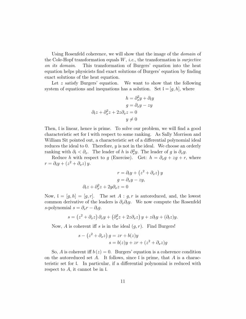
Using Rosenfeld coherence, we will show that the image of the domain ofthe Cole-Hopf transformation equalsW , i.e., the transformation is surjectiveon its domain. This transformation of Burgers’ equation into the heatequation helps physicists find exact solutions of Burgers’ equation by findingexact solutions of the heat equation.Let z satisfy Burgers’ equation. We want to show that the following

system of equations and inequations has a solution. Set l = [g, h], where

h = ∂2xy + ∂ty

g = ∂xy − zy∂tz + ∂2xz + 2z∂xz = 0

y 6= 0Then, l is linear, hence is prime. To solve our problem, we will find a goodcharacteristic set for l with respect to some ranking. As Sally Morrison andWilliam Sit pointed out, a characteristic set of a differential polynomial idealreduces the ideal to 0. Therefore, y is not in the ideal. We choose an orderlyranking with ∂t < ∂x. The leader of h is ∂

2xy. The leader of g is ∂xy.

Reduce h with respect to g (Exercise). Get: h = ∂xg + zg + r, wherer = ∂ty + (z

2 + ∂xz) y.

r = ∂ty +¡z2 + ∂xz

¢y

g = ∂xy − zy,∂tz + ∂2xz + 2y∂xz = 0

Now, l = [g, h] = [g, r]. The set A : g, r is autoreduced, and, the lowestcommon derivative of the leaders is ∂x∂ty. We now compute the Rosenfelds-polynomial s = ∂xr − ∂tg.

s =¡z2 + ∂xz

¢∂xy +

¡∂2xz + 2z∂xz

¢y + z∂ty + (∂tz)y.

Now, A is coherent iff s is in the ideal (g, r). Find Burgers!

s− ¡z2 + ∂xz¢g = zr + b(z)y

s = b(z)y + zr + (z2 + ∂xz)g

So, A is coherent iff b (z) = 0. Burgers’ equation is a coherence conditionon the autoreduced set A. It follows, since l is prime, that A is a charac-teristic set for l. In particular, if a differential polynomial is reduced withrespect to A, it cannot be in l.

11

So, `∂x is a surjective map from its domain V \ {0}, the set of nonzerosolutions of the heat equation onto W , the solution set of Burgers’ equation.The fiber `∂−1(z), z ∈ W , is the set of solutions of the pair of differentialequations

∂xy

y= z

∂ty

y= −(z2 + ∂xz)

This pair of differential equations has a solution ⇐⇒ b (z) = 0. So, Burg-ers’equation is the integrability condition in the classical sense. The proofin differential algebraic geometry uses Rosenfeld coherence. Note that thefiber of `∂x is a ∂-variety that is finite-dimensional, of dimension 1. Eachfiber gives us a finite-dimensional ∂-subvariety of the infinite-dimensional∂-variety V (h).

2 Affine differential algebraic groups.

Definition 2.1. 1. Let G be a group. G is an affine ∂-group if, for somen, G is a Kolchin closed subset of An, and, the group multiplicationG×G→ G and inversion G→ G are morphisms of ∂-varieties. If mul-tiplication and inversion are defined over F, and, the identity element1 has coordinates in F, we call G a ∂-F-group.

2. Let G be a ∂-group. There is a unique component G0 containing 1,which is a normal ∂-subgroup whose cosets are the irreducible compo-nents of G. In particular, the components are mutually disjoint, and,of course, equal the connected components of G.

3. IfG and G are affine ∂-groups, a homomorphism f : G→ G of ∂-groupsis a group homomorphism, and, a ∂-variety morphism.

Remark 2.2. Every affine algebraic group is an affine ∂-group.

1. Let G be a ∂-group, and, let a ∈ G. An important homomorphism of∂-groups is the inner automorphism x 7−→ axa−1.

12

2. The additive group Gna of Un is a ∂-group. Let Li, i = 1, . . . , n ∈U [∂], the non-commutative ring of linear differential operators (non-commuting polynomials) in ∂1, . . . , ∂m. Let l be the surjective ∂-endomorphism of Gna with coordinate functions L1, . . . , Ln. Every∂-endomorphism of Gna is in this form.

Let f : G→ G be a ∂-group homomorphism. It is easy to see that ker fis a normal ∂-subgroup of G. The fact that imf is a subgroup of G followsfrom the Chevalley-Seidenberg Theorem. If G and G are ∂-F-groups, and,f is defined over F, then, ker f , and, im f are ∂-F-groups.

If f : G → G is a homomorphism, f (G0) is the identity component ofim f . So, the image of a connected ∂-group is connected.

Notation 2.3. If G is an affine ∂-F-group, the subgroup of points in G withcoordinates in a ∂-extension field G of F in U is denoted by G (G).

As we saw in Jerry Kovacic’s talks, GLn (U) is a Zariski open set inAn2 =Mn (U). We close it up by identifying it with the ∂-subgroup of An

2+1

defined by the equation z det y = 1, where y = (yij)i,j=1,...,n.is a matrix of

differential indeterminates. The coordinate ring of GLn (U) is U©(yij),

1det

ª.

When we give the defining equations of a ∂-subgroup of GLn (U), we willomit the equation z det y = 1, since it is universally satisfied. We denoteGL1 (U) by Gm.

Remark 2.4. Let R be the field of real numbers, and, U a differential closureof the quotient field F of the ring of real analytic functions on the unit circleS1. GLn (F) = GLn (R) ⊗R F can be conceptualized as the loop groupMap (S1, GLn (R)).

An affine ∂-group G is linear if there is an isomorphism from G into someGLn (U). Every affine algebraic group is linear.

Example 2.5. Let U be an ordinary differential field with derivation oper-ator ∂.

1. The only algebraic group structure on the affine plane A2 (over any al-gebraically closed field of characteristic 0) is the additive groupGa×Ga.The following are the ∂-group structures on A2 (up to isomorphism):

(u1, u2) (v1, v2) =

Ãu1 + v1, u2 + v2 +

Xi<j

u(i)1 v

(j)1

!

13

where u(i) = ∂iu. (The sumPi<j

u(i)1 v

(j)1 is a differential polynomial 2-

cocycle from Ga into Ga.) These groups are unipotent linear ∂-groups.The group is “unipotent” since it can be embedded in a group of uppertriangular matrices with 10s on the diagonal.

For example, the group (u1, u2) (v1, v2) =³u1 + v1, u2 + v2 + u1v1 + u1v

(2)1

´is isomorphic to a ∂-group of 4× 4 unipotent matrices:

1 u1 u´1 u20 1 0 u10 0 1 u

(2)1

0 0 0 1

If U is an ordinary differential field, the logicians Pillay and Kowalskiproved that every ∂-group structure with underlying variety An is aunipotent linear group.

2. (Cassidy-Kovacic) Let t ∈ U, transcendental over Q, with ∂t = 1. SetG equal to the Kolchin closed subset of A2, defined by the differentialequations:

y2 (y1 − 1)2 = t2¡y31 + ay1y

22 + by

32

¢∂y1 =

1

t

¡y21 − y1

¢y1∂y2 − y2∂y1 = 0.

where a, b ∈ Q, b 6= 0, 4a3 + 27b2 6= 0. G is a connected commutative∂-Q (t)-group. 0 = (0, 0). Note that y2 = 0 implies y1 = 0, and, that2y1 − 1 never vanishes on G (Exercise). − (y1, y2) =

³y1

2y1−1 ,y2

2y1−1´.

Coordinatize G×G by (y1, y2) , (z1, z2). On the open set y1y2(y1z2 −y2z1) 6= 0, the addition law is given by (v1, v2), where

v1 =1

t2

µy1z2 − z1y2 + y2 − z2

y1z2 − y2z1

¶2− y1z2 + y2z1

y2z2.

v2 = − 1t3

µy1z2 − y2z1 + y2 − z2

y1z2 − y2z1

¶3+

+1

t.

µµy1z2 − y2z1 + y2 − z2

y1z2 − y2z1

¶µy1z2 + y2z1y2z2

¶−µ

z1 − y1y1z2 − y2z1

¶¶

14

Perhaps you realized that the affine ∂-Q (t)-group G is an embeddingin the affine U-plane of the ∂-subgroup E (K) consisting of the constantpoints of the elliptic curve in the projective U-plane with affine equationy22 = y31 + ay1 + b The embedding is a rational isomorphism defined overQ (t). G is not linear. G has no non-trivial linear representations. Theproof mainly consists in counting the number of points of order dividing n.The group of example 1 is not finite-dimensional if the transcendence

degree of U over Q is infinite. The group of example 2 is finite-dimensional.

Problem 2.6. 1. Characterize all affine non-linear differential algebraicgroups

2. When U is an ordinary differentially closed differential field, the lo-gicians Hrushovski, Sokolovich, and Pong, have shown that all finite-dimensional ∂-groups can be embedded in the affine U-line. Charac-terize all affine differential algebraic groups with no non-trivial linearrepresentations. Are they all commutative? Must they be finite-dimensional? Are they all obtained by affine ∂-embeddings of abelianvarieties?

3 Linear differential algebraic groups.

For ease of exposition, we reluctantly assume that U is an ordinary differentialfield with derivation operator ∂, and field K of constants. As usual, we oftendenote ∂y by y0, ∂2y by y00,....Everything in the following discussion has aparallel in the partial case.Let G be an affine ∂-group, with coordinate ring U {G} = R, and, ring of

everywhere defined differential rational functions bR. Let a ∈ G. We definea ∂-automorphism over U of bR by

(fa)(b) = f(ba), f ∈ bR, b ∈ G.If G = GLn (U), then, (yij)a =

Pnk=1 yikakj. The map ρ : G → Aut∂bR is

an injective homomorphism of groups, called the regular representation of G.If G is a subgroup of GLn (U), then, for all a ∈ G, for all f ∈ R, fa is in R.In this case, we refer to the restriction of the regular representation to R asthe regular representation of G.

15

Theorem 3.1. Let G be a linear ∂-group, and, let N be a normal ∂-subgroup.There exists a linear ∂-group G0, and, a surjective homomorphism q : G →G0, with kernel N such that if H is a linear ∂-group, and, f : G → H is ahomomorphism whose kernel contains N , there is a homomorphism g : G0 →H such that g ◦ q = f .G0 is called the quotient group of G by N , and, is denoted by G/N .Let G be a ∂-subgroup of GLn (U), and, let H be a ∂-subgroup of G.

S = {f ∈ R : fa = f ∀h ∈ H} is a ∂-subalgebra over U of R called the ringof invariant differential polynomal functions of H.Recall: Not every differential polynomial ideal is finitely differentially

generated (J. F. Ritt). Boris Weisfeiler ingeniously adapted Ritt’s exampleto show that, in contrast to algebraic group theory, the ring of invariants inU {y} (under the regular representation of Gm) of the finite subgroup {±1} isnot finitely ∂-generated. If we replace U {y} by the coordinate ring U

ny, 1

y

o,

which is a Hopf algebra, this cannot happen..

Theorem 3.2. If G is a ∂-subgroup of GLn (U), and, N is a normal ∂-subgroup of G, the subring S ⊂ R of invariant differential polynomial func-tions of N is finitely ∂-generated.

Corollary 3.3. Let G = G/N . Then, the coordinate ring U {G } is iso-morphic over U to the ∂-algebra over U of invariants of N in U {G}.Problem 3.4. Prove that quotients of affine ∂-groups exist. Are they alsoaffine?

3.1 The differential algebraic subgroups of Gm.The only proper algebraic subgroup of Ga is {0}. If G is a ∂-subgroup,there exist linear differential operators L1, . . . , Lr ∈ U [∂] such that G =Tri=1 kerLi.The only proper algebraic subgroups of Gm are the groups G of nth roots

of unity. The defining equation of G is yn−1 = 0. f(y) = yn−1 is also thedefining differential polynomial invariant of G. The next theorem tells usthat all the ∂-subgroups of Gm are defined by a single differential polynomialinvariant in U {Gm (U)} = U

ny, 1

y

o= R.

16

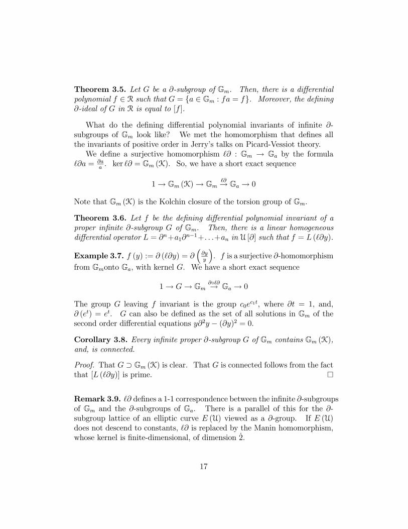
Theorem 3.5. Let G be a ∂-subgroup of Gm. Then, there is a differentialpolynomial f ∈ R such that G = {a ∈ Gm : fa = f}. Moreover, the defining∂-ideal of G in R is equal to [f ].

What do the defining differential polynomial invariants of infinite ∂-subgroups of Gm look like? We met the homomorphism that defines allthe invariants of positive order in Jerry’s talks on Picard-Vessiot theory.We define a surjective homomorphism `∂ : Gm → Ga by the formula

`∂a = ∂aa. ker `∂ = Gm (K). So, we have a short exact sequence

1→ Gm (K)→ Gm`∂→ Ga → 0

Note that Gm (K) is the Kolchin closure of the torsion group of Gm.

Theorem 3.6. Let f be the defining differential polynomial invariant of aproper infinite ∂-subgroup G of Gm. Then, there is a linear homogeneousdifferential operator L = ∂n+a1∂

n−1+. . .+an in U [∂] such that f = L (`∂y).

Example 3.7. f (y) := ∂ (`∂y) = ∂³∂yy

´. f is a surjective ∂-homomorphism

from Gmonto Ga, with kernel G. We have a short exact sequence

1→ G→ Gm∂◦`∂→ Ga → 0

The group G leaving f invariant is the group c0ec1t, where ∂t = 1, and,

∂ (et) = et. G can also be defined as the set of all solutions in Gm of thesecond order differential equations y∂2y − (∂y)2 = 0.Corollary 3.8. Every infinite proper ∂-subgroup G of Gm contains Gm (K),and, is connected.

Proof. That G ⊃ Gm (K) is clear. That G is connected follows from the factthat [L (`∂y)] is prime.

Remark 3.9. `∂ defines a 1-1 correspondence between the infinite ∂-subgroupsof Gm and the ∂-subgroups of Ga. There is a parallel of this for the ∂-subgroup lattice of an elliptic curve E (U) viewed as a ∂-group. If E (U)does not descend to constants, `∂ is replaced by the Manin homomorphism,whose kernel is finite-dimensional, of dimension 2.

17

3.2 Simple differential algebraic groups.

Definition 3.10. 1. Let G be an affine ∂-group, and V a ∂-variety. Anaction ofG on V is a triple (G, V, f), where f is a morphismG×V → V ,sending (z, x) to zx = f (z, x), such that

1x = x

z1 (z2x) = (z1z2)x

z1, z2 ∈ G, x ∈ V .2. V is a homogeneous space forG if the action is transitive,i.e., for everyx,y ∈ V there is z ∈ G such that zx = y. A homogeneous space V is atorsor under G if there is a unique such z.

3. Let x ∈ V . The set of all z ∈ G such that zx = x is a ∂-subgroup ofG called the isotropy group of x.

Definition 3.11. An infinite algebraic group is simple if it is not commu-tative, and, every proper normal algebraic subgroup is finite. Similarly, a∂-group G is simple if it is not commutative, and, every proper normal ∂-subgroup is finite. In particular, G is connected.

Theorem 3.12. (Pillay) Every simple ∂-group is linear.

Definition 3.13. A Chevalley group is a simple algebraic group that is de-fined over Q.

Theorem 3.14. (The classification of the simple ∂-groups) Let G be asimple ∂-group. There exists a simple Chevalley group H such that G isisomorphic to H (U) or to H (K), the group of matrices in G with entries inK.

Corollary 3.15. Every simple ∂-group G can be realized as a simple Cheval-ley group H (U) or as a simple Chevalley group H (K).

For an arithmetic analogue that replaces the derivation ∂ with a nonlinearoperator on a p-adic ring, see Buium (1998).

18

3.2.1 The Zariski dense ∂-subgroups of SLn (U).

The first step in the proof of the classification theorem of the simple ∂-groups G entails embedding G in a simple Chevalley group G as a Zariskidense ∂-subgroup. Conversely, every Zariski dense ∂-subgroup of a simpleChevalley group is simple. To illustrate the second step, which describes theproper Zariski dense ∂-subgroups of a simple Chevalley group H, we takeH = SLn (U).

Definition 3.16. Let k be a field. A vector space g over k is a Lie algebraif there is a bilinear map m : g× g→ g, sending (a, b) to [a, b] such that:

1. [a, a] = 0. antisymmetry =⇒ [b, a] = − [a, b]2. [a, [b, c]] + [b, [c, a] + [c, [a, b]] = 0 Jacobi identity

The vector spaceMn (U) is a Lie algebra over U. If A and B are matrices,[A,B] = AB − BA. It is denoted by g`n (U). It is the Lie algebra ofmatrices of GLn (U). The Lie subalgebra that interests us is s`n (U) ={A ∈ s`n (U) : tr(A) = 0}. It is the Lie algebra of matrices of SLn (U).SLn (U) acts on s`n (U) by the adjoint action: Ad(Z) : A 7−→ ZAZ−1, Z ∈

SLn (U),A ∈ s`n (U). The adjoint action maps SLn (U) into the automor-phism group of the Lie algebra s`n (U). Its kernel is the center {$ 1n : ω

n = 1}.In differential algebraic geometry, as well as in Picard-Vessiot theory,

there is another action of SLn (U) on s`n (U), called the gauge action. It isbuilt from the logarithmic derivative morphism.`∂ : GLn (U)→ g`n (U):

`∂(Z) = ∂Z Z−1.

If Z = (zij), ∂Z = (∂zij). Now, tr (`∂ (Z)) = `∂ (det(Z)) (Exercise). So,`∂ maps SLn(U) into s`n (U). One can show that it is surjective since U isdifferentially closed.Although `∂ is a morphism of ∂-varieties, it is not a homomorphism of

groups.`∂ (Z1Z2) = `∂ (Z1) + Z1`∂ (Z2)Z

−11

`∂ is what we call a crossed homomorphism (1-cocycle), with respect to theadjoint action. Thus, it has a kernel, which is SLn (K).`∂ gives rise to the gauge action of the ∂-group SLn (U) on its Lie algebra

s`n (U).A 7−→ ZAZ−1 + `∂ (Z) = `∂ (Z) + ZAZ−1.

19

Since U is differentially closed, s`n (U) is a homogeneous space for the speciallinear group under this action. If we restrict the actors and actees to anarbitrary base field F, the action may no longer be transitive. The orbitsthen play an important role in Picard-Vessiot theory.

Remark 3.17. Let V be a finite-dimensional vector space. The affine groupof V is the group of all transformations v 7−→ T (v)+w, where T is linear andw ∈ V . The gauge action maps SLn (U) into the affine group of the vectorspace s`n (U) over U. The affine group is a linear group, and, so, as in thecase of the adjoint action, the gauge action gives us a linear representationof SLn (U)— this time as a differential algebraic group, rather than as analgebraic group. What is the kernel of this representation? Setting A = 0,we see that Z ∈ SLn (K). But, then, Z is in ker Ad, which is the center ofSLn (U). So, the adjoint action and the gauge action have the same kernel.

Let A ∈ s`n (U). The isotropy group G of A in SLn (U) under the gaugeaction is defined by the differential equations

detY = 1

A = Y AY −1 + ∂Y Y −1

The second equation is a matrix equation, which is usually written ∂Y =AY − Y A = [A, Y ], and, is called a Lax equation. Lax equations play animportant part in the isomonodromy approach to Painleve theory. Theequation gives rise to n2 linear homogeneous differential polynomial equa-tions. It is easy to see that the isotropy group of A is a proper Zariski dense∂-subgroup of SLn(U).The main step in the classification theorem is the following theorem.

Recall that a ∂-F-subgroup of GLn(U) is a ∂-subgroup that is defined overF.

Theorem 3.18. Let G be a proper Zariski dense ∂-F-subgroup of SLn (U)Then, there is a matrix A ∈ s`n (F) such that G is the isotropy group of Aunder the gauge action.

Corollary 3.19. Let G be a proper Zariski dense ∂-F-subgroup of SLn (U).Then, there is a Picard-Vessiot extension G of F and a matrix T ∈ s`n (G)such that T−1GT = SLn (K).

20

Proof. Since the logarithmic derivative morphism is surjective, there is amatrix T ∈ SLn (U) such that `∂(T ) = A. Indeed, we can find such amatrix T generating a Picard-Vessiot extension of F. Let Z ∈ G. We willnot prove here that we can find a matrix T that is Picard-Vessiot over F.

`∂¡T−1ZT

¢= `∂

¡T−1

¢+ T−1`∂ (ZT )T

= T−1(−`∂ (T ) + `∂ (Z) + Z`∂ (T )Z−1)T= T−1

¡−A+ `∂ (Z) + TAT−1¢= 0.

Therefore, T−1ZT ∈ SLn (K). Similarly, one can show that TSLn (K)T−1is the isotropy group of A = `∂ (T ) under the gauge action of SLn (U) ons`n (U).

4 The Action of SL2 on Riccati varieties.

This is the story of configurations of 4 points on the projective line. It isa plain and casual narrative, intending to show the connection between thegauge action of differential equations theory, and, projective linear transfor-mations, and, between circles in the extended complex plane and Riccativarieties.You may ask what 4 points on the projective line have to do with simple

differential algebraic groups. Have patience, and you will find out.For an engrossing, clearly written, modern treatment of the configuration

space of 4 points on the complex projective plane, see Masaaki Yoshida,Hypergeometric Functions, My Love, 1997. Yoshida dedicates his book tohis cats, and, his “dog, Fuku, who came to my house from nowhere to livewith me.”Recall the Riccati equation from the lectures on Picard-Vessiot theory

R (a0, a1, a2) : y0 = a0 + a1y + a2y2, (a0, a1, a2) ∈ U3,

A ∂-subvariety of A1(U) defined by a Riccati equation is called a Riccativariety. Note that there is a 1-1 correspondence between the set of Riccatiequations and U3.The differential algebraic geometry of a Riccati variety is interesting. We

embed it in the projective line P1 (U).

21

Let k be a field. P1 (k) is the set of equivalence classes of pairs

(u1, u2) ∈ A2 (k) (u1, u2) 6= 0,under the equivalence relation

(u1, u2) ∼ (λu1,λu2) λ ∈ k,λ 6= 0.The class of (u1, u2) is denoted by [u1, u2].A polynomial P ∈ k [y1, y2] is homogeneous if there is a positive integer

d such that for all λ ∈ k, P (λy1,λy2) = λdP (y1, y2). A subset of P1(k) isZariski closed if it is the set of zeros of a finite set of homogeneous polynomialsin k [y1, y2].Similarly, a differential polynomial P ∈ U{y1, y2} is ∂-homogeneous if

there is a positive integer d such that for all λ ∈ U, P (λy1,λy2) = λdP (y1, y2).Clearly, P must be a homogeneous polynomial. A subset of P1(U) is Kolchinclosed if it is the set of zeros of a finite set of ∂-homogeneous differentialpolynomials in U{y1, y2}.We refer to the equivalence classes [u1, u2] as points on the projective line.P1(k) is covered by 2 affine open patches: y2 6= 0, and, y1 6= 0. We

are interested only in the patch O : y2 6= 0. The point “at infinity” (not inO) is [1, 0], which is in the other affine open patch. If [u1, u2] ∈ O, then,[u1, u2] = [u, 1], where u =

u1u2. So, we identify O with A1 (k) by the map

[u1, u2] 7−→ u.We identify P1(k) with the extended k-line k ∪ {∞} = O ∪ {[1, 0]}.Set k = U. K = U∂. The Kolchin closed set P1 (K) = {[c1, c2] : c1, c2 ∈ K}

is defined by the differential polynomial

y2y01 − y02y1.

For the action of SL2 on the set of Riccati equations, see “Integrability ofthe Riccati equation from a group theoretical viewpoint,” Jose F. Carinena,Artur Ramos, arXiv.org.math-ph19810005.If V is the Riccati variety defined by R (a0, a1, a2), we embed it in the

projective line as follows:We homogenize R (a0, a1, a2): Set y =

y1y2.µ

y1y2

¶0= a0 + a1

y1y2+ a2

µy1y2

¶2.

22

Multiply through by y22. The homogenization is:

y01y2 − y1y02 = a0y22 + a1y1y2 + a2y21.

Lemma 4.1. The affine Riccati variety equals its projective closure if andonly if a2 6= 0.Proof. The point [1, 0] at infinity satisfies the homogenization of the Riccatiequation iff a2 = 0.

Let k be any field of characteristic zero. PGL2(k) is the group consistingof all projective linear transformations :

τ(u) =αu+ β

γu+ δM =

µα βγ δ

¶∈ GL2 (k) .

Note that the transformation may send u ∈ O “to ∞.” This happens whenu = − δ

γ. τ is invertible, with inverse represented by M−1.

The map M 7−→ τ , defined as above, is a surjective homomorphism from

GL2(k) onto PGL2 (k)with kernel the center

µα 00 α

¶,α ∈ Gm(k). It

defines on PGL2(k) the structure of algebraic group. If k = U, it hasdefined on it the canonical structure of differential algebraic group. Both ofthese structures are inherited from the general linear group.

Suppose k is algebraically closed. Let M =

µα βγ δ

¶∈ GL2 (k).

Then, 1√detM

M =

Ãα√detM

β√detM

γ√detM

δ√detM

!∈ SL2(k) and has the same image

in PGL2 (k). So, PGL2 (k) = PSL2 (k).

Remark 4.2. 1. Given a projective linear transformation

τ(u) =αu+ β

γu+ δ,

represented by the matrix M =

µα βγ δ

¶. Then, τ (∞) = ∞ if and

only if

µαγ

¶=M

µ10

¶=

µα0

¶.

23

So, the projective linear transformations fixing ∞ are the affine trans-formations τ (u) = εu+ η, ε ∈ Gm(k), η ∈ Ga (k).

J (u) = 1u, represented by M =

·0 11 0

¸, interchanges 0 and ∞.

2. Let k = C, the field of complex numbers. Projective linear transfor-mations of C ∪ ∞ are often called Mobius transformations, and, theextended C-line is called the extended complex plane.When k is algebraically closed, PGL2(k) is connected. However, thisneed not be the case if k is not algebraically closed.

PGL2 (R) is not connected. Multiply M ∈ GL2(R) by 1√|detM | .

Then, det

µ1√

|detM |M¶= ±1, and, the images of M and 1√

|detM |M in

PGL2 (R) are the same. We may assume, therefore, that detM = ±1.

The matrix

µ0 11 0

¶has determinant −1, and, its square is the iden-

tity matrix. Therefore, if detM = −1,M =

µ0 11 0

¶µµ0 11 0

¶M

¶.

Thus, PGL2(R) has two components: PSL2(R) and the projectivetransformations associated with matrices in GL2(R) with determinant−1.PGL2 (R) = PSL2(R)∪ J ·PSL2(R), where J (u) = 1

u, represented byµ

0 11 0

¶.

Lemma 4.3. Given a triple (u1, u2, u3) of distinct points in P1(k), there is aunique projective linear transformation λ mapping (u1, u2, u3) onto (0, 1,∞).It is given by the formula:

λ (u) =(u− u1)(u2 − u3)(u1 − u2) (u3 − u)

Note that the determinant of the representing matrix is

(u1 − u2) (u2 − u3) (u3 − u1).

So, it is invertible.

24

Definition 4.4. λ (u) is called the cross-ratio (anharmonic ratio) of thequadruple (u, u1, u2, u3).

Remark 4.5. The definition of cross-ratio is dependent on the order ofthe points u, u1, u2, u3. There are 6 values of the cross-ratio under the 24permutations of u, u1, u2, u3 :

λ, 1− λ,1

λ,

λ

λ− 1 ,1

1− λ,λ− 1λ

.

Corollary 4.6. Given two triples (u1, u2, u3), (v1, v2, v3) of distinct points inP1(k), there is a unique projective linear transformation τ mapping (u1, u2, u3)onto (v1, v2, v3).

Corollary 4.7. Let (u, u1, u2, u3) and (v, v1, v2, v3)be quadruples of points inP1 (k) such that u1, u2, u3 are distinct, as are v1, v2, v3. Then, there is aprojective linear transformation τ mapping (u, u1, u2, u3) onto (v, v1, v2, v3) ifand only if their cross-ratios are equal.

Proof. Suppose the transformation τ maps (u, u1, u2, u3) onto (v, v1, v2, v3).Let υ be the unique transformation mapping (v1, v2, v3) onto(0, 1,∞). Then,υ (v) = λ (v). υτ (u, u1, u2, u3) = (λ (u) , 0, 1,∞) = υ (v, v1, v2, v3) = (λ (v) , 0, 1,∞).So, their cross-ratios are equal.Conversely, suppose λ (u) = λ (v) . Then, there exists υ, τ such that

υ (u, u1, u2, u3) = (λ, 0, 1,∞) = τ (v, v1, v2, v3). Therefore, υ−1τ (u, u1, u2, u3) =

(v, v1, v2, v3).

Corollary 4.8. Cross-ratio is an invariant of the projective linear group.

A circle (which may be a straight line) in the extended complex planeC ∪ {∞} is uniquely determined by a triple (u1, u2, u3) of points on thecircle. The unique circle passing through (0, 1,∞) is R ∪ {∞}.All affine transformations τ (u) = αu + β, α ∈ Gm (C) , β ∈ Ga (C),

transform circles into circles, since multiplication by α rotates and perhapsstretches or contracts the circle, and, translation moves the circle to anothercenter. The transformation u 7−→ 1

ureflects the circle in the real axis and

perhaps stretches or contracts. So,

Lemma 4.9. Every projective linear transformation maps a circle onto acircle.

25

We now show that PSL2 (C) acts transitively on the set of circles in theextended complex plane.

Proposition 4.10. Let C and C 0 be circles in the extended complex plane.Then, there is a projective linear transformation τ mapping C onto C 0.

Proof. Let (u1, u2, u3) be a triple of distinct points on C, and, (v1, v2, v3)be a triple of distinct points on C 0. Let τ be the unique transformationmapping (u1, u2, u3) onto (v1, v2, v3). τ (C) is a circle containing (v1, v2, v3).Therefore, τ (C) = C 0.

Proposition 4.11. Let C be the circle in the extended complex plane throughthree distinct points u1, u2, u3. Then,C is the set of all points u ∈ P1(C) suchthat the cross-ratio

λ (u) =(u− u1)(u2 − u3)(u1 − u2) (u3 − u)

of (u, u1, u2, u3) is in P1 (R) = R ∪ {∞}.Proof. Let τ be the transformation that carries (u1, u2, u3) to (0, 1,∞). Then,τ (C) = P1 (R).

Definition 4.12. Let k be a field, and let S ⊂ P1(k). The set of allprojective linear transformations τ mapping S into S (restricting to self-maps of S) is a subgroup of PGL2 (k), called the stabilizer of S, and isdenoted by G (S).

Theorem 4.13. Let C be a circle in P1 (C). The stabilizer G(C) is conjugateto PGL2 (R).

Proof. There exists a projective linear transformation τ such that τ (C) =P1 (R). The stabilizer G (P1 (R)) = PGL2 (R). Therefore, it is not hard tosee that τG(C)τ−1 = G (P1 (R)).

Let τ be in PGL2 (R). Since τ is a homeomorphism (of the Riemannsphere), it maps each of the disks bounded by C onto a disk bounded byP1 (R), namely, onto the upper half plane U or onto the lower half planeL. The stabilizer G (U) of the upper half plane is PSL2 (R), and, since theinversion map J maps U onto L, if the matrix representing τ has determi-nant −1, τ interchanges the upper and lower half planes. Let S ∈ SL2(R)represent a transformation σ ∈ PSL2 (R), and, let T ∈ SL2(C) represent

26

τ ∈ PGL2(C). Then T−1ST represents τ−1στ . det(T−1ST ) = 1. So,T−1ST ∈ SL2 (C). So, we have:

Theorem 4.14. The stabilizer G in SL2(C) of a circle C in the extendedcomplex plane under the action by PSL2 (C) is conjugate in SL2(C) toSL2(R). G also stabilizes each disk bounded by the circle.

4.1 The action of SL2 (U) on the set of Riccati varieties

We identify the set of Riccati equations R (a0, a1, a2) : y0 = a0 + a1y + a2y2

with U3 : R (a0, a1, a2) 7−→ a0a1a2

. SL2 (U) acts on the set of Riccati

equations as follows:

Let Z =

µα βγ δ

¶,αδ − βγ = 1. Map

a0a1a2

to

b0b1b2

, where b0b1b2

=

α2 −αβ β2

−2αγ αδ + βγ −2βδγ2 −γδ δ2

a0a1a2

+ αβ0 − α0β2 (α0δ − β0γ)γδ0 − γ0δ

.This action transforms R (a0, a1, a2) into R (b0, b1, b2). The inverse transfor-mation is a0

a1a2

=

δ2 βδ β2

2δγ αδ + βγ 2αβγ2 αγ α2

b0b1b2

+ βδ0 − β0δ2 (αδ0 − β0γ)αγ0 − α0γ

.Lemma 4.15. Let V be the Riccati variety defined by R (a0, a1, a2). Let

Z =

µα βγ δ

¶,αδ − βγ = 1.. The projective linear transformation

τ (u) =αu+ β

γu+ δ

transforms V into the Riccati varietyW defined by R (b0, b1, b2), where R (b0, b1, b2)is the transform by Z of Riccati equation R (a0, a1, a2).

27

Proof. A tedious but straightforward computation shows that τ(V ) ⊂ W .τ−1 then maps W into V . So, τ restricts to an isomorphism of V ontoW .

Corollary 4.16. Every projective linear transformation in PSL2 (U) mapsa Riccati variety onto a Riccati variety.

Corollary 4.17. Let (u1, u2, u3) be a triple of distinct points in P1 (U).There is a unique Riccati variety containing u1, u2, u3.

Proof. Let τ−1(u) = αu+βγu+δ

be the unique transformation mapping (u1, u2, u3)

onto (0, 1,∞). Then, τ maps the Riccati variety P1 (K) onto a Riccati varietyV containing u1, u2, u3. IfW is a Riccati variety containing the three points,then, τ (P1 (K)) =W = V .

Corollary 4.18. Let V be the Riccati variety in the extended U-line throughthree distinct points u1, u2, u3. Then, V is the set of all points u ∈ P1(U)such that the cross-ratio

λ (u) =(u− u1)(u2 − u3)(u1 − u2) (u3 − u)

of u, u1, u2, u3 is in P1(K).

Corollary 4.19. Let V be the Riccati variety in the extended U-line throughthree distinct points u1, u2, u3. Then, V is the set of all points u ∈ P1(U)such that

u =c (u1 − u2) + u1(u2 − u3)c(u1 − u2) + (u2 − u3) , c ∈ P

1(K).

This formula, called a superposition principle, gives us the transformationτ . We have represented τ by a matrix in GL2(U). det τ = (u1 − u2)(u2 −u3)(u3−u1). Notice that the elements of the Riccati variety depend rationallyon one “arbitrary constant.” In differential equations theory, the Riccatiequation is a differential equation with no movable singularities (movablepoles are allowed).What do the stabilizers of Riccati varieties look like?

Theorem 4.20. The stabilizer G(V ) of a Riccati variety in PSL2 (U) isconjugate to PSL2 (K).

Proof. Let τ be a projective linear transformation mapping V onto P1 (K).The stabilizer of P1 (K) is PSL2 (K). τG(V )τ−1 = PSL2(K).

28

4.2 The gauge action revisited

Recall that the gauge action of SL2 (U) on its Lie algebra sl2(U) is definedby the formula:

A 7−→ ZAZ−1 + ∂Z Z−1 A ∈ sl2(U), Z ∈ SL2(U).

The inverse of the gauge transformation by Z is

A 7−→ Z−1AZ − Z−1∂Z.

We now describe this affine transformation of sl2 (U) explicitly. Wechoose the following basis of sl2 (U):

E0 =

µ0 10 0

¶, E1 =

1

2

µ1 00 −1

¶, E2 =

µ0 0−1 0

¶.

Write A = a0E0 + a1E1 + a2E2 Then,

ZAZ−1 + ∂Z Z−1 = b0E0 + b1E1 + b2E2,

where b0b1b2

=

α2 −αβ β2

−2αγ αδ + βγ −2βδγ2 −γδ δ2

a0a1a2

+ αβ0 − α0β2 (α0δ − β0γ)γδ0 − γ0δ

.Theinverse is

a0a1a2

=

δ2 βδ β2

2δγ αδ + βγ 2αβγ2 αγ α2

b0b1b2

+ βδ0 − β0δ2 (αδ0 − β0γ)αγ0 − α0γ

.Note that the gauge action of SL2 (U) on sl2 (U) is the same as the action,

described in section 4.1, of SL2 (U) on the set of Riccati equations.

29

Proposition 4.21. Let G be a proper Zariski dense ∂-subgroup of SL2 (U).There exists a projective Riccati variety V such that V is a homogeneous spacefor G under the action of G on P1 (U) by projective linear transformations.G is the isotropy group under the gauge action of the matrix A representingthe defining equation of V .

Proof. G is the isotropy group under the gauge action of a matrix A =a0E0+a1E1+a2E3. The matrix A represents a Riccati equationR (a0, a1, a2).We set V equal to the projective variety defined by the Riccati equationR (a0, a1, a2). G fixes R (a0, a1, a2), since it fixes A under the gauge action.Therefore, the image G0 of G in the projective special linear group stabilizesV . Let τ be the unique transformation such that τ (V ) = P1 (K). Let uand v be in V . Let c = τ (u), and, d = τ (v). PSL2 (K) acts transitivelyon P1 (K). So, there is a transformation σ ∈ PSL2 (K), with σ (c) = d.Therefore, τ−1 ◦ σ ◦ τ maps u to v, and, is in G(V ).So, we know that the stabilizers of Riccati varieties in the projective

special linear group PSL2 (U)are precisely the images of simple ∂-groups thatcan be embedded in SL2(U) as proper subgroups. Note that if we know oneelement u0 in a Riccati variety V then we can describe every element u in Vas follows:

u =αu0 + β

γu0 + δ,

where Z =

µα βγ δ

¶is in the isotropy group in SL2(U) of the matrix A

∈ sl2(U) under the gauge action.For the saga of circles in the extended complex plane and their stabi-

lizers, see Hans Schwerdtfeger, Geometry of Complex Numbers, 1962, and,Daniel Pedoe, Circles: A Mathematical Point of View, both republished byDover Publications in 1979. An excellent discussion of Mobius transforma-tions, cross-ratio, and, circles, from the point of view of complex functiontheory, is Gareth A. Jones, and David Singerman, Complex Functions: AnAlgebraic and Geometric Viewpoint, 1987. For a contrasting discussion ofRiccati varieties from the viewpoint of differential equations theory, see EarlD. Rainville, Intermediate Differential Equations, 1943.

30