Erhardt, Erik Barry, Masters Thesis - Worcester Polytechnic Institute

BAYESIAN SIMULTANEOUS INTERVALS FOR SMALL AREAS:

AN APPLICATION TO MAPPING MORTALITY RATES

IN U.S. HEALTH SERVICE AREAS

A Thesis

Submitted to the Faculty

of

Worcester Polytechnic Institute

by

Erik Barry Erhardt

In Partial Fulfillment of the

Requirements for the

Degree of Master of Science

in

Applied Statistics

December 2003

APPROVED:

Balgobin Nandram, Major Professor

Bogdan M. Vernescu, Department Head

ii

To my family,

who made everything I am possible

(regardless of how improbable).

iii

ACKNOWLEDGMENTS

Dr. Balgobin Nandram, my thesis advisor, for his support, guidance, advice and

conversation. A truely remarkable man and statistician.

Dr. Jai W. Choi for serving as an external examiner at my presentation November

24, 2003.

Dr. Jai W. Choi, Jimmie Givens and Dr. Paul Doug Williams for their assis-

tance during my internship at DHHS/CDC/NCHS/ORM (Office of Research and

Methodology at the National Center for Health Statistics of the Centers for Disease

Control of the Department for Health and Human Services). Thanks to Linda Pickle

for providing the data.

Mark Senn, in charge of the Purdue LATEX Project, for providing a beautiful and

functional LATEX template.

I presented talks on this thesis on August 15, 2003, at the National Center for

Health Statistics, Hyattsville, Maryland, and on Novemeber 24, 2003, at the Depart-

ment of Mathematical Sciences, Worcester Polytechnic Institute. I am grateful for

their comments, also.

iv

TABLE OF CONTENTS

Page

LIST OF TABLES . . . . . . . . . . . . . . . . . . . . . . . . . . . . . . . . . viii

LIST OF FIGURES . . . . . . . . . . . . . . . . . . . . . . . . . . . . . . . . x

ABBREVIATIONS . . . . . . . . . . . . . . . . . . . . . . . . . . . . . . . . . xiii

ABSTRACT . . . . . . . . . . . . . . . . . . . . . . . . . . . . . . . . . . . . xiv

1 Introduction . . . . . . . . . . . . . . . . . . . . . . . . . . . . . . . . . . . 1

1.1 Choropleth Maps . . . . . . . . . . . . . . . . . . . . . . . . . . . . . 1

1.2 Mapping Small Area Mortality . . . . . . . . . . . . . . . . . . . . . . 3

1.3 The 1996 Atlas . . . . . . . . . . . . . . . . . . . . . . . . . . . . . . 4

1.4 Models and Methods . . . . . . . . . . . . . . . . . . . . . . . . . . . 5

1.4.1 Rate Estimation . . . . . . . . . . . . . . . . . . . . . . . . . 5

1.4.2 Simultaneous Inference . . . . . . . . . . . . . . . . . . . . . . 7

1.5 Source of Data . . . . . . . . . . . . . . . . . . . . . . . . . . . . . . 10

1.5.1 Chronic Obstructive Pulmonary Disease (COPD) . . . . . . . 12

1.6 Bayesian Method . . . . . . . . . . . . . . . . . . . . . . . . . . . . . 13

1.7 Thesis Overview . . . . . . . . . . . . . . . . . . . . . . . . . . . . . . 14

2 Simultaneous Interval Estimation . . . . . . . . . . . . . . . . . . . . . . . 15

2.1 Review of Credible Intervals . . . . . . . . . . . . . . . . . . . . . . . 16

2.1.1 Credible Intervals (CI) . . . . . . . . . . . . . . . . . . . . . . 16

2.1.2 Highest Posterior Density (HPD) Intervals . . . . . . . . . . . 17

2.2 Simultaneous Intervals . . . . . . . . . . . . . . . . . . . . . . . . . . 23

2.2.1 Boole’s inequality . . . . . . . . . . . . . . . . . . . . . . . . . 23

2.3 Methods for constructing simultaneous 100(1− α)% intervals . . . . . 24

2.3.1 Simultaneous interval visualization example . . . . . . . . . . 26

2.4 Single-γ Method Simultaneous 100(1− α)% interval . . . . . . . . . . 29

v

Page

2.4.1 Single-γ Method Computations . . . . . . . . . . . . . . . . . 29

2.5 Double-γ Method Simultaneous 100(1− α)% interval . . . . . . . . . 31

2.5.1 Double-γ Method Computations . . . . . . . . . . . . . . . . . 31

2.6 Equal Ordinate condition optimization criterion . . . . . . . . . . . . 32

2.6.1 Maximum Relative Difference Criterion . . . . . . . . . . . . . 32

2.6.2 Average Relative Difference Criterion . . . . . . . . . . . . . . 32

2.6.3 Average Absolute Difference Criterion . . . . . . . . . . . . . 33

3 Simultaneous Intervals for a Hierarchical Poisson Model . . . . . . . . . . . 35

3.1 The Poisson-Gamma Hierarchical Regression Model . . . . . . . . . . 35

3.2 Computation using Markov chain Monte Carlo . . . . . . . . . . . . . 42

3.2.1 Metropolis-Hastings sampler . . . . . . . . . . . . . . . . . . . 42

3.2.2 Sampling . . . . . . . . . . . . . . . . . . . . . . . . . . . . . 45

3.2.3 Sampling Assessment . . . . . . . . . . . . . . . . . . . . . . . 46

3.3 Construction of the posterior interval maps . . . . . . . . . . . . . . . 49

3.3.1 Constructing the Mean Map . . . . . . . . . . . . . . . . . . . 50

3.3.2 Constructing the Credible Interval Map . . . . . . . . . . . . . 51

3.3.3 Constructing the HPD Interval Map . . . . . . . . . . . . . . 52

3.3.4 Constructing the Simultaneous Interval Map . . . . . . . . . . 54

3.3.5 Single-γ Method . . . . . . . . . . . . . . . . . . . . . . . . . 54

3.3.6 Double-γ Method . . . . . . . . . . . . . . . . . . . . . . . . . 55

3.3.7 Equal Ordinate condition optimization criterion . . . . . . . . 55

3.3.8 Maximum Relative Difference Criterion . . . . . . . . . . . . . 55

3.3.9 Average Relative Difference Criterion . . . . . . . . . . . . . . 56

3.3.10 Average Absolute Difference Criterion . . . . . . . . . . . . . 56

4 Maps and Assessment . . . . . . . . . . . . . . . . . . . . . . . . . . . . . . 59

4.1 Mean Legend Choropleth Maps . . . . . . . . . . . . . . . . . . . . . 60

4.1.1 Mean Map . . . . . . . . . . . . . . . . . . . . . . . . . . . . . 62

4.1.2 Individual HSA Credible Interval Map . . . . . . . . . . . . . 64

vi

Page

4.1.3 Individual HSA HPD Interval Map . . . . . . . . . . . . . . . 66

4.1.4 Single-γ Method Simultaneous Interval Map . . . . . . . . . . 68

4.1.5 Single-γ Method Simultaneous Interval by Region Maps . . . . 71

4.2 Mean Legend Difference Maps and Tables . . . . . . . . . . . . . . . 84

4.3 Individual Legend Choropleth Maps . . . . . . . . . . . . . . . . . . . 87

4.3.1 Individual Legend Individual HSA Credible Interval Map . . . 88

4.3.2 Individual Legend Individual HSA HPD Interval Map . . . . . 90

4.3.3 Individual Legend Single-γ Method Simultaneous Interval Map 92

4.3.4 Individual Legend Single-γ Method Simultaneous Interval byRegion Maps . . . . . . . . . . . . . . . . . . . . . . . . . . . 94

4.4 Individual Legend Difference Maps and Tables . . . . . . . . . . . . . 107

4.5 Double-γ Method Simultaneous Interval . . . . . . . . . . . . . . . . 115

5 Conclusion . . . . . . . . . . . . . . . . . . . . . . . . . . . . . . . . . . . . 119

5.1 Accounting for map variation, epidemiological discussion . . . . . . . 119

5.2 Looking ahead . . . . . . . . . . . . . . . . . . . . . . . . . . . . . . . 120

LIST OF REFERENCES . . . . . . . . . . . . . . . . . . . . . . . . . . . . . 122

A Statistical Methodology . . . . . . . . . . . . . . . . . . . . . . . . . . . . . 129

A.1 Statistics . . . . . . . . . . . . . . . . . . . . . . . . . . . . . . . . . . 129

A.2 Bayesian Approach . . . . . . . . . . . . . . . . . . . . . . . . . . . . 130

A.2.1 Formal Bayesian Methodology . . . . . . . . . . . . . . . . . . 131

A.2.2 Predictive Distribution . . . . . . . . . . . . . . . . . . . . . . 134

A.2.3 Kernel Density Estimation . . . . . . . . . . . . . . . . . . . . 134

A.2.4 A Simple Example - N(µ, 1τ) . . . . . . . . . . . . . . . . . . . 135

A.2.5 Prior Elicitation and Non-informative Prior . . . . . . . . . . 136

A.3 Sampling from the Posterior Distribution . . . . . . . . . . . . . . . . 138

A.3.1 Stratified Sampling . . . . . . . . . . . . . . . . . . . . . . . . 138

A.3.2 Importance Sampling . . . . . . . . . . . . . . . . . . . . . . . 139

A.3.3 Monte Carlo Method . . . . . . . . . . . . . . . . . . . . . . . 139

vii

Page

A.3.4 Markov Chain . . . . . . . . . . . . . . . . . . . . . . . . . . . 141

A.3.5 Markov chain Monte Carlo . . . . . . . . . . . . . . . . . . . . 144

A.3.6 Metropolis-Hastings Algorithm . . . . . . . . . . . . . . . . . 145

A.3.7 Gibbs Sampling . . . . . . . . . . . . . . . . . . . . . . . . . . 147

A.4 Issues of Convergence . . . . . . . . . . . . . . . . . . . . . . . . . . . 147

B Appendices . . . . . . . . . . . . . . . . . . . . . . . . . . . . . . . . . . . 151

B.1 Specification of Hyper-parameter constants used in Section 3.1 . . . . 151

B.2 Poisson-Gamma model as a weighted average of prior mean and sam-ple mean . . . . . . . . . . . . . . . . . . . . . . . . . . . . . . . . . . 153

B.3 Besag Simultaneous Credible Regions Based on Order Statistics . . . 154

viii

LIST OF TABLES

Table Page

3.1 Regression Covariates (Risk Factors) . . . . . . . . . . . . . . . . . . 38

3.2 Quantile values from 10,000 iterates of the α and β0 through β4 modelparameters. . . . . . . . . . . . . . . . . . . . . . . . . . . . . . . . . 48

3.3 Sample summary for model parameters α and β0 through β4 from10,000 iterates. . . . . . . . . . . . . . . . . . . . . . . . . . . . . . . 48

4.1 Mean map minimum, maximum and quintiles and CI and HPD mapminimum lower and maximum upper values . . . . . . . . . . . . . . 62

4.2 Single-γ Method values for γ. . . . . . . . . . . . . . . . . . . . . . . 69

4.3 Simultaneous Probability Content by Region for different methods. . 69

4.4 Mean Legend Credible Interval difference between lower and upperbound maps. . . . . . . . . . . . . . . . . . . . . . . . . . . . . . . . . 86

4.5 Mean Legend HPD Interval difference between lower and upper boundmaps. . . . . . . . . . . . . . . . . . . . . . . . . . . . . . . . . . . . 86

4.6 Mean Legend Simultaneous Interval difference between lower and up-per bound maps. . . . . . . . . . . . . . . . . . . . . . . . . . . . . . 86

4.7 Individual Legend Credible Interval difference between lower and up-per bound maps. . . . . . . . . . . . . . . . . . . . . . . . . . . . . . 113

4.8 Individual Legend HPD Interval difference between lower and upperbound maps. . . . . . . . . . . . . . . . . . . . . . . . . . . . . . . . . 113

4.9 Individual Legend Simultaneous Interval difference between lower andupper bound maps. . . . . . . . . . . . . . . . . . . . . . . . . . . . . 113

4.10 Difference between individual legend lower and upper bound maps. . 114

4.11 Gamma Values from Single-γ Method and Double-γ Method (S∗) un-der a variety of optimization criteria using HPD Intervals. . . . . . . 116

4.12 Gamma Values from Single-γ Method and Double-γ Method (S∗) un-der a variety of optimization criteria using Credible Intervals. . . . . . 117

ix

4.13 Difference in Gamma Values from Single-γ Method and Double-γMethod (S∗) under a variety of optimization criteria between usingHPD − CI Intervals. . . . . . . . . . . . . . . . . . . . . . . . . . . . 118

x

LIST OF FIGURES

Figure Page

2.1 Credible intervals are not unique. . . . . . . . . . . . . . . . . . . . . 20

2.2 95% HPD Interval with mode on boundary and not on boundary. . . 21

2.3 95% HPD Interval (ahpd, bhpd) and CI (acred, bcred). . . . . . . . . . . . 22

2.4 100(1− α)1/2% Individual HPD Intervals (a1, b1), (a2, b2). . . . . . . . 27

2.5 100(1− α)% Simultaneous Interval (a1, b1), (a2, b2). . . . . . . . . . 28

3.1 Regression Covariate (Risk Factor) Maps. . . . . . . . . . . . . . . . 37

3.2 Population size and death counts for COPD White Males Age Classes8, 9 and 10. . . . . . . . . . . . . . . . . . . . . . . . . . . . . . . . . 38

4.1 Mean Map. . . . . . . . . . . . . . . . . . . . . . . . . . . . . . . . . 63

4.2 Mean Legend Individual HSA Credible Interval Map. . . . . . . . . . 65

4.3 Mean Legend Individual HSA HPD Interval Map. . . . . . . . . . . . 67

4.4 Mean Legend Single-γ Method Simultaneous Interval Map. . . . . . . 70

4.5 Mean Legend Single-γ Method Simultaneous Interval Map – Region 1. 72












xi

Figure Page

4.17 Mean Legend Color Difference Maps for CI, HPD and All RegionsSimultaneous Maps. . . . . . . . . . . . . . . . . . . . . . . . . . . . . 85

4.18 Individual Legend Individual HSA Credible Interval Map. . . . . . . . 89

4.19 Individual Legend Individual HSA HPD Interval Map. . . . . . . . . 91

4.20 Individual Legend Single-γ Method Simultaneous Interval Map. . . . 93

4.21 Individual Legend Single-γ Method Simultaneous Interval Map – Re-gion 1. . . . . . . . . . . . . . . . . . . . . . . . . . . . . . . . . . . . 95









4.30 Individual Legend Single-γ Method Simultaneous Interval Map – Re-gion 10. . . . . . . . . . . . . . . . . . . . . . . . . . . . . . . . . . . 104



4.33 Individual Legend Color Difference Maps for CI, HPD and All RegionsSimultaneous Maps. . . . . . . . . . . . . . . . . . . . . . . . . . . . . 108

4.34 Individual Legend Color Difference Maps for Simultaneous Maps Re-gions 1, 2 and 3. . . . . . . . . . . . . . . . . . . . . . . . . . . . . . . 109

xii

Figure Page



4.37 Individual Legend Color Difference Maps for Simultaneous Maps Re-gions 10, 11 and 12. . . . . . . . . . . . . . . . . . . . . . . . . . . . . 112

5.1 Individual Legend Single-γ Method Simultaneous Interval Map, reca-pitulation. . . . . . . . . . . . . . . . . . . . . . . . . . . . . . . . . . 121

xiii

ABBREVIATIONS

CI credible interval (used for equal-tailed case)

HPD highest posterior density

r.v. random variable

pdf probability density function

cdf cumulative distribution function

MCMC Markov chain Monte Carlo

NSE numerical standard error

NCHS National Center for Health Statistics

WHO World Health Organization

HSA health service area

SMR standardized mortality rate

COPD chronic obstructive pulmonary disease (includes emphysema,

asthma and bronchitis)

xiv

ABSTRACT

It is customary when presenting a choropleth map of rates or counts to present

only the estimates (mean or mode) of the parameters of interest. While this tech-

nique illustrates spatial variation, it ignores the variation inherent in the estimates.

We describe an approach to present variability in choropleth maps by constructing

100(1− α)% simultaneous intervals. The result provides three maps (estimate with

two bands).

We propose two methods to construct simultaneous intervals from the optimal

individual highest posterior density (HPD) intervals to ensure joint simultaneous

coverage of 100(1− α)%.

Both methods exhibit the main feature of multiplying the lower bound and divid-

ing the upper bound of the individual HPD intervals by parameters 0 < γ1, γ2 < 1

to “stretch” the interval until the simultaneous probability content is 100(1− α)%.

We employ the Nelder-Mead minimization algorithm to solve a system of nonlin-

ear equations involving the probability content and an optimality condition. Our

Single-γ Method, where γ1 = γ2, optimizes over the probability content only, while

the Double-γ Method includes an optimality condition. For our example, we found

that these methods are comparable, appearing that the optimality condition adds

very little information.

For illustrative purposes we apply our methods to chronic obstructive pulmonary

disease (COPD) mortality rates from 1988–92, subset White Males age group 65

and older, for the continental United States consisting of 798 Health Service Areas

(HSA).

1

1. INTRODUCTION

Presenting simultaneous estimate variability for a large number of small areas in

choropleth maps can be done by constructing 100(1− α)% simultaneous intervals.

While it is customary when presenting a choropleth map of rates or counts to present

only the estimates (mean or mode) of the parameters of interest, this technique illus-

trates spatial variation only. It is also important to describe the variation inherent

in the estimates. We describe an approach to present variability in choropleth maps

by constructing 100(1− α)% simultaneous intervals.

In this chapter we discuss our motivation in conducting this study, describe

our application problem of mapping rates of chronic obstructive pulmonary disease

(COPD) and its potential risk factors, the recent related research works and their

main contributions, and finally, introduce the following chapters of this thesis.

1.1 Choropleth Maps

Choropleth maps are one of the most commonly used means of displaying areal

data. The first known choropleth map was constructed in France in 1826 by Charles

Dupin, an education reformist not a cartographer, on education rates. But the word

“choropleth” had to wait over one hundred years before it was invented in 1938

by Wright, a cartographer from the American Geographical Society in New York

city. A choropleth is an areal symbol and the word “choropleth” is derived from

Greek words choros (place), and pleth (value). It consists of two components: a base

map and attribute data (statistical data). Technically a choropleth is based on a

stepped statistical surface identified by colored or shaded areas called chorograms

(e.g., statistical or administrative areas). Choropleth maps are divided into parts

2

corresponding to the physical extents of the enumeration areas and these parts are

shaded according to the value of a variable for that area.

One of the most common forms of mapping data today is the choropleth map,

in which each area (e.g., state or county) is shaded according to the characteristic

(e.g., mortality rate, crime rate, income, rain fall). Areas with higher values of

the characteristic are shaded more darkly and vice versa. In the United States

of America choropleth maps are used in almost all applications, even in the daily

newspapers and on television. Three characteristics of these maps are (a) the value

at specific areas, (b) the overall pattern on the map and (c) the pattern on one map

as compared with the pattern on other maps. There is an assumption of uniform

distribution: the spatial unit used for shaded mapping is the smallest detail that the

shaded map can represent. Within this unit the variable being mapped is uniformly

distributed. If the areas are too large, this type of mapping can hide important

variation in these areas; areas that are too small may, however, introduce visual

noise. Aggregating these units to larger ones may better reveal a visual pettern of

the data. It is important to choose the right classification method and there are

two main considerations: (a) the interpretation skills of an expected user and (b)

the best classification method to represent the particular data. Classification of the

areas can be done by forming intervals across the range of the data. For example,

these intervals can be equal widths, formed from quantiles or using natural breaks.

In our work on mortality data we generally use quantiles (e.g., quintiles) and the

areas in the higher quantiles get deeper colors or heavier shades in gray scale.

One of the most common types of measurement to map using the choropleth

technique is the density value. This gives an average value of the variable per unit

area for each enumeration area. A disadvantage of the density values is that often

where total population density is greatest the densities of other variables will also be

high and mapping these values may reveal little new information. Another type of

value often represented using choropleths is a ratio where some value is expressed as

3

a proportion of a total e.g. as a percentage or a number per thousand. In the maps

in this paper, proportions of deaths per total per thousand are used for mapping.

1.2 Mapping Small Area Mortality

Recently, there has been increased interest in estimating mortality rates for small

geographical areas. Mapping small area death rates is a valuable public health tool,

which may be used to generate etiologic hypotheses and identify high rate areas

where intervention or treatment programs may be profitable. Dr. John Snow (1855)

was the first researcher to link a disease with “hot-spot” patterns [Snow, 1855]. He

used mapping techniques to link the London cholera epidemic to a contaminated

water supply by identifing outliers from the overall pattern and investigating their

cause. Also, mapping has always been of interest to know how and where to allocate

limited resources, especially for local and federal government. For example, if we

know a particular disease occurs in some areas more often than in others, we might

want to provide better medical facilities and services in these areas. Furthermore, if

we can find some potential risk factors which show a statistically significant relation

with the occurrence of a disease, we might be able to implement some prevention

program much more efficiently.

Before 1975 most of the mapping was limited to state or national level or larger

areas, and it was only after the development of high speed computers in the late

1970s that small-area levels were taken into consideration. The National Cancer

Institute in the late 1970s, with cutting edge technology, published the first map of

the United States cancer death rate at the small-area level. This research helped to

discover unnoticed patterns of high death rates of cancer, and this led to numerous

field studies in various geographical vicinity. These field studies uncovered several

related linkages between geographical conditions and some disease, for example, the

link between shipyard asbestos and lung cancer or sniff dipping and oral cancer.

4

1.3 The 1996 Atlas

The success of mapping small-area death rates and subsequent findings make

mapping a valuable public health tool in environmental research, to generate etio-

logic hypotheses and identify high-rate communities where intervention measures are

needed. The 1996 Atlas [Pickle et al., 1996] presents maps of eighteen leading causes

of death by sex, age and race in the United States for the period 1988 through 1992.

This is the first publication of maps of all leading causes of death in the United States

on a small-area scale. [The research underlying this project has lead to improved

statistical methods for modeling death rates and innovative presentation formats for

maps and graphics based on cognitive research.] In this Atlas, information previ-

ously available only in tabular form or summarized on single map is presented on

multiple maps and graphs. Broad geographic patterns by age group are highlighted

by application of a new smoothing algorithm, and the geographic unit for mapping

is defined on the basis of patterns of health care. These new features allow the public

health researcher to examine the data at several geographic levels, to discern clusters

of similar rate areas, to visualize broad geographic patterns, and to compare regional

rates. With these additional tools, important geographic pattern of cause-specific

mortality can more easily be identified.

Although many causes of death included in this Atlas have been mapped before,

previous efforts focused on limited range of causes or have presented data only at

state level. Comparison of map patterns across causes of death, sex, or race can pro-

vide clues to disease etiology. For this reason, unlike many earlier Atlases, separate

maps by sex and race are included in the same volume, using consistent methods of

presentation.

The specific numbers of deaths were modeled for each combination of race, sex,

cause and place using mixed effects generalized linear models. Beiefly, logarithm of

the age specific rates were modeled as a function of age, allowing each HSA to have

a random slope within its particular region. Predicted age specific rates for each

5

HSA were smoothed using a weighted head banging algorithm, with weights equal

to the inverse of the rates of estimated standard errors [Hansen, 1991] [Mungiole

et al., 1998] [Mungiole et al., 1999].

1.4 Models and Methods

1.4.1 Rate Estimation

Models and methods of analysis on rates are abundant for inferece about mor-

tality rates for small geographical areas.

[Nandram et al., 1999] developed several Poisson regression models for the analy-

sis of mortality data of All Cancer using a spline regression model on age, introduced

earlier by [Pickle et al., 1996]. [Pickle et al., 1997] described the random effects model

used for the construction of the Atlas. In this application the units are Health Ser-

vice Areas (HSAs), where there are very few deaths relative to the populations.

Hence, the death rates are very small, and so small area estimation techniques are

appropriate for the analysis of these data. [Nandram, 1998] gave a review of the use

of generalized linear models in small area estimation, with an emphasis on Poisson

regression models.

[McCullagh and Nelder, 1989] described approaches and models in detail for

analyzing over dispersed Poisson rates within the framework of generalized linear

models for both nonspatial and spatial phenomena. There are Bayesian approaches

( [Albert and Pepple, 1989] and [Lu and Morris, 1994]), empirical Bayes approaches

( [Albert, 1988] and [Kass and Steffey, 1989]), methods based on double-exponential

families ( [Efron, 1996] and [Bernardo et al., 1985]), and there is a method based on

the parametric empirical Bayes bootstraps ( [Laird and Lewis, 1987]).

[Christiansen and Morris, 1997] proposed a hierarchical Poisson regression model

using non-exchangeable Gamma distributions, their technique does not accommo-

date the simultaneous modeling of mortality data for several age classes. [Clayton

and Kaldor, 1997] incorporated spatial dependencies into empirical Bayes model of

6

standardized mortality rate (SMR). The predicted SMRs were much less dispersed

than the original lip cancer data, and the ranks of the geographical areas were

remarkably similar. [Tsutakawa, 1985] applied both empirical Bayes and an appoxi-

mation of fully Bayes methods to the analysis of cancer mortality data in Missouri

cities. Disease incidence and mortality rates were analyzed by [Bernardinelli and

Montomoli, 1992] using Bayesian methods facilitated by the Gibbs sampler.

[Waller et al., 1997] extended the spatial models developed by [Besag et al., 1991]

to accomodate general temporal effects, as well as space-time interaction. They fo-

cused as on accurate estimation of mortality rate incorporating sociodemographic

variables across geographic regions and disease incidence (or other outcomes of in-

terest) in small subregions. [Colon and Waller, 1998] described two methods for re-

gionalization using variable weights and weight induced by direct modeling of spatial

correlation.

[Nandram et al., 1999] and [Delcroix, 2000] compared alternative models for es-

timating age specific and age adjusted mortality rates for all cancer for white males.

They used Bayesian methods with four hierarchical models. The alternative speci-

fications differ in their assumptions about the variation in log(λij) over HSAs and

age classes. See also [Nandram et al., 2000] for methods used on chronic obstructive

pulmonary disease (COPD). They found that the of a spatial model is not much dif-

ferent from a nonspatial model. [Aweh, 1999] studied Bayesian methods on Poisson

regression models based on the first model suggested by [Nandram et al., 1999] for

breast cancer mortality data. Spatialtemporal mapping was investigated by [Waller

et al., 1997]. Both nonspatial and spatial analyses were investigated by [Aweh, 1999].

[Christiansen and Morris, 1997] describe a hierarchical Bayesian model for het-

erogeneous Poisson counts under the exchangeability assumption, called Poisson re-

gression interactive multilevel modeling (PRIMM). See [Nandram et al., 2000] for a

review of this model. This is a Poisson regression model that has been used to study

mortality data and other rare events when there are occurrences from several areas.

The model utilizes a form in which there are convenient Rao-Blackwellized estimators

7

of the mortality rates. They have made some analytical approximations which are

very accurate, and it is important to note that these approximations avoid the use

of sampling based methods such as Markov chain Monte Carlo (MCMC) methods.

A sampling based method helps us to find the rates that make the posterior density

over the entire ensemble the highest. This is a desirable approach in a Bayesian anal-

ysis. [Liu, 2002] constructed posterior modal maps rather than posterior mean maps,

as that is the most likely rate estimate. Additionally, he used a latent class model

to contruct maps without using quantiles, providing a more natural representation

of the colors. Their model was based on the Bayesian hierarchical model recently

discussed by [Christiansen and Morris, 1997]. See also [Nandram et al., 2003].

In this paper we continue with the model developed in [Liu, 2002] and use it to

investigate simultaneous inference.

1.4.2 Simultaneous Inference

By 1955 three principal investigators, Duncan [Duncan, 1952], Scheffe [Scheffe,

1953] and Tukey [Tukey, 1953], brought the general principles of multiple compar-

isons into their current structure [Miller, 1981] (p. 2). The basic technique of multiple

comparisons divide themselves into two groups: those which can provide confidence

intervals or corresponding tests of hypothesies (confidence regions), and those which

are essentially only tests of hypotheses because of their multistage structure (signif-

icance tests). Our study contributes to the first of these groups.

The purpose of simultaneous statistical inference is to give increased protection

against a type I error, rejection of the null hypothesis when it is true, when the null

hypothesis involves a family, or group, of parameters. This protection is often at

the expense of a type II error, failing to reject the null hypothesis when it is false,

increasing the number of errors under the alternative. For confidence regions, to

require simultaneous inclusion of all the parameters disregards the size of the re-

gion necessary to accomplish this. Because the null hypothesis is not always true,

8

attention must also be given to error rates under the alternative, or the size of the

confidence region. Provided the family probability error rate under the null hypoth-

esis is maintained, as the family size increases, confidence intervals are widened,

reducing the power of the test. To increase the power, either family size must be

reduced, the error rate increased, or the sample size increased [Miller, 1981] (p. 32,

33).

The simplest and most conservative approach is the Bonferroni correction. The

Bonferroni correction is a multiple-comparison correction used when several indepen-

dent statistical tests are being performed simultaneously (since while a given alpha

value α may be appropriate for each individual comparison, it is not for the set of all

comparisons). In order to avoid a lot of spurious positives, the alpha value needs to

be lowered to account for the number of comparisons being performed [Bonferroni,

1935] [Bonferroni, 1936]. The simplest correction sets the alpha value for the entire

set of n comparisons equal to α by taking the alpha value for each comparison equal

to α/n. Another correction instead uses 1 − (1 − α)1/n; while this choice is appli-

cable for two-sided hypotheses, multivariate normal statistics, and positive orthant

dependent statistics, it is not, in general, correct [Shaffer, 1995].

While the well known methods of Bonferroni, Tukey, Scheffe and others are rea-

sonable for simultaneous intervals of a moderate number of parameters, they become

overly conservative for a large number of parameters.

The literature lacks many possibilities for calculating simultaneous probability

intervals relating to a, potentially large, number of parameters. We mention a few

comparable methods here.

[Nandram, 1993] describes a method for constructing simultaneous cuboid inter-

vals (hyper-rectanglar) for the prediction of k new observations. He uses a one-way

analysis of variance (ANOVA) model under a normality assumption with a Lindley-

Smith [Lindley and Smith, 1972] type prior. This gives intervals based on the mul-

tivariate t distribution which are the simple cuboid which engineers use, instead of

the optimal ellipse. The bounds on each interval are obtained by solving a pair of

9

equations simultaneously. The first equation satisfies the highest posterior density

(HPD) optimality criterion of equal ordinates by forcing the difference of the values

of the probability density function evaluated at the interval bounds to be zero. The

second equation satisfies the simultaneous probability content by forcing the differ-

ence of the values of the cumulative density function evaluated at the lesser interval

bound from the greater interval bound to be 1− α. Thus the cuboids are optimized

by constructing the smallest such k-dimensional cuboid by using HPD intervals in

each dimension.

The method presented in our paper is an extention of the method of [Nandram,

1993]. Two main differences are that we consider a large number of parameters

` = 798, where he considered up to k = 10 predictions, and we use a Poisson-gamma

hierarchical model instead of an ANOVA model under normality.

[Besag et al., 1995] (p. 30) presents a method to calculate simultaneous credible

regions based on order statistics (details in Appendix B.3). The idea is to use

samples drawn from the empirical distribution of each parameter of interest. The

procedure is analagous to ordering each sample, counting in from the minimum

and maximum of each ordered sample a fixed number of ranks and use those order

statistics as the simultaneous interval. Because the method is nonparametric, it

ignores the properties of the empirical distribution the stored sample was drawn

from, but uses an assumption of symmetry. Therefore, the method conservatively

makes the intervals wider than necessary.

[Nandram and Choi, 2003] constructs simultaneous concentration bands for

quantile-quantile probability plots, accounting for the correlation of order statistics

and providing exact coverage probability. Comparisons of pointwise and Bonferroni

concentration bands are given.

[Lui and Cumberland, 1987] uses simultaneous interval estimates in small domain

estimation under the Bayesian paradigm. They use the Bonferroni method, the

multivariate t method and Scheffe’s method and make comparisons. [Andrews and

Birdsall, 1988] compare three simultaneous confidence interval procedures: ordinary-

10

χ2, full-design and Bayesian. They find that for their study, the Bayesian procedure

had the best properties in terms of correct coverage with small average interval width

having small variation over replications.

[Nandram et al., 2000] described a method to study variation in maps in Section 4

of their paper. They use the 1000 iterates from the 798 λ values by finding the

identity of the quantiles of a HSA in the mean map and over each of the 1000

alternative maps. This method addresses directly the issue of how the apparent map

patterns change, but it is difficult to present all the available information from 1000

maps. Thus our idea is to construct three maps, the mean map, and the end points

of 95% simultaneous intervals (upper and lower maps) for all HSAs.

1.5 Source of Data

The death counts and number at risk for this paper were obtained from records

of all United States death certificates in the fifty States and District of Columbia

for 1988 through 1992 and population census data for 1990. The number of deaths

by age, race, sex, place of residence and cause of death is based on original death

certificates reported to the National Center for Health Statistics (NCHS) by the

States. Death certificates with age not stated were excluded, 0.025 percent of the

total. Race was classified following standard procedures for United States statistics.

Hispanics with no racial designation are included in the “White” category [Pickle

et al., 1996].

The population counts from the 1990 census, classified by age, race, sex and

county, were multiplied by five to create a denominator corresponding to the five

years of mortality data. In few instances where the calculated number of person

years was less than the reported number of deaths, as when death occurred in a

sparsely populated county before census enumeration, the years at risk were inflated

to equal the total number of deaths due to any cause. The age classes are classified

as 0–4 years, 5–14 years, 15–24 years, 25–34 years, 35–44 years, 45–54 years, 55–64

11

years, 65–74 years, 75–84 years, 85 years and over, coded as decades 0.25, 1, 2, . . . ,

9, the midpoints of the decade intervals (class 1 is decade 0.25, class j is decade

j − 1, for j = 2, . . . , 10) [Pickle et al., 1996]. Further details on the method of

data collection and processing of death certificates may be found in the Technical

Appendix of [National Center for Health Statistics, 1990].

The quality of the data is determined by the accuracy and completeness of the

information from medical diagnosis to final coding and processing of the underlying

cause of death. Beginning with mortality data for 1968, the underlying cause of death

has been determined by the NCHS computerized system that consistently applies

the World Health Organization (WHO) coding and selection rule to each death

certificate using all conditions reported by the certifier. Automation of these tasks

and cross verification of medical conditions coding have reduced errors in assigning

underlying cause of death certificate information to less than one percent. However,

the completeness and accuracy of the information supplied on the certificate and the

decedent’s medical diagnosis remain potential sources of error [Pickle et al., 1996].

Deaths were initially assigned to a county (or equivalent administrative unit, such

as independent city or parish) according to the residence of the deceased, regardless

of the place of death. There were in all 3141 geographical units, which were further

aggregated into HSAs [Pickle et al., 1996] by a cluster analysis of where residents

aged 65 and over obtained routine short-term hospital care in 1988. A HSA may be

thought of as an area that is relatively self-contained with respect to hospital care.

The median number of counties per HSA is about 2 with a range of 1 through 20.

The median number of HSAs per state is 16 with a range of 1 through 58. With the

exception of New York City, the area of each HSA is at least 250 square miles. There

are twelve regions and 798 HSA, three of the nine census divisions were split to make

a total of twelve regions to achieve greater homogeneity of rates [Pickle et al., 1996].

12

1.5.1 Chronic Obstructive Pulmonary Disease (COPD)

Chronic obstructive pulmonary disease (COPD) is a term used for two closely

related diseases of the respiratory system: chronic bronchitis and emphysema. These

diseases often occur together in patients, most of which have a long history of heavy

cigarette smoking. The disease worsens over time, beginning with mild shortness of

breath and occasional coughing developing into a chronic cough with clear, colorless

sputum. As the disease progresses, the cough becomes more frequent and breathing

becomes difficult. In later stages of the disease, the heart may be affected. Eventually

death occurs when the function of the lungs and heart is no longer adequate to deliver

oxygen to the body’s organs and tissues [National Institutes of Health, 1995].

Risk for developing COPD is most strongly linked to cigarette smoking; it would

probably be a minor health problem if people did not smoke. Other risk factors

include age, heredity, exposure to air pollution at work and in the environment, and

a history of childhood respiratory infections. Living in low socioeconomic conditions

also seems to be a contributing factor [National Institutes of Health, 1995].

More than 13.5 million Americans are thought to have COPD. It is the fifth

leading cause of death in the United States. Between 1980 and 1990, the total death

rate from COPD increased by 22 percent. In 1990, it was estimated that there were

84,000 deaths due to COPD, approximately 34 per 100,000 people. Although COPD

is still much more common in men than women, the greatest increase in the COPD

death rate between 1979 and 1989 occurred in females, particularly in black females

(117.6 percent for black females vs. 93 percent for white females). These increases

reflect the increased number of women who smoke cigarettes [National Institutes of

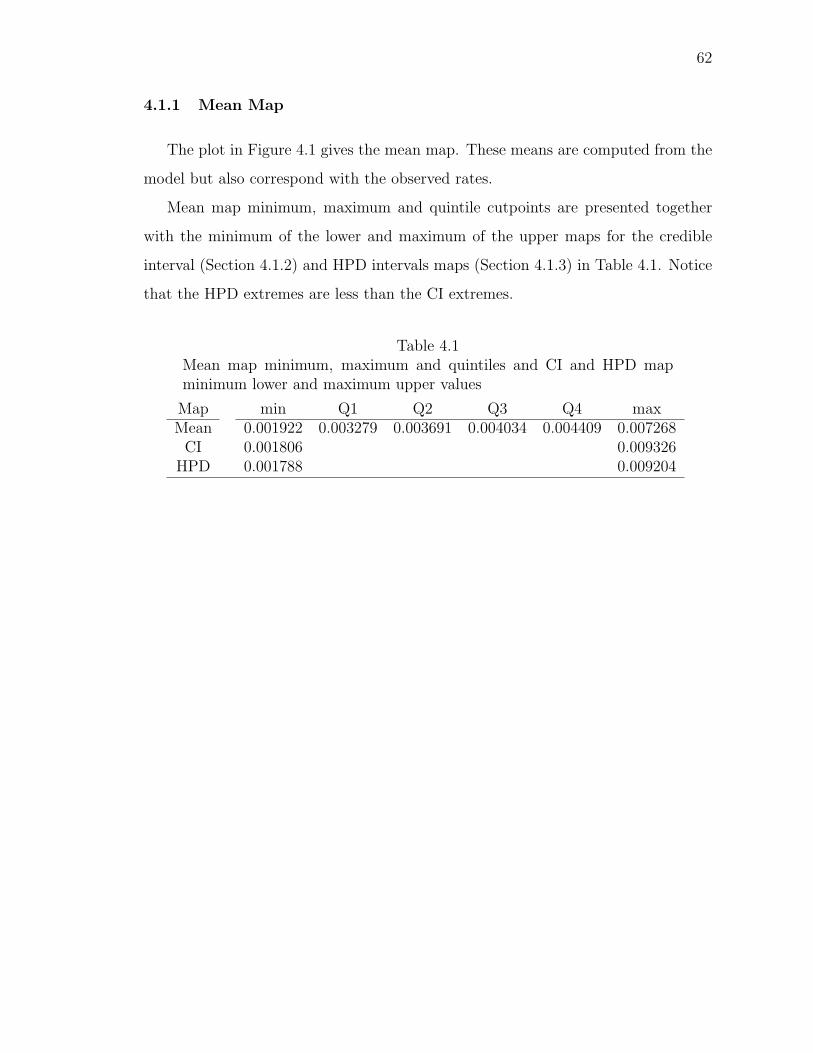
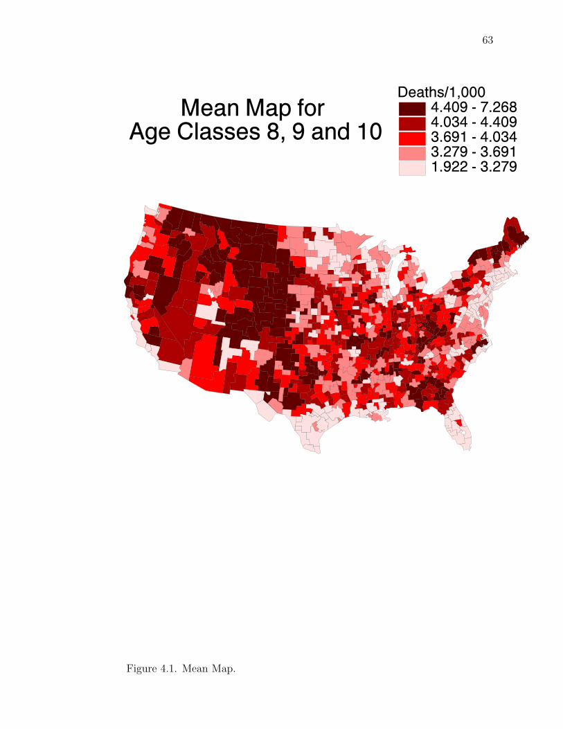
Health, 1995].

COPD attacks people at the height of their productive years, disabling them

with constant shortness of breath. It destroys their ability to earn a living, causes

frequent use of the health care system, and disrupts the lives of the victims’ family

13

members for as long as 20 years before death occurs [National Institutes of Health,

1995].

In 1990, COPD was the cause of approximately 16.2 million office visits to doctors

and 1.9 million hospital days. The economic costs of this disease are enormous. In

1989, an estimated $7 billion was spent for care of persons with COPD and another

$8 billion was lost to the economy by lost productivity due to morbidity and mortality

from COPD [National Institutes of Health, 1995].

1.6 Bayesian Method

For convenience we denote the number of HSAs by ` = 798. Let λ˜ = (λ1, . . . , λ`)′

denote the ensemble of mortality rate parameters, d˜ = (d1, . . . , d`)′ denote the deaths

and n˜ = (n1, . . . , n`)′ the population sizes which are known. We ignore the covariates

momentarily. In the Bayesian view, given λ˜, the deaths have a distribution; given

hyperparameters, λ˜ have a distribution (hyperparameters are parameters of this dis-

tribution), and finally the hyperparameters have a distribution. This is a hierarchical

Bayesian model. Note that unlike in non-Bayesian inference, λ˜ is a random vector.

Then, using Bayes’ theorem and some integration, the joint posterior density of λ˜ is

π(λ˜| d˜). Note that the key idea in Bayesian statistics is that all information about

λ˜ resides in π(λ˜| d˜). Also, it is important to note that the components of λ˜ are

correlated a posteriori. The posterior mean map is obtained by drawing the choro-

pleth map for the posterior means of each λi, i = 1, . . . , `. Clearly, this ignores the

inherrent correlation among the components of λ˜, and this is one additional obvious

short-comings of presenting the posterior mean map alone. One needs to construct

a map simultaneously across the areas (i.e., incorporate the correlation). It is the

simultaneous interval map that plots the joint posterior density over the surface

π(λ˜| d˜) providing a region in `-dimensional space that includes this correlation (i.e.,

the synergism or antagonism over the components of λ˜).

14

1.7 Thesis Overview

In the current chapter, by way of providing an introduction, we discussed choro-

pleth maps, small area mapping, models and methods, the source of the data and

discussed briefly the Bayesian method.

In Chapter 2 we discuss interval estimation, detailing all the intervals we em-

ploy, and develop the Single-γ Method and Double-γ Method simultaneous intervals.

These two methods are used to construct simultaneous intervals from the optimal

individual highest posterior density (HPD) intervals to ensure joint simultaneous

coverage of 100(1− α)%.

In Chapter 3 we discuss the Poisson-gamma hierarchical regression model and

the construction of intervals in this model context. Therefore, in addition to rate

parameter estimation, we describe an approach to present variability in choropleth

maps by constructing simultaneous intervals from the optimal individual highest pos-

terior density (HPD) intervals to ensure joint simultaneous coverage of 100(1− α)%.

The result provides three maps (estimate with two bands). Both methods exhibit

the main feature of multiplying the lower bound and dividing the upper bound of

the individual HPD intervals by parameters 0 < γ1, γ2 < 1 to “stretch” the interval

until the simultaneous probability content is 100(1− α)%. In Appendix A we give

an overview of the statistical methodology used in this research. In Appendix B we

give details and explanations for mathematical results in Chapter 3.

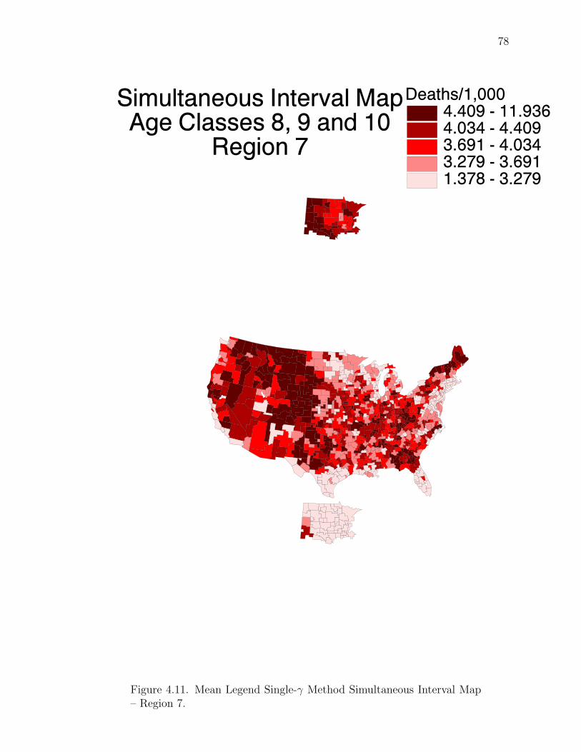
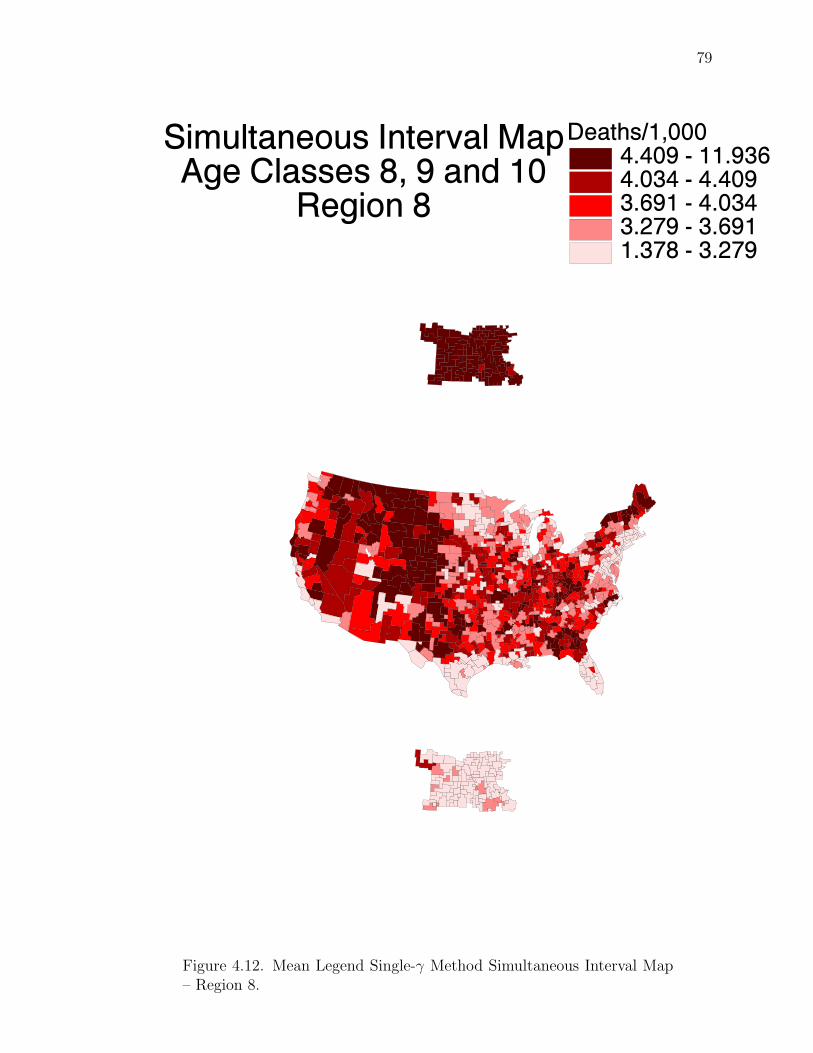
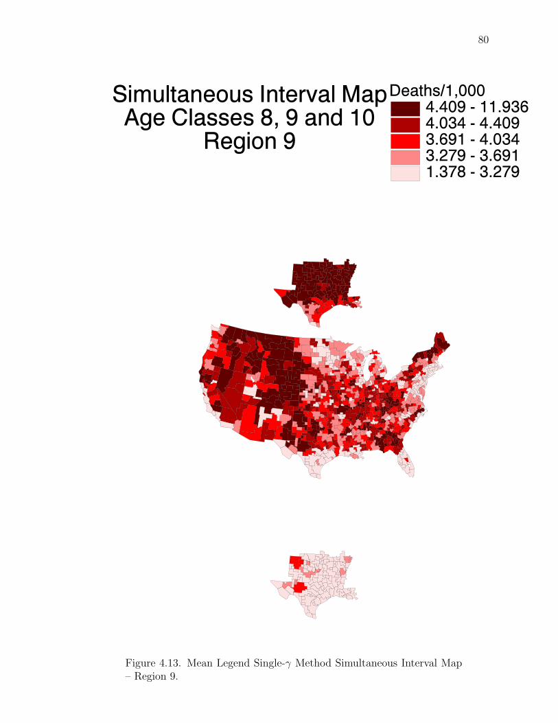
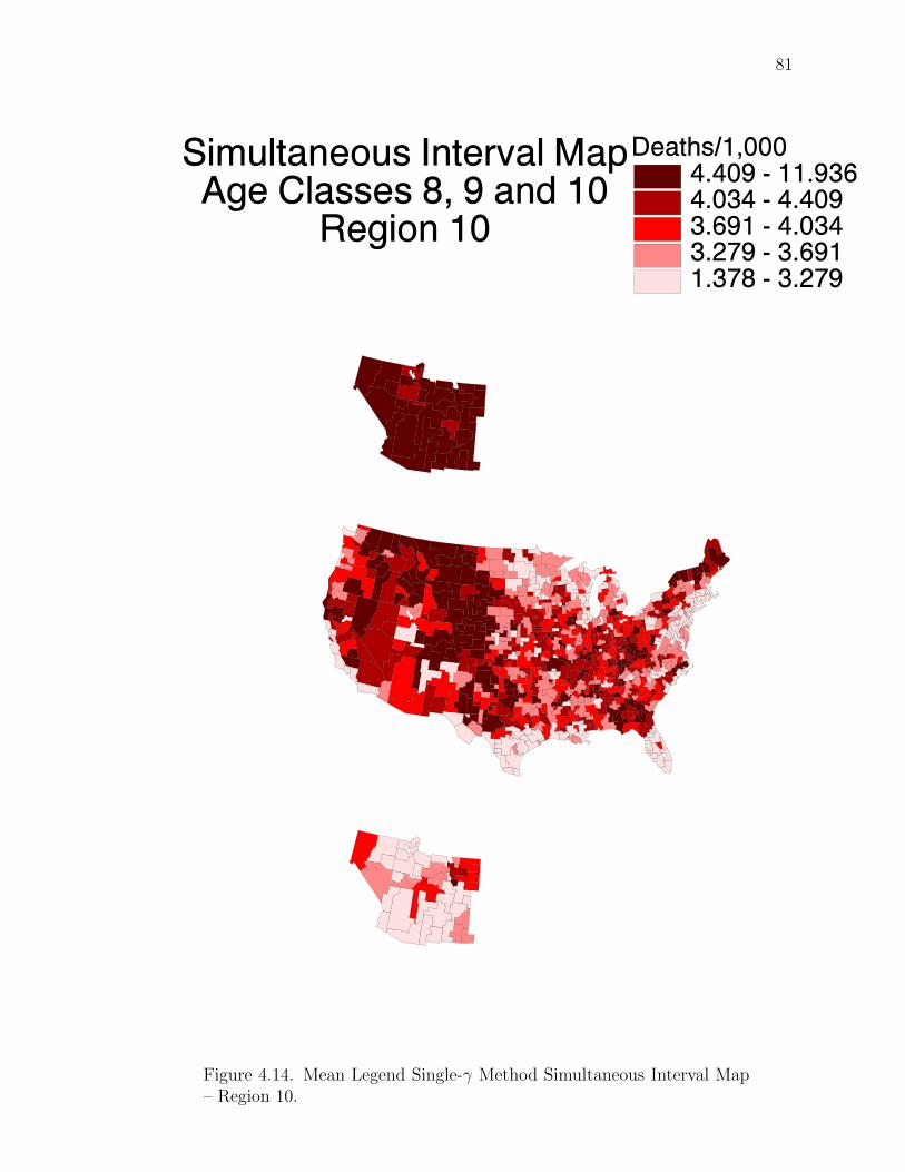
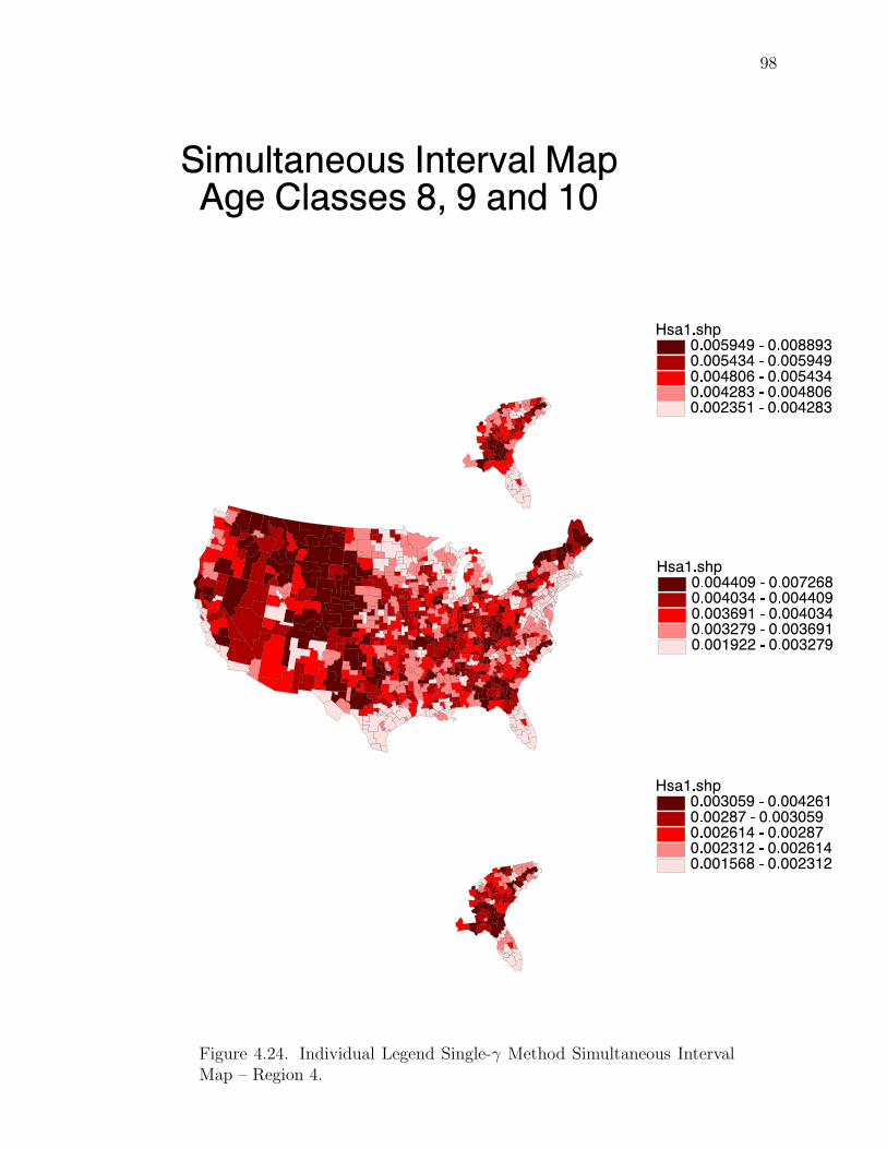
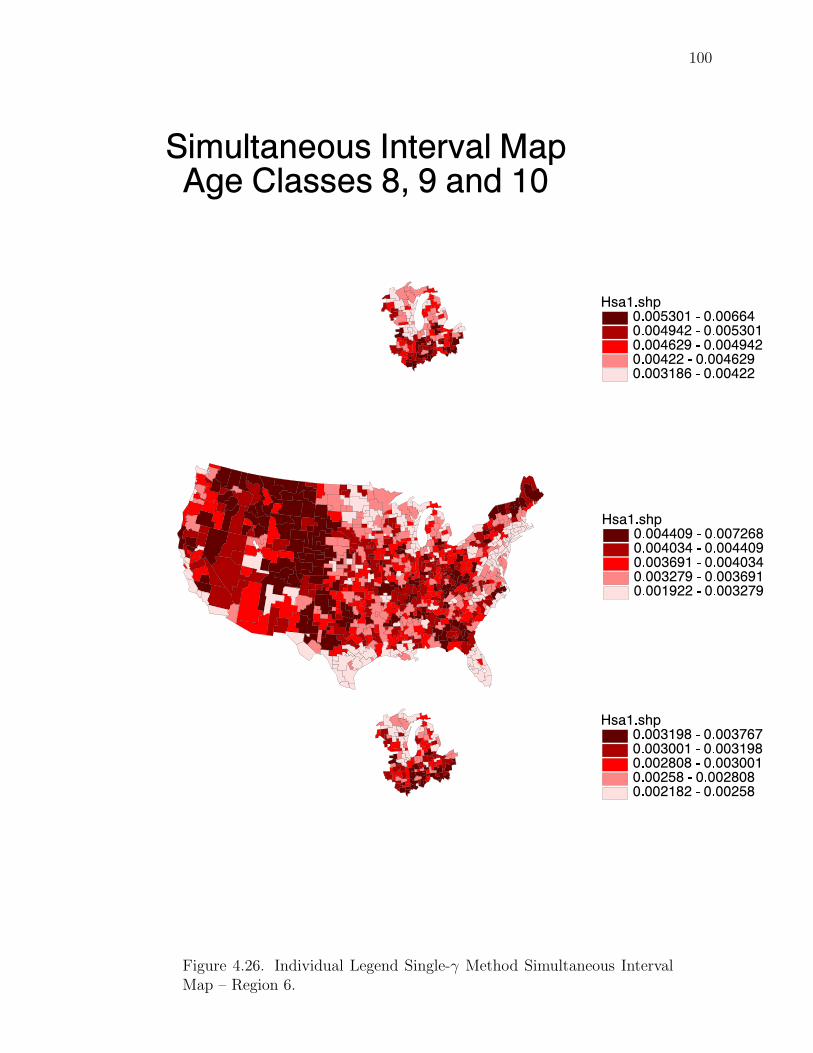
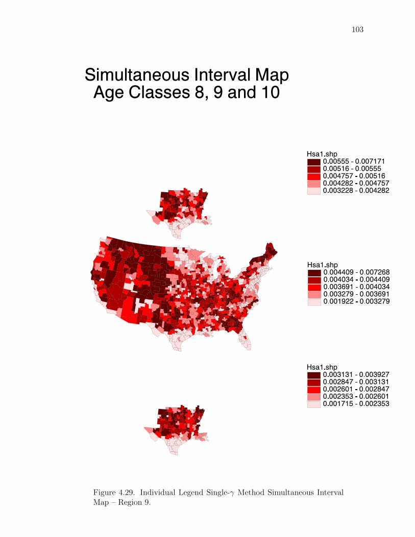
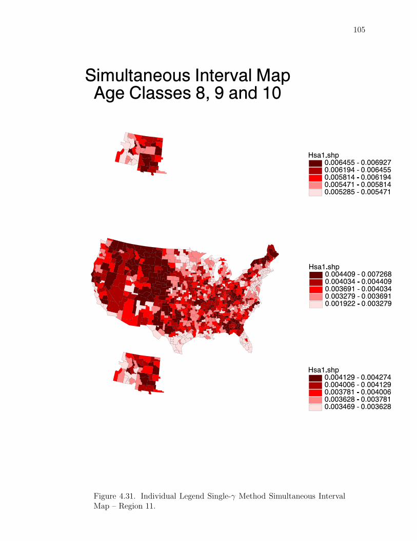
In Chapter 4 we present choropleth maps and the results from the simultaneous

interval methods. These include interval maps and difference maps and tables, both

novel methods of describing variation in maps.

For illustrative purposes we apply our methods to chronic obstructive pulmonary

disease (COPD) mortality rates from 1988–92, subset White Males age group 65

and older, for the continental United States for the 798 Health Service Areas (HSA).

In Chapter 5 we make conclusions from this research and provide suggestions for

extensions and further work on this topic.

15

2. SIMULTANEOUS INTERVAL ESTIMATION

The main idea of interval estimation is to take dataX1, . . . , Xn ∼ f(x˜| θ˜) and produce

a set C(X˜) ⊆ θ˜ that is a subset of the support of the parameter(s) of interest, θ˜.Ideally, this set will have two properties. First, the set should be more likely to

contain the true value of θ˜ than its complement. Second, the set should be small

in some sense. In many respects, the Bayesian approach to interval estimation is

simple and easily interpreted.

The purpose of using an interval estimator, rather than just a point estimator, is

to have some guarantee of capturing the parameter of interest. The interval estimator

combines both a point estimator and a measure of spread. The interval provides a

level of confidence, or assurance, that our assertion about the population parameters

is correct.

Common choices for the degree of confidence are 90%, 95% and 99%. The choice

of 95% is most common, since it seems to represent a good balance between precision

(as reflected in the width of the confidence interval) and reliability (as expressed by

the degree of confidence). Levels above 99% are generally unsatisfacotry because of

sensitivity to the assumed form of the tails of the distribution.

16

2.1 Review of Credible Intervals

2.1.1 Credible Intervals (CI)

Let f(θ| d˜) denote the posterior density of a parameter θ given data d˜.Definition 2.1.1 An interval (a, b) is called a 100(1 − α)% credible interval if its

posterior probability content is 1− α, that is,∫ ba f(θ| d˜) dθ = 1− α.

Credible intervals are not unique. Two credible intervals can exist such that

∫ b1

a1

f(θ| d˜) dθ =∫ b2

a2

f(θ| d˜) dθ = 1− α (2.1)

or

F (b1)− F (a1) = F (b2)− F (a2) = 1− α, (2.2)

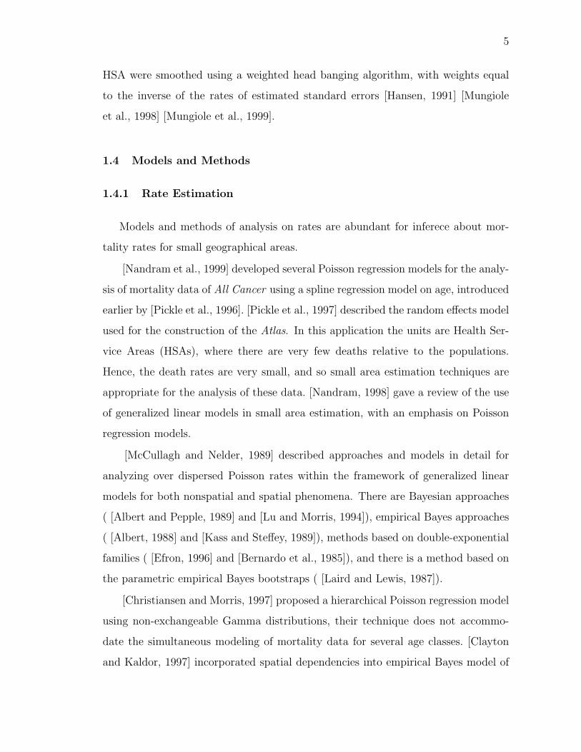
a1 6= a2 and b1 6= b2, where F (·) is the cdf. As an example the plot in Figure 2.1 gives

three 95% credible intervals for the Gamma(α, β) distribution, that is, f(x|α, β) =

1Γ(α)βαx

α−1e−x/β where 0 ≤ x < ∞ and α, β > 0, with α = 3 and β = 1. The first

interval (a1, b1) = (0.4360, 6.5989) covers from the 0.01 to 0.96 quantile, the second

interval (a2, b2) = (0.7462, 8.4059) covers from the 0.04 to 0.99 quantile, and the

third interval (acred, bcred) = (0.6187, 7.2247) covers from the 0.025 to 0.975 quantile.

Credible intervals are easy to construct. Typically, we construct credible intervals

with equal tail probabilities to their left and to their right. For a 100(1−α)% credible

interval, there is 100(α2)% probability in each tail. The plot in Figure 2.1 gives such

a 95% credible interval where the interval (acred, bcred) = (0.6187, 7.2247) covers from

the 0.025 to 0.975 quantile.

Interval Construction

There are two ways to construct credible intervals: numerical and sampling-

based.

17

Method 1 (Numerical) Let F (θ| d˜) =∫ θ−∞ f(t| d˜) dt be the cumulative distri-

bution function (cdf). Let F−1(.| d˜) be the inverse cdf. Then a = F−1(α2| d˜) and

b = F−1(1− α2| d˜) give the 100(1− α)% credible interval (a, b).

Method 2 (Sampling-based) Draw a random sample of 1,000 values from f(θ| d˜).Place the values in ascending order, θ(1) < θ(2) < . . . < θ(1000). Then an estimate

from these order statistics of the 95% credible interval is (θ(25), θ(976)). This method

is usually used in complex problems, and is the method used in this paper. This

method works well for large samples (i.e., about 1000).

2.1.2 Highest Posterior Density (HPD) Intervals

Not only should we be concerned with the probability content of the interval, but

we wish to use the interval with the highest posterior density.

Definition 2.1.2 A 100(1−α)% credible interval (a, b) is a highest posterior density

(HPD) interval if for any θ1 ∈ (a, b) and θ2 /∈ (a, b), f(θ1| d˜) ≥ f(θ2| d˜). In other

words, the height of any point of the density within the HPD interval is greater than

for any point outside the interval.

All candidate intervals must contain the mode. The 100(1 − α)% HPD interval

is unique for any unimodal posterior density. If the mode is on a boundary of the

posterior density, then that boundary is one of the end points in the interval. The

100(1− α)% HPD interval is the shortest interval with 100(1− α)% coverage.

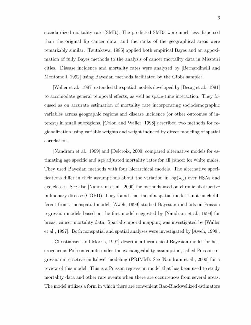
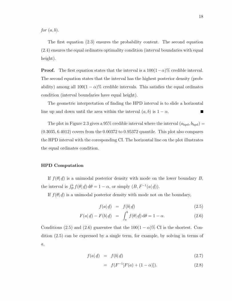
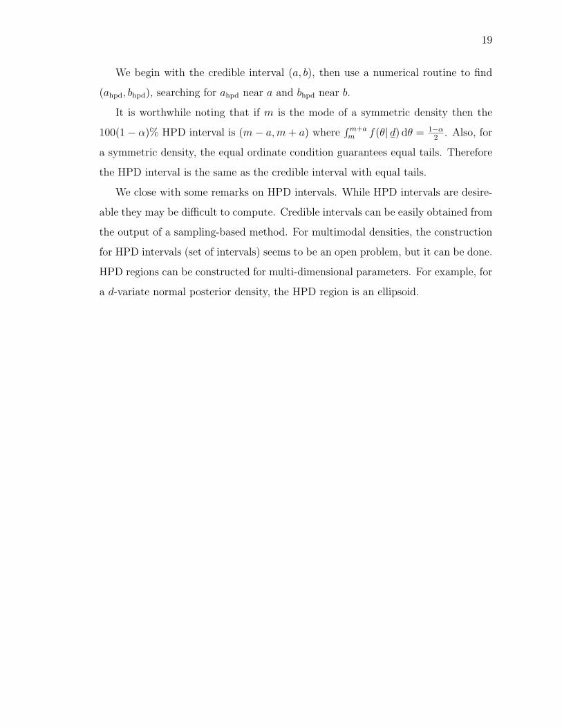
The plots in Figure 2.2 give examples of HPD intervals on densities with a mode

on the boundary and not on the boundary.

Theorem 2.1.1 For a unimodal posterior density the 100(1−α)% HPD interval is

obtained by solving the two equations∫ b

af(θ| d˜) dθ = 1− α (2.3)

f(a| d˜) = f(b| d˜) (2.4)

18

for (a, b).

The first equation (2.3) ensures the probability content. The second equation

(2.4) ensures the equal ordinates optimality condition (interval boundaries with equal

height).

Proof. The first equation states that the interval is a 100(1−α)% credible interval.

The second equation states that the interval has the highest posterior density (prob-

ability) among all 100(1− α)% credible intervals. This satisfies the equal ordinates

condition (interval boundaries have equal height).

The geometric interpretation of finding the HPD interval is to slide a horizontal

line up and down until the area within the interval (a, b) is 1− α.

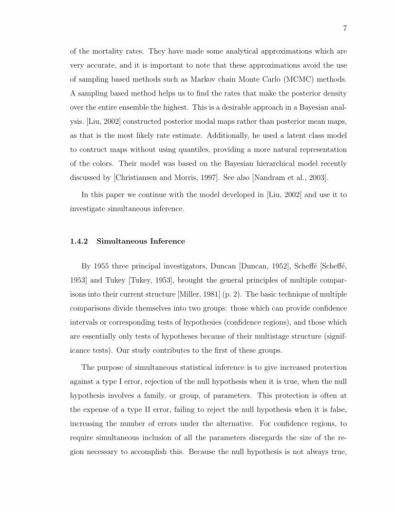
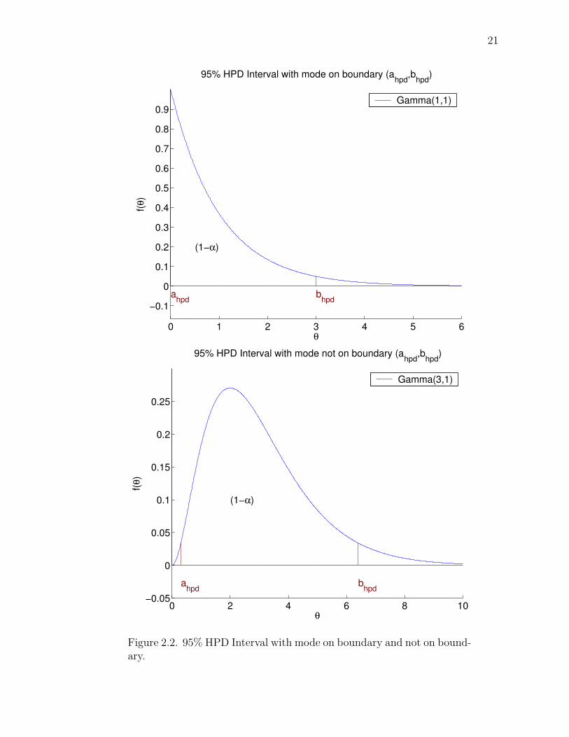
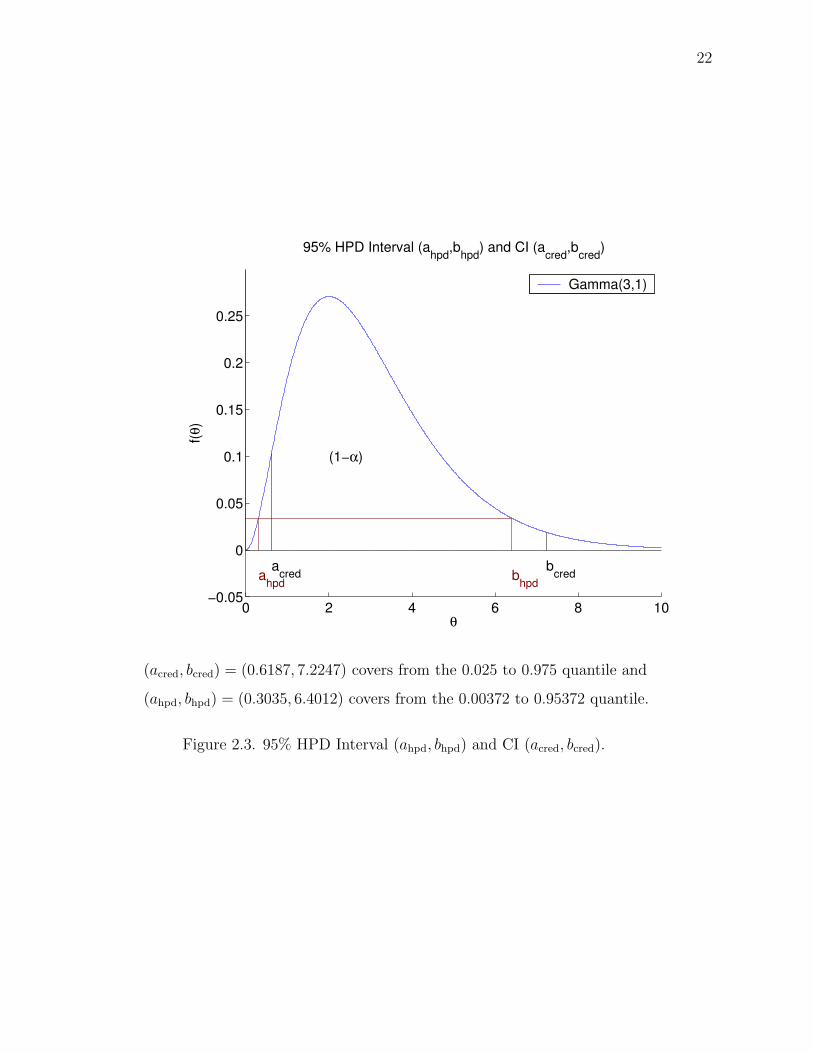
The plot in Figure 2.3 gives a 95% credible interval where the interval (ahpd, bhpd) =

(0.3035, 6.4012) covers from the 0.00372 to 0.95372 quantile. This plot also compares

the HPD interval with the coresponding CI. The horizontal line on the plot illustrates

the equal ordinates condition.

HPD Computation

If f(θ| d˜) is a unimodal posterior density with mode on the lower boundary B,

the interval is∫ aB f(θ| d˜) dθ = 1− α, or simply (B,F−1(a| d˜)).

If f(θ| d˜) is a unimodal posterior density with mode not on the boundary,

f(a| d˜) = f(b| d˜) (2.5)

F (a| d˜)− F (b| d˜) =∫ b

af(θ| d˜) dθ = 1− α. (2.6)

Conditions (2.5) and (2.6) guarentee that the 100(1− α)% CI is the shortest. Con-

dition (2.5) can be expressed by a single term, for example, by solving in terms of

a,

f(a| d˜) = f(b| d˜) (2.7)

= f(F−1[F (a) + (1− α)]). (2.8)

19

We begin with the credible interval (a, b), then use a numerical routine to find

(ahpd, bhpd), searching for ahpd near a and bhpd near b.

It is worthwhile noting that if m is the mode of a symmetric density then the

100(1− α)% HPD interval is (m− a,m+ a) where∫m+am f(θ| d˜) dθ = 1−α

2. Also, for

a symmetric density, the equal ordinate condition guarantees equal tails. Therefore

the HPD interval is the same as the credible interval with equal tails.

We close with some remarks on HPD intervals. While HPD intervals are desire-

able they may be difficult to compute. Credible intervals can be easily obtained from

the output of a sampling-based method. For multimodal densities, the construction

for HPD intervals (set of intervals) seems to be an open problem, but it can be done.

HPD regions can be constructed for multi-dimensional parameters. For example, for

a d-variate normal posterior density, the HPD region is an ellipsoid.

20

0 2 4 6 8 10−0.05

0

0.05

0.1

0.15

0.2

0.25

θ

f(θ)

Three 95% Credible Intervals (a1,b

1), (a

2,b

2), (a

cred,b

cred)

a1

b1

a2

b2

acred

bcred

(1−α)

Gamma(3,1)

(a1, b1) = (0.4360, 6.5989) covers from the 0.01 to 0.96 quantile,

(a2, b2) = (0.7462, 8.4059) covers from the 0.04 to 0.99 quantile, and

(acred, bcred) = (0.6187, 7.2247) covers from the 0.025 to 0.975 quantile.

Figure 2.1. Credible intervals are not unique.

21

0 1 2 3 4 5 6

−0.1

0

0.1

0.2

0.3

0.4

0.5

0.6

0.7

0.8

0.9

θ

f(θ)

95% HPD Interval with mode on boundary (ahpd

,bhpd

)

ahpd

bhpd

(1−α)

Gamma(1,1)

0 2 4 6 8 10−0.05

0

0.05

0.1

0.15

0.2

0.25

θ

f(θ)

95% HPD Interval with mode not on boundary (ahpd

,bhpd

)

ahpd

bhpd

(1−α)

Gamma(3,1)

Figure 2.2. 95% HPD Interval with mode on boundary and not on bound-ary.

22

0 2 4 6 8 10−0.05

0

0.05

0.1

0.15

0.2

0.25

θ

f(θ)

95% HPD Interval (ahpd

,bhpd

) and CI (acred

,bcred

)

acred

bcreda

hpdb

hpd

(1−α)

Gamma(3,1)

(acred, bcred) = (0.6187, 7.2247) covers from the 0.025 to 0.975 quantile and

(ahpd, bhpd) = (0.3035, 6.4012) covers from the 0.00372 to 0.95372 quantile.

Figure 2.3. 95% HPD Interval (ahpd, bhpd) and CI (acred, bcred).

23

2.2 Simultaneous Intervals

Why do we need simultaneous intervals? Consider two parameters µ1 and µ2.

Let a 95% CI for µ1 be (a1, b1) and a 95% CI for µ2 be (a2, b2). Then the intersection

(a1, b1)∩ (a2, b2) does not form a set giving a 95% credible interval (i.e., smaller than

95%). So all we need is to lengthen these individual intervals in an optimal manner.

2.2.1 Boole’s inequality

Bonferroni’s inequality, P (A ∩ B) ≥ P (A) + P (B) − 1, allows us to bound

the probability of a simultaneous event (the intersection) in terms of the proba-

bilities of the individual events [Miller, 1981] (p. 8). Boole’s inequality, P (∩ni=1Ai) ≥∑n

i=1 P (Ai)−(n−1), gives a more general form of the Bonferroni inequality, allowing

for more than two events. This method gives a meaningful result when the number

of events is small and the probabilities of the individual events are sufficiently large.

In our case, we wish to have a simultaneous interval containing 798 individual

intervals, an extremely large quantity of events. By Boole’s inequality, we wish the

intersection of the individual intervals to be at least 0.95. We have P (∩ni=1Ai) ≥∑n

i=1 P (Ai) − (n − 1) = 0.95,∑n

i=1 P (Ai) = 0.95 + (n − 1), 798P (A) ≤ 0.95 +

(798 − 1) (since each area should have the same probability content), P (A) ≤0.95+797

798= 0.999937343

.= 0.99994. Therefore, the probability content of each in-

dividual event’s interval is bounded above by 0.99994. The credible interval is

(F−1(0.00003), F−1(0.99997)) for two-tailed, and (F−1(0), F−1(0.99994)) for one-

tailed. Computations break down at this strict lower bound limit given by Boole’s

inequality.

We should not apply Boole’s correction directly to our problem since it is strictly

an upper bound (a worst-case scenario). As these individual intervals are covering

nearly the entire support of the individual densities, they are somewhat meaningless.

The true individual probabilities will most likely lie somewhere between 0.95 and the

above 0.99994. A more exact method is preferred.

24

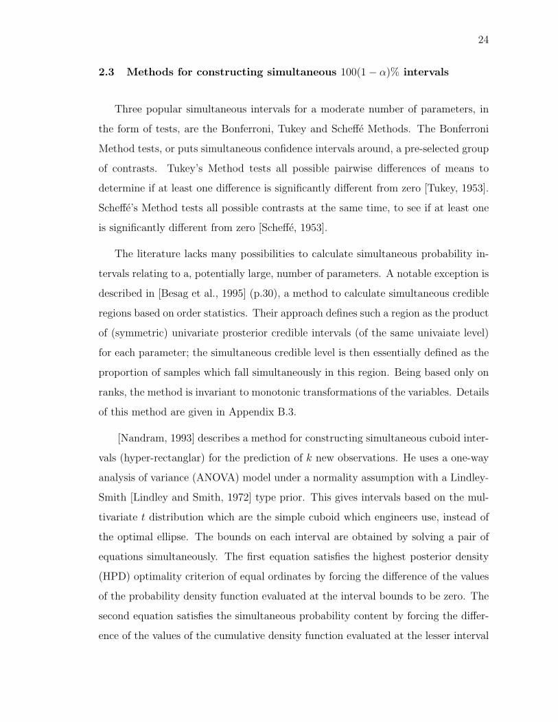
2.3 Methods for constructing simultaneous 100(1− α)% intervals

Three popular simultaneous intervals for a moderate number of parameters, in

the form of tests, are the Bonferroni, Tukey and Scheffe Methods. The Bonferroni

Method tests, or puts simultaneous confidence intervals around, a pre-selected group

of contrasts. Tukey’s Method tests all possible pairwise differences of means to

determine if at least one difference is significantly different from zero [Tukey, 1953].

Scheffe’s Method tests all possible contrasts at the same time, to see if at least one

is significantly different from zero [Scheffe, 1953].

The literature lacks many possibilities to calculate simultaneous probability in-

tervals relating to a, potentially large, number of parameters. A notable exception is

described in [Besag et al., 1995] (p.30), a method to calculate simultaneous credible

regions based on order statistics. Their approach defines such a region as the product

of (symmetric) univariate prosterior credible intervals (of the same univaiate level)

for each parameter; the simultaneous credible level is then essentially defined as the

proportion of samples which fall simultaneously in this region. Being based only on

ranks, the method is invariant to monotonic transformations of the variables. Details

of this method are given in Appendix B.3.

[Nandram, 1993] describes a method for constructing simultaneous cuboid inter-

vals (hyper-rectanglar) for the prediction of k new observations. He uses a one-way

analysis of variance (ANOVA) model under a normality assumption with a Lindley-

Smith [Lindley and Smith, 1972] type prior. This gives intervals based on the mul-

tivariate t distribution which are the simple cuboid which engineers use, instead of

the optimal ellipse. The bounds on each interval are obtained by solving a pair of

equations simultaneously. The first equation satisfies the highest posterior density

(HPD) optimality criterion of equal ordinates by forcing the difference of the values

of the probability density function evaluated at the interval bounds to be zero. The

second equation satisfies the simultaneous probability content by forcing the differ-

ence of the values of the cumulative density function evaluated at the lesser interval

25

bound from the greater interval bound to be 1− α. Thus the cuboids are optimized

by constructing the smallest such k-dimensional cuboid by using HPD intervals in

each dimension.

The method presented in our paper is an extention of the method of [Nandram,

1993]. Two main differences are that we consider a large number of parameters

` = 798, where he considered up to k = 10 predictions, and we use a Poisson-gamma

hierarchical model instead of an ANOVA model under normality.

We propose to construct simultaneous 100(1 − α)% intervals by “stretching”

individual HPD intervals until the desired content is obtained, together with an

optimality criterion. The simultaneous intervals are defined as the product of the

univariate intervals, which are by construction restricted to be hyper-rectanglar.

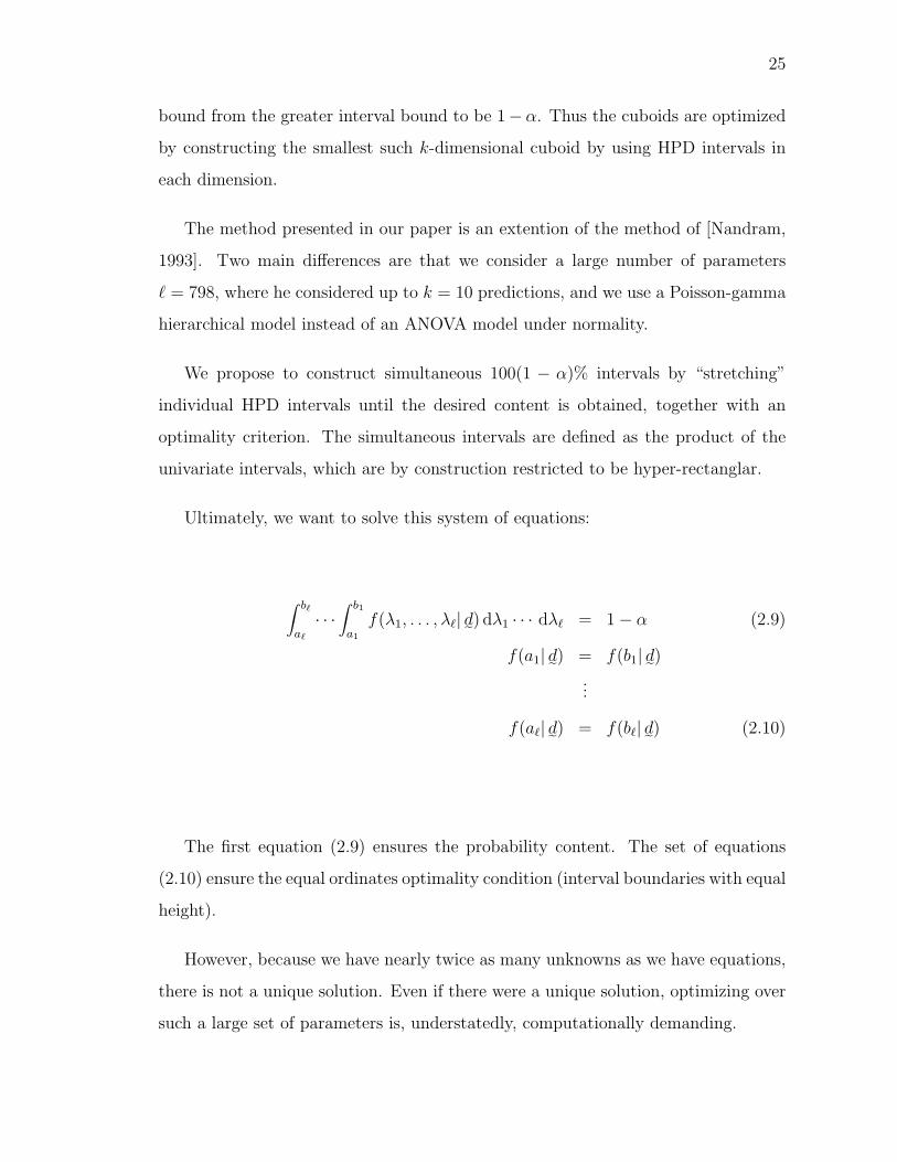
Ultimately, we want to solve this system of equations:

∫ b`

a`

· · ·∫ b1

a1

f(λ1, . . . , λ`| d˜) dλ1 · · · dλ` = 1− α (2.9)

f(a1| d˜) = f(b1| d˜)...

f(a`| d˜) = f(b`| d˜) (2.10)

The first equation (2.9) ensures the probability content. The set of equations

(2.10) ensure the equal ordinates optimality condition (interval boundaries with equal

height).

However, because we have nearly twice as many unknowns as we have equations,

there is not a unique solution. Even if there were a unique solution, optimizing over

such a large set of parameters is, understatedly, computationally demanding.

26

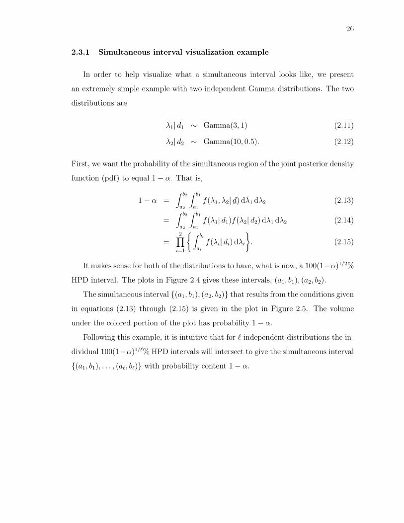
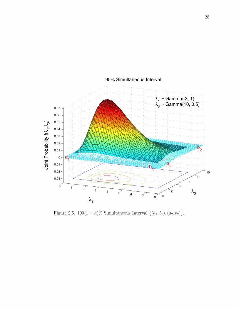
2.3.1 Simultaneous interval visualization example

In order to help visualize what a simultaneous interval looks like, we present

an extremely simple example with two independent Gamma distributions. The two

distributions are

λ1| d1 ∼ Gamma(3, 1) (2.11)

λ2| d2 ∼ Gamma(10, 0.5). (2.12)

First, we want the probability of the simultaneous region of the joint posterior density

function (pdf) to equal 1− α. That is,

1− α =∫ b2

a2

∫ b1

a1

f(λ1, λ2| d˜) dλ1 dλ2 (2.13)

=∫ b2

a2

∫ b1

a1

f(λ1| d1)f(λ2| d2) dλ1 dλ2 (2.14)

=2∏

i=1

∫ bi

ai

f(λi| di) dλi

. (2.15)

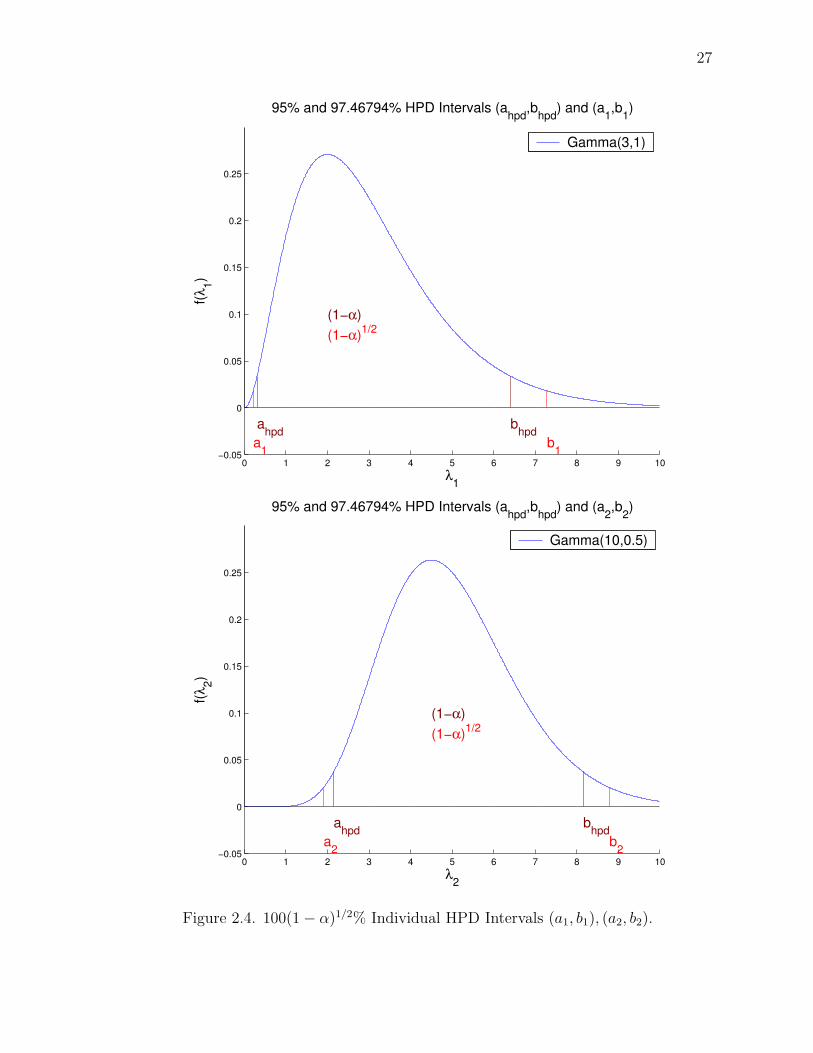
It makes sense for both of the distributions to have, what is now, a 100(1−α)1/2%

HPD interval. The plots in Figure 2.4 gives these intervals, (a1, b1), (a2, b2).

The simultaneous interval (a1, b1), (a2, b2) that results from the conditions given

in equations (2.13) through (2.15) is given in the plot in Figure 2.5. The volume

under the colored portion of the plot has probability 1− α.

Following this example, it is intuitive that for ` independent distributions the in-

dividual 100(1−α)1/`% HPD intervals will intersect to give the simultaneous interval

(a1, b1), . . . , (a`, b`) with probability content 1− α.

27

0 1 2 3 4 5 6 7 8 9 10−0.05

0

0.05

0.1

0.15

0.2

0.25

λ1

f(λ1)

95% and 97.46794% HPD Intervals (ahpd

,bhpd

) and (a1,b

1)

ahpd

bhpd

(1−α)

a1

b1

(1−α)1/2

Gamma(3,1)

0 1 2 3 4 5 6 7 8 9 10−0.05

0

0.05

0.1

0.15

0.2

0.25

95% and 97.46794% HPD Intervals (ahpd

,bhpd

) and (a2,b

2)

λ2

f(λ2)

ahpd

bhpd

(1−α)

a2

b2

(1−α)1/2

Gamma(10,0.5)

Figure 2.4. 100(1− α)1/2% Individual HPD Intervals (a1, b1), (a2, b2).

28

0 1 2 3 4 5 6 7 8 02

46

810

−0.03

−0.02

−0.01

0

0.01

0.02

0.03

0.04

0.05

0.06

0.07

b2

λ2

a2

λ1 ~ Gamma( 3, 1)

λ2 ~ Gamma(10, 0.5)

b1

95% Simultaneous Interval

λ1

a1

Join

t Pro

babi

lity

f(λ1,λ

2)

Figure 2.5. 100(1− α)% Simultaneous Interval (a1, b1), (a2, b2).

29

2.4 Single-γ Method Simultaneous 100(1− α)% interval

One method to simplify our goal in equation (2.9) is to provide one parameter to

operate on the individual HPD intervals. Let 0 < γ < 1 be a “stretching” factor on

the HPD interval (ai, bi), giving the stretched interval higher content than the initial

interval,

∫ bi/γ

γai

f(λi| di) dλi ≥∫ bi

ai

f(λi| di) dλi. (2.16)

In this way we can begin with an optimized condition of HPD intervals (ai, bi) and

stretch them until the desired content is obtained. Thus our goal using the Single-γ

Method is to satisfy the equation

∫ b`/γ

γa`

· · ·∫ b1/γ

γa1

f(λ1, . . . , λ`| d˜) dλ1 · · · dλ` = 1− α (2.17)

for i = 1, . . . , `.

2.4.1 Single-γ Method Computations

The goal is to optimize the following equation (2.18) by determining the value

for γ such that minγ F (γ) approaches zero.

F (γ) =

∣∣∣∣∣∫ b`/γ

γa`

· · ·∫ b1/γ

γa1

f(λ1, . . . , λ`| d˜) dλ1 · · · dλ` − (1− α)

∣∣∣∣∣ (2.18)

The following theorem shows that the Single-γ Method has a unique solution

with the correct probability content in equation (2.17).

Theorem 2.4.1 Given a set of HPD credible intervals A′i = λi : ai < λi < bi,

i = 1, . . . , `, defined on a set of densities with positive support and given the trans-

formation Ai = λi : γai < λi < bi/γ, there is a unique γ satisfying P (∩ì=1Ai| d˜) =

1− α, where d˜ is the data.

Proof. Let A′i = λi : ai < λi < bi be the individual 100(1 − α)% HPD credible

interval defined on a set of densities with positive support, P (A′i| di) = 1 − α, i =

30

1, . . . , `. We will use γ as a “stretching” factor for this interval to allow us to find a

unique solution for a simultaneous interval.

Let Ai = λi : γai < λi < bi/γ be the stretched individual HPD interval with

P (Ai| di) ≥ 1− α, i = 1, . . . , `, and P (∩ì=1Ai| di) = 1− α be the probability of the

intersection. Observe that as γ decreases to 0, each Ai is a sequence of increasing

sets so that ∩ì=1Ai| di is a sequence of increasing sets. So, by the continuity

theorem,

limγ→0

P (∩ì=1Ai| di) = P

(limγ→0

∩ì=1Ai| di

)= P (λ˜ ∈ <`

+| d˜), λ˜ = (λ1, . . . , λ`)′

= 1.

That is, at the limit, as γ goes to 0, the sequence of increasing sets ∩ì=1Ai| di

encompasses the entire space <`+, the positive `-dimensional reals. Also, at γ =

1, P (∩ì=1Ai| di) < P (A′

i| di) = 1 − α. Thus, as γ → 0, P (∩ì=1Ai| di) increases

smoothly from a value less than 1− α to 1. Therefore, there is a unique solution to

P (∩ì=1Ai| di) = 1− α in terms of γ.

31

2.5 Double-γ Method Simultaneous 100(1− α)% interval

One method to simplify our goal set in equations (2.9) and (2.10) is to provide

two parameters to operate on the individual HPD intervals. Let 0 < γ1 < 1 and

0 < γ2 < 1 be “stretching” factors on the HPD interval (ai, bi), giving the stretched

interval higher content than the initial interval,

∫ bi/γ2

γ1ai

f(λi| d˜) dλi ≥∫ bi

ai

f(λi| d˜) dλi. (2.19)

In this way we can begin with an optimized condition of HPD intervals (ai, bi),

and stretch them until the desired content is obtained together with an ordinate

optimality criterion. Thus our goal using the Double-γ Method is to satisfy the two

equations

∫ b`/γ2

γ1a`

· · ·∫ b1/γ2

γ1a1

f(λ1, . . . , λ`| d˜) dλ1 · · · dλ` = 1− α (2.20)

f(γ1ai| di) = f(bi/γ2| di) (2.21)

for i = 1, . . . , `. Note that we have two parameters and have at least two equa-

tions, depending on how we wish to formulate our ordinate optimization criterion in

equation (2.21). These two equations may lead to different values of γ1, γ2 when

optimized. Therefore, when we must choose, the content (2.20) takes precedence.

2.5.1 Double-γ Method Computations

The goal is to optimize the following equation (2.22) by determining values for

γ1, γ2 such that minγ1,γ2 F (γ1, γ2) approaches zero. The value of the ordinate opti-

mality criterion S∗o is determined by the methods described in Section 2.6.

F (γ1, γ2) =

∣∣∣∣∣∫ b`/γ2

γ1a`

· · ·∫ b1/γ2

γ1a1

f(λ1, . . . , λ`| d˜) dλ1 · · · dλ` − (1− α)

∣∣∣∣∣+|S∗o | (2.22)

32

2.6 Equal Ordinate condition optimization criterion

Our goal is to construct simultaneous HPD intervals for a large number of small

areas. To obtain the precise properties of HPD intervals (see definition 2.1.2) in the

simultaneous case, equation (2.9) and set of equations (2.10) need to be solved. As

stated earlier (Section 2.3), this requires the solution for more unknowns than we

have equations.

To make this situation solvable, we introduce approximations to the exact opti-

mality condition from equations (2.10) which will be computed from a function of

the ordinates in (2.21).

A number of ordinate optimization criterion have been considered. For each of

these criteria, the object during optimization is to bring the value of the expression

to zero.

2.6.1 Maximum Relative Difference Criterion

To calculate the Maximum Relative Difference, evaluate the ordinates for each of

the ` areas, and take the ratio of the larger average over the lesser average to obtain

the larger ratio. This ratio will be one when the ordinates are equal. Subtract one

from the ratio and take absolute value as a measure of the difference between these

ordinates. Finally, find the maximum value over all ` areas. Set this equal to S∗1 and

use in equation (2.22), where

S∗1 = maxi∈1,...,`

[∣∣∣∣∣max

f(γ1ai| di)

f(bi/γ2| di),f(bi/γ2| di)

f(γ1ai| di)

− 1

∣∣∣∣∣]. (2.23)

2.6.2 Average Relative Difference Criterion

To calculate the Average Relative Difference, evaluate the ordinates for each of

the ` areas, and take the ratio of the absolute difference of the left and right ordinates

33

over their sum. This ratio will be zero when the ordinates are equal. Average these

over all ` areas. Set this equal to S∗2 and use in equation (2.22), where

S∗2 = `−1∑i=1

|f(γ1ai| di)− f(bi/γ2| di)|f(γ1ai| di) + f(bi/γ2| di)

. (2.24)

This method uses the ratio of the difference to the sum to adjust for possibly large

differences in ordinate magnitude between areas. This gives each area equal weight

in the optimization.

2.6.3 Average Absolute Difference Criterion

To calculate the Average Absolute Difference, evaluate the ordinates for each of

the ` areas, and take the absolute difference of the left and right ordinates. This

difference will be zero when the ordinates are equal. Average these over all ` areas.

Set this equal to S∗3 and use in equation (2.22), where

S∗3 = `−1∑i=1

|f(γ1ai| di)− f(bi/γ2| di)| . (2.25)

This method does not adjust for possibly large differences in ordinate magnitude

between areas. A few areas are likely to dominate this optimization.

34

35

3. SIMULTANEOUS INTERVALS FOR A HIERARCHICAL

POISSON MODEL

3.1 The Poisson-Gamma Hierarchical Regression Model

In this chapter we describe the Poisson-gamma hierarchical Bayesian model and

how to fit it using the Metropolis-Hastings sampler.

Let λi denote the mortality rate for HSA i, i = 1, . . . , `, where ` = 798. The

observations consist of the number of deaths di and the population size ni for HSA

i, i = 1, . . . , `. To link the di and the ni to the mortality rate λi, we assume

di|λiind∼ Poisson(niλi), i = 1, . . . , `. (3.1)

Under this model the maximum likelihood estimator (MLE) of λi is ri = di/ni,

i = 1, . . . , `, the observed mortality rate.

It is standard to estimate the λi by “borrowing strength” across the 798 HSAs.

Four potential risk factors were selected in [Nandram et al., 2000] for COPD. These

risk factors, used as covariates, help to explain the spatial patterns of COPD and its

constituent diseases (asthma, chronic bronchitis and emphysema). These are recalled

in Table 3.1, and maps are given in Figure 3.1. All the 95% credible intervals do

not contain zero, meaning they are all significant [Liu, 2002]. (Population sizes and

death counts may also be of interest; these are given in Figure 3.2.)

β1, the coefficient for white male lung cancer mortality rate is positive. This con-

firms [Morris and Munasinghe, 1994]; those places where more people smoke

tend to have a higher COPD mortality rate.

β2, the coefficient for population density is negative, this confirms [Nandram et al.,

2000]. The possible reason might be, those places with a high population

36

density usually have better medical services, and when there is an emergency

people living in a remote area are more likely to be delayed by the long travel

to the nearest hospital.

β3, the coefficient for elevation is positive. This confirms that extreme climatic

conditions aggravate existing asthma and bronchitis [Bates, 1989], as is living

at high altitudes because of the reduced oxygen supply [Schoene, 1999].

β4, the coefficient for the annual rainfall level is negative. As claimed before, re-

peated exposure to particulate matter and other air pollutants, primarily from

traffic exhaust and coal-burning power plants, can aggravate existing lung con-

ditions and can even cause death [English et al., 1999] [Sunyer et al., 2000]. In

particular, small airborne particles such as SO2 found in urban air pollution

can be deposited deep in the lungs, causing severe pulmonary effects [Sunyer

et al., 2000] [Schwartz and Neas, 2000]. Aerosolized toxins and viruses can

be inhaled in dusty environments, causing pulmonary effects [National Center

for Health Statistics, 1998]. Rainfall, on the contrary, can lower the density

of airborne particles and dust in the air, thus lower the chance of catching a

pulmonary disease.

We link these covariates to the mortality rate, λi. Thus, letting x˜i = (1, xi,1, . . . , xi,p−1)′

denote the vector of (p − 1) covariates and an intercept, and fitting the covariates

in the regression model (with mortality rate λi as the response variable) we assume

that

λi|α, β˜ ind∼ Gamma(α, αe−x˜′iβ˜), i = 1, . . . , `. (3.2)

Observe that in this model log(E(λi|α, β˜)) = x˜′iβ˜ and√α is the coefficient of varia-

tion of the λi. (Throughout, by T ∼ Gamma(a, b) we mean fT (t) = bata−1e−bt/Γ(a), t ≥

0.)

37

Figure 3.1. Regression Covariate (Risk Factor) Maps.

38

Table 3.1Regression Covariates (Risk Factors)

Covariates (x˜) Coefficients (β˜) Risk Factor

x0 (≡ 1) β0 Intercept

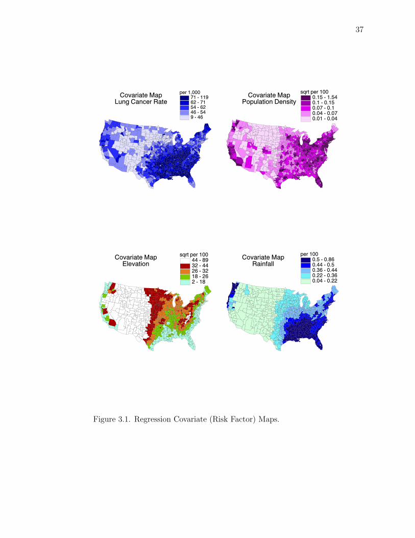
x1 β1 white male lung cancer rate per 1,000 population

x2 β2 square root of (population density/104)

x3 β3 square root of (elevation/104)

x4 β4 (annual rainfall/100)

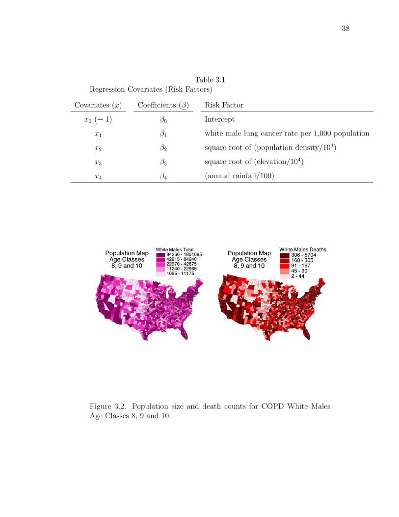
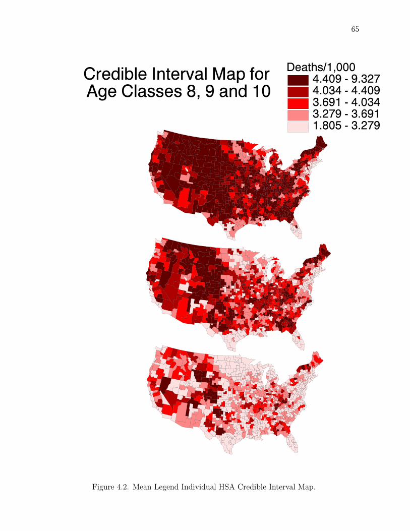
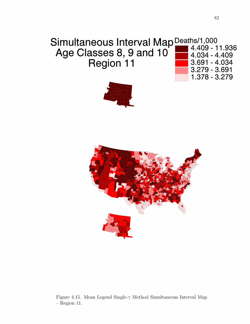
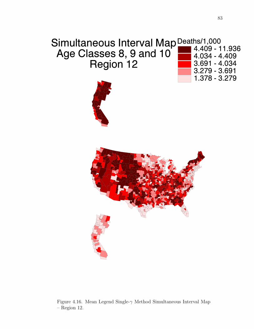
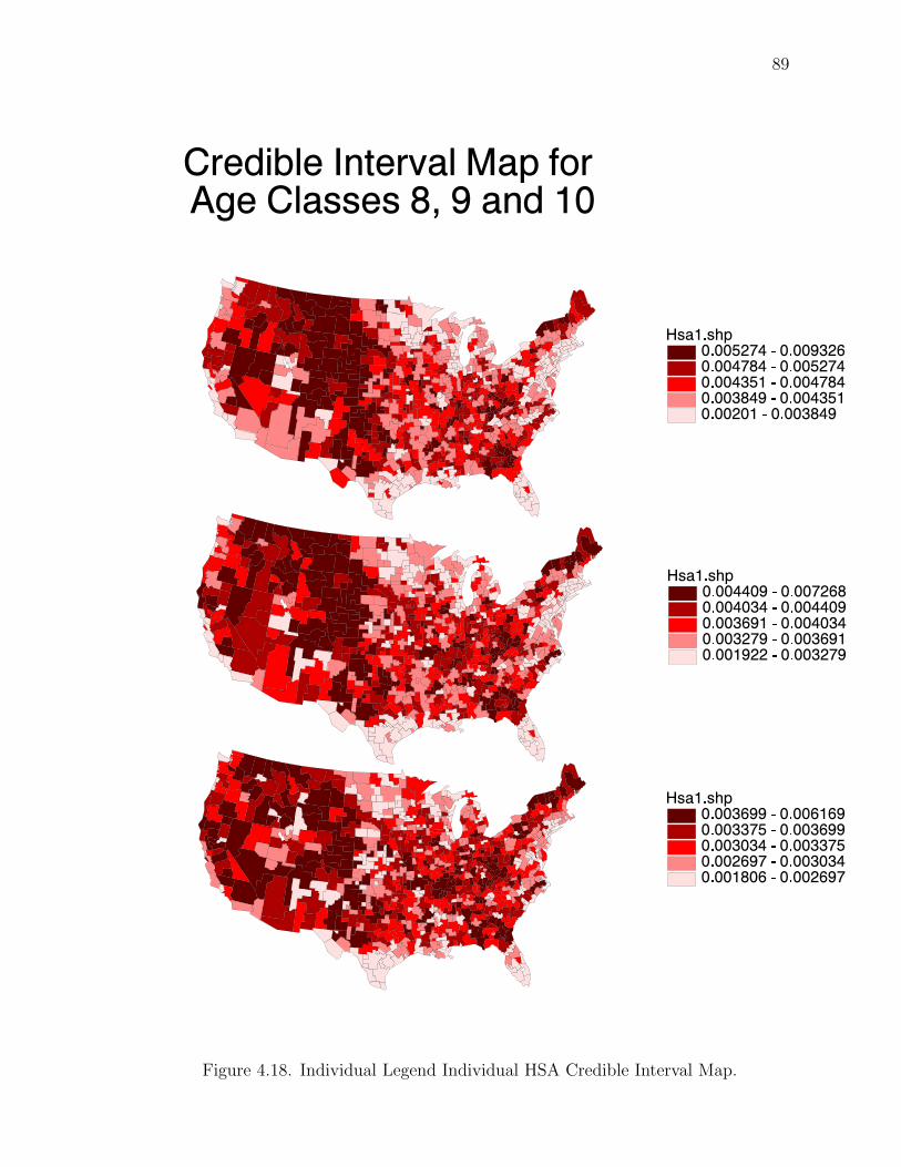
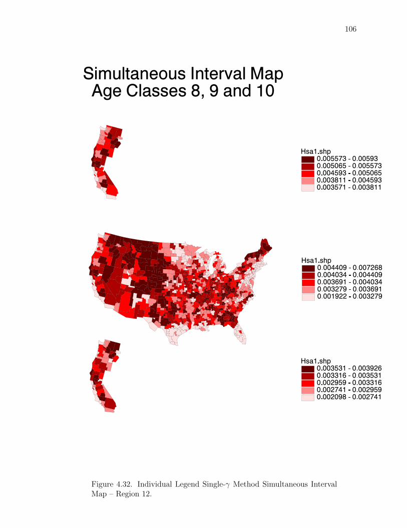
Figure 3.2. Population size and death counts for COPD White MalesAge Classes 8, 9 and 10.

39

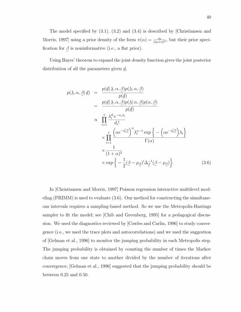
Letting λ˜ denote the vector of mortality rates, the joint density for the λi, given

α, β˜, is

π(λ˜|α, β˜) =∏i=1

(αe−x˜′iβ˜)α

λα−1i exp

−(αe−x˜′iβ˜)λi

Γ(α)

. (3.3)

(Note that x˜′iβ˜ = β0 + β1x1 + · · ·+ βp−1xp−1.)

The Poisson-Gamma model is an example of a famous result in Bayesian analysis,

namely that the posterior mean is a weighted average of the prior mean and the

sample mean. The details for our situation are given in Appendix B.2.

This model is attractive because of the conjugacy in which the conditional pos-

terior density of the λi is the simple gamma distribution. This permits us to con-

struct Rao-Blackwellized estimators of the λi. Such an estimator has smaller mean

square error than its empirical counterpart [Gelfand and Smith, 1990]. This makes

it convenient to construct the posterior simultaneous interval maps. In the standard

generalized linear model in which the log(λi) follow a normal linear model, it is not

possible to obtain simple Rao-Blackwellized estimators of the λi.

We take the shrinkage prior as the proper prior density for hyper-parameter α,

π(α) =1

(1 + α)2, α ≥ 0. (3.4)

One might prefer π(α) = a0

(a0+α)2, α ≥ 0, where a0 is the prior median of α, but we

have found that inference is nonsensitive to the choice of a0 (see [Albert, 1988] for

the choice of a0 = 1).

We take a multivariate normal density as the proper prior density for hyper-

parameters β˜,β˜ ∼ Normal

(µβ˜,∆β˜

)(3.5)

where µβ˜ and ∆β˜ are constants to be specified (∆β˜ includes variance inflation factor,

κv). We show how to specify µβ˜ and ∆β˜ using a weighted least squares analysis in

Appendix B.1.

40

The model specified by (3.1), (3.2) and (3.4) is described by [Christiansen and

Morris, 1997] using a prior density of the form π(α) = a0

(a0+α)2, but their prior speci-

fication for β˜ is noninformative (i.e., a flat prior).

Using Bayes’ theorem to expand the joint density function gives the joint posterior

distribution of all the parameters given d˜,

p(λ˜, α, β˜| d˜) =p(d˜|λ˜, α, β˜)p(λ˜, α, β˜)

p(d˜)=

p(d˜|λ˜, α, β˜)p(λ˜|α, β˜)p(α, β˜)p(d˜)

∝∏i=1

λdii e

−niλi

di!

×∏i=1


λα−1i exp


Γ(α)

× 1

(1 + α)2

× exp− 1

2(β˜ − µβ˜)′∆−1

β˜ (β˜ − µβ˜). (3.6)

In [Christiansen and Morris, 1997] Poisson regression interactive multilevel mod-

eling (PRIMM) is used to evaluate (3.6). Our method for constructing the simultane-

ous intervals requires a sampling-based method. So we use the Metropolis-Hastings

sampler to fit the model; see [Chib and Greenberg, 1995] for a pedagogical discus-

sion. We used the diagnostics reviewed by [Cowles and Carlin, 1996] to study conver-

gence (i.e., we used the trace plots and autocorrelations) and we used the suggestion

of [Gelman et al., 1996] to monitor the jumping probability in each Metropolis step.

The jumping probability is obtained by counting the number of times the Markov

chain moves from one state to another divided by the number of iterations after

convergence; [Gelman et al., 1996] suggested that the jumping probability should be

between 0.25 and 0.50.

41

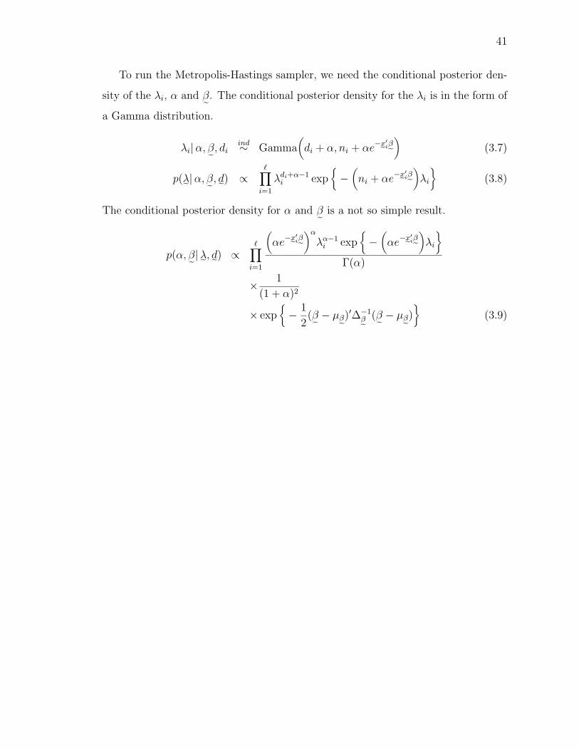
To run the Metropolis-Hastings sampler, we need the conditional posterior den-

sity of the λi, α and β˜. The conditional posterior density for the λi is in the form of

a Gamma distribution.

λi|α, β˜, diind∼ Gamma

(di + α, ni + αe−x˜′iβ˜) (3.7)

p(λ˜|α, β˜, d˜) ∝∏i=1

λdi+α−1i exp

−(ni + αe−x˜′iβ˜)λi

(3.8)

The conditional posterior density for α and β˜ is a not so simple result.

p(α, β˜|λ˜, d˜) ∝∏i=1


λα−1i exp


Γ(α)

× 1

(1 + α)2

× exp− 1

2(β˜ − µβ˜)′∆−1

β˜ (β˜ − µβ˜)

(3.9)

42

3.2 Computation using Markov chain Monte Carlo

With the model defined we proceed using Markov chain Monte Carlo (MCMC)

to make inference about the parameters of interest in the model, namely the rate

parameter λ˜. (Refer to Section A.3 for general information about Bayesian compu-

tational methods.) The particular MCMC method (see Section A.3.5) used here is

the Metropolis-Hastings sampler (see Section A.3.6). It works by drawing samples

from the conditional distributions. After a large number of iterations, the sample

converges to the joint posterior distribution.

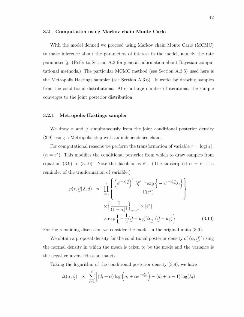
3.2.1 Metropolis-Hastings sampler

We draw α and β˜ simultaneously from the joint conditional posterior density

(3.9) using a Metropolis step with an independence chain.

For computational reasons we perform the transformation of variable τ = log(α),

(α = eτ ). This modifies the conditional posterior from which to draw samples from

equation (3.9) to (3.10). Note the Jacobian is eτ . (The subscripted α = eτ is a

reminder of the tranformation of variable.)

p(τ, β˜|λ˜, d˜) ∝∏i=1

(eτ−x˜′iβ˜)eτ

λeτ−1i exp

− eτ−x˜′iβ˜λi

Γ(eτ )

×

1

(1 + α)2

α=eτ

× |eτ |

× exp− 1

2(β˜ − µβ˜)′∆−1

β˜ (β˜ − µβ˜)

(3.10)

For the remaining discussion we consider the model in the original units (3.9).

We obtain a proposal density for the conditional posterior density of (α, β˜)′ using

the normal density in which the mean is taken to be the mode and the variance is

the negative inverse Hessian matrix.

Taking the logarithm of the conditional posterior density (3.9), we have

∆(α, β˜) ∝∑i=1

[(di + α) log

(ni + αe−x˜′iβ˜)+ (di + α− 1) log(λi)

43

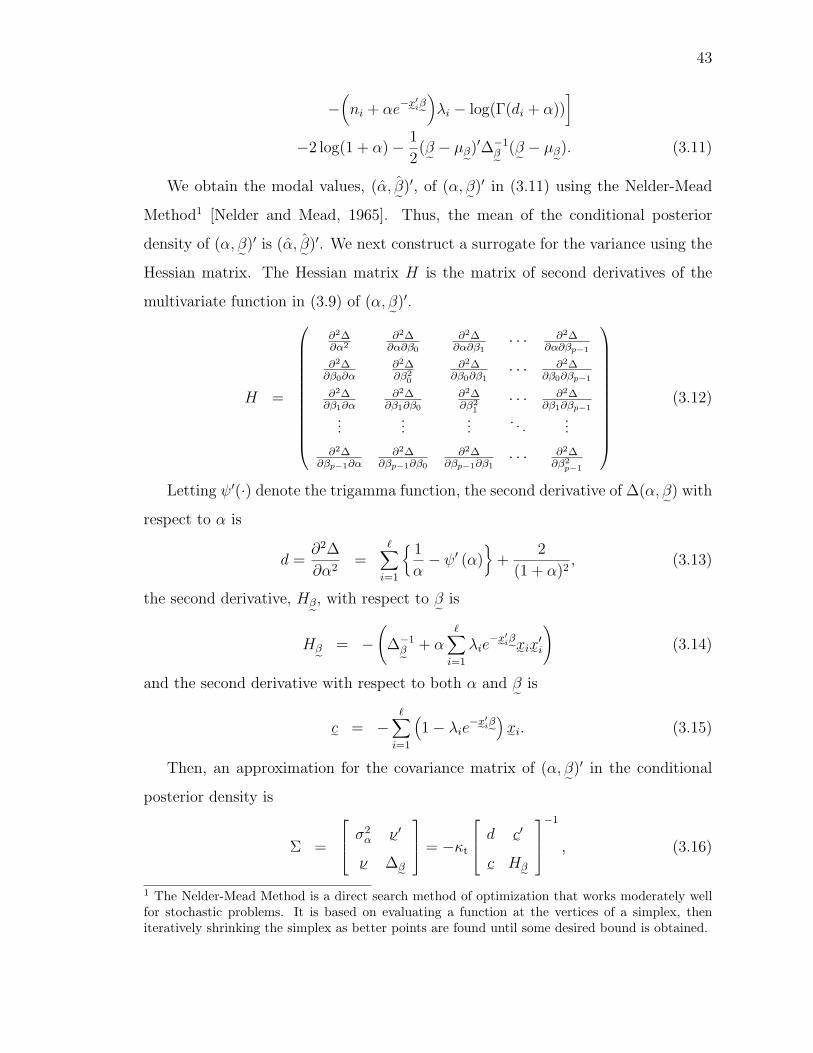
−(ni + αe−x˜′iβ˜)λi − log(Γ(di + α))

]−2 log(1 + α)− 1

2(β˜ − µβ˜)′∆−1

β˜ (β˜ − µβ˜). (3.11)

We obtain the modal values, (α, β˜)′, of (α, β˜)′ in (3.11) using the Nelder-Mead

Method1 [Nelder and Mead, 1965]. Thus, the mean of the conditional posterior

density of (α, β˜)′ is (α, β˜)′. We next construct a surrogate for the variance using the

Hessian matrix. The Hessian matrix H is the matrix of second derivatives of the

multivariate function in (3.9) of (α, β˜)′.

H =

∂2∆∂α2

∂2∆∂α∂β0

∂2∆∂α∂β1

· · · ∂2∆∂α∂βp−1

∂2∆∂β0∂α

∂2∆∂β2

0

∂2∆∂β0∂β1

· · · ∂2∆∂β0∂βp−1

∂2∆∂β1∂α

∂2∆∂β1∂β0

∂2∆∂β2

1· · · ∂2∆

∂β1∂βp−1

......

.... . .

...

∂2∆∂βp−1∂α

∂2∆∂βp−1∂β0

∂2∆∂βp−1∂β1

· · · ∂2∆∂β2

p−1

(3.12)

Letting ψ′(·) denote the trigamma function, the second derivative of ∆(α, β˜) with

respect to α is

d =∂2∆

∂α2=

∑i=1

1

α− ψ′ (α)

+

2

(1 + α)2, (3.13)

the second derivative, Hβ˜, with respect to β˜ is

Hβ˜ = −(

∆−1β˜ + α

∑i=1

λie−x˜′iβ˜x˜ix˜′i

)(3.14)

and the second derivative with respect to both α and β˜ is

c˜ = −∑i=1

(1− λie

−x˜′iβ˜) x˜i. (3.15)

Then, an approximation for the covariance matrix of (α, β˜)′ in the conditional

posterior density is

Σ =

σ2α ν˜′ν˜ ∆β˜

= −κt

d c˜′c˜ Hβ˜

−1

, (3.16)

1 The Nelder-Mead Method is a direct search method of optimization that works moderately wellfor stochastic problems. It is based on evaluating a function at the vertices of a simplex, theniteratively shrinking the simplex as better points are found until some desired bound is obtained.

44

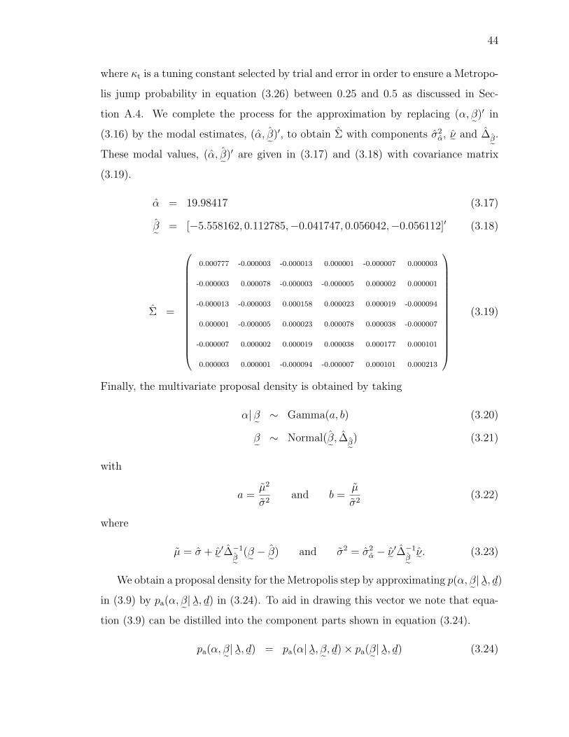
where κt is a tuning constant selected by trial and error in order to ensure a Metropo-

lis jump probability in equation (3.26) between 0.25 and 0.5 as discussed in Sec-

tion A.4. We complete the process for the approximation by replacing (α, β˜)′ in

(3.16) by the modal estimates, (α, β˜)′, to obtain Σ with components σ2α, ν˜ and ∆β˜.

These modal values, (α, β˜)′ are given in (3.17) and (3.18) with covariance matrix

(3.19).

α = 19.98417 (3.17)

β˜ = [−5.558162, 0.112785,−0.041747, 0.056042,−0.056112]′ (3.18)

Σ =

0.000777 -0.000003 -0.000013 0.000001 -0.000007 0.000003

-0.000003 0.000078 -0.000003 -0.000005 0.000002 0.000001

-0.000013 -0.000003 0.000158 0.000023 0.000019 -0.000094

0.000001 -0.000005 0.000023 0.000078 0.000038 -0.000007

-0.000007 0.000002 0.000019 0.000038 0.000177 0.000101

0.000003 0.000001 -0.000094 -0.000007 0.000101 0.000213

(3.19)

Finally, the multivariate proposal density is obtained by taking

α| β˜ ∼ Gamma(a, b) (3.20)

β˜ ∼ Normal(β˜, ∆β˜) (3.21)

with

a =µ2

σ2and b =

µ

σ2(3.22)

where

µ = σ + ν˜′∆−1

β˜ (β˜ − β˜) and σ2 = σ2α − ν˜′∆−1

β˜ ν˜. (3.23)

We obtain a proposal density for the Metropolis step by approximating p(α, β˜|λ˜, d˜)in (3.9) by pa(α, β˜|λ˜, d˜) in (3.24). To aid in drawing this vector we note that equa-

tion (3.9) can be distilled into the component parts shown in equation (3.24).

pa(α, β˜|λ˜, d˜) = pa(α|λ˜, β˜, d˜)× pa(β˜|λ˜, d˜) (3.24)

45

When we have a distribution we wish to generate, it may be easier, or save computa-

tion time, if we break it into pieces. This is called the composition method [Tanner,

1993]. For example, to draw (x, y) from f(x, y) = f(x| y)f(y), the composition

method draws y first from f(y), and then with this y, x is drawn from f(x| y). The

first distribution pa(α|λ˜, β˜, d˜) is Gamma while the second distribution pa(β˜|λ˜, d˜) is

Multivariate Normal given by realizations of (3.20) and (3.21).

First, a vector of β˜ deviates is drawn from the Multivariate Normal distribution

in equation (3.21). Next, a deviate of α is drawn from the Gamma distribution in

equation (3.20).

The Metropolis acception/rejection criterion is described in Section A.3.6. The

Metropolis ratio is defined as ψ(α, β˜) in equation (3.25) which is the ratio of equa-

tion (3.9) by equation (3.24). The probability of accepting the current proposal

density j and transitioning from the previous density i, or the jumping probability,

is given by equation (3.26).

ψ(α, β˜) =p(α, β˜|λ˜, d˜)pa(α, β˜|λ˜, d˜)

(3.25)

αij = min

ψ(α(j), β˜(j))

ψ(α(i), β˜(i)), 1

(3.26)

3.2.2 Sampling

To compute our maps, we first need a random sample from the joint posterior

density of Ω = (α, β˜). We obtain a random sample Ω(h), h = 1, . . . ,M (M = 10000),

from the Metropolis-Hastings sampler. We ran the Metropolis-Hastings sampler

for 101000 interations, using the first 1000 iterations as a “burn-in”. Then, we

picked every tenth interation from the remaining 100000 to make the autocorrelations

among the iterates negligible. A further check on the jumping rate of the Metropolis-

Hastings sampler shows the jumping probability is around 0.40 for all our activities.

Also, all the autocorrelations and numerical standard errors are small. Tuning of

46

the Metropolis step is obtained by varying the parameter κt in equation (3.16). We

found that κt = 1.3333 worked well.

3.2.3 Sampling Assessment

An assessment of the autocorrelations of the α and β˜ parameters show no signif-

icant correlation between iterations. This indicates they are from a random process.

Numerical standard error (NSE), or Monte Carlo error, using the batch means

method indicated high repeatibility because of the small standard error. As an

illustration of the batch means method, consider the NSE for the iterations of α.

Frist, average groups of iterates of a reasonable size (this paper uses groups of size

25 for 10,000 iterates), then take a grand average of the group averages.

x1 =1

25

25∑i=1

α(i)

x2 =1

25

50∑i=26

α(i)

...

x400 =1

25

10000∑i=9976

α(i)

¯x =1

400

400∑j=1

xj

NSE =

√√√√400∑i=1

(xi − ¯x)2/399

Also the acceptance rate in the Metropolis step was approximately 0.40, well

within the recommended range of 0.25 to 0.5.

We have specified the values of µβ˜ and ∆β˜ in our analysis, and therefore a sensi-

tivity analysis is relevant which has been studied through the variance inflation factor

κv by [Liu, 2002]. For various large values of κv [Liu, 2002] computed the averages

of the posterior mean and posterior standard deviation for the ` mortality rates. For

six values of κv from 10 to 100000, there were virtually no changes, indicating that

our method is robust to misspecification of these parameters and we can use almost

47

noninformative priors (see [Christiansen and Morris, 1997]) for a condition about

propriety of the posterior density, which is automatic in our model. In our empirical

work we set κv = 100000, which is almost a noninformative prior.

[Liu, 2002] also considered a measure, based on standardized cross-validation

residuals, to assess the fit of the model. Diagnositics described in [Nandram et al.,

1999] indicated the Poisson-gamma regression model provides a good fit to the COPD

mortality data for white males 65+.

Additionally, Table 3.2 gives the quantile values and 95% equal-tailed credible

interval from the 10,000 iterates of the α and β˜ parameters, and Table 3.3 gives the

means, standard deviations and confidence intervals for the mean.

48

Table 3.2Quantile values from 10,000 iterates of the α and β0 through β4 modelparameters.

Parameter Min 2.5% Q1 Q2 (Med) Q3 97.5% Max

α 18.8431 19.4798 19.7405 20.2008 21.1155 36.7517 74.2015

β0 -5.59958 -5.58038 -5.56819 -5.56290 -5.55684 -5.54356 -5.52273

β1 0.04480 0.08612 0.11136 0.12193 0.12961 0.14590 0.17974

β2 -0.08694 -0.06414 -0.05004 -0.04346 -0.03782 -0.02547 -0.00242

β3 0.00597 0.03446 0.05974 0.06774 0.07380 0.09504 0.13300

β4 -0.14360 -0.08792 -0.06798 -0.06144 -0.05161 -0.02537 0.02253

Table 3.3Sample summary for model parameters α and β0 through β4 from 10,000iterates.

Parameter Mean Std. Dev. 95% Confidence Interval

α 21.4771396 4.3199729 (21.3924595, 21.5618198)

β0 −5.5624099 0.0090993 (−5.5625883, −5.5622315)

β1 0.1197570 0.0147994 (0.1194669, 0.1200471)

β2 −0.0439811 0.0096623 (−0.0441705, −0.0437917)

β3 0.0666663 0.0138813 (0.0663942, 0.0669384)

β4 −0.0594216 0.0150388 (−0.0597164, −0.0591268)

49

3.3 Construction of the posterior interval maps

Our objective in this section is to show how to construct the maps of the posterior

mean and intervals described in Chapter 2 from the model described in Sections 3.1

and 3.2.

Note that the posterior density of λ˜ is

p(λ˜| d˜) =∫Ωp(λ˜| d˜,Ω)π(Ω| d˜) dΩ (3.27)

where Ω = (α, β˜) and the conditional posterior density of p(λ˜| d˜,Ω) is given by

equations (3.7) and (3.8). Equation (3.27) shows how we average over nuisance

parameters Ω to obtain the conditional posterior density of the parameter of interest

λ˜, given the observed data.

Here, Ω is a small p+1 dimensional vector, while λ˜ is the large ` = 798 dimensional

vector. As described in Section 3.2.1 we have a random sample λ˜(1), . . . , λ˜(M) from

p(λ˜| d˜).To determine the bounds of our intervals, we need to find two points (ai, bi)λi

that return the correct probability content, and satisfy a possible optimality criterion.

Note that it is impossible to obtain this result directly from p(λ˜| d˜) because we need

to integrate over the posterior density of Ω, π(Ω| d˜), which does not exist in closed

form. Therefore, we can not use standard analytical techniques such as calculus, but

use a numerical technique.

Below we first show how to construct the mean map, then resume discussing

interval maps.

50

3.3.1 Constructing the Mean Map

We construct the posterior mean map using Rao-Blackwellized estimators for the

λi. As in Section 3.1, letting ri = di/ni, i = 1, . . . , `, denote the observed mortality

rate and letting Λi = ni/(ni +αe−x˜′iβ˜), from (3.7) the expectation of the conditional

posterior mean of λi is

E(λi|α, β˜, di) = Λiri + (1− Λi)ex˜′iβ˜. (3.28)

As expected, this is a weighted average of the observed mortality rate and the prior

mortality rate (see Appendix B.2). It follows that the posterior mean (unconditional)

of λi is

µi = E(λi| d˜)= EΩ| di˜

Λiri + (1− Λi)e

x˜′iβ˜ . (3.29)

Note that because of the conditioning (posterior) on the data, µi is a function of the

data. The Rao-Blackwellized estimator of µi is

µi = M−1M∑

h=1

Λ

(h)i ri + (1− Λ

(h)i )ex˜′iβ˜(h)

(3.30)

where Λ(h)i = ni/(ni + α(h)e−x˜′iβ˜(h)

) and Ω(h) = (α(h), β˜(h)), h = 1, . . . ,M , are the

M iterates obtained from the Metropolis-Hastings sampler. Therefore, the iterates

of λi are λ(h)i = Λ

(h)i ri + (1 − Λ

(h)i )ex˜′iβ˜(h)

. The posterior mean map is obtained by

mapping the µi in (3.30) for all ` = 798 HSAs. See Section 4.1.1 for the resulting

map from this process.

51

3.3.2 Constructing the Credible Interval Map

The method for constructing the posterior credible interval map follows automat-

ically from the output of the Metropolis-Hastings sampler already described. First,

perform a sort on each set λ(1)i , . . . , λ

(M)i , i = 1, . . . , `, giving λ

(1∗)i , . . . , λ

(M∗)i . Next,

choose from these the α2

and 1 − α2

quantiles (see Section 2.1.1); for α = 0.05 and

M = 10000, we choose the 2.5 and 97.5 quantiles, or λ(250∗)i and λ

(9751∗)i . Thus the

problem simply reduces to sorting and extracting the desired quantiles for each HSA.

See Section 4.1.2 for the resulting map from this process.

52

3.3.3 Constructing the HPD Interval Map

The method for constructing the posterior HPD interval Map is computationally

intensive, but it follows easily from the output of the Metropolis-Hastings sampler

already described. Our procedure calculates ordinates p(λi| di) at each of the points

λ(1)i , . . . , λ

(M)i , i = 1, . . . , `. Therefore, we need to find lower and upper bounds ai

and bi, on the support of λi, such that both conditions in equations (3.31), content,

and (3.32), equal ordinates, are satisified (see Section 2.1.2).

∫ bi

ai

p(λi| di) dλi = 1− α (3.31)

p(ai| di) = p(bi| di) (3.32)

Using the output of the Metropolis-Hastings sampler, we approximate the content

in equation (3.31) by

1− α =∫Ω

∫ bi

ai

p(λi| di,Ω)π(Ω| di) dλi dΩ

=∫ΩF (bi| di,Ω)− F (ai| di,Ω) π(Ω| di) dΩ

≈ M−1M∑

h=1

F (bi| di,Ω

(h))− F (ai| di,Ω(h))

(3.33)

where F (·) is the cdf and we approximate the ordinates in equation (3.32) for ai by

p(ai| di,Ω) =∫Ωp(ai| di,Ω)π(Ω| di) dΩ

≈ M−1M∑

h=1

p(ai| di,Ω(h)) (3.34)

and for bi by

p(bi| di,Ω) =∫Ωp(bi| di,Ω)π(Ω| di) dΩ

≈ M−1M∑

h=1

p(bi| di,Ω(h)). (3.35)

For the simultaneous solution to both these non-linear equations we use the

Nelder-Mead Method to minimize a function composed from (3.33), (3.34) and (3.35).

We use the results from the credible interval in Section 3.3.2 as starts for ai and bi

53

in the minimization routine. Function f(ai, bi) in equation (3.36) is minimized over

parameters ai and bi. The minimum value of the fuction f(ai, bi) occurs at the same

point where f(ai, bi) = 0 (i.e., each term in equation (3.36) is 0).

f(ai, bi) =

∣∣∣∣∣M−1M∑

h=1

F (bi| di,Ω

(h))− F (ai| di,Ω(h))

− (1− α)

∣∣∣∣∣+

∣∣∣∣∣M−1M∑

h=1

p(ai| di,Ω(h))−M−1

M∑h=1

p(bi| di,Ω(h))

∣∣∣∣∣ (3.36)

54

3.3.4 Constructing the Simultaneous Interval Map

The method for constructing the posterior simultaneous interval map is computa-

tionally intensive, but it follows easily from the output of the HPD Interval routine.

As described in Sections 2.4 and 2.5 we use parameter γ as a “stretching” factor on

the HPD intervals (ai, bi), i = 1, . . . , `, to produce the desired simultaneous proba-

bility content. For the Single-γ Method, 0 < γ < 1 is used to obtain the content;

for the Double-γ Method, 0 < γ1 < 1 and 0 < γ2 < 1 are used to obtain the content

and satisfy an equal ordinates optimality criterion.

3.3.5 Single-γ Method

We need to find the value of γ in the lower and upper bounds γai and bi/γ such

that the probability content in equation (3.37) is satisified. Using the output of

the Metropolis-Hastings sampler, we approximate the integral in equation (3.37) by

(3.39).

1− α =∫Ω

∫ b`/γ

γa`

· · ·∫ b1/γ

γa1

p(λ1| d1,Ω) · · · p(λ`| d`,Ω)π(Ω| d˜)dλ1 · · · dλ` dΩ (3.37)

=∫Ω

∏i=1

F (bi/γ| di,Ω)− F (γai| di,Ω) π(Ω| di) dΩ (3.38)

≈ M−1M∑

h=1

[∏i=1

F (bi/γ| di,Ω

(h))− F (γai| di,Ω(h))

]. (3.39)

For the solution to this non-linear equation we use the Nelder-Mead Method

to minimize a function composed from (3.39). Function f(γ) in equation (3.40) is

minimized over parameter γ. The minimum value of this function is clearly zero.

f(γ) =

∣∣∣∣∣M−1M∑

h=1

[∏i=1

F (bi/γ| di,Ω

(h))− F (γai| di,Ω(h))

]− (1− α)

∣∣∣∣∣ (3.40)

55

3.3.6 Double-γ Method

We need to find the values of γ1 and γ2 in the lower and upper bounds γ1ai and

bi/γ2 such that both conditions of content, in equation (3.41), and equal ordinates,

S∗o (see Section 2.6), are satisified. Using the output of the Metropolis-Hastings

sampler, we approximate the integral in equation (3.41) by (3.43).

1− α =∫Ω

∫ b`/γ2

γ1a`

· · ·∫ b1/γ2

γ1a1

p(λ1| d1,Ω) · · · p(λ`| d`,Ω)π(Ω| d˜)dλ1 · · · dλ` dΩ (3.41)

=∫Ω

∏i=1

F (bi/γ2| di,Ω)− F (γ1ai| di,Ω) π(Ω| di) dΩ (3.42)

≈ M−1M∑

h=1

[∏i=1

F (bi/γ2| di,Ω

(h))− F (γ1ai| di,Ω(h))

]. (3.43)

For the solution to this non-linear equation we use the Nelder-Mead Method to

minimize a function composed from (3.43) and optimality criterion S∗o . Function

f(γ1, γ2) in equation (3.44) is minimized over parameters γ1 and γ2. The minimum

value of this function is clearly zero.

f(γ1, γ2) =

∣∣∣∣∣M−1M∑

h=1

[∏i=1

F (bi/γ2| di,Ω

(h))− F (γ1ai| di,Ω(h))

]− (1− α)

∣∣∣∣∣+|S∗o | (3.44)

3.3.7 Equal Ordinate condition optimization criterion

The computational aspects of those methods described in Section 2.6 are pro-

vided below. Because these are calculated numerically, they are dependent upon M

samples from a MCMC simulation.

3.3.8 Maximum Relative Difference Criterion

To calculate the Maximum Relative Difference, evaluate the ordinates over the

M iterates for each of the ` areas. Individually average the left and right ordinates

56

for each area and take the ratio of the larger average over the lesser average to obtain

the larger ratio. This ratio will be one when the ordinates are equal. Subtract one

from the ratio and take absolute value as a measure of the difference between these

ordinates. Finally, find the maximum value over all ` areas. Set this equal to S∗1 and

use in equation (3.44), where

S∗1 = maxi∈1,...,`

[∣∣∣∣∣max

M−1∑M

h=1 p(γ1ai| di,Ω(h))

M−1∑M

h=1 p(bi/γ2| di,Ω(h)),

M−1∑Mh=1 p(bi/γ2| di,Ω

(h))

M−1∑M

h=1 p(γ1ai| di,Ω(h))

− 1

∣∣∣∣∣]. (3.45)

3.3.9 Average Relative Difference Criterion

To calculate the Average Relative Difference, evaluate the ordinates for each of

the ` areas over the M iterates. Take the ratio of the absolute difference of the left

and right ordinates over their sum. This ratio will be zero when the ordinates are

equal. Average these over all ` areas. Finally, average over the M iterates. Set this

equal to S∗2 and use in equation (3.44), where

S∗2 =

`−1∑i=1

∣∣∣M−1∑Mh=1 p(γ1ai| di,Ω

(h))−M−1∑Mh=1 p(bi/γ2| di,Ω

(h))∣∣∣

M−1∑M

h=1 p(γ1ai| di,Ω(h)) +M−1∑M

h=1 p(bi/γ2| di,Ω(h))

.(3.46)

This method uses the ratio of the difference to the sum to adjust for possibly large

differences in ordinate magnitude between areas. This gives each area equal weight

in the optimization.

3.3.10 Average Absolute Difference Criterion

To calculate the Average Absolute Difference, evaluate the ordinates for each of

the ` areas over the M iterates. Take the absolute difference of the left and right

ordinates. This difference will be zero when the ordinates are equal. Average these

57

over all ` areas. Finally, average over the M iterates. Set this equal to S∗3 and use

in equation (3.44), where

S∗3 =

`−1

∑i=1

∣∣∣∣∣M−1M∑

h=1

p(γ1ai| di,Ω(h))−M−1

M∑h=1

p(bi/γ2| di,Ω(h))

∣∣∣∣∣. (3.47)

This method does not adjust for possibly large differences in ordinate magnitude

between areas. A few areas are likely to dominate this optimization.

58

59

4. MAPS AND ASSESSMENT

The following are the results from the individual and simultaneous interval methods

discussed in previous chapters. A variety of methods are used to present the re-

sults. We present two types of choropleth map: interval maps and difference maps.

Two types of interval maps are used. The first are mean legend maps, where the

interval maps use the common legend of the mean map. The second are individual

legend maps, where the interval maps use their own legend. These interval maps

are given for credible intervals (CI), highest posterior density intervals (HPD), and

simultaneous intervals. Simultaneous interval maps are given for regions considered

together (all) and seperately (regions 1 through 12). To accompany each of these

interval maps, difference maps are given in an attempt to capture the variation ob-

served between the lower and upper interval maps in terms of legend color difference.

Difference tables are provided as a further summary.

We first present the mean map, which is the map of the parameter estimates. The

mean map is then banded by a set of interval maps, an upper and a lower. The first

set of interval maps are mean legend maps: CI, HPD and simultaneous intervals.

Values for γ are given for the Single-γ Method and the simultaneous probability

content of the CI, HPD, Single-γ Method, and Besag intervals. The Single-γ Method

is the only method providing the correct probability content. Mean legend difference

maps and tables are then presented to help summarize the variation observed.

The second set of interval maps are individual legend maps: CI, HPD and simul-

taneous intervals. Individual legend difference maps and tables are then presented

to help summarize the variation observed.

Finally, values for γ1, γ2 are given for the Double-γ Method. In our case, the

Single-γ Method and Double-γ Method provide indistinguishable results, so no maps

are given for the Double-γ Method. Instead, tables to compare values for γ from

60

the Single-γ Method and γ1 and γ2 from the Double-γ Method are given. Also, to

compare the sensitivity of the simultaneous intervals on the prerequisite of HPD

intervals, we obtain the simultaneous intervals based on the credible intervals.

4.1 Mean Legend Choropleth Maps

The maps in this section are visualizations of the rate parameter, λ, for mortality

of White Males age classes 8, 9 and 10 (65 years and older) for each HSA given by

the fitted model in Section 3.1.

In the production and presentation of these maps several standards are adhered

to. All maps are colored with the same five-color monochromatic color scheme with

light representing a low rate and dark representing a high rate, allowing for gray-

scale transition (for non-color printing). The cutpoints of the legend colors are

based on the quintiles of the Mean map. All intervals maps are 95% intervals. In the

interval maps the map representing the upper bound is the upper map, and the map

representing the lower bound is the lower map. The mean map is always presented

between the upper and lower maps as a basis of reference. The legend bounds are

adjusted to reflect the maximum upper bound and minimum lower bound, but the

cutpoints remain the same for comparison. In the simultaneous interval maps by

region, only the region of interest is displayed in the upper and lower maps and they

differ only in the legend bounds. All the legend bounds are the maximum of all

the maximum bounds and the minimum of all the minimum bounds. These similar

legends saved hours of legend editing, and the individual bounds can be referenced

in Table 4.2.

To illustrate how one might use the interval maps presented, select an HSA from

the mean map. Find the corresponding HSA on both the upper and lower maps.

The variation of the particular HSA selected based on the quintiles of the mean map

can be interpreted from the colors and number of color differences from the lower to

the upper map. An HSA that changes one color or not at all can be said to have

61

little variation, except in the extreme colors, while an HSA that changes four colors

can be said to have great variation.

62

4.1.1 Mean Map

The plot in Figure 4.1 gives the mean map. These means are computed from the

model but also correspond with the observed rates.

Mean map minimum, maximum and quintile cutpoints are presented together

with the minimum of the lower and maximum of the upper maps for the credible

interval (Section 4.1.2) and HPD intervals maps (Section 4.1.3) in Table 4.1. Notice

that the HPD extremes are less than the CI extremes.

Table 4.1Mean map minimum, maximum and quintiles and CI and HPD mapminimum lower and maximum upper values

Map min Q1 Q2 Q3 Q4 maxMean 0.001922 0.003279 0.003691 0.004034 0.004409 0.007268

CI 0.001806 0.009326HPD 0.001788 0.009204

63

Figure 4.1. Mean Map.

64

4.1.2 Individual HSA Credible Interval Map

The plot in Figure 4.2 gives the individual HSA credible interval map. The

upper and lower maps are based on the equal tail credible intervals described in

Section 2.1.1.

65

Figure 4.2. Mean Legend Individual HSA Credible Interval Map.

66

4.1.3 Individual HSA HPD Interval Map

The plot in Figure 4.3 gives the individual HSA HPD interval map. The upper

and lower maps are based on the HPD intervals described in Section 2.1.2.

67

Figure 4.3. Mean Legend Individual HSA HPD Interval Map.

68

4.1.4 Single-γ Method Simultaneous Interval Map

The plot in Figure 4.4 gives the Single-γ Method simultaneous interval map.

The upper and lower maps are based on the Single-γ Method intervals described in

Section 2.4.

The value of γ for the various simultaneous maps in Sections 4.1.4 and 4.1.5

are given in Table 4.2. The value for γ is obtained by optimizing equation (2.17).

Column headers are Region and the corresponding region number, the number of

HSAs in the region (`), the optimum value for γ, and the map legend bounds as the

minimum of the lower map and the maximum of the upper map for the HSA rates

in the region. As expected, the value for γ is the smallest for when all regions are

considered with the general trend that it is larger when fewer HSAs are considered

simultaneously.

The simultaneous probability content is given in Table 4.3 (by taking the product

of the individual contents, or, for computational reasons, by exponentiating the sum

of the logs). The intervals are the Credible Interval (CI) from Section 3.3.2, Highest

Posterior Density Interval (HPD) from Section 3.3.3, Single-γ Method simultaneous

interval (SINT) from Section 3.3.4 each using 10000 iterates, and the NonParametric

Interval described by [Besag et al., 1995] from Appendix B.3 using 10000 iterates

(BESAG10) and 25000 iterates (BESAG25). The BESAG intervals are evaluated

against the Poisson-Gamma Hierarchical Regression Model for comparison. Obvious

details to note are the approximately zero simultaneous content for the CI and

HPD intervals for All regions, and the less than 0.15 simultaneous content for each

region. The Single-γ Method (SINT) is the only method that consistently obtains the

95% simultaneous coverage for all cases. BESAG10 underestimates and BESAG25

overestimates for All regions showing sensitivity to needing a large number of iterates;

10000 was too few for the correct content and 25000 shows the conservativity of the

method. For individual regions, BESAG25 is comparable to SINT.

69

Table 4.2Single-γ Method values for γ.

Region ` γ min(Lower) max(Upper)All All 798 0.7711593 0.001379 0.011935New England 1 23 0.9356322 0.002206 0.006979Middle Atlantic 2 49 0.9192618 0.001713 0.006132S. Atlantic-North 3 38 0.9109113 0.001852 0.007940S. Atlantic-South 4 88 0.8659650 0.001568 0.008893E. S. Central 5 88 0.8959517 0.002458 0.008035E. N. Central 6 121 0.8849109 0.002182 0.006640W. N. Central-North 7 45 0.8949770 0.002249 0.006502W. N. Central-South 8 105 0.8395072 0.001970 0.007899W. S. Central 9 115 0.8682747 0.001715 0.007171Mountain-South 10 40 0.8657598 0.001768 0.009689Mountain-North 11 38 0.8992667 0.003469 0.006927Pacific 12 48 0.9094602 0.002098 0.005930

Table 4.3Simultaneous Probability Content by Region for different methods.

Region ` CI HPD SINT BESAG10 BESAG25All 798 ≈ 10−18 ≈ 10−18 0.9500000559 0.8775405884 0.9867491722

1 23 0.3005571365 0.3073555529 0.9499999767 0.9450204968 0.94890236852 49 0.0811103284 0.0809937790 0.9500000607 0.9357133508 0.94227784873 38 0.1401147693 0.1423923075 0.9499999308 0.9497816563 0.94729775194 88 0.0109376954 0.0109569216 0.9500000762 0.9513514042 0.95643049485 88 0.0109985834 0.0109567912 0.9499999677 0.9328913093 0.94986146696 121 0.0019661339 0.0020162773 0.9500000947 0.9269511700 0.95373266947 45 0.0987905562 0.0994571149 0.9499999487 0.9302505851 0.93325436128 105 0.0045152325 0.0045811655 0.9499999014 0.9362568855 0.95204603679 115 0.0027406779 0.0027430130 0.9500000387 0.9310526848 0.9593409300

10 40 0.1266464740 0.1285093576 0.9500000617 0.9450564981 0.948727667311 38 0.1449352354 0.1424171031 0.9499999458 0.9326382875 0.934276640412 48 0.0858865231 0.0852592215 0.9500000411 0.9434457421 0.9476035237

70

Figure 4.4. Mean Legend Single-γ Method Simultaneous Interval Map.

71

4.1.5 Single-γ Method Simultaneous Interval by Region Maps

The plots in Figures 4.5 through 4.16 gives the Single-γ Method simultaneous

interval by region maps.

72

Figure 4.5. Mean Legend Single-γ Method Simultaneous Interval Map –Region 1.

73


74


75


76


77

Figure 4.10. Mean Legend Single-γ Method Simultaneous Interval Map– Region 6.

78


79


80


81


82


83


84

4.2 Mean Legend Difference Maps and Tables

A summary of the amount of variation observed in the maps can be described

in terms of the color difference from the low map to the high map based on the

quintiles of the Mean map. This comparison is in terms of only what is visible on

the map, namely, the color. The lightest color on the map representing the least rate

is indicated as 1 and the darkest color on the map representing the greatest rate is

indicated as 5. Difference maps and tables are presented below.

The plot in Figure 4.17 gives the Color Difference Maps for CI, HPD and All

Regions Simultaneous Maps. The colors given represent the change of color between

the low map and the high map. In our example the CI and HPD intervals are not

very different. However, because the HPD intervals are the narrowest intervals it is

expected that the color change map be slightly lighter in color than the CI maps.

Because of the fixed quintiles of the Mean Map, as the interval ends are adjusted

from the CI map to the HPD map, it is possible that one bound crosses a quintile

cut point so that the interval actually appears wider in terms of the colors. Because

our distributions are right skewed, the HPD intervals shift to lower values. Both the

left shift and the general trend of narrowing in the HPD can be seen in the tables

below.

Tables summarizing the difference maps are given in Table 4.4 for CI maps,

Table 4.5 for HPD maps and Table 4.6 for All Regions Simultaneous maps. As

an example of how to read these tables, consider cell (1, 1) in Table 4.4; 47 HSAs

are color 1 on the low map and color 1 on the high map, possibly indicating little

variation. Consider cell (3, 4); 5 HSAs are color 3 on the low map and color 4 on the

high map, also indicating little variation. Consider cell (1, 5); 160 HSAs are color

1 on the low map and color 5 on the high map, indicating the largest measurable

variation in terms of color.

85

Figure 4.17. Mean Legend Color Difference Maps for CI, HPD and AllRegions Simultaneous Maps.

86

Table 4.4Mean Legend Credible Interval difference between lower and upper boundmaps.

Lower Quintile Upper Quintile1 2 3 4 5

1 47 87 73 68 160 4352 0 0 10 44 144 1983 0 0 0 5 86 914 0 0 0 0 48 485 0 0 0 0 26 26

47 87 83 117 464 798

Table 4.5Mean Legend HPD Interval difference between lower and upper boundmaps.


1 48 88 74 77 155 4422 0 0 10 41 148 1993 0 0 0 5 82 874 0 0 0 0 45 455 0 0 0 0 25 25

48 88 84 123 455 798

Table 4.6Mean Legend Simultaneous Interval difference between lower and upperbound maps.


1 5 6 18 49 683 7612 0 0 0 0 30 303 0 0 0 0 4 44 0 0 0 0 1 15 0 0 0 0 2 2

5 6 18 49 720 798

87

4.3 Individual Legend Choropleth Maps

The maps presented in this section are the same as in Section 4.1, with one

difference; the cutpoints of each legend colors are based on the quintiles of each the

Upper, the Mean, and the Lower map. Therefore, each of the three maps has its

own legend based on the quintiles of that map.

To illustrate how one might use the interval maps presented, select an HSA from

the mean map. Find the corresponding HSA on both the upper and lower maps.

The variation of the particular HSA selected can be interpreted from the colors and

number of color differences from the lower to the upper map. An HSA that changes

from a dark color (in the lower) to a light color (in the upper) can be said to have

relatively little variation, while an HSA that changes from a light color (in the lower)

to a dark color (in the upper) can be said to have relatively great variation.

88

4.3.1 Individual Legend Individual HSA Credible Interval Map

The plot in Figure 4.18 gives the individual legend individual HSA credible in-

terval map. The upper and lower maps are based on the equal tail credible intervals

described in Section 2.1.1.

89

Figure 4.18. Individual Legend Individual HSA Credible Interval Map.

90

4.3.2 Individual Legend Individual HSA HPD Interval Map

The plot in Figure 4.19 gives the individual legend individual HSA HPD interval

map. The upper and lower maps are based on the HPD intervals described in

Section 2.1.2.

91

Figure 4.19. Individual Legend Individual HSA HPD Interval Map.

92

4.3.3 Individual Legend Single-γ Method Simultaneous Interval Map

The plot in Figure 4.20 gives the individual legend Single-γ Method simultaneous

interval map. The upper and lower maps are based on the Single-γ Method intervals

described in Section 2.4.

The value of γ for the various simultaneous maps in Sections 4.1.4 and 4.1.5 are

given in Table 4.2.

93

Figure 4.20. Individual Legend Single-γ Method Simultaneous IntervalMap.

94

4.3.4 Individual Legend Single-γ Method Simultaneous Interval by Re-

gion Maps

The plots in Figures 4.21 through 4.32 gives the Single-γ Method simultaneous

interval by region maps.

95

Figure 4.21. Individual Legend Single-γ Method Simultaneous IntervalMap – Region 1.

96


97


98


99


100


101


102


103


104


105


106


107

4.4 Individual Legend Difference Maps and Tables

A summary of the amount of variation observed in the maps can be described in

terms of the color difference from the low map to the high map. This comparison

is in terms of only what is visible on the map, namely, the color. The lightest color

on the map representing the least rate is indicated as 1 and the darkest color on

the map representing the greatest rate is indicated as 5. The difference presented

is the Lower map’s color number subtracted from the Upper map’s color number.

Difference maps and tables are presented below.

The plot in Figure 4.33 gives the Individual Legend Color Difference Maps for

CI, HPD and All Regions Simultaneous Maps. The colors given represent the change

of color between the low map and the high map.

Tables summarizing the difference maps are given in Table 4.7 for CI maps,

Table 4.8 for HPD maps and Table 4.9 for All Regions Simultaneous maps. As an

example of how to read these tables, consider cell (1, 1) in Table 4.7; 85 HSAs are

color 1 on the low map and color 1 on the high map, indicating moderate variation.

Consider cell (1, 4); 15 HSAs are color 1 on the low map and color 4 on the high

map, indicating high variation. Consider cell (5, 2); 29 HSAs are color 5 on the low

map and color 2 on the high map, indicating very little variation.

Tables summarizing the difference maps are given in Table 4.10 for All maps. As

an example of how to read these tables, consider row CI. There were 287 HSAs that

remained the same color between the lower and upper maps, 215 that were a shade

lighter in the upper map and 70 that were two shades darker in the upper map.

108

Figure 4.33. Individual Legend Color Difference Maps for CI, HPD andAll Regions Simultaneous Maps.

109

Figure 4.34. Individual Legend Color Difference Maps for SimultaneousMaps Regions 1, 2 and 3.

110


111


112


113

Table 4.7Individual Legend Credible Interval difference between lower and upperbound maps.


1 89 49 19 4 0 1612 37 40 53 29 0 1593 19 33 32 58 19 1614 13 22 27 41 55 1585 3 15 29 27 85 159

161 159 160 159 159 798

Table 4.8Individual Legend HPD Interval difference between lower and upperbound maps.


1 93 46 17 5 0 1612 34 43 55 27 0 1593 18 31 34 57 21 1614 12 22 28 40 56 1585 5 16 26 30 82 159

162 158 160 159 159 798

Table 4.9Individual Legend Simultaneous Interval difference between lower andupper bound maps.


1 93 46 17 5 0 1612 34 43 55 27 0 1593 18 31 34 57 21 1614 13 22 28 40 56 1595 4 16 26 30 82 158

162 158 160 159 159 798

114

Table 4.10Difference between individual legend lower and upper bound maps.

Method Reg -4 -3 -2 -1 0 1 2 3 4CI 3 28 70 124 287 215 67 4 0HPD 5 28 66 123 292 214 65 5 0SγM All 4 29 66 123 292 214 65 5 0SγM 1 0 0 0 2 19 2 0 0 0SγM 2 0 0 1 8 31 8 1 0 0SγM 3 0 0 2 4 25 6 1 0 0SγM 4 0 2 5 13 46 15 7 0 0SγM 5 0 0 5 18 44 14 6 1 0SγM 6 0 0 7 22 59 30 3 0 0SγM 7 0 0 0 10 26 8 1 0 0SγM 8 0 1 9 28 38 11 16 2 0SγM 9 0 0 3 29 54 23 6 0 0SγM 10 0 3 2 8 12 9 6 0 0SγM 11 0 0 1 8 19 10 0 0 0SγM 12 0 1 2 10 19 15 1 0 0

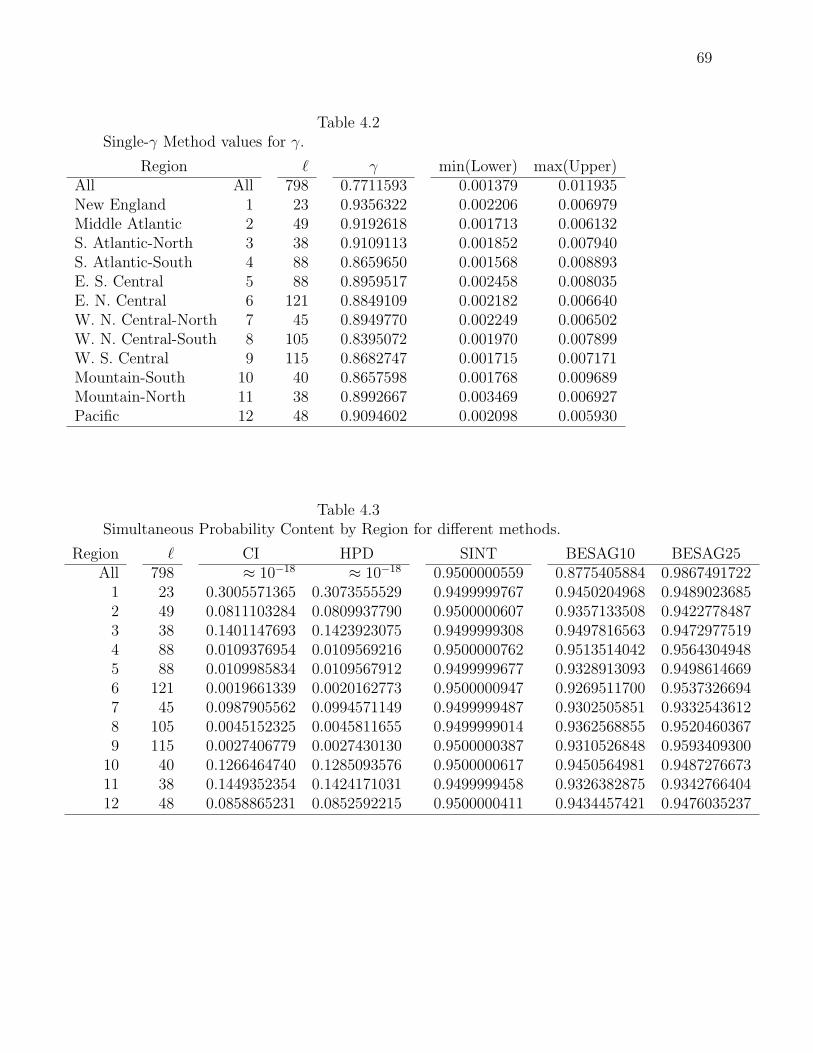
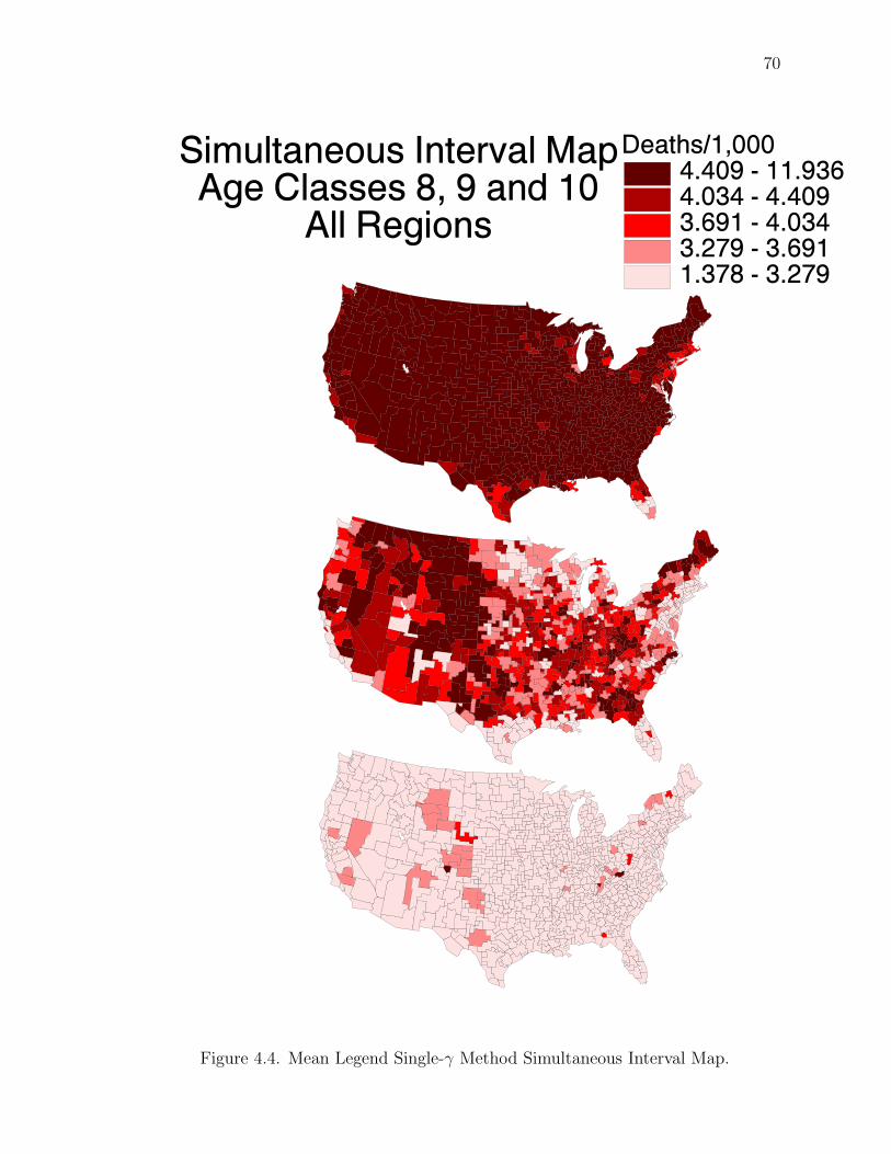
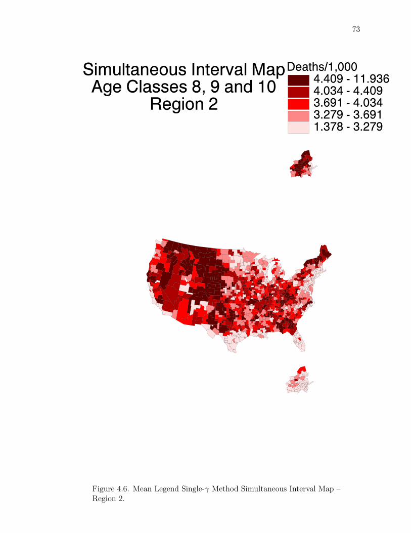
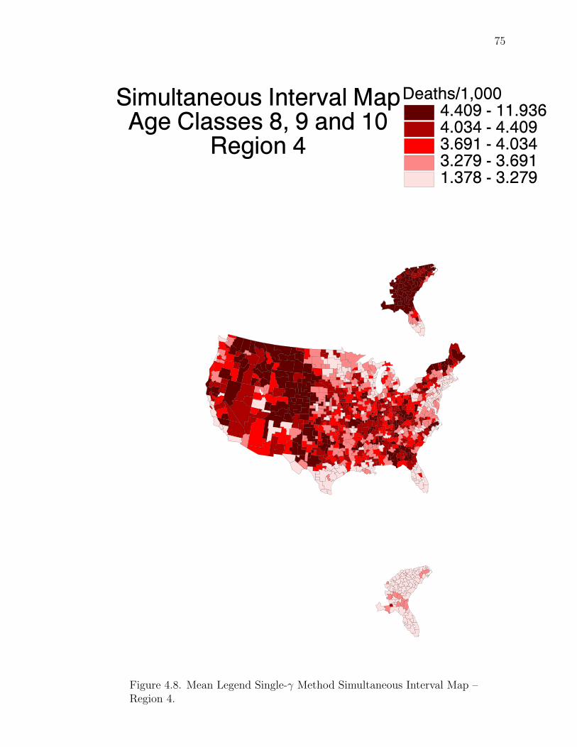
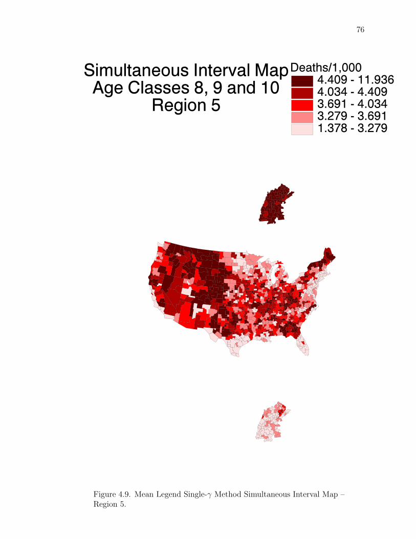
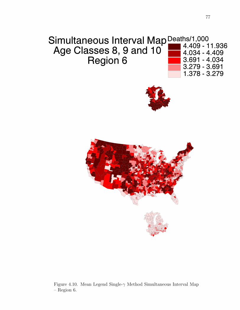
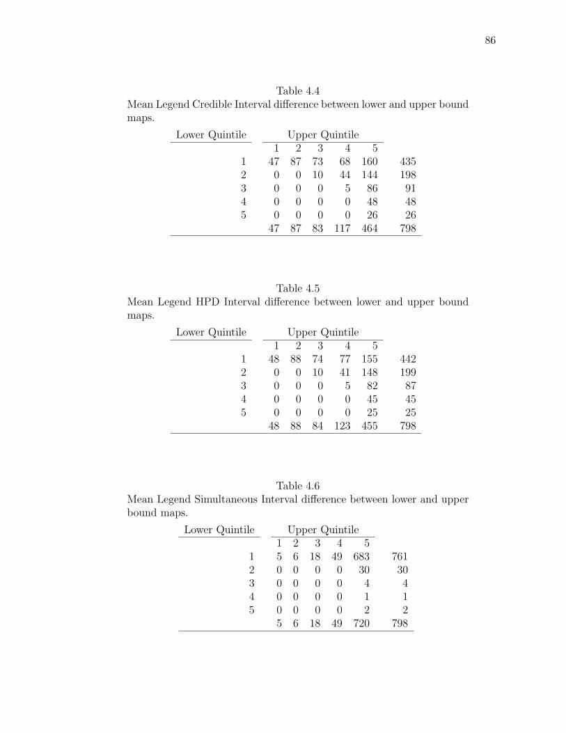
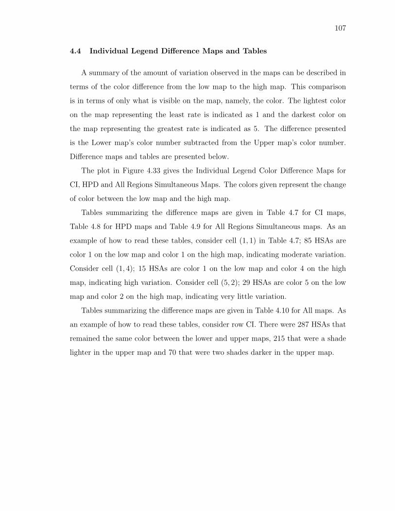
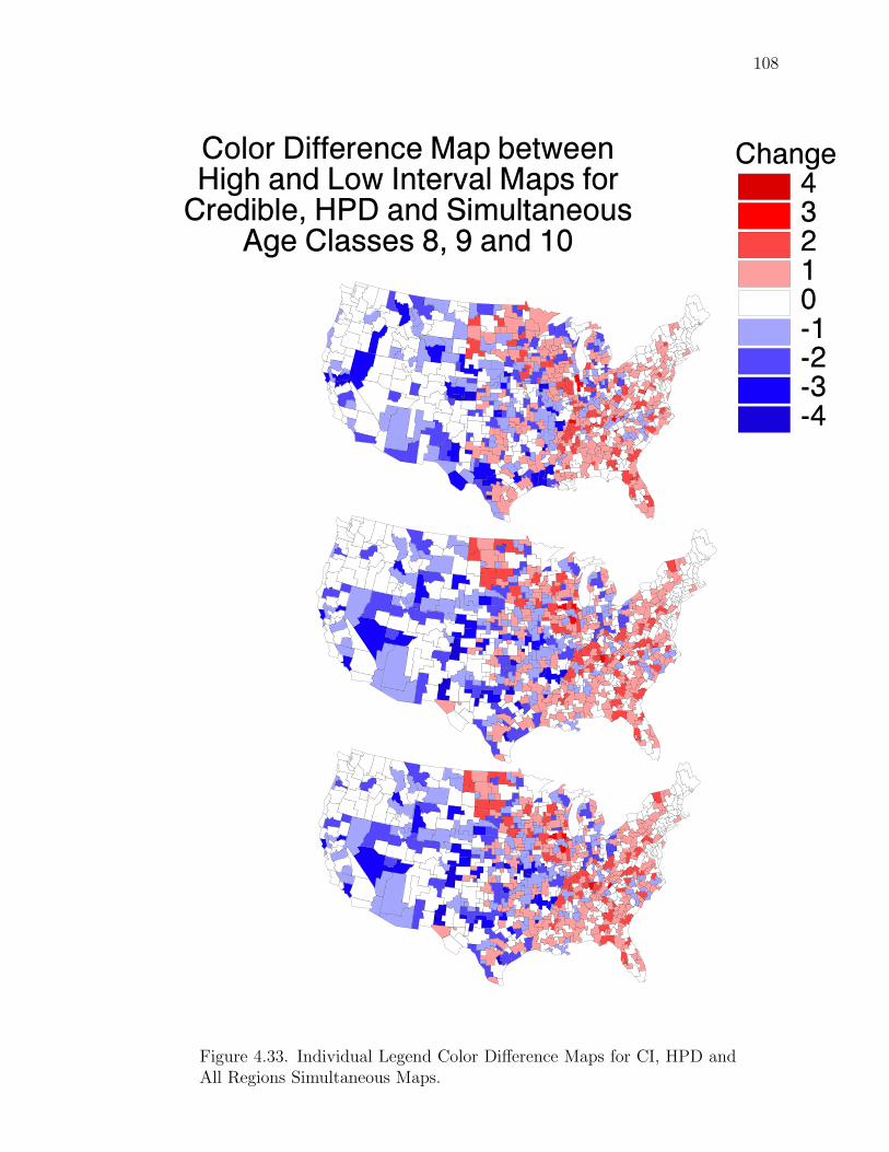
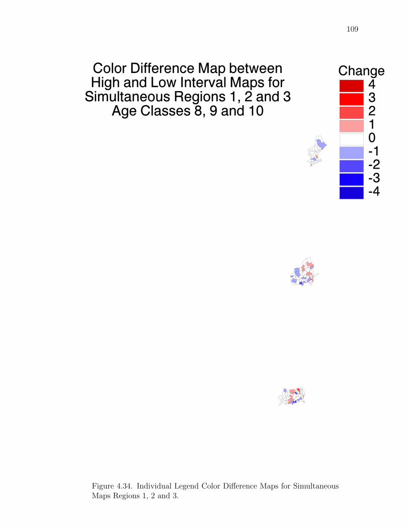
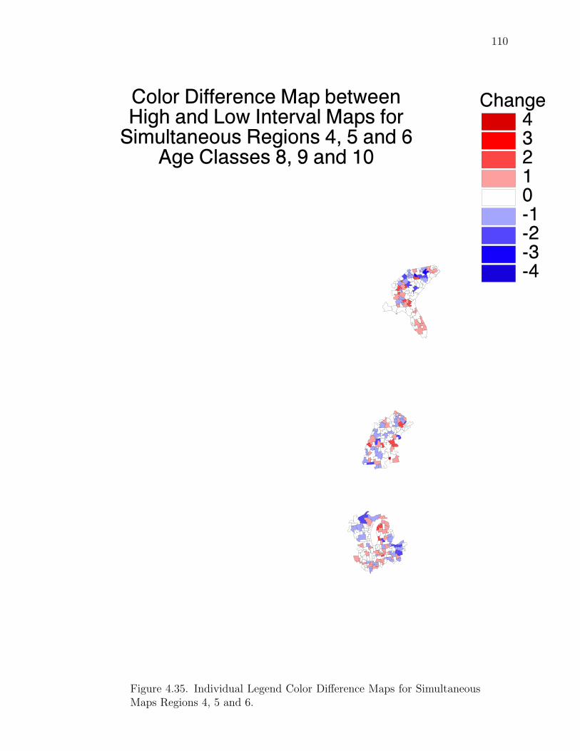
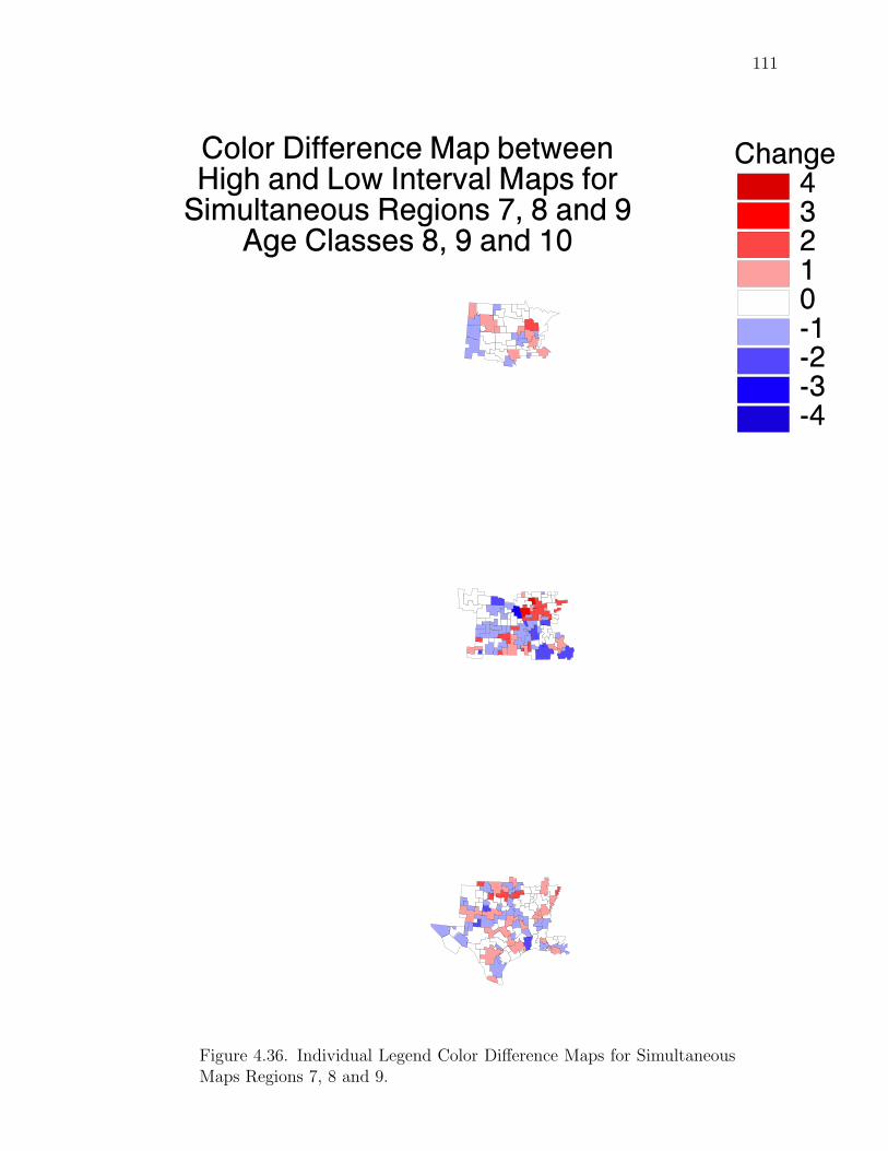
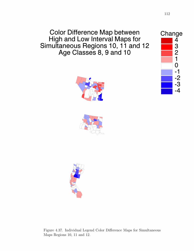
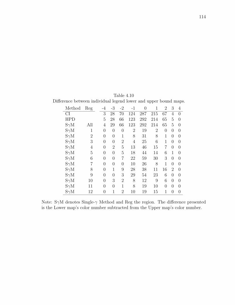
Note: SγM denotes Single-γ Method and Reg the region. The difference presentedis the Lower map’s color number subtracted from the Upper map’s color number.

115

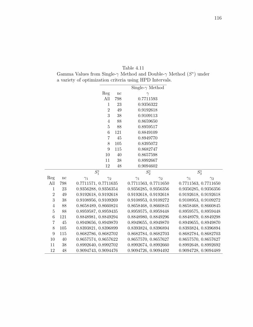
4.5 Double-γ Method Simultaneous Interval

Because Double-γ Method maps are virtually indistinguishable from Single-γ

Method maps, additional maps are not presented. Instead, we compare the value of

γ from the Single-γ Method with γ1 and γ2 from the Double-γ Method in Table 4.11.

As we expect, the value of γ (and γ1 and γ2) is generally smaller when more areas

are simultaneously considered.

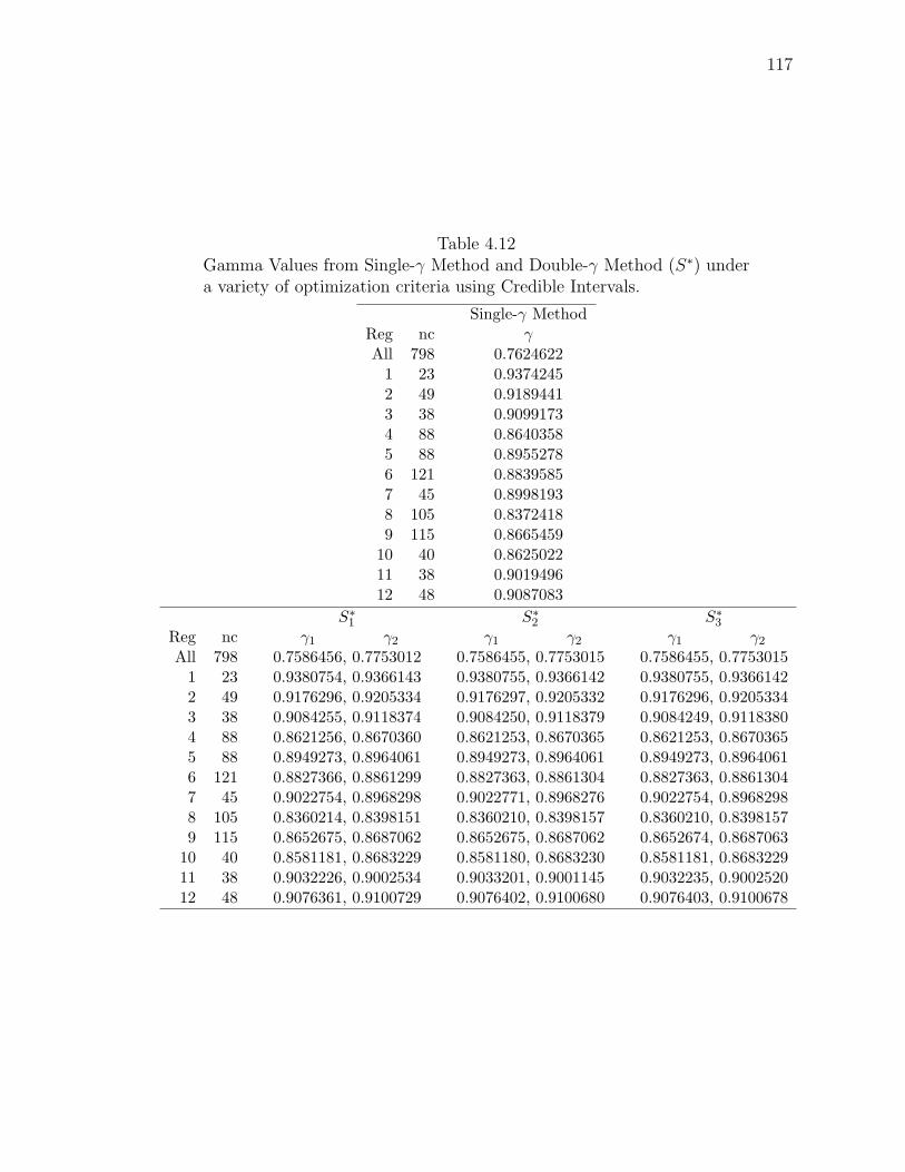
To compare the sensitivity of the simultaneous intervals on the prerequisite of

HPD intervals, we obtain the simultaneous intervals based on the credible intervals.

The γ and γ1 and γ2 values based on CIs are given in Table 4.12. To ease comparison,

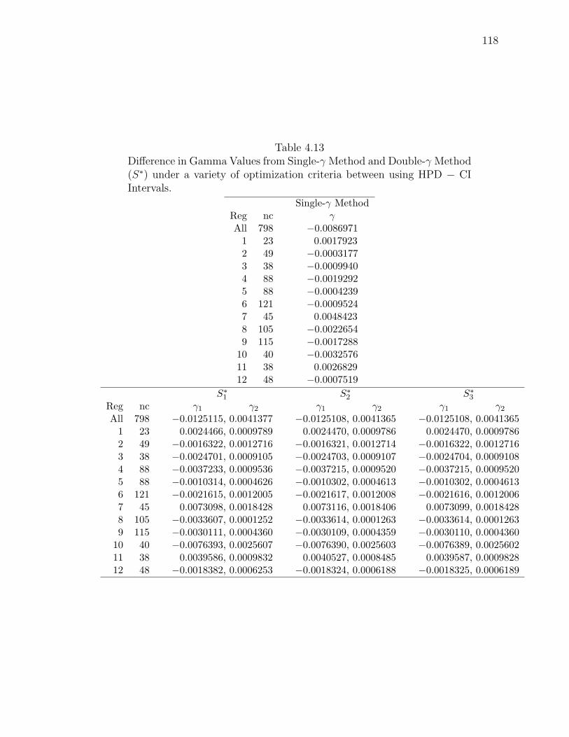
the difference of these values HPD − CI are given in Table 4.13.

We notice that there are differences between values of γ, γ1 and γ2 when starting

with credible intervals versus using HPD intervals. The difference is not large for the

Single-γ Method where no ordinate optimality criterion is specified. However, there

is a much larger difference for the Double-γ Method where the method compensates

when starting with the credible intervals of nonsymmetric densities to obtain equal

ordinates. This small difference is attributed to the symmetry of our individual

distributions. If the indiviual distributions are highly skewed, this difference will be

even greater.

116

Table 4.11Gamma Values from Single-γ Method and Double-γ Method (S∗) undera variety of optimization criteria using HPD Intervals.

Single-γ MethodReg nc γAll 798 0.7711593

1 23 0.93563222 49 0.91926183 38 0.91091134 88 0.86596505 88 0.89595176 121 0.88491097 45 0.89497708 105 0.83950729 115 0.8682747

10 40 0.865759811 38 0.899266712 48 0.9094602

S∗1 S∗2 S∗3Reg nc γ1 γ2 γ1 γ2 γ1 γ2

All 798 0.7711571, 0.7711635 0.7711563, 0.7711650 0.7711563, 0.77116501 23 0.9356288, 0.9356354 0.9356285, 0.9356356 0.9356285, 0.93563562 49 0.9192618, 0.9192618 0.9192618, 0.9192618 0.9192618, 0.91926183 38 0.9108956, 0.9109269 0.9108953, 0.9109272 0.9108953, 0.91092724 88 0.8658489, 0.8660824 0.8658468, 0.8660845 0.8658468, 0.86608455 88 0.8959587, 0.8959435 0.8959575, 0.8959448 0.8959575, 0.89594486 121 0.8848981, 0.8849294 0.8848980, 0.8849296 0.8848979, 0.88492987 45 0.8949656, 0.8949870 0.8949655, 0.8949870 0.8949655, 0.89498708 105 0.8393821, 0.8396899 0.8393824, 0.8396894 0.8393824, 0.83968949 115 0.8682786, 0.8682702 0.8682784, 0.8682703 0.8682784, 0.8682703

10 40 0.8657574, 0.8657622 0.8657570, 0.8657627 0.8657570, 0.865762711 38 0.8992640, 0.8992702 0.8992674, 0.8992660 0.8992648, 0.899269212 48 0.9094743, 0.9094476 0.9094726, 0.9094492 0.9094728, 0.9094489

117

Table 4.12Gamma Values from Single-γ Method and Double-γ Method (S∗) undera variety of optimization criteria using Credible Intervals.

Single-γ MethodReg nc γAll 798 0.7624622

1 23 0.93742452 49 0.91894413 38 0.90991734 88 0.86403585 88 0.89552786 121 0.88395857 45 0.89981938 105 0.83724189 115 0.8665459

10 40 0.862502211 38 0.901949612 48 0.9087083


All 798 0.7586456, 0.7753012 0.7586455, 0.7753015 0.7586455, 0.77530151 23 0.9380754, 0.9366143 0.9380755, 0.9366142 0.9380755, 0.93661422 49 0.9176296, 0.9205334 0.9176297, 0.9205332 0.9176296, 0.92053343 38 0.9084255, 0.9118374 0.9084250, 0.9118379 0.9084249, 0.91183804 88 0.8621256, 0.8670360 0.8621253, 0.8670365 0.8621253, 0.86703655 88 0.8949273, 0.8964061 0.8949273, 0.8964061 0.8949273, 0.89640616 121 0.8827366, 0.8861299 0.8827363, 0.8861304 0.8827363, 0.88613047 45 0.9022754, 0.8968298 0.9022771, 0.8968276 0.9022754, 0.89682988 105 0.8360214, 0.8398151 0.8360210, 0.8398157 0.8360210, 0.83981579 115 0.8652675, 0.8687062 0.8652675, 0.8687062 0.8652674, 0.8687063

10 40 0.8581181, 0.8683229 0.8581180, 0.8683230 0.8581181, 0.868322911 38 0.9032226, 0.9002534 0.9033201, 0.9001145 0.9032235, 0.900252012 48 0.9076361, 0.9100729 0.9076402, 0.9100680 0.9076403, 0.9100678

118

Table 4.13Difference in Gamma Values from Single-γ Method and Double-γ Method(S∗) under a variety of optimization criteria between using HPD − CIIntervals.

Single-γ MethodReg nc γAll 798 −0.0086971

1 23 0.00179232 49 −0.00031773 38 −0.00099404 88 −0.00192925 88 −0.00042396 121 −0.00095247 45 0.00484238 105 −0.00226549 115 −0.0017288

10 40 −0.003257611 38 0.002682912 48 −0.0007519


All 798 −0.0125115, 0.0041377 −0.0125108, 0.0041365 −0.0125108, 0.00413651 23 0.0024466, 0.0009789 0.0024470, 0.0009786 0.0024470, 0.00097862 49 −0.0016322, 0.0012716 −0.0016321, 0.0012714 −0.0016322, 0.00127163 38 −0.0024701, 0.0009105 −0.0024703, 0.0009107 −0.0024704, 0.00091084 88 −0.0037233, 0.0009536 −0.0037215, 0.0009520 −0.0037215, 0.00095205 88 −0.0010314, 0.0004626 −0.0010302, 0.0004613 −0.0010302, 0.00046136 121 −0.0021615, 0.0012005 −0.0021617, 0.0012008 −0.0021616, 0.00120067 45 0.0073098, 0.0018428 0.0073116, 0.0018406 0.0073099, 0.00184288 105 −0.0033607, 0.0001252 −0.0033614, 0.0001263 −0.0033614, 0.00012639 115 −0.0030111, 0.0004360 −0.0030109, 0.0004359 −0.0030110, 0.0004360

10 40 −0.0076393, 0.0025607 −0.0076390, 0.0025603 −0.0076389, 0.002560211 38 0.0039586, 0.0009832 0.0040527, 0.0008485 0.0039587, 0.000982812 48 −0.0018382, 0.0006253 −0.0018324, 0.0006188 −0.0018325, 0.0006189

119

5. CONCLUSION

In Chapter 1 we discussed choropleth maps and motivated the need for simultaneous

intervals in mapping applications. In Chapter 2 we discussed interval estimation, and

developed the Single-γ Method and Double-γ Method simultaneous intervals. We

have shown how to (a) find an exact content 100(1−α)% simultaneous interval having

a unique solution with a small number of parameters (one or two), and how to (b)

incorporate a variety of possible optimality criteria. In Chapter 3 we have shown how

to (c) fit the Poisson-gamma hierarchical regression model and how to (d) construct

intervals in this model context. Using an output analysis from the Metropolis-

Hastings sampler, we have shown how to (e) perform rate parameter estimation to

construct the mean map, and how to (f) construct simultaneous intervals to ensure

joint simultaneous coverage of 100(1− α)%. In Chapter 4 we presented results from

the simultaneous interval methods.

5.1 Accounting for map variation, epidemiological discussion

The model in Chapter 3 included a multiple linear regression to account for COPD

rate variation due to the four covariates in Table 3.1. Since the observed variation

is already adjusted for the covariates, what remains is unexplained variation. Areas

where relationship to covariates is not clear will have large variation.

We can examine the estimate variation unaccounted for by the covariates using

difference map in the third map in Figure 4.33 detailing the difference in quintile

between the lower and upper maps (upper−lower). The plot in Figure 5.1 (originally

from Section 4.3.3) gives the individual legend Single-γ Method simultaneous interval

map. Areas exhibiting the most variation are (3 color difference, there were none

that had 4) HSA 215 (Putnam, TN – Overton, TN), HSA 252 (Greene, TN – Cocke,

120

TN), HSA 338 (McLean (Bloomington), IL – De Witt, IL), HSA 361 (Clinton, IA –

Whiteside, IL) and HSA 373 (Kane (Aurora), IL – De Kalb, IL). Areas exhibiting

average variation include (0 color difference) HSA 3 (Sussex, DE – Wicomico, MD),

HSA 294 (Emmet, MI – Cheboygan, MI), HSA 565 (Ellis, KS – Graham, KS) and

HSA 816 (Inyo, CA – Mono, CA). Areas exhibiting the least variation are (−4 color

difference) HSA 513 (Bee, TX – Karnes, TX), HSA 518 (Howard, TX – Glasscock,

TX), HSA 704 (Pueblo (Pueblo), CO – Colfax, NM) and HSA 769 (Otero, NM –

Lincoln, NM).

5.2 Looking ahead

Another obvious factor effecting parameter variation is the size of the sample

(number of deaths in our case), a larger sample size contributing to a smaller vari-

ation. HSAs that exhibit variation either contrary or in excess of the sample size

effect are worth closer inspection. Accounting for this effect might be done within

the model itself, or as part of the output analysis.

Other interval “stretching” techniques can be considered to most preserve the

equal ordinate condition. Our Single-γ Method, (γa, b/γ), sends the left interval

bound a to zero at roughly the same rate as it sends the right interval bound b to

infinity while γ is close to one. However, the more the interval needs to be widened

to accommodate the desired probability content (γ close to zero), the further the

right bound is modified relative to the left bound. In our example we found similar

results for the Double-γ Method, (γ1a, b/γ2), which includes an ordinate optimization

criterion in order to maintain the equal ordinate condition.

Another equal ordinate condition optimization criterion to consider optimizes

over values of the pdf evaluated at the joint individual interval bounds. That is, for

` sets of interval bounds (ai, bi), i = 1, . . . , `, construct the 2` sets of joint interval

bounds with the objective of making the joint ordinates equal. These would be the

prefered ordinates to optimize rather than the individual ordinates.

121

Figure 5.1. Individual Legend Single-γ Method Simultaneous IntervalMap, recapitulation.

122

LIST OF REFERENCES

[Albert and Pepple, 1989] Albert, J. and Pepple, P. A. (1989). A bayesian approachto some overdispersion models. The Canadian Journal of Statistics, 17:333–344.

[Albert, 1988] Albert, J. H. (1988). Bayesian estimation methods for poisson meansusing hierarchical log linear model. In Bernardo, J. M., DeGroot, M. H., Lindley,D. V., and Smith, A. F. M., editors, Bayesian Statistics, volume 3. Proceedingsof the Third Valencia International Meeting on Bayesian Statistics. 519–531.

[Andrews and Birdsall, 1988] Andrews, R. W. and Birdsall, W. C. (1988). Simul-taneous confidence intervals: A comparison under complex sampling. In Designand Analysis of Repeated Surveys Section. Proceedings of the Survey ResearchMethods Section, American Statistical Association. 240–244.

[Aweh, 1999] Aweh, G. N. (1999). Bayesian analysis and mapping of breast cancermortality data for u.s. health service areas. Master’s thesis, Worcester PolytechnicInstitute, Worcester MA USA.

[Bates, 1989] Bates, D. V. (1989). Respiratory Function in Disease. Philadelphia:W. B. Saunders.

[Berger, 1990] Berger, J. O. (1990). Robust bayesian analysis – sensitivity to theprior. Journal of Statistical Planning and Inference, 25(3):303–328.

[Bernardinelli and Montomoli, 1992] Bernardinelli, L. and Montomoli, C. (1992).Empirical bayes versus fully bayesian analysis of geographical variation in diseaserisk. Statistics in Medicine, 11:983–1007.

[Bernardo et al., 1985] Bernardo, J. M., DeGroot, M. H., Lindley, D. V., and Smith,A. F. M., editors (1985). Generalized Linear Models: Parameters, Outliers Ac-commodation and Prior Distribution, volume 2. 531-558.

[Bernardo and Smith, 1994] Bernardo, J. M. and Smith, A. F. M. (1994). BayesianTheory. Chichester, UK: Wiley.

[Besag et al., 1995] Besag, J., Green, P., Higdon, D., and Mengersen, K. (1995).Bayesian computation and stochastic systems (with discussion). Statistical Sci-ence, 10:3–66.

[Besag et al., 1991] Besag, J., York, and Mollie, A. (1991). Bayesian image restora-tion with two applications in spatial statistics. Annals of the Institute of StatisticalMathematics, 43:1–59.

[Bonferroni, 1935] Bonferroni, C. E. (1935). Studi in Onore del Professore SalvatoreOrtu Carboni, chapter Il calcolo delle assicurazioni su gruppi di teste, pages 13–60.Rome: Italy.

123

[Bonferroni, 1936] Bonferroni, C. E. (1936). Teoria statistica delle classi e calcolodelle probabilita. Pubblicazioni del R Istituto Superiore di Scienze Economiche eCommerciali di Firenze, 8:3–62.

[Brooks and Roberts, 1998] Brooks, S. P. and Roberts, G. O. (1998). Assessingconvergence of markov chain monte carlo algorithms. Statistics and Computing,8(4):319–335.

[Chib and Greenberg, 1995] Chib, S. and Greenberg, E. (1995). Understanding themetropolis-hastings algorithm. The American Statistician, 49(4):327–335.

[Christiansen and Morris, 1997] Christiansen, C. L. and Morris, C. N. (1997). Hier-archical poisson regression modeling. Journal of the American Statistical Associ-ation, 92:618–632.

[Clayton and Kaldor, 1997] Clayton, D. G. and Kaldor, J. (1997). Empirical bayesestimates of age-standardized relative risks for use in disease mapping. Biometrics,43:671–681.

[Colon and Waller, 1998] Colon, E. and Waller, L. A. (1998). Flexible neighborhoodstructures in hierarchical models for disease mapping. Technical report, Universityof Minnesota.

[Connor and Morell, 1964] Connor, L. R. and Morell, A. J. H. (1964). Statistics inTheory and Practice. London: Pitman.

[Cowles and Carlin, 1996] Cowles, M. K. and Carlin, B. P. (1996). Markov chainmonte-carlo convergence diagnostics: a comparitive study. Journal of the Ameri-can Statistical Association, 91:883–904.

[Delcroix, 2000] Delcroix, S. M. (2000). Bayesian analysis of cancer mortality ratesfrom different types and their relative occurences. Master’s thesis, WorcesterPolytechnic Institute, Worcester MA USA.

[Duncan, 1952] Duncan, D. B. (1952). On the properties of the multiple comparisonstest. Virginia Journal of Science, 3:49–67.

[Efron, 1996] Efron, B. (1996). Double exponential families and their use in general-ized linear regression. Journal of the American Statistical Association, 81:709–721.

[English et al., 1999] English, P., Neutra, R., Scalf, R., Sullivan, M., Waller, L., andZhu, L. (1999). Examining associations between childhood asthma and trafficflow using a geographic information system. Environmental Health Perspectives,107:761–767.

[French and Smith, 1997] French, S. and Smith, J. Q. (1997). The Practice ofBayesian Analysis. London: Arnold.

[Gelfand and Smith, 1990] Gelfand, A. E. and Smith, A. F. M. (1990). Sampling-based approaches to calculating marginal densities. Journal of the American Sta-tistical Association, 85(410):398–409.

[Gelman et al., 1996] Gelman, A., Roberts, G. O., and Gilks, W. R. (1996).Bayesian Statitics, volume 5, chapter Efficient Metropolis jumping rules, pages599–607. Oxford University Press, New York.

124

[Gelman and Rubin, 1992] Gelman, A. and Rubin, D. B. (1992). Inference fromiterative simulation using multiple sequences (with discussion). Statistical Science,7:457–511.

[Hansen, 1991] Hansen, K. M. (1991). Head-banging: Robust smoothing in theplane. IEEE Transactions on Geoscienece and Remote Sensing, 29(3):369–378.

[Hastings, 1970] Hastings, W. K. (1970). Monte carlo sampling methods usingmarkov chains and their applications. Biometrika, 57:97–109.

[Jeffrey, 1961] Jeffrey, H. (1961). Theory of Probability, 3rd edition. Oxford: Claren-don Press.

[Kass and Steffey, 1989] Kass, R. E. and Steffey, D. (1989). Approximation bayesianinference in conditionally independent hierarchical models (parametric empiricalbayes models). Journal of the American Statistical Association, 84:717–726.

[Kleijnen, 1974] Kleijnen, J. P. C. (1974). Statistical Techniques in Simulation. NewYork: Marcel Dekker.

[Laird and Lewis, 1987] Laird, N. M. and Lewis, T. A. (1987). Empirical bayes con-fidence intervals based on bootstrap samples. Journal of the American StatisticianAssociation, 82:481–495.

[Lee, 1997] Lee, P. M. (1997). Bayesian Statistics: An Introduction, 2nd edition.London: Arnold.

[Lindley and Smith, 1972] Lindley, D. V. and Smith, A. F. M. (1972). Bayes es-timates for the linear model (with discussion). Journal of the Royal StatisticalSociety, B34:1–41.

[Liu, 2002] Liu, J. (2002). Novel bayesian methods for disease mapping: An ap-plication to chronic obstructive pulmonary disease. Master’s thesis, WorcesterPolytechnic Institute, Worcester MA USA.

[Lu and Morris, 1994] Lu, W. S. and Morris, C. N. (1994). Estimation in generalizedlinear empirical bayes model using the expected quasi-likelihood. Communicationsin Statistics, Part A – Theory and Methods, 23:661–688.

[Lui and Cumberland, 1987] Lui, K. J. and Cumberland, W. G. (1987). A bayesianapproach to small domain estimation. In Survey Research Method Section. Pro-ceedings of American Statistical Association. 347–352.

[McCullagh and Nelder, 1989] McCullagh, P. and Nelder, J. A. (1989). GeneralizedLinear Models. Chapman and Hall, London.

[Metropolis et al., 1953] Metropolis, N., Rosenbluth, A. W., Rosenbluth, M. N.,Teller, A. H., and Teller, E. (1953). Equations of state calculations by fast com-puting machines. Journal of Chemical Physics, 21:1087–1082.

[Miller, 1981] Miller, R. G. (1981). Simultaneous Statistical Inference. New York:Springer-Verlag.

[Mood et al., 1963] Mood, A., Graybill, F., and Boes, D. (1963). Introduction to theTheory of Statistics. New York: McGraw-Hill.

125

[Morgenthal, 1961] Morgenthal, G. W. (1961). The theory and application of sim-ulations in operations research. In Ackoff, R. L., editor, Progress in OperationsResearch. New York: Wiley.

[Morris and Munasinghe, 1994] Morris, R. D. and Munasinghe, R. L. (1994). Geo-graphic variability in hospital admission rates for respiratory disease among theelderly in the united states. Chest, 106:1172–1181.

[Mungiole et al., 1998] Mungiole, M., Pickle, L. W., and Simonson, K. H., editors(1998). Effects of Smoothing Mortality Data using the Weighted Head-BangingAlgorithm. American Statistical Association 1998 Meeting, Dallas, TX. 43-51.

[Mungiole et al., 1999] Mungiole, M., Pickle, L. W., and Simonson, K. H. (1999).Application of a weighted head-banging algorithm to mortality data maps. Statis-tics in Medicine, 18:3201–9.

[Murdoch and Green, 1998] Murdoch, D. J. and Green, P. J. (1998). Exact samplingfrom a continuous state space. Scandinavian Journal of Statistics, 25(3):483–502.

[Murdoch and Rosenthal, 1998] Murdoch, D. J. and Rosenthal, J. S. (1998). Regen-eration methods and exact sampling. In Sixth Valencia International Meeting onBayesian Statistics, Alcossebre, Spain. contributed paper.

[Nandram et al., 2003] Nandram, B., , Liu, J., and Choi, J. W. (2003). A comparisonof the posterior choropleth maps for disease mapping. Journal of Data Science,3(1).

[Nandram, 1993] Nandram, B. (1993). Bayesian cuboid prediction intervals: Anapplication to tensile-strength prediction. Journal of statistical planning and in-ference, 44:167–180.

[Nandram, 1998] Nandram, B. (1998). Generalized linear models: A Bayesian Per-spective, chapter Bayesian Generalized Linear Models for Inference about SmallAreas, by Balgobin Nandram. Marcel Dekker, New York.

[Nandram and Choi, 2003] Nandram, B. and Choi, J. W. (2003). Simultaneous con-centration bands for continuous random samples. Statistica Sinica, to appear.

[Nandram et al., 1999] Nandram, B., Sedrank, J., and Pickle, L. (1999). Bayesiananalysis of mortality rates for u.s. health service areas. Sankhya: The IndianJournal of Statistics, 61(Series B, Pt. 1):145–165.

[Nandram et al., 2000] Nandram, B., Sedransk, J., and Pickle, L. W. (2000).Bayesian analysis and mapping of mortality rates for chronic obstructive pul-monary disease. Journal of the American Statistical Association, 95(452):1110–1118.

[National Center for Health Statistics, 1990] National Center for Health Statistics(1990). Vital Statistics of the United States, volume II, Part A of Mortality.Public Health Service, Washington.

[National Center for Health Statistics, 1998] National Center for Health Statistics(1998). Health, United States. DHHS Publication Number (PHS) 98–1232, Hy-attsville, MD: National Center for Heath Statistics.

126

[National Institutes of Health, 1995] National Institutes of Health (1995).Chronic Obstructive Pulmonary Disease, volume NIH Publica-tion No. 95-2020. Public Health Service. Available online at:http://www.nhlbi.nih.gov/health/public/lung/other/copd/index.htm.

[Nelder and Mead, 1965] Nelder, J. A. and Mead, R. (1965). A simplex method forfunction minimization. The Computer Journal, 7(4):308–313.

[O’Hagan, 1994] O’Hagan, A. (1994). Kendall’s Advanced Theory of Statistics, vol-ume 2B. London: Arnold.

[O’Hagan, 1998] O’Hagan, A. (1998). Eliciting expert beliefs in substantial practicalapplications. Statistician, 47(1):21–35.

[Pickle et al., 1997] Pickle, L. W., Mungiole, M., Jones, G. K., and White, A. A.(1997). Analysis of mapped mortality data by mixed effect models. Technicalreport, National Center for Health Statistics.

[Pickle et al., 1996] Pickle, L. W., Mungiole, M., Jones, G. K., andWhite, R. C. (1996). Atlas of United States Mortality. NationalCenter for Health Statistics, Hyattsville, MD. Available online at:http://www.cdc.gov/nchs/products/pubs/pubd/other/atlas/atlas.htm, with dataavailable online at: http://nationalatlas.gov/mortalm.html.

[Press et al., 1986] Press, W. H., Flannery, B. P., Teukolsky, S. A., and Vetterling,W. T. (1986). Numerical Recipes— The Art of Scientific Computing. CambridgeUniversity Press, Cambridge, UK.

[RSSC, 1997] RSSC (1997). Practical Bayesian Statistics 4, University of Notting-ham, England. Royal Statistical Society Conference.

[Scheffe, 1953] Scheffe, H. (1953). A method for judging all contrasts in the analysisof variance. Biometrika, 40:87–104.

[Schoene, 1999] Schoene, R. B. (1999). Lung disease at high altitude. Advances inExperimental Medicine and Biology, 474:47–56.

[Schwartz and Neas, 2000] Schwartz, J. and Neas, L. M. (2000). Fine particles aremore strongly associated than coarse particles with acute respiratory health effectsin school children. Epidemiology, 11:6–10.

[Shaffer, 1995] Shaffer, J. P. (1995). Multiple hypothesis testing. Annual Review ofPsychology, 46:561–584.

[Snow, 1855] Snow, J. (1855). Mode of communication of cholera. Technical Report2nd Edition, The Commonwealth Fund, New York.

[Sunyer et al., 2000] Sunyer, J., Schwartz, J., Tobias, A., Macfarlane, D., Garcia,J., and Anto, J. M. (2000). Patients with chronic obstructive pulmonary diseaseare at increased risk of death associated with urban particle air pollution: Acase-crossover analysis. American Journal of Epidemiology, 151:50–56.

[Tanner, 1993] Tanner, M. A. (1993). Tools for Statistical Inference: Methods for theExplanation of Posterior Distributions and Likelihood Functions. Springer-Verlag,New York, second edition.

127

[Tierney, 1994] Tierney, L. (1994). Markov chains for exploring posterior distribu-tions. Annals of Statistics, 22(4):1701–1728.

[Tsutakawa, 1985] Tsutakawa, R. K. (1985). Estimation of cancer mortality rates:A bayesian analysis of small frequencies. Biometrics, 41:60–79.

[Tukey, 1953] Tukey, J. W. (1953). The problem of multiple comparisons. Unpub-lished Manuscript.

[van Noortwijk et al., 1997] van Noortwijk, J., Kok, M., and Cooke, R. M. (1997).The Practice of Bayesian Analysis, chapter Optimal Decisions that Reduce FloodDamage along the Meuse: an Uncertainty Analysis. London: Arnold. (in [Frenchand Smith, 1997]).

[Waller et al., 1997] Waller, L., Carlin, B., Xia, H., and Gelfand, A. (1997). Hierar-chical spatiotemporal mapping of disease rates. Journal of the American StatisticalAssociation, 92:607–617.

128

129

A. STATISTICAL METHODOLOGY

The methods used in analyzing data and drawing inferences are termed the statistical

methodology. Underlying the model discussed in detail in this paper, there is a

significant amount of statistical methodology. The main focus of this chapter is the

Metropolis-Hastings sampler, which is used extensively to support model fitting. The

material in this chapter is summarized from a number of sources. Principal among

them are [Bernardo and Smith, 1994], [Lee, 1997], [O’Hagan, 1994] and [Tierney,

1994], with much of the material available in most texts on stochastic models.

A.1 Statistics

It is mentioned in an introductory text [Connor and Morell, 1964], that the

term statistics refers to a collection of numerical facts and estimates, the purpose

of statistics being to enable correct decisions to be taken. Elsewhere [Mood et al.,

1963], it is noted that one of the functions of statistics is the provision of techniques

for making inductive inferences based upon data. It is also important to have an

estimate of the uncertainty inherent in those inferences.

In real life situations, information can often be usefully summarised numerically.

For example, percentage unemployment, mortality rate for males aged 65 or older,

or grade point averages. Statistics have long been used to estimate such quantities

based on observed data. For example a random survey of four-year public college

students in a particular country, may show that, say, 30 out of 100 students drop

out before their second year. From this it may be inferred that the proportion of

students in the country attending four-year public college who will drop out before

their second year is in the region of 30%. Of course, there is some uncertainty

attached to this estimate, and if another sample of 100 four-year public students

130

were surveyed then a different answer may have been obtained, and there are ways

of estimating the uncertainty. In classical statistical inference what one is doing

is making an estimate of the true (but unknown) proportion, based on data. The

assumption is that the proportion of the total population of students who drop out

before their second year is a fixed unknown, and that data is being used to estimate

it.

In the context of this research, statistics may be defined to be concerned with

the analysis of data collected under uncertainty. Specifically, the aim is to develop

suitable models, in order to make reliability predictions based upon recorded actual

data. Classical, or frequentist, methodology in statistics concentrates on making in-

ferences about the true situation having observed certain data, whereas the Bayesian

approach is concerned with updating subjective knowledge in the light of data.

A.2 Bayesian Approach

Bayesian inference is different from classical inference, in that one is concerned

with answering the following question, “What should a rational person believe after

collecting the data, given what was believed before the data was collected?”

Essentially, this question differs from what a classical statistician asks in a number

of different ways;

• The question is unapologetically subjective.

• Previous information is important.

• The focus is rational belief based on current knowledge, rather than on obtaining

an estimate of any “true” value.

The Bayesian framework has attractions for a number of reasons [Bernardo and

Smith, 1994]. Bayesian statistics has a strong axiomatic foundation, it incorporates

prior information directly into the analysis, and it has a naturally formulated decision

structure. Bayesian inference has not been as commonly used as frequentist methods

in the past, in part due to computational complexities [Lee, 1997]. Since about 1960

131

there has been a revival of interest [O’Hagan, 1994] to the extent that it is now well

established as an alternative to classical methods.

As to the question of why one might choose to undertake a Bayesian analysis of a

situation, rather than an appropriate classical analysis, the answer is simple. Apart

from the philosophical reasons, for a number of real problems the answer is that the

methodology works [RSSC, 1997] .

A.2.1 Formal Bayesian Methodology

More formally, the following is the method employed. As mentioned above, statis-

tics is concerned with the estimation of numerical quantities. In the Bayesian con-

text, the quantities of interest will be random variables, and could, for example,

be the proportion of students who drop out as referred to in Section A.1. Before

an experiment or survey, the prior knowledge about the quantities of interest are

summarised in the form of a probability statement.

Denote the parameter or parameters of interest as ϑ or ϑ˜ and the state of current

experiences to date as H. Such experience might be to do with knowledge of the SAT

scores of high school students, the state of the economy, generosity of government

grants, and indeed knowledge of previous studies. The probability statement about

initial beliefs is denoted p(ϑ|H) (read, “the probability of (parameter) theta given

(experienced state) H”) and is termed the prior belief. Since this is a probability

statement it takes the form of a probability distribution and is often referred to as

the prior distribution, or more simply the prior.

Prior Knowledge

There are a number of philosophical issues raised in any discussion on prior

probabilities. For further information on such discussion see [O’Hagan, 1994], [Lee,

1997], [Bernardo and Smith, 1994]. It is essential, when considering ϑ as a random

variable, to assign prior probabilities, simply because such must exist. In the case

132

where prior knowledge shows that no particular value or values of ϑ are more likely

than any others, then ϑ will be uniformly distributed. That is to say, p(ϑ|H) ∝ 1,

on the support, or domain, of the parameters. It is important to note that such a

statement of initial belief is saying that at the outset, it is believed that, for example,

100% of students dropping out is as equally likely to be prevalent as 0%, or indeed

any other intermediate value.

A more reasonable situation would be one where students are being surveyed in

the light of previous work and with some knowledge of the situation involved. Then

the prior might take the form of a normal distribution with some mean and (perhaps

large, indicating uncertainty) variance.

For notational simplicity the prior π(ϑ) is written and taken to mean p(ϑ|H)

from here onwards.

Model or Likelihood

The idea of likelihood is common to all statistical inference, and is well understood

by frequentist and Bayesian statisticians alike.

The relationship between the parameters of a model and the observables is fun-

damental to the process of updating knowledge of parameters based upon the data.

The likelihood is sometimes termed the model, and takes the form of a probability

statement p(X|ϑ), where X are the observable data in the system.

Note that the likelihood is a conditional probability statement as to how likely it

is for X to be observed if the parameters take the value ϑ. In a statistical analysis,

it is the knowledge of ϑ which is of interest, that is to say, the distribution of ϑ given

that X is observed. This is termed the posterior, and is dealt with below.

Other methods of inference concentrate on the likelihood in their analysis, in

which case the focus is p(X|ϑ) as a function of ϑ for fixed X. Of course while∫X p(X|ϑ) dX = 1 the same is not true of the integral with respect to ϑ. For this

reason, and to avoid confusion, the likelihood is sometimes written l(ϑ|X).

133

An Example

O’Hagan [O’Hagan, 1994] gives a somewhat contrived example of why it is im-

portant to consider the prior as well as the likelihood. Let G be the event of seeing

a big green structure, with blob like attachments outside a window. Let T be the

hypothesis that a tree is outside the window, and let C be the hypothesis that a

cardboard model is outside the window. Since C and T are equally consistent with

the observation, G, one shouldn’t have any reason for believing one over the other.

That is l(C|G) = l(T |G). However, the probability that C is in fact outside the

window, conditional on the observation, is p(C|G), which depends on p(C), the

prior probability of cardboard structures being outside windows, and is likely to be

much less than p(T |G). Incorporation of prior knowledge is an essential part of the

inference.

Posterior Distribution

Of interest to the modeller, then, is the conditional distribution of the parameters,

given the data, that is p(ϑ|X). Bayes Theorem for random variables [Lee, 1997]

yields

p(ϑ|X) =p(X|ϑ)π(ϑ)

p(X)

∝ p(X|ϑ)π(ϑ).

The distribution p(ϑ|X) is termed the posterior distribution and describes the

current state of knowledge about ϑ, given the initial knowledge of ϑ, together with

the model, such knowledge having been updated by information. The constant of

proportionality in the above is just 1p(X)

where p(X) can be obtained from p(X) =∫p(X|ϑ)π(ϑ) dϑ.

The Bayesian method, is then, quite straightforward [French and Smith, 1997]:

1. construct a model, obtaining a likelihood p(X|ϑ);

2. elicit a prior distribution π(ϑ);

134

3. derive the posterior density p(ϑ|X) as above.

In practice these tasks can be difficult to implement.

A.2.2 Predictive Distribution

In the case where one is interested in making a probability statement about

the distribution of the random variable of interest, given that one has observed

realizations, or data, D = x1, . . . , xn one can use the marginal distribution

f(X| D) =∫Θf(X| D,Θ)f(Θ| D) dΘ

which is termed the predictive distribution, and f(Θ| D) is proper. In practice, this

integral can not generally be calculated, since the analytical form of f(Θ| D) is not

known. However, samples may be drawn from f(Θ| D), in which case the predictive

distribution, together with any other distributions may be estimated using the kernel

density estimate.

A.2.3 Kernel Density Estimation

Kernel density estimation consists of estimating a posterior density for a function

of interest, using samples from the posterior, often drawn using one of the many

numerical techniques. Let ϑ1, . . . , ϑn be samples from the posterior distribution

f(Θ| D). If one is interested in the properties of the posterior density function

g(X| D), where conditional on Θ, X is independent of D, that is g(X| D,Θ) =

g(X|Θ), the following result is useful;

g(X| D) =∫Θg(X| D,Θ)f(Θ| D) dΘ

=∫Θg(X|Θ)f(Θ| D) dΘ

= EΘ| D[g(X|Θ)].

135

This expected value may be approximated in the usual fashion, as a simple nu-

merical average of the values of the function at each of the sample points. That is,

using g given by

g(X| D) =1

n

n∑i=1

g(X|ϑi).

The fact that g is a density function follows from the fact that each of the g(X|ϑi)

is a density function. Kernel density estimation is a standard method of examining

posterior distributions and properties of functions of the parameters.

A.2.4 A Simple Example - N(µ, 1τ)

Consider the case of drawing from a population of unknown mean, µ, but known

variance 1τ. (τ is termed precision, and is just the reciprocal of variance.)

The model is that the data, X, will be normally distributed with unknown mean

but given variance. Thus, in terms of a single observation, x, we can write down the

likelihood;

p(x|µ) =

√τ

2π× exp

− τ

2(x− µ)2

.

The next step is to elicit a prior for µ. It may be reasonable to assume that the

prior beliefs about µ can be expressed as a normal distribution, that is

µ ∼ N

(νprior,

1

ρprior

)where both νprior and ρprior are specified. Typically νprior is the expected location of

µ, and ρprior is an expression of how precise that estimate is. In general, ρprior will

be small.

Thus, having collected data, it is possible to derive the posterior for µ according

to Bayes theorem for random variables;

p(µ|x) ∝ p(x|µ)π(µ)

=

√τ

2π× exp

− τ

2(x− µ)2

×√ρprior

2π× exp

− ρprior

2(x− νprior)

2

∝ h(νprior, ρprior, x)× exp− µ2

2(ρprior + τ) + µ(νpriorρprior + xτ)

136

where h(·) is independent of µ. Defining

ρpost = ρprior + τ and νpost =τ

ρpost

x+ρprior

ρpost

νprior

and multiplying by exp− 1

2ρpostν

2post

which is independent of µ, the above is

exp− µ2

2(ρprior + τ) + µ(νpriorρprior + xτ)

= exp− 1

2(µ2ρpost − 2µ(νpostρpost) + ρpostν

2post)

which reduces to = exp

− ρpost

2(µ− νpost)

2

which is the form of the normal density with mean νpost and precision ρpost. Thus,

in the case of inference for the unknown mean, with normal prior, the posterior is

normal. This simple form of the posterior depends on the choice of the prior, given

the likelihood. The choice of prior that leads to the simple posterior, is called a

conjugate prior; more formally, given a likelihood, l(ϑ|X), then a prior chosen from

a family of densities, such that the posterior is also from that family, is said to be

conjugate.

As can be seen from the above, in the case of conjugate densities, the problem

of obtaining a posterior is simplified [Bernardo and Smith, 1994]. However, this

is only appropriate where the chosen prior distribution, with suitable parameters

can accurately represent the prior knowledge. The alternative is to use numerical

techniques to obtain the properties of interest from the posterior distribution.

The question of prior elicitation is one that needs mentioning also. Apart from the

philosophical difficulties that many have with prior probabilities, there are practical

problems which need addressing.

A.2.5 Prior Elicitation and Non-informative Prior

Difficulties have arisen with specifying a prior in the situation where there is, in

fact, no actual prior information. While it was possible to specify a uniform prior for

137

the example of determination of the proportion of college dropouts (i.e. π(ϑ) = 1)

this is not possible where the possible range for ϑ is infinite and the prior being a

proper distribution. A prior ∝ 1 for the range (0,∞) is a solution, as an improper

prior, but even then issues arise as to transformations of the parameters of interest.

Clearly, if π(ϑ) = 1 then all values of ϑ in the range [0,1] are equally likely. This is

not prior ignorance as maintained in [O’Hagan, 1994] but is in fact a concrete and

active statement of prior belief that all values of ϑ are as likely as each other, and that

belief will quite properly correspond with a non-uniform prior for transformations

of ϑ. For example, if we have N competitors each running in a race, with 1 from

country A and N − 1 from country B, and prior information tells us that each is

equally likely to win the race, then this does not correspond to prior information

that country A and country B are equally likely to have winners. It is important,

therefore to ensure that it is clear as to what prior information is being elicited.

Prior elicitation is the process of specifying, in the form of a probability dis-

tribution, prior information about the parameters of interest. The practical issues

detailing methods of obtaining an informative prior are dealt with in [O’Hagan,

1998]. Examples in practice are mentioned in [RSSC, 1997] and [van Noortwijk

et al., 1997]. It is the assertion of some authors that all priors are informative and

that for this reason, due consideration should be given in every circumstance to the

elicitation process.

In including an informative prior, the statistical analysis is not objective. It

has been mentioned in Section A.2 that the Bayesian framework is unapologetically

subjective, and this is emphasised once again here.

In the past there have been attempts to “objectify” Bayesian techniques. Notably

we have work by Jeffreys [Jeffrey, 1961], but this depends on the form of the data.

Subjective scientific inquiry seems a contradiction in terms, but is quite acceptable,

provided that we realise that we have subjective inputs, and are careful about such

things. For this reason, Bayesian statisticians are interested in concepts of sensitivity

and robustness [Berger, 1990].

138

A.3 Sampling from the Posterior Distribution

In any Bayesian analysis, the aim is to obtain posterior estimates for some pa-

rameters, or functions of parameters. In a limited number of cases, such estimates

may be directly obtained, for example, in the case of conjugate priors. However, in

general, this is not the case, and one has to resort to more indirect methods.

Before the advent of modern numerical techniques, and computing power, the

necessary calculations were in practical terms impossible. However, because of the

advances of technology, and due to the development of powerful numerical methods

in a range of disciplines, infeasible problems of the past have become tractable.

The most important of these techniques in Bayesian statistics has been Markov

chain Monte Carlo and in particular Gibbs and Metropolis-Hastings sampling.

A.3.1 Stratified Sampling

Consider a set of N types of job within an organisation, which has a total of

M employees. Let Jj, where 1 ≤ j ≤ N , be the number of people who have a job

of type j with all people doing the same type of job getting paid the same salary.

Then, clearly

N∑j=1

Jj = M.

If interested in the average salary paid and if M is very large the average may be

approximated as

µX ≈ X =1

m

m∑j=1

Xi,

where we sample a total of m people from the organisation and Xi is the salary

paid to the ith person we sampled. Ordinary random sampling would involve picking

the m people uniformly from the total population of M people in the organisation.

However, another method would be to ensure that the probability of choosing a

person from job type j is the number of people doing job type j divided by the total

139

number of people, M . This latter idea is just stratified sampling and is an important

and well known sampling technique.

A.3.2 Importance Sampling

Importance sampling is a technique for numerically approximating an integral.

It is mentioned here as a basis for the numerical concepts which follow. It is similar

to stratified sampling in that the fundamental idea is that the sampling process is

distorted, to take into account the weighting of the underlying distribution.

An example of importance sampling in a Monte-Carlo context, is detailed in

Section A.3.3, but the basic principle follows. In wanting to estimate the integral

I =∫ ∞

−∞g(x)f(x) dx,

where f(x) is a density function, one could sample n values of x from f(x) and then

approximate with

I =1

n

n∑i=1

g(xi).

Alternatively, m values of x could be sampled from another density h(x) and

then I could be estimated using

I =1

m

m∑i=1

g(xi)f(xi)

h(xi).

Consideration can then be made as to how h(x) may be chosen so that the estimator

is most efficient. It turns out that the most efficient form for h(x) samples from areas

where g(x) is large, provided that f(x) is not small, [Kleijnen, 1974]. Such ideas are

important in any method when simulating from the posterior.

A.3.3 Monte Carlo Method

Markov chain Monte Carlo (MCMC) is an important technique used by Bayesian

practitioners to sample from the posterior distribution. The Monte Carlo method is,

140

in general terms, any technique used for obtaining solutions to deterministic problems

using random numbers. The term Monte Carlo was coined by von Neumann and

Ulam in the 1940’s in the context of such problems [Morgenthal, 1961].

By way of general example consider the integral

I =∫ x2

x1

f(x) dx.

There are many quadrature methods, with varying degrees of accuracy, which

can be used to evaluate this integral. The trapezium rule and Simpson’s method

(see “Numerical Recipes”, [Press et al., 1986]) are both quadrature methods which

involve evaluating f(x) at evenly spaced points, xi, on a grid. A weighted average

of these values f(xi) gives an estimate of the integral

I = (x2 − x1)

∑iwif(xi)∑

iwi

where the wi are the weights. The weights and the sampling points are different for

different methods of quadrature but all the methods sample the function f(x) using

pre-determined weights and sampling points.

Monte Carlo methods do not use specific sampling points but instead we choose

points at random. The Monte Carlo estimate of the integral is then,

I = (x2 − x1)1

N

N∑i=1

f(xi)

= (x2 − x1)f

where the xi are randomly sampled points and f is the arithmetic mean of the values

of the function f(x) at the sampling points. The standard deviation of the mean is

given by

σm =σ√N

where

σ2 =

∑i[f(xi)− f ]2

N − 1

141

gives an estimate of the statistical error in the Monte Carlo estimate of the integral.

Note that the error goes as 1√N

, independent of the dimensionality of the integral.

A specific simple example of this [Kleijnen, 1974] is the evaluation of the following

integral;

I =∫ ∞

y

1

xλe−λx dx.

Analytical solution of the above is difficult, but Monte Carlo simulation proposes

the following;

1. Let i = 1; Let N be some large number.

2. Sample xi from the exponential so f(x) = λe−λx.

3. Let g(xi) = 1xi

if xi > y and 0 otherwise,

4. Let i = i+ 1. If i < N return to step 2.

5. Then I is estimated by I = 1N

∑Ni=1 g(xi).

Observe that the above is the standard estimator for E(

1x|x < y

). In practice,

many of the values of interest are expected values. To obtain posterior expectations

of a function of our parameter, f(ϑ), we need to calculate integrals of the type

E(f(ϑ)|X) =

∫f(ϑ)p(X|ϑ)p(ϑ) dϑ

p(X).

It is possible to use the above idea of Monte Carlo methods, importance sampling,

together with some Markov chain theory, to efficiently approximate such expressions.

Some theory is outlined below.

A.3.4 Markov Chain

Here some definitions are introduced leading to a theorem.

Definition A.3.1 (Stochastic process) A stochastic process is a collection of ran-

dom variables, Xi where i ∈ I for some indexing set I, with each Xi taking values in

a state space, S.

142

Definition A.3.2 (Markov Chain) A Markov chain is a stochastic process with a

discrete indexing set, I, such that the conditional distribution of Xt+1 is independent

of all other previous states given Xt, that is p(Xt+1|X1, X2, . . . , Xt) = p(Xt+1|Xt).

For simplicity, theory and details are given for a discrete state space, S.

Definition A.3.3 (Stationary (in time)) A Markov Chain is said to be station-

ary if and only if for all j, k ∈ S, and for all i ∈ 1, 2, 3, . . .,

P (Xi = j|Xi−1 = k) = P (X1 = j|X0 = k).

A stationary Markov chain is sometimes referred to as homogeneous in time,

since, by definition, the probability of moving between two states remains constant

in time.

Definition A.3.4 (Markov Matrix) For a stationary Markov chain, the matrix

of probabilities,

Mkj = P (Xn = j|Xn−1 = k)

is called the Markov Matrix.

Note that this definition is independent of n (stationarity), that the entries in the

Matrix are ∈ [0, 1] (probabilities) and that∑

j Mkj = 1, since the chain must move

to some state, j. This is sometimes called a transition matrix, and the associated

probabilities called transition probabilities. It is also worth noting that the matrix

[M]jk (from j to k) is the matrix of probabilities P (Xn+m = k|Xn = j).

Definition A.3.5 (Connected) A Markov chain is said to be connected or irre-

ducible, if for all j, k ∈ S, there exists a sequence i1, . . . , in such that

Minj M

in−1

in · · ·Mki16= 0.

That is, there is a non-zero probability of going from state k to state j in n steps,

for some n.

143

Definition A.3.6 (Recurrent) A state j is said to be recurrent if and only if∑∞n=1[Mn]jj = ∞, else it is said to be transient.

Definition A.3.7 (Aperiodic) The period d(j) of a state j is that integer such

that [Mn]jj 6= 0, for all n such that d divides n. A state with d(j) = 1 is said to be

aperiodic.

Definition A.3.8 (Limiting Distribution) If

lj = limn→∞

[Mn]ij

exists for all j (independent of i), then this is called the limiting distribution of the

Markov chain.

Definition A.3.9 (Stationary distribution) A stationary distribution for a Markov

chain is a distribution π such that πj ≥ 0, for all j,∑

j πj = 1 and

π = Mπ.

The stationary distribution is also referred to as the invariant distribution or

equilibrium distribution of a Markov chain.

Theorem A.3.1 (Ergodic) For an irreducible, aperiodic, positively recurrent Markov

chain, a unique limiting distribution exists, which is the invariant distribution for

the chain.

Recall the discussion above regarding stratified and importance sampling. If it

were possible to construct a Markov chain that would visit each category the ‘correct’

number of times, then this method could be used to sample from the distribution of

interest. In practice, what ‘correct’ means here, is that the equilibrium distribution

of the Markov chain is the same as the distribution of interest. In a sense this is

the reverse of the theory above, since the distribution of interest is known, and the

Markov chain needs to be constructed.

It is possible to do this, under certain conditions, and there are a number of ways

of doing it. Of primary interest will be the approach of Metropolis-Hastings.

144

A.3.5 Markov chain Monte Carlo

Let φj be the distribution of interest. Let Mij be the Markov matrix to be

constructed. Now, what is needed is a method of constructing Mij so that it is

indeed a Markov Matrix, and that the stationary distribution of this Matrix is φj,

the distribution of interest.

Definition A.3.10 (Detailed Balance) If φ is some probability distribution, then

(M, φ) satisifies detailed balance if and only if

Mijφi = Mj

iφj.

This property yields a method of constructing a suitable matrix, by using the

result of the following Theorem A.3.2.

Theorem A.3.2 If (M, φ) satisfies detailed balance, then φ is the stationary distri-

bution for M.

Proof.

Let Mijφi = Mj

iφj

then∑

j Mjiφj =

∑j Mi

jφi = φi∑

j Mij = φi

This is true for all i thus Mφ = φ, that is φ is the stationary distribution for M.

So, given a distribution, πj, it is possible to construct a Markov matrix with πj as

the stationary distribution, by imposing the condition of detailed balance.

That is, if Mij are chosen so that Mi

jπi = Mjiπj, and of course subject to the

constraints that Mij ∈ [0, 1] and

∑iMi

j = 1, and that the matrix is aperiodic

irreducible, then M is a transition matrix for a Markov chain whose equilibrium

distribution is π. The details of how one might go about such a construction are

given in the Metropolis-Hastings Algorithm [Metropolis et al., 1953] [Hastings, 1970].

145

A.3.6 Metropolis-Hastings Algorithm

The Metropolis-Hastings algorithm is a Markov chain Monte Carlo method as

described previously. The algorithm sets about constructing a Markov matrix which

has as its equilibrium distribution some target density φ, of interest to the operator.

The algorithm requires the specification of a proposal density, qij, which is a proba-

bility density for j and may depend upon i. This is then used in order to propose

transitions from i. The condition of detailed balance is then imposed in the following

fashion.

Construct αij, the probability of accepting the proposal density, by imposing

detailed balance, so that the matrix with entries given by Mij = qi

jαij is a Markov

matrix. This is done as follows:

If qijφi = qj

iφj,

then αij = αj

i = 1.

Otherwise, assume (without loss of generality) that

qijφi > qj

iφj

then setting αji = 1, and constructing

αij =

qjiφj

qijφi

,

detailed balance holds.

Thus, by defining in general

αij = min

qjiφj

qijφi

, 1

,

detailed balance is satisfied.

In order that what has been constructed is a Markov matrix which will generate

a chain having φ as the invariant distribution, it remains to show that M is indeed

Markov. This imposes conditions on the form of q which is related in turn to φ. The

conditions are as referred to before, aperiodicity (Definition A.3.7) and connectedness

146

(Definition A.3.5). These are indeed satisfied for quite a large family of densities

[Metropolis et al., 1953], [Tierney, 1994].

The algorithm then, works as follows;

1. Set i = 1; Set N = some large value; Choose an initial state x0.

2. Propose y from qxiy .

3. Accept the proposal with probability αxij .

4. If accepted, set xi+1 = y, else set xi+1 = xi.

5. Let i = i+ 1. If i < N return to step 2.

Although theory demonstrates that a chain constructed using this algorithm has

a limiting distribution which is the target distribution, the question of the rate at

which the limiting distribution is attained is still open.

Note that the samples x0, x1, . . . , xj, . . . generated by the chain will depend upon

the choice of x0 and only when close to the limiting distribution are the samples to

be considered as having come from the target distribution.

What size should N be, and for what minimum j should xj be considered as a

sample from the target? A number of methods have been proposed in order to answer

these questions. Diagnostic methods of Gelman and Rubin [Gelman and Rubin, 1992]

and others are reviewed by Cowles and Carlin [Cowles and Carlin, 1996]. Murdoch

and Green have developed methods of demonstrating convergence [Murdoch and

Green, 1998], but these methods are far less practical than the heuristic diagnostics

described elsewhere. A review of methods to date including those of Murdoch and

Green is provided by Brooks and Roberts [Brooks and Roberts, 1998].

The Metropolis-Hastings algorithm is valid for sampling from the φ(x˜), for x˜ ∈<n, that is for a general vector, x˜. However, in practice it can be more natural to

consider x˜ as the combination of subvectors x˜ = [x˜1, x˜2]′. It turns out [Chib and

Greenberg, 1995] that a transition matrix for a chain which converges to the target

φ(x˜) may be constructed by considering matrices for a chain which samples from

φ(x˜1|x˜2) and φ(x˜2|x˜1).

147

A.3.7 Gibbs Sampling

Efficiency of proposal density is an issue, but where the form of the full condi-

tional distributions is known, these may be used to obtain proposals for the above

algorithm.

The special case of the Metropolis-Hastings algorithm, where the proposal den-

sity, q is the product of full conditional distributions is called the Gibbs sam-

pler. For example, consider the case of sampling from a target φ(X, Y ), with

the knowledge of the conditional distributions, φ(X|Y ), and φ(Y |X). Now, since

φ(X, Y ) = φ(X|Y )φ(Y ), detailed balance holds and the proposal is always accepted.

In practice, it is possible that φ(X|Y ) is known, but that φ(Y |X) has to be sampled

using more general methods. In this case Gibbs sampling is combined with for exam-

ple Metropolis-Hastings techniques. Such a sampling method is sometimes referred

to as Metropolis-Hastings within Gibbs; although since Gibbs sampling is a spe-

cial case of Metropolis-Hastings, this terminology is incorrect [Chib and Greenberg,

1995].

A.4 Issues of Convergence

For any of the sampling schemes outlined above, it should be remembered that

although the target distribution is the invariant distribution, and that the sequence

generated by the algorithms will tend in distribution to the invariant distribution,

issues of rate of convergence will be important.

Specifically there are two main important considerations:

1. When will the samples be independent of the initial value, x0?

2. What number of samples, N are needed?

The first question refers to the fact that x0 is just some (operator chosen) possible

value for X and is unlikely to come from the target distribution. Indeed, it may be

some time before xj is from φ, (call this time J), only after which time the samples

148

may be used. This time is called burn-in. The chain is said to have converged after

time J .

While it is possible to determine burn-in exactly in principle, certainly for a

limited number of cases [Murdoch and Green, 1998], analytical methods of deter-

mining J are tedious if not wholly impractical. Even in such cases the question then

arises as to whether one should use the outputs of multiple chains or a single long

chain [Murdoch and Rosenthal, 1998].

For practical applications, time series plots of the chain can give an idea of J . In

the literature, a review of a number of diagnostic tools is provided in [Cowles and

Carlin, 1996] and [Brooks and Roberts, 1998] to assess convergence.

The second question is as to how many samples should be taken. This depends

on what the samples are being used for, that is, what is being estimated, and how

accurate the estimator needs to be. Of course, N depends on J also, since only N−J

samples come from the target distribution.

Again, diagnostics exist for determining how many samples are needed. A com-

parison of estimates based on two different chains started at different points is one

method of checking the variance of the estimators used.

The choice of the proposal distribution is fundamental to the rate of convergence.

Common choices for the proposal density include the normal, centred on xold, choice

of variance to be decided; uniform, centred on xold; normal centred on xi; uniform

centred on x0. In the case of the last two of these, the proposal, xi+1 is independent

of xi, and hence they are known as independence samplers [Tierney, 1994].

As well as the question of when the chain has converged, of interest is the rate

of mixing of the chain. Mixing is the speed at which the chain explores the target

distribution. If the chain mixes slowly, then it requires very many samples to explore

the whole support of the target. In the case of the first proposal mentioned, mixing

depends upon the variance. The acceptance rate is the number of times a move

is made divided by the total number of steps in the chain. If the acceptance rate

is too high, this indicates that the chain does not have the opportunity to sample

149

from the tails of the distribution. If the acceptance rate is too low, this indicates

that the chain is too stationary, and thus does not move around much. Both these

cases would indicate insufficient mixing. Experience has shown that an optimum

acceptance rate is between 0.25 and 0.5 [Gelman et al., 1996] for the case of normal

target and proposals, with lower rates acceptable for higher dimensions [Chib and

Greenberg, 1995].

150

151

B. APPENDICES

B.1 Specification of Hyper-parameter constants used in Section 3.1

Letting λi = di/ni, an estimator of λi is

λi =

λi , di > 0

d/n , di = 0, (B.1)

where n = `−1∑ì=1 ni and d = `−1∑`

i=1 di. By the Poisson assumption (3.1), given

λi,

Elog(λi) ≈ λi (B.2)

Varlog(λi) ≈ 1

niλi

. (B.3)

Using the prior density for the λi (3.2), and the properties of the gamma distri-

bution, the expectation of λi is

E(λi|α, β˜) =α

αe−x˜′iβ˜ = ex˜′iβ˜. (B.4)

Taking the logarithm of both sides of this expectation we have

E(log(λi)|α, β˜) ≈ x˜′iβ˜. (B.5)

Thus, we assume that

log(λi) ≈ x˜′iβ˜ + ei, (B.6)

eiind∼ Normal(0, γ2/(niλi)), i = 1, . . . , `,

where γ2 is an unknown scale factor.

We compute weighted least square estimators in (B.6). Let Y˜ = (log(λ1), . . . , log(λ`))′

be the response vector, X = (x˜1, . . . , x˜`)′ be the matrix of covariates and W =

diagonal(n1λ1, . . . , n`λ`) be the weight matrix for the vector (log(λ1), . . . , log(λ`))′.

152

Then the least square estimator of β˜ is

β˜ = (X′W−1X)−1(X′W−1Y˜ ) (B.7)

and Cov(β˜) is estimated by

Cov(β˜) = (X′W−1X)−1γ2 (B.8)

γ2 =(Y˜ −Xβ˜)′W−1(Y˜ −Xβ˜)

n− p.

Finally, we specify µβ˜ and ∆β˜ by taking the means of β˜, µβ˜ = β˜ in (B.7) and ∆β˜ =

κvCov(β˜) in (B.8), where κv is a variance inflation factor. By experimentation, we

choose κv to be large so that the prior density for β˜ is proper and barely informative.

For our data analysis, after a sensitivity analysis revealing a lack of sensitivity to the

value of κv, we choose κv = 100000.

153

B.2 Poisson-Gamma model as a weighted average of prior mean and

sample mean

The Poisson-Gamma model is an example of a famous result in Bayesian anal-

ysis, namely that the posterior mean is a weighted average of the prior mean and

the sample mean. The details for our situation follow. For Poisson data di|λiind∼

Poisson(niλi), i = 1, . . . , `, the likelihood is

f(d˜|λ˜) =∏i=1

e−niλi(niλi)di

di!

∝ exp

−∑i=1

niλi

∏i=1

(niλi)di .

The estimator of λi using the maximum likelihood estimator (MLE) is λi = di/ni =

ri, i = 1, . . . , `. The prior on λi is Gamma(a, b), where a = α and b = αe−x˜′iβ˜. So

f(λi| a, b) =baλa−1

i e−bλi

Γ(a)

∝ λa−1i e−bλi .

The estimate of λi using this prior is λi = a/b. Therefore, the posterior distribution

of λi is

f(λi| di, a, b) ∝ λa−1i e−bλie−niλi(niλi)

di

= λdi+a−1i ndi

i e−λi(ni+b).

This we recognize as the functional part of another gamma density (gamma is con-

jugate for Poisson data). The posterior is λi| di, a, b ∼ Gamma(di + a, ni + b). The

Bayes’ estimator, that is the estimate of λi using the posterior mean, is λ∗i = di+ani+b

.

The value of the prior information can be thought of as follows: it is as though we

had b extra observations which sum to a. The Bayes’ estimator can again be written

as a weighted average of the data-based estimator and the prior mean,

λ∗i =ni

ni + b

di

ni

+b

ni + b

a

b.

Note that as ni increases (“more data”) the weight attached to the data-based esti-

mator increases.

154

B.3 Besag Simultaneous Credible Regions Based on Order Statistics

This description is taken from the original paper [Besag et al., 1995] (p.30).

Denoting the stored sample by x(t)i : i = 1, . . . , `; t = 1, . . . ,M, order x(t)

i : t =

1, . . . ,M separately for each component i, to obtain order statistics x[t]i and ranks

r(t)i , t = 1, . . . ,M . For fixed k ∈ 1, . . . ,M, let t∗ be the smallest integer such that

x[M+1−t∗]i ≤ x

(t)i ≤ x

[t∗]i , for all i, for at least k values of t. It is equal to the kth order

statistic from the set a(t) = maxmaxi r(t)i ,M + 1−mini r

(t)i , t = 1, . . . ,M , that is,

t∗ = a[k].

Then [x[M+1−t∗]i , x

[t∗]i ] : i = 1, . . . , ` are a set of simultaneous credible regions

containing at least 100k/M% of the empirical distribution.

Date post:	23-Feb-2022
Category:	Documents
Upload:	others
View:	2 times
Download:	0 times

Erhardt, Erik Barry, Masters Thesis - Worcester Polytechnic Institute

Documents