ERIES RD ED ALTER ENDERS - Time...

Copyright © 2015 John, Wiley & Sons, Inc. All rights reserved.

WALTER ENDERS, UNIVERSITY OF ALABAMA

Chapter 7

APPLIED ECONOMETRIC TIMESERIES 4RD ED.

WALTER ENDERS

AETS 3rd. edition 1


LINEAR VERSUS NONLINEAR ADJUSTMENT

• On a long automobile trip to a new location, you might take along a road atlas. … For most trips, such a linear approximation is extremely useful. Try to envision the nuisance of a nonlinear road atlas.

• For other types of trips, the linearity assumption is clearly inappropriate. It would be disastrous for NASA to use a flat map of the earth to plan the trajectory of a rocket launch.

• Similarly, the assumption that economic processes are linear can provide useful approximations to the actual time-paths of economic variables. – Nevertheless, policy makers could make a serious error if

they ignore the empirical evidence that unemployment increases more sharply than it decreases.


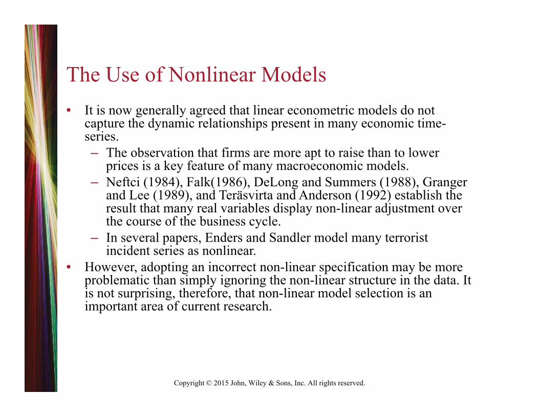
The Use of Nonlinear Models• It is now generally agreed that linear econometric models do not

capture the dynamic relationships present in many economic time-series. – The observation that firms are more apt to raise than to lower

prices is a key feature of many macroeconomic models. – Neftci (1984), Falk(1986), DeLong and Summers (1988), Granger

and Lee (1989), and Teräsvirta and Anderson (1992) establish the result that many real variables display non-linear adjustment over the course of the business cycle.

– In several papers, Enders and Sandler model many terrorist incident series as nonlinear.

• However, adopting an incorrect non-linear specification may be more problematic than simply ignoring the non-linear structure in the data. It is not surprising, therefore, that non-linear model selection is an important area of current research.


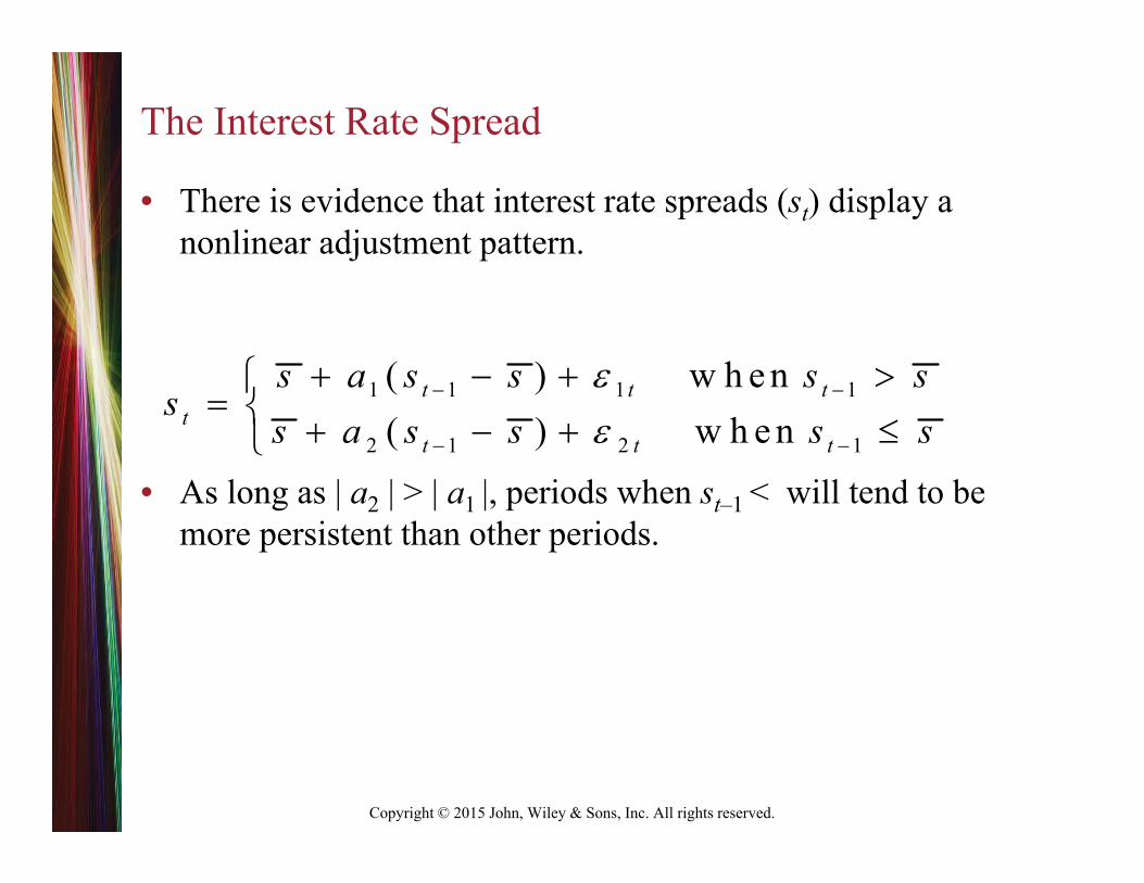
The Interest Rate Spread

• There is evidence that interest rate spreads (st) display a nonlinear adjustment pattern.

• As long as | a2 | > | a1 |, periods when st–1 < will tend to be more persistent than other periods.

1 1 1 1

2 1 2 1

( ) w h e n( ) w h e n

t t tt

t t t

s a s s s ss

s a s s s s


yt‐1

yt

yt = 1yt‐1

‐1

+1

} 11 {

2

Symmetric vs Asymmetric Adjustment


{ A A'

Figure 7.1: Two Nonlinear Adjustment Paths

Panel a Panel b

+1

-1 0

A

B

0.50

yt

a1

a1/2

-a1

a1

yt-1

yt

yt = a1yt-1

-1

+1 a1 +2

} } 2a1

B

yt = a2yt-1


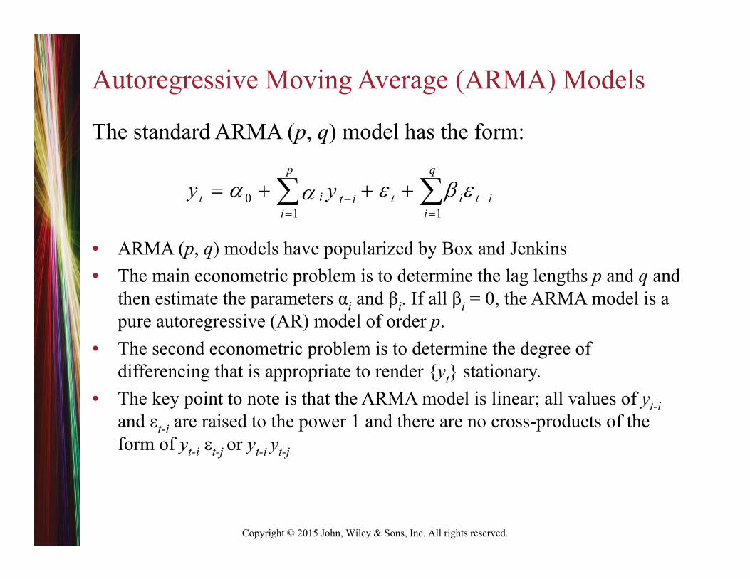
Autoregressive Moving Average (ARMA) Models

The standard ARMA (p, q) model has the form:

• ARMA (p, q) models have popularized by Box and Jenkins• The main econometric problem is to determine the lag lengths p and q and

then estimate the parameters αi and βi. If all βi = 0, the ARMA model is a pure autoregressive (AR) model of order p.

• The second econometric problem is to determine the degree of differencing that is appropriate to render {yt} stationary.

• The key point to note is that the ARMA model is linear; all values of yt-iand εt-i are raised to the power 1 and there are no cross-products of the form of yt-i εt-j or yt-i yt-j

01 1

p q

it t i t it ii i

y y


The NLAR(p) Model

• The p-th order nonlinear autoregressive model is:

• For an NLAR(2), a Taylor series expansion is

1 2( , ,..., )t t t t p ty f y y y

2 20 1 1 2 2 12 1 2 11 1 22 2

2 2 3 3112 1 2 122 1 2 111 1 222 2

t t t t t t t

t t t t t t t

y a a y a y a y y a y a y

a y y a y y a y a y


Generalized Autoregressive (GAR) ModelsThe general form of a GAR model is:

where: p, q, r, s, and u are integers that are greater or equal to 1.

• GAR models extend AR models by adding various powers of lagged values and cross-products of yt-i. Since GAR models are linear in their parameters, they can be estimated using OLS.

• You can use traditional t-tests and F-tests to pare down the number of parameters estimated. However, this can be tricky since the regressors are likely to be highly correlated. As such, the usual practice is to pare down the equation using the AIC or SBC.

tl

j-tk

i-tijkl

u

=1l

s

=1k

r

j=1

q

=1ii-ti

p

=1i0t + y y y + = y +


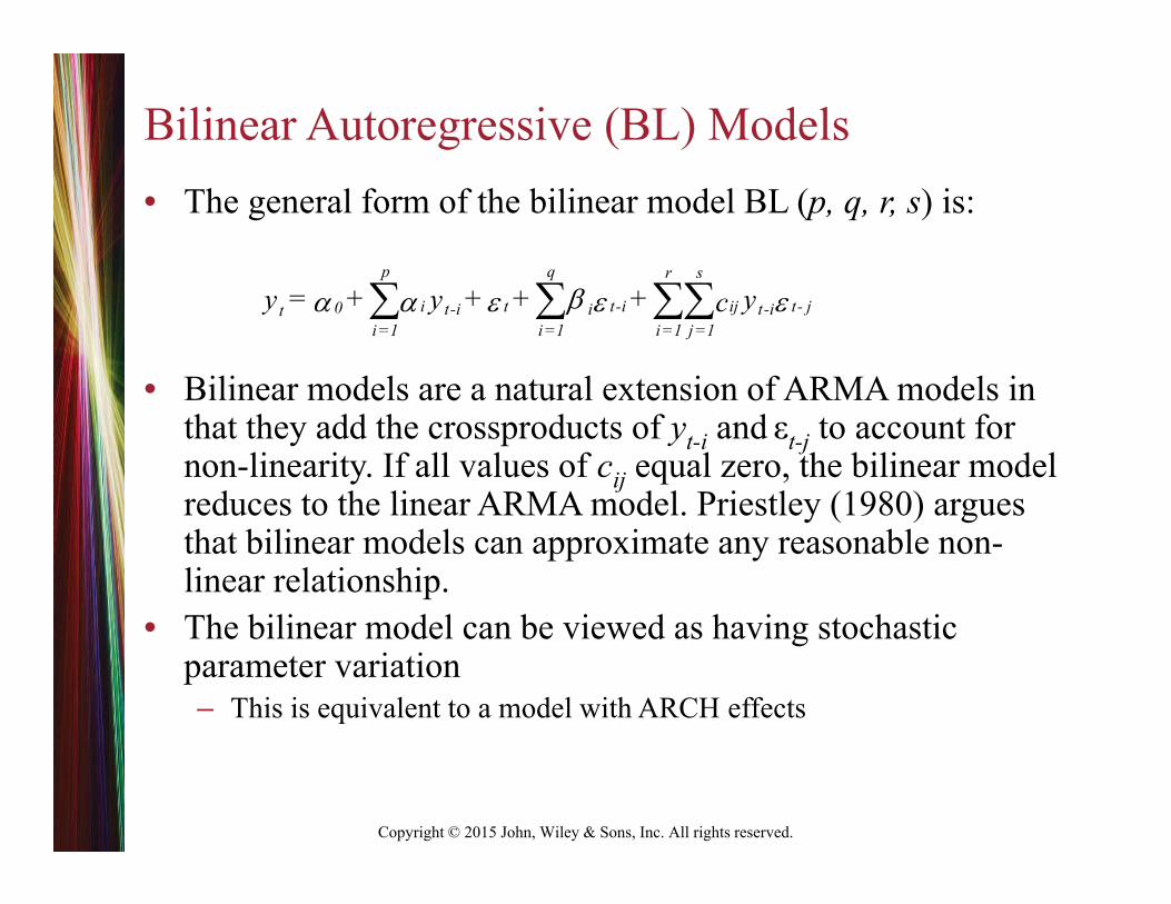
Bilinear Autoregressive (BL) Models• The general form of the bilinear model BL (p, q, r, s) is:

• Bilinear models are a natural extension of ARMA models in that they add the crossproducts of yt-i and εt-j to account for non-linearity. If all values of cij equal zero, the bilinear model reduces to the linear ARMA model. Priestley (1980) argues that bilinear models can approximate any reasonable non-linear relationship.

• The bilinear model can be viewed as having stochastic parameter variation– This is equivalent to a model with ARCH effects

p q r s

i t t-i ij t- j0 t-i i t-iti =1 i =1 i =1 j =1

= + + + +y y yc


Figure 7.2: Comparison of Linear and Nonlinear Processes

Panel a: AR

25 50 75 100 125 150 175 200-5

-4

-3

-2

-1

0

1

2

3

Panel c: Bilinear

25 50 75 100 125 150 175 200-5

-4

-3

-2

-1

0

1

2

3

Panel b: GAR

25 50 75 100 125 150 175 200-5

-4

-3

-2

-1

0

1

2

3

Panel d: TAR

25 50 75 100 125 150 175 200-5

-4

-3

-2

-1

0

1

2

3


Rothman’s unemployment estimates (1998)

AETS 3rd. edition 12

AR ut = 1.563ut–1 – 0.670ut–2 + t(22.46) (–10.06)

GAR ut = 1.500ut–1 – 0.553ut–2 – 0.745 (ut‐2 )3 + t variance ratio = 0.965(23.60) (–6.72) (–2.33)

BL ut = 1.910ut–1 – 0.690ut–2 – 0.585ut–1t–3 + t variance ratio = 0.936(24.11) (–10.55) (–2.08)

where ut = the detrended log of the unemployment rate over the 1948Q1 to1979Q4 period

The AIC was used to select the most appropriate values of p and q


Rothman II

• It is instructive to write the estimated GAR model as

ut = 1.500ut–1 – [0.553+ 0.745(ut–2)2 ] ut–2 + t

As such, large deviations are less persistent. For the bilinear model:

ut = 1.910ut–1 – 0.690ut–2 – 0.585ut–1t–3 + t

Rothman indicates that ut–1 and t–3 are positively correlated. Since the coefficient on ut–1t–3 is negative, large shocks to the unemployment rate imply a faster speed of adjustment than small shocks. As ut–1 and t–3 tend to move together, the larger ut–1t–3, the smaller is the degree of persistence.



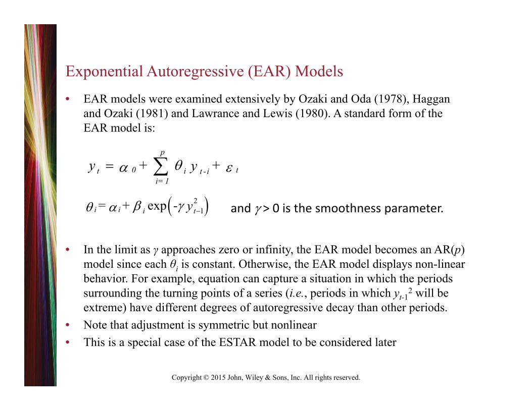
Exponential Autoregressive (EAR) Models• EAR models were examined extensively by Ozaki and Oda (1978), Haggan

and Ozaki (1981) and Lawrance and Lewis (1980). A standard form of the EAR model is:

• In the limit as γ approaches zero or infinity, the EAR model becomes an AR(p) model since each θi is constant. Otherwise, the EAR model displays non-linear behavior. For example, equation can capture a situation in which the periods surrounding the turning points of a series (i.e., periods in which yt-1

2 will be extreme) have different degrees of autoregressive decay than other periods.

• Note that adjustment is symmetric but nonlinear• This is a special case of the ESTAR model to be considered later

p

0 tt i t -ii= 1

y + + y

21expi i i t = + - y and > 0 is the smoothness parameter.


The ACF Can be Misleading in a Nonlinear ModelCorrelation is only a measure of linear association. Consider:

yt = yt-1xt-1 + μt

where: yt is observable but μt and xt are both white noise.Here, all k (for k > 0) are zero.

E[yt yt-k] = 2E[(yt-1xt-1 + μt)(yt-kxt-k + μt-k)] = 2*0

Also, all cross correlations are zero. Consider:

E[yt xt-k] = E[(yt-1xt-1 + μt)xt-k]= *0 for k 1= Var(x)Eyt-1 = 0

However, the optimal non-linear one-step ahead forecast is: βytxt.• Also, data generated by an explosive process AR(1) process will have

an ACF like that from a stationary AR(1) process.


Some Tests for Nonlinearity

• McLeod–Li (1983) test: Since we are interested in nonlinear relationships in the data, a useful diagnostic tool is to examine the ACF of the squares or cubed values of a series. – Let i denote the sample correlation coefficient between

squared residuals and use the Ljung–Box statistic to determine whether the squared residuals exhibit serial correlation.

2

1

( 2) /( )n

ii

Q = T T T i

2 2 20 1 1ˆ ˆ ˆ= ...t t n t n te e e v


Regression Error Specification Test (RESET)

• STEP 1: Estimate the best-fitting linear model. Let {et} be the residuals from the model

• STEP 2: Select a value of H (usually 3 or 4) and estimate the regression equation:

2

ˆH

ht t h t

h

e z y

where zt is the vector that contains the variables included in the model estimated in Step 1.

Hence, you can reject linearity if the sample value of the F-statistic for the null hypothesis 2 = = H = 0 exceeds the critical value from a standard F-table.

The idea is that this regression should have little explanatory power if the model is truly linear.


Specific Testing for Nonlinearity

• Lagrange Multiplier Tests– You need not estimate the nonlinear model– They have a specific alternative hypothesis– Unfortunately, they detect many types of nonlinearity

• Methodology—H0: The model has a particular linear form against a specific alternative.– Step 1. Estimate the linear portion of the model to get the residuals et

(i.e., estimate the model under H0)– Step 2. Regress et on f( )/ evaluated at the constrained values of . – Step 3. From the regression in Step 2, it can be shown that: TR2 ~ χ2

with degrees of freedom equal to the number of restrictions. Thus, if the calculated value of TR2 exceeds that in a χ2 table, reject H0.

• With a small sample, it is standard to use an F-test.


Example 1

• yt = a0 + a1yt-1 + a2yt-1yt-2 + t– H0: a2 = 0

• In this case you can estimate the nonlinear model and perform a t-test on a2. However to illustrate the procedure:

• Step 1: Estimate the model under H0 to get the estimated residuals; i.e., estimate– yt = a0 + a1yt-1 + et

• Step 2: The partial derivatives of yt w.r.t. parameters are 1, yt-1 and yt-1yt-2. Hence, regress the residuals on a constant, yt-1 and yt-1yt-2

• Step 3: Find TR2. This is χ2 with 1 degree of freedom


Example 2: Bilinear Modelyt = a0 + a1yt-1 + a2yt-2+ yt-2εt-1 + εt

Ho: γ = 0

• Regress yt on a constant yt-1 and yt-2 to obtain et

• Regress et on a constant, yt-1 , yt-2, and yt-2εt-1


THRESHOLD AUTOREGRESSIVE MODELS

• As in the equation for the spread, if we include a disturbance term, the basic TAR model is

• If we assume that the variances of the two error terms are equal [i.e., var(1t) = var(2t)]

• where It = 1 if yt–1 > 0 and It = 0 if yt–1 0.• The indicator can also be set using yt

1 1 1 1

2 1 2 1

if 0if 0

t t tt

t t t

a y yy

a y y

1 1 2 1(1 )t t t t t ty a I y a I y


The Standard TAR Model

• Consider

• where It = 1 if yt–1 > and It = 0 if yt–1 .

10 1 20 2

1 1(1 )

p r

tt t i t i t i t ii i

y I + y + I + y


The M-TAR Model

• The momentum threshold autoregressive (M-TAR) model used by Enders and Granger (1998) allows the regime to change according to the first-difference of {yt-1}. Hence, equation is replaced with:

• It is argued that the M-TAR model is useful for capturing situations in which the degree of autoregressive decay depends on the direction of change in {yt}.

• Enders and Granger (1998) and Enders and Siklos (2001) show that interest rate adjustments to the term-structure relationship display M-TAR behavior. It is important to note that for the TAR and M-TAR models, if all 1i = 2i the TAR and M-TAR models are equivalent to an AR(p) model.

• See TAR_figure.prg

1

1

10 .

tt

t

if yI

if y


Extensions

• Selecting the Delay Parameter• Multiple Regimes

– band-TAR

st = +a1(st–1 ) + t when st–1 > + cst = st–1 + t when – c < st–1 + cst = +a2(st–1 – ) + t when st–1 – c


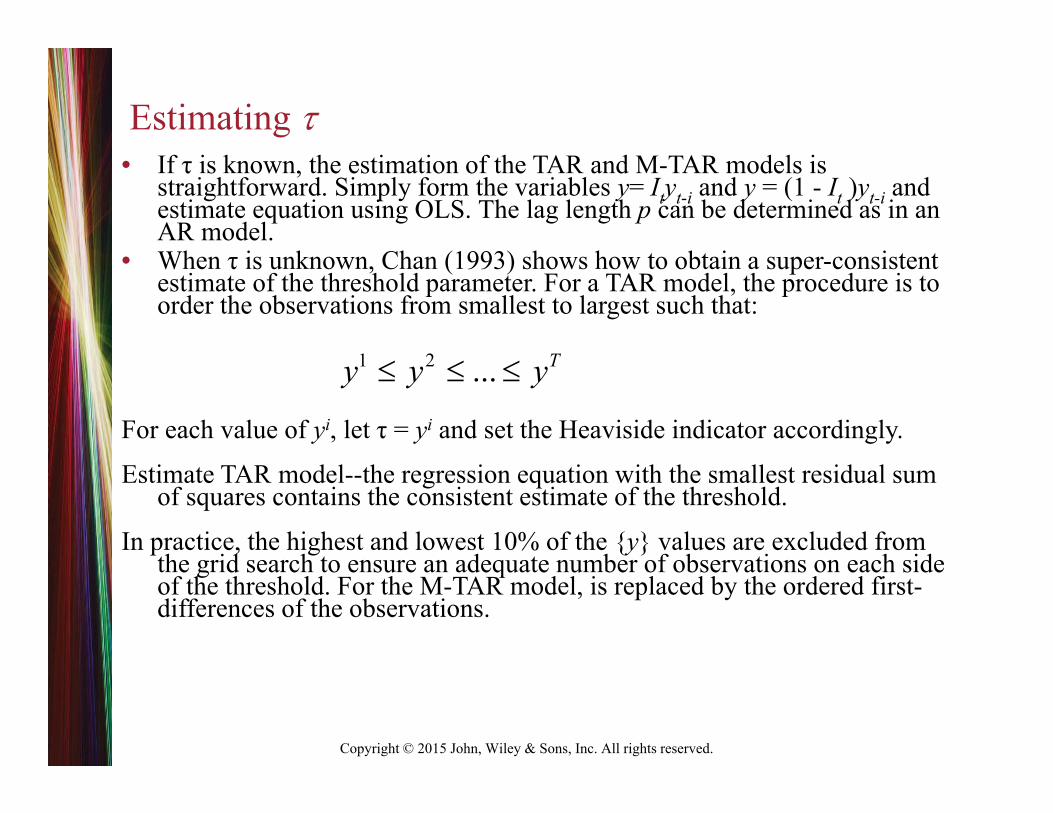
Estimating • If τ is known, the estimation of the TAR and M-TAR models is

straightforward. Simply form the variables y= Ityt-i and y = (1 - It )yt-i and estimate equation using OLS. The lag length p can be determined as in an AR model.

• When τ is unknown, Chan (1993) shows how to obtain a super-consistent estimate of the threshold parameter. For a TAR model, the procedure is to order the observations from smallest to largest such that:

For each value of yi, let τ = yi and set the Heaviside indicator accordingly.

Estimate TAR model--the regression equation with the smallest residual sum of squares contains the consistent estimate of the threshold.

In practice, the highest and lowest 10% of the {y} values are excluded from the grid search to ensure an adequate number of observations on each side of the threshold. For the M-TAR model, is replaced by the ordered first-differences of the observations.

1 2 ... Ty y y


-5

-4

-3

-2

-1

0

1

2

3

4

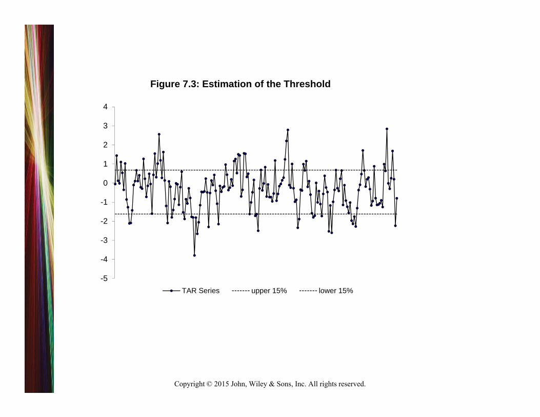
Figure 7.3: Estimation of the Threshold

TAR Series upper 15% lower 15%


-5

-4

-3

-2

-1

0

1

2

3

4

0 20 40 60 80 100 120 140 160 180 200

Thre

shol

dsFigure 7.4: Ordered Threshold Values

Ordered lower 15% upper 15%


Figure 7.7: SSR and the Potential ThresholdsPotential Thresholds

SSR

-0.20 -0.10 -0.00 0.10 0.20

14.2

14.3

14.4

14.5

14.6

14.7


Figure 7.6 The U.S. Unemployment Rate

Perc

ent

1960 1965 1970 1975 1980 1985 1990 1995 2000 2005 20103

4

5

6

7

8

9

10

11


Unidentified Nuisance Parameters

• Example 1:– Estimate by NLLS. Under the null 2 = 0, the model

becomes

• Example 2. yt = 0 + 1yt−1 + 2Dt + t

– Dt = 1 if t ≥ t* and Dt = 0 otherwise. If the break date t* is unknown, t* is an unidentified nuisance parameter.

• Example 3: yt = 0+1/[1 + exp(−γyt−1)] + t.– if is unknown, a test for linearity implies γ = 0 so that yt = 0 + 1/2 + t (since exp(0) = 1).

– Similarly if 1 = 0, the model becomes yt = 0 + t so that is not identified in that its value is irrelevant.


20 1t t ty x

0 1t ty


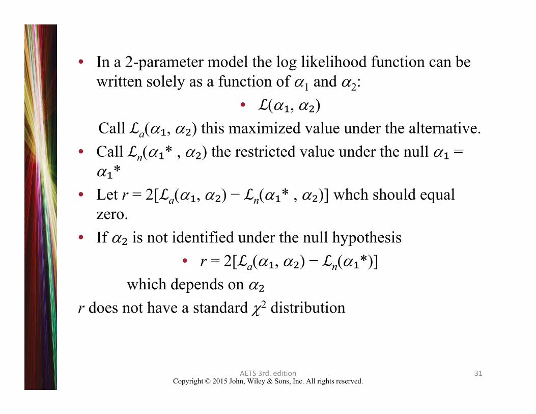
• In a 2-parameter model the log likelihood function can be written solely as a function of 1 and 2:

• (₁, ₂)Call a(₁, ₂) this maximized value under the alternative.

• Call n(₁* , ₂) the restricted value under the null ₁ = ₁*

• Let r = 2[ a(₁, ₂) − n(₁* , ₂)] whch should equal zero.

• If ₂ is not identified under the null hypothesis • r = 2[ a(₁, ₂) − n(₁*)]

which depends on ₂r does not have a standard 2 distribution



Inference

• Inference on the coefficients in a threshold model is not straightforward since it was necessary to search for . Under the null of linearity is not identified.

• The t-statistics yield only an approximation of the actual significance levels of the coefficients. The problem is that the coefficients on the various ut-i are multiplied by It or (1It) and that these values are dependent on the estimated value of .

• The percentile and bootstrap t methods can be used


Hansen’s (1997) supremum test.

• You cannot perform a traditional F-test. • To use Hansen’s (1997) bootstrapping method, you need to draw T

normally distributed random numbers with a mean of zero and a variance of unity; let et denote this set of random numbers. You treat et as the dependent variable. Regress et on the actual values of yt–i to obtain an estimate of SSRr called SSRr

*. • For each potential value of regress et on Ityt–1 and (1 – It)yt–1 [i.e.,

estimate a regression in the form et = Ityt–1 + (1 – It)yt–1] and use the regression providing the best fit. Call the sum of squared residuals from this regression SSRu

*. Use these two sums of squares to form

• Repeat this process several thousand times to obtain the distribution of F*.


* **

*

( ) /( /( 2 ))

r u

u

SSR SSR nFSSR T n


Threshold Regression Models

• yt = a0 + (a1 + b1It)xt + t

where It = 1 if yt–d > and It = 0 otherwise.

• Pretesting for a TAR Model

However, the F-statistic needs to be bootstrapped. (see Hansen above)

( ) /( /( 2 ))

r u

u

SSR SSR nFSSR T n


TAR Models and Endogenous Breaks

• The threshold model is equivalent to a model with a structural break. The only difference is that in a model with structural breaks, time is the threshold variable.

• Carrasco (2002) shows that the usual tests for structural breaks (i.e., those using dummy variables) have little power if the data are actually generated by a threshold process– However, a test for a threshold process using yt-d as the

threshold variable has power to detect both threshold behavior and structural change. Even if there is a single structural break at time period t, using yt-d as the threshold variable will mimic this type of behavior.

– As such, she recommends using the threshold model as a general test for parameter instability.


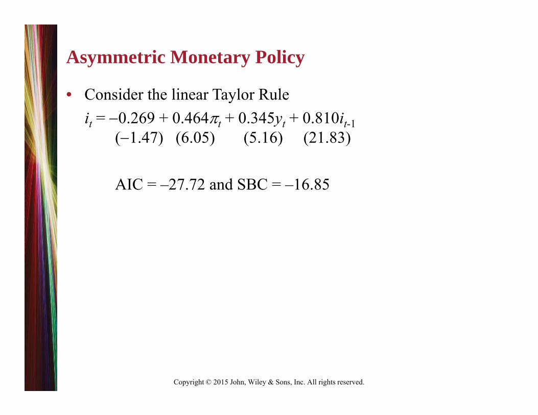
Asymmetric Monetary Policy

• Consider the linear Taylor Ruleit = 0.269 + 0.464t + 0.345yt + 0.810it-1

(1.47) (6.05) (5.16) (21.83)

AIC = –27.72 and SBC = –16.85


The TAR Taylor Rule• Since we do not know the delay factor, we can estimate four threshold

regressions with πt-1, πt-2, yt-1 and yt-2 as the threshold variables

it = 1.421 + 1.051t + 0.469yt + 0.374it-1 when πt-2 3.527(3.15) (10.55) (6.22) (5.74)

and

it = –0.456 + 0.232t + 0.302yt + 0.959it-1 when πt-2 < 3.527(–1.40) (1.88) (3.77) (24.55)

τ SSR AIC BIC πt-1 3.527 50.80 –70.55 –46.08 πt-2 3.668 50.42 –71.39 –46.93 yt-1 –1.183 63.97 –44.73 –20.26 yt-2 –1.565 53.51 –64.94 –40.47


Capital Stock Adjustment with Multiple Thresholds

• For our purposes, the key variables in the Boetel, Hoffman and Liu (2007) model are

Kt – Kt-1 = 4569 + 6360 I1t + 6352 I2t + 452pHt-1 – 2684pFt-1 + … (3.30) (5.59) (5.20) (1.84) (–3.66)

• where: Kt is the size of the breeding stock, pHt-1 is a measure of the output price of hogs, and pFt-1 is a measure of the price of feed. The indicators functions are such that I1t = 1 if pHt-1 > τhigh = 1.1185 and I2t = 1 if pHt-1 < τlow = 1.1105. The use of lagged values for the dependent variables is designed to reflect a one period delay between the time of the investment decision and its realization.

– allowing all variables to have asymmetric effects on Kt – Kt-1 would entail estimating a large number of parameters with a consequent loss of degrees of freedom.


Capital Stock Adjustment with Multiple Thresholds II

• … the three regimes are distinguished by pHt-1 relative to two threshold values.

• when pHt-1 is between τhigh and τlow, I1t and I2t = 0 so that the intercept is 4569.

• when pHt-1 > τhigh, I1t = 1 the intercept is 10929 and when pHt-1< τlow, I2t = 1 the intercept is 8.

• Thus, there is a high-, sluggish- and disinvestment regime whose presence is dependent on the value of pHt-1.

• It would be a mistake to conclude that the slope coefficient 452 measures the full effect of a price change on net investment. When the value of pHt-1 crosses one of the thresholds, the change in investment is enhanced since the intercept changes along with the price. Also note that price changes within the interval τhigh to τlow, will little effect on investment.


Smooth Transition Models

• In some instances, it may not be reasonable to assume that there are 2 pure regimes:– Multi-regime TAR model– It is possible to assume that the transition is smooth

• Smooth transition autoregressive (STAR) models allow the autoregressive parameters to change slowly:– yt = α0 + α1yt-1 + β1yt-1f [ yt-1 - μ ] + εt

where: f [ ] is a continuous function.Typically: f(0) = 1 and f(±) = 0 (as in a density function).when yt-1 = μ, autoregressive decay is α1 + β1 and when |yt-1 - μ| is

large, decay is α1.


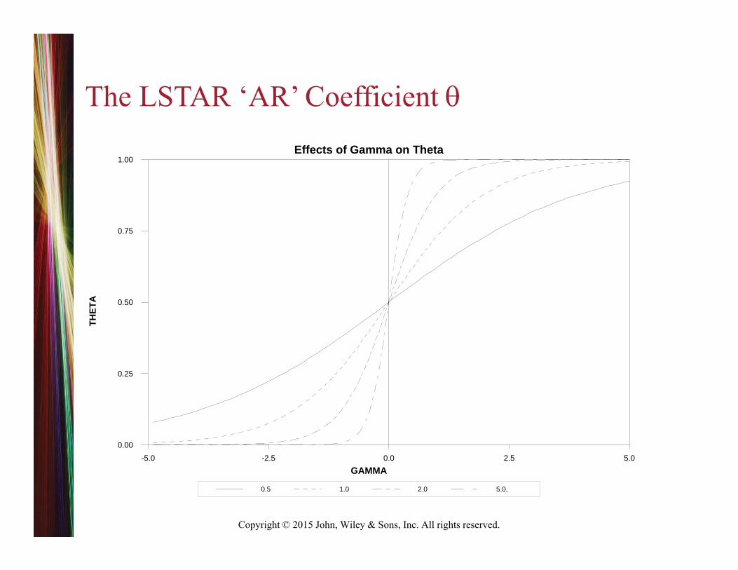
The Logistic Smooth Transition Autoregressive (LSTAR) Model• The LSTAR model generalizes the standard autoregressive model to allow

for a varying degree of autoregressive decay.

• In the limit as 0 or , the LSTAR model becomes an AR(p) model since each value of θ is constant.

• For intermediate values of , the degree of autoregressive decay depends on the value of yt-1. As yt-1 - , θ 0 so that the behavior of yt is given by 0 + 1yt-1 + … + pyt-p + t. As yt-1 + , θ 1 so that the behavior of yt is given by (0 + 0) + (1 + 1) yt-1 + … + (p + p) yt-p + t.

0 01 1

( )p p

t i t i i t i ti i

y y y

11[1 exp ]t= + - y c and γ > 0 is a scale parameter


0.5 1.0 2.0 5.0,

Effects of Gamma on Theta

GAMMA

THET

A

-5.0 -2.5 0.0 2.5 5.00.00

0.25

0.50

0.75

1.00

The LSTAR ‘AR’ Coefficient


Pretesting for an LSTAR Model


1 1[1 exp( ( ))] [1 exp( )]t d t dy c h

For the LSTAR model:

Use a third-order Taylor series approximation of with respect to ht–d evaluated ht–d = 0. Of course, this is identical to evaluating the expansion at = 0.

/ ht–d exp(–ht–d)/[1 + exp(–ht–d)]2 1/4

2nd deriv. exp(–ht–d)[1 – exp(–ht–d)]/[1 + exp(–ht–d)]3 0

3rd deriv exp(–ht–d)[1+exp(–2ht–d) – 4exp(–ht–d)]/[1 + exp(–ht–d)]4 –1/8

3tdh

yt = 0 + 1yt–1 + … + pyt–p + (0 + 1yt–1 + … + pyt–p )(1ht–d + 3 (ht-d)3) + t

Because ht–d depends only on the value of yt–d, we can write the model in the more compact form:can test for the presence of LSTAR behavior by estimating an auxiliary regression:

et = a0 + a1yt–1 + … + apyt–p + a11yt–1yt–d + … + a1pyt–pyt–d + a21yt–1 + … + a2pyt–1+ a31yt–1 + … + a3pyt–p + t. (7.21)


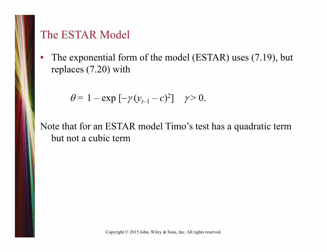
The ESTAR Model

• The exponential form of the model (ESTAR) uses (7.19), but replaces (7.20) with

= 1 – exp [ (yt–1 – c)2] > 0.

Note that for an ESTAR model Timo’s test has a quadratic term but not a cubic term

Copyright © 2015 John, Wiley & Sons, Inc. All rights reserved.AETS 3rd. edition 45


Pretesting for an ESTAR Model


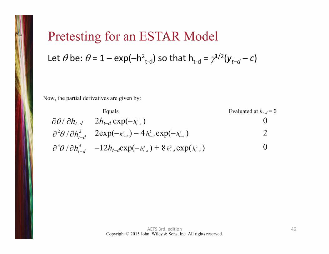
Let be: = 1 – exp(–h2t‐d) so that ht‐d = 1/2(yt–d – c)

2t dh )

Now, the partial derivatives are given by:

Equals Evaluated at ht–d = 0

/ ht–d 2ht–d exp(– 2t dh ) 0

2 2/ t dh 2exp(– 2t dh ) – 4 2

t dh exp(– 2t dh ) 2

3 3/ t dh –12htdexp(– 2t dh ) + 8 3

t dh exp( 2t dh ) 0


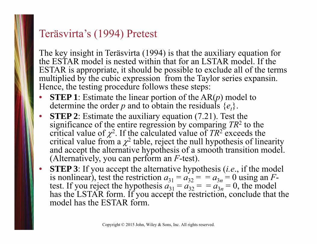
Teräsvirta’s (1994) Pretest

The key insight in Teräsvirta (1994) is that the auxiliary equation for the ESTAR model is nested within that for an LSTAR model. If the ESTAR is appropriate, it should be possible to exclude all of the terms multiplied by the cubic expression from the Taylor series expansin. Hence, the testing procedure follows these steps:• STEP 1: Estimate the linear portion of the AR(p) model to

determine the order p and to obtain the residuals {et}. • STEP 2: Estimate the auxiliary equation (7.21). Test the

significance of the entire regression by comparing TR2 to the critical value of 2. If the calculated value of TR2 exceeds the critical value from a 2 table, reject the null hypothesis of linearity and accept the alternative hypothesis of a smooth transition model. (Alternatively, you can perform an F-test).

• STEP 3: If you accept the alternative hypothesis (i.e., if the model is nonlinear), test the restriction a31 = a32 = = a3n = 0 using an F-test. If you reject the hypothesis a31 = a32 = = a3n = 0, the model has the LSTAR form. If you accept the restriction, conclude that the model has the ESTAR form.


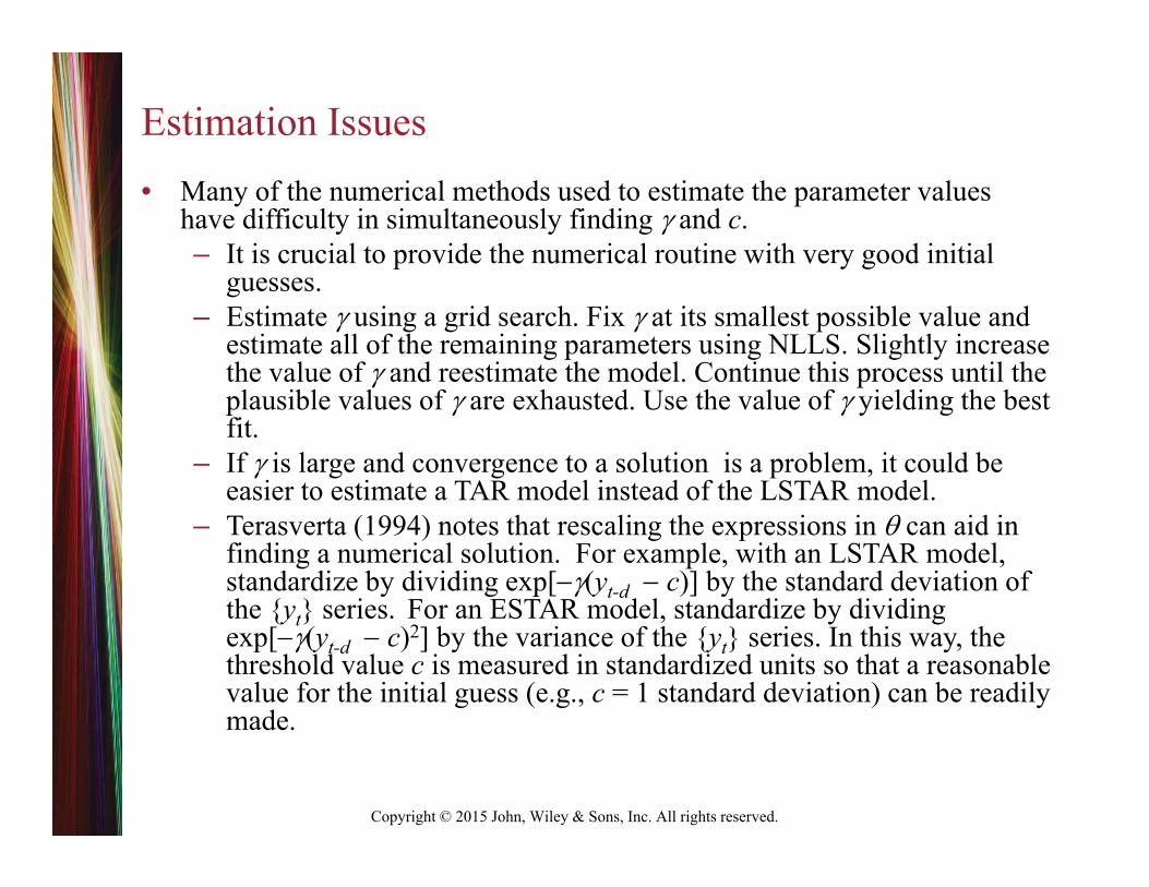
Estimation Issues• Many of the numerical methods used to estimate the parameter values

have difficulty in simultaneously finding and c. – It is crucial to provide the numerical routine with very good initial

guesses. – Estimate using a grid search. Fix at its smallest possible value and

estimate all of the remaining parameters using NLLS. Slightly increase the value of and reestimate the model. Continue this process until the plausible values of are exhausted. Use the value of yielding the best fit.

– If is large and convergence to a solution is a problem, it could be easier to estimate a TAR model instead of the LSTAR model.

– Terasverta (1994) notes that rescaling the expressions in can aid in finding a numerical solution. For example, with an LSTAR model, standardize by dividing exp[(yt-d c)] by the standard deviation of the {yt} series. For an ESTAR model, standardize by dividing exp[(yt-d c)2] by the variance of the {yt} series. In this way, the threshold value c is measured in standardized units so that a reasonable value for the initial guess (e.g., c = 1 standard deviation) can be readily made.


Michael, Nobay, and Peel (1997)

• yt = 0.40yt–1 + [1 – exp(–532.4(yt–1 – 0.038)2] (–yt–1

+ 0.59yt–2 + 0.57yt–4 – 0.017)

The point estimates imply that when the real rate is near 0.038, there is no tendency for mean reversion since a1 = 0. However, when (yt–1 – 0.038)2 is very large, the speed of adjustment coefficient is quite rapid. Hence, the adjustment of the real exchange rate is consistent with the presence of transaction costs.


11. UNIT ROOTS AND NONLINEARITY

• yt = It1(yt–1 – ) + (1 – It)2(yt–1 – ) + t (7.30)

1

1

10

tt

t

if yI

if y

STEP 1: If you know the value of (for example = 0), estimate (7.30). Otherwise, use Chan’s method: select the value of from the regression containing the smallest value for the sum of squared residuals. STEP 2: If you are unsure as to the nature of the adjustment process, repeat Step 1 using the M‐TAR model. STEP 3: Calculate the F‐statistic for the null hypothesis 1 = 2 = 0. For the TAR model, compare this sample statistic with the appropriate critical value in Table G. STEP 4: If the alternative hypothesis is accepted (i.e., if there is an attractor), it is possible to test for symmetric versus asymmetric adjustment since the asymptotic joint distribution of 1 and 2 converges to a multivariate normal.


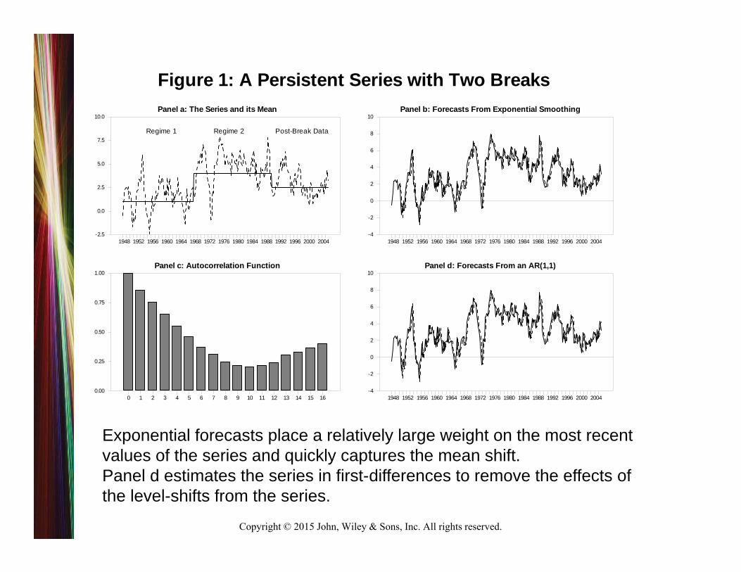
Old School versus New School‘Old School’ forecasting techniques, such as exponential

smoothing and the Box-Jenkins methodology, do not attempt to explicitly model or to estimate the breaks in the series. – Exponential smoothing: place relatively large weights on the

most recent values of the series. – The Box-Jenkins: first-difference or second difference the series

in order to control for the lack of mean reversion. • Differencing can be chosen by the autocorrelation function

or by some type of Dickey-Fuller test. ‘New School’ forecasters attempt to estimate the number and

magnitudes of the breaks. Given that the breaks are well-estimated, it is possible to control for the regime shifts when forecasting.


Figure 1: A Persistent Series with Two BreaksPanel a: The Series and its Mean

1948 1952 1956 1960 1964 1968 1972 1976 1980 1984 1988 1992 1996 2000 2004-2.5

0.0

2.5

5.0

7.5

10.0

Regime 1 Regime 2 Post-Break Data

Panel c: Autocorrelation Function

0 1 2 3 4 5 6 7 8 9 10 11 12 13 14 15 160.00

0.25

0.50

0.75

1.00

Panel b: Forecasts From Exponential Smoothing

1948 1952 1956 1960 1964 1968 1972 1976 1980 1984 1988 1992 1996 2000 2004-4

-2

0

2

4

6

8

10

Panel d: Forecasts From an AR(1,1)

1948 1952 1956 1960 1964 1968 1972 1976 1980 1984 1988 1992 1996 2000 2004-4

-2

0

2

4

6

8

10

Exponential forecasts place a relatively large weight on the most recent values of the series and quickly captures the mean shift.Panel d estimates the series in first-differences to remove the effects of the level-shifts from the series.


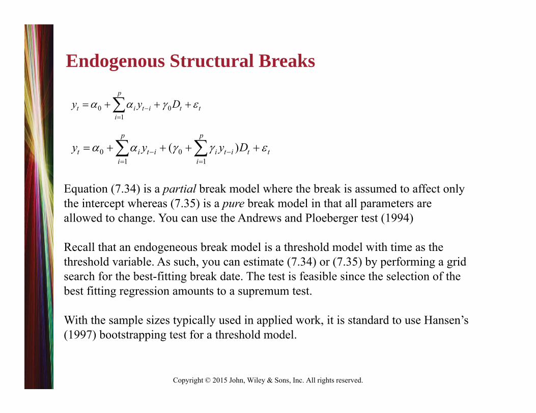
Endogenous Structural Breaks

0 01

p

t i t i t ti

y y D

0 01 1

( )p p

t i t i i t i t ti i

y y y D

Equation (7.34) is a partial break model where the break is assumed to affect only the intercept whereas (7.35) is a pure break model in that all parameters are allowed to change. You can use the Andrews and Ploeberger test (1994)

Recall that an endogeneous break model is a threshold model with time as the threshold variable. As such, you can estimate (7.34) or (7.35) by performing a grid search for the best-fitting break date. The test is feasible since the selection of the best fitting regression amounts to a supremum test.

With the sample sizes typically used in applied work, it is standard to use Hansen’s (1997) bootstrapping test for a threshold model.


Bai and Peron: Multiple Breaks

0 1 1 2 21

( .... )p

t i t i t t m mt ti

y y D D D

0 01 1 1

( )p pm

t i t i jt j ij t i ti j i

y y D y

Bai and Perron develop a supremum test for the null hypothesis of no structural change (m = 0) versus the alternative hypothesis of m = kbreaks.

The second method of selecting the number of breaks is to use a sequential test.


Supremum

Estimate models for every possible combination of breaks (given the trimming and minimum break size) and select the best fitting combination of break dates.

The appropriate F-statistic, called the F(k; q) statistic, is nonstandard; the critical values depend on the number of breaks, k, and the number of breaking parameters, q.

If the null hypothesis of no breaks is rejected, they select the actual number of breaks using the SBC. For q = 1, 2, and 3, the 95% critical for 1, 2, and 5 breaks are:

q k = 1 k = 2 k = 5 UDmax1 9.63 8.78 6.69 10.172 12.89 11.60 9.12 13.273 15.37 13.84 11.15 16.82


Sequential Method

• Begin with the null hypothesis of no-breaks versus the alternative of a single break. If the null hypothesis of no breaks is rejected, proceed to test the null of a single break versus two breaks, and so forth.

• The method is sequential in that the test for break l + 1 takes the first l breaks as given. At each stage, the so-called sup F(l+1| l)statistic is calculated as the maximum F-statistic for the null hypothesis of no additional against the alternative of one additional break. For q = 1, 2, and 3, the 95% critical for = 0, 1, 2, and 5 are:

q = 0 = 1 = 2 = 4 1 9.63 11.14 12.16 13.452 12.89 14.50 15.42 16.613 15.37 17.15 17.97 19.23


Fourier Breaks (see www.time-series.net)

A simple modification of the standard autoregressive model is to allow the intercept to be a time-dependent function

Although (1) is linear in {yt}, the specification is reasonably general in that d(t) can be a deterministic polynomial expression in time, a p-th order difference equation, a threshold function, or a switching function.


UDmax

it also seems reasonable to test the null of no breaks against the alternative of some breaks. If the largest of the F(k; q) statistics for k = 1, 2, 3 … exceeds the UDmax statistic reported above, you can conclude that there are some breaks and then go on to select the number using the SBC.


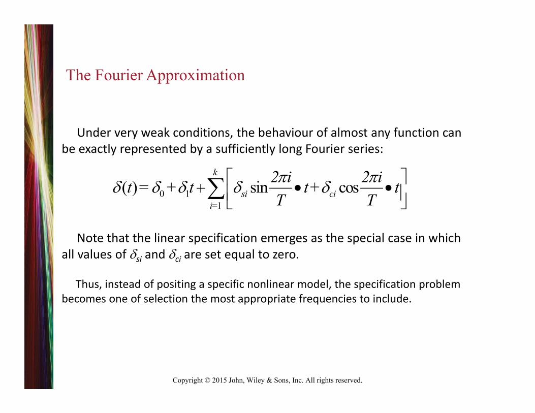
The Fourier Approximation

Under very weak conditions, the behaviour of almost any function can be exactly represented by a sufficiently long Fourier series:

Note that the linear specification emerges as the special case in which all values of si and ci are set equal to zero.

Thus, instead of positing a specific nonlinear model, the specification problem becomes one of selection the most appropriate frequencies to include.

0 11

( ) sin cosk

si cii=

2 i 2 it = + t t+ t T T



Logistic Breaks

yt = 0 + 1yt–1 + + pyt–p + [0 + 1yt–1 + + pyt–p] + t

= [1 + exp((t t*))]1


Figure 7.14 A Simulated LSTAR Break

Panel a: Bai-Perron Breaks

Bai-Perron Series

25 50 75 100 125 150 175 200 225 250-2

0

2

4

6

8

10

12Panel b: Logistic Break

Logistic Series

25 50 75 100 125 150 175 200 225 250-2

0

2

4

6

8

10

12

Date post:	10-Feb-2018
Category:	Documents
Upload:	trinhnhu
View:	218 times
Download:	2 times

ERIES RD ED ALTER ENDERS - Time...

Documents