ERPsim for SAP HANA - Reference Guide -...

ERPsim for SAP HANA

Reference Guide Authors Jean-François Michon Jacques Robert Derick Lyle Pierre-Majorique Léger Gilbert Babin

Revision 4.0 Creation Date March 8, 2015 Last Revision Date August 15, 2016 Last Update Date August 15, 2016 Language English ISBN Pending

Michon et al. (2015-2016) ERPsim Lab, HEC Montréal. 2 of 51

TABLE OF CONTENTS

An introduction to ERPsim for SAP HANA ...................................................................................................................................................................... 3

How to use this guide ................................................................................................................................................................................................ 4

Get started: Using SAP Lumira with ERPsim .................................................................................................................................................................. 5

Software and connection details ............................................................................................................................................................................... 5

Connecting to a view .................................................................................................................................................................................................. 5

The interface .............................................................................................................................................................................................................. 9

PART ONE: Using SAP HANA Views for ERPsim ........................................................................................................................................................... 11

Which view should I use? ......................................................................................................................................................................................... 13

ERPSIM_FINANCIALS_CUMULATIVE_BALANCE ....................................................................................................................................................... 15

ERPSIM_FINANCIALS_POSTINGS ............................................................................................................................................................................. 18

ERPSIM_GOODS_MOVEMENTS ............................................................................................................................................................................... 24

ERPSIM_INVENTORY ................................................................................................................................................................................................ 30

ERPSIM_MARKET ..................................................................................................................................................................................................... 34

ERPSIM_SALES ......................................................................................................................................................................................................... 38

ERPSIM_SUPPLIER_PRICES ....................................................................................................................................................................................... 44

MUESLI_PRODUCTION ............................................................................................................................................................................................. 47

Copyright Notice .......................................................................................................................................................................................................... 50

Document Revision Control ......................................................................................................................................................................................... 51


AN INTRODUCTION TO ERPSIM FOR SAP HANA

2015 marks the release of ERPsim for SAP HANA. Powered by ERPsim, an original and fun way to teach and learn ERP concepts, this version also introduce real time analytics using an in‐memory database, SAP HANA. While the simulator is also available with SAP ECC 6.07 and ERPsim BI, a technology allowing real‐time analytics using SQL Server as the data warehouse, HANA allows to tap directly in the ERP’s hearth and get meaningful knowledge about your business from its transactional data.

With this new technology becoming available, having ERPsim to be compatible with it was an evidence. Not only the game is an engaging experience for participants to learn business processes and the transactions supporting them, but having access to data that is meaningful to you will entice you to learn more on how to get the best out of it. The best part of it is that SAP Lumira, SAP’s data discovery and visualization tool, allows to do all of this in a matter of minutes, if not seconds.

We sincerely hope that you’ll enjoy this version of ERPsim!

We’d like to thanks those who contributed to and have been involved in the ERPsim for SAP HANA project:

Prof. Pierre‐Majorique Léger (Ph.D.), Prof. Jacques Robert (Ph.D.), Prof. Gilbert Babin (Ph.D.), Prof. Bret Wagner (Ph.D.), Prof. Robert Pellerin (Ph.D.) Co‐inventors of ERPsim;

Jean‐François Michon (M.Sc.), Derick Lyle (MBA), Félix Gaudet‐Lafontaine (BBA) development, management and technical team, ERPsim Lab;

Prof. Ross Hightower (Ph.D.), Jerad Lumina (MBA) development, hosting partners, UCC Milwaukee;

Hikmath‐Yemissi Eyitayo (BBA), Anne‐Laure Juvin (BBA), Pauline Laurainne (BBA), Cindy Nguyen (BBA), Arnaud Paquet (BBA), Samuel Plasse (BBA) testers and analysts, ERPsim Lab;

And also all faculty members, UCC partners and SAP University Alliances team members, who provided feedback, comments and suggestions, participated in our betas, and who believe in and support ERPsim for now more than 11 years!


HOW TO USE THIS GUIDE

This guide was built with the premise that it should be easy to consult, and allow you to get a quick reference on each view’s structure. For each view, we’ll provide you with a general description, its properties, a description of the measure, dimensions and input parameters, as well as a few examples how what you can mix‐and‐match to create useful visualizations with SAP Lumira.

The purpose of this guide is not to teach how to use Lumira, but to give you the means to use it with ERPsim. We’ve ensured the maximum compatibility with the tools provided in Lumira while developing the views: feel free to explore and discover the outcome!

Please remember that SAP Lumira is a software that is constantly evolving, with updates being released every month or so. The examples and instructions provided in this guide were created using versions 1.28.2 and 1.29.3 of SAP Lumira. If you are using a different version, please consider that elements covered in this document may be different or not valid anymore. You can review the SAP Lumira user guide and release notes at http://help.sap.com/lumira.


GET STARTED: USING SAP LUMIRA WITH ERPSIM

SOFTWARE AND CONNECTION DETAILS

Required:

SAP Lumira (latest version), which can be downloaded from http://go.sap.com/product/analytics/lumira.html. Access to the HANA system, which requires the following information:

o Connection details to be provided by your instructor. You need the Server and the Instance/port number, as well as the user account (User) and Password.

CONNECTING TO A VIEW

To establish a connection to the HANA database and start using a view:

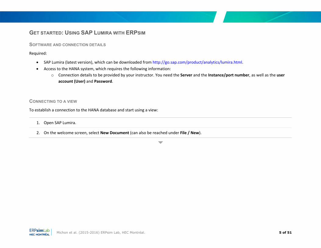
1. Open SAP Lumira.

2. On the welcome screen, select New Document (can also be reached under File / New).


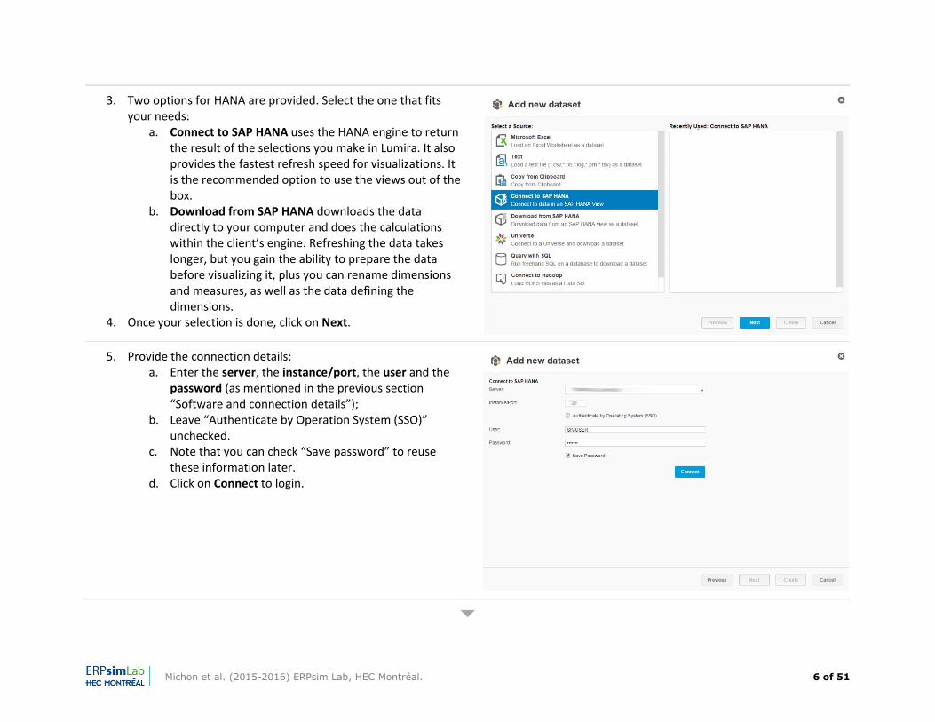
3. Two options for HANA are provided. Select the one that fits your needs:

a. Connect to SAP HANA uses the HANA engine to return the result of the selections you make in Lumira. It also provides the fastest refresh speed for visualizations. It is the recommended option to use the views out of the box.

b. Download from SAP HANA downloads the data directly to your computer and does the calculations within the client’s engine. Refreshing the data takes longer, but you gain the ability to prepare the data before visualizing it, plus you can rename dimensions and measures, as well as the data defining the dimensions.

4. Once your selection is done, click on Next.

5. Provide the connection details: a. Enter the server, the instance/port, the user and the

password (as mentioned in the previous section “Software and connection details”);

b. Leave “Authenticate by Operation System (SSO)” unchecked.

c. Note that you can check “Save password” to reuse these information later.

d. Click on Connect to login.


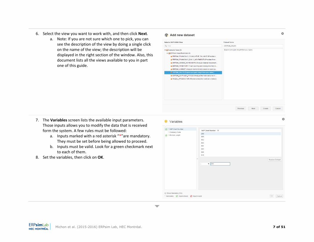
6. Select the view you want to work with, and then click Next. a. Note: If you are not sure which one to pick, you can

see the description of the view by doing a single click on the name of the view; the description will be displayed in the right section of the window. Also, this document lists all the views available to you in part one of this guide.

7. The Variables screen lists the available input parameters. Those inputs allows you to modify the data that is received form the system. A few rules must be followed:

a. Inputs marked with a red asterisk “*”are mandatory. They must be set before being allowed to proceed.

b. Inputs must be valid. Look for a green checkmark next to each of them.

8. Set the variables, then click on OK.


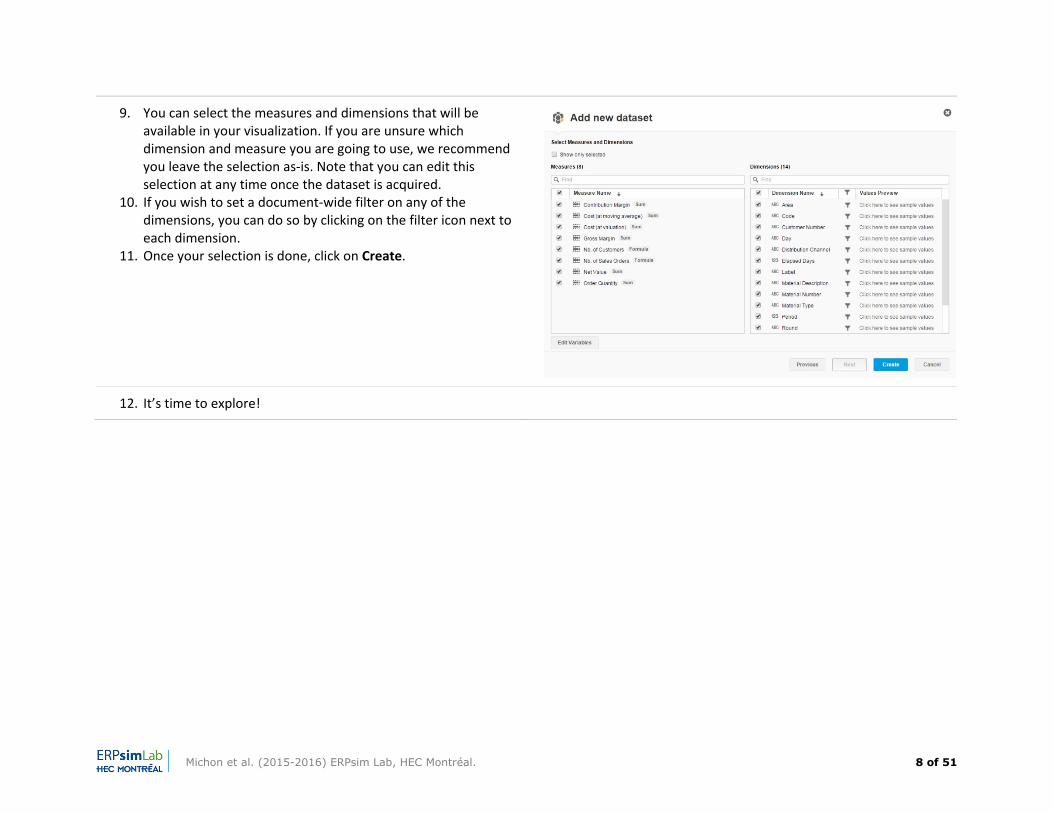
9. You can select the measures and dimensions that will be available in your visualization. If you are unsure which dimension and measure you are going to use, we recommend you leave the selection as‐is. Note that you can edit this selection at any time once the dataset is acquired.

10. If you wish to set a document‐wide filter on any of the dimensions, you can do so by clicking on the filter icon next to each dimension.

11. Once your selection is done, click on Create.

12. It’s time to explore!


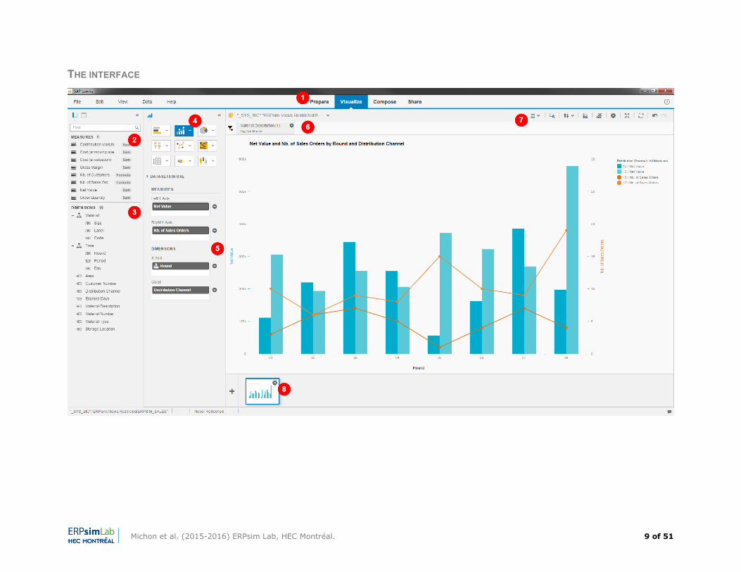
THE INTERFACE


Main elements of the interface:

1. Selection of the stage in the use of the view. a. Prepare allows to view the values that the dimensions can take. A right‐click on a value will show you all combinations to which

this data is linked. b. Visualize is the main screen of Lumira, and is also where you build your visualizations using the dimensions and measures

provided to you. c. Compose is used to create stories, which allows to review multiple visualizations on one screen. You can also apply filters, which

will be applied on all visualizations (within the storyboard). d. Share allows the exportation of stories to a file, or publish to SAP Lumira Server (this feature is not supported at this time).

2. Measures available in the view. The aggregation type is displayed next to each of them. You can also edit the properties of a measure or

create a new one by hovering the measure name and by clicking on the cog next to it. Calculated measures can be particularly useful to create ratios (ex.: Average Price = Sales Order Item Net Value / Quantity Sold) or constants (ex.: Warehouse Capacity = 250000).

3. Dimensions available in the view. Hover your mouse over a dimensions to edit its properties (by clicking on the cog).

4. Visualizations selection can be made from a variety of charts. At any time, you can switch from one chart type to another, but be warned that it may change the selection of measures and dimensions in area #5.

5. Drag‐and‐drop zone for the measures and dimensions.

6. Filters for the visualization.

7. Set options of the visualization, like display of data labels, legend, or apply conditional formatting.

8. List of visualizations that have been created and are available in the Lumira document.


PART ONE: USING SAP HANA VIEWS FOR ERPSIM

The current release of ERPsim comes with seven views, allowing you to explore your data from different angles. Whether you want to look at your sales, make sense of the market, review your performance in handling your inventory, or analyzing your financials, there is a view for that.

Each view as a scope, which mean that it will either work for certain games, or all of them. To identify the scope of the view, simply look at the first word in its name:

“ERPSIM” means that the view work with both games (Manufacturing and Logistics); “DAIRY” means that the view can only be used with the Logistics game; “MUESLI” means that the view can only be used with the Manufacturing game.

For each view, we’re providing you with the following information:

The description, the view type, and the scope of the view; The list of input parameters, which are used to filter the data that the view will return; The list of measures, which provides the calculated values. The aggregation type, which tells the type of calculation done on the values,

is indicated for each of them; The list of dimensions, which are used to regroup and explore the data returned by the measures; Recommendations and additional information regarding the view, which include recommended use of dimensions and measures

combinations, limitations to the type of data provided, and more; In some cases, we’re providing examples of custom calculated measures that can be created directly in Lumira to extend the analysis

capabilities (for example, by creating ratios or calculating average values). While not providing a complete list of measures that can be created, these examples can cover a large array of scenarios.


Currently, eight views are available. You may find their description below, and the full details at the page mentioned for each of them.

ERPSIM_FINANCIALS_CUMULATIVE_BALANCE (pages 15‐17) Provides cumulative balance for each account on a daily basis. For primarily debit accounts (assets, costs), debit increases the balance while credit decreases the balance. For primarily credit accounts (liabilities, revenues), credit increases the balance while debit decreases the balance.

ERPSIM_FINANCIALS_POSTINGS (pages 18‐23) Provides financial statements and day‐to‐day accounting transactions. Allows G/L account analysis using time series. Amounts are provided as real (debit+/credit‐ or debit‐/credit+) and absolute values (requires the use of the debit/credit indicator dimension).

ERPSIM_GOODS_MOVEMENTS (pages 23‐29) Analyze material movements across your company.

ERPSIM_INVENTORY (pages 30‐33) Track opening and closing inventory balance.

ERPSIM_MARKET (pages 34‐37) Analyze market shares based on sales quantity or net value. Compare you company's data with the competitors and / or the whole market.

ERPSIM_SALES (pages 38‐44) Explore and gain insight from your sales.

ERPSIM_SUPPLIER_PRICES (pages 45‐47) Analyze the historical price of purchasable goods.

MUESLI_PRODUCTION (pages 48‐50) Review production yield per product.


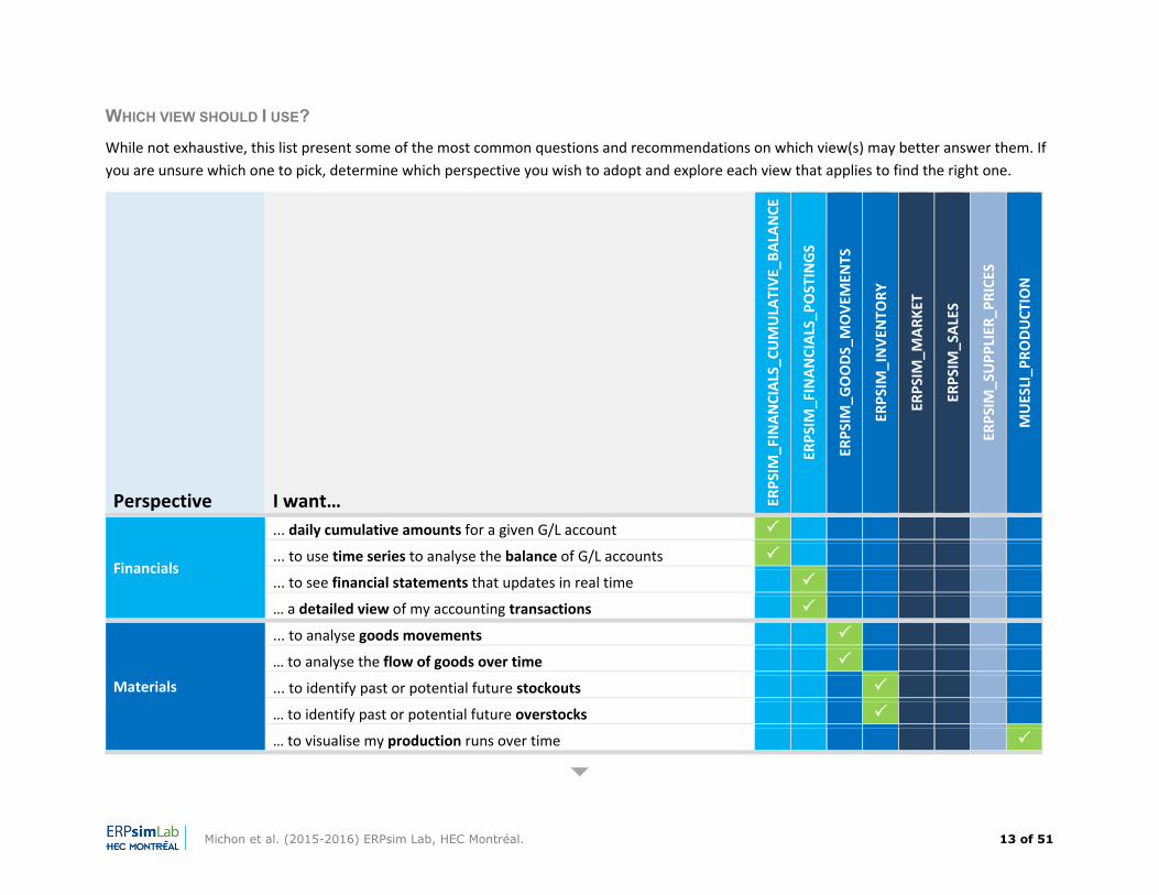
WHICH VIEW SHOULD I USE?

While not exhaustive, this list present some of the most common questions and recommendations on which view(s) may better answer them. If you are unsure which one to pick, determine which perspective you wish to adopt and explore each view that applies to find the right one.

Perspective I want… ERPSIM

_FINAN

CIAL

S_CU

MULA

TIVE

_BAL

ANCE

ERPSIM

_FINAN

CIAL

S_PO

STINGS

ERPSIM

_GOODS_MOVE

MEN

TS

ERPSIM

_INVE

NTO

RY

ERPSIM

_MAR

KET

ERPSIM

_SAL

ES

ERPSIM

_SUPP

LIER

_PRICE

S

MUESLI_P

RODUCT

ION

Financials

... daily cumulative amounts for a given G/L account � � � � � � �

... to use time series to analyse the balance of G/L accounts � � � � � � �

... to see financial statements that updates in real time � � � � � � �… a detailed view of my accounting transactions

Materials

... to analyse goods movements � � � � � � �… to analyse the flow of goods over time

... to identify past or potential future stockouts � � � � � � �… to identify past or potential future overstocks � � � � � � �… to visualise my production runs over time � � � � � � �


Perspective I want… ERPSIM

_FINAN

CIAL

S_CU

MULA

TIVE

_BAL

ANCE

ERPSIM

_FINAN

CIAL

S_PO

STINGS

ERPSIM

_GOODS_MOVE

MEN

TS

ERPSIM

_INVE

NTO

RY

ERPSIM

_MAR

KET

ERPSIM

_SAL

ES

ERPSIM

_SUPP

LIER

_PRICE

S

MUESLI_P

RODUCT

ION

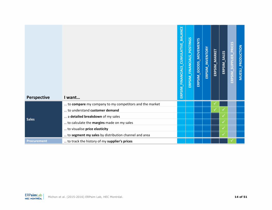
Sales

... to compare my company to my competitors and the market � � � � � � �

... to understand customer demand � � � � � �

... a detailed breakdown of my sales � � � � � � �… to calculate the margins made on my sales � � � � � � �… to visualise price elasticity � � � � � � �… to segment my sales by distribution channel and area

Procurement … to track the history of my supplier's prices � � � � � � �


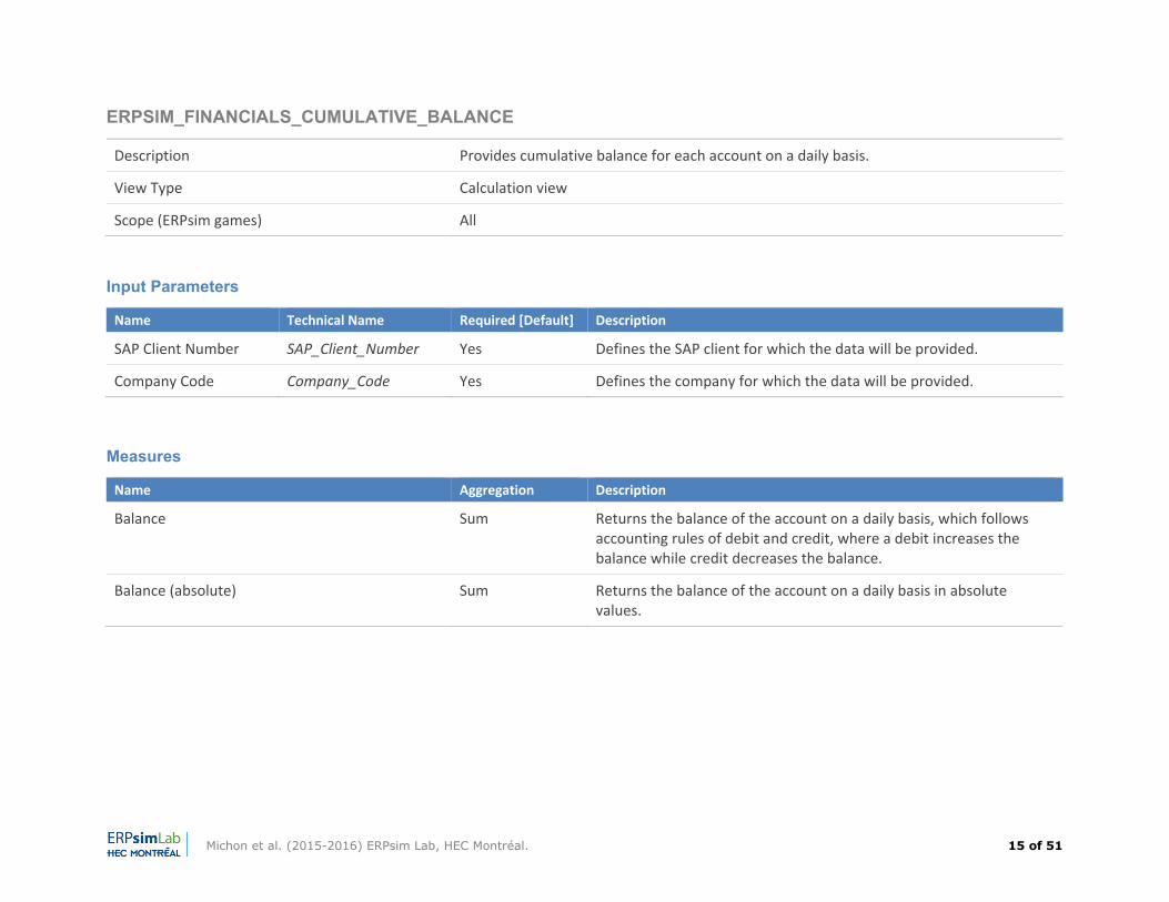
ERPSIM_FINANCIALS_CUMULATIVE_BALANCE

Description Provides cumulative balance for each account on a daily basis.

View Type Calculation view

Scope (ERPsim games) All

Input Parameters

Name Technical Name Required [Default] Description

SAP Client Number SAP_Client_Number Yes Defines the SAP client for which the data will be provided.

Company Code Company_Code Yes Defines the company for which the data will be provided.

Measures

Name Aggregation Description

Balance Sum Returns the balance of the account on a daily basis, which follows accounting rules of debit and credit, where a debit increases the balance while credit decreases the balance.

Balance (absolute) Sum Returns the balance of the account on a daily basis in absolute values.


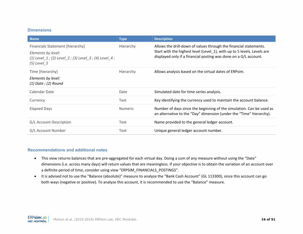
Dimensions

Name Type Description

Financials Statement [hierarchy]

Elements by level: (1) Level_1 ; (2) Level_2 ; (3) Level_3 ; (4) Level_4 ; (5) Level_5

Hierarchy Allows the drill‐down of values through the financial statements. Start with the highest level (Level_1), with up to 5 levels. Levels are displayed only if a financial posting was done on a G/L account.

Time [hierarchy]

Elements by level: (1) Date ; (2) Round

Hierarchy Allows analysis based on the virtual dates of ERPsim.

Calendar Date Date Simulated date for time series analysis.

Currency Text Key identifying the currency used to maintain the account balance.

Elapsed Days Numeric Number of days since the beginning of the simulation. Can be used as an alternative to the “Day” dimension (under the “Time” hierarchy).

G/L Account Description Text Name provided to the general ledger account.

G/L Account Number Text Unique general ledger account number.

Recommendations and additional notes

This view returns balances that are pre‐aggregated for each virtual day. Doing a sum of any measure without using the “Date” dimensions (i.e. across many days) will return values that are meaningless. If your objective is to obtain the variation of an account over a definite period of time, consider using view “ERPSIM_FINANCIALS_POSTINGS”.

It is advised not to use the “Balance (absolute)” measure to analyze the “Bank Cash Account” (GL 113300), since this account can go both ways (negative or positive). To analyze this account, it is recommended to use the “Balance” measure.


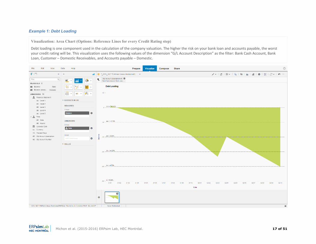
Example 1: Debt Loading

Visualization: Area Chart (Options: Reference Lines for every Credit Rating step)

Debt loading is one component used in the calculation of the company valuation. The higher the risk on your bank loan and accounts payable, the worst your credit rating will be. This visualization uses the following values of the dimension “G/L Account Description” as the filter: Bank Cash Account, Bank Loan, Customer – Domestic Receivables, and Accounts payable – Domestic.


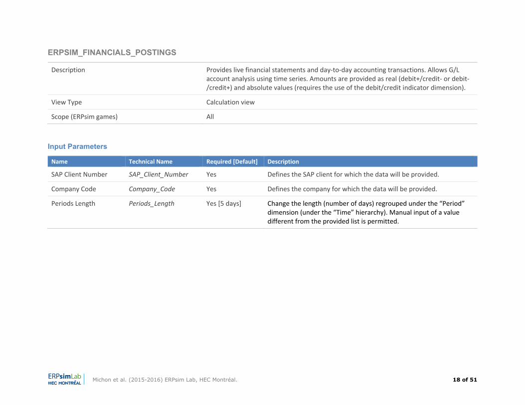
ERPSIM_FINANCIALS_POSTINGS

Description Provides live financial statements and day‐to‐day accounting transactions. Allows G/L account analysis using time series. Amounts are provided as real (debit+/credit‐ or debit‐/credit+) and absolute values (requires the use of the debit/credit indicator dimension).



Input Parameters




Periods Length Periods_Length Yes [5 days] Change the length (number of days) regrouped under the “Period” dimension (under the “Time” hierarchy). Manual input of a value different from the provided list is permitted.


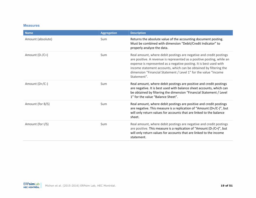
Measures


Amount (absolute) Sum Returns the absolute value of the accounting document posting. Must be combined with dimension “Debit/Credit Indicator” to properly analyze the data.

Amount (D‐/C+) Sum Real amount, where debit postings are negative and credit postings are positive. A revenue is represented as a positive posting, while an expense is represented as a negative posting. It is best used with income statement accounts, which can be obtained by filtering the dimension “Financial Statement / Level 1” for the value “Income Statement”.

Amount (D+/C‐) Sum Real amount, where debit postings are positive and credit postings are negative. It is best used with balance sheet accounts, which can be obtained by filtering the dimension “Financial Statement / Level 1” for the value “Balance Sheet”.

Amount (for B/S) Sum Real amount, where debit postings are positive and credit postings are negative. This measure is a replication of “Amount (D+/C‐)”, but will only return values for accounts that are linked to the balance sheet.

Amount (for I/S) Sum Real amount, where debit postings are negative and credit postings are positive. This measure is a replication of “Amount (D‐/C+)”, but will only return values for accounts that are linked to the income statement.


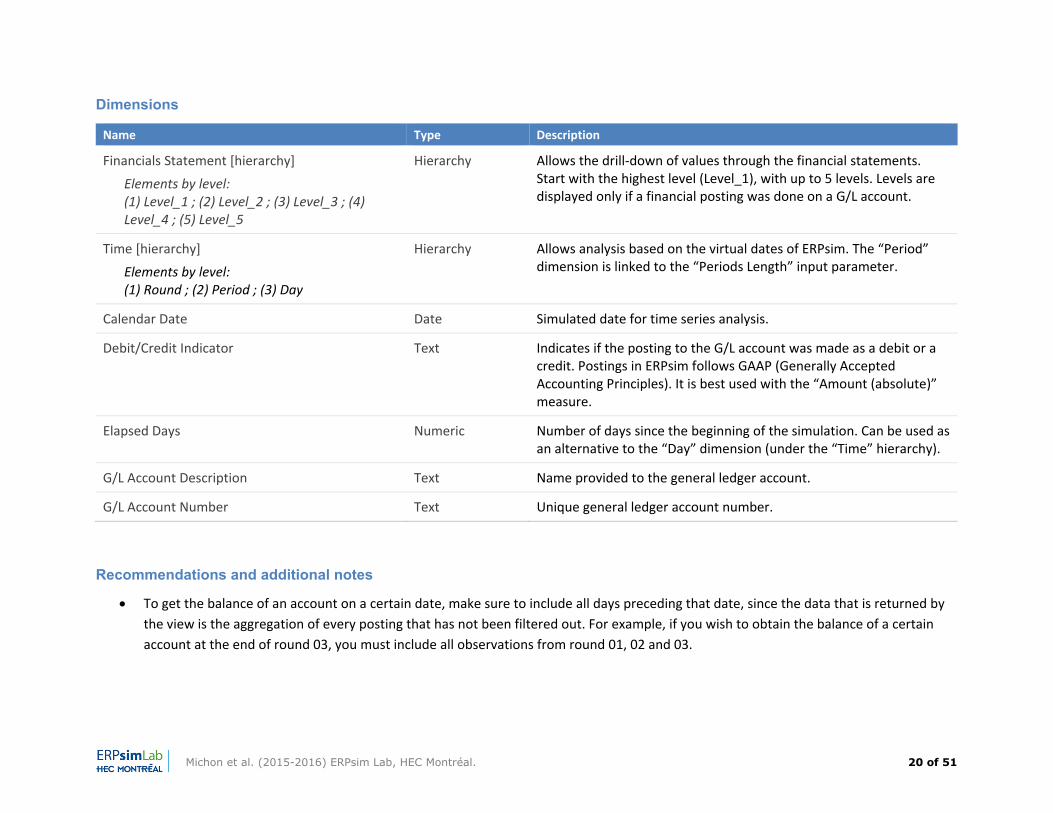
Dimensions


Financials Statement [hierarchy]

Elements by level: (1) Level_1 ; (2) Level_2 ; (3) Level_3 ; (4) Level_4 ; (5) Level_5

Hierarchy Allows the drill‐down of values through the financial statements. Start with the highest level (Level_1), with up to 5 levels. Levels are displayed only if a financial posting was done on a G/L account.

Time [hierarchy]

Elements by level: (1) Round ; (2) Period ; (3) Day

Hierarchy Allows analysis based on the virtual dates of ERPsim. The “Period” dimension is linked to the “Periods Length” input parameter.


Debit/Credit Indicator Text Indicates if the posting to the G/L account was made as a debit or a credit. Postings in ERPsim follows GAAP (Generally Accepted Accounting Principles). It is best used with the “Amount (absolute)” measure.


G/L Account Description Text Name provided to the general ledger account.

G/L Account Number Text Unique general ledger account number.


To get the balance of an account on a certain date, make sure to include all days preceding that date, since the data that is returned by the view is the aggregation of every posting that has not been filtered out. For example, if you wish to obtain the balance of a certain account at the end of round 03, you must include all observations from round 01, 02 and 03.


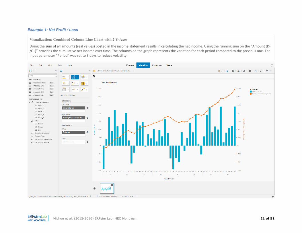
Example 1: Net Profit / Loss

Visualization: Combined Column Line Chart with 2 Y-Axes

Doing the sum of all amounts (real values) posted in the income statement results in calculating the net income. Using the running sum on the “Amount (D‐/C+)” provides the cumulative net income over time. The columns on the graph represents the variation for each period compared to the previous one. The input parameter “Period” was set to 5 days to reduce volatility.


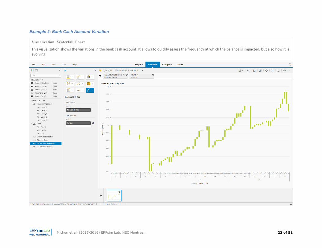
Example 2: Bank Cash Account Variation

Visualization: Waterfall Chart

This visualization shows the variations in the bank cash account. It allows to quickly assess the frequency at which the balance is impacted, but also how it is evolving.


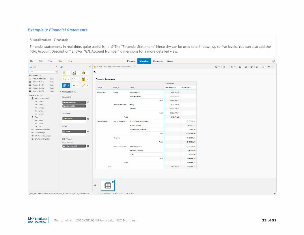
Example 3: Financial Statements

Visualization: Crosstab

Financial statements in real‐time, quite useful isn’t it? The “Financial Statement” hierarchy can be used to drill‐down up to five levels. You can also add the “G/L Account Description” and/or “G/L Account Number” dimensions for a more detailed view.


ERPSIM_GOODS_MOVEMENTS

Description Analyze material movements across your company.



Input Parameters





Measures


Quantity (absolute) Sum Returns the absolute quantity in the material posting. Combine with dimension “Debit/Credit Indicator” to properly analyze the data.

Quantity (real) Sum Returns the real value, where a debit increase the quantity, and a credit decrease the quantity.


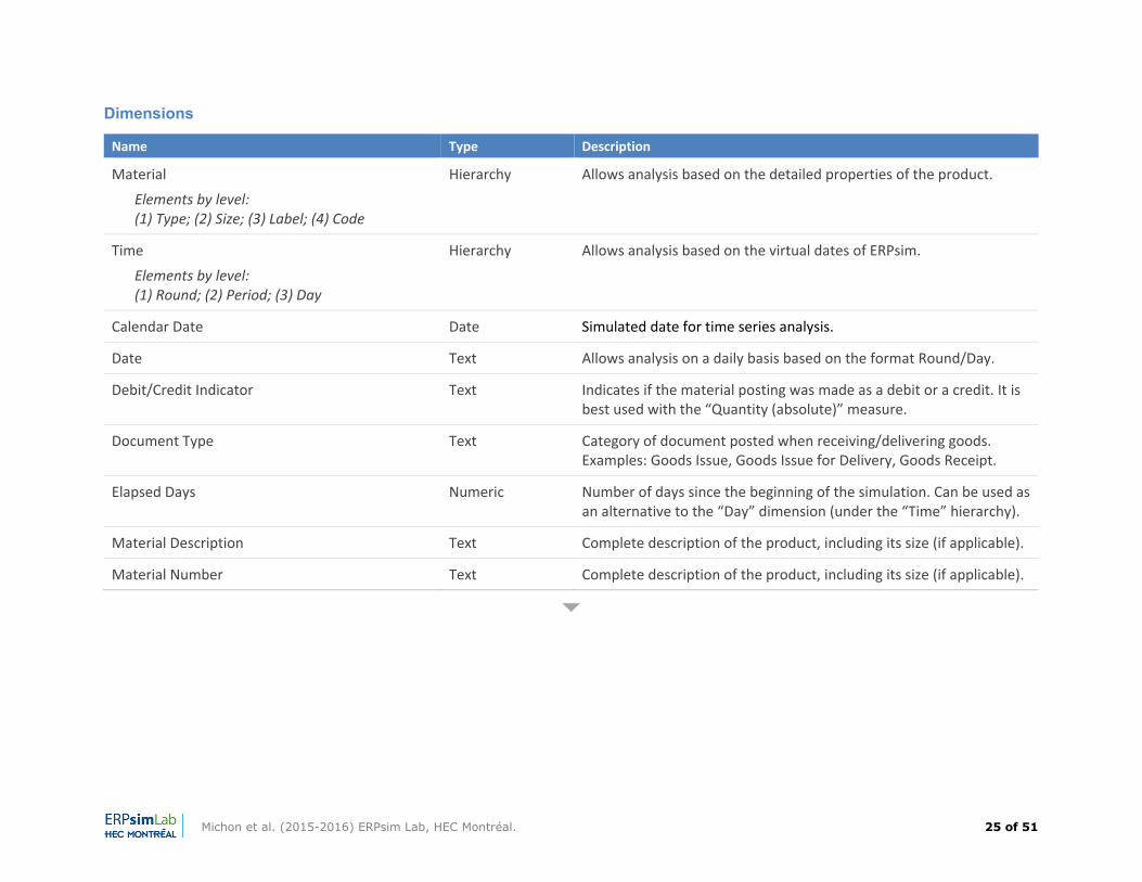
Dimensions


Material

Elements by level: (1) Type; (2) Size; (3) Label; (4) Code

Hierarchy Allows analysis based on the detailed properties of the product.

Time

Elements by level: (1) Round; (2) Period; (3) Day



Date Text Allows analysis on a daily basis based on the format Round/Day.

Debit/Credit Indicator Text Indicates if the material posting was made as a debit or a credit. It is best used with the “Quantity (absolute)” measure.

Document Type Text Category of document posted when receiving/delivering goods. Examples: Goods Issue, Goods Issue for Delivery, Goods Receipt.


Material Description Text Complete description of the product, including its size (if applicable).

Material Number Text Complete description of the product, including its size (if applicable).


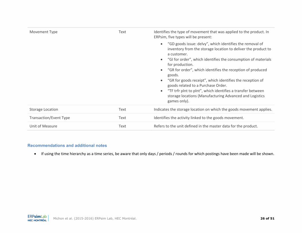
Movement Type Text Identifies the type of movement that was applied to the product. In ERPsim, five types will be present:

“GD goods issue: delvy”, which identifies the removal of inventory from the storage location to deliver the product to a customer.

“GI for order”, which identifies the consumption of materials for production.

“GR for order”, which identifies the reception of produced goods.

“GR for goods receipt”, which identifies the reception of goods related to a Purchase Order.

“TF trfr plnt to plnt”, which identifies a transfer between storage locations (Manufacturing Advanced and Logistics games only).

Storage Location Text Indicates the storage location on which the goods movement applies.

Transaction/Event Type Text Identifies the activity linked to the goods movement.

Unit of Measure Text Refers to the unit defined in the master data for the product.


If using the time hierarchy as a time series, be aware that only days / periods / rounds for which postings have been made will be shown.


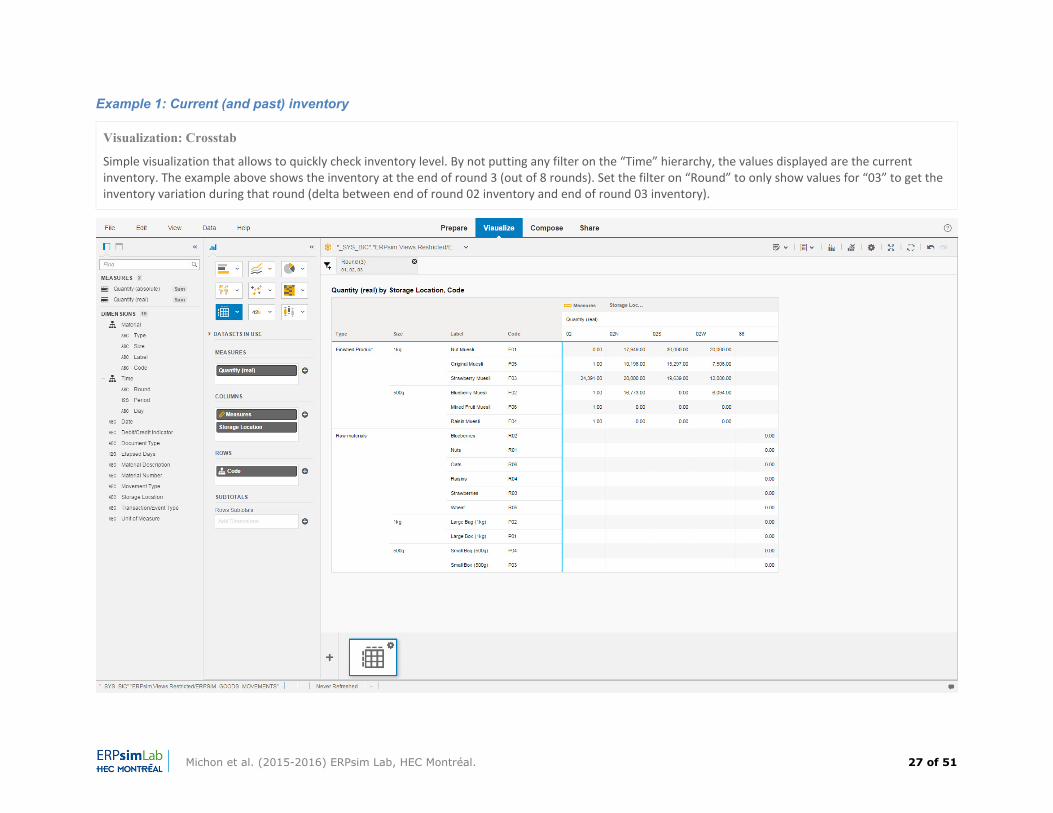
Example 1: Current (and past) inventory


Simple visualization that allows to quickly check inventory level. By not putting any filter on the “Time” hierarchy, the values displayed are the current inventory. The example above shows the inventory at the end of round 3 (out of 8 rounds). Set the filter on “Round” to only show values for “03” to get the inventory variation during that round (delta between end of round 02 inventory and end of round 03 inventory).


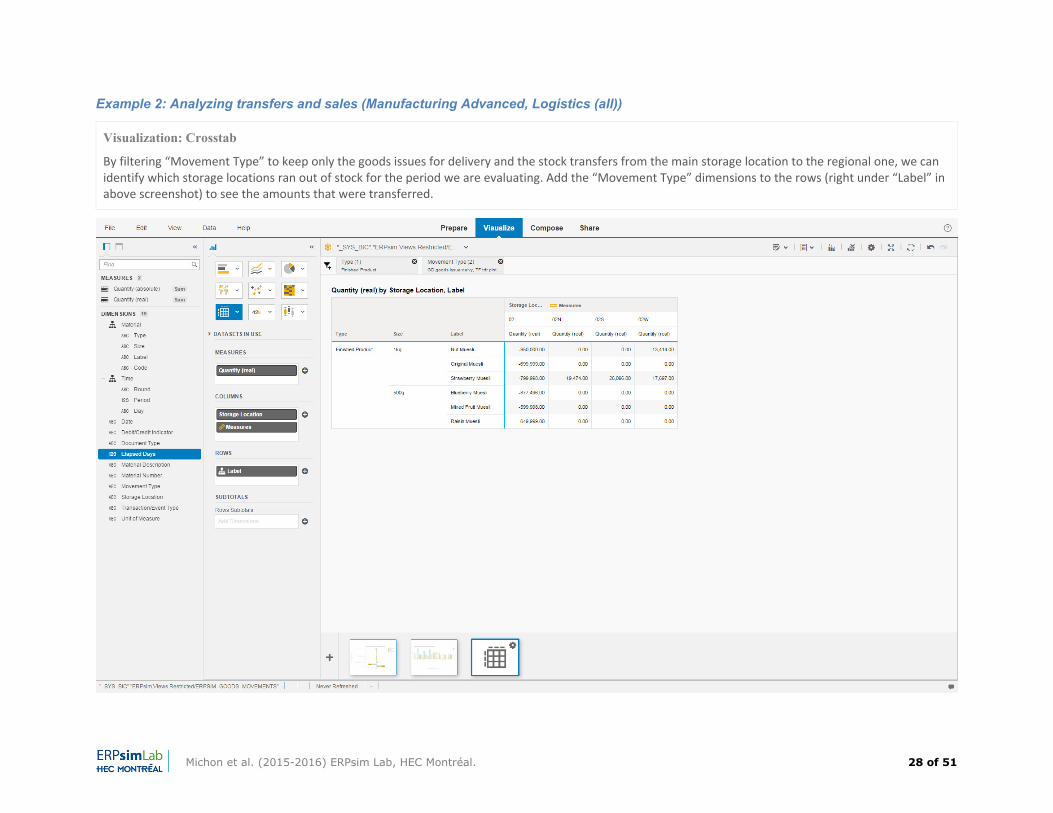
Example 2: Analyzing transfers and sales (Manufacturing Advanced, Logistics (all))


By filtering “Movement Type” to keep only the goods issues for delivery and the stock transfers from the main storage location to the regional one, we can identify which storage locations ran out of stock for the period we are evaluating. Add the “Movement Type” dimensions to the rows (right under “Label” in above screenshot) to see the amounts that were transferred.


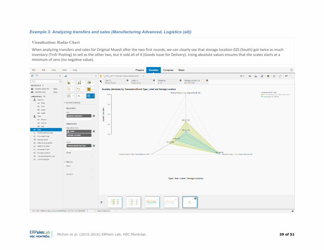
Example 3: Analyzing transfers and sales (Manufacturing Advanced, Logistics (all))

Visualization: Radar Chart

When analyzing transfers and sales for Original Muesli after the two first rounds, we can clearly see that storage location 02S (South) got twice as much inventory (Trsfr Posting) to sell as the other two, but it sold all of it (Goods Issue for Delivery). Using absolute values ensures that the scales starts at a minimum of zero (no negative value).


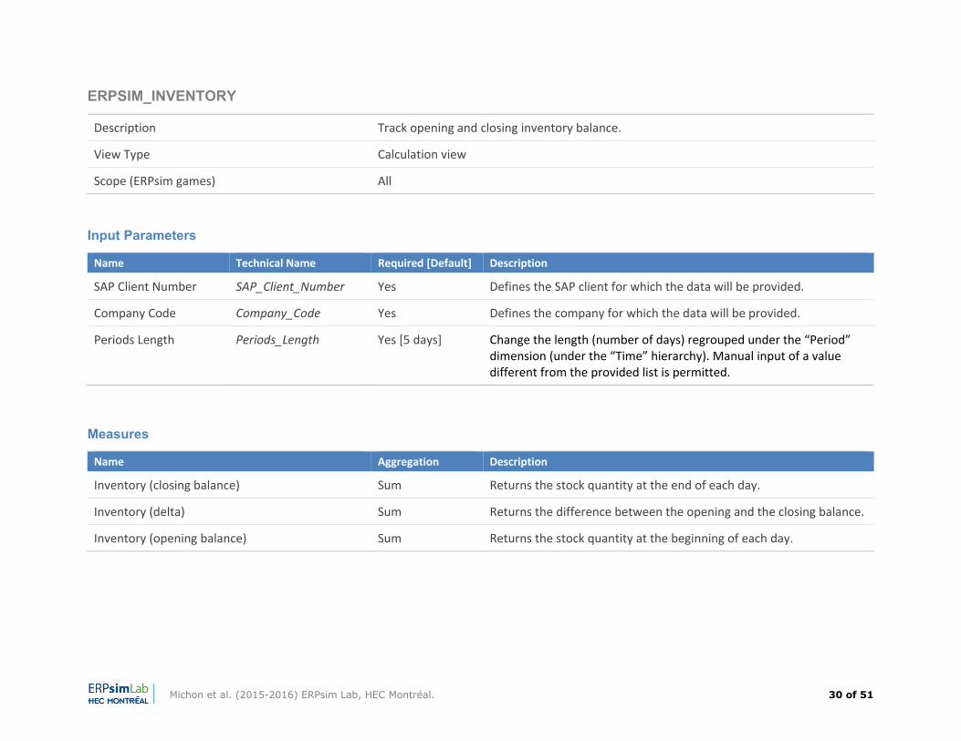
ERPSIM_INVENTORY

Description Track opening and closing inventory balance.



Input Parameters





Measures


Inventory (closing balance) Sum Returns the stock quantity at the end of each day.

Inventory (delta) Sum Returns the difference between the opening and the closing balance.

Inventory (opening balance) Sum Returns the stock quantity at the beginning of each day.


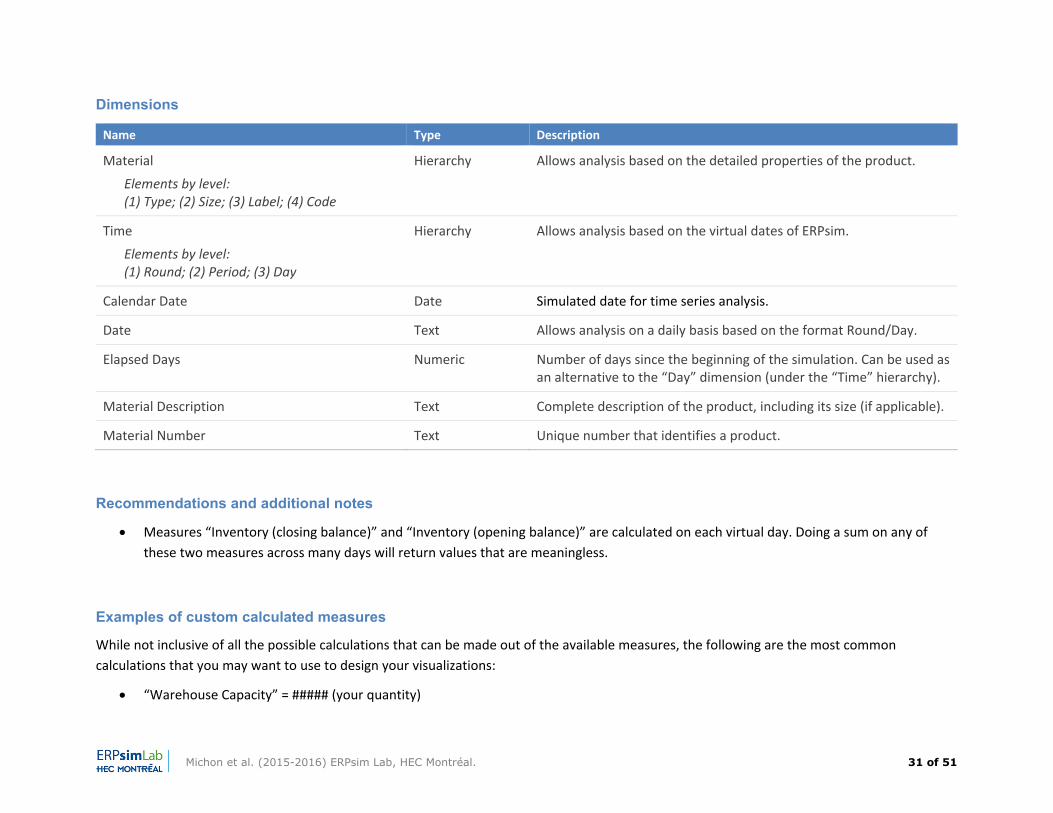
Dimensions


Material

Elements by level: (1) Type; (2) Size; (3) Label; (4) Code


Time




Date Text Allows analysis on a daily basis based on the format Round/Day.



Material Number Text Unique number that identifies a product.


Measures “Inventory (closing balance)” and “Inventory (opening balance)” are calculated on each virtual day. Doing a sum on any of these two measures across many days will return values that are meaningless.

Examples of custom calculated measures

While not inclusive of all the possible calculations that can be made out of the available measures, the following are the most common calculations that you may want to use to design your visualizations:

“Warehouse Capacity” = ##### (your quantity)


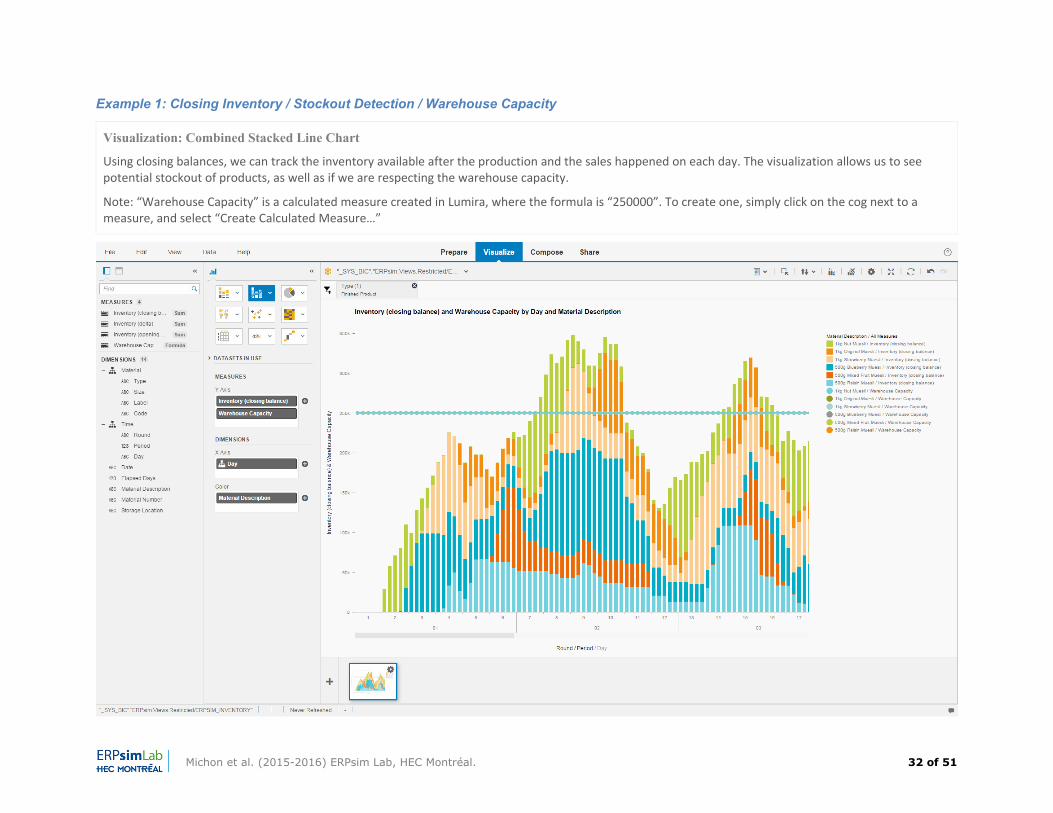
Example 1: Closing Inventory / Stockout Detection / Warehouse Capacity

Visualization: Combined Stacked Line Chart

Using closing balances, we can track the inventory available after the production and the sales happened on each day. The visualization allows us to see potential stockout of products, as well as if we are respecting the warehouse capacity.

Note: “Warehouse Capacity” is a calculated measure created in Lumira, where the formula is “250000”. To create one, simply click on the cog next to a measure, and select “Create Calculated Measure…”


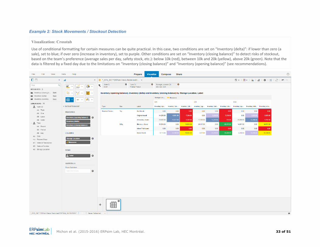
Example 2: Stock Movements / Stockout Detection


Use of conditional formatting for certain measures can be quite practical. In this case, two conditions are set on “Inventory (delta)”: if lower than zero (a sale), set to blue; if over zero (increase in inventory), set to purple. Other conditions are set on “Inventory (closing balance)” to detect risks of stockout, based on the team’s preference (average sales per day, safety stock, etc.): below 10k (red), between 10k and 20k (yellow), above 20k (green). Note that the data is filtered by a fixed day due to the limitations on “Inventory (closing balance)” and “Inventory (opening balance)” (see recommendations).


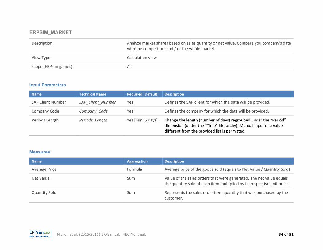
ERPSIM_MARKET

Description Analyze market shares based on sales quantity or net value. Compare you company's data with the competitors and / or the whole market.



Input Parameters




Periods Length Periods_Length Yes [min: 5 days] Change the length (number of days) regrouped under the “Period” dimension (under the “Time” hierarchy). Manual input of a value different from the provided list is permitted.

Measures


Average Price Formula Average price of the goods sold (equals to Net Value / Quantity Sold)

Net Value Sum Value of the sales orders that were generated. The net value equals the quantity sold of each item multiplied by its respective unit price.

Quantity Sold Sum Represents the sales order item quantity that was purchased by the customer.


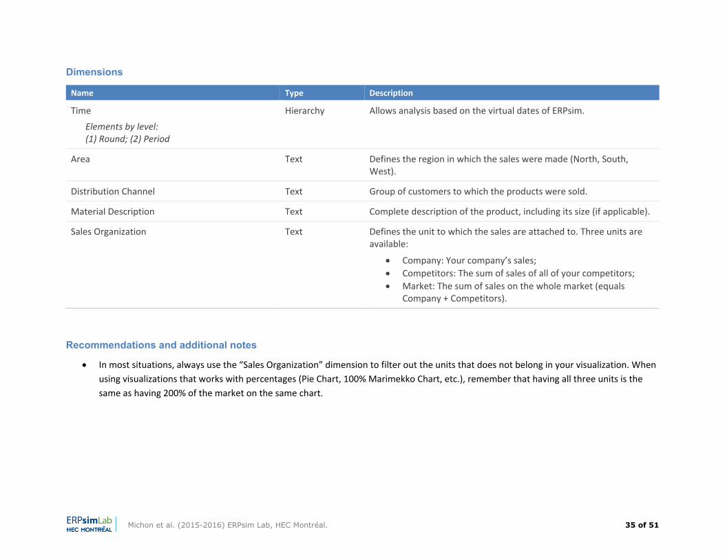
Dimensions


Time

Elements by level: (1) Round; (2) Period


Area Text Defines the region in which the sales were made (North, South, West).

Distribution Channel Text Group of customers to which the products were sold.


Sales Organization Text Defines the unit to which the sales are attached to. Three units are available:

Company: Your company’s sales; Competitors: The sum of sales of all of your competitors; Market: The sum of sales on the whole market (equals

Company + Competitors).


In most situations, always use the “Sales Organization” dimension to filter out the units that does not belong in your visualization. When using visualizations that works with percentages (Pie Chart, 100% Marimekko Chart, etc.), remember that having all three units is the same as having 200% of the market on the same chart.


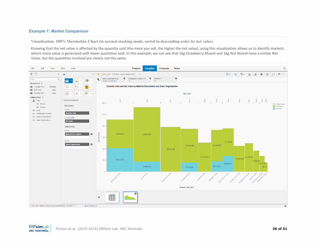
Example 1: Market Comparison

Visualization: 100% Marimekko Chart (in normal stacking mode, sorted in descending order by net value)

Knowing that the net value is affected by the quantity sold (the more you sell, the higher the net value), using this visualization allows us to identify markets where more value is generated with lower quantities sold. In this example, we can see that 1kg Strawberry Muesli and 1kg Nut Muesli have a similar Net Value, but the quantities involved are clearly not the same.


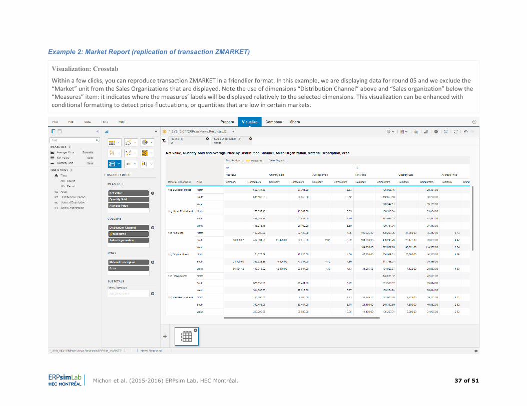
Example 2: Market Report (replication of transaction ZMARKET)


Within a few clicks, you can reproduce transaction ZMARKET in a friendlier format. In this example, we are displaying data for round 05 and we exclude the “Market” unit from the Sales Organizations that are displayed. Note the use of dimensions “Distribution Channel” above and “Sales organization” below the “Measures” item: it indicates where the measures’ labels will be displayed relatively to the selected dimensions. This visualization can be enhanced with conditional formatting to detect price fluctuations, or quantities that are low in certain markets.


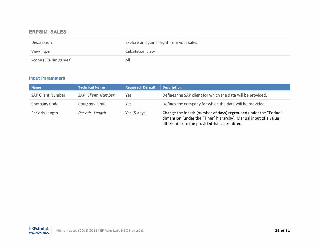
ERPSIM_SALES

Description Explore and gain insight from your sales.



Input Parameters






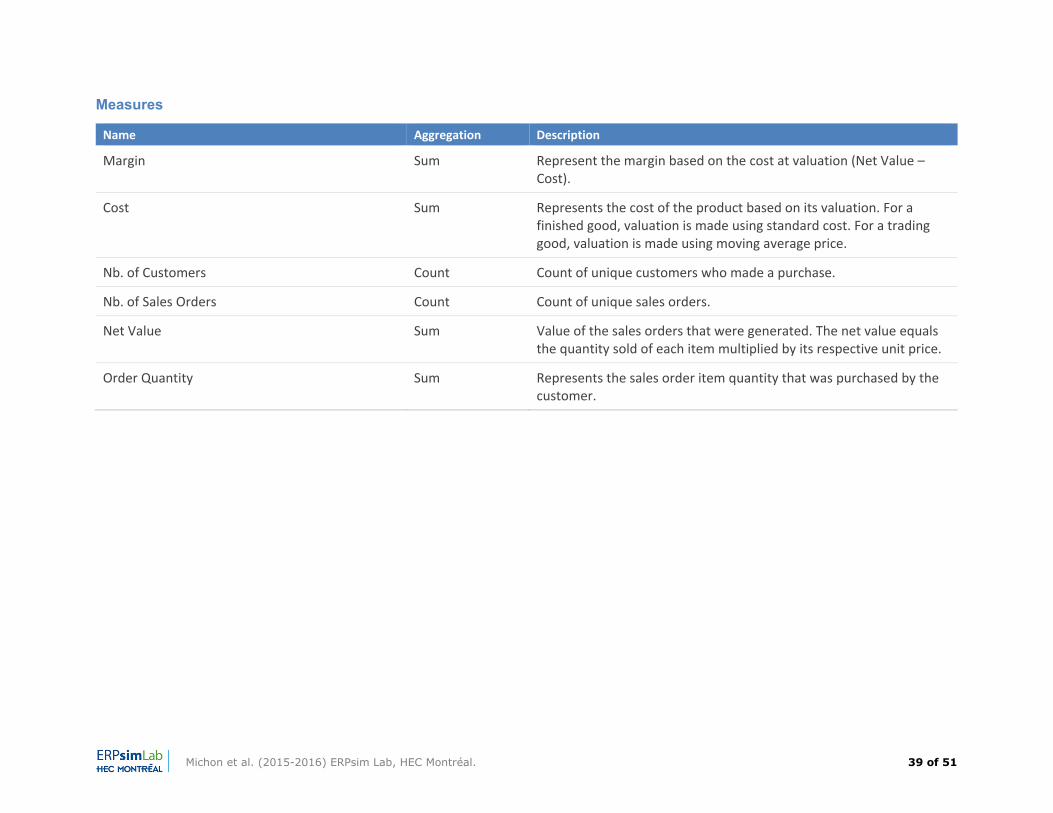
Measures


Margin Sum Represent the margin based on the cost at valuation (Net Value – Cost).

Cost Sum Represents the cost of the product based on its valuation. For a finished good, valuation is made using standard cost. For a trading good, valuation is made using moving average price.

Nb. of Customers Count Count of unique customers who made a purchase.

Nb. of Sales Orders Count Count of unique sales orders.

Net Value Sum Value of the sales orders that were generated. The net value equals the quantity sold of each item multiplied by its respective unit price.

Order Quantity Sum Represents the sales order item quantity that was purchased by the customer.


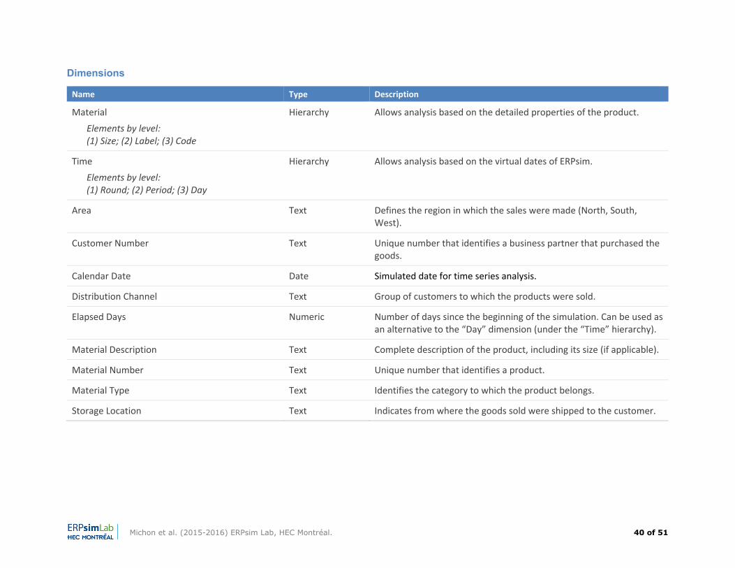
Dimensions


Material

Elements by level: (1) Size; (2) Label; (3) Code


Time



Area Text Defines the region in which the sales were made (North, South, West).

Customer Number Text Unique number that identifies a business partner that purchased the goods.


Distribution Channel Text Group of customers to which the products were sold.




Material Type Text Identifies the category to which the product belongs.

Storage Location Text Indicates from where the goods sold were shipped to the customer.



Measures "Nb. of Customers” and “Nb. of Sales Orders” can be used to calculate different ratios. For example, the average quantity sold per sales order can be obtained by dividing “Order Quantity” by “Nb. of Sales Orders”.

If using the time hierarchy as a time series, be aware that only days / periods / rounds for which sales have been recorder will be shown.

Examples of custom calculated measures

While not inclusive of all the possible calculations that can be made out of the available measures, the following are the most common calculations that you may want to use to design your visualizations:

“Average Order Quantity” = {Order Quantity} / {Nb. of Sales Order} “Average Unit Price” = {Net Value} / {Order Quantity} “Margin per Unit” = {Margin} / {Order Quantity}


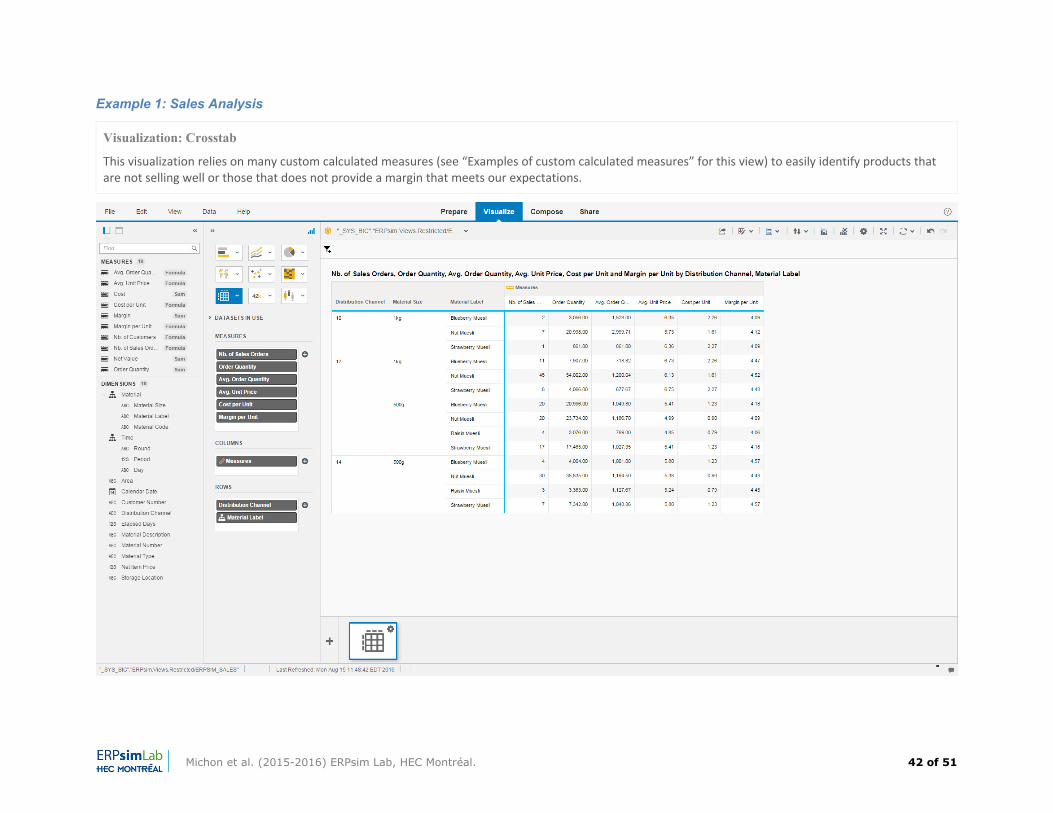
Example 1: Sales Analysis


This visualization relies on many custom calculated measures (see “Examples of custom calculated measures” for this view) to easily identify products that are not selling well or those that does not provide a margin that meets our expectations.


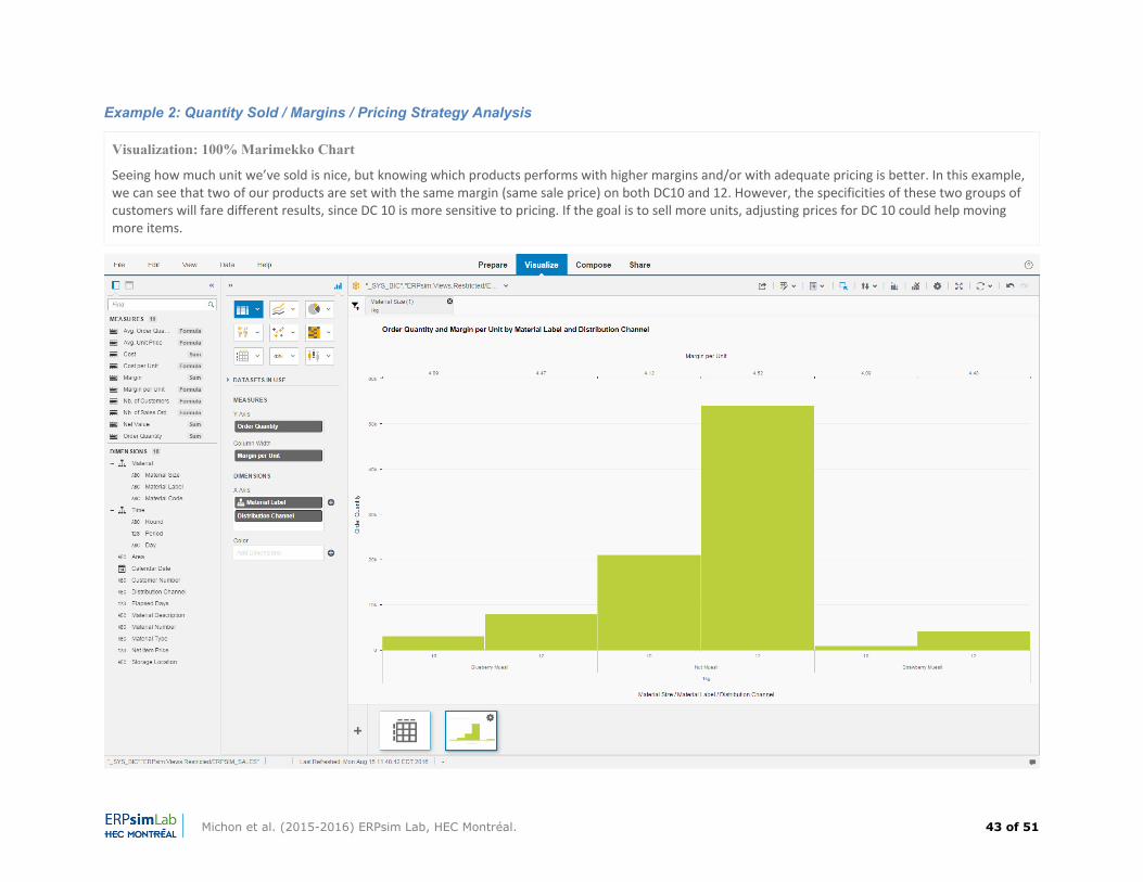
Example 2: Quantity Sold / Margins / Pricing Strategy Analysis

Visualization: 100% Marimekko Chart

Seeing how much unit we’ve sold is nice, but knowing which products performs with higher margins and/or with adequate pricing is better. In this example, we can see that two of our products are set with the same margin (same sale price) on both DC10 and 12. However, the specificities of these two groups of customers will fare different results, since DC 10 is more sensitive to pricing. If the goal is to sell more units, adjusting prices for DC 10 could help moving more items.


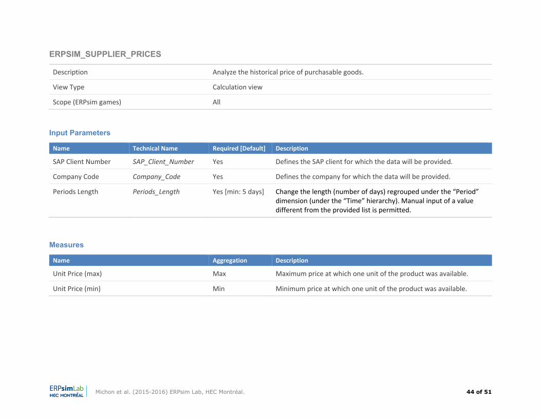
ERPSIM_SUPPLIER_PRICES

Description Analyze the historical price of purchasable goods.



Input Parameters




Periods Length Periods_Length Yes [min: 5 days] Change the length (number of days) regrouped under the “Period” dimension (under the “Time” hierarchy). Manual input of a value different from the provided list is permitted.

Measures


Unit Price (max) Max Maximum price at which one unit of the product was available.

Unit Price (min) Min Minimum price at which one unit of the product was available.


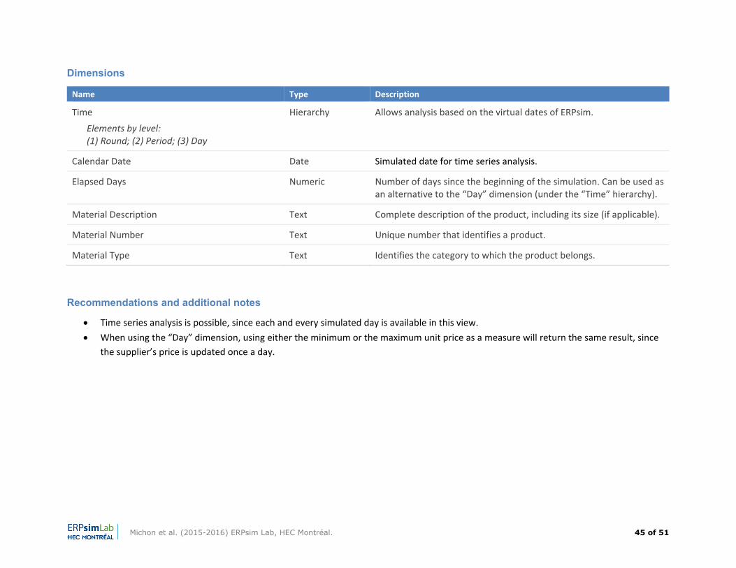
Dimensions


Time







Material Type Text Identifies the category to which the product belongs.


Time series analysis is possible, since each and every simulated day is available in this view. When using the “Day” dimension, using either the minimum or the maximum unit price as a measure will return the same result, since

the supplier’s price is updated once a day.


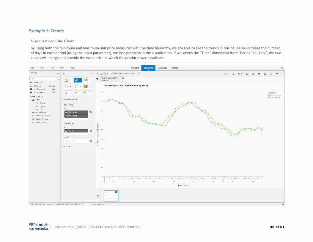
Example 1: Trends

Visualization: Line Chart

By using both the minimum and maximum unit price measures with the time hierarchy, we are able to see the trends in pricing. As we increase the number of days in each period (using the input parameter), we lose precision in the visualization. If we switch the “Time” dimension from “Period” to “Day”, the two curves will merge and provide the exact price at which the products were available.


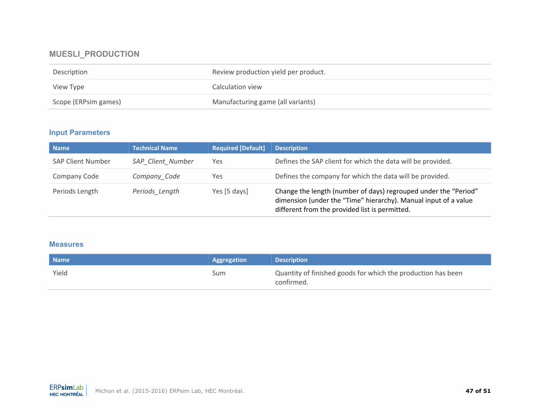
MUESLI_PRODUCTION

Description Review production yield per product.


Scope (ERPsim games) Manufacturing game (all variants)

Input Parameters





Measures


Yield Sum Quantity of finished goods for which the production has been confirmed.


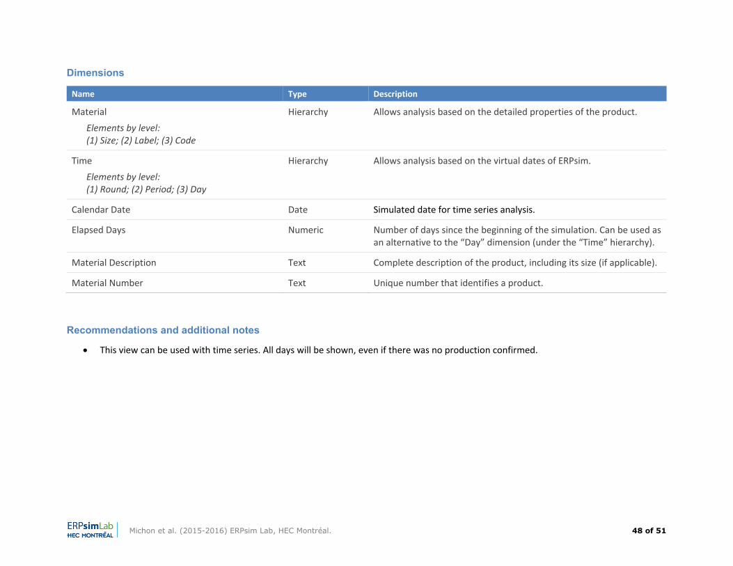
Dimensions


Material

Elements by level: (1) Size; (2) Label; (3) Code


Time








This view can be used with time series. All days will be shown, even if there was no production confirmed.


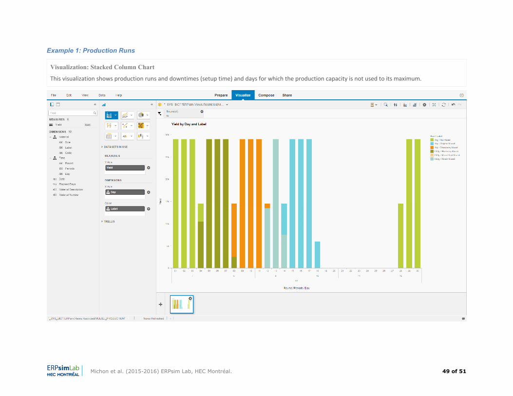
Example 1: Production Runs

Visualization: Stacked Column Chart

This visualization shows production runs and downtimes (setup time) and days for which the production capacity is not used to its maximum.


COPYRIGHT NOTICE

Document © Michon et al. (2015‐2016) ERPsim Lab, HEC Montréal.

ERPsim © Léger et al. (2004‐2016) ERPsim Lab, HEC Montréal. All rights reserved, including the right to reproduce this book or portions thereof in any form.

Copying or distributing in print or electronic forms without written permission of HEC Montréal is prohibited.

For information contact ERPsim Lab, HEC Montréal, 3000 Chemin de la Côte Sainte‐Catherine, Montréal (Québec), Canada, H3T 2A7, or visit https://erpsim.hec.ca

For academic use only. For information about commercial use, please visit http://www.batonsimulations.com/

This document contains references to the products of SAP SE, Dietmar‐Hopp‐Allee 16, 69190 Walldorf, Germany. The names of these products are registered and/or unregistered trademarks of SAP SE. SAP SE is neither the author nor the publisher of this book and is not responsible for its content.

Made in Canada


DOCUMENT REVISION CONTROL

Revision Draft Date Author/Reviewer Comments

1 ‐ 2015‐03‐08 Jean‐François Michon Document created.

1 1 2015‐08‐20 Hikmath Yemissi Eyitayo Initial draft of the structure of each view.

1 2 2015‐09‐07 Jean‐François Michon Improvement of the description of each item within the views’ structure.

1 3 2015‐09‐15 Hikmath Yemissi Eyitayo Update of Lumira’s examples views.

1 4 2015‐09‐17 Jean‐François Michon Major redaction work.

2 ‐ 2015‐09‐24 Jean‐François Michon Released.

2 1 2015‐09‐25 Jean‐François Michon Minor updates to text and layout.

2 2 2015‐10‐01 Jean‐François Michon Minor layout updates. Fixes to introduction.

2 3 2015‐10‐02 Jean‐François Michon Section title revision.

2 4 2015‐11‐30 Jean‐François Michon Added: New view (ERPSIM_SUPPLIER_PRICES) Minor revisions to the text.

2 5 2016‐02‐17 Jean‐François Michon Revision of the introduction for “PART ONE: USING SAP HANA VIEWS FOR ERPSIM” Minor updates to text.

3 ‐ 2016‐08‐12 Jean‐François Michon Released.

3 1 2016‐08‐12 Jean‐François Michon Updated views’ name according to latest release. Reviewed dimensions and measures, as well as the example, for view ERPSIM_FINANCIALS_CUMULATIVE_BALANCE. Added the Calendar Date dimension to all the views that has it.

4 ‐ 2016‐08‐15 Jean‐François Michon Released

Date post:	16-Jun-2018
Category:	Documents
Upload:	vanphuc
View:	236 times
Download:	0 times

ERPsim for SAP HANA - Reference Guide -...

Documents