Eurographics Symposium on Geometry Processing (2006)Konrad Polthier, Alla Sheffer (Editors)

Error Bounds and Optimal Neighborhoods for MLSApproximation

Yaron Lipman Daniel Cohen-Or David Levin

Tel-Aviv University

Abstract

In recent years, the moving least-square (MLS) method has been extensively studied for approximation and recon-struction of surfaces. The MLS method involves local weighted least-squares polynomial approximations, usinga fast decaying weight function. The local approximating polynomial may be used for approximating the under-lying function or its derivatives. In this paper we consider locally supported weight functions, and we addressthe problem of the optimal choice of the support size. We introduce an error formula for the MLS approximationprocess which leads us to developing two tools: One is a tight error bound independent of the data. The secondis a data dependent approximation to the error function of the MLS approximation. Furthermore, we provide ageneralization to the above in the presence of noise. Based on the above bounds, we develop an algorithm toselect an optimal support size of the weight function for the MLS procedure. Several applications such as differen-tial quantities estimation and up-sampling of point clouds are presented. We demonstrate by experiments that ourapproach outperforms the heuristic choice of support size in approximation quality and stability.

Categories and Subject Descriptors(according to ACM CCS): I.3.3 [Computer Graphics]: Surface approximation,Point clouds, Meshes, Differential quantities estimation

1. Introduction

A fundamental problem in surface processing is the recon-struction of a surface or estimating its differential quantitiesfrom scattered (sometimes noisy) point data [HDD∗92]. Acommon approximation approach is fitting local polynomi-als, explicitly [ABCO∗01], or implicitly [OBA∗03], to ap-proximate the surface locally. This approach can be realizedby the moving least-squares (MLS) method, where, for eachpointx, a polynomial is fitted, in the least-squares sense, us-ing neighboring pointsxi . This technique works well assum-ing that the surface is smooth enough [Lev98,Wen01]. Thelocal polynomial fitting enables up and down sampling of thesurface [ABCO∗01], estimating differential quantities suchas normal or curvature data [CP05], and performing othersurface processing operations [PKKG03].

In recent years, the MLS technique has gained much pop-ularity, and the method is now well studied. However, properchoice of neighboring pointsxi to be used in the approx-imation still remains an important open problem. Appar-ently, there is a large degree of freedom in choosing the

points participating in the approximation since the numberof data points is usually very large, while the degree ofpolynomial is usually very small. Naturally, one would liketo make use of these large degrees of freedom to achievethe “best” approximating polynomial. Several researchers[ABCO∗01, PGK02, PKKG03] have used different heuris-tic approaches, such as using a neighborhood proportionalto the local sampling density measured via the radius of theball containing theK nearest neighbors, or using Voronoi tri-angulation [FR01] to choose the neighboring points. In thispaper, we compare a heuristic method in the spirit of theseapproaches with a new approach based on error analysis.

Since the problem of choosing the points to be used inthe approximation is closely related to multivariate inter-polation, it is known that the choice of the points dependson the geometry of the points, and not only their num-ber, as in the sampling density based approaches. How-ever, the geometric configuration of points which admits astable interpolation/approximation problem is a hard prob-lem in the field of multivariate polynomial approximation[Bos91, SX95, GS00]. Loosely speaking, a ‘stable’ points’

c© The Eurographics Association 2006.

Y. Lipman & D. Cohen-Or & D. Levin / Error Bounds and Optimal Neighborhoods for MLS Approximation

(a) (b)

(c) (d)

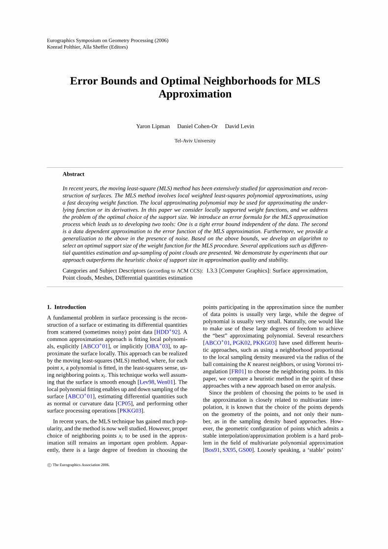
Figure 1: Resampling of a noisy surface. A patch of the dragonmodel (a) with additional white noise (b) is resampled with twomethods: Using the local density (heuristic) to determine the lo-cal neighborhood yields some noticeable artifacts (c). The proposedmethod, assuming the maximal value of the noise is known, faithfullyreconstruct the surface.

configuration is such that is ‘far’ from a degenerate pointconfiguration, where a degenerate point configuration lieson an algebraic curve of the dimension of the interpolationspace.

Preliminary example. Consider the pointsXh =h(cosj2π/6,sin j2π/6), j = 0,1, ..,5. X forms a degen-erate point configuration for bi-variate quadratic interpola-tion. Although this point set seems nicely distributed around(0,0), quadratic interpolation cannot be used for approxi-mation at(0,0), no matter how small we takeh. This canbe seen by taking, for example, the values associated withxi ∈ Xh to be zeros and noting that bothf1(x) ≡ 0 andf2(x) = (h2− x2

1− x22)/h3 solve the interpolation problem,

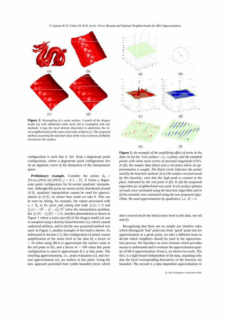
but | f1(0)− f2(0)| ∼ 1/h. Another phenomenon is shown inFigure1 where a noisy part (b) of the dragon model (a) wasre-sampled using a density based heuristic (c), which causedundesired artifacts, and in (d) the new proposed method wasused. In Figure2, another example of this kind is shown. Aselaborated in Section3.5, this configuration of points causesamplification of the noise level in the data by a factor of∼ 10 when using MLS to approximate the surface value atthe red point in (b), and a factor of∼ 100 when this pointconfiguration is used to approximate∂x f at that point. Theresulting approximations, i.e., point evaluation (c), and nor-mal approximation (e), are useless at this point. Using thenew approach presented here yields bounded errors which

(a) (b)

(c) (d)

(e) (f)

Figure 2: An example of the amplifying effect of noise in thedata. In (a) the ‘true surface’, i.e., a plane, and the sampledpoints with white noise errors of maximal magnitude0.015.In (b), the sample data (blue) and a red point where an ap-proximation is sought. The black circle indicates the pointsused by the heuristic method. In (c) the surface reconstructedby this heuristic, note that the high peak is created at theplace indicated by the red point in (b). In (d) the proposedalgorithm for neighborhood was used. In (e) surface (plane)normals were estimated using the heuristic algorithm and in(f) the normals were estimated using the new proposed algo-rithm. We used approximation by quadratics, i.e., N= 2.

don’t exceed much the initial noise level in the data, see (d)and (f).

Recognizing that there are no simple nor intuitive ruleswhich distinguish ‘bad’ point sets from ‘good’ point sets forapproximation at a given point, we take a different route todecide which neighbors should be used in the approxima-tion process: We introduce an error formula which providesmeans to understand and to evaluate the approximation qual-ity of MLS approximation. From it, we derive two tools. Thefirst, is a tight bound independent of the data, assuming onlythat the local corresponding derivatives of the function arebounded. The second is a data dependent approximation to

c© The Eurographics Association 2006.

Y. Lipman & D. Cohen-Or & D. Levin / Error Bounds and Optimal Neighborhoods for MLS Approximation

the error function of the MLS interpolant. We examine thepractical usage of these tools and compare them to a care-fully chosen heuristic method.

Based on the above bounds, we develop an algorithm toselect an optimal radial neighborhood for the MLS proce-dure. Loosely speaking, since the underlying surface fromwhich the sampled points are taken is unknown, the opti-mality of the chosen neighborhoods is in the sense of theapproximation error having the lowest error bound.

MLS approximations are used in a variety of cases, but theproblem is always reduced to the functional case, by definingsome parameter domain [Lev03, ABCO∗01]. Thus, for theerror analysis, it is enough to consider the functional case.

We develop the various theoretical error terms and boundsin Section3, and based on these results, in Section4, weintroduce an algorithm for selecting the optimal neighbor-hood. In Section5 we derive a heuristic rule which we usefor comparison. In the following section, we briefly describethe MLS technique, and define the terms and notation to beused in the paper. In Section6 we present some numericalexperiments, and in Section7 we conclude.

2. Background

Surfaces or 2-manifolds embedded inIR3 are most com-monly represented by a set of spacial points, with neighbor-ing relations (meshes) or without (point clouds). A commonway to estimate the value of the surface in a new point, orto estimate differential quantities of the surface at any point,is by fitting a local polynomial and extracting it’s value orderivatives.

In order to reduce the problem to the functional case alocal parameter plane is constructed, and the local polyno-mial is defined over this parameter space. Eventually, oneends up with the problem of fitting a polynomialp ∈ Π,where Π is some polynomial subspace, given data points(xi , f (xi)) ∈ Ω× IR, i = 1, .., I , whereΩ is a domain inIRd.The goal is to approximate a functionalLx at a pointx∈ Ω,whereLx can be a function evaluation atx or a derivativeevaluation, e.g.,Lx( f ) = f (x) or Lx( f ) = (∂xy f )(x). A com-mon way to do it is by fitting the polynomial locally in theleast-squares sense:

min

I

∑i=1

( f (xi)− p(xi))2 w(‖xi −x‖) , p∈ Π

, (1)

wherew(r) is a radial weight function. When the minimizerpolynomial p is achieved, the approximation functionalLx

is applied to it to form the approximation

Lx( f )≈ Lx(p). (2)

As showed in [Lev98],

Lx(p) =I

∑i=1

ai f (xi),

whereai are the solution to the constrained quadratic mini-mization problem

minI

∑i=1

w(‖x−xi‖)−1|ai |2 s.t.I

∑i=1

ai p(xi) = p(x), ∀p∈ Π

.

The weight functionw is usually chosen to ensure fast decayof the magnitude of theai for points distant from the evalu-ation pointx. The decay rate is heuristically chosen to be asfast as possible while keeping enough points in the signifi-cant weights area to keep the problem well-posed. Further-more, a smooth weight function implies smooth approxima-tion. In this paper we have chosen to use the weight functionof finite support [Lev98], w(r) = wh(r), where

wh(r) = e− r2

(h−r)2 χ[0,h)(r). (3)

The main objective of this paper is to present an algorithmfor choosing the support sizeh which best assures a mini-mal approximation error using the procedure (1)-(2). This isaccomplished in two independent ways: First by minimiz-ing a novel, tight, local error bound formula. This procedurealso supplies a bound on the error which is achieved in theapproximation process, given that a bound on local corre-sponding derivatives off is known. Second, a novel approxi-mation of the error in the MLS approximation is constructed,and the best support sizeh is chosen as before. The lattergenerally performs better than the former.

3. Error analysis3.1. Settings

The settings of the problem consists of a data set(xi , f (xi)),X = xiI

i=1 ⊂ Ω ⊂ IRd, sampled from a smooth functionf ∈ Ck(Ω), and another pointx where an approximationLx f = Dα f (x), whereDα = ∂α1

x(1) · ... ·∂αd

x(d) , is sought. Denoteby N the degree of the polynomials used as the approxima-tion space.J =

(N+dd

)is the dimension of the spaceΠN of d-

variate polynomial of degreeN. Also definep1, p2, ..., pJ ∈Π to be the standard basis ofΠN shifted to x, that is,(· − x)α|α|≤N, where we use the multi-index notationα = (α1, ...,αd), α! = α1! · ... ·αd!, |α|= α1 + ...+αd, andfor x = (x(1), ...,x(d)) xα = (x(1))α1...(x(d))αd . We also de-fine the generalized Vandermonde matrixE by Ei,β = pβ(xi),i = 1, .., I , |β| ≤ N.

Denote the subsetXh = X∩Bh(x), whereBh(x) denotes aball of radiush with centerx, and letI = |Xh|, the numberof data points inBh(x). Then, for a fixedh, we define theapproximationDα f (x)≈Dα p(x), wherep∈ΠN, is definedby (1), andw = wh defined by (3).

Let us introduce some test functions. The first one is takenfrom [Fra82],

F1 =304

e−(9x+5)2+(9y+5)2

16 +304

e−(9x+11)2

196 −9y+11

20 (4)

+102

e−(9x−5)2+(9y+3)2

16 − 105

e−(9x+1)2+(9y−5)2

4 .

c© The Eurographics Association 2006.

Y. Lipman & D. Cohen-Or & D. Levin / Error Bounds and Optimal Neighborhoods for MLS Approximation

(a) (b) (c)

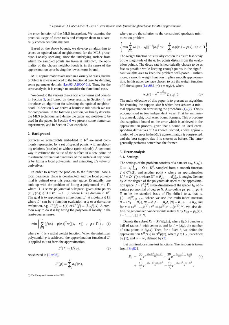
Figure 3: The test function used in the paper. (a) is the graph ofF1, (b) of F2 and (c) of F3.

F2 = 0.3cos(8x)sin(6y)+e−x2−y2

. (5)

F3 = cos(20x). (6)

In Figure3, we plotted the graphs of these test functions.These functions were selected since they seem to representwell several smooth surface types:F1 is a standard test func-tion and has been used in numerous papers.F2 has interest-ing ’details’, andF3 is an anisotropic surface with very highderivatives.

3.2. Pointwise error in the MLS approximation

In this section we lay out the formula for the error in theMLS approximation which forms the basis for all latter de-velopments in the paper:

Theorem 3.1Denote byp the fitted polynomial defined by(1) to the data(Xh, f (Xh))⊂Ω× IR, sampled from a smoothfunction f ∈CN+1(Ω), then forx∈ Ω,

R(x) = Dα p(x)−Dα f (x) = (7)

α!(N+1)! ∑

i,νDν f (ηi(xi −x)+x)(xi −x)ν det

(EtWEα←ei

)det(EtWE)

where∑i,ν stands for∑|ν|=N+1 ∑Ii=1, 0≤ ηi ≤ 1, andE is

the Vandermonde matrixEi,β = pβ(xi). Eα←ei denotes thematrix E where theα column is replaced by the standardbasis vectorei = δ j,i . The weight matrixW is defined byW = diag(wh(‖x1−x‖), ...,wh(‖xI −x‖)).

Proof. The proof relies on the polynomial reproduction prop-erty of the Least-Squares method and is based upon localTaylor expansions as approximations off .

First, w.l.o.g, we may assumex = 0. Denote byp1, ..., pJthe standard basis of the multivariate polynomials of degree≤N, that ispα(x) = xα, |α| ≤N. Next, writingp= ∑β cβ pβ,leads to

Dα p(0) = ∑β

cβDα pβ(0) = ∑β

cβα!δα,β = α!cα.

The multivariate Vandermonde matrixE is ordered by themulti-indexβ, i.e.,Ei,β = pβ(xi), as we do also for the vectorc = cβ|β|≤N of the unknown coefficients. The fitted poly-nomial p is then defined as the solution in the least-squares

sense. That is,c satisfies the normal equations:

EtWEc= EtWF. (8)

Using Taylor expansion,

f (xi) = ∑|ν|≤N

Dν f (0)ν!

xνi +

1(N+1)! ∑

|ν|=N+1

Dν f (ηixi)xνi ,

where 1≤ ηi ≤ ν. Hence, the vectorF can be written as

F = ∑|ν|≤N

Dν f (0)ν!

Eν +1

(N+1)! ∑|ν|=N+1

QνEν,

where Qν = diag(Dν f (η1x1), ...,Dν f (ηI xI )), and Eν de-notes theν column vector of matrixE. Then, For the solutionof (8) we have,

cν =Dν f (0)

ν!+

1(N+1)!

(∑

|ν|=N+1

(EtWE)−1EtWQνEν

)ν

.

Next, EtWQνEν = ∑Ii=1(E

tW)iDν f (ηixi)pν(xi), with

pν(xi) = xνi , and by Cramer’s rule and the linearity of the

determinant((EtWE)−1EtWQνEν

)ν

=

I

∑i=1

Dν f (ηixi)xνi

det(EtWEν←ei )det(EtWE)

.

Finally we get forν = α, α!cα−Dα f (0) =

α!(N+1)! ∑

|ν|=N+1

I

∑i=1

Dν f (ηixi)xνi

det(EtWEν←ei )det(EtWE)

,

where|ν|= N+1 andi = 1, ..,n.

Corollary 3.1 Denote byp the fitted polynomial defined by(1) to the data(Xh, f (Xh)) ∈ Ω ⊂ IRd × IR, sampled from asmooth functionf ∈CN+1(Ω), then the following is atighterror bound,

|R(x)| ≤ α!C(N+1)! ∑

i,ν|xi −x|ν

∣∣∣∣∣det(EtW(E)α←ei

)det(EtWE)

∣∣∣∣∣ ,whereC is the bound: max|ν|=N+1,x∈Ω |Dν f (x)| ≤C.

3.3. Data Independent Bound

For a given support sizeh, an error bound for the polynomialfitting procedure based on the dataXh can be calculated viathe tight bound in Corollary (3.1). We define the boundingfunctionBα by

Bα = Bα(x,Xh) =α!

(N+1)! ∑β,i

|xi −x|β |det(EtWEα←ei )||det(EtWE)| ,

(9)where, as before,∑i,β is a short notation for∑|ν|=N+1 ∑I

i=1.

>From the computational point of view, in order to com-

pute (9), we note thatdet(EtWEα←ei )

det(EtWE) is theα coordinate of

c© The Eurographics Association 2006.

Y. Lipman & D. Cohen-Or & D. Levin / Error Bounds and Optimal Neighborhoods for MLS Approximation

the solution to the linear system:

EtWEc= (EtW)i ,

where (EtW)i denotes thei-th column of matrix EtW.Therefore, in the calculation of (9), one should calculate thesolutionV to ETWEV= EtW, and then set

Vα,i =det(EtWEα←ei )

det(EtWE). (10)

Then formula (9) reduces to,

Bα(x,Xh) =α!

(N+1)! ∑β,i

|xi −x|β|Vα,i |. (11)

3.4. Data dependent error approximation

In this section we construct a data dependent approxima-tion to the error function in the MLS approximation forf ∈ CN+2(Ω). This error approximation uses the knownvalues at the pointsXh in order to better approximate theerror in the approximation (7). In particular we note thatDν f (ηi(xi−x)+x) = Dν f (x)+O(h), for |ν|= N+1, whereh is the support size used. Therefore, Eq. (7) can be writtenas:

R(x) =α!

(N+1)! ∑i,ν

Dν f (x)(xi −x)νVα,i +O(hN+2−|α|).

The idea is to improve the error estimate by approximat-ing the unknown valuesfν = Dν f (x), |ν|= N+1. Such ap-proximations can be derived by using the error formula atpointsxk nearx: We have

p(xk)− f (xk) = R(xk) =α!

(N+1)! ∑ν

fν

(∑i(xi −xk)

νVkα,i

),

(12)where Vk

α,i are defined similar toVα,i in (10), using theshifted basis(· − xk)

α|α|≤N. The pointsxi are takenfrom a ball of radiush= 3hJ centered atx, wherehJ denotesthe radius of the ball which contains theJ nearest points tox. The pointsxk are taken as the 2J nearest points tox.The system (12), of 2J equations andN +2 unknownsfν issolved in the least-squares sense.

Plugging the resulting estimated valuesfν into the errorbound (7) we get an approximation of the error term:

Rα = Rα(x,Xh) =α!

(N+1)! ∑i,ν

fν(xi −x)νVα,i .

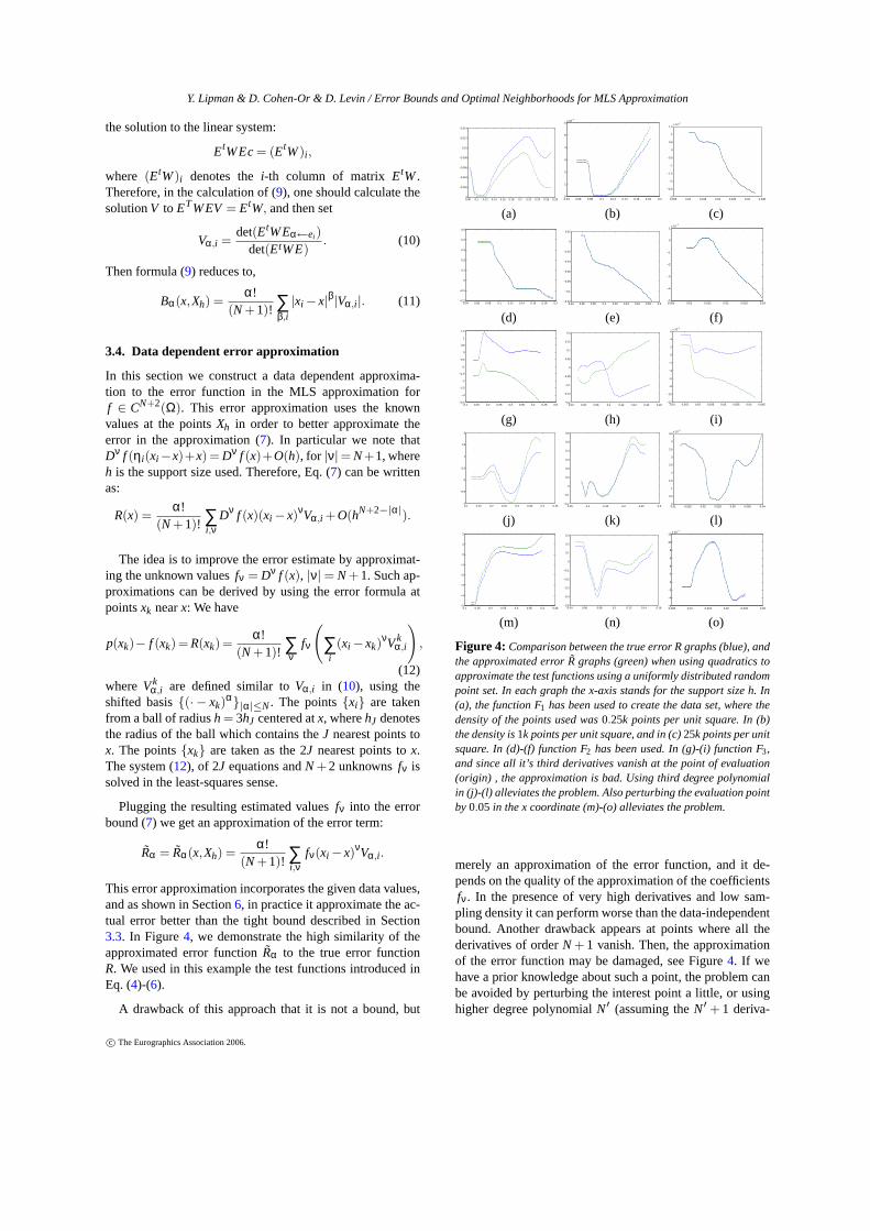
This error approximation incorporates the given data values,and as shown in Section6, in practice it approximate the ac-tual error better than the tight bound described in Section3.3. In Figure4, we demonstrate the high similarity of theapproximated error functionRα to the true error functionR. We used in this example the test functions introduced inEq. (4)-(6).

A drawback of this approach that it is not a bound, but

0.08 0.1 0.12 0.14 0.16 0.18 0.2 0.22 0.24 0.26 0.280

0.002

0.004

0.006

0.008

0.01

0.012

0.014

0.04 0.06 0.08 0.1 0.12 0.14 0.16 0.18 0.20

1

2

3

4

5

6x 10−3

0.005 0.01 0.015 0.02 0.025 0.03 0.035−3

−2.5

−2

−1.5

−1

−0.5

0

0.5

1

1.5x 10−3

(a) (b) (c)

0.04 0.06 0.08 0.1 0.12 0.14 0.16 0.18 0.2−0.2

−0.1

0

0.1

0.2

0.3

0.4

0.5

0.04 0.06 0.08 0.1 0.12 0.14 0.16 0.18 0.2−0.12

−0.1

−0.08

−0.06

−0.04

−0.02

0

0.02

0.005 0.01 0.015 0.02 0.025 0.03−5

−4

−3

−2

−1

0

1x 10−3

(d) (e) (f)

0.1 0.15 0.2 0.25 0.3 0.35 0.4 0.45 0.5−3.5

−3

−2.5

−2

−1.5

−1

−0.5

0

0.5

1

1.5

0.04 0.06 0.08 0.1 0.12 0.14 0.16 0.18−0.2

−0.15

−0.1

−0.05

0

0.05

0.1

0.15

0.2

0.01 0.015 0.02 0.025 0.03 0.035 0.04 0.045−12

−10

−8

−6

−4

−2

0

2

4

6x 10−3

(g) (h) (i)

0.1 0.15 0.2 0.25 0.3 0.35 0.4 0.45−1

−0.5

0

0.5

1

1.5

2

0.05 0.1 0.15 0.2 0.25 0.3−0.2

−0.1

0

0.1

0.2

0.3

0.4

0.5

0.6

0.01 0.015 0.02 0.025 0.03 0.035 0.040

0.5

1

1.5

2

2.5

3

3.5

4

4.5x 10−3

(j) (k) (l)

0.1 0.15 0.2 0.25 0.3 0.35 0.4 0.45−5

−4

−3

−2

−1

0

1

2

0.04 0.06 0.08 0.1 0.12 0.14 0.16−0.5

−0.4

−0.3

−0.2

−0.1

0

0.1

0.2

0.3

0.005 0.01 0.015 0.02 0.025 0.03−6

−4

−2

0

2

4

6

8

10

12x 10−3

(m) (n) (o)

Figure 4: Comparison between the true error R graphs (blue), andthe approximated errorR graphs (green) when using quadratics toapproximate the test functions using a uniformly distributed randompoint set. In each graph the x-axis stands for the support size h. In(a), the function F1 has been used to create the data set, where thedensity of the points used was0.25k points per unit square. In (b)the density is1k points per unit square, and in (c)25k points per unitsquare. In (d)-(f) function F2 has been used. In (g)-(i) function F3,and since all it’s third derivatives vanish at the point of evaluation(origin) , the approximation is bad. Using third degree polynomialin (j)-(l) alleviates the problem. Also perturbing the evaluation pointby0.05 in the x coordinate (m)-(o) alleviates the problem.

merely an approximation of the error function, and it de-pends on the quality of the approximation of the coefficientsfν. In the presence of very high derivatives and low sam-pling density it can perform worse than the data-independentbound. Another drawback appears at points where all thederivatives of orderN + 1 vanish. Then, the approximationof the error function may be damaged, see Figure4. If wehave a prior knowledge about such a point, the problem canbe avoided by perturbing the interest point a little, or usinghigher degree polynomialN′ (assuming theN′ + 1 deriva-

c© The Eurographics Association 2006.

Y. Lipman & D. Cohen-Or & D. Levin / Error Bounds and Optimal Neighborhoods for MLS Approximation

tives do not all vanish at that point), in Figure4, where all thethird derivatives ofF3 vanish at the origin (the point of inter-est in that example) the approximation of the error functionis quite inaccurate, however using third degree polynomialor moving the point of interest a little alleviates the problem.The reason of this phenomenon lies in the fact that the signof the coefficientsDν f (ηi(xi−x)+x) are likely to change inthe vicinity ofx, hence the error function is highly dependenton the values ofηi .

3.5. Noisy Data

In this section we extend our previous error bounds and ap-proximations to optimally handle errors (noise) in the sam-pled data. We assume that errorsεi , where|εi | ≤ ε are in-troduced into the data, that is,f ∗(xi) = f (xi)+ εi , where fstands for the ’true’ sampled function.

It then follows,as in Theorem3.1, that

R∗(x) = R(x)+α!I

∑i=1

εiVα,i ,

where R∗(x) = Dα p(x)− Dα f ∗(x) and R(x) is given inEq. (7). Hence,

|R∗(x)| ≤ |R(x)|+α!εI

∑i=1

|Vα,i |. (13)

Note that this bound is again tight since no assumption canbe made on the signs ofεi nor their magnitude, except that|εi | ≤ ε.

In Figure2, using the points inside the black circle (b),which are chosen by the heuristic method, in the MLS ap-proximation leads to∑I

i=1 |Vα,i | ≈ 15 forα = (0,0) and≈ 99for α = (1,0). Hence, we can suspect that the noise level inthe data might be amplified by these factors when approxi-mating the value or the partial derivative∂x at the red point,respectively. Indeed, thetrue error in the function evalua-tion is∼ 9ε and the error in the derivative approximation is∼ 106ε. Minimizing the bound (13) imply choosing a big-ger support size in this case, which results in∼ 0.17ε and∼ 3.3ε error in approximation of the value and derivativesrespectively. In section3.6we discuss another aspect of theerror amplification phenomenon.

Next, we integrate the sampling error term into the formererror terms. First the data dependent approximation,

|R∗(x)| |R(x)|+α!εI

∑i=1

|Vα,i |,

where stands for≤ up to a term of magnitudeO(h).Therefore, we denote our approximated error in the approx-imation:

Rα,ε(x,Xh) = |Rα(x,Xh)|+α!εI

∑i=1

|Vα,i |. (14)

For the data-independent bound:

|R∗(x)| ≤C|Bα(x,Xh)|+α!εI

∑i=1

|Vα,i |.

SinceC is unknown, this bound is better presented if we con-sider relative error, i.e.,f (xi) = f ∗(xi)(1+ εi). In this caseby similar consideration as before, the tight error bound inthe presence of noise in the data becomes:

|R∗(x)| ≤C

(|Bα(x,Xh)|+α!ε

I

∑i=1

|Vα,i |

), (15)

whereC bounds the relevant derivatives and the function val-ues. In practice we considered the term in the parentheses asthe function to be minimized in the presence of noise in thedata:

Bα,ε(x,Xh) = |Bα(x,Xh)|+α!εI

∑i=1

|Vα,i |. (16)

3.6. A Confidence Measure

By Corollary3.1and Eq. (15) we have that

|Dα p(x)−Dα f (x)| ≤CBα,ε(x,Xh),

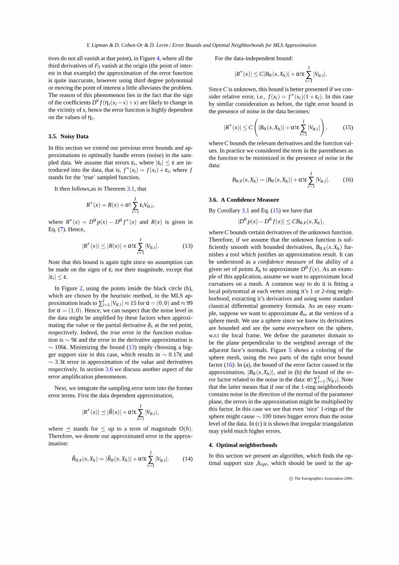
whereC bounds certain derivatives of the unknown function.Therefore, if we assume that the unknown function is suf-ficiently smooth with bounded derivatives,Bα,ε(x,Xh) fur-nishes a tool which justifies an approximation result. It canbe understood as aconfidence measureof the ability of agiven set of pointsXh to approximateDα f (x). As an exam-ple of this application, assume we want to approximate localcurvatures on a mesh. A common way to do it is fitting alocal polynomial at each vertex using it’s 1 or 2-ring neigh-borhood, extracting it’s derivatives and using some standardclassical differential geometry formula. As an easy exam-ple, suppose we want to approximate∂xx at the vertices of asphere mesh. We use a sphere since we know its derivativesare bounded and are the same everywhere on the sphere,w.r.t the local frame. We define the parameter domain tobe the plane perpendicular to the weighted average of theadjacent face’s normals. Figure5 shows a coloring of thesphere mesh, using the two parts of the tight error boundfactor (16): In (a), the bound of the error factor caused in theapproximation,|Bα(x,Xh)|, and in (b) the bound of the er-ror factor related to the noise in the data:α! ∑I

i=1 |Vα,i |. Notethat the latter means that if one of the 1-ring neighborhoodscontains noise in the direction of the normal of the parameterplane, the errors in the approximation might be multiplied bythis factor. In this case we see that even ’nice’ 1-rings of thesphere might cause∼ 100 times bigger errors than the noiselevel of the data. In (c) it is shown that irregular triangulationmay yield much higher errors.

4. Optimal neighborhoods

In this section we present an algorithm, which finds the op-timal support size ,hopt, which should be used in the ap-

c© The Eurographics Association 2006.

Y. Lipman & D. Cohen-Or & D. Levin / Error Bounds and Optimal Neighborhoods for MLS Approximation

0.007

0.073

0.139

52.7

78.2

103.8

32

752

1472

(a) (b) (c)

Figure 5: Color maps of the confidence measures for approximat-ing ∂xx using quadratic polynomial fitted in the least-squares senseto the 1-ring neighborhoods on a sphere mesh. In (a) the (tight)error bound factor Bα caused in the approximation, for non-noisydata. In (b) the factors which multiply the noiseε in the data. Notethat small noise level in the data may still cause∼ 100times biggererrors in the approximation. (c) is the same as (b) for an irregularsphere mesh.

proximation procedure (1)-(2) to ensure minimal error. Webase our algorithm on the error analysis presented in for-mer sections, i.e., equations (14) and (16). More specifically,for a givenX,α,N and a point where the approximation issought,x, we look for the optimalh, which we denote byhopt, which minimizes the bound or the approximation ofthe error|Dα f (x)−Dα p(x)|.

4.1. Finding an Optimal Support Size

We use the same algorithm for both bounds (14) and (16).We look for the support sizeh which minimizes the boundfunction EBα(x,X,h), where for brevity we will use thesymbolEBα for both bounds.

We fix an upper and lower boundsHmin,Hmax for h,e.g., Hmin could be set tohJ (which is defined in Sec-tion 3.4) and Hmax to some large support size radius, weused for example 4hJ. A rough step size∆ is set, e.g.,we used|Hmax−Hmin|/50, and the algorithm traverseh =Hmin,Hmin+ ∆, ...,Hmax where for eachh the algorithm cal-culates the error bound functionEBα, for the data pointsXh. Next, after extracting the minimizing support size ra-

diush(0)opt = argminh=Hmin+ j∆EBα(x,X,h), we further im-

prove the approximation tohopt by fitting an interpolating

quadratic nearh(0)opt and minimize it to defineh(1)

opt. We iterate

this procedure until|h(k+1)opt −h(k)

opt| ≤ tolerance. In our appli-

cation we actually minimizedEB2, for faster convergence.

For efficient computation the following considerations areemployed. First we move the origin tox, i.e., we use thepointsxi := xi −x ,i = 1, .., I . Second, we rearrangexi ∈ X∩BHmax(0) with respect to their distance from 0 (x), where nowthe sub-indexi is with respect to this ordering. IfE is theVandermonde matrix based on the data pointsx1, ...,xI , thenthe matrixE′ for the data pointsx1, ...,xI+1 can be writtenasE′i, j = Ei, j for i ≤ I andEI+1, j = p j (xI+1). This impliesthat whenh changes to include a new pointxI+1 in Xh, weonly need to add a single row to the previous VandermondematrixE, to construct the Vandermonde matrix forXh.

Note that if we have calculated the bound for the datapoints x1, ...,xI , then the quantity∑|β|=N+1 |xi |β for i =1, .., I should be re-used and the only new calculation thatshould be performed is∑|β|=N+1 |xI+1|β. Taking into con-sideration all the above remarks, whenh is changed to in-clude a new point, the most time consuming part of the cal-culation consists of factorization ofJ× J matrix (for exam-ple for quadratic interpolation we haveJ = 6), and back-substitution forI vectors (the matrixEtW), this leads to anO(J3 +J2I) complexity for each step of the algorithm. Thisis multiplied by the number of iterations of the algorithm,which in our implementation is≤ 100. In the case of usingthe data dependent bound, there is a preprocess step of solv-ing for the coefficientsfν as explained in Section3.4. Thecomputational cost of this step isO(J4 +J3I).

An important consequence of the above procedure is thatsinceV is calculated anyway, we actually get for no sig-nificant extra calculations the bound of the error for anyα,|α| ≤ N, that is, the bound for every possible derivative (andvalue) approximation.

It should be noted that to get consistenth values,we take the first global minimum (if there is more thanone zero). Another delicate point, is that the parametervaluehmin of the minimum ofEBα(x,X,h), i.e., hmin(x) =argminhEBα(x,X,h), is a piecewise smooth function ofx if the neighborhoods used in the approximation offν aresmoothly chosen. This implies that the MLS approximation,based on thish field, is only piecewise smooth.

4.1.1. Integrating with the MLS projection operator

All the previous construction dealt with a function over a pa-rameter space. When dealing with a point cloud there is nonatural choice of such space. A popular method for choos-ing this space in the case of surfaces is the MLS projectionoperator [Lev03,ABCO∗01,PKKG03,AK04]. After choos-ing the parameter space, in this case a plane, we are back toour original functional settings, with a minor difference: thedistance to the neighboring points is measured using theiractual position in space and not their projection on the pa-rameter space, i.e.,p is defined by minimizing

I

∑i=1

( f (xi)− p(xi))2 ηh(‖(xi , f (xi))− (x,z)‖),

where(x,z) is chosen by the first step of the MLS projection.This small change can be easily incorporated in our system,one just have to redefine the way distances are measured. Wehave integrated that into our system and noticed two interest-ing results: For the test functionF1,F2 the results were sim-ilar to the algorithm which measured the distance on the pa-rameter space (results are demonstrated in Section6). How-ever, In the case of data taken fromF3, since the function israpidly oscillating, the new distance measure is likely to pre-fer points from other periods and not from close parametervalues, and the approximation quality deteriorates.

c© The Eurographics Association 2006.

Y. Lipman & D. Cohen-Or & D. Levin / Error Bounds and Optimal Neighborhoods for MLS Approximation

density Lx f N ε H σ(H).25k f (x) F1 2 0 2.24 0.74.25k f (x) F2 2 0 2.15 0.731k f (x) F2 2 0 2.1 0.691k f (x) F1 2 0 2.3 0.751k f (x) F1 3 0 1.88 0.571k ∂x f (x) F1 3 0 2.28 0.744k ∂xy f (x) F2 3 0 2.06 0.74.5k f (x) F3 2 10−2 2.41 0.77.5k f (x) F3 2 10−4 2.35 0.77.5k ∂x f (x) F2 2 10−5 2.25 0.8

Table 1: Experiments results used to derive the heuristic supportsize rule.

5. Heuristics

In this section we present the derivation of the heuristicmethod for choosing a support sizeh, which we later usefor comparison with the optimal choice. The method is de-rived by experiments, in the following way: We consider thetrueerror of our MLS approximation procedure as a functionof the support size usedh. We leth vary from it’s minimalvalue, i.e., the radiushJ of the ball containing theJ nearestneighbors up to 4 times this radius. It is observed that theminimum can be predicted as a certain constant timeshJ.The heuristic is based on finding the right constant, and wedo it by extensive simulation. We define the random variable

H =hbest

hJ,

wherehbest stands for the true optimal support size, i.e., thesupport size which minimizes the true error function in theinterval [hJ,4×hJ]. In table1, we specify several measure-ments ofH, in particular we consider different test functions(4)-(6), point densities, noisy and non-noisy data, quadraticand cubic polynomial and different functionals. The den-sity specify the number of data points per unit square.Hwas sampled in a grid inside the domain[−1,1]× [−1,1].The meanH and standard deviationσ(H) are computed. Ingeneral the results of the different scenarios are similar: theH is approximately 2.2 andσ(H) is generally around 0.75.Therefore, our heuristic choice of support size to be used inthe MLS approximation ish = 2.2hJ.

A similar heuristic for choosing the support sizeh maybe obtained by using the error boundBα, as follows: For agiven distribution of data points near the origin we find theoptimalh minimizing Bα, and computehopt/hJ. Averagingthese ratios over many randomly chosen distributions of datapoints, we obtain for example, an average ratio∼ 1.9 forquadratic polynomial approximation of the function value,N = 2, α = (0,0), and ratio∼ 2.4 for N = 2, α(1,0) withnoise level of 10−5. Another option is to compute a differentrule for each noise levelε, but we didn’t pursue this direc-tion.

−0.5 −0.4 −0.3 −0.2 −0.1 0 0.1 0.2 0.3 0.4 0.5−0.5

−0.4

−0.3

−0.2

−0.1

0

0.1

0.2

0.3

0.4

0.5

(a)

−0.2−0.1

00.1

0.20.3

−0.2−0.1

00.1

0.20.3

0

1

2

3

4

5

6

x 10−3

−0.2−0.1

00.1

0.20.3

−0.2−0.1

00.1

0.20.3

0

1

2

3

4

5

6

x 10−3

error optimal esen

(b) (c)

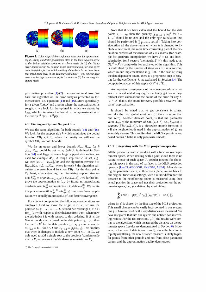
Figure 6: An example of data set with irregular density. We usedquadratic polynomials in the MLS approximation, and resampled inthe drawn rectangle (a). In (b) the error resulted using the heuristicsupport size h. In (c) the optimal h has been used. The error ratioE1 is 0.37.

−1 −0.8 −0.6 −0.4 −0.2 0 0.2 0.4 0.6 0.8 1−1

−0.8

−0.6

−0.4

−0.2

0

0.2

0.4

0.6

0.8

1

−1

−0.5

0

0.5

1

−1

−0.5

0

0.5

1

0

1

2

3

x 10−3

error naive

−1

−0.5

0

0.5

1

−1

−0.5

0

0.5

1

0

1

2

3

x 10−3

error optimal esen

(a) (b) (c)

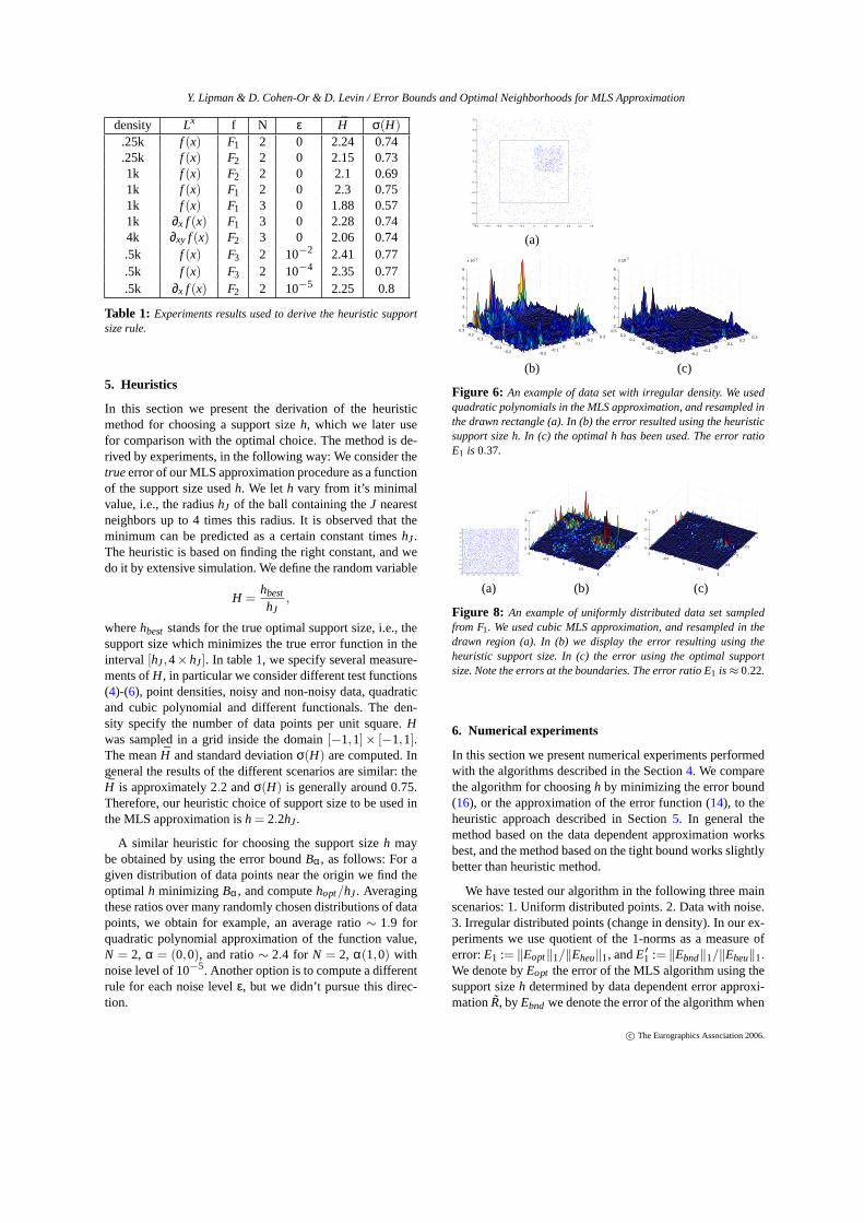
Figure 8: An example of uniformly distributed data set sampledfrom F1. We used cubic MLS approximation, and resampled in thedrawn region (a). In (b) we display the error resulting using theheuristic support size. In (c) the error using the optimal supportsize. Note the errors at the boundaries. The error ratio E1 is≈ 0.22.

6. Numerical experiments

In this section we present numerical experiments performedwith the algorithms described in the Section4. We comparethe algorithm for choosingh by minimizing the error bound(16), or the approximation of the error function (14), to theheuristic approach described in Section5. In general themethod based on the data dependent approximation worksbest, and the method based on the tight bound works slightlybetter than heuristic method.

We have tested our algorithm in the following three mainscenarios: 1. Uniform distributed points. 2. Data with noise.3. Irregular distributed points (change in density). In our ex-periments we use quotient of the 1-norms as a measure oferror:E1 := ‖Eopt‖1/‖Eheu‖1, andE′1 := ‖Ebnd‖1/‖Eheu‖1.We denote byEopt the error of the MLS algorithm using thesupport sizeh determined by data dependent error approxi-mationR, byEbnd we denote the error of the algorithm when

c© The Eurographics Association 2006.

Y. Lipman & D. Cohen-Or & D. Levin / Error Bounds and Optimal Neighborhoods for MLS Approximation

−1 −0.8 −0.6 −0.4 −0.2 0 0.2 0.4 0.6 0.8 1−1

−0.8

−0.6

−0.4

−0.2

0

0.2

0.4

0.6

0.8

1

(a) (b) (c) (d) (e)

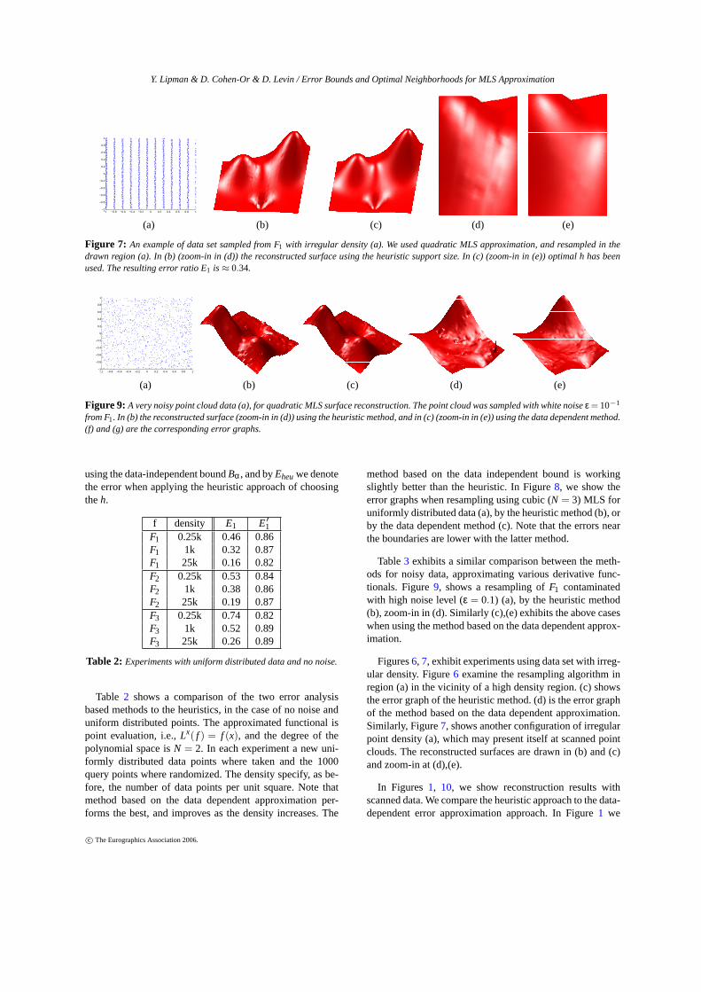
Figure 7: An example of data set sampled from F1 with irregular density (a). We used quadratic MLS approximation, and resampled in thedrawn region (a). In (b) (zoom-in in (d)) the reconstructed surface using the heuristic support size. In (c) (zoom-in in (e)) optimal h has beenused. The resulting error ratio E1 is≈ 0.34.

−1 −0.8 −0.6 −0.4 −0.2 0 0.2 0.4 0.6 0.8 1−1

−0.8

−0.6

−0.4

−0.2

0

0.2

0.4

0.6

0.8

1

(a) (b) (c) (d) (e)

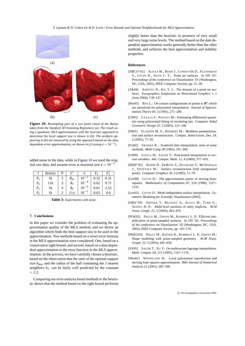
Figure 9: A very noisy point cloud data (a), for quadratic MLS surface reconstruction. The point cloud was sampled with white noiseε = 10−1

from F1. In (b) the reconstructed surface (zoom-in in (d)) using the heuristic method, and in (c) (zoom-in in (e)) using the data dependent method.(f) and (g) are the corresponding error graphs.

using the data-independent boundBα, and byEheuwe denotethe error when applying the heuristic approach of choosingtheh.

f density E1 E′1F1 0.25k 0.46 0.86F1 1k 0.32 0.87F1 25k 0.16 0.82F2 0.25k 0.53 0.84F2 1k 0.38 0.86F2 25k 0.19 0.87F3 0.25k 0.74 0.82F3 1k 0.52 0.89F3 25k 0.26 0.89

Table 2: Experiments with uniform distributed data and no noise.

Table 2 shows a comparison of the two error analysisbased methods to the heuristics, in the case of no noise anduniform distributed points. The approximated functional ispoint evaluation, i.e.,Lx( f ) = f (x), and the degree of thepolynomial space isN = 2. In each experiment a new uni-formly distributed data points where taken and the 1000query points where randomized. The density specify, as be-fore, the number of data points per unit square. Note thatmethod based on the data dependent approximation per-forms the best, and improves as the density increases. The

method based on the data independent bound is workingslightly better than the heuristic. In Figure8, we show theerror graphs when resampling using cubic (N = 3) MLS foruniformly distributed data (a), by the heuristic method (b), orby the data dependent method (c). Note that the errors nearthe boundaries are lower with the latter method.

Table3 exhibits a similar comparison between the meth-ods for noisy data, approximating various derivative func-tionals. Figure9, shows a resampling ofF1 contaminatedwith high noise level (ε = 0.1) (a), by the heuristic method(b), zoom-in in (d). Similarly (c),(e) exhibits the above caseswhen using the method based on the data dependent approx-imation.

Figures6, 7, exhibit experiments using data set with irreg-ular density. Figure6 examine the resampling algorithm inregion (a) in the vicinity of a high density region. (c) showsthe error graph of the heuristic method. (d) is the error graphof the method based on the data dependent approximation.Similarly, Figure7, shows another configuration of irregularpoint density (a), which may present itself at scanned pointclouds. The reconstructed surfaces are drawn in (b) and (c)and zoom-in at (d),(e).

In Figures1, 10, we show reconstruction results withscanned data. We compare the heuristic approach to the data-dependent error approximation approach. In Figure1 we

c© The Eurographics Association 2006.

Y. Lipman & D. Cohen-Or & D. Levin / Error Bounds and Optimal Neighborhoods for MLS Approximation

(a)

(b) (c)

Figure 10: Resampling part of a raw point cloud of the Bunnytaken from the Stanford 3D Scanning Repository (a). The result us-ing a quadratic MLS approximation with the heuristic approach todetermine the local support size is shown in (b). The artifacts ap-pearing in (b) are removed by using the approach based on the datadependent error approximation, as shown in (c) (usingε = 10−5).

added noise to the data, while in Figure10we used the orig-inal raw data, and assume error at maximal sizeε = 10−5.

f density N Lx ε E1 E′1F1 1k 3 ∂xy 10−2 0.32 0.31F2 11k 3 ∂x 10−4 0.62 0.71F1 1k 3 ∂y 10−5 0.61 2.53F2 1k 2 f (x) 10−1 0.63 0.6

Table 3: Experiments with noise.

7. Conclusions

In this paper we consider the problem of evaluating the ap-proximation quality of the MLS method, and we derive analgorithm which finds the best support size to be used in theapproximation. Two methods based on a novel error formulain the MLS approximation were considered: One, based on aconservative tight bound, and second, based on a data depen-dent approximation to the error function in the MLS approx-imation. In the process, we have carefully chosen a heuristic,based on the observation that the ratio of the optimal supportsizehbest and the radius of the ball containing theJ nearestneighborshJ, can be fairly well predicted by the constant∼ 2.2.

Comparing our error analysis based methods to the heuris-tic shows that the method based on the tight bound performs

slightly better than the heuristic in presence of very smalland very large noise levels. The method based on the data de-pendent approximation works generally better than the othermethods, and achieves the best approximation and stabilityproperties.

References

[ABCO∗01] ALEXA M., BEHR J., COHEN-OR D., FLEISHMAN

S., LEVIN D., SILVA C. T.: Point set surfaces. InVIS ’01:Proceedings of the conference on Visualization ’01(Washington,DC, USA, 2001), IEEE Computer Society, pp. 21–28.

[AK04] AMENTA N., KIL Y. J.: The domain of a point set sur-faces. Eurographics Symposium on Point-based Graphics 1, 1(June 2004), 139–147.

[Bos91] BOS L.: On certain configurations of points inIRn whichare unisolvent for polynomial interpolation.Journal of Approxi-mation Theory 64, 3 (1991), 271–280.

[CP05] CAZALS F., POUGET M.: Estimating differential quanti-ties using polynomial fitting of osculating jets.Computer AidedGeometric Design 22, 2 (2005), 121–146.

[FR01] FLOATER M. S., REIMERS M.: Meshless parameteriza-tion and surface reconstruction.Comput. Aided Geom. Des. 18,2 (2001), 77–92.

[Fra82] FRANKE R.: Scattered data interpolation: tests of somemethods.Math Comp 38(1982), 181–200.

[GS00] GASCA M., SAUER T.: Polynomial interpolation in sev-eral variables.Adv. Comput. Math. 12, 4 (2000), 377–410.

[HDD∗92] HOPPEH., DEROSET., DUCHAMP T., MCDONALD

J., STUETZLE W.: Surface reconstruction from unorganizedpoints.Computer Graphics 26, 2 (1992), 71–78.

[Lev98] LEVIN D.: The approximation power of moving least-squares. Mathematics of Computation 67, 224 (1998), 1517–1531.

[Lev03] LEVIN D.: Mesh-independent surface interpolation.Ge-ometric Modeling for Scientific Visualization(2003).

[OBA∗03] OHTAKE Y., BELYAEV A., ALEXA M., TURK G.,SEIDEL H.-P.: Multi-level partition of unity implicits. ACMTrans. Graph. 22, 3 (2003), 463–470.

[PGK02] PAULY M., GROSSM., KOBBELT L. P.: Efficient sim-plification of point-sampled surfaces. InVIS ’02: Proceedingsof the conference on Visualization ’02(Washington, DC, USA,2002), IEEE Computer Society, pp. 163–170.

[PKKG03] PAULY M., KEISERR., KOBBELT L. P., GROSSM.:Shape modeling with point-sampled geometry.ACM Trans.Graph. 22, 3 (2003), 641–650.

[SX95] SAUER T., XU Y.: On multivariate lagrange interpolation.Math. Comput. 64, 211 (1995), 1147–1170.

[Wen01] WENDLAND H.: Local polynomial reproduction andmoving least squares approximation.IMA Journal of NumericalAnalysis 21(2001), 285–300.

c© The Eurographics Association 2006.