Error of the network approximation for densely packed ...

Error of the network approximation for denselypacked composites with irregular geometry

Leonid Berlyand�

Alexei Novikov�

August 12, 2001

Contents

1 Introduction. Overview of the paper 2

2 Formulation 72.1 The mathematical model . . . . . . . . . . . . . . . . . . . . . . . . 72.2 Direct and dual variational formulations . . . . . . . . . . . . . . . . 9

3 Construction of the discrete network 103.1 Effective conductivity for periodic square and hexagonal lattices . . . 103.2 The discrete network for densely packed high contrast composites . . 153.3 The triangle-neck partition . . . . . . . . . . . . . . . . . . . . . . . 203.4 The discrete minimization problem . . . . . . . . . . . . . . . . . . . 24

4 Variational bounds on the effective conductivity 294.1 The lower bound . . . . . . . . . . . . . . . . . . . . . . . . . . . . 304.2 The upper bound . . . . . . . . . . . . . . . . . . . . . . . . . . . . 324.3 The error estimate . . . . . . . . . . . . . . . . . . . . . . . . . . . . 344.4 A numerical illustration . . . . . . . . . . . . . . . . . . . . . . . . . 42

5 Conclusions 45

A Appendix. Auxiliary estimates 46A.1 Estimates on the relative neck widths . . . . . . . . . . . . . . . . . . 46A.2 Gradient estimates inside the necks . . . . . . . . . . . . . . . . . . . 49A.3 Comparison of fluxes for the two discrete networks . . . . . . . . . . 51A.4 Gradient estimates inside the triangles . . . . . . . . . . . . . . . . . 53

�Department of Mathematics, 414 McAllister Building, Pennsylvania State University, University Park,

PA 16802, USA ([email protected])�IMA, University of Minnesota, 400 Lind Hall, 207 Church S.E., Minneapolis, MN 55455, USA. Present

address: California Institute of Technology, Applied & Computational Mathematics, 1200 E. CaliforniaBoulevard, MC 217-50, Pasadena, CA 91125, USA ([email protected])

1

Abstract

We apply a discrete network approximation to the problem of the effective con-ductivity of the high contrast, highly packed composites. The inclusions are irreg-ularly (randomly) distributed in the hosting medium, so that a significant fractionof them may not participate in the conducting spanning cluster. For this class ofinclusion distributions we derive a discrete network approximation and obtain an apriori error estimate for this approximation in which all the constants are explicitlycomputed. Explicit dependence on the irregular geometry of the inclusions’ arrayis obtained.

We use variational techniques to provide rigorous mathematical justificationfor the approximation and its error estimate.

Key words. effective conductivity, discrete network, error estimate, variational bounds

AMS subject classifications. 74Q05, 35Q72, 94C05

1 Introduction. Overview of the paper

We study the effective properties such as the effective conductivity or the effectivedielectric constant of composite materials in which a large number of inclusions (filler)are irregularly (randomly) distributed in a homogeneous hosting medium (matrix). Forease of presentation and clarity we concentrate here on the effective conductivity. Weare particularly interested in the case of the high contrast, highly packed particularcomposites, that is when the conductivity of the inclusions is much larger than theconductivity of the hosting medium and the volume fraction of the inclusions is veryhigh. High contrast composites are extremely attractive for the design of new materialswith physical properties better than those of their constituents. The case when theconcentration of the filling inclusions is high is particularly relevant to polymer/ceramiccomposites, because a polymer matrix compensates for the brittle nature of ceramicswhich is their main weakness. A survey on the relevant engineering problems in twoand three dimensions (fibers and particles in a matrix) can be found in [4].

Our main tool is the discrete network approximation of [4] for a two dimensionalcomposite, where the inclusions are modeled as identical disks. We focus on the twokey issues arising for this approximation. The first is the explicit error estimate ofthe discrete network approximation to the continuum problem of effective conductiv-ity. The second is a quantitative estimate on how the connectivity patterns for variousirregular distributions of the inclusions affect the effective conductivity.

The main advantage of our discrete network approximation is that it is easy to im-plement numerically and at the same time it captures geometric patterns of the locationof inclusions in the matrix. The importance of the geometric patterns in evaluation ofthe effective properties of high contrast composites can be seen in the analysis of peri-odic structures. It was observed that for such periodic composites of moderate volumefraction, that is away from the almost touching situation, the effective conductivity is oforder of the conductivity of the matrix (see, for example, [2], [17], [18], and referencestherein). In other words, the filler has almost no effect on the effective conductivity.However, in the case of almost touching inclusions, the effective conductivities of two

2

ERROR OF DISCRETE NETWORK 3

periodic structures with different locations of inclusions in the matrix can be signifi-cantly different for the same volume fraction. For example, if the contrast ratio of theconstituents is assumed to be � , then for the same volume fraction of disks (equal to�� ) for the hexagonal lattice, the effective conductivity � �� (see theorem 3.1 inthis paper), while for the square lattice � �� (see [14]).

The case of irregularly distributed inclusions is less well-understood. Since thevolume fraction of the inclusions is high, the irregular connectivity patterns in thewhole composite (percolation effects) determine the behavior of the effective prop-erties. Moreover, it was observed that the irregular connectivity patterns of conductinginclusions can greatly increase the effective conductivity. Therefore, there is a needfor a simple model that is still able to capture percolation effects. Also, while for agiven periodic structure the volume fraction of the inclusions uniquely determines thedistances between the inclusions, this is no longer true for irregular structures and oneshould search for a model with a new parameter, which describes the local geometrywhen the inclusions are close to touching. Such a model (the network approximation)was proposed in [4] in two dimensions. Based on the Voronoi tessellation the notionof the interparticle distance parameter for closely packed (“randomized” hexagonal)patterns was introduced there. In the present work we generalize this notion for abroad class of geometrical patterns. This is important, because in spite of the fact thatthe hexagonal lattice is the densest packing in two dimensions, it is hard at present tomanufacture particulate composites with this packing of inclusions. Our new approachallows to derive an explicit error estimate for the network approximation. Such es-timates are rare in homogenization theory, most of the existing estimates provide anorder of the magnitude of the error only. The class of geometrical patterns that canbe handled by our approach includes the situation of a nonuniform irregular distribu-tion, when a significant fraction of the inclusions does not participate in the conductingspanning cluster. This approach allows to relax the close packing condition of [4], sothat not all the “neighboring” disks are closely spaced. More specifically we intro-duce and study the �� close packing condition, which loosely speaking allows for“holes” with the perimeter of order �� in the conducting spanning cluster. Here �is the radius of the particles, and � is the “size of holes in the conducting clusters”(see figure 1.1). Thus we account quantitatively for the presence of these holes in thecomposite.

The question of error estimates was raised by I. Babuska, because the analysis of[4] is asymptotic in the interparticle distance parameter and does not provide an errorestimate. The analysis in the present paper does not use asymptotics and it holds forany (small) finite value of the relative interparticle distance parameter. This enables usto prove the following error estimate for the effective conductivity � � .

� � ��

� � �!��" ��$# (1.1)

where � is the value of effective conductivity provided by the network approximation,� � � is the relative interparticle distance. We evaluate the constant� �%�&� explicitly.

For small perturbations of the hexagonal lattice �'�)( , � �*(%�+�-,/. 01, ; for a less dense“almost square” packing �2� � , � � � �3�4(156.87 � ; for an arbitrary � we provide an

4 L. BERLYAND AND A. NOVIKOV

��

��

��

��

��

��

��

��

��

��

��

��

� � � � � � � � � � � � � � � � � � � � � � � �

��

��

��

"hole"

"hole"

"hole""hole"

"hole"

(a) Black disks form the conducting cluster.Hatched disks do not participate in the cluster.

8−gon

9−gon

5−gon

10−gon

11−gon

15−gon

3−gon

(b) The graph that corresponds to the conducting cluster in (a). An � -gon � � �corresponds to a “hole” of size � .

Figure 1.1: The conducting cluster in a composite with “holes”.


upper bound� �%�&� ��6. ,15 �� .

The discrete network models for various high contrast composites have been usedextensively in the physics literature (see [1], [11], [13], [15], [20], [21]); however, therelation between the network and the underlying continuum problem was not studiedthere. In [16], high contrast conductivity problems were first formulated and analyzedusing variational methods. There the high contrast field was of the form�� (1.2)

with a smooth function � �� . In particular, the asymptotic analysis in the high contrastratio parameter � has been carried out in [16] for a random checkerboard model.

For the Kozlov’s function (1.2) a network asymptotic approximation in the highcontrast parameter � was developed in [6], [7], [8], [9]. It was rigorously proved in[8] that the network approximates the original continuum problem. The analysis of[8] was carried out for high contrast continuum problems arising in imaging, when thematerials’ properties are not known and it is convenient to model the high contrast ina simple geometric manner by using (1.2). In this model the key parameter, whichdetermines the conductivity of the edges in the network, is � �� , where �� and�� are the principal curvatures at the saddle points of � �� .

Our analysis applies to a class of physical problems where � �� is not smooth. Inour case � �� is the characteristic function of the disks

� �� $� � � if �� "!$#%if �'&)(3�+*-�,�"! # #

here ! # , - � � # . . . #/. are non-overlapping disks, * �10 �32 # 2547680 % # �94 is a a two-dimensional rectangular domain, &$( �8* �:�"! # is the hosting matrix (see figure 2.1).

Furthermore, in our case the high contrast parameter � � % . In other words, we con-sider the infinite contrast material with ideally conducting inclusions. This assumptionis valid for a variety of particulate composites (particles or fibers in a matrix) and it is inagreement with bounds [10] which imply that if the contrast ratio is greater than severalhundreds, then for practical purposes it can be taken to be infinite. More precisely, ifone plots the effective conductivity versus the contrast ratio using formulas from [10],then the curve becomes almost horizontal after the contrast ratio reaches values about� %�; .

Our construction of the discrete network approximation for the problem of the ef-fective conductivity is as follows. Suppose the potential < ��>= # �@? � is a piece-wise dif-ferentiable function on * , which is constant on each disk !A# , and takes values � � and� on the lower and the upper boundaries respectively, that is< �� = # � ? � �+B # # if �� = # � ? �C�D! # # < �� = # � �� # <�� = # � � � �1. (1.3)

The goal here is to find the effective conductivity

� �� 2AE$FHGIKJ�LNM � O < � ?QP x # (1.4)

where minimum is taken over an appropriate class of admissible functions.


The discrete network model is based on the observation that the fluxesO < are

significant only in certain areas (“necks”) between closely spaced disks, and in thesenecks the fluxes can be easily computed. For two disks ! # and ! � the computation ofthe flux in the neck * # � between them relies on the observation due to J.B. Keller in[14] that as the distance between the disks � # �� %

, the potential < in the neck can beapproximated by a linear interpolation between the potentials B # and B � on disks ! # and! � respectively.

The discrete network model is a graph where the vertices are the centers of thedisks ! # and the edges correspond to the necks * # � between neighbors with length � # � .Neighbors are defined as disks that share a common edge of the Voronoi tessellationof the rectangular domain * with respect to the centers of the disks. To each edge anumber (specific flux) � # � is assigned, computed by solving the two-disk problem withfixed potentials < � ! # �� and < � ! � � � % in infinite space. The value of effectiveconductivity, provided by this model is the energy of the discrete network:

�� 2 E$FG�� # � ��B # � B � � ? . (1.5)

where ��# � � � � �� # � . (1.6)

The number of unknowns in this discrete network approximation is the numberof interior disks. All the information about the composite, such as the sizes of thedisks and the distances between them, is incorporated in � # � . Hence the functionalminimization problem (1.4) can be approximated by the simple algebraic minimizationproblem (1.5), provided we can control the error of this approximation. Now supposethe distances between the necks satisfy the close packing condition

E�� # �� . (1.7)

Using (1.6) it was shown in [4] that under the close packing condition (1.7) the energy� of the discrete network behaves as

�� " �� # and

� � �3� � � �) � �� # as � � %(1.8)

and the radius of the disks � is fixed. This result shows that the discrete network isan asymptotically exact approximation to the continuous problem if all the distancesbetween the neighbors are uniformly bounded by � � %

.Our analysis allows to relax the close packing condition (1.7) and give the error

estimates for the fixed relative interparticle distance parameter � � � . The analysis isbased on a new discrete network approximation

�� 2AE FG�� # � ��B # � B � � ? . (1.9)

The difference between (1.5) and (1.9) is in the choice of coefficients � �# � . This choicefor (1.9) is entirely geometric which does not require formula (1.6) and can be carried


out for any distribution of � # � . Our choice is based on the unique neck-triangle par-tition of the domain & ( into triangles and necks between disks. For this new discretenetwork approximation � � we find better error constants

� � �� for (1.1). In particular,for small perturbations of the hexagonal lattice � � ( , � � (1� � (6. , � ; for the almostsquare packing � � � , � � � � � ��56.87 ( , for an arbitrary � we provide an upper bound� �!�� 5 .�� 0 �8� .

The paper is organized as follows. In section 2 we give the formulation of theproblem and review techniques of calculus of variations. In section 3 we start with thequantitative comparison of the effective conductivity in two periodic cases: the squarelattice and the hexagonal lattice. Then we proceed with the construction of the discretenetwork approximation. In section 4 we give the main result: the error bounds, basedon variational upper and lower estimates. Some technical details of computations forthe error estimate are put into appendix A.

Acknowledgments.We are grateful to Ivo Babuska for raising the question of the error estimate. The

work of L. Berlyand was supported by NSF grant DMS-9971999. Part of this work wasdone while both authors were visiting members of MSRI, Berkeley. We are gratefulfor the hospitality and for the support received there.

2 Formulation

2.1 The mathematical model

Consider a two-dimensional rectangular two-phase composite that consists of a matrixfilled by a large number of inclusions. The inclusions are ideally conducting. Assumethat all the inclusions are identical non-overlapping disks. The centers of the disks areirregularly distributed in the rectangular domain. The distribution of the disks is dense,that is the characteristic distance between two neighbors is much smaller compared tothe radius of the disks.

The mathematical formulation of the problem of effective conductivity comes froma variational minimization problem as follows. Denote the domain occupied by thecomposite by * �K0 �32 # 254>6 0 � � # � 4 (figure 2.1). Denote the disks, that model theinclusions by ! # , - � � # . . . # . , . is the total number of the disks. Then

&)( ��*�� #�� = ! # (2.1)

is the matrix. Suppose the potential < �� #� � � <�� x � # x �� #� � is a piece-wise differ-entiable function. Apply the potential �� to the boundaries � �� respectively:

< � x �+� �� # on � �� .Let � (3��<:�� = � &)( �� < � x � �8B # on ! # # < �� # �� +� ��1. (2.2)

Let

� � < � � �� 2 J LNM � O < � ? P x , <'� � ( . (2.3)


Π

Qp

L−L

1

−1

x

y

Figure 2.1: The composite

Suppose < is the minimizer of the variational problem

E$FG�I�� M � � �< � � � � < � . (2.4)

Then < is the potential inside the matrix & ( . The potential < satisfies

� � � � < � % in &)( #��

<�� 2 #� �n

� % #�� J �� < � n P x � % for all i #� P � < � x � �+B # in

!$#� � � < �� # �� .

(2.5)

Equations (2.5,a-c ) are the Euler-Lagrange equations for the minimization problem(2.4). We apply the potential �� to the boundaries � � �� respectively (2.5 e) andassume insulating boundary conditions on the vertical boundaries (2.5 b). The assump-tion that the disks are ideally conducting implies (2.5 c-d), where the constants B # in(2.5 d) are arbitrary and they should be determined by solving the system (2.5). Theintegral condition (2.5 c) means that the total flux through any disk is zero. This con-dition is obtained by integration by parts of the Euler-Lagrange equation and by takinginto account the condition that < is constant on each

! # .The effective conductivity is defined as the total flux per unit length through a

horizontal cross-section of the domain. Using (2.5 a) in the integration by parts of


� L M � < P x we have that the total fluxes through the horizontal boundaries � �� areequal

J�� = < � n P x � J�� = < � � P x � J�� = < � � P x �&� J�� = < � n P x . (2.6)

Therefore for a definition of the effective conductivity we can take for example the fluxthrough the upper boundary � � � .Definition 1 The total flux through the boundary � �&� per unit length defined by

� �� 5 2 J�� = < � n P x � �

5 2 J�� = < � � P x . (2.7)

is called the effective conductivity.

2.2 Direct and dual variational formulations

An equivalent variational formulation of the effective conductivity is given in terms ofthe Dirichlet’s integral � � �< � (equation (2.3)). Suppose < is the minimizer of � � �< � . Bydefinition

� �� 5 2 J�� = < � n P x � �

5 2 J�� = < � � P x . (2.8)

then

� �� E$FHG�I �� M � � �< � �)� � < �+� �� 2 J L M � O < � ? P x . (2.9)

Indeed, for the minimizer < of (2.3) the Euler-Lagrange equations are (2.5). Multiply(2.5 a) by < and integrate by parts.

% � � J L M � O < � ? � x � J � �� = < � n < � x � �� # � = B # J �� < � n � x . (2.10)

By (2.5 c) we have

J L M � O < � ? � x � J�� = < � n � x � J�� = < � n � x . (2.11)

By (2.6) we have

�5 J�L M � O < � ?QP x � J � � = < � n P x � 5�2 � � . (2.12)

Using the Legendre transform (see [12]) the dual variational formulation is obtained asfollows. Using (2.5 a-c) let us define the dual space � ( .

� ( �� v � 2 ? � & ( �� v � � 2 #� �� n � % # J �� v � n P x � % # O � v � % �1. (2.13)


For any fixed <'� � ( v is defined via the Legendre transform

v � �� E � ��v�� M J�LNM � �v � O < � �5 � �v � ? � P x (2.14)

The dual variational principle for the effective conductivity (see [12]) is

� � � �5�2�E��

v�� M � J � � = �v � n P x � J � � � = �v � n P x � �5 J�L M �v ? P x �%. (2.15)

Hence for any <'� � ( and v � ��( we have bounds

�5 2 � J � � = v � n P x � J � � � = v � n P x � �5 J�L M v ?9P x � � � � � �� 2 J�L M � O < � ?QP x . (2.16)

Moreover, the upper bound equals the lower bound in (2.16) if v � O < .

3 Construction of the discrete network

3.1 Effective conductivity for periodic square and hexagonal lat-tices

We start the section on the discrete network model with the comparison of effec-tive properties of the composites with two different periodic structures of inclusions- hexagonal and square, because it motivates the need for the discrete network ap-proach. A composite with the periodic square lattice of disks was analyzed by J.B.Keller. In [14] an asymptotic formula for the effective conductivity was derived whenthe disks are closely spaced. Here we give the main idea of the heuristic argument andthe final result from [14]. On the other hand, a composite with the periodic hexagonallattice plays an important role for applications, because the densest packing in two di-mensions is achieved for hexagonal packings. For the case of the periodic hexagonallattice we apply the idea from [14] and discuss it in more detail. Then we compareour value of the effective conductivity for the hexagonal lattice with the value of theeffective conductivity for the square lattice from [14]. The error analysis that we givelater in this paper rigorously justifies these computations.

The main idea of the computation of the effective conductivity for the square latticeis based on the observation that the fluxes

O < are significant only in the areas (necks)between closely spaced disks, and in these necks the fluxes can be easily computed. Fortwo disks ! # and ! � the potential < in the neck * # � between them is approximately alinear interpolation between the potentials B # and B � on disks ! # and ! � respectively.More specifically, consider just two disks ! # and ! � in the whole space � ? (figure3.1). Let � # � be the distance between the disks. There is an exact solution < to theLaplace equation (see [22]) in � ? . The local flux

O < of this solution in the neck *$# �between ! # and ! � is singular asymptotically as ��# � � %

. The main asymptotic termis proportional to the potential drop BQ#�� B � and inversely proportional to the distancebetween the disks. More specifically, if we align the neck * # � between two neighbors


! # and ! � with the vertical direction as indicated on figure 3.1, then by the linearinterpolation the local flux in * # � satisfiesO < �� % # B # � B �� Const #

� �� 9# � � � # � � � �� ?# � � ? � � � ?� � � ? # (3.1)

where � # is the radius of ! # . We assume that � # �� for any boundary segment. Ifthe distance between the disks � # � � %

, then � �� 3�4 � � # � � and therefore the localflux between the disks is singular.O < � � � % # � � � � � �H�� in * # � as � # � � %

# �� # if ��# � �Const . (3.2)

Hence if the neck * # � is wide enough and the disks are close then the total flux throughthis neck is also singular. If we align the neck * # � with the vertical direction as indi-cated on figure 3.1, then asymptotically

� J �� < � � P � P � # J �� < � � P � P � �+� � % # � �# � ��B # � B � � �� # as �9# � � %# (3.3)

where � �# � is the specific flux.

Definition 2 For any two disks centered at � # and � � with radii � # and � � respectivelythe specific flux � �# � � J �� P �

� �� # (3.4)

where the neck widths �"= and � ? are as defined on figure 3.1.

For any fixed neck width as � # � � %the specific flux can be approximated by a non-

dimensional parameter - the relative interparticle flux.

Definition 3 For any two disks centered at � # and � � with radii � # and � � respectivelythe relative interparticle flux

� # � � � � ?�� # � # where � # � � � � # � � � �� # (3.5)

is the (Euclidean) distance between the disks. In particular, the relative flux between adisk with radius � # � � and a boundary line (with radius � � �� ) is� # � � � � 5 ��9# � . (3.6)

The relative flux between two disks with equal radii � #��)� � � � is��# � � � � �� # � . (3.7)


The asymptotic equivalence � �# � � � # � � � �� as � # � � %(3.8)

for the case of equal disks and for the case of a disk and the boundary is shown inAppendix A.3. For the case of two disks with arbitrary radii see [4].

Assuming that the behavior of the effective conductivity of this medium mainlydepends upon the fluxes between “neighbors” (closely spaced disks) the asymptoticformula of effective conductivity of a periodic square lattice of two-dimensional disksis (see [14])

� � square ��5" �� # as � � % . (3.9)

x

y

1 2

x

x

Π ij

j

i

δij

Dj

Di

H(x)

S S

Figure 3.1: The hatched region is the neck between two neighbors

The asymptotic formula for the periodic hexagonal lattice can be computed usingthe same idea of [14]. More specifically, in order to compute the effective conductivityof a medium with closely spaced disks, one needs to know the values of the potential< on the disks and to determine which disks are closely spaced. Let us implement thisidea. Consider the situation when the disks are perfectly aligned in layers in the hori-zontal direction. There are two possible cases of such an alignment: the first alignmentis shown on figure 3.2, the second one can be obtained by the rotation of figure 3.2 by�� 5 . However, due to the hexagonal symmetry of the problem the tensor of effectiveconductivity is the same in both cases. Hence we consider only the case shown onfigure 3.2.

Suppose there are . disks in a horizontal layer, .�� . Suppose that there are� � � layers,�� . For ease of presentation assume that at the vertical bound-

ary we have periodic boundary conditions and assume that the horizontal boundaries


t

t i

t

i+1

i-1

i+1 st layer

i th layer

2 R+δ

32

2 R+ δ )(

Figure 3.2: Hexagonal lattice of inclusions.

bisect through the top and the bottom layers of the disks respectively. The boundaryconditions on horizontal boundaries are determined by (2.5(e)).

The height and the width of the composite are respectively

53� � ( � 56� 5 � � � � � # 5�2 � � 5 � � � � . . (3.10)

Let us find the values B # on disks ! # of the solution < explicitly. Using symmetryof the distribution of the disks we conclude that if < is the solution of (2.5) then allB # should be the same in every horizontal layer, and the potential drop between anytwo consecutive layers is the same along the composite, and since the potential at thebottom boundary is � � and it is � at the top boundary we have

B # � = � B #�� 5� .Since there are no fluxes in the horizontal necks, we need to keep track of non-horizontalnecks only. There are exactly two necks going up from each disk. Summing up overall these non-horizontal necks and using (3.7) we have

� �� 2�� #�� = 5 . � " � � � 5� � ? � � ��+� �2 5 � " � � .� � �� as � � % .

or simply

� �� ( �" �� as � � % .

The error estimates we prove in section 4.3 imply that

� our choice of boundary conditions is not restrictive, general boundary conditions(2.5, b, e) give �� corrections to the effective conductivity as � � %

;


� our asymptotic computations are rigorous.

Therefore we have proved

Theorem 3.1 For the two-dimensional hexagonal periodic lattice of disks with radius� and the distance between neighboring disks � the effective conductivity as � � %� � hex �

� ( �" �� . (3.11)

Several fundamental observations can be made based on the comparison of theresults of computations of the effective conductivity of square and hexagonal lattices.First, in contrast to the case of not highly packed particular composites, here the volumefraction of the inclusions is not a characteristic parameter. Indeed, suppose the volumefraction of disks equals to �� . By (3.9) and (3.11) for the same volume fraction ofdisks � � hex � Const � � # but � � square �� .Such qualitative difference comes from the fact that in two dimensions the most ef-ficient packing of disks is hexagonal. Suppose � is the volume fraction of the disks.Then for square packing

� square ��

5 � �?�� #

and for hexagonal packing

� hex �� (0 � � � �

�5 � �?�� (

0 �� . (3.12)

The maximal value of � is �� for square packing, and maximal value of � is � � ( � 0( � � ( � 0�� ) for hexagonal packing. Second, for high contrast, highly packedparticular composites the effective conductivity is determined by the the geometry ofthe disks’ array. This indicates that the relative interparticle distance � � � may be theappropriate characteristic parameter. Indeed, both formulas (3.9) and (3.11) depend onthe relative interparticle distance:

� � ��" �� #

but the constant � � depends on the number of necks connecting closely spaced disks.Third, in the case of square and hexagonal packings there is asymptotic equivalencebetween the continuum minimization problem (2.4) and its discrete analog

�� 2 E FGI J L M � O < � ? P x � �� 2AE$FG� � � �� # � ��B # � B � � ? � � �� # as � � % .Here � # � are all the same and they are determined by (3.7). Moreover, the solutions � ��B/= # B ? . . . # B � � of this discrete minimization problem in the case of square and


hexagonal packings are identical to the corresponding values B # on the disks ! # deter-mined by the original continuum problem (2.4). Therefore, in the case of square andhexagonal periodic distributions of disks in order to capture the main asymptotic termof the effective conductivity it is sufficient to study the discrete minimization problemfor the associated discrete network:

�� 2 E$FG�� # � ��B # � B � � ? .The discrete network has very few parameters, hence it is attractive for numerical sim-ulations. Indeed, in both cases this discrete network consists of

vertices �@# # these are centers of disks ! #��edges � # � # these are necks between closely spaced disks ! # and ! � �lengths �Q# � # these are lengths of necks � # � . (3.13)

In terms of these three parameters the solution to the discrete minimization problem(hence the leading term in asymptotics of the effective conductivity) can be computed.

3.2 The discrete network for densely packed high contrast com-posites

(a) Voronoi tessellation (b) Delaunay graph

Figure 3.3: Voronoi tessellation and Delaunay graph

The discrete network is basically the Delaunay graph (triangulation) of the domain* with respect to the centers of the disks. Here we describe the construction of thediscrete network and give some definitions, that we use in the rest of the paper.

Intuitively, we mimic here the idea of the discrete network (3.13) for the case ofirregularly distributed disks. The main advantage of the construction is that by purely


0 0.1 0.2 0.3 0.4 0.5 0.6 0.7 0.8 0.9 10

0.1

0.2

0.3

0.4

0.5

0.6

0.7

0.8

0.9

1

0 0.1 0.2 0.3 0.4 0.5 0.6 0.7 0.8 0.9 10

0.1

0.2

0.3

0.4

0.5

0.6

0.7

0.8

0.9

1

. % ( -subgraph . % � � -subgraph

0 0.1 0.2 0.3 0.4 0.5 0.6 0.7 0.8 0.9 10

0.1

0.2

0.3

0.4

0.5

0.6

0.7

0.8

0.9

1

0 0.1 0.2 0.3 0.4 0.5 0.6 0.7 0.8 0.9 10

0.1

0.2

0.3

0.4

0.5

0.6

0.7

0.8

0.9

1

. %�% 7 -subgraph . %�% ( -subgraph

Figure 3.4: Connectivity patterns of � -subgraphs

geometrical means we determine which disks should be connected by a neck. Theconstruction relies on the notion of neighbors. In order to give the precise meaningto the notion of neighbors for a random distribution of disks we introduce here theVoronoi tessellation and the dual Delaunay triangulation. By means of the Voronoitessellation for each disk ! # we can uniquely define its neighbors.

Recall the definition of the Voronoi tessellation.

Definition 4 For in a given distribution of vertices � # , - � � # . . . #/. in the two-dimensional rectangular domain *��0 �32 # 254 6 0 � � # � 4 the Voronoi cell

� # associatedwith �@# is a polygon, that consists of all the points in * at least as close to � # as to anyother vertex. The set of all such Voronoi cells

� # is the Voronoi tessellation of * .

Consider the set of the centers � # , - � � # 5 # . . . # . of all the disks ! # . Construct theVoronoi tessellation for the vertices � # , - �� # 5 # . . . # . . Construct the dual Delaunaygraph (triangulation), that is connect every pair of vertices � # and � � by the edge � # �if they share a common edge in the Voronoi tessellation (see figure 3.3). Typically ifany two Voronoi cells share a common vertex then they share a common edge as well.The case when more than three Voronoi cells share a common vertex is exceptionalfor randomly distributed disks, therefore the Delaunay graph is usually a triangulation.


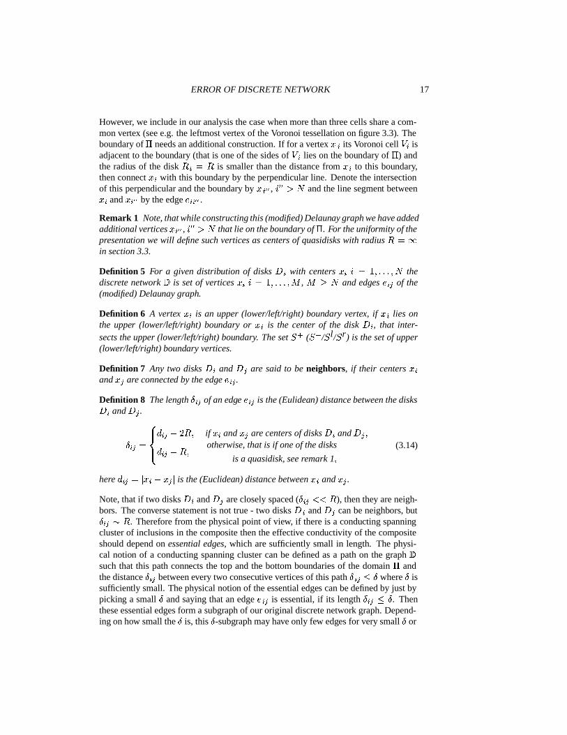
However, we include in our analysis the case when more than three cells share a com-mon vertex (see e.g. the leftmost vertex of the Voronoi tessellation on figure 3.3). Theboundary of * needs an additional construction. If for a vertex � # its Voronoi cell

� # isadjacent to the boundary (that is one of the sides of

� # lies on the boundary of * ) andthe radius of the disk � #�� is smaller than the distance from � # to this boundary,then connect � # with this boundary by the perpendicular line. Denote the intersectionof this perpendicular and the boundary by �7#�� , - � � � . and the line segment between� # and � # � � by the edge � ## � � .Remark 1 Note, that while constructing this (modified) Delaunay graph we have addedadditional vertices � # � � , - � � � . that lie on the boundary of * . For the uniformity of thepresentation we will define such vertices as centers of quasidisks with radius � � �in section 3.3.

Definition 5 For a given distribution of disks ! # with centers � # - � � # . . . # . thediscrete network

�is set of vertices � # - � � # . . . # � ,

� � . and edges � # � of the(modified) Delaunay graph.

Definition 6 A vertex � # is an upper (lower/left/right) boundary vertex, if � # lies onthe upper (lower/left/right) boundary or � # is the center of the disk ! # , that inter-sects the upper (lower/left/right) boundary. The set � � ( � � / � l/ � r) is the set of upper(lower/left/right) boundary vertices.

Definition 7 Any two disks ! # and ! � are said to be neighbors, if their centers �N#and � � are connected by the edge � # � .Definition 8 The length ��# � of an edge � # � is the (Eulidean) distance between the disks!$# and ! � .

� # � � �� P # � � 5 � # if � # and � � are centers of disks ! # and ! � #P # � � � # otherwise, that is if one of the disks

is a quasidisk, see remark 1 #(3.14)

hereP # � � � � # � � � � is the (Euclidean) distance between � # and � � .

Note, that if two disks ! # and ! � are closely spaced ( � # � �� ), then they are neigh-bors. The converse statement is not true - two disks ! # and ! � can be neighbors, but� # �� . Therefore from the physical point of view, if there is a conducting spanningcluster of inclusions in the composite then the effective conductivity of the compositeshould depend on essential edges, which are sufficiently small in length. The physi-cal notion of a conducting spanning cluster can be defined as a path on the graph

�such that this path connects the top and the bottom boundaries of the domain * andthe distance � # � between every two consecutive vertices of this path � # � � � where � issufficiently small. The physical notion of the essential edges can be defined by just bypicking a small � and saying that an edge � # � is essential, if its length �Q# � � � . Thenthese essential edges form a subgraph of our original discrete network graph. Depend-ing on how small the � is, this � -subgraph may have only few edges for very small � or


a lot of edges if � is sufficiently large (see figure (3.4)). In particular, the 2-subgraphis the whole discrete network, because the distance to the boundary for any interiordisk is always � 5 . On the other hand there is a small � � , so that the � � -subgraphdoes not have any edges at all. If ��= � �9? , then the ��= -subgraph is nested in the ��? -subgraph, that is every edge of the ��= -subgraph is also an edge in the � ? -subgraph,but not vice-versa. The 2-subgraph has the largest number of edges among all the � -subgraphs. For the 2-subgraph vertices of every pair of neighbors are connected, andthe 2-subgraph typically triangulates the domain * . When � � 5 , this is not necessar-ily true any more; however, when � is not very small the � -subgraph still partitions thedomain into polygons. The size of these polygons measures the connectivity propertiesof in the composite: if these polygons have a lot of edges, then the connectivity prop-erties of the composite are poor; if, on the other hand, these polygons have few edges,then the connectivity properties of the composite are good. In the latter case using theintuition from the case of periodic square and hexagonal lattices we expect, that thefluxes between the closely spaced disks will play the dominant role in the computationof the effective conductivity. Hence we wish to study these connectivity propertiesof � -subgraphs. The graph-theoretical concept of the minimal cycles accurately cap-tures the idea of the size of the polygons in the partition of * by the � -subgraph. Aminimal cycle on a (sub)graph is a closed path, that cannot be shortened by replacingsome edges of this path by other edges of the (sub)graph. As usual, the situation atthe boundary needs a special treatment. At the boundary we need to consider “bound-ary” paths. These are the paths, that start on the boundary and end on the boundary.For a boundary path a minimal cycle is again the one that cannot be shortened. Theseconnectedness properties of � -subgraphs are used in the in section 4 for error estimatesof the discrete network approximation. Therefore, for completeness, in the rest of thissection we give the precise graph-theoretical definitions related to this notion. Most ofthem are taken from [5].

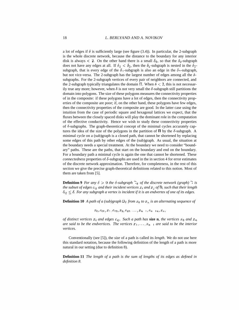
Definition 9 For any � � % the � -subgraph��

of the discrete network (graph)�

isthe subset of edges � # � and their incident vertices � # and � � of

�, such that their length� # � � � . For any subgraph a vertex is incident if it is an endvertex of one of its edges.

Definition 10 A path of a (sub)graph� �

from � � to �� is an alternating sequence of

� � # � � = # � = # � = ? # � ? # � ? ; # . . . # �� = # � � � =�� # �� #of distinct vertices � # and edges � # � . Such a path has size n, the vertices � � and ��are said to be the endvertices. The vertices � = # . . . # �� = are said to be the interiorvertices.

Conventionally (see [5]), the size of a path is called its length. We do not use herethis standard notation, because the following definition of the length of a path is morenatural in our setting (due to definition 8).

Definition 11 The length of a path is the sum of lengths of its edges as defined indefinition 8.


Definition 12 An internal cycle�

of� �

is an alternating sequence of� � # � � = # � = # � = ? # �@? # � ? ; # . . ./�� # � � � # � � #of vertices and edges, such that� � # � � = # � = # � = ? # � ? # � ? ; # . . ./� �is a path, and � � � connects the vertices � � and � � . Such a cycle has size n+1.

Definition 13 A boundary cycle�

of� �

is a path� � # � � = # �N= # � = ? # � ? # � ? ; # . . . �� #such that the endvertices � � and � � lie on the boundary of the domain * . Such aboundary cycle has size n.

Note that the endvertices � � and � � of a boundary cycle may lie on different parts ofthe boundary of the domain * , for example left and upper.

Definition 14 A minimal cycle�

m is a (internal or boundary) cycle, such that for anytwo vertices � # and � � of this cycle the shortest path from � # to � � is a subset of thecycle

�m. If the cycle

�m is a boundary cycle, we also require that for any interior

point � # of this cycle the shortest path from to � # to any point � � on the boundary is asubset of the cycle

�m.

Note that we require for a minimal boundary cycle an additional condition. This con-dition guarantees that a boundary cycle cannot be shortened by connecting an interiorpoint of this cycle with the boundary.

Definition 14 is a formalization of an intuitive notion of a hole in a composite. Eachhole in a composite is surrounded by a loop of conducting disks (see figure 1.1 (a)). Onthe modified Delaunay graph this loop corresponds to an � -gon, which is a minimalcycle of this graph.

Definition 15 The size of the largest minimal cycle � of a (sub)graph� �

is the upperbound on the size of all its minimal cycles, that is

�'� E��m �

�� size � � m � (3.15)

where�

m is a minimal cycle.

Definition 16 The interior of a cycle�

is a polygon having the cycle�

as its bound-ary, that is

Int � � � .

The degree of the connectedness of the whole graph�

can now be quantified interms of the two parameters: � and � , and an a priori relative error estimate for thediscrete network approximation

�will be determined in terms of these parameters only.

Definition 17 A discrete network (graph)�

is � - � connected if


(i) for every vertex � # of the graph�

there exists a minimal cycle�

of its � -subgraph� �such that � # � Int � , where Int � , the interior of a cycle

�.

(ii) the size of the largest minimal cycle of� �

is � .

Condition (i) in definition (17) implies that if � , � and � are not too large, thenthere exists at least one path on the graph

� �such that it connects the top and the

bottom boundaries of the domain * . This can be shown by contradiction using theduality argument. Suppose there are no paths on the graph

� �that connect the top and

the bottom boundaries. Then there exists a path in the whole domain * such that itconnects the left and the right boundaries of * and does not intersect

� �. The length

of this path on the one hand must be larger than the distance between the left and theright boundaries, on the other hand it cannot be larger than the diameter of the largestminimal cycle. Recall that the distance between any two vertices in

�does not exceed5 � � � , hence the inequality the inequality

5�2 � � 5 � � � � � � 5 (3.16)

must hold. But inequality (3.16) cannot hold if � ,�

and � are not too large, thereforewe have a contradiction. The existence of a path on

� �which connects the top and the

bottom boundaries means the existence of the conducting spanning cluster, since thedistance �Q# � between every two consecutive vertices of this path satisfies ��# � � � bydefinition of

� �.

3.3 The triangle-neck partition

Here we describe an algorithm that leads to a construction of the partition of the do-main & ( (defined by (2.1)) into non-overlapping subdomains. This algorithm is thetriangle-neck partition of the domain & ( induced by the Voronoi tessellation. It is anauxiliary construction, which is used in section 4 as a convenient and efficient tool forthe construction of the trial functions for the error estimates. The main goal is to havea decomposition of & ( into simple geometric figures - necks and triangles only, suchthat necks between neighbors must be included into the decomposition. By means ofthis decomposition we will able to account for the idea of Keller that the flux is impor-tant only in necks between almost touching disks. This decomposition also makes thederivation of variational error estimates transparent.

The main idea of the triangle-neck partition is to connect two neighbors ! # and ! �by a neck * # � . The widths of these necks are chosen so that after we connect all theneighbors, the domain * is partitioned into necks * # � and polygons. These polygonsare typically triangles. If they are not triangles, we partition them further by essentiallydrawing diagonal lines.

Here is the precise algorithm. For a given distribution of disks ! # , -�� # . . . #/.construct the Voronoi tessellation and the discrete network�

as in section 3.2. Con-sider any two neighbors !D# and ! � with centers � # and � � respectively (see figure3.5(a)). Denote by � and ( the endpoints of the common edge of their Voronoi cells� # and

� � . For each � connect the center � � with all the vertices of its Voronoi cell� � by auxiliary line segments (see dotted lines on figure 3.5(a)). Denote by � � � the


x i

x j

x k

xl

x

Ain

A kn

A jn

On

m

Op

A

A

A

A

lp

mp

jp

ip A

A

A

A

ip

lp

mp

kp

∆

∆

∆

ijk

ikl

lnk

Π

Π

ik

jkA

A

in

jn

(a) Voronoi tessellation (b) Triangle-neck partition

Figure 3.5: Decomposition of Voronoi cell

intersection of the line segment � � � with the circumference of the disk ! � . Definesimilarly points � # � and � � � . Connect the points � # � , � � � and � � � .

Definition 18 The neck * # � between the neighbors ! # and ! � is the curvilinear quad-rangle � # � � # ( � � ( � � � , bounded by the two line segments � # � � � � and � # ( � � ( and thetwo arcs �)# � � # ( and � � � � � ( .

Typically a neck * # � is not symmetric with respect to the line connecting the centersof the disks ! # and ! � . An example of a neck is given on figure 3.1 where we usedthe local coordinate system where the centers of the both disks lie on the � -axis. In thiscoordinate system the width of the left half-neck is

� �C= � , � = � % , and the width of theright half-neck is

� � ? � , �N? � % . Note that inequalities �"= � % � ? � % are not true ingeneral, but �5= � �N? always by our construction.

Definition 19 The maximal and the minimal relative half-neck widths are defined by

��# � � E�� = �� # � � ? �� # �� # � � E$FG � � � = �� # � � ? �� # % � �� # � � ��# � � �1.(3.17)

We use the relative half-neck widths� ��# � and

� �� # � in the error estimates in section4.

When we apply this algorithm to all neighbors, in general, all these line segments�)# � � � � partition the domain & ( into necks * # � between neighboring disks and trian-gles

� # � � (see figure 3.5(b)). In degenerate (exceptional) cases instead of triangles weobtain polygons (for example quadrangle � # ( � � ( � � ( � � ( on figure 3.5(b)) which can


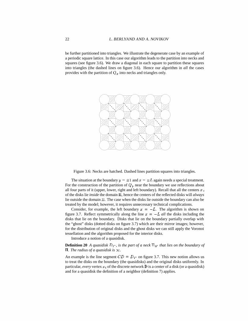
be further partitioned into triangles. We illustrate the degenerate case by an example ofa periodic square lattice. In this case our algorithm leads to the partition into necks andsquares (see figure 3.6). We draw a diagonal in each square to partition these squaresinto triangles (the dashed lines on figure 3.6). Hence our algorithm in all the casesprovides with the partition of & ( into necks and triangles only.

Figure 3.6: Necks are hatched. Dashed lines partition squares into triangles.

The situation at the boundary � �� and � �� 2 again needs a special treatment.For the construction of the partition of & ( near the boundary we use reflections aboutall four parts of it (upper, lower, right and left boundary). Recall that all the centers � #of the disks lie inside the domain * , hence the centers of the reflected disks will alwayslie outside the domain * . The case when the disks lie outside the boundary can also betreated by the model; however, it requires unnecessary technical complications.

Consider, for example, the left boundary � � �32 . The algorithm is shown onfigure 3.7. Reflect symmetrically along the line �-��32 all the disks including thedisks that lie on the boundary. Disks that lie on the boundary partially overlap withthe “ghost” disks (dotted disks on figure 3.7) which are their mirror images; however,for the distribution of original disks and the ghost disks we can still apply the Voronoitessellation and the algorithm proposed for the interior disks.

Introduce a notion of a quasidisk.

Definition 20 A quasidisk ! # � � , is the part of a neck * #H# � that lies on the boundary of* . The radius of a quasidisk is � .

An example is the line segment� !�� !D# � � on figure 3.7. This new notion allows us

to treat the disks on the boundary (the quasidisks) and the original disks uniformly. Inparticular, every vertex � # of the discrete network

�is a center of a disk (or a quasidisk)

and for a quasidisk the definition of a neighbor (definition 7) applies.


Definition 21 The triangle-neck partition� � � � & (�� of the domain & ( is the set of

necks * # � and triangles� # � � .

The triangle-neck partition is unique up to partitioning of degenerate (exceptional)polygons into triangles. The necks * # � connect two disks (in particular, a disk anda quasidisk) ! # and ! � if they are neighbors. All vertices of the triangles lie on thecircumferences of the disks (or quasidisks).

Since from the physical point of view, for a discrete network�

the necks of its� -subgraph carry the main information about the effective properties of the material,we wish to show that all the triangles and the “non-essential” (longer than � ) necks donot contribute to the discrete network approximation. In order to do that, we need anestimate on the number of such non-essential necks and triangles in the triangle-neckpartition relative to the number of essential (shorter than � ) necks.

Remark 2 For a given distribution of disks there is the one-to-one correspondencebetween its discrete network

�and the associated triangle-neck partition where the

necks *3- � are associated with the edges � # � , and the triangles� # � � are associated with

the respective ( -cycles of the graph�

. Therefore we will use instead of the edges � # �the corresponding necks * # � where there is no confusion.

The next lemma gives an upper bound on the number of necks and triangles that liein the interior of any minimal cycle of the � -subgraph in terms of the size of largestminimal cycle � . Consider a � - � connected discrete network

�(definition 17).

Consider a minimal cycle�

m of the � -subgraph� �

. Denote by � � �m the number

of the triangles� # � � that lie in the interior of this minimal cycle

� # � �� Int � m.Similarly � * � m is the number of the necks * # � that lie in the interior of this minimalcycle * # �� Int � m, and � � � m is the number of the vertices (centers of disks) � # suchthat � # � Int � m.

Lemma 1 Suppose the discrete network�

is � - � connected. Then for any minimalcycle

�m of the � -subgraph

� �the number of triangles � � �

m, and the number ofnecks � * � m that lie in the interior of

�m satisfy the bounds

� � �m� 5 � � � 5� � ( �

? � #� * � m

� ( � � � 5� � ( �? � . (3.18)

Proof: Consider a cycle�

m. By Euler’s formula

� � �m �� * � m �� m �&�1. (3.19)

Since each triangle has three edges and each edge belongs to at most two triangles

(�� m� 5�� * � m . (3.20)

Therefore

� � �m� 5/�� * � m ��

m � � 5�� m #� * � m

� � � m �� m� (�� m . (3.21)


If�

m is a minimal cycle of� �

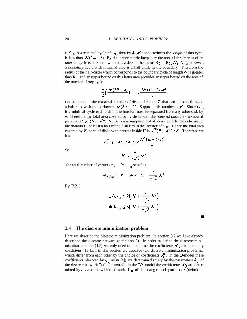
, then by � - � connectedness the length of this cycleis less than �� 5 � � � � . By the isoperimetric inequality the area of the interior of aninternal cycle is maximal, when it is a disk of the radius R � � R � �!� # � # � � ; however,a boundary cycle with maximal area is a half-circle at the boundary. Therefore theradius of the half-circle which corresponds to the boundary cycle of length . is greaterthan R � . and an upper bound on this latter area provides an upper bound on the area ofthe interior of any cycle

�5 � �� 5 � � � �� ? �)5 � ? � � � � � 51� ?� .

Let us compute the maximal number of disks of radius � that can be placed insidea half-disk with the perimeter �� 5 � �� . Suppose this number is � . Since

�m

is a minimal cycle each disk in the interior must be separated from any other disk by� . Therefore the total area covered by � disks with the (densest possible) hexagonalpacking is 5 � ( �*� �$� � 51� ? � . By our assumption that all centers of the disks lie insidethe domain * , at least a half of the disk lies in the interior of

�m. Hence the total area

covered by � parts of disks with centers inside * is� (6�*� � � � 5 � ? � . Therefore we

have� (6� � � � � 51� ? � � 5 � ? � � � � � 51� ?�

So

� � 5� � ( �? .

The total number of vertices � #5� �Q� � � m satisfies

� � � m� � � � � � � 5� � ( �

? .By (3.21)

� � �m� 5 � � � 5� � ( �

? � #� * � m

� ( � � � 5� � ( �? � .

3.4 The discrete minimization problem

Here we describe the discrete minimization problem. In section 3.2 we have alreadydescribed the discrete network (definition 5). In order to define the discrete mini-mization problem (1.5) we only need to determine the coefficients � �# � and boundaryconditions. In fact, in this section we describe two discrete minimization problems,which differ from each other by the choice of coefficients � �# � . In the

�-model these

coefficients (denoted by ��# � as in [4]) are determined solely by the parameters ��# � ofthe discrete network

�(definition 5). In the

� �-model the coefficients � �# � are deter-

mined by ��# � and the widths of necks * # � of the triangle-neck partition�

(definition


xx

x

x x

x

x=−L

ii’

j’

k’ k

j

C

D

A

A

A

A

k’ k

ii’

B

quasidisk

Πiixi’’

D i’’

Figure 3.7: Vertical boundary

21). The�

-model is simpler, because it does not use the widths of necks *D# � , but theerror estimates for the

� �-model are better.

Let us begin here with the�

-model. For a given distribution of disks ! # withcenters � # , - � � # . . . #/. define the discrete network

�with vertices � # - � � # . . . # � ,� � . and edges � # � . For

� � � �B/= # �B ? # . . . # �B � � consider

� � � �+� �� 2 � �� # � � �B # � �B � � ? . (3.22)

Here the summation is over all necks * # � . The relative interparticle fluxes � # � aredefined by (3.5). The discrete potentials

�B # at the “boundary” vertices � # , are prescribedon the horizontal boundaries by

�B # �� for � # �:� � # (3.23)

where � � are the upper/lower boundary vertices (definition 6).The discrete potentials

�B # at the “interior” vertices � # � �� Q� # # - � � # . . . #/. �� A� � � , are the values of discrete potentials. If a vertex of the discrete network� # � �� '� � � , then � # � must be a center of a quasidisk, that lies on the left or

the right boundary � # � �5� � l �D� r. For such vertices we assume

�B # � �� B # (3.24)


where B # is the value of the potential on the disk ! # � � �-� � � � � � � , B # � � is thevalue of the potential on the quasidisk ! # � � connected with the disk ! # (on figure 3.7!$# � � � � ! ).

The discrete minimization problem is to find the potentials at the interior vertices,that is a set of

� ��B # � �@# � � � , such that the quadratic form (3.22) with conditions(3.23),(3.24) is minimal, that is

E FG�B # # � # � �� (6.85 (%� # � (6.85 � �� )� � � . (3.25)

Definition 22 If � ��B/# � �@#3� � � is the solution of the discrete minimization problem

(3.25), then

� � � � �� 2 � �� # � ��B # � B � � ? (3.26)

is the energy of the discrete network for the�

-model.

The discrete network is a connected graph in the sense that there is a path betweeneach vertex � # and a boundary vertex � � �8� � . This implies that the discrete mini-mization problem has a unique solution, because if a graph is connected, then any localminimizer of the quadratic form (3.22) is the (unique) global minimizer. Therefore wehave

Lemma 2 There is a unique solution � �QB # � � # � � � of the discrete minimization

problem (3.25). This solution satisfies a discrete analog of Euler-Lagrange equations(compare to (2.5)) � �� # fixed

��# � ��B # � B � � � % for all �@#5� � . (3.27)

Since the quadratic form (3.22) is positive-definite the proof follows immediately fromlinear algebra.

Remark 3 The summation in (3.27) is over necks * # � , such that one of their endpoints� # is fixed. All these necks must be incident to the vertex � # . In the sequel we will usethe same notation.

The values B � �# , for � � �# �� '� � � play no role in the minimization process andcan be determined a posteriori by (3.24). In particular we will need the following� �� # � � fixed

� # � � � ��B # � � � B � �+� � # � � # ��B # � � � B # �+� % for all � # �� D� � � . (3.28)

Denote by� � and

� � the discrete fluxes (confer to (2.6)) through the boundaries� � and � � respectively� ��

� �� # � ��B # � B � � (3.29)

� ��

� �� # � ��B # � B � � .


Then� � �&� � � � �5 � �� # � ��B # � B � � ? ��5 2 � � � # (3.30)

where the first and the second equalities are the discrete analogs of formulas (2.6) and(2.12) respectively. The derivation of (3.30) uses (3.27) and the following rearrange-ment of terms. The first equality

� � � � � � holds, because

� � � � �� # � ��B # � B � � � � �� # � ��B # � B � �� # � ��B # � B � �� # � ��B # � B � � � � �� # � ��B # � B � � � � �� # � ��B # � B � � � � � � .

The second equality in (3.30) can be deduced from (3.27) and (3.28)

� 2+� � � � � �� # � ��B # � B � � ? � � �� # � ��B # � B � � ��B # � B � �� B #/0 � �� # fixed

��# � ��B # � B � � 4�� B � 0 � �� fixed

� � # ��B � � B # � 4� � � �� B # 0 � �� # fixed

��# � ��B # � B � � 4�� B � 0 � �� fixed

� � # ��B � � B # � 4� � �� # � ��B # � B � � � � �� # � ��B � � B # � � � � � � � .

Lemma 3 Discrete maximum principle. Suppose ��B = # B ? # . . . B � � is the solution

of the�

problem (3.25). For any (internal or boundary) cycle�

of�

define

B �� E�� B # � # � # � � # B �� E$FG ��B # � # � # � � .Then for any vertex � � with potential B � such that � � � Int � , that is � � belongs to theinterior of the cycle

�(see definition 16) we have

B �� B � � B �� .Proof: The proof of the discrete maximum principle is by contradiction, and it is

fairly standard. Suppose not all the values B # for the points � # in the interior of the cycleare the same and the maximum of B # is achieved in the proper interior of the cycle at apoint �A� Int � # � � �� . Then we have � # � �� for any � # � Int � . Therefore, thediscrete Euler-Lagrange equation (3.27) is satisfied only if B # � B� whenever vertices�@# and � are connected by a neck * # . Hence the maximum is also achieved at all thepoints �@# which are connected with � by a neck * # . Since the graph is connected,the induction over all the points in the interior of the cycle implies the contradiction:the values B/# for all the points in the interior of the cycle are the same.As a corollary of the discrete maximum principle we have


Lemma 4 If the discrete network�

is � - � connected, then for any minimal cycle�

of the � -subgraph� �

and a vertices � � � Int � and � � � Int � we have

��B � � B � � ? � � � �� m

��B # � B � � ? # (3.31)

Proof: By the discrete maximum principle (lemma 3)

��B � � B � � ? � ��B �� B �� ? (3.32)

where B �� E�� B # � # � # � � # B �� E$FHG ��B # � # �@#5� � .By the triangle inequality for the values of the potentials B # , � # � �

��B �� B �� ? � � � �� m

��B # � B � � ?which inserted in (3.32) yields (4).

Let us discuss now the� �

-model. For a given distribution of disks !A# � # , - �� # . . . #/. define the discrete network�

with vertices � # -�� # . . . # � ,� � . and

edges � # � and the triangle-neck partition�

(definition 21). Then the specific fluxes � �# �can be determined by formula (3.4) in terms of necks *D# � . Then, similar to the firstmodel, we define

� � � � � � �� 2 � �� # � � �B # � �B � � ? # (3.33)

and the second discrete minimization problem: find a set ��B # � � # � � � , such that

E$FHG�B # # � #5� ��*(6.85 (%� # �*(6.85 � �� # (3.34)

here the energy of the discrete network for the� �

-model

��!� � � � �� 2 � �� # � ��B � # � B �� ? . (3.35)

For the second discrete minimization problem one can derive properties similar to lem-mas 2, 3, equation (3.27) etc. Quantities

� �� similar to� � can be defined as well. Let

us compare the two discrete minimization problems for quadratic forms

� � � � �� 2 � �� # � ��B # � B � � ?and

� �1� �+� �� 2 � �� # � ��B # � B � � ? .


By (A.17) � �# � � � # �therefore for any

� �� B = # �B ? # . . . �B � � we have

� �%� � � � � � � �Hence E$FG�B # # � # � ��*(/. 5 (1� # �*(/. 5 � �

��%� � � � E$FHG�B # # � # � ��*(6.85 (%� # �*(6.85 � �� . (3.36)

Suppose E$FHG � �%� � and E$FG � � � is achieved on the sets � � �QB � = # B � ? # . . . B � � � and ��B = # B ? # . . ./B � � respectively. Then

� � �+� �� 2 � �� # � ��B # � B � � ? � �� 2 � �� # � ��B � # � B �� ? � �� 2 � �� # � ��B � # � B �� ?� �� 2 � �� # � � � �# � � ��B � # � B �� ? � � � � � � � �� 2 � �� # � � � �# � � ��B � # � B �� ? .

Hence

� �1� � � � � � � � ��!� � �� 2 � �� # � � � �# � � ��B � # � B �� ? .In the cases we consider here ( � - � connectedness, definition 17) we show in section4 a tighter inequality

� � � � � � � � � � �� " �� .4 Variational bounds on the effective conductivity

The classical approach to variational bounds is to find some “good” trial functions<�� ( and v � � ( and apply inequality (2.16). The main difficulty is to find the trialfunctions. A successful choice of the trial functions leads to tight bounds. The idea ofconstructing tight bounds by means of variational principles is not new and have beenused by many authors but each time the main question is the actual construction ofdual test functions which is usually highly nontrivial and it relies on specific featuresof the problem. For example, the test functions for the dual bounds from [8] or [16]are very different from ours and from each other due to different geometries. Thereis no general recipe for choosing the trial functions. In this section we show that forour specific problem of effective conductivity of high contrast, highly packed particularcomposites we can construct the upper and the lower bounds for a composite when itsdiscrete network

�is � - � connected (definition 17) and we estimate the difference

between the upper and the lower bounds in terms of � , � and the energies � � � and� � � � of the discrete minimization problems (equations (3.26) and (3.35)). This allowsto give an estimate on the relative error between the effective conductivity (2.9) and the


energy of the discrete network (3.26). Certainly our trial functions give upper and lowervariational bounds on effective conductivity for any distribution of disks; however, ourbounds are tight only under the assumption that “almost all” the distances �@# � betweenneighbors are sufficiently small ( � - � connectedness).

Definition 23 A distribution of disks ! # , - � � # . . . #/. satisfies the � - � close packingcondition if its discrete network

�is � - � connected.

We also give a better estimate on the relative error between the effective conduc-tivity (2.9) and the energy of the discrete networks (3.26), (3.35) in two special cases:�2� ( and � � � . If � � ( , then all neighbors are � -close to each other. Thecase �'�)( covers distributions of disks which are small perturbations of the periodichexagonal lattice (figure 3.2), therefore it is important for applications. If � � � thenthe condition that all neighbors are � -close is relaxed. In particular, this case includesthe periodic square lattice (figure 3.6).

Here is the the idea of the construction of the variational bounds. Our goal is toconstruct two trial functions, which mimic the behavior of the solution to the mini-mization problem (3.34) for the

� �-model. The domain * consists of disks ! # , necks* # � and triangles

� # � � where the necks and triangles are determined by the triangle-neck partition. The function < � � ( and the function v � �A( are defined first on thedisks, then in the necks and the triangles. Suppose B � # are the values of the solution ofthe minimization problem (3.34) for the

� �-model. The function < � � ( is chosen

so that it takes the values B � # on the disks ! # , it is equal to �� on the boundaries � �and it is linear in the necks. Observe that the formulation of the problem is rotationallyinvariant, therefore in the construction of the trial functions we routinely locally rotatethe plane so that in the local coordinates a particular neck * # � is always aligned withthe vertical direction. The function < should be piecewise-differentiable by definitionof the space

� ( (2.2). Therefore on triangles it is defined by linear interpolation. Thefunction v � � ( intuitively is the flux of < , and it is chosen on disks and necks takinginto account the discrete fluxes of the discrete minimization problem. The function vdoes not have to be piecewise-differentiable, hence we simply define it to be zero onthe triangles.

The idea of the error estimate is to show that both the upper and lower bound arevery close to the energy of the

� �-model. In order to show that the energy of the

�-

model (3.25) is a good approximation as well we compute the difference between thesolution of the

� �-model and the solution of the

�-model.

4.1 The lower bound

The test function v for the lower bound is chosen to be zero everywhere except thenecks * # � between adjacent disks. Consider two neighbors centered at � # and � � .The potentials B � # and B �� on the disks ! # and ! � are the solutions to the minimizationproblem (3.34) for the

� �-model. Rotate the domain so that in the local coordinates

the neck between them is aligned with the direction of the � -axis. Define

v �� % # �� HQ� � in the neck * # � #� % # % � otherwise,

(4.1)


where � �� is the distance between the disks (figure 3.1). Let us check that the testfunction v lies in the space � ( defined by (2.13). If at x � * # � then divergence-freecondition amounts to O � v(x) �

� % �)��B � # � B ��

� �� % .If x � � # � � (see figure 4.2), thenO � v(x) �

� % �

�% � % .

If a point x lies on the boundary of the triangle-neck triangulation, that is x � * # �� # � , the vector field v is discontinuous there. In this case the divergence-free condi-tion amounts to checking that the normal components of v match along the discontinu-ity. This matching is satisfied trivially for v. The condition

J �� v � n P x � %is satisfied due to (3.4). Indeed, we have

J �� v � n P x � �� B � # � B �� J � �� P �� # � ��B � # � B �� % .

Here the last sum is zero for any - � � by (3.27). By the quasidisk construction (3.28)the condition

v � � 2 #� �� n � %is also satisfied. Observe that for the trial function (4.1) the fluxes through the upperand the lower boundary of * are exactly the discrete fluxes

� �� and� �� for the

� �-

model J � � = v � n P x � � � � � � � �# � ��B � # � B �� #J � � � = v � n P x � � � � �� # � ��B � # � B �� .

Therefore similar to (3.30)

J � � = v � n P x � J � � � = v � n P x � � �� # � ��B � # � B �� ? (4.2)

The value of the integral over the neck * # � is

J �� v ?9P x � ��B � # � B �� ? J � �� P �� # � ��B � # � B �� ? #

and J L M v ?QP x � � �� # � ��B � # � B �� ? . (4.3)


By (4.2) and (4.3)

J�� = v � n P x � J�� = v � n P x � �5 J L M v ?QP x � �5 � �� # � ��B � # � B �� ? .Hence we have a lower bound

Proposition 4.1 The lower bound on � � in terms of � �# � and the parameters of the solu-tion of the discrete minimization problem is

� � � � � � �� 2 � �� # � ��B � # � B �� ? � � �/. (4.4)

We remark here that the left-hand side in (4.1) is always positive, which reflects thephysics of the problem. The analogous lower bound in Proposition 2.1 in [4] is positiveand it is sufficiently tight for the � - ( close packing condition only. Our bound allowsus to handle general distribution of disks that satisfy � - � close packing condition forany � .

4.2 The upper bound

x

y

1 2

x

x

Π ij

j

i

δij

xo

H(x )/2o

S S

Figure 4.1: A typical neck between two disks.


φ=

φ=

t i

t j

x i

φ= t kA

B

CO

xj

x k

K

0

0

0

Figure 4.2: Typical� �� # � � , half-necks are hatched.

Consider a piecewise continuous test function < . The function < is linear in y in theneck * # � with the values B � # and B �� on the boundary of the disks

! # and ! � (figure

4.1). Then on the neck * # �< �� #� �+�8B � # � ��B �� B � # � � � � � �� 5 �� 8B � # �)��B �� B � # � � �� 5 � #for � � 0 � � �� 5 #

� �� 5 4 . (4.5)

The function < is linear in the� # � � (see figure 4.2) with the values B � # , B �� and B � � at the

vertices of� # � � . On figure 4.2 these vertices are the points � , � and

�respectively.

The estimates on the� L M � O < � ? P x depend on the bounds on the relative half-neck

widths� ��# � ( see (3.17)) for closely spaced neighbors ! # and ! � . Such estimates

are derived in appendix A.1 for the � - � closely packed disks. These estimates areuniform for fixed � and � , that is

� ��# � � � � � # (4.6)

where�

is a number independent of - and � , computed in appendix A.1. Assumption(4.6) for all practical cases usually satisfied with much better estimates than our worstcase scenario estimates in (A.2)-(A.4) (lemma 6). By (A.19) and (A.11) and (4.6) wehave


Proposition 4.2 The upper bound on � � in terms of � �# � and the parameters of the solu-tion of the discrete minimization problem is

� � � �� 2 � �� # � � �� G �� G 50 � ��B � # � B �� ?� �� 2 5� � � � ? �

� �� B � # � B �� ? �)��B � � � B � # � ? � . (4.7)

4.3 The error estimate

As we already mentioned, the error of approximation of the minimization problemof effective conductivity (2.9) by the energy of

� �-model (3.25) is based solely on

propositions 4.1 and 4.2, where if we assume the non-degenerate case (that is all thetriangles

� # � � are adjacent to three necks * # � , * � � and * � # ), then we have

�� 2 � �� # � ��B � # � B �� ? � � � � �� 2 � �� # � � Const � ��B � # � B �� ? #where Const �

� � G � � � � � � � � � � G 50 �� ? �� as � � % . (4.8)

Equation (4.8) simply reflects the fact that the effective conductivity � � is the sum of theintegrals in the � -direction over all necks (here we use our local coordinate systems),the sum of the integrals in the � -direction over all necks and the sum of the integralsover all triangles. The sum of the integrals in the � -direction over all necks is equivalent

to the energy � of the�

-model (3.26) and therefore it is � � � � � as � � %. The sum

of the integrals in the � -direction over all necks and the sum of the integrals over alltriangles is �� as � � %

(see appendices A.2 and A.4 respectively). Similar to (4.8)we have an error estimate between the energies of the

� �-model and the

�-model

�� 2 � �� # � ��B � # � B �� ? � �� 2 � �� # � ��B # � B � � ?� �� 2 � �� # � ��B � # �AB �� ? � �� 2 � �� # � � � �# � � ��B � # � B �� ? #

where� � # � � � �# � � � � �� by (A.17) .

(4.9)

Hence the idea of the proof: we wish to “absorb” all the � �� terms in (4.8) and

(4.9) as the “smaller order corrections” into � � � � � the terms and derive an estimate

� � � � � � � �� " �� .

Then we have � � ��

� �" �� . (4.10)


The main goal of the theorems in this section is to evaluate � in (4.10).

Theorem 4.3 Under the � - � close packing condition (definition 23) for � � � � (15the relative error � � � � ��

� � � 56. � 0 � � " �� . (4.11)

where the effective conductivity

� � � �� 2 J�L M � O < � ?�P x #�� 2 J LNM � O < � ?�P x � �� 2 E$FHG�I �� M J L M � O �< � ?�P x

and the energy of the� �

-model

� � �)� � � � � �� 2 � �� # � ��B � # � B �� ? #�� 2 � �� # � ��B � # � B �� ? � �� 2 E$FG��

� �� # � � �B � # � �B �� ? .Remark 4 The factor � � (%5 in theorem 4.3 is chosen for the simplicity of presentationand it is not essential. If our estimates on

� � # � � � �# � � in appendix A.3 and the proof oftheorem 4.3 are modified, the statement of theorem 4.3 is true for any � � � .

Proof: By proposition 4.1, the effective conductivity � � is bounded from below

� � � � �+� �� 2 � �� # � ��B � # � B �� ? � � � .By proposition 4.2, the effective conductivity � � is bounded from above

� � � ��%� � �� B � # � B �� ? � � �� B � # � B �� ? (4.12)

Where the last two summations in (4.12) are respectively over all neck and triangles ofthe triangle-neck partition. Our goal is to bound (4.12) by the following sum

�� 2 � �� # � � �� B � # � B �� ? � �� 2 � �� # � ��B � # � B �� ? (4.13)

where� �

is the � -subgraph of the discrete network�

(definition 9). Since� �# � � � � � �# � � � � � " �� # when * # � � � � (4.14)

we obtain (4.11). The basic reason for deducing (4.13) from (4.12) is that the keyrelation (4.14) is guaranteed only for the necks of the � -subgraph

� �. Full graph

�may contain ”long” necks, for which (4.14) does not hold.

The proof of the theorem consists of three basic estimates


� For any minimal cycle�

m recall the notation

– � � �m is the number of triangles

� # � � , such that� # � � � Int � m,

– � * � m is the number of necks, * - � such that * # � � Int � m,

– � � � m is the number of vertices � # , such that � # � Int � m.

By lemma 1

� � �m� 5 � � � 5� � ( �

? ��#� * � m

� ( � � � 5� � ( �? � . (4.15)

� By the analog of lemma 4 for� �

-model for every � � � Int � m and � � � Int � mwe have

��B � � � B �� ? � � � �� m

��B � # � B �� ? . (4.16)

� Using the estimates (4.15), (4.16) and (A.4) in proposition 4.2 we have

� � � �� 2 � �� # � � �� G � � � � � � � � � � G 50 �6��B � # � B �� ?� �� 2 5� � � � ? �

� �� 1��B # � B � � ? �)��B � � B # � ? �� 2 � �� # � ��B � # � B �� ? � �� 2 � �� B � # � B �� ?6 � � �# � � � � � � 5� � ( �

? � � 5 5 5� � � � ? � (� � G � � � � � � � � � � G 50 � �

� �� 2 � �� # � ��B � # � B �� ? � �� 2 � �� # � � � � 5 .�� 0+� � " �� B � # � B �� ?� �1� � 5 .�� 0 � � " �� 2 � �� # � ��B � # � B �� ? � �1� � 5 .�� 0 � � " �� .

Here 5 .�� 0 � � is a uniform upper bound on

" �� # � � � � 5� � ( �

? � � 515 5� � � � ? � (� � G �� G 50 � .

Therefore

�� 56. � 0 � � " �� (4.17)


or % � � �3� �� 56. � 0 � � " �� 1.Hence � � � � � � �

�� 56. � 0 � � " �� .Theorem 4.4 Under the � - � close packing condition for � � � � (15 the relative error

� � �3� � ��

� �/. ,%5 � � " �� . (4.18)


� � � �� 2 J LNM � O < � ?�P x #�� 2 J�LNM � O < � ?�P x � �� 2 E$FHG�I �� M J�L M � O �< � ?�P x

and the energy of the�

-model

� �)� � � � �� 2 � �� # � ��B # � B � � ? #�� 2 � �� # � ��B # � B � � ? � �� 2 E$FG��

� �� # � � �B # � �B � � ? .Proof: Using (4.9) and (A.17) we have

�� 2 � �� # � ��B � # � B �� ? �-� �%� � � � � � � (4.19)

and

� � � � �� 2 � �� # � ��B � # � B �� ? � �� 2 � �� # � � � �# � � ��B � # � B �� ? (4.20)

The length of the largest neck � # � can be bounded by means of the maximal size of theminimal cycles of the � -subgraph

� �. We have

��# � � � � � � � � 51� � �� (4.21)

Similar to the proof of (4.11), by (3.31), (3.18), (4.21) and (A.17) inequality (4.20)


gives

� � � � �� 2 � �� # � ��B � # � B �� ? � �� 2 � �� B � # � B �� ?6 � � �# � � ( � � � � 5� � ( �

? � � � � � (5 � 5" �� 0 � �

� �� 2 � �� # � ��B � # � B �� ? � �� 2 � �� # � � � � �6. ,15 � � " �� B � # � B �� ?� �1� � �/. ,%5 � � " �� 2 � �� # � ��B � # � B �� ? � �1� � �/. ,%5 � � " �� %� � � .

Therefore

� � � � � � � �/. ,%5+� � " �� . (4.22)

By (4.20), (4.22) and (4.17)

� � � �� E�� /. ,%5+� � # 5 .�� 0 � � � " �� 6. ,15 � � " �� 0 � � " �� .

Hence � � � ��

� �6. ,15 � � " �� .The constants 56. � 0 � �� in (4.11) and �/. ,%5 � �� in (4.18) are very rough

upper bounds on the relative errors and they could be significantly improved by morecareful analysis. We give now a better estimate on the relative errors in two specialcases: �'�)( and � � � .Theorem 4.5 If � �)( and � � � � (15

� � �� (6. , �

" �� . (4.23)


� �� 2 J L M � O < � ? P x #�� 2 J LNM � O < � ?QP x � �� 2 E$FG�I�� M J L M � O �< � ?QP x



-model

� � �)� � � � � �� 2 � �� # � ��B � # � B �� ? #�� 2 � �� # � ��B � # � B �� ? � �� 2 E$FG��

� �� # � � �B � # � �B �� ? .Proof: Using (A.22) and (A.2) in the variational bound (4.7) (proposition 4.2) we

have

� � � �� 2 � �� # � � �� G � � � � � � � � � � G 50 � 5 �� ( � � � �5 � � �6��B � # � B �� ?

� �1� � (6. , � " �� 2 � �� # � ��B � # � B �� ? � � � � (6. , � " �� %� � � .Hence � � � �� %� � � � � � " �� !��B � � # or

� � ��

" �� .

Theorem 4.6 If � � ( and � � � � (15� � � � � ��

� ,/. 01," �� . (4.24)


� � � �� 2 J�L M � O < � ?�P x #�� 2 J LNM � O < � ?�P x � �� 2 E$FHG�I �� M J L M � O �< � ?�P x


-model

� �)� � � � �� 2 � �� # � ��B # � B � � ? #�� 2 � �� # � ��B # � B � � ? � �� 2 E$FG��

� �� # � � �B # � �B � � ? .Proof: By (A.17) and (4.9)

��%� � � � � � � � �� 2 � �� # � � ,/. 01, �� B � # � B �� ? � �� (6. , � " �� !� � � .


Therefore

� � � �� E�� *,/. 01, # (6. , � � " �� ,/. 01, " �� .Theorem 4.7 If � � � and � � � � (15

� � � �� 56.87 (

" �� . (4.25)


� �� 2 J L M � O < � ?QP x #�� 2 J LNM � O < � ? P x � �� 2 E$FG�I�� M J L M � O �< � ? P x


-model

�� )��%� �+� �� 2 � �� # � ��B � # � B �� ? #�� 2 � �� # � ��B � # � B �� ? � �� 2 E$FG��

� �� # � � �B � # � �B �� ? .Proof: Using (A.23) and (A.3) in the variational bound (4.7) (proposition 4.2) we

have

� � � �� 2 � �� # � � �� G �� G 50 � 0 � 5 � � � �5 � � �/��B � # �AB �� ?

� � � � ��5 . 7�( " �� 2 � �� # � ��B � # � B �� ? � � � � ��5 . 7�( " �� %� � � .Hence � � � �� %� � � � � ��5 . 7�( " �� !� � � # or

� � � �� 56.87 (

" �� .

Theorem 4.8 If � � � and � � � � (15� � � ��

� (156.87 �" �� . (4.26)


� �� 2 J L M � O < � ? P x #�� 2 J LNM � O < � ?QP x � �� 2 E$FG�I�� M J L M � O �< � ?QP x



-model

� �)� � � � �� 2 � �� # � ��B # � B � � ? #�� 2 � �� # � ��B # � B � � ? � �� 2 E$FG��

� �� # � � �B # � �B � � ? .Proof: When � � � the maximal ��# � is

� 5/� 5 � � � � � 5 � . By (A.17) and (4.9)

� � � � � � � � � � �� 2 � �� # � � (%5 . 7 � �� 6��B � # � B �� ? � � � � � . ( " �� .Therefore

� � �� E�� *(%5 . 7 � # ��56.87 (1� " �� (156.87 � " �� .Remark 5 Asymptotically as � � %

both models (�

-model and� �

-model) give thesame values of the effective conductivity, in the sense that

� � �+�� " �� #� � � � � � � � �) � �� #

� � � � � � % � " � � � # � � � � � � � � � � � �� #� � � � � � � � � � �� # as � � % .(4.27)

Since in the� �

-model we take into account more geometry of the original continuousproblem, it may seem that the

� �-model gives a better approximation to the effective

conductivity than the�

-model. However, due to the errors that arise when we integrateperpendicular to the necks (see (A.7)) the errors of both models are compatible. Morespecifically, the

�-model approximates the Dirichlet’s integral in a neck

J �� O < � ? P x � J �� < � � ? P x � J �� < � � ? P x (4.28)

by � # � ��B # �8B � � ? , where � # � is given by the Keller’s asymptotic formula (3.5). Thisasymptotic formula neglects the value of the first term on the right-hand side of (4.28)and approximates the second term of (4.28). On the other hand, in the

� �-model we

compute the second term of the Dirichlet’s integral (4.28) exactly, but we neglect thefirst term of it. When � � %

the value of this second term in (4.28) is compatible to theerror of the Keller’s approximation (3.5) of the first term, hence the

� �-model does not

provide with the approximation of the effective conductivity which is better than the oneof the

�-model. This means that for the purpose of estimating the effective conductivity

of a composite where inclusions are almost touching each other both models are equiv-alently good; however, the

� �-model also provides with a rigorous lower variational

bound on the effective conductivity even if � is not small, because � �!� � � � � � .


4.4 A numerical illustration

The main goal of this paper is to give a rigorous quantitative justification of discretenetwork model (1.5) by means of a priori error estimates. However, the use of our trialfunctions for the upper and the lower bounds gives a numerical a posteriori error. Wemust solve the discrete network problem (3.25), construct the trial functions <�� ((see section 4.1) and v � �A( (see section 4.2) and evaluate explicitly the left-hand sideand the right-hand side of the upper and lower bound (2.16). The evaluation of this dualbound is not computationally expensive, because we use simple trial functions - theyare given by explicit analytic formulas on the necks and they are linear interpolationson the triangles. This section implements this idea for numerical simulations of arandomized hexagonal lattice.

The algorithm for these simulations consists of three parts:

� An algorithm for a numerical simulation of a randomized hexagonal distributionof disks.

� An algorithm for a numerical evaluation of the dual variational bounds.

� Statistics.

Let us discuss these three parts in more detail.Distribution of disks. The distribution of disks is implemented by randomization

of a periodic hexagonal lattice of disks of equal radii � #�� % . % 5 on a squaredomain 0 � � # � 4"6 0 � � # �94 , and then removal of some fraction of these disks from thisdistribution. More specifically:

� Choose a volume fraction � .

� By formula (3.12) determine the corresponding interparticle distance � for thechosen volume fraction � .

� Distribute disks of radius � # �� % . % 5 with the computed interparticle dis-tance � periodically on a square domain 0 � � # � 4"6 0 � � # �94 as in figure 3.2. Thecenters of the boundary disks may not lie exactly on the boundary, but as wehave already remarked this makes insignificant corrections to the effective con-ductivity.

� Randomize the hexagonal periodic distribution of disks by shifting the centers ofall the disks by a random vector. We chose to shift each centers of a disk inde-pendently by a vector with a length that has a uniform distribution on an interval0 % # � � (1�Q4 and with a direction that has a uniform distribution on 0 % # 5 � 4 . This ran-domization guarantees that the distance between neighbors � # � �A0 � � (1� # � � ( �Q4 .

� Choose a volume fraction �� of disks to be removed. Compute thenumber of disks to be removed and then remove this number randomly withuniform probability. This removal procedure typically creates holes of size � �0 , if �� is small.


0 10 20 30 40 50 60 70 800

10

20

30

40

50

60

simulation run

Iφ, f

r=0

I, fr=0

I, fr=0.3

Iφ, f

r=0.3

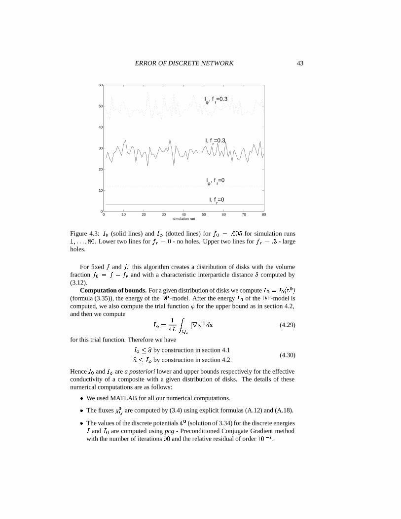
Figure 4.3: � � (solid lines) and � I (dotted lines) for � � � . 0 % � for simulation runs� # . . . # ,%. Lower two lines for � � � % - no holes. Upper two lines for � � ��. ( - large

holes.

For fixed � and � � this algorithm creates a distribution of disks with the volumefraction � � � �$�� and with a characteristic interparticle distance � computed by(3.12).

Computation of bounds. For a given distribution of disks we compute � � �)��1� � �(formula (3.35)), the energy of the

� �-model. After the energy � � of the

� �-model is

computed, we also compute the trial function < for the upper bound as in section 4.2,and then we compute

� I � �� 2 J L M � O < � ? P x (4.29)

for this trial function. Therefore we have

�� by construction in section 4.1

� � � � I by construction in section 4.2 . (4.30)

Hence � � and � I are a posteriori lower and upper bounds respectively for the effectiveconductivity of a composite with a given distribution of disks. The details of thesenumerical computations are as follows:

� We used MATLAB for all our numerical computations.

� The fluxes � �# � are computed by (3.4) using explicit formulas (A.12) and (A.18).

� The values of the discrete potentials � (solution of 3.34) for the discrete energies� and � � are computed using pcg - Preconditioned Conjugate Gradient method

with the number of iterations � % and the relative residual of order � % � �

.


� After � are determined, � I is evaluated using explicit formulas (A.8) (A.21).

The computation of �� and � I is fast, therefore it allows to study the statistics of theeffective conductivity.

Statistics. The simulations are done with the% . % � increments of � � . For fixed �

and � � there were , % simulations. For the mean we use the notation

� � �!� � � �� = � � # (4.31)

where � � is the result of � -th simulation with fixed � and � � and the number of simu-lations � �), % .

0.1 0.2 0.3 0.4 0.5 0.6 0.7 0.8 0.9 10

20

40

60

80

100

120

volume fraction f0

E(Iφ), f

r=0

E(I), fr=0

E(I), fr=0.3

E(Iφ), f

r=0.3

Figure 4.4:� �*� � � (solid lines) and

� �*� I � (dotted lines) as functions of the volumefraction � � � % . � % � # . . . % . � % � . Lower two lines for the case with no holes. Upper twolines for the case with holes.

Results. Here we present the results of the numerical simulations that show thedependence of the effective conductivity on the presence of holes in the matrix.

On figure 4.3 we plot �� (solid lines) and � I (dotted lines) for all , % simulationswhen the volume fraction of the inclusions is fixed � �� % . 0 % � and � � takes two val-ues � � � % and � � � . ( . The case � � � % corresponds to the case when there areno holes in the material. The case � � ��. ( corresponds to almost maximal possiblenumber of holes for this volume fraction in the sense that before removal of disks thevolume fraction � � % . � % � is very close to the densest possible (hexagonal) packing.Indeed, the volume fraction of the periodic hexagonal packing when disks touch is� � ( � 0 � % . � % 01, . . . . Observe that for the same total volume fraction � � � % . 0 % �for all numerical simulations a distribution of disks with holes has greater effective


conductivity than a distribution of disks without holes, because the lower bound � � onthe effective conductivity for a distribution of disks with holes is always larger than theupper bound � I on the effective conductivity for a distribution of disks without holes.

On figure 4.4 we plot� � � � � (solid lines) and

� � � I � (dotted lines) as functions of thevolume fraction � � � % . � % � # . . . % . � % � . The volume fraction of removed disks � � takestwo values � � � % and � �3� . ( . Observe that in the presence of holes the a posteriorierror of the network approximation � I � � � is significantly larger than in the case whenthere are no holes. For example when � � � .�� in the presence of holes the a posteriorierror is (/. � times larger than the error in the case when there are no holes.

If the total volume fraction of the inclusions is fixed, then the increase of the vol-ume fraction of holes in the material implies that the interparticle distance � decreases.Hence the percolation effects play a more significant role. Therefore we expect that forhighly packed composites the relative error of our discrete model is smaller in the casewhen there are holes compared with the case when there is no holes. Indeed, when� �� . 0 the relative a posteriori error for composites with holes is up to , times betterthan relative error for composites with no holes for the same volume fraction. When� � � . ( � the effective conductivities of a material with holes and of a material with-out holes are numerically very close, at least the computed a posteriori error does notallow to distinguish between these composites. For such volume fractions there are nopercolation effects in both cases.

Remark 6 Let us compare the a posteriori error estimates discussed in this sectionand the a priori error estimates given in section 4.3. Suppose we want to compute themaximal interparticle distance � such that the error of the discrete network approxima-tion is less than � %�� . Consider the case of a quasi-hexagonal lattice ( � ��( ). From(4.23) the a priori error estimate is" �

�� . � # therefore � � 06. 7�, � � % � � ��.

So the a priori error estimate guarantees a � %�� accuracy if � is about � � %�% timessmaller, than the radius of the disks � .

The a posteriori error estimate can be computed from our numerical simulationsfor a quasi-hexagonal distribution of disks with no holes (see the lines that correspondto � � � % on figure 4.4). These simulations show, that a � %�� accuracy is achieved if �is about 5�� % times smaller, than the radius of the disks � .

Therefore the use of the a posteriori error widens the range of the characteristicdistance � , where the discrete network gives a good approximation.

5 Conclusions

In this paper we derived an explicit a priori error estimate for the network approxima-tion (the

�-model) introduced in [4] for the effective conductivity of a high contrast

highly packed composite under the so-called � -close packing-conditions. Furthermore,the approach developed in this paper allowed us to consider much more generic ge-ometrical arrays of the particles which satisfy the so-called � - � close packing con-dition. Roughly speaking the first condition means that all the neighboring particles


are closely spaced whereas the second condition allows for strongly non-uniform ge-ometrical arrays when a significant fraction of the particles does not participate in theconducting cluster. We have shown quantitatively how such nonuniformity affects theerror estimate and therefore the quality of the approximation.

We have also introduced and justified the modified network approximation (the� �

-model) which generalizes the network approximation from [4]. This modified networkapproximation is no longer asymptotic in nature. Roughly speaking we decomposethe Dirichlet integral (1.4) for the effective conductivity into two parts: the networkapproximation ,which is a quadratic form and the error term. Our modified networkapproximation accounts for all fluxes between the neighboring particles, where neigh-bors are defined via Voronoi tessellation. If the fluxes are small (neighbors are notclosely spaced), then the corresponding coefficients in the modified network approxi-mation (1.9) are not significant but unlike [4] we do not need to introduce any cut-offdistance in the numerical implementation. For the both network approximations (the�

-model and the� �

-model) the error term is explicitly estimated based on the con-struction of the trial functions using the triangle-neck partition of the domain. Thecomparison of the error terms in the two models shows that the a priori estimate in the� �

-model is about 5 .�� ( times better than that for the�

-model which makes a bigdifference in practical computations.

Finally we provide model examples of numerical implementation of the networkapproximation. We observe that irregularity in the geometrical distribution of the in-clusions in all simulations consistently lead to a significant (up to � % times) increase inthe effective conductivity at the same total volume fraction of the inclusions. We alsoobserve numerically that our network approximation works better for irregular geomet-ric patterns, which are not quasi-hexagonal, that is when a typical number of nearestneighbors can vary significantly. In our model example for the same volume fraction ofinclusions (larger than . 0 ) the the relative a posteriori error estimate in the presence ofholes in the conducting cluster is up to , times better than for uniformly highly packedcomposites.

Thus we conclude that both approximations provide a very efficient computationaltool for evaluation of the effective properties of high contrast composites, which is ca-pable of capturing the effects of irregular geometrical arrays with a good control of theapproximation error. We expect that the method developed in this work will be gener-alized for more complicated problems of highly packed elastic and fluid composites.

A Appendix. Auxiliary estimates

A.1 Estimates on the relative neck widths

Here we give upper and lower bounds on the relative half-neck widths� ��# � and

� �� # � .Recall that ( see (3.17))

� ��# � � E�� = � � � # � � ? � � � � # � �� # � � E FG � � � = � � � # � �N? � � � � .Lemma 5

� �� # � � E�� % # � � �5 � � � � # �5 � � ? � (A.1)


δ

x

x

x j

O

i

kij

Figure A.1: The worst case scenario for the lower bound on� �� # � .

Proof: For any distribution of centers � # , � � and � � � �� # � is larger than the oneshown on figure A.1. In the latter case

� �� # � �� FHG � � � # � � � �� FG � � 5 � 5 � � � � # �� 5�� FG ? � � � � � # �+�&� � �5 � � � � # �5 � � ? .

Lemma 6 If� �)(

� ��# � � � � �5 � �� 5 � ? . (A.2)

If� � �

� ��# � � � � � �5 � �� 5 � ? . (A.3)

If�

is arbitrary��# � � � � 5 � �

� � � � � 5 � � � ? . (A.4)


x

x j

x

δ

δ

O

i

k

Figure A.2: The worst case scenario for the upper bound on� ��# � when

� �)( .

Proof: The upper bound on� ��# � depends on the distribution of other disks. By

definition all the vertices � of the Voronoi tessellation (see figure 3.5) are centers oftriangle’s

� � # � � � � circumcircles (in degenerate cases instead of a triangle� � # � � � �

we may have � -gons) such that no other vertices � # of the Delaunay graph�

are con-tained inside these circumcircles. The upper bound on

� ��# � is determined by theestimate on the maximal possible diameter of these circumcircles.

In the case� � ( the largest

� ��# � is shown on figure A.2. Here the half-neckbetween the disks ! # and ! � is the largest possible. Since �� 5 � � �N#�� @#�� therefore

� # � �� FHG � � # � � � � � 5�� FG ? � � # � � � � � 5 � �5 � � � � ? � � � �5 � �

� � � � 5 � ?In the case

� � � the largest half-neck� # � between disks ! # and ! � is shown on

figure A.3. In this case� � � � # � � � � �� 45 � � � . Therefore the maximal possible

diameter of the circumcircle is� 56� 5 � � � � . Since

� � #�� 5 � then

� ��# � � � � � � �� 5 � 5 � � � � � 5 �

? � � � � �5 � �� 5 � ? .


x

x

x

xl

j

A

B

Ci

k


� � � .

In the case when�

is arbitrary the diameter of the maximal circumcircle is boundedby a half of the length of the largest minimal cycle. On figure A.4 � # � � is this diameterand we have � � # � � � � �*� � � � 51�/� .The largest half-neck on figure A.4 is between � # and � � . We have

� ��# � �� FG � � 5 � � � # � � � � � �� # � � � � � � � � 5 � ��*� � � � 5 � � � ? .

A.2 Gradient estimates inside the necks

The gradient of < �� #� � on the neck * # � is given by

< � � � � ��B �� B � # � � � � �� ? ��

< � � � B �� B � #� �� . (A.5)


x

x

x

i

j

k


�is arbitrary.

By (A.5)

J �� < � � � ? P � P � � J � �� B �� B � # � ?� ? �� P � � ��B �� B � # � ? � �# � (A.6)

where � �# � is defined in (3.4). Also

J �� < � � � ?QP � P � � J �� B �� B � # � ? � � � � �� ? �� ? P � P �

� J �� B �� B � # � ? � � � �� ? �� ? � ;( � � �HQ�� ?� � �� ? P � � ��5 ��B �� B � # � ? J �� ? ��

� �� P � .(A.7)

Since � �� )� � 5 �)� 5 � � ? � � ? , therefore � � �� +� ? � � � � � and

� � ? �� ?

� ? � � ? �� 5 � � 5 � � ? � � ? �

5� ? � � ? � ?

�)� � � ? � � ? � 5� ? � � ? �*� � � � ? � � ? � � 5 �

� ? � � ? � 5� � ? � � ? #

(A.8)

J � �� 5 �� ? � � ? P � � J � �� 5

� � ? � � ? P � � � � G � �,��)� � � 5 � � � � FG ��

��

�� (A.9)


then from (A.7), (A.8) and (A.9) we have

J �� < � � � ? P � P � � �� 5 ��B �� B � # � ? J � �� ? �� P � �

��5 ��B �� B � # � ? � 5 � G 5

� � � ��# � � 5 � � � � � G �� # � � � � � � � G 50 ��B �� B � # � ? (A.10)

where� ��# � is defined by (3.17). Combining (A.10), (A.6) the value

� �� O < � ? P x is

J �� O < � ?�P x � ��B �� B � # � ? � � �# � � � � G �� # � � � � � � � G 50 � . (A.11)

A.3 Comparison of fluxes for the two discrete networks

Here we establish a relation between the relative interparticle flux � # � (3.5) and thespecific flux ��# � (3.4). Consider the case of a disk and a quasidisk � # �-� , � � �)� .

� �� +� � # � � �)� � � ? � � ? .With the change of variables

� �)� � � � �� FG � � � � � � # � � � � � � # 5� �� 5 � � �� 56.we have� �# � � J � �� P �

�9# � � �)� � � ? � � ? � J �� P ��9# � � �)��

� J �� # � � � � �� # � � �)� � � � � � � P �

� J �� 9# � � � � �� # � � 5 � � FG ? � � 5 � P �

� J �� 5/�*��# � � � � � � � # �� ? � � 5 �)�� 5 � � � # � � � FG ? � � 5 � P �

� � � � � 5 ��# � � �� # � � � � 5 � � �9# � � � = ? � � �� G � �� 5 � � �9# � � = ? � � G � � � 5 � � ��

�� 5 � # � � �

� � ?# � � 5 � � # � �� G � � � ?# � � 5 � � # � � � G � � � 5 �� # � � � ��

�� (A.12)


For each � � � # 5% � � 5 � � � �� G � � 5 � � �9# �� # � � � G � � � �� 51� � � �� G � � �9# �

5 � � � # � � � � � � � �� 51� �� E FG � " ��# �5 � � � � � � � �� 51� # � 5 � � E$FHG � " �9# �5 � � � � � � � � �� # � � ?� �� # � #

�5 � .

(A.13)

Using (A.1) we have

�5 � � � �� G � � 5 � � � # �

��# � � ��G � � � �� 5 � � � E$FHG � " � # �5 � � �6. � � ( � # �� # � 5 � . (A.14)

Also

% � ��# � � �� ?# � � 5 � ��# � � � �

5 � # �� # � � # � � � � � � � # � � 5 � � ?� � � 5 �� # � ( � 5 � � � # �

� # � � � � � � � # � � 5 � � ? � � ��# � � 5 � � (� � 5" � # ��

(A.15)

and we obtain for any � # �� # � � � �# � � � � 5 ��# � � � � � � 5 � # � � �

� � ?# � � 5 � � # � �� G � � � ?# � � 5 � � # � � � G � � � 5 ��# � � � ��

��

� � � 5 �9# � � �� ?# � � 5 � ��# � � � 5 �� # � � �� G � � � ?# � � 5 � � # � � � G � � � 5 �� # � � � �

��

�� 5 ��9# � � �

5 � �� G � � � ?# � � 5 � �9# � � � G � � � 5 ��# � � � ��

� �� 5 �� # � � �

5 � �� G � � � ?# � � 5 � �9# � � � G � � � 5 �� # � � � ��

��(A.16)

Combining (A.14), (A.15) and (A.16) we have

% � ��# � � � �# � � � � � (5 � 5" �9# �� 5 �� # � E$FG � " ��# �5 � � � .�� (1�9# �� # � 5 �


Combining (A.14), (A.15) and (A.16)

% � � # � � � �# � � � � � (5 � 5" ��# �� E FG �1� �6. � � ( ��# �� # � 5 � 5 �� # � � (A.17)

The case of two disks with equal radii � #��)� � �)� follows from (A.17), because theproblem of two disks with equal radii becomes equivalent to solving two problems for adisk and quasidisk with the length � # � � 5 when we draw the middle-point perpendicularto the line which connects centers of the disks(the x-axis on figure 3.1). Analogous to(A.17) we derive estimates for the case � # �-� � � � with

� �� +�)�9# � � 5 � � 5 � � ? � � ? .For such � �� formula (A.12) is

� �# � � � � �

5 �� # � � 5 �

� � ?# � � � � � # � � � �� G � � � ?# � � � � �9# � � ��G � � � 5 ��9# � � � ��

�� . (A.18)

However, these new estimates are more tight than (A.17), therefore we must use(A.17) for an estimate independent of radii of the disks. Observe that the estimate(A.17) is valid for any � # � . The estimate (A.17) implies that the term � # � is the leadingterm in the asymptotic expansion of � �# � if � # � is small and the width � ? � � = is non-small. Observe that if � # � is small it implies that the width of the neck is non-small(estimate (A.1) on

� �� # � ).

A.4 Gradient estimates inside the triangles

Lemma 7

J � �� O < � ?QP x � 5� � � � ? �%��B # � B � � ? �)��B � � B # � ? �where

� � � �� E�� # � # � �� # � �� # � . (A.19)

Proof: By construction the Voronoi tessellation induces the triangle neck partitionof the domain * . Each triangle is (typically) bounded by three (half)necks. On figure4.2 we show a typical case with three disks centered at � # , � � and � � , three half-necksand the

� � � � � � # � � bounded by these half-necks. The potential < is defined at thevertices of

� � � � < � � �+�8B #< � ��+�8B �< � � � �+B � . (A.20)

Since < is a piecewise continuously differentiable define < on� �� by linear inter-

polation of these three values. Suppose in� �� the side

� � � � is the longest, andthe side

�� is the shortest ( see figure 4.2). Then

% � � � � �@#�� ( ,


� � � � � � � � �� 5 , � � � �� , and the endvertex of the perpendicular � � on thebase � � lies between the points � and

�. Suppose that < � �$� �8B � . Then we haveB � � B #B � � B # � � �� #

therefore B � �+B # � ��B � � B # � � �� Denoting by

� � � � � the area of� �� we have

J �� O < � ? P x �� B � � B �� ? � � B # � B ��

? � � � � � �� FG � � � � � �

5 � � ��B # � B � ��)��B � � B # � � �� FG � � � � � � � ? � � B # � B �� ? �

�� FG � � � � � �

56 � � ��B # � B � � �� FHG � � � � � � �)��B � � B # � � �� FHG � � � � � � �?�

� B # � B �� ? �� FG � � � � � �

6 �%��B # � B � � ? �� ? � FG ? � � � � � � � ��B � � B # � ? � � � � � ? � � � � � �� ? �� FHG � � � � � � �1��B # � B � � ? � � � �� )��B � � B # � ? � ��

� 5� FHG � � � � � � � ��B # � B � � ? �)��B � � B # � ? � .

(A.21)

Hence J �� O < � ?QP x � 5� FHG � � � � � � �1��B # � B � � ? �)��B � � B # � ? � �

In terms of the parameter� � � �� we have a bound

�� FG � � � � � � �

�� FG � �� 5 � � � � � � � � �

� � � � � �� ? .therefore J �� O < � ?QP x � 5� � � � ? � ��B � # � B �� ? �)��B � � � B � # � ? � .

By lemma 6 we have

Corollary 1 Assume� �� E�� # � # � �� # � �� # � .


If �'�)(J � �� O < � ? P x � �

� ( � � � �5 � � � ��B � # � B �� ? �)��B � � � B � # � ? � . (A.22)

If �'� �

J � �� O < � ? P x � 5 � 5 � � � �5 � � � ��B � # � B �� ? � ��B � � � B � # � ? � . (A.23)

If � is arbitrary

J � �� O < � ? P x � �� ? �1� � �5 � � �%��B � # � B �� ? �)��B � � � B � # � ? � . (A.24)

References

[1] Ambegaokar, V., Halperin, B.I., Langer, J,S. 1971, Hopping conductivity in dis-ordered systems. Phys.Rev.B, 4(8), pp2612-2620 (1971).

[2] Bakhvalov N. S., Panasenko G. P., Homogenization: averaging processes in pe-riodic media. Kluwer, Dordrecht (1989).

[3] Bensoussan A., Lions J-L., Papanicolaou G., Asymptotic Analysis for PeriodicStructures, North-Holland, Amsterdam, 1978.

[4] Berlyand, L., Kolpakov, A., Network approximation in the limit of small inter-particle distance of the effective properties of a high contrast random dispersedcomposite, Arch. Ration. Mech. Anal. 159 (2001)3, pp. 179-227.

[5] Bollobas, B., Modern graph theory. Graduate Texts in Mathematics, 184.Springer-Verlag, New York, 1998.

[6] Borcea, L., Asymptotic Analysis of Quasistatic Transport in High Contrast Con-ductive Media. SIAM Journal on Applied Mathematics, 59:2(1999), pp.597-639.

[7] Borcea L., Berryman J.G., Papanicolaou G., Matching pursuit for imaging highcontrast conductivity. Inverse Problems, 15:4(1999), pp.811-849.

[8] Borcea, L., Papanicolaou G., Network approximation for transport properties ofhigh contrast materials. SIAM J Appl Math, 58:2(1998), pp.501-539.

[9] Borcea L., Papanicolaou, G., Low frequency electromagnetic fields in high con-trast media. Surveys on Solution Methods for Inverse Problems, D. Colton, H.W. Engl, A. Louis, J. R. McLaughlin, W. Rundell editors, Springer Vienna/NewYork, 2000.

[10] Bruno, O., The effective conductivity of strongly heterogeneous composites. Proc.Royal Soc. London A, 433(1991), pp. 353-381.


[11] Clerc, J.P., Giraud, G., Laugier, J.M., Luck, J.M., The electrical conductivityof binary disordered systems, percolation clusters, fractals and related models.Advances in Physics, 39:3(1990), pp. 191-309.

[12] Ekeland, I., Temam, R.,Convex Analysis and Variational Problems. North Hol-land, 1976.

[13] Halperin, B.I.,Remarks on percolation and transport in networks with a widerange of bond strengths, Physica D, 38(1989), pp. 179-183.

[14] Keller, J.B., Conductivity of a Medium Containing a Dense Array of PerfectlyConducting Spheres or Cylinders or Nonconducting cylinders. J. Appl. Phys.,34:4(1963), pp. 991-993.

[15] Koplik, J., Creeping flow in two-dimensional networks. J. Fluid Mech.,119(1982), pp. 219-247.

[16] Kozlov, S.M., Geometrical aspects of averaging, Russ. Math. Surveys,44:2(1989), pp. 91-144.

[17] McPhedran, R. Transport property of cylinder pairs of the square array of cylin-ders, Proc. R. Soc. London. A, 408(1986), pp. 31-43.

[18] McPhedran, R., Poladian.L, and Milton, G.W. Asymptotic studies of closelyspaced, highly conducting cylinders, Proc.. R. Soc. Lond. A, 415(1988), pp. 185-196.

[19] McPhedran, R., Milton, G.W. Transport properties of touching cylinder pairs andof the square array of touching cylinders. Proc. R. Soc. London A, 411(1987), pp.313-326.

[20] Schwartz, L.M., Banavar, J.R., Halperin, B.I., Biased-diffusion calculationsof effective transport in inhomogeneous continuum systems, Physical review B,40:13(1989), pp. 9155-9161.

[21] Shah, C.B., Yortsos, Y.C.,The permeability of strongly-disordered systems,Physics of Fluids, 8:1(1996) , pp. 280-282.

[22] Smythe, W. R., Static and dynamic electricity. 2nd edition, McGraw-Hill, NY,Toronto, London, 1950.

Date post:	22-Dec-2021
Category:	Documents
Upload:	others
View:	5 times
Download:	0 times

Error of the network approximation for densely packed ...

Documents