59
NCEE 2010-4004 Error Rates in Measuring Teacher and School Performance Based on Student Test Score Gains
NCEE 2010-4004
Error Rates in Measuring Teacher and School Performance Based on Student Test Score Gains
Error Rates in Measuring Teacher and School Performance Based on Student Test Score Gains July 2010 Peter Z. Schochet Hanley S. Chiang Mathematica Policy Research
Abstract This paper addresses likely error rates for measuring teacher and school performance in the upper elementary grades using value-added models applied to student test score gain data. Using realistic performance measurement system schemes based on hypothesis testing, we develop error rate formulas based on OLS and Empirical Bayes estimators. Simulation results suggest that value-added estimates are likely to be noisy using the amount of data that are typically used in practice. Type I and II error rates for comparing a teacher’s performance to the average are likely to be about 25 percent with three years of data and 35 percent with one year of data. Corresponding error rates for overall false positive and negative errors are 10 and 20 percent, respectively. Lower error rates can be achieved if schools are the performance unit. The results suggest that policymakers must carefully consider likely system error rates when using value-added
NCEE 2010-4004 U.S. DEPARTMENT OF EDUCATION
estimates to make high-stakes decisions regarding educators.

This report was prepared for the National Center for Education Evaluation and Regional Assistance, Institute of Education Sciences under Contract ED-04-CO-0112/0006. Disclaimer The Institute of Education Sciences (IES) at the U.S. Department of Education contracted with Mathematica Policy Research to develop methods for assessing error rates for measuring educator performance using value-added models. The views expressed in this report are those of the authors and they do not necessarily represent the opinions and positions of the Institute of Education Sciences or the U.S. Department of Education. U.S. Department of Education Arne Duncan Secretary Institute of Education Sciences John Q. Easton Director National Center for Education Evaluation and Regional Assistance Rebecca Maynard Commissioner July 2010 This report is in the public domain. While permission to reprint this publication is not necessary, the citation should be: Schochet, Peter Z. and Hanley S. Chiang (2010). Error Rates in Measuring Teacher and School Performance Based on Student Test Score Gains (NCEE 2010-4004). Washington, DC: National Center for Education Evaluation and Regional Assistance, Institute of Education Sciences, U.S. Department of Education. This report is available on the IES website at http://ncee.ed.gov. Alternate Formats Upon request, this report is available in alternate formats such as Braille, large print, audiotape, or computer diskette. For more information, please contact the Department’s Alternate Format Center at 202-260-9895 or 202-205-8113.

Disclosure of Potential Conflicts of Interest iii
Disclosure of Potential Conflicts of Interest The authors for this report, Dr. Peter Z. Schochet and Dr. Hanley S. Chiang, are employees of Mathematica Policy Research with whom IES contracted to develop the methods that are presented in this report. Drs. Schochet and Chiang and other MPR staff do not have financial interests that could be affected by the content in this report.

Foreword v
Foreword The National Center for Education Evaluation and Regional Assistance (NCEE) conducts unbiased large-scale evaluations of education programs and practices supported by federal funds; provides research-based technical assistance to educators and policymakers; and supports the synthesis and the widespread dissemination of the results of research and evaluation throughout the United States. In support of this mission, NCEE promotes methodological advancement in the field of education evaluation through investigations involving analyses using existing data sets and explorations of applications of new technical methods, including cost-effectiveness of alternative evaluation strategies. The results of these methodological investigations are published as commissioned, peer reviewed papers, under the series title, Technical Methods Reports, posted on the NCEE website at http://ies.ed.gov/ncee/pubs/. These reports are specifically designed for use by researchers, methodologists, and evaluation specialists. The reports address current methodological questions and offer guidance to resolving or advancing the application of high-quality evaluation methods in varying educational contexts. This NCEE Technical Methods paper addresses likely error rates for measuring teacher and school performance in the upper elementary grades using student test score gain data and value-added models. This is a critical policy issue due to the increased interest in using value-added estimates to identify high- and low-performing instructional staff for special treatment, such as rewards and sanctions. Using rigorous statistical methods and realistic performance measurement schemes, this report presents evidence that value-added estimates are likely to be quite noisy using the amount of data that are typically used in practice for estimation. If only three years of data are used for estimation (the amount of data typically used in practice), Type I and II errors for teacher-level analyses will be about 26 percent each. This means that in a typical performance measurement system, 1 in 4 teachers who are truly average in performance will be erroneously identified for special treatment, and 1 in 4 teachers who differ from average performance by 3 to 4 months of student learning will be overlooked. Corresponding error rates will be lower if the focus is on overall false positive and negative error rates for the full population of affected teachers. With three years of data, these misclassification rates will be about 10 percent. These results strongly support the notion that policymakers must carefully consider system error rates in designing and implementing teacher performance measurement systems based on value-added models, especially when using these estimates to make high-stakes decisions regarding teachers (such as tenure and firing decisions).

Contents Chapter 1: Introduction ............................................................................................................................ 1 Chapter 2: Statistical Framework for the Teacher-Level Analysis ........................................................ 3
The Basic Statistical Model and Assumptions .................................................................................. 3 Considered Estimators ....................................................................................................................... 6 Schemes for Comparing Teacher Performance ................................................................................. 8 Accounting for Tests From Multiple Subjects................................................................................. 10 Accounting for the Serial Correlation of Student Gain Scores Over Time ..................................... 11 Measuring the Reliability of Performance Estimators ..................................................................... 11 Calculating System Error Rates ....................................................................................................... 12
Chapter 3: Statistical Framework for the School-Level Analysis ........................................................ 17 Chapter 4: Simulation Analysis ............................................................................................................... 19
Obtaining Realistic Values for the Variance Components .............................................................. 19 Additional Assumptions for Key Parameters .................................................................................. 19 Identifying Threshold Values .......................................................................................................... 20 Simulation Results ........................................................................................................................... 22
Chapter 5: Summary and Conclusions ................................................................................................... 35 Appendix A .............................................................................................................................................. A-1 Appendix B .............................................................................................................................................. B-1 References .............................................................................................................................................. R-1
Contents vii

List of Tables ix
List of Tables
Table 4.1: Average Annual Gain Scores From Seven Nationally Standardized Tests ............................. 21 Table 4.2: Teacher-Level Analysis: Type I and II Error Rates that are Restricted to be Equal, by Threshold Value, Scheme, and Estimator .......................................................................... 23 Table 4.3: Reliability of the Teacher Value-Added Estimator, by the Number of Years of Available Data ......................................................................................................................... 24 Table 4.4: Teacher-Level Analysis: Overall False Positive and Negative Error Rates that Are Restricted to be Equal ....................................................................................................... 25 Table 4.5: Teacher-Level Analysis: The Number of Years of Data Required to Achieve Various System Error Rates for Scheme 2 .............................................................................. 26 Table 4.6: Teacher-Level Analysis: False Discovery and Non-Discovery Rates for Scheme 2 Using The Overall False Positive and Negative Error Rates in Table 4.4 .............................. 27 Table 4.7: Teacher-Level Analysis: Sensitivity of System Error Rates to Key ICC Assumptions and the Use of Multiple Tests .................................................................................................. 28 Table 4.8: School-Level Analysis: System Error Rates that Are Restricted to be Equal, by Threshold Value and Scheme .................................................................................................. 29 Table 4.9: School-Level Analysis: The Number of Years of Data Required to Achieve Various System Error Rates for Scheme 2 .............................................................................. 30


List of Figures xi
List of Figures
Figure 2.1: Hypothetical True Teacher Value-Added Measures ............................................................... 12 Figure 4.1: False Negative Error Rates and Population Frequencies for Scheme 2, by True Teacher Performance Level ....................................................................................... 32
Introduction 1
Chapter 1: Introduction
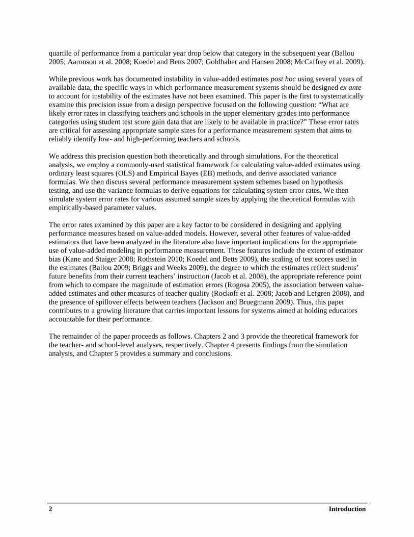
Student learning gains, as measured by students’ scores on pretests and posttests, are increasingly being used to evaluate educator performance. Known as “value-added” measures of performance, the average gains of students taught by a given teacher, instructional team, or school are often the most important outcomes for performance measurement systems that aim to identify instructional staff for special treatment, such as rewards and sanctions. Spurred by the expanding role of value-added measures in educational policy decisions, an emerging body of research has consistently found—using available data—that value-added estimates based on a few years of data can be imprecise. In this paper, we add to this literature by systematically examining—from a design perspective—misclassification rates for commonly-used performance measurement systems that rely on hypothesis testing. Ensuring the precision of performance measures has taken on greater importance with the proposal and implementation of policies that require the use of value-added measures for higher-stakes decisions. The most common application of these measures is to provide monetary bonuses to teachers or schools whose students have large learning gains (see Podgursky and Springer 2007). For instance, the Dallas Independent School District provides bonuses of $10,000 to teachers with high value-added estimates who agree to teach in the district’s most disadvantaged secondary schools (Fischer 2007; Dallas Independent School District 2009). In other schemes, even higher stakes have been proposed for the bottom of the performance distribution. A highly publicized proposal by Gordon et al. (2006) recommends that districts rank novice teachers on the basis of value-added estimates in conjunction with other types of measures at the end of their first two years of teaching, and that teachers in the bottom quartile of performance should generally not be rehired for a third year unless a special waiver is granted by district authorities. As the federal government prepares to channel more than $4 billion from the American Recovery and Reinvestment Act of 2009 (ARRA) into state education reforms, of which a prominent feature consists of “differentiating teacher and principal effectiveness” for determining compensation (U.S. Department of Education 2009), the use of value-added measures for policy decisions is likely to become even more widespread in the coming years. Given that individual teachers and schools can be subject to significant consequences on the basis of their value-added estimates, researchers have increasingly paid attention to the precision of these estimates. A number of studies have examined the extent to which differences in single-year performance estimates across teachers are due to persistent (or long-run) differences in performance—the types of differences intended to be measured—rather than to transitory influences that induce random error, and thus imprecision, in the estimates. As discussed by Kane and Staiger (2002a, 2002b), estimation error stems from two sources: (1) random differences across classrooms in unmeasured factors related to test scores, such as student abilities, background factors, and other student-level influences; and (2) idiosyncratic unmeasured factors that affect all students in specific classrooms, such as a barking dog on the test day or a particularly disruptive student in the class. As both sources of error are transitory, they are directly reflected in the amount of year-to-year volatility in a given teacher’s performance estimates. Existing research has consistently found that teacher- and school-level averages of student test score gains can be unstable over time. Studies have found only moderate year-to-year correlations—ranging from 0.2 to 0.6—in the value-added estimates of individual teachers (McCaffrey et al. 2009; Goldhaber and Hansen 2008) or small to medium-sized school grade-level teams (Kane and Staiger 2002b). As a result, there are significant annual changes in teacher rankings based on value-added estimates. Studies from a wide set of districts and states have found that one-half to two-thirds of teachers in the top quintile or
2 Introduction
quartile of performance from a particular year drop below that category in the subsequent year (Ballou 2005; Aaronson et al. 2008; Koedel and Betts 2007; Goldhaber and Hansen 2008; McCaffrey et al. 2009). While previous work has documented instability in value-added estimates post hoc using several years of available data, the specific ways in which performance measurement systems should be designed ex ante to account for instability of the estimates have not been examined. This paper is the first to systematically examine this precision issue from a design perspective focused on the following question: “What are likely error rates in classifying teachers and schools in the upper elementary grades into performance categories using student test score gain data that are likely to be available in practice?” These error rates are critical for assessing appropriate sample sizes for a performance measurement system that aims to reliably identify low- and high-performing teachers and schools. We address this precision question both theoretically and through simulations. For the theoretical analysis, we employ a commonly-used statistical framework for calculating value-added estimates using ordinary least squares (OLS) and Empirical Bayes (EB) methods, and derive associated variance formulas. We then discuss several performance measurement system schemes based on hypothesis testing, and use the variance formulas to derive equations for calculating system error rates. We then simulate system error rates for various assumed sample sizes by applying the theoretical formulas with empirically-based parameter values. The error rates examined by this paper are a key factor to be considered in designing and applying performance measures based on value-added models. However, several other features of value-added estimators that have been analyzed in the literature also have important implications for the appropriate use of value-added modeling in performance measurement. These features include the extent of estimator bias (Kane and Staiger 2008; Rothstein 2010; Koedel and Betts 2009), the scaling of test scores used in the estimates (Ballou 2009; Briggs and Weeks 2009), the degree to which the estimates reflect students’ future benefits from their current teachers’ instruction (Jacob et al. 2008), the appropriate reference point from which to compare the magnitude of estimation errors (Rogosa 2005), the association between value-added estimates and other measures of teacher quality (Rockoff et al. 2008; Jacob and Lefgren 2008), and the presence of spillover effects between teachers (Jackson and Bruegmann 2009). Thus, this paper contributes to a growing literature that carries important lessons for systems aimed at holding educators accountable for their performance. The remainder of the paper proceeds as follows. Chapters 2 and 3 provide the theoretical framework for the teacher- and school-level analyses, respectively. Chapter 4 presents findings from the simulation analysis, and Chapter 5 provides a summary and conclusions.

Chapter 2: Statistical Framework for the Teacher-Level Analysis
The Basic Statistical Model and Assumptions
Our analysis is based on standard education production functions that are often used in the literature to obtain estimates of school and teacher value-added using longitudinal student test score data linked to teachers and schools (Todd and Wolpin 2003; McCaffrey et al. 2003; McCaffrey et al. 2004; Harris and Sass 2006; Rothstein 2010). We formulate reduced-form production functions as variants of a four-level hierarchical linear model (HLM) (Raudenbush and Bryk 2002). The HLM model corresponds to students in Level 1 (indexed by i), classrooms in a given year in Level 2 (indexed by t), teachers in Level 3 (indexed by j), and schools in Level 4 (indexed by k):
(1a) 1: :
(1b) 2 : :
(1c) 3: :
(1d) 4 : : .
itjk tjk itjk
tjk jk tjk
jk k jk
k k
Level Classrooms
Level Teachers
Level Schools
ξ τ ω
τ η θ
η δ ψ
= +
= +
= +
Level Students g ξ ε= +
In this model, gitjk is the gain score (posttest-pretest difference) for student i in classroom (year) t taught
by teacher j in school k; ξtjk , τ jk , and ηk are level-specific random intercepts; ε itjk , ωtjk , θjk , and ψk are
level-specific iid N(0,σ 2 ) , iid N(0,σ 2ε ω ) , iid N(0,σ 2
θ ) , and iid N (0,σ 2ψ ) random error terms,
respectively, where the error terms across equations are distributed independently of one another; and δ is the expected student gain score in the geographic area used for the analysis—which is assumed to be a school district (but, for example, could also be a state, a group of districts, or a school). Note that the level-specific intercepts are conceptualized as random in this framework, although as discussed below, we sometimes treat some intercepts as fixed. The reduced-form model includes gain scores as the dependent variable, because a student’s pretest score captures past influences on the student’s posttest score. In addition, the use of gain scores produces more precise parameter estimates than the use of posttest scores only. Furthermore, measuring the growth in test scores from pretest levels can help adjust for estimator biases due to differences in the abilities of students assigned to different classrooms and attending different schools. Note that an alternative formulation of (1a) is a “quasi-gain” model in which posttest scores are the outcome variable and pretest scores are a Level 1 covariate. Given the presence of a vertical scale across pretest and posttest scores, value-added estimates from gain score models are typically very similar to those based on quasi-gain models (Harris and Sass 2006). For several reasons, we do not include other student- or teacher-level covariates in the HLM model. First, commonly-used value-added modeling approaches, such as the Education Value-Added Assessment System (EVAAS) model (Sanders et al. 1997; see below) do not include model covariates under the philosophy that teachers should be held accountable for the test score growth of their students, regardless of their students’ pretest score levels or their own characteristics (such as their teaching experience or education level). Second, the bulk of the evidence indicates that demographic characteristics explain very little of the variation in posttest scores—at any level of aggregation—after a single lag of the outcome variable is controlled for (Hedges and Hedberg 2007; Bloom et al. 2007), although the analysis of Ballou et al. (2004) is an exception. Thus, our basic findings regarding the precision of value-added estimators are likely to be representative of those from models that include baseline covariates.
Statistical Framework for the Teacher-Level Analysis 3

4 Statistical Framework for the Teacher-Level Analysis
Estimates of τ jk in the HLM model are the focus of the teacher-level analysis. A τ jk is defined as the expected gain score of a randomly chosen student if assigned to teacher j, and represents the persistent “value-added” of the teacher over the sample period that is common to all her students (and does not refer to the teacher’s influence on her students’ longer-term achievement). As can be seen by inserting (1d) into (1c), τ jk = +δ ψ k +θ jk , so τ jk reflects (1) the contribution of all district-level school, non-school, and
student inputs influencing the expected student test score gain in the district (δ ); (2) the contribution of factors common to all teachers in the same school (ψk ), such as the influence of the principal, school resources, and the sorting of true teacher quality across schools; and (3) the contribution of the teacher net of any shared contribution by all teachers in her school (θ jk ). As can be seen further from (1a) and (1b), gitjk is influenced not only by τ jk but also by a random
transitory classroom effect ω jkt (for example, a particularly disruptive student in the class), and by a
random student-level factor ε ijkt . In this paper, we consider schemes that compare estimates of τ jk for upper elementary school teachers
within and between schools. For the within-school analysis, the focus is on θ jk , because ψk and δ are common to teachers within the same school and are therefore not pertinent for within-school comparisons. For the between-school analysis, the focus is instead on ( )ψ k +θ jk . We assume that the value-added HLM model is estimated for upper elementary school teachers who teach self-contained classrooms within a school district; each teacher is assumed to teach a single classroom per year. For notational simplicity, we assume a balanced design, where data are available for c self-contained classes per teacher (that is, for c years, so that t = 1,..., c ) with n new students per class each year (so that i = 1,..., n ) and m teachers in each of the s schools (so that j = 1, ..., m ). For unbalanced designs, the formulas presented in this paper apply approximately using mean values for c, n, and m (Kish 1965). We focus on the upper elementary grades because there is available empirical evidence on key parameters affecting the precision of value-added estimates, and pretests are likely to be available. Importantly, for a given number of years of data, more precise value-added estimates could be obtained for teachers who teach multiple classes per year. To permit a focused and tractable analysis, we assume a best-case scenario in which commonly cited difficulties with value-added estimation are resolved or nonexistent. In particular, we assume the following:
1. Test scores are available for all students and can be vertically scaled across grades so that they can be seamlessly compared across grades.
2. All teachers stay within their initial schools and grades for all years in which data are collected.
3. Unbiased estimates of differences in jkθ values for teachers in the same schools can be obtained, assuming that students in a given school are randomly assigned to teachers.

4. Unbiased estimates of differences in (ψ k j+θ k ) values for teachers in different schools can be obtained, assuming that students in the district are randomly assigned to schools.
Assuming this best-case scenario is likely to produce lower bounds for the sample sizes that will be required for an ongoing performance measurement system. Importantly, in practice, the conditions necessary to obtain unbiased estimates of teacher performance differences are likely to be more realistic for within-school comparisons than for between-school comparisons. Student characteristics appear to be balanced across classrooms within many schools (Clotfelter et al. 2006), suggesting that at least some schools may assign their students to teachers in an approximately random fashion. In these cases, it may be possible to obtain unbiased estimates of within-school θjk differences. However, since families select their children’s schools through residential choice or explicit school choice mechanisms, there is a likelihood of nonrandom student sorting across schools in ways that are correlated with student achievement. In this case, estimates of between-school ( )ψ k j+θ k
differences could be biased. Furthermore, teachers’ contributions to differences in (ψ k +θ jk ) may be difficult to separate from non-teacher factors, such as school resources, that constitute part of the variation in ψk . Nevertheless, most teacher performance measurement systems in development have compared teachers across schools. Thus, we consider such between-school comparisons under the idealized assumption that students are randomly assigned to schools, making it possible to obtain unbiased estimates of between-school (ψ k j+θ k ) differences. The HLM model used for the analysis can be considered a repeated cross-section model of test score gains. As discussed in Appendix A, this model is likely to produce similar value-added estimates as the EVAAS model (Sanders et al. 1997) that is often used in practice. The EVAAS model uses longitudinal data to directly model the growth in student test scores over time, but essentially reduces to the HLM model if it is expressed in terms of first differences. As discussed below and in Appendix A, the main difference between the EVAAS model and the HLM model is that the former yields more efficient estimators by accounting for the serial correlation of the gain score residual, ε itjk , for each student over time. However, our sensitivity analysis in Chapter 4 shows that these efficiency gains are likely to be small. Thus, our results using the HLM model likely pertain to an important class of models that are used to obtain value-added estimates. Finally, the above analysis assumes that gain scores are used from a single academic subject only. However, value-added estimates for upper elementary school teachers are sometimes obtained using test scores from multiple subject areas. For example, the EVAAS model estimates separate teacher effects for each subject area, and then averages these estimates to obtain overall value-added estimates. Our primary analysis assumes a test score from a single subject (or from highly correlated tests), but in our sensitivity analysis, we examine precision gains from using multiple tests (as discussed further below).
Statistical Framework for the Teacher-Level Analysis 5
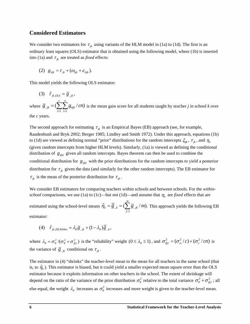
Considered Estimators
We consider two estimators for τ jk using variants of the HLM model in (1a) to (1d). The first is an ordinary least squares (OLS) estimator that is obtained using the following model, where (1b) is inserted into (1a) and τ jk are treated as fixed effects:
(2) gitjk = +τ jk (ω εtjk + itjk ).
This model yields the following OLS estimator:
(3) τ̂ jk O, .LS = g . jk , n
where g.. jk = (∑∑c
gitjk / cn) is the mean gain score for all students taught by teacher j in school k over t i= =1 1
the c years. The second approach for estimating τ jk is an Empirical Bayes (EB) approach (see, for example, Raudenbush and Bryk 2002; Berger 1985; Lindley and Smith 1972). Under this approach, equations (1b) to (1d) are viewed as defining normal “prior” distributions for the random intercepts ξtjk , τ jk , and ηk (given random intercepts from higher HLM levels). Similarly, (1a) is viewed as defining the conditional distribution of gijkt given all random intercepts. Bayes theorem can then be used to combine the
conditional distribution for gijkt with the prior distributions for the random intercepts to yield a posterior
distribution for τ jk given the data (and similarly for the other random intercepts). The EB estimator for
τ jk is the mean of the posterior distribution for τ jk . We consider EB estimators for comparing teachers within schools and between schools. For the within-school comparisons, we use (1a) to (1c)—but not (1d)—and assume that ηk are fixed effects that are
m
estimated using the school-level means η̂k k= =g... (∑g.. jk / m). This approach yields the following EB j=1
estimator: (4) τ̂ jk , ,EB Within = +λθ g.. jk (1−λθ )g...k , where λ σ= +2 2/( σ 2
θ θ θσ g |τ ) is the “reliability” weight (0 ≤ λθ ≤1) , and σ 2g |τ = +(σ 2
ω / c c) (σ 2ε / n) is
the variance of g.. jk conditional on τ jk . The estimator in (4) “shrinks” the teacher-level mean to the mean for all teachers in the same school (that is, to η̂k ). This estimator is biased, but it could yield a smaller expected mean square error than the OLS estimator because it exploits information on other teachers in the school. The extent of shrinkage will depend on the ratio of the variance of the prior distribution σ 2
θ relative to the total variance σ 2 2θ +σ g |τ ; all
else equal, the weight λθ increases as σ 2θ increases and more weight is given to the teacher-level mean.
6 Statistical Framework for the Teacher-Level Analysis
In practice, λθ will typically differ across teachers depending on available sample sizes, but we do not index λθ by j and k given the assumed balanced design. There are several EB estimators that could be used for the between-school comparisons. One estimator uses the four-level HLM model from above and is as follows: (5) τ λˆ jk ,EB,Between1 = +θ θg g.. jk (1−λ )[λψ ...k + (1−λψ )g.... ],
s
where g ˆ.... = =δ ( /∑ g...k s) is the grand district-level mean, λ σ= +2 2
ψ ψ /(σψ σ 2g |η ) is the between-
k=1
school reliability weight (0 ≤ ≤λψ 1) , and σ σ2 2g|η = +( / m c) (σ 2 / m)+ ( /σ 2
θ ω ε cnm) is the variance of
g...k conditional on ηk . This estimator shrinks the teacher-level mean toward the school-level mean, which, in turn, is shrunk toward the grand district-level mean (Raudenbush and Bryk 2002). This can be seen more clearly by rewriting (5) as follows: (5a) τ λˆ jk ,EB,Between1 = +θ ψ(g g.. jkλ ...k ) λψ (g...k − g.... )+ (1−λθ (1−λψ ))g..... Note that this approach could lead to result that a teacher with a higher value for g.. jk than another teacher is given a lower performance ranking because she teaches in a lower-performing school (which may be difficult to explain to educators). The second EB estimator that we consider does not adjust for performance differences across schools. It can be obtained from a three-level HLM model where (1d) is inserted into (1c). This estimator is as follows: (6) τ λˆ jk ,EB,Between2 = +τ τ'g g.. jk (1−λ ' ) .... , where λ σ 2 2 2
τ ' = +( )2 2θ ψσ /(σθ +σψ +σ g |τ ) is the between-school reliability weight (0 ≤ ≤λτ ' 1) . This
estimator directly shrinks the teacher-level mean to the grand district-level mean, and will ensure that teacher performance ratings will always be made based on g.. jk values, without regard to g...k values. For several reasons related to the clarity of presentation, we adopt the estimator in (6) rather than (5) for our analysis. First, for the system error rate analysis, we must calculate the variance of the EB estimator, which is the posterior distribution for τ jk given the data. This variance formula is very complex for the estimator in (5) (see Berger 1985), although it could be estimated through simulations using a Gibbs or related sampler (see, for example, Gelman et al. 1995; Gelman et al. 2007). The variance formula for the estimator in (6), however, is much simpler, as shown below. Second, it is more straightforward to use (6) rather than (5) to specify null hypotheses for comparing τ jk values for teachers across different schools so that the test statistics (z-scores) have zero expectations under the null hypotheses. This occurs because the expected value of the estimator in (5) is λθ θθ λjk + +( (1−λθ )λψ )ψ k +δ , whereas the expected value of the estimator in (6) is λτ ′ ( )θ ψjk + +k δ .
Thus, null hypotheses using (6) can focus on the equality of (θ jk k+ψ ) values across teachers, whereas
Statistical Framework for the Teacher-Level Analysis 7
null hypotheses using (5) must specify more complex conditions regarding the equality of θ jk and ψk values across teachers and schools. Schemes for Comparing Teacher Performance
In any performance measurement system, there must be a decision rule for classifying teachers as meriting or not meriting special treatment. One of the most prevalent value-added models applied in practice is the EVAAS model used by the Teacher Advancement Program (TAP; see National Institute for Excellence in Teaching 2009), which classifies each teacher into a performance category based on the t-statistic from testing the null hypothesis that the teacher’s performance is equal to average performance in a reference group (see Solmon et al. 2007; Springer et al. 2008). Thus, hypothesis testing is an integral part of the policy landscape in performance measurement, and forms the basis for our considered schemes for comparing teacher value-added estimates. This section discusses our considered schemes, in which we assume a classical hypothesis testing strategy for both the OLS and EB estimators. A comprehensive discussion of performance schemes is beyond the scope of this paper (see Podgursky and Springer 2007 for a detailed discussion). Rather, we outline several options that are used for the simulation analysis. Our results pertain to these options only. Scheme 1
The first considered design is a within-school scheme that aims to address the question, “Which teachers in a particular school performed particularly well or badly relative to all teachers in that school?” The
m
considered null hypothesis for this scheme is H :0 .τ jk −τ k = 0 , where τ.k = (∑τ jk / m) is the mean j=1
teacher effect in school k. Equivalently, the null hypothesis is that θ jk equals the mean θ jk value in school k. This testing approach will identify for special treatment teachers for whom the null hypothesis is rejected; the chances of identification will increase the further the teacher’s true performance is from her school’s mean. This scheme could be pertinent for school administrators who aim to identify exemplary or problem teachers in a particular school, without regard to the performance of teachers in other schools. Using the OLS approach and the estimator in (3), this null hypothesis can be tested using the z-score z g1,OLS = −[( .. jk g...k ) / V1,OLS ], where the variance V1,OLS is defined as follows:
σ σ2 2
ω ε m−1 (7) V1,OLS = +( )( ).
c cn m The first bracketed term in (7) is the variance of a teacher-level mean, and is the standard variance formula for a sample mean under a clustered design (see, for example, Cochran 1963; Murray 1998; Donner and Klar 2000). In our context, design effects arise because of the clustering of students within classrooms. The second bracketed term reflects the estimation error in the school-level mean and the covariance between the teacher- and school-level means. Importantly, for moderate m, the variance in (7) is driven primarily by the variance of the teacher-level mean (because the second bracketed term is close to 1). Thus, Scheme 1 has similar statistical properties to a more general scheme where statistical tests are conducted to compare a teacher’s performance
8 Statistical Framework for the Teacher-Level Analysis
relative to fixed threshold values that are assumed to be measured without error. Threshold values could be based, for example, on a percentile gain score in the state gain score distribution, or the average gain score such that a low-performing school or district would meet adequate yearly progress (AYP) benchmarks. These threshold values could effectively be assumed to have zero variance if they are based on very large samples or subjective assessment. Our results are also likely to be representative of schemes using fixed thresholds that do not involve hypothesis testing (although false positive and false negative error rate tradeoffs differ for these schemes and the ones that we consider). Using the EB approach and the estimator in (4), the null hypothesis for Scheme 1 can be tested with classical procedures using the z-score z g1,EB = −[ (λθ .. jk g...k ) / V1,EB )] , where V1,EB is an approximation
to the variance of the posterior distribution for τ jk given the data. This approximation, which assumes
that η̂k = g...k is estimated without error, is defined as follows:
m (8) V V1,EB = λθ 1,OLS ( ) = λ σ 2
m−1 θ τg | ,
where λθ is the within-school reliability weight defined above (see Gelman et al. 2009; Berger 1985). The variance of the EB estimator in (8) is smaller than the variance of the OLS estimator in (7) by a factor of λθm m/( −1) . Importantly, however, the z-score is smaller for the EB estimator by a factor of
λθ ( 1m− ) / m , suggesting that the OLS approach tends to reject the null hypotheses more often—and
thus has more statistical power than the EB approach. This occurs because as λθ decreases, the teacher-level means are shrunk toward their school-level means faster than the EB variances are shrunk toward zero. Gelman et al. (2009) argue that the smaller test statistics under the EB framework are appropriate for helping to reduce the multiple testing problem (see Schochet 2009). The multiple testing problem could plague the OLS approach because of the large number of comparisons that are likely to be made under a teacher performance measurement system, which could increase the chances of finding false positives. We do not consider multiple comparisons adjustments for the OLS estimator in this paper, which typically involve lowering significance levels with a resulting loss in statistical power. In some instances, school administrators—especially those in small schools—may want to compare the performance of two specific teachers (A and B) within the same school. In this design—referred to as Scheme 1a—the null hypothesis is H :0 τ Ak −τ Bk = 0 , and the z-score using the OLS approach is
z g1a O, LS = −[( ..Ak g..Bk ) / V1a O, LS ] , where the variance V1 ,a OLS is defined as follows:
2 2σ σ2 2
(9) V = +ω ε1 ,a OLS = 2σ 2
c cn g |τ .
For this scheme, the z-score under the EB approach is z g1a E, B = −[ (λθ ..Ak g..Bk ) / 2λ 2θ τσ g | ] .
Finally, we assume one-sided rather than two-sided tests, where the direction of the alternative hypothesis depends on the sign of the z-score. For instance, under Scheme 1, if the observed z-score is positive, then
Statistical Framework for the Teacher-Level Analysis 9
the alternative hypothesis is H :1 τ jk −τ .k 0 , > whereas if the observed z-score is negative, then the
alternative hypothesis is H :1 τ jk − <τ .k 0 . We adopt a one-sided testing approach, because it is likely that school administrators will want to gauge the performance of a teacher relative to others after examining the teacher’s performance measure. Scheme 2
The second considered design is a between-school scheme that aims to address the question, “Which teachers performed particularly well or badly relative to all teachers in the entire school district?” Under
s
this scenario, the considered null hypothesis is H :0 .τ jk −τ . = 0 , where τ τ.. = ( /∑ .k s) is the mean k=1
value of τ jk across all teachers in the district. Stated differently, the null hypothesis is that ( )θ jk k+ψ
equals the mean value of ( )θ jk k+ψ . Using the OLS approach, in which teacher and school effects remain fixed, the null hypothesis for Scheme 2 can be tested using the z-score z g2,OLS = −[( .. jk g.... ) / V2,OLS ] , where the variance V2,OLS is
defined as follows:
σ σ2 2 −1(10) V ω ε sm2,OLS = +( )( ).
c cn sm
The z-score using the EB approach is z g2,EB = −[ (λτ ' .. jk g.... )] / λ σ 2τ τ' g | .
Accounting for Tests From Multiple Subjects
The above analysis assumes that value-added estimates are obtained using gain scores from a single academic subject. However, value-added estimates for upper elementary school teachers are sometimes obtained using test score data from multiple subject areas. To account for these multiple tests in the variance calculations, we adopt the EVAAS approach where teacher effects are estimated separately for each subject area, and are then appropriately scaled and averaged to obtain aggregate value-added estimates that are used by policymakers. We assume that each subject test provides information on a teacher’s underlying τ jk value. Suppose that gain score data are available for d subject tests for each student in the classroom, so that nd test score observations are available for each classroom. These d test score observations are “clustered” within students, and now define Level 1 in the HLM model (where students are now Level 2, classrooms are Level 3, and so on). Standard methods on the variance of two-stage clustered designs (see, for example, Kish 1965) can then be used to show that the effective number of observations per classroom can be approximated as follows: (11) n neff ≈ +d /[1 ρd (d −1)],
10 Statistical Framework for the Teacher-Level Analysis
where ρd is the average pairwise correlation among the d tests. The denominator in (11) is the design effect, and will increase as the correlations between the subject tests increase. The design effect will equal d if ρd =1, in which case there are no precision gains from using the multiple tests. Conversely, the design effect will equal 1 if ρd = 0 , in which case the effective sample size is nd . To account for multiple tests in the above variance formulas, the effective class size, neff , can be used
rather than n . Realistic values for d and ρd are discussed below. Accounting for the Serial Correlation of Student Gain Scores Over Time
The benchmark HLM model uses only contemporaneous information on student test score gains to estimate the value-added of the students’ current teachers. However, some models such as EVAAS pool together gain scores from multiple grades for a given student, and information on gain scores from all available grades is used to estimate teachers’ value-added at a particular grade level. Because the student-level error term, ε itjk , may be serially correlated across grades, the gains achieved by a teacher’s current
students in other grades reduces uncertainty about the students’ current values of ε itjk and, hence, can improve the precision of the value-added estimates. Suppose that the HLM model in (1a) through (1d) is specified separately for two consecutive grades, and the two grade-specific models are estimated jointly as a system of seemingly unrelated regressions (SURs) using generalized least squares (GLS) (see, for example, the discussion of seemingly unrelated regressions in Amemiya 1985 and Appendix A). By comparing well-known variance formulas for the GLS estimator and the OLS estimator (Wooldridge 2002, Chapter 7), it can be shown that the variance of the SUR estimator is approximately the variance of the OLS estimator based on the effective number of observations per classroom, n neff 2 ≈ −/(1 ρ 2
t ,t−1) , where ρt t, 1− is the correlation of ε itjk across the two grades. Hence, the greater the absolute value of the serial correlation in the student-level error term, the greater the efficiency gains from exploiting serial correlation in estimation. In our sensitivity analysis, we present results using neff 2 rather than n, using empirical values of ρt t, 1− . As discussed below, empirical values of error correlations across non-consecutive grades are very small, so we do not consider the case of pooling more than two grades together. Measuring the Reliability of Performance Estimators
The variance formulas presented above have a direct relation to reliability (stability) measures that the previous literature has used to gauge the noisiness in value-added estimators (see, for example, McCaffrey et al. 2009). Reliability is the proportion of an estimator’s total variance across teachers that is attributable to persistent performance differences across teachers, and can be calculated as the correlation between a teacher’s value-added estimates for two non-overlapping time periods. In our notation, the reliability of the OLS estimator is λθ for the within-school analysis and λτ ′ for the between-school analysis. Clearly, reliability will increase as student sample sizes increase. Reliability in our context is parallel to the usual psychometric definition of reliability as the consistency of a set of measurements or of a measuring instrument, because both definitions aim to measure signal-to-noise ratios.
Statistical Framework for the Teacher-Level Analysis 11
In our view, reliability statistics are likely to carry little practical meaning for most stakeholders in a performance measurement system, unless they can be linked to a clear, direct measure of the accuracy with which the system can identify teachers who deserve special treatment. Thus, as discussed next, we use a direct approach to measure system misclassification rates. Nonetheless, we present reliability statistics for key simulation analyses. Calculating System Error Rates
In this section, we discuss our approach for defining system error rates for Schemes 1, 1a, and 2, and key issues that must be considered when applying these definitions. Defining System Error Rates
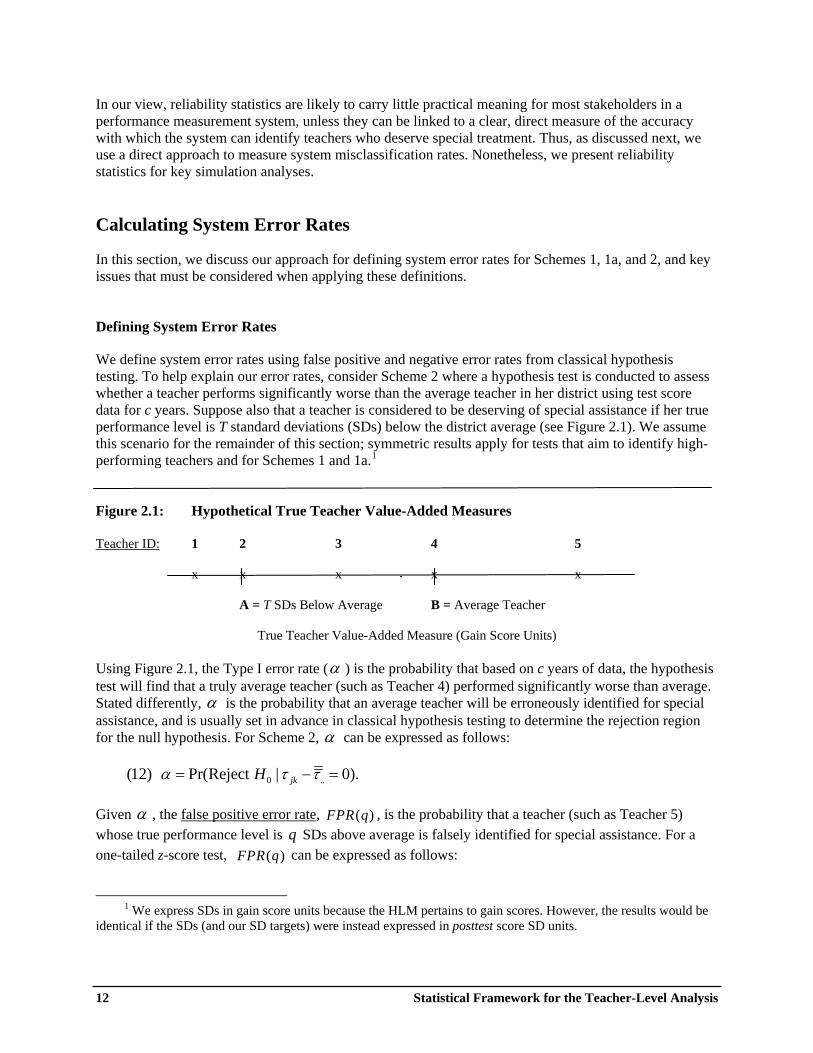
We define system error rates using false positive and negative error rates from classical hypothesis testing. To help explain our error rates, consider Scheme 2 where a hypothesis test is conducted to assess whether a teacher performs significantly worse than the average teacher in her district using test score data for c years. Suppose also that a teacher is considered to be deserving of special assistance if her true performance level is T standard deviations (SDs) below the district average (see Figure 2.1). We assume this scenario for the remainder of this section; symmetric results apply for tests that aim to identify high-performing teachers and for Schemes 1 and 1a.1 Figure 2.1: Hypothetical True Teacher Value-Added Measures Teacher ID: 1 2 3 4 5 x x x x x A = T SDs Below Average B = Average Teacher
True Teacher Value-Added Measure (Gain Score Units) Using Figure 2.1, the Type I error rate (α ) is the probability that based on c years of data, the hypothesis test will find that a truly average teacher (such as Teacher 4) performed significantly worse than average. Stated differently, α is the probability that an average teacher will be erroneously identified for special assistance, and is usually set in advance in classical hypothesis testing to determine the rejection region for the null hypothesis. For Scheme 2, α can be expressed as follows:
(12) α = −Pr(Reject H0 .|τ τjk . = 0). Given α , the false positive error rate, FPR( )q , is the probability that a teacher (such as Teacher 5) whose true performance level is q SDs above average is falsely identified for special assistance. For a one-tailed z-score test, FPR(q) can be expressed as follows:
1 We express SDs in gain score units because the HLM pertains to gain scores. However, the results would be identical if the SDs (and our SD targets) were instead expressed in posttest score SD units.
12 Statistical Framework for the Teacher-Level Analysis
(13) FPR(q) = −Pr(Reject H |τ τ = qσ ) =1−Φ [Φ−1 qσλ0 .jk . (1−α )+ ] for q ≥ 0,
V2
where σ 2 2= +(σ σ 2 2 2
ψ θ ω+σ +σε ) is the total variance of the student gain score, V2 is the variance of the
OLS or EB estimator for Scheme 2, λ equals 1 for the OLS estimator and λτ ' for the EB estimator, and Φ (.) is the normal distribution function. FPR( )q will decrease as the teacher’s true performance level increases beyond Point B in Figure 2.1 (that is, as q increases) and as the sample size increases. The Type I error rate equals FPR(0) . The overall false positive error rate for the population of average or better teachers can be obtained by calculating the expected value (weighted average) of population FPR( )q values:
(14) FPR _TOT = −∫ Pr(Reject H0 .|τ τjk . = q) f (q τ τ| jk − .. ≥ 0)∂q, q≥0
where f (.) is the density function of true teacher performance values for the considered population. Clearly, FPR _ TOT ≤ α . For the simulations, we assume that f (.) has a normal distribution with
variance V 2 2f =σθ /σ for the within school analysis and V ( 2 2 2
f = +σψ θσ σ) / for the between-school 2analysis, and estimate Vf using values that are discussed below. To calculate the integral in (14), we
used a simulation estimator where we (1) obtained 10,000 random draws for q from a truncated normal distribution, (2) calculated FPR( )q for each draw, and (3) averaged these 10,000 false positive error rates. Given α and the threshold value T , the false negative error rate is the probability that the hypothesis test will fail to identify teachers (such as Teachers 1 and 2 in Figure 2.1) whose true performance is at least T SDs below average. This error rate, FNR( )q , is the probability that a low-performing teacher will not be identified for special assistance, even though the teacher is deserving of such treatment. For a one-tailed z-score test, FNR( )q for Scheme 2 can be expressed as follows:
qσλ(15) FNR(q) = −Pr(Do Not Reject H0 .|τ τjk . = qσ ) = Φ [Φ−1(1−α )+ ] V 2
for q T≤ < 0 . This probability will decrease as the teacher’s true performance level moves further to the left of Point A in Figure 2.1. The Type II error rate, (1 − β ) , equals FNR ( )T , where β is the statistical power level. Note that T can be interpreted as the minimum difference in performance between a given teacher and the average that can be detected with a power level of β . Thus, our framework is parallel to the framework underlying minimum detectable effect sizes in impact evaluations (see, for example, Murray 1998; Bloom 2004; Schochet 2008).
2 In Scheme 1a, since the null hypothesis is that two given teachers do not differ in performance, f (.) is the density function of true differences in performance between two teachers, expressed in gain score standard deviations. The variance of these pairwise performance differences within schools is V 2 /2 2
f = σ θ σ .
Statistical Framework for the Teacher-Level Analysis 13
The overall false negative error rate for the population of low-performing teachers can be calculated as follows:
(16) FNR _TOT = −∫ FNR(q) f (q τ τ| jk .. ≤Tσ )∂q. q T≤ <0
Note that we do not include teachers in (16) whose performance values are between points A and B in Figure 2.1 (such as Teacher 3). This is because it is difficult to assess whether or not these teachers deserve special treatment and, in our simulations, we conduct calculations assuming different threshold values. We also define two additional aggregate error rates that have a Bayesian interpretation. First, for a given α , we define the population false discovery rate, FDR _ TOT , as the expected proportion of all teachers with significant test statistics who are false discoveries (that is, who are truly average or better).3 It is desirable that this error rate below to ensure that most teachers identified for special assistance are deserving of such treatment. Using Bayes rule, FDR _ TOT can be approximated as follows:
FPR _ *TOT .5(17) FDR _ TOT ≈ . ∫ Pr(Reject H 0 .|τ τjk − . = ∂qσ ) f (q q)
q
The denominator in (17) is the expected proportion of all teachers with significant test statistics, and includes teachers whose performance values are between points A and B in Figure 2.1. Second, for a given α and T , we define the false non-discovery rate, FNDR _ TOT , as the expected proportion of all teachers with insignificant test statistics who are truly low performers. This error rate can be approximated as follows:
FNR _ *TOT (1−Φ(| T |σ / V ) (18) FNDR _TOT ≈ f .
∫Pr(Do Not Reject H q0 .|τ τjk − . = ∂σ ) f (q) qq
Applying the System Error Rate Formulas
Several real-world issues must be considered to apply the error rate formulas for our simulations. A proper analysis must recognize that an assessment of the errors for a performance measurement system (and, hence, appropriate sample sizes) will depend on system goals and stakeholder perspectives. The remainder of this section discusses key issues and our approach for addressing them. Acceptable levels for false positive and false negative error rates. Tolerable error rates will likely depend on a number of factors. First, they are likely to depend on the nature of the system’s rewards and
3 The FDR was coined by Benjamini and Hochberg (1995) in the context of discussing methods to adjust for the multiple testing problem.
14 Statistical Framework for the Teacher-Level Analysis
Statistical Framework for the Teacher-Level Analysis 15
penalties. For instance, acceptable levels are likely to be lower if the system is to be used for making high-stakes decisions (such as promotions, merit pay decisions, firings, and identifying high-performing teachers who could be moved to low-performing schools) than for making less consequential decisions (such as identifying those in need of extra teacher professional development). Second, acceptable error rate levels are likely to differ by stakeholder (such as teachers, students, parents, school administrators, and policymakers) who may have different loss functions for weighing the various benefits and costs of correct and incorrect system classifications. For example, teachers may view false positives as more serious than false negatives for a system that is used to penalize teachers, because high false positive rates could impose undue psychic and economic costs on teachers who are falsely identified as low performers, thereby discouraging promising teachers from entering the teaching profession and reducing teacher morale. Teachers, however, may hold the opposite view for a system that is used to reward teachers. Parents, on the other hand, are likely to be primarily concerned that their children are taught by good teachers and, thus, may view false negatives as particularly problematic. As a final example, the loss function for school administrators is likely to be complex, because they must balance the loss functions of other stakeholders with competing interests, and must also consider their school report cards, the supply of qualified teachers in their local areas, and the positive and negative effects that a performance measurement system could have on the teacher supply. Because it is not possible to define universally acceptable levels for system error rates, we present error rates for different assumed numbers of years of available data, and are agnostic about what error rate levels are appropriate and whether false positives or false negatives are more problematic. The location of the threshold value for assessing system error rates. A critical issue for computing false negative rates is how to define high- and low-performing teachers. As is the case for determining tolerable error rates, the choice of threshold values will depend on stakeholder perspectives and system objectives. For example, parents may have a different view on what constitutes a low-performing teacher than school administrators or teachers. As discussed below, we define educationally meaningful threshold values using information on the natural progression of student test scores over time. Furthermore, we conduct the simulations using several threshold values to capture differences in stakeholder perspectives. The system error rates on which to focus. We focus on Type I and II error rates as well as the overall error rate measures discussed above, because these are likely to be of interest to a broad set of stakeholders. Type I and II error rates are likely to provide an upper bound on system error rates for individual teachers or schools. These rates may be applicable if the system is to be used for making high-stakes decisions and stakeholders view misclassification errors as highly consequential. The Type I error rate may be of particular interest to teachers or schools who believe that their performance is at least average (but who are not sure how much above average), because this rate is the maximum chance that such a teacher or school will be falsely identified for sanctions. Type I error rates may also be of interest to individuals who are considering entering the teaching profession and have no reason ex ante to believe that they are different from average. The Type II error rate may be of particular interest to administrators and parents who want a conservative estimate of the chances that a very low-performing teacher will be missed for special assistance and remain in the classroom without further intervention. We also present results using the overall error rate measures for those interested in aggregate misclassification rates for the full population of “good” and “poor” educators. Such interested parties might include designers of accountability systems whose focus is on the social equity of a performance measurement system. To these stakeholders, the issue that some “good” teachers and schools will have higher error rates than other “good” teachers and schools (and similarly for “poor” teachers and schools)
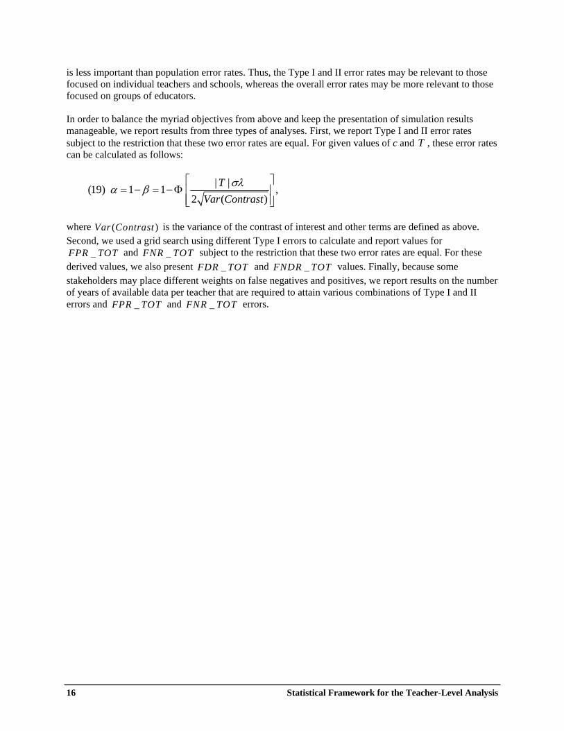
is less important than population error rates. Thus, the Type I and II error rates may be relevant to those focused on individual teachers and schools, whereas the overall error rates may be more relevant to those focused on groups of educators. In order to balance the myriad objectives from above and keep the presentation of simulation results manageable, we report results from three types of analyses. First, we report Type I and II error rates subject to the restriction that these two error rates are equal. For given values of c and T , these error rates can be calculated as follows:
⎡ ⎤| |T σλ(19) α β= −1 = −1 Φ ⎢ ⎥ , ⎣ ⎦⎢ ⎥2 (Var Contrast)
where Var (Contrast ) is the variance of the contrast of interest and other terms are defined as above. Second, we used a grid search using different Type I errors to calculate and report values for FPR _ TOT and FNR _ TOT subject to the restriction that these two error rates are equal. For these derived values, we also present FDR _ TOT and FNDR _ TOT values. Finally, because some stakeholders may place different weights on false negatives and positives, we report results on the number of years of available data per teacher that are required to attain various combinations of Type I and II errors and FPR _ TOT and FNR _ TOT errors.
16 Statistical Framework for the Teacher-Level Analysis
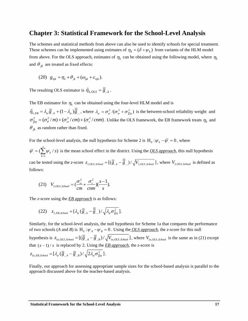
Chapter 3: Statistical Framework for the School-Level Analysis The schemes and statistical methods from above can also be used to identify schools for special treatment. These schemes can be implemented using estimates of ηk = (δ ψ+ k ) from variants of the HLM model from above. For the OLS approach, estimates of ηk can be obtained using the following model, where ηk
and θ jk are treated as fixed effects:
(20) gitjk = +ηk θ ωjk + ( tjk +ε itjk ).
The resulting OLS estimator is η̂k O, .LS = g ..k .
The EB estimator for ηk can be obtained using the four-level HLM model and is
η λˆ 2 2 2k E, B = +ψ ψg g...k (1−λ ) .... , where λ σψ ψ= +/(σψ σ g |η ) is the between-school reliability weight and
σ σ2 2g|η = +( /θ ωm c) (σ 2 / m)+ ( /σ 2
ε cnm) . Unlike the OLS framework, the EB framework treats ηk and
θ jk as random rather than fixed. For the school-level analysis, the null hypothesis for Scheme 2 is H :0 .ψ k −ψ = 0 , where
s
ψ . = ( /∑ψ k s) is the mean school effect in the district. Using the OLS approach, this null hypothesis k=1
can be tested using the z-score z g2,OLS ,School = −[( ...k g.... ) / V2,OLS ,School ] , where V2,OLS ,School is defined as
follows:
σ σ2 2ω ε s −1(21) V2,OLS ,School = +( )( ).
cm cnm s
The z-score using the EB approach is as follows:
(22) z g2,EB,School = −[λ λψ ψ( ...k g.... ) / σ 2g |η ].
Similarly, for the school-level analysis, the null hypothesis for Scheme 1a that compares the performance of two schools (A and B) is H :0 ψ A B− =ψ 0 . Using the OLS approach, the z-score for this null
hypothesis is z g1a,OLS ,School = −[( ...A g...B ) / V1a,OLS ,School ] , where V1 ,a OLS ,School is the same as in (21) except
that ( 1s − ) / s is replaced by 2. Using the EB approach, the z-score is
z g1a,EB,School = −[ (λ λ 2ψ ψ...A g...B ) / 2 σ g |η ] .
Finally, our approach for assessing appropriate sample sizes for the school-based analysis is parallel to the approach discussed above for the teacher-based analysis.
Statistical Framework for the School-Level Analysis 17

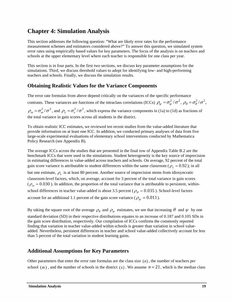
Chapter 4: Simulation Analysis This section addresses the following question: “What are likely error rates for the performance measurement schemes and estimators considered above?” To answer this question, we simulated system error rates using empirically based values for key parameters. The focus of the analysis is on teachers and schools at the upper elementary level where each teacher is responsible for one class per year. This section is in four parts. In the first two sections, we discuss key parameter assumptions for the simulations. Third, we discuss threshold values to adopt for identifying low- and high-performing teachers and schools. Finally, we discuss the simulation results. Obtaining Realistic Values for the Variance Components
The error rate formulas from above depend critically on the variances of the specific performance contrasts. These variances are functions of the intraclass correlations (ICCs) ρψ ψ=σ σ2 2/ , ρ 2 2
θ θ=σ σ/ ,
ρ =σ σ2 2ω ω / , and ρε ε=σ σ2 / 2 , which express the variance components in (1a) to (1d) as fractions of
the total variance in gain scores across all students in the district. To obtain realistic ICC estimates, we reviewed ten recent studies from the value-added literature that provide information on at least one ICC. In addition, we conducted primary analyses of data from five large-scale experimental evaluations of elementary school interventions conducted by Mathematica Policy Research (see Appendix B). The average ICCs across the studies that are presented in the final row of Appendix Table B.2 are the benchmark ICCs that were used in the simulations. Student heterogeneity is the key source of imprecision in estimating differences in value-added across teachers and schools. On average, 92 percent of the total gain score variance is attributable to student differences within the same classroom ( ρε = 0.92 ); in all but one estimate, ρε is at least 80 percent. Another source of imprecision stems from idiosyncratic classroom-level factors, which, on average, account for 3 percent of the total variance in gain scores ( ρω = 0.030 ). In addition, the proportion of the total variance that is attributable to persistent, within-school differences in teacher value-added is about 3.5 percent ( ρθ = 0.035 ). School-level factors
account for an additional 1.1 percent of the gain score variance ( ρψ = 0.011). By taking the square root of the average ρθ and ρψ estimates, we see that increasing θ and ψ by one standard deviation (SD) in their respective distributions equates to an increase of 0.187 and 0.105 SDs in the gain score distribution, respectively. Our compilation of ICCs confirms the commonly reported finding that variation in teacher value-added within schools is greater than variation in school value-added. Nevertheless, persistent differences in teacher and school value-added collectively account for less than 5 percent of the total variation in student learning gains. Additional Assumptions for Key Parameters
Other parameters that enter the error rate formulas are the class size ( )n , the number of teachers per school ( )m , and the number of schools in the district (s) . We assume n = 21, which is the median class
Simulation Analysis 19
size for self-contained classrooms in elementary schools according to our calculations from the 2003-04 School and Staffing Survey (SASS). The assumed value of m depends on the number of elementary grade levels that are likely to be included in a performance measurement scheme. Under No Child Left Behind (NCLB), state assessments must begin no later than third grade, so it is likely that longitudinal data systems will contain gain score data for fourth grade and beyond. However, some states and districts administer uniform assessments to their students in grades below third grade; for example, the California Standards Test (CST) begins in grade 2. Therefore, we make an optimistic assumption that each elementary school has three grade levels for which teacher value-added can be estimated, and that these three grades collectively have m =10 teachers (or an average of 3.3 teachers per grade). This assumption yields 70 students per grade level per school, which is approximately the median fourth grade enrollment of elementary schools in 2006-07 according to our calculations from the Common Core of Data. We assume multiple values of s because districts vary widely in size. In particular, we present results for s = 5 and s = 30 , which imply districtwide grade level enrollment in the 81st and 98th percentiles of district fourth grade enrollment in 2006-07. Our focus on the top quintile of district size stems from the fact that districts in this quintile educate more than 70 percent of the nation’s students. For our sensitivity analysis, we require values of d (the number of tests) and ρd (the average pairwise correlation between student gain scores from multiple tests). NCLB requires that elementary and middle school students be tested annually from grades 3 to 8 in reading and math, and tested at least once in science during grades 3 to 5 and 6 to 9. Districts must administer tests of English proficiency to all Limited English Proficient students, and sometimes administer their own tests in other subjects (such as social studies). It is likely, however, that most districts will consistently have available gain score data in at most 2 subject areas (reading and math); thus, we assume d = 2 for the sensitivity analysis. To obtain realistic values for ρd , we calculated correlations between math and reading fall-to-spring gain scores using the Mathematica data discussed in Appendix B. These correlations range from 0.2 to 0.4. Thus, for our analysis, we assume ρd = 0.3. Applying (11) with d = 2 , ρd = 0.3 , and n = 21 yields an
effective sample size, neff , equal to 32 students per classroom. Finally, the sensitivity analysis that exploits longitudinal student information from consecutive grades requires values of ρt t, 1− , the correlation of ε itjk across consecutive grades. Using data on the population of North Carolina’s students in third, fourth, and fifth grades, Rothstein (2010) finds that the correlation in gain score residuals between fourth and fifth grade is -0.38 in math and -0.37 in reading. Thus, our sensitivity analysis uses ρt t, 1− = −0.38 , implying an effective sample size of neff ,2 = 24.5 students per classroom. Importantly, Rothstein finds that the correlation between gain scores in grades three and five range from -0.02 to 0.02; thus, we ignore error correlations across non-consecutive grade levels. Identifying Threshold Values
A critical simulation issue for Schemes 1, 1a, and 2 is the threshold to adopt for defining meaningful performance differences between teachers or schools (that is, the value of T in Figure 2.1). Following the approach used elsewhere (Kane 2004; Schochet 2008; Bloom et al. 2008), we identify educationally meaningful thresholds using the natural progression of student test scores over time.
20 Simulation Analysis

Simulation Analysis 21
To implement this approach, we use estimates of average annual gain scores compiled by Bloom et al. (2008). For each of seven standardized test series, the authors use published achievement data for national samples of students who participated in the assessment’s norming study. Because these assessments use a “developmental” or “vertical” achievement scale, scale scores are comparable across grades within each assessment series. Thus, for each pair of consecutive grades, an estimate of the average annual gain score in SDs of test score levels can be estimated by (1) calculating the cross-sectional difference between average scale scores in the spring of the higher grade and the spring of the lower grade, and (2) dividing this difference by the within-grade SD of scale scores. Bloom et al. (2008) average these estimates across the seven test series for each grade-to-grade transition. To express the average gain score in terms of SDs of gain scores, we divide the final estimates of Bloom et al. (2008) by 0.696, the estimated ratio of the SD of test score gains to the SD of posttest scores from the Mathematica data discussed in Appendix B. Table 4.1 shows the resulting average annual gain scores expressed in gain score effect size units for each of three grade-to-grade transitions in the upper elementary grades. On average, annual growth in achievement per grade is 0.65 SDs of reading gains and 0.94 SDs of math gains. To help interpret these estimates, it is important to recognize these average gains reflect inputs to learning from both school-based settings and influences outside of school during a twelve-month period. In addition, a consistent pattern from prior studies is that average annual gains decrease considerably with grade level; hence, while our thresholds are selected in reference to typical learning growth in the upper elementary grades, different thresholds might be justifiable in lower or higher grades.
Table 4.1: Average Annual Gain Scores From Seven Nationally Standardized Tests
Grades Between Which Test Score Gains
Average Test Score Gain, in Standard Deviations of Gain Scores
are Calculated Reading Math
2 and 3 0.86 1.28
3 and 4 0.52 0.75
4 and 5 0.57 0.80
Average 0.65 0.94
Source: Authors’ calculations based on findings in Bloom et al. (2008).
Note: Figures for reading are based on the analysis of Bloom et al. (2008) for the following seven tests:
California Achievement Tests, Fifth Edition; Stanford Achievement Test Series, Ninth Edition; TerraNova Comprehensive Test of Basic Skills; Gates-MacGinitie Reading Tests; Metropolitan Achievement Tests, Eighth Edition; TerraNova, the Second Edition: California Achievement Tests; and the Stanford Achievement Test Series, Tenth Edition. Figures for math are based on all of the aforementioned tests except the Gates-MacGinitie. Calculations assume that one standard deviation of gain scores is equal to 0.696 standard deviations of test score levels, on the basis of data from the Mathematica evaluations listed in Table B.2.
Based on these estimates, we conduct our simulations for the teacher analyses using threshold values of 0.1, 0.2, and 0.3 SDs. A 0.2 value represents 31 percent of an average annual gain score in reading, or about 3.7 months of reading growth attained by a typical upper elementary student; in math, it represents 21 percent of an average annual gain score, or about 2.6 months of student learning. Importantly, these differences are large relative to the distribution of true teacher value-added: a performance difference of

Simulation Analysis 22
0.2 SDs in student gain scores is equivalent to the difference between a district’s 50th percentile teacher and its 82nd percentile teacher in terms of performance. In other words, a 0.2 SD threshold in Scheme 2 specifies that all teachers at or above the 82nd percentile of true performance deserve to be identified in a system for identifying high-performing teachers (or, symmetrically, that all teachers at or below the 18th percentile deserve to be identified in a system for identifying low-performing teachers). The other thresholds can be expressed in similar metrics: a 0.1 value represents 1.8 months of learning in reading, 1.3 months of learning in math, and the difference in performance between a district’s 50th and 68th percentile teachers, and a 0.3 value represents 5.5 months of learning in reading, 3.8 months of learning in math, and the difference in performance between a district’s 50th and 92nd percentile teachers.4 We use smaller threshold targets for the school analysis than for the teacher analysis. While thresholds retain the same “absolute” educational meaning regardless of whether teachers or schools are the units of comparison, we have seen that the variation in school value-added is smaller than the within-school variation in teacher value-added (that is, ρψ values tend to be smaller than ρθ values). Therefore, for school comparisons, we use thresholds that are half the size of those from the teacher comparisons; the resulting values of 0.05, 0.1, and 0.15 represent the differences between a district’s 50th percentile school and, respectively, its 68th percentile, 83rd percentile, and 92nd percentile schools. These performance differences amount, respectively, to 0.9, 1.8, and 2.8 months of learning in reading; in math, these performance differences amount, respectively, to 0.6, 1.3, and 1.9 months of learning. Simulation Results
Tables 4.2 through 4.9 provide the main findings from the simulation analysis for the considered estimators and performance measurement schemes. Tables 4.2 to 4.7 present results for the teacher-level analysis, while Tables 4.8 and 4.9 present results for the school-level analysis. The interpretation of the results in the tables will likely depend on the various considerations discussed above, such as acceptable system error rates, the relative weight that is placed on false negative and positive error rates, whether interest is on the individual-focused Type I and II error rates or on the group-focused overall error measures, and meaningful threshold values for defining low- and high-performing teachers and schools. How these factors are viewed may depend on the nature of the system rewards and sanctions as well as the stakeholder perspective. Accordingly, we report a range of estimates. Table 4.2 shows Type I and II error rates assuming that policymakers are indifferent between—and are thus willing to equalize—the two error rates. Table 4.4 displays parallel findings when FPR _ TOT and FNR _ TOT are restricted to be equal, and Table 4.6 displays associated false discovery and non-discovery rates. Table 4.3 shows reliability estimates for the OLS estimator. Because some readers may place different weights on false negatives and positives, Table 4.5 reports the number of years of data that are required to attain various combinations of system error rates. Table 4.7 shows how results change when key parameters are modified, and Tables 4.8 and 4.9 present key results for the school-level analysis.
4 These percentiles were calculated using results and assumptions from above that (1) teacher value-added
estimates are normally distributed; (2) one standard deviation of ( )θ +ψ is equivalent to 0.2145 standard deviations of gain scores (and thus that a 0.20 standard deviation increase in gain scores is equivalent to a 0.932 (0.20/0.2145) standard deviation increase in teacher value-added within the district); and (3) Φ (0.932) = 0.82. To express threshold values in terms of months of learning within each subject, threshold values in gain score effect size units were multiplied by 12 and divided by the average test score gain for the given subject (0.65 or 0.94) in Table 4.1.

Simulation Analysis 23
Table 4.2: Teacher-Level Analysis: Type I and II Error Rates that are Restricted to be Equal, by Threshold Value, Scheme, and Estimator
Threshold Value (Gain Score SDs from the Average)a
OLS Empirical Bayes (EB)
Number of Years of Available Data Per Teacher 0.1 0.2 0.3 0.1 0.2 0.3
Scheme 1: Compare a Teacher to the School Average (10 Teachers in the School)
1 0.42 0.35 0.28 0.46 0.42 0.38
3 0.37 0.25 0.16 0.40 0.31 0.23
5 0.33 0.19 0.10 0.36 0.25 0.15
10 0.27 0.11 0.03 0.30 0.15 0.06
Scheme 1a: Compare Two Teachers in the Same School
1 0.45 0.40 0.35 0.47 0.44 0.41
3 0.41 0.33 0.25 0.43 0.36 0.30
5 0.39 0.28 0.19 0.40 0.31 0.23
10 0.34 0.21 0.11 0.35 0.23 0.13
Scheme 2: Compare a Teacher to the District Average (50 Teachers in the District)
1 0.43 0.36 0.29 0.45 0.41 0.37
3 0.37 0.26 0.17 0.40 0.30 0.22
5 0.34 0.20 0.11 0.36 0.24 0.14
10 0.28 0.12 0.04 0.29 0.14 0.05
Scheme 2: Compare a Teacher to the District Average (300 Teachers in the District)
1 0.43 0.36 0.29 0.45 0.41 0.37
3 0.37 0.26 0.17 0.40 0.30 0.22
5 0.34 0.20 0.11 0.36 0.24 0.14
10 0.28 0.12 0.04 0.29 0.14 0.05
Note: See the text for formulas and assumptions. Calculations assume test score data from a single subject area.
aSee Figure 2.1 in the text for a depiction of these threshold values, which are measured in SDs of gain scores below or above the average true value-added measure in the appropriate population.
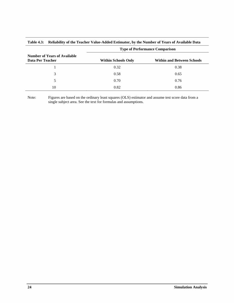
24 Simulation Analysis
Table 4.3: Reliability of the Teacher Value-Added Estimator, by the Number of Years of Available Data
Type of Performance Comparison
Number of Years of Available Data Per Teacher Within Schools Only Within and Between Schools
1 0.32 0.38
3 0.58 0.65
5 0.70 0.76
10 0.82 0.86 Note: Figures are based on the ordinary least squares (OLS) estimator and assume test score data from a
single subject area. See the text for formulas and assumptions.

Simulation Analysis 25
Table 4.4: Teacher-Level Analysis: Overall False Positive and Negative Error Rates that Are Restricted to be Equal
Threshold Value (Gain Score SDs from the Average)a
OLS Empirical Bayes (EB)
Number of Years of Available Data Per Teacher 0.1 0.2 0.3 0.1 0.2 0.3
Scheme 1: Compare a Teacher to the School Average (10 Teachers in the School)
1 0.26 0.21 0.17 0.36 0.33 0.30
3 0.16 0.10 0.06 0.21 0.16 0.12
5 0.11 0.06 0.03 0.15 0.10 0.06
10 0.06 0.02 0.01 0.08 0.04 0.01
Scheme 1a: Compare Two Teachers in the Same School
1 0.28 0.25 0.22 0.36 0.34 0.32
3 0.18 0.14 0.11 0.23 0.19 0.16
5 0.14 0.10 0.06 0.17 0.13 0.09
10 0.09 0.05 0.02 0.10 0.06 0.03
Scheme 2: Compare a Teacher to the District Average (50 Teachers in the District)
1 0.24 0.20 0.16 0.33 0.30 0.27
3 0.15 0.10 0.06 0.19 0.14 0.10
5 0.10 0.06 0.03 0.13 0.08 0.05
10 0.06 0.02 0.01 0.07 0.03 0.01
Scheme 2: Compare a Teacher to the District Average (300 Teachers in the District)
1 0.25 0.21 0.17 0.33 0.30 0.27
3 0.15 0.10 0.06 0.19 0.14 0.10
5 0.11 0.06 0.03 0.13 0.08 0.05
10 0.06 0.02 0.01 0.07 0.03 0.01
Note: See the text for formulas and assumptions. Calculations assume test score data from a single subject area.
aSee Figure 2.1 in the text for a depiction of these threshold values, which are measured in SDs of gain scores below or above the average true value-added measure in the appropriate population.
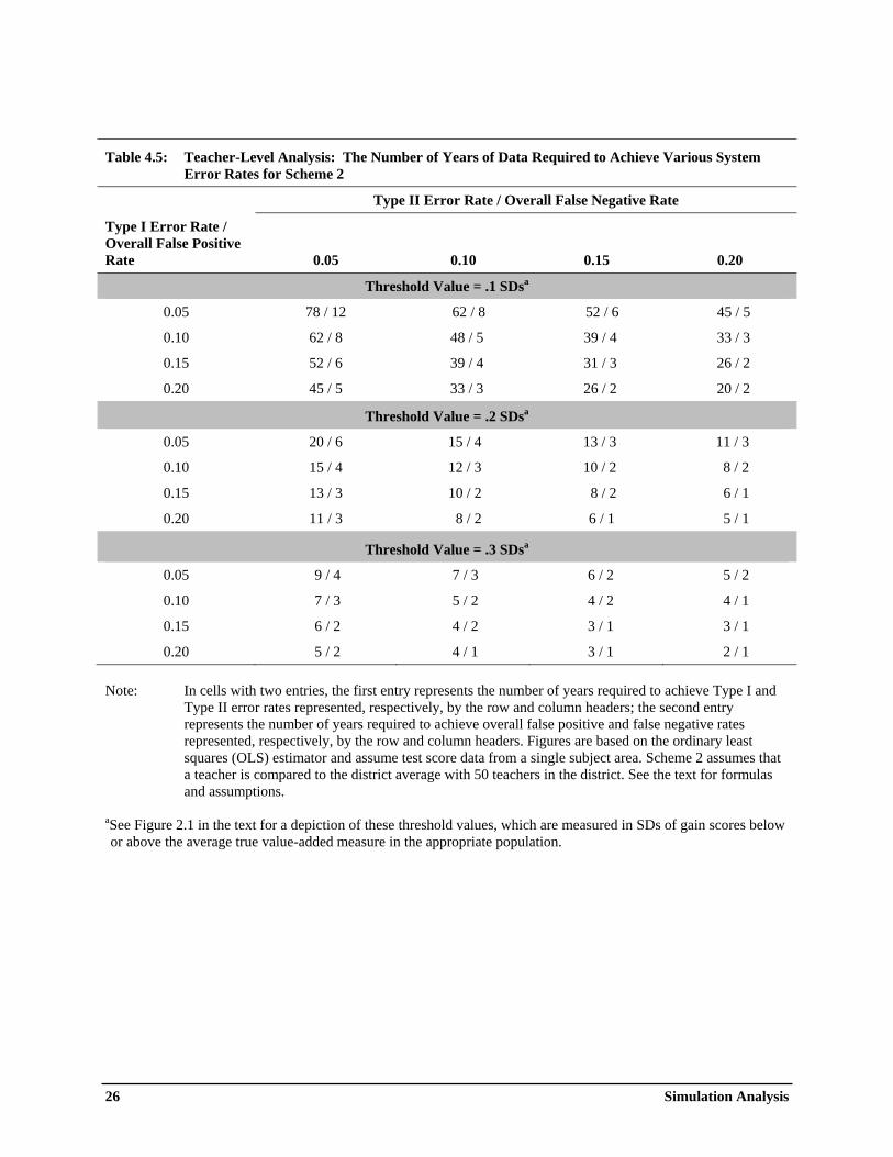
26 Simulation Analysis
Table 4.5: Teacher-Level Analysis: The Number of Years of Data Required to Achieve Various System Error Rates for Scheme 2
Type II Error Rate / Overall False Negative Rate
Type I Error Rate / Overall False Positive Rate 0.05 0.10 0.15 0.20
Threshold Value = .1 SDsa
0.05 78 / 12 62 / 8 52 / 6 45 / 5
0.10 62 / 8 48 / 5 39 / 4 33 / 3
0.15 52 / 6 39 / 4 31 / 3 26 / 2
0.20 45 / 5 33 / 3 26 / 2 20 / 2
Threshold Value = .2 SDsa
0.05 20 / 6 15 / 4 13 / 3 11 / 3
0.10 15 / 4 12 / 3 10 / 2 8 / 2
0.15 13 / 3 10 / 2 8 / 2 6 / 1
0.20 11 / 3 8 / 2 6 / 1 5 / 1
Threshold Value = .3 SDsa
0.05 9 / 4 7 / 3 6 / 2 5 / 2
0.10 7 / 3 5 / 2 4 / 2 4 / 1
0.15 6 / 2 4 / 2 3 / 1 3 / 1
0.20 5 / 2 4 / 1 3 / 1 2 / 1
Note: In cells with two entries, the first entry represents the number of years required to achieve Type I and Type II error rates represented, respectively, by the row and column headers; the second entry represents the number of years required to achieve overall false positive and false negative rates represented, respectively, by the row and column headers. Figures are based on the ordinary least squares (OLS) estimator and assume test score data from a single subject area. Scheme 2 assumes that a teacher is compared to the district average with 50 teachers in the district. See the text for formulas and assumptions.
aSee Figure 2.1 in the text for a depiction of these threshold values, which are measured in SDs of gain scores below or above the average true value-added measure in the appropriate population.

Simulation Analysis 27
Table 4.6: Teacher-Level Analysis: False Discovery and Non-Discovery Rates for Scheme 2 Using The Overall False Positive and Negative Error Rates in Table 4.4
Threshold Value (Gain Score SDs from the Average)a
0.1 0.2 0.3
Number of Years of Available Data Per Teacher
False Discovery
Rate
False Non-Discovery
Rate
False Discovery
Rate
False Non-Discovery
Rate
False Discovery
Rate
False Non-Discovery
Rate
1 0.27 0.14 0.25 0.06 0.23 0.02
3 0.17 0.08 0.13 0.03 0.10 0.01
5 0.12 0.06 0.08 0.02 0.05 0.00
10 0.07 0.03 0.03 0.01 0.01 0.00
Note: Figures are based on the OLS estimator and assume test score data from a single subject area. Scheme 2 assumes that a teacher is compared to the district average with 50 teachers in the district. See the text for formulas and assumptions.
aSee Figure 2.1 in the text for a depiction of these threshold values, which are measured in SDs of gain scores below or above the average true value-added measure in the appropriate population.

Table 4.7: Teacher-Level Analysis: Sensitivity of System Error Rates to Key ICC Assumptions and the Use of Multiple Tests
Type I = Type II Error Rate / False Negative = False Positive Error Rate for Scheme 2: Threshold=.2 SDsa
Number of Years of Number of Years of Number of Years of Data = 1 Data = 3 Data = 5
OLS EB OLS EB OLS EB Parameter Assumptions Estimator Estimator Estimator Estimator Estimator Estimator
Baseline Assumptions:
ρ = 0.92; ρ = 0.03;ε ω Single Subject Test 0.36 / 0.20 0.41 / 0.30 0.26 / 0.10 0.30 / 0.14 0.20 / 0.06 0.24 / 0.08
Sensitivity Analysis for ICC Parameters:
ρ = 0.80; ρ = 0.03 ε ω 0.35 / 0.12 0.37 / 0.15 0.25 / 0.05 0.27 / 0.06 0.19 / 0.03 0.20 / 0.03
ρ = 0.92; ρ = 0 ε ω 0.31 / 0.12 0.35 / 0.17 0.20 / 0.05 0.22 / 0.06 0.14 / 0.02 0.16 / 0.03
ρ = 0.87; ρ = 0.08 ε ω 0.39 / 0.25 0.44 / 0.36 0.31 / 0.14 0.36 / 0.21 0.26 / 0.10 0.30 / 0.14
Sensitivity Analysis for Multiple Subject Tests
d = 2 ;Tests ρ = 0.30d 0.34 / 0.18 0.39 / 0.26 0.24 / 0.08 0.27 / 0.11 0.18 / 0.04 0.21 / 0.06
Sensitivity Analysis for Longitudinal Gain Score
Data (Two Grades)
ρ 0.38, 1 = −t t− 0.35 / 0.19 0.40 / 0.28 0.25 / 0.09 0.29 / 0.13 0.19 / 0.05 0.23 / 0.07 Notes: In cells with two entries, the first entry represents the Type I and II error rates that are restricted to be
equal, and the second entry represents the overall false positive and false negative error rates that are restricted to be equal. For the sensitivity analysis for the ICC parameters, if changes in the values of the two indicated parameters do not offset each other, then the changes are assumed to be offset by changes in ρθ . Scheme 2 assumes that a teacher is compared to the district average with 50 teachers in the district.
ure 2.1 in the text for a depiction of this threshold value, which is measured in SDs of gain scores below or
the average true value-added measure in the appropriate population. aSee Figabove
28 Simulation Analysis
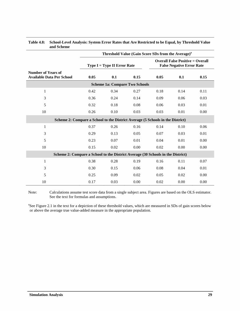
Simulation Analysis 29
Table 4.8: School-Level Analysis: System Error Rates that Are Restricted to be Equal, by Threshold Value and Scheme
Threshold Value (Gain Score SDs from the Average)a
Type I = Type II Error Rate Overall False Positive = Overall
False Negative Error Rate
Number of Years of Available Data Per School 0.05 0.1 0.15 0.05 0.1 0.15
Scheme 1a: Compare Two Schools
1 0.42 0.34 0.27 0.18 0.14 0.11
3 0.36 0.24 0.14 0.09 0.06 0.03
5 0.32 0.18 0.08 0.06 0.03 0.01
10 0.26 0.10 0.03 0.03 0.01 0.00
Scheme 2: Compare a School to the District Average (5 Schools in the District)
1 0.37 0.26 0.16 0.14 0.10 0.06
3 0.29 0.13 0.05 0.07 0.03 0.01
5 0.23 0.07 0.01 0.04 0.01 0.00
10 0.15 0.02 0.00 0.02 0.00 0.00
Scheme 2: Compare a School to the District Average (30 Schools in the District)
1 0.38 0.28 0.19 0.16 0.11 0.07
3 0.30 0.15 0.06 0.08 0.04 0.01
5 0.25 0.09 0.02 0.05 0.02 0.00
10 0.17 0.03 0.00 0.02 0.00 0.00
Note: Calculations assume test score data from a single subject area. Figures are based on the OLS estimator. See the text for formulas and assumptions.
aSee Figure 2.1 in the text for a depiction of these threshold values, which are measured in SDs of gain scores below or above the average true value-added measure in the appropriate population.

30 Simulation Analysis
Table 4.9: School-Level Analysis: The Number of Years of Data Required to Achieve Various System Error Rates for Scheme 2
Type II Error Rate / Overall False Negative Rate
Type I Error Rate / Overall False Positive Rate 0.05 0.10 0.15 0.20
Threshold Value = .05 SDsa
0.05 31 / 5 24 / 3 21 / 3 18 / 2
0.10 24 / 3 19 / 2 15 / 2 13 / 1
0.15 21 / 2 15 / 2 12 / 1 10 / 1
0.20 18 / 2 13 / 1 10 / 1 8 / 1
Threshold Value = .1 SDsa
0.05 8 / 2 6 / 2 5 / 2 4 / 1
0.10 6 / 2 5 / 1 4 / 1 3 / 1
0.15 5 / 1 4 / 1 3 / 1 3 / 1
0.20 4 / 1 3 / 1 3 / 1 2 / 1
Threshold Value = .15 SDsa
0.05 3 / 2 3 / 1 2 / 1 2 / 1
0.10 3 / 1 2 / 1 2 / 1 1 / 1
0.15 2 / 1 2 / 1 1 / 1 1 / 1
0.20 2 / 1 1 / 1 1 / 1 1 / 1
Note: In cells with two entries, the first entry represents the number of years required to achieve Type I and Type II error rates represented, respectively, by the row and column headers; the second entry represents the number of years required to achieve overall false positive and false negative rates represented, respectively, by the row and column headers. Figures are based on the ordinary least squares (OLS) estimator and assume test score data from a single subject area. Scheme 2 assumes that a school is compared to the district average with 30 schools in the district. See the text for formulas and assumptions.
aSee Figure 2.1 in the text for a depiction of these threshold values, which are measured in SDs of gain scores below or above the average true value-added measure in the appropriate population.
The key results can be summarized as follows: Finding 1: Using sample sizes typically available in practice, the considered performance measurement systems for teacher-level analyses will generally yield Type I and II error rates of at least 20 percent. Consider a system that aims to identify high-performing teachers in the upper elementary grades using sample sizes typically available in practice (1 to 5 years of data per teacher). Suppose also that policymakers find it acceptable to set α = 1− β and to set the threshold level for defining a high-performing teacher at 0.2 SDs above the average performance level (about 3 extra months of student learning per year in math and 4 months in reading). In this case, with c = 3 years of data, Scheme 2 (comparing a teacher to the district average) would yield a Type I or II error rate of 26 percent using the OLS estimator (Table 4.2). In other words, the system would miss for recognition more than one-fourth of truly high-performing teachers who are at the 82nd percentile of performance in their district, and would erroneously identify for recognition more than one-fourth of persistently average teachers. In this example, the Type I and II error rate for the OLS estimator is 25 percent for Scheme 1 (comparing a teacher to the school average) and 33 percent for Scheme 1a (comparing two teachers in the same school); the error rates are about 3 to 6 percentage points larger for the EB than OLS estimator (Table 4.2). Type I and II error rates would exceed one-third with only 1 year of data and would drop to one-fifth with 5 years of data (Table 4.2). The error rates would increase by about 10 percentage points using a threshold value of 0.1 SDs rather than 0.2 SDs, and would decrease by about 10 percentage points using a threshold value of 0.3 SDs (Table 4.2). Parallel results apply to systems that aim to identify below-average performers. To link these findings to typical analyses found in the literature, Table 4.3 shows the reliability of the OLS estimator for measuring teacher value-added. As discussed, reliability in our context is the proportion of an estimator’s total variance across teachers that is attributable to persistent performance differences across teachers. For c =1, about one-third to two-fifths of the total estimator variance across teachers is due to true, persistent performance differences. The remainder is due to student- and classroom-level variance factors. Reliability rises with c, consistent with the decrease in Type I and II error rates. For instance, reliability is about .60 for c = 3 and more than .70 for c = 5 . As discussed, we focus primarily on system error rates rather than reliability, because we believe that system error rates can be more easily interpreted by system stakeholders. An alternative approach for assessing system error rates is to calculate the number of years of data required to achieve various Type I and II error rates (Table 4.5). For a threshold value of 0.2 SDs, the OLS estimator would require about 11 years of data to ensure a Type I error rate of 5 percent and a Type II error rate of 20 percent (conventional levels used in hypothesis testing). Corresponding values are 45 years using a threshold value of 0.1 SDs and 5 years using a threshold value of 0.3 SDs. Importantly, the Type I error pertains to teachers of average performance, and the Type II error pertains to teachers whose performance is at the selected threshold value. As discussed, these error rates are likely to be of interest to those requiring upper bounds on system error rates for individual teachers. These rates, however, are likely to be larger than overall false positive and negative error rates that may be of interest to those requiring system misclassification rates for teachers as a group. To demonstrate this point, consider Scheme 2 for identifying high-performing teachers using c = 3 years of data. For this scenario, Figure 4.1 displays the false negative error rate by the distance between the teacher’s true performance level and the threshold value of 0.2 SDs above average (the solid line), and the estimated frequency of teachers at each performance level for the high-performing population (the dotted line).
Simulation Analysis 31

32 Simulation Analysis
False Negative Error Rates andandFigure 4.1: Population Frequencies for Scheme 2, by True Teacher Performance Level
Population Frequencies for Scheme 2, by True Teacher Performance Level
q = Distance of True Value Added Above T=.2 SDs FNR(q) calculations assume 0.26Note: α = and three years of available data. Frequency(q) is the normal density function at (q+T), that is proportionally scaled to satisfy the following restriction: the sum of the scaled density function across all input values from -5 to 5 in increments of 0.05 is set equal to1. The scaled density function is then multiplied by 10 to yield the values shown in the figure.
false ne
As can be seen in the figure, as true performance increases, the gative error rate decreases more sharply than the frequency distribution. Thus, small values of ( )FNR q beyond d value are assigned nontr s in the calculation of the overall false negative rate _
the thresholivial weight FNR TOT in (16). T
suggests that _his
FNR TOT is likely to be considerably smaller than the Type II error rate. A similar pattern holds for comparing the Type I error and the overall false positive rate (not shown). This analysis motivates our second key finding that is discussed next. Finding 2: Overall false negative and positive error rates for identifying low- and high-performing teachers are likely to be smaller than Type I and II error rates. Suppose that FNR _ TOT and FPR _ TOT are restricted to be equal for Scheme 2, and assume a threshold value of 0.2 SDs and c = 3. In this case, FNR _ TOT and FPR _ TOT equal 10 percent for the OLS estimator (Table 4.4), whereas α and (1 − β ) equal 26 percent when equated (Table 4.2). The corresponding error rates using the EB estimator are 14 and 30 percent, respectively. A similar pattern holds for the other schemes and threshold values. Consistent with these findings, fewer numbers of years of data are required to achieve various system error levels using the overall error rates than the Type I and II error rates (Table 4.5). For example, using a threshold value of 0.2 SDs, the OLS estimator would require about 3 years of data to ensure that FPR _ TOT = 0.05 and FNR _ 0TOT = .20 , compared to 11 years to ensure that α = 0.05 and (1− =β ) 0.20 . About 6 years of data would be required to achieve error rates of 5 percent for both FPR _ TOT and FNR _ TOT (Table 4.5).

Finally, Table 4.6 shows false discovery and non-discovery rates for Scheme 2 using the FPR _ TOT and FNR _ TOT values from Table 4.4. Assuming c = 3 and a threshold value of 0.2 SDs, the OLS estimator yields an FDR _ TOT value of 13 percent. This means that slightly more than one-eighth of teachers who are identified for special treatment are expected to be false discoveries; this error rate is larger than the corresponding 10 percent value for FPR _ TOT in Table 4.4. For this same scenario, FNDR _ TOT is 3 percent, which means that only a small percentage of all teachers with insignificant test statistics are expected to be misclassified. Finding 3: The simulation results for the teacher-level analysis are robust to alternative ICC assumptions, the use of two subject tests, and the use of two successive years of gain scores on each student. Our benchmark simulations were conducted using the average of the ICC values reported in Appendix Table B.2. However, because of the uncertainty in the ICC estimates and their critical role in the simulations, we examined the sensitivity of our main results by varying the key parameters ρω and ρε . As shown in Table 4.7, even if ρω and ρε were much lower than the benchmark values, the error rates would, in general, remain similar to those in Tables 4.2 and 4.4. Reducing ρε from 0.92 (the baseline assumption) to 0.80 (a value lower than all but one estimate in Appendix Table B.2), or reducing ρω to zero (which is equivalent to assuming that ω is a fixed effect specific to a teacher and year), leaves the Type I and II error rates at a minimum of 20 percent (assuming c = 3). The error rates for FPR _ TOT and FNR _ TOT , however, are somewhat more sensitive to lowering or raising the ICC values than the Type I and II errors. Allowing for multiple tests (for example, math and reading) instead of one test has little effect on the error rate estimates (Table 4.7). For instance, with c = 3, allowing for two tests decreases the Type I or II error rate from 0.26 to 0.24 and the overall false positive or negative rate from 0.10 to 0.08. Likewise, there are negligible reductions in error rates from using students’ gain scores in current and adjacent years—rather than in the current year only—as sources of information for estimating the performance of students’ current teachers (Table 4.7). For c = 3, both the Type I or II error rates and the overall false positive or negative error rates would decline by only 1 percentage point using the longitudinal approach. These analyses suggest that our benchmark findings, which are based on contemporaneous gain score data only, are likely to be applicable to value-added models such as EVAAS that exploit longitudinal gain score data on each student. Finding 4: Using the OLS estimator and comparable threshold values, the school-level analysis will yield error rates that are about 5 to 10 percentage points smaller than for the teacher-level analysis. With 3 years of data, the OLS estimator for Scheme 2 (comparing a school to the district average) would yield a Type I or II error rate of about 15 percent using a threshold value of 0.1 SDs—which is equivalent to setting the threshold for defining a high-performing school at the district’s 83rd percentile school (Table 4.8). The corresponding error rate for FPR _ TOT or FNR _ TOT is about 4 percent (Table 4.8). Under this scenario, about four years of data would be required to achieve conventional Type I and II error rates of α = 0.0 and 1 0− β = .20 , one year would be required to achieve values of FPR _ 0TOT = .05 and FNR _ 0TOT = .20 , and two years would be required to achieve values of 5 percent for both FPR _ TO and FNR _ TOT (Table 4.9). The school-level OLS analysis has more statistical power than the teacher-level OLS analysis, because school-level gain scores are estimated more precisely due to larger classroom and student sample sizes. Crucially, these precision gains occur because the variances of the OLS estimator are conditional on fixed
Simulation Analysis 33

values of θ jk and ψk . Statistical precision for the school-level analysis is much lower for the EB
estimator due to the variance contribution of θ jk (not shown).
34 Simulation Analysis

Summary and Conclusions 35
Chapter 5: Summary and Conclusions This paper has addressed likely error rates for measuring teacher and school performance in the upper elementary grades using student test score gain data and value-added models. This is a critical policyissue due to the increased interest in using value-added estimates to identify high- and low-performing instructional staff for special treatment, such as rewards and sanctions. Using rigorous statistical methods and realistic performance measurement schemes, the paper presents evidence that value-added efor teacher-level analyses are subject to a considerable degree of ra
stimates ndom error when based on the amount
d
than 1 nths
-
s for teacher-level estimates will be lower if the focus is on overall false positive ith
the r’s
ment ting
of data that are typically used in practice for estimation. Type I and II error rates for teacher-level analyses will be about 26 percent if three years of data are usefor estimation. This means that in a typical performance measurement system, more than 1 in 4 teacherswho are truly average in performance will be erroneously identified for special treatment, and morein 4 teachers who differ from average performance by 3 months of student learning in math or 4 moin reading will be overlooked. In addition, Type I and II error rates will likely decrease by only about onehalf (from 26 to 12 percent) using 10 years of data.
orresponding error rateCand negative error rates for the full populations of low- and high-performing teachers. For example, wthree years of data, misclassification rates will be about 10 percent. Our results are largely driven by findings from the literature and new analyses that more than 90 percent of the variation in student gain scores is due to the variation in student-level factors that are not undercontrol of the teacher. Thus, multiple years of performance data are required to reliably detect a teachetrue long-run performance signal from the student-level noise. In addition, our reported sample equirements likely understate those that would be required for an ongoing performance measurer
system, because our analysis ignores other realistic sources of variability, such as the nonrandom sorof students to classrooms and schools. Moreover, in practice, the multitude of comparisons made in a performance measurement system imply higher overall Type I error rates than those identified by our analyses, which ignore multiple comparisons issues. Our results strongly support the notion that policymakers must carefully consider system error rates in designing and implementing teacher performance measurement systems that are based on value-added models. Consideration of error rates is especially important when evaluating whether and how to use value-added estimates for making high-stakes decisions regarding teachers (such as tenure and firing decisions) (see Harris 2009). There are no universal definitions for tolerable system error rates and appropriate error rate measures. Rather, these decisions will likely depend on the nature of the system’s rewards and sanctions, and stakeholder perspectives on how to weigh the various benefits and costs of correct and incorrect system classifications. A performance measurement system at the school level will likely yield error rates that are about 5 to 10 percentage points lower than at the teacher level. This is because school-level mean gain scores can be estimated more precisely due to larger student sample sizes. Thus, current policy proposals to use value-added models for determining adequate yearly progress (AYP) and other school-level accountability ratings may hold promise from the perspective of statistical precision. An important caveat, however, is that biases may exist for estimating performance differences between schools, due, for instance, to nonrandom student sorting across schools. Our findings suggest that value-added estimates for teachers are likely to be noisy. However, it is important to emphasize that value-added measures have some key advantages over other alternative measures of teacher quality. Teacher value-added estimates in a given year are still fairly strong

36 Summary and Conclusions
predictors of subsequent-year academic outcomes in the teachers’ classes (Kane and Staiger 2008). In contrast, student achievement is only weakly associated with teachers’ credentials, education, experience, and other measurable characteristics (Hanushek and Rivkin 2006). Similarly, observational measures of classroom practices are often found to have little explanatory power in predicting student academic outcomes (see, for example, Constantine et al. 2009; Glazerman et al. 2009). While principals’ assessments of teacher effectiveness are reasonably accurate at identifying the best and worst teachers in a given school (Jacob and Lefgren 2008), their subjective nature leaves them more vulnerable to manipulation in a high-stakes setting than value-added measures. Our findings highlight the need to mitigate system error rates. Misclassification rates could be lower if value-added measures were carefully coordinated with other measures of teacher quality. For instance, value-added estimates may serve as an initial performance diagnostic that identifies a potential pool of teachers warranting special treatment. While our findings suggest that some teachers would be erroneously identified during this initial round, a subsequent round of more intensive performance measurement focused on this pool could further separate those who do and do not deserve special treatment. Indeed, Jacob and Lefgren (2008) find that value-added measures and principals’ assessments of teachers, in combination, are more strongly predictive of subsequent teacher effectiveness than each type of measure alone. System error rates may be reduced further through a number of implementation strategies that could improve the precision of the value-added estimates. For instance, developing tests with higher reliability could reduce the variation in student scores that is out of the teacher’s control. In addition, precision could be increased by implementing various types of teacher-student assignment mechanisms, such as the explicit balancing of student characteristics across classrooms and the assignment of each teacher to multiple classes per year. With these and other strategies, value-added measures could be a less error-prone component of the overall “toolbox” that policymakers use for performance measurement. Finally, it is important to recognize that our findings pertain to an important class of estimators and performance measurement schemes that conduct hypothesis tests based on value-added estimates used in isolation. However, spurred by large, recent infusions of funding from the federal government and private foundations, the development and application of teacher performance measures are ongoing and evolving, as districts have begun to explore new ways of combining value-added measures with other types of performance measures. Further research is warranted to determine the error rates generated by these and other schemes.

Appendix A: Comparing the HLM and EVAAS Models
The similarity of the variance estimates using the HLM and EVAAS models can be seen by comparing key features of the two models. For expositional purposes, we assume that both models aim to obtain teacher value-added estimates using students from a single large school who have available test score data from a single subject area. By inserting equations (1b) to (1d) into equation (1a) (and ignoring the k subscript since there is only one school), the HLM model can be expressed as follows:
(A1) gitj = +δ θ ωj + tj +ε itj . This model can be considered a repeated cross-section model of test score gains. The EVAAS model uses longitudinal data on students and directly models the growth in a student’s posttest scores over time as a function of the value-added of the student’s current and prior teachers. The model assumes that teacher effects persist unabated over time and are additive. This EVAAS layered model can be expressed as follows (see McCaffrey et al. 2004):
(A2) y I∑ ∑tit = +δ * *
t θ ε+ *c j=1 cj j it ,
where yit is the posttest score (not the gain score) for student i in year (grade) t, Icj is an indicator
variable that equals 1 if the student was taught by teacher j in year c and zero otherwise, θ *j is the teacher
effect for teacher j, ε*it is the student effect that can be correlated across years for the same student, and
δ *t is the mean posttest score in grade t. The EVAAS model does not include student- or classroom-level
covariates. The HLM model uses first differences of the test scores. The EVAAS model can also be expressed in terms of first differences as follows:
(A3) g yitj = −( it yi( 1t− −) ) = (δ δ* *t − t 1) +∑ j
I θ *ct j +uit ,
where uit = −(ε ε* *
it i( 1t− ) ) . This differencing removes teacher effects from prior grades as well as the part
of ε*it that remains constant over time (for example, a student’s innate ability).
Importantly, the model in (A3) reduces to the HLM model in (A1) if δ = −( )δ δ* * *
t t−1 , θ j = +θ ωj j. is
the value-added parameter of interest rather than θ j (so that teachers are fully responsible for their
classroom effects), and the uit s are uncorrelated across time for each student (see McCaffrey et al. 2004 for a similar point). The key issue then, is the extent to which the EVAAS model achieves precision gains by accounting for any (likely negative) dependence in the uit s for a student over time. This can be seen by comparing
Appendix A A-1

variances of estimated θ *j s from the EVAAS model that are obtained using two different approaches: (1)
an OLS approach that estimates (A1) or (A3) separately for two consecutive grades, and (2) a generalized least squares (GLS) approach that allows for cross-equation correlations among the uit s for each student. As discussed in Chapter 2, the variances of the GLS estimators are approximately equal to the variances of the OLS estimators based on an effective sample size of n n 2
eff 2 ≈ −/(1 ρt ,t−1) per classroom, where
ρt t, 1− is the correlation of uit across the two consecutive grades. Our sensitivity analysis in Chapter 4, which uses neff 2 in place of n, suggests that the HLM and EVAAS models are likely to yield value-added estimates that have similar variances.
A-2 Appendix A

Appendix B: Obtaining Realistic ICC Values
To obtain realistic ICC estimates, we reviewed ten recent studies from the value-added literature that provided information on at least one ICC. In addition, we conducted primary analyses of data from five large-scale experimental evaluations of elementary school interventions conducted by Mathematica Policy Research. Appendix Table B.1 displays the considered studies, the test score outcomes for each study, and the reported ICCs or combinations of ICCs. Because state assessments on which performance measures are likely to be based often begin in grade 3, we only reviewed studies that reported ICCs for at least one upper elementary grade.5 Furthermore, for studies that provided estimates separately by grade level or grade span, we focused on ICC estimates for the upper elementary grades. Most of the reviewed studies used student-level data from entire school districts or states across broad geographic areas. Some studies used longitudinal data, while others used gain score data from only one year—in which case it was not possible to obtain separate estimates for σ 2
ω
and σ 2θ . Importantly, for most studies, the ICCs in Appendix Table B.1 pertain to test scores measured in
levels rather than in gains.6 Thus, as discussed further below, we converted these ICCs into gain score units. To supplement the evidence from existing studies, we also analyzed student-level data from five Mathematica evaluations. Each evaluation included a geographically diverse but purposively selected set of schools that were willing to participate in the study. Two evaluations—the evaluations of Teach for America (Decker et al. 2004) and alternative teacher certification (Constantine et al. 2009)—are particularly suited for estimating ICCs, because students were randomly assigned to teachers within schools. The remaining three evaluations—covering early elementary math curricula (Agodini et al. 2009), education technology products (Dynarski et al. 2007), and supplemental reading comprehension interventions (James-Burdumy et al. 2009)—used schools’ usual assignment procedures for placing students into classrooms. The primary purpose of most of the reviewed studies was to obtain estimates of teacher value-added (that is, estimates of τ jk ). Thus, these studies typically reported only a subset of the ICCs required for our empirical analysis. However, additional ICCs could sometimes be calculated using other information reported by the studies. Furthermore, the combination of ICCs across studies formed a solid basis for obtaining realistic estimates for our simulations. The reviewed studies used two basic statistical approaches to calculate estimates of τ jk and associated ICCs (or combinations of ICCs). First, Nye et al. (2004) and McCaffrey et al. (2009) used standard maximum likelihood methods to directly estimate the variance components, an approach that we also used to analyze the data from the Mathematica evaluations. More commonly, the studies indirectly estimated variance components using estimates of τ jk , as discussed next.
5 See Aaronson et al. (2007) for a recent large-scale study of variation in teacher value-added within high
schools.
6 That is, many studies report a variance component of the gain score model in (1a) through (1d) as a ratio relative to the total variance in posttest scores. We will refer to these ratios as ICCs even if the numerators and denominators pertain to different units. In any case, all denominators are eventually converted to gain score units.
Appendix B B-1

B-2 Appendix B
Table B.1: Empirical Estimates of ICC Values Derivable Without Outside Information, by Study
Outcome Variable (Posttest or Gain Score)
Variance of Indicated Terms as a Ratio to Total Variance of Outcome Variable
Study Subject Grades ψ ψ θ+ θ θ ω+ ω Previous Studies Nye et al. (2004) Math 3 Posttest 0.048 0.123 Nye et al. (2004) Reading 3 Posttest 0.019 0.074 Rockoff (2004) Math K-6 Posttest 0.011 Rockoff (2004) Reading K-6 Posttest 0.009 Hanushek et al. (2005) Math 4-8 Gain Score 0.012 0.033 0.021 Rivkin et al. (2005) Math 4-7 Gain Score 0.013 Rivkin et al. (2005) Reading 4-7 Gain Score 0.009 Goldhaber and Hansen (2008) Math 5 Posttest 0.033 0.015 Goldhaber and Hansen (2008) Reading 5 Posttest 0.007 0.005 Kane et al. (2008) Math 4-5 Posttest 0.017 Kane et al. (2008) Reading 4-5 Posttest 0.010 Kane and Staiger (2008) Math 2-5 Posttest 0.005 0.053 0.048 0.032 Kane and Staiger (2008) English 2-5 Posttest 0.003 0.034 0.031 0.029 Koedel and Betts (2009) Math 4 Posttest 0.058 McCaffrey et al. (2009) Math 4-5 Posttest 0.022 0.018 Rothstein (2010) Math 5 Posttest 0.023 Rothstein (2010) Reading 5 Posttest 0.012 Data From Mathematica Evaluations Teach for America Reading 1-5 Gain Score 0.008 Teach for America Math 1-5 Gain Score 0.041 Teacher Certification Reading K-5 Gain Score 0.042 Teacher Certification Math K-5 Gain Score 0.019 Math Curricula Math 1 Gain Score 0.095 Education Technology: Grade 1 Reading 1 Gain Score 0.075 Education Technology: Grade 4 Reading 4 Gain Score 0.025 Reading Comprehension Reading 5 Gain Score 0.033
Source: Authors’ tabulations from the indicated studies and datasets.

Estimating σ 2 , ( )σ 2 2+σ , and σ 2
θ ψ θ ψ
Hanushek et al. (2005), Kane et al. (2008), and Kane and Staiger (2008) obtained estimates of ( )σ 2 2ψ +σθ
or σ 2θ using the relation that Cov( ,g. .tjk g t ' jk ) —the covariance between two separate estimates of τ jk
from different time periods—equals (σ 2 2ψ +σθ ) for models that do not include school effects, and σ 2
θ for models that do include school effects. Because Hanushek et al. (2005) and Kane and Staiger (2008) reported separate estimates for ( )σ 2 2
ψ +σθ and σ 2θ , we obtained estimates of σ 2
ψ through subtraction.
This “covariance” method was also used to obtain estimates of (σ 2 2ψ +σθ ) using reported results in
Goldhaber and Hansen (2008).
Estimating σ 2ω and ( )σ 2 2
θ +σω
Some studies reported sampling error variances of estimated τ jk values averaged across all teachers for a
single year (or by year). These error variances provided approximate annual estimates of ( /σ 2ε n) .
Because the total variance of τ̂ in a single year is Var( )g = +σ σ2 2 +σ 2.tjk ψ θ ω + (σ 2
jk ε / n) , estimates of
σ 2ω (or (σ 2 2
θ +σω ) ) can be obtained using reported estimates of Var( )g.tjk , ( /σ 2 2 2ε n) , σψ , and σθ . For
example, Goldhaber and Hansen (2008) and Kane and Staiger (2008) reported all four variance components needed to obtain σ 2
ω through subtraction. Koedel and Betts (2009) and Rothstein (2010) used
a similar approach to estimate (σ 2 2θ +σω ) using data from a single year.
Aggregating Estimates Across Studies For most studies, the ICCs in Appendix Table B.1 pertain to test scores measured in levels rather than in gains. Thus, in these cases, we converted the ICCs into gain score units by dividing the original ICCs by 0.484, our average estimate for the ratio of the variance of total gain scores to the variance of total posttest scores across all students in the Mathematica study samples. Appendix Table B.2 shows, for each study, ICC estimates for ρψ , ρθ , ρω , and
ρε = −(1 ρ ρψ θ− − ρω ) , where we imputed missing ICCs using information from other studies. The imputation procedure identified two sets of studies that contained information commonly missing from other studies: (1) studies that provided separate estimates of ρψ and ρθ (Hanushek et al. 2005; Kane and
Staiger 2008); and (2) studies in which an estimate of ρω was provided or could be directly inferred (Goldhaber and Hansen 2008; Kane and Staiger 2008; McCaffrey et al. 2009). From the first set of studies, we calculated the average value of ρ /( *
θ ρψ θ+ ρ ) , which we labeled R1 , and from the second
set of studies, we calculated the average value of ρ *ω /(ρ ρψ θ+ + ρω ) , which we labeled R2 . For each
study with missing ICCs, we then used R* , R*1 2 , or both to impute missing information. For example, if
ρω was the only missing ICC, we used R*2 for the imputations. Similarly, if ρψ was the only missing
ICC, we used R*1 for the imputations. This imputation procedure assumes that the ratios between ICCs
Appendix B B-3

are similar across studies, and it yields more robust results than if missing ICCs had been directly imputed using averages from other studies. The resulting average ICCs presented in the final row of Appendix Table B.2 are the benchmark ICCs that were used in the simulations.
Table B.2: Estimates of ICC Values Derived from Outside Information, by Study
Study-Reported Estimates and Imputation from
ICC Estimates for the HLM Model in (1a)-(1d) in Text
Study Subject
Schools (ρψ )
Teachers ( ρθ )
Classrooms ( ρω )
Students ( ρε )
Previous Studies Nye et al. (2004) Math 0.099 0.114 0.140 0.647 Nye et al. (2004) Reading 0.039 0.077 0.076 0.808 Rockoff et al. (2004) Math 0.005 0.019 0.016 0.960 Rockoff et al. (2004) Reading 0.004 0.016 0.013 0.967 Hanushek et al. (2005) Math 0.012 0.021 0.022 0.945 Rivkin et al. (2005) Math 0.003 0.013 0.010 0.974 Rivkin et al. (2005) Reading 0.002 0.009 0.007 0.982
Goldhaber and Hansen (2008) Math 0.013 0.056 0.030 0.900
Goldhaber and Hansen (2008) Reading 0.003 0.012 0.010 0.976 Kane et al. (2008) Math 0.007 0.028 0.023 0.942 Kane et al. (2008) Reading 0.004 0.017 0.014 0.966 Kane and Staiger (2008) Math 0.011 0.099 0.065 0.824 Kane and Staiger (2008) English 0.007 0.063 0.060 0.870 Koedel and Betts (2009) Math 0.015 0.066 0.053 0.866 McCaffrey et al. (2009) Math 0.009 0.037 0.037 0.918 Rothstein (2010) Math 0.006 0.026 0.021 0.948 Rothstein (2010) Reading 0.003 0.014 0.011 0.972
Data from Mathematica Evaluations Teach for America Reading 0.001 0.005 0.004 0.990 Teach for America Math 0.005 0.022 0.018 0.954 Teacher Certification Reading 0.005 0.023 0.019 0.953 Teacher Certification Math 0.002 0.010 0.009 0.979 Math Curricula Math 0.012 0.053 0.043 0.892 Education Technology: Grade 1 Reading 0.010 0.041 0.034 0.916 Education Technology: Grade 4 Reading 0.003 0.014 0.011 0.971 Reading Comprehension Reading 0.004 0.018 0.015 0.963
Average 0.011 0.035 0.030 0.923 Note: See the text for methods and assumptions.
B-4 Appendix B
References R-1
References
Aaronson, D., L. Barrow, and W. Sander (2007). Teachers and Student Achievement in the Chicago Public High Schools. Journal of Labor Economics, 25(1), 95-135.
Agodini, R., B. Harris, S. Atkins-Burnett, S. Heaviside, T. Novak, and R. Murphy (2009). Achievement
Effects of Four Early Elementary School Math Curricula: Findings from First Graders in 39 Schools (NCEE 2009-4052). Washington, DC: National Center for Education Evaluation and Regional Assistance, Institute of Education Sciences, U.S. Department of Education.
Amemiya, T. (1985). Advanced Econometrics. Cambridge, MA: Harvard University Press. Ballou, D. (2005). Value-Added Assessment: Lessons from Tennessee. In Value Added Models in
Education: Theory and Applications, edited by R. Lissetz. Maple Grove, MN: JAM Press. Ballou, D. (2009). Test Scaling and Value-Added Measurement. Education Finance and Policy 4(4), 351-
383. Ballou, D., W. Sanders, and P. Wright (2004). Controlling for Student Background in Value-Added
Assessment of Teachers. Journal of Educational and Behavioral Statistics, 29(1), 37-65. Benjamini, Y. and Y. Hochberg (1995). Controlling the False Discovery Rate. A New and Powerful
Approach to Multiple Testing. Journal of the Royal Statistical Society, Series B, 57, 1289-1300. Berger, J. (1985). Statistical Decision Theory and Bayesian Analysis. New York: Springer-Verlag. Bloom, H. (2004). Randomizing Groups to Evaluate Place-Based Programs. New York: MDRC. Bloom, H., C. Hill, A. Black, and M. Lipsey (2008). Performance Trajectories and Performance Gaps as
Achievement Effect-Size Benchmarks for Educational Interventions. New York: MDRC. Bloom, H., L. Richburg-Hayes, and A. Black (2007). Using Covariates to Improve Precision for Studies
that Randomize Schools to Evaluate Educational Interventions. Educational Evaluation and Policy Analysis, 29(1), 30-59.
Briggs, D. and J. Weeks (2009). The Sensitivity of Value-Added Modeling to the Creation of a Vertical
Score Scale. Education Finance and Policy 4(4), 384-414. Clotfelter, C., H. Ladd, and J. Vigdor (2006). Teacher-Student Matching and the Assessment of Teacher
Effectiveness. Journal of Human Resources, 41(4), 778-820. Cochran, W. (1963). Sampling Techniques. New York: John Wiley and Sons. Constantine, J., D. Player, T. Silva, K. Hallgren, M. Grider, M., and J. Deke (2009). An Evaluation of
Teachers Trained Through Different Routes to Certification, Final Report (NCEE 2009-4043). Washington, DC: National Center for Education Evaluation and Regional Assistance, Institute of Education Sciences, U.S. Department of Education.
Dallas Independent School District (2009). Performance Pay Programs. Retrieved October 13, 2009, from
http://www.dallasisd.org/performancepay/.
R-2 References
Decker, P., D. Mayer, and S. Glazerman (2004). The Effects of Teach For America on Students: Findings from a National Evaluation. Princeton, NJ: Mathematica Policy Research, Inc.
Donner, A. and N. Klar (2000). Design and Analysis of Cluster Randomization Trials in Health Research.
London: Arnold. Dynarski, M., R. Agodini, S. Heaviside, T. Novak, N. Carey, L. Campuzano, B. Means, R. Murphy, W.
Penuel, H. Javitz, D. Emery, and W. Sussex (2007). Effectiveness of Reading and Mathematics Software Products: Findings from the First Student Cohort. Washington, DC: U.S. Department of Education, Institute of Education Sciences.
Fischer, K. (2007). Dallas Schools’ Teacher Bonus Tied to Complex Ratings. The Dallas Morning News,
November 22. Retrieved October 13, 2009, from http://www.dallasnews.com/sharedcontent/dws/dn/education/stories/112307dnmetteachereval.2848ee7.html.
Gelman, A., J. B. Carlin, H. S. Stern, and D. Rubin (1995). Bayesian Data Analysis. London: Chapman
and Hall. Gelman, A., D. Dyk, Z. Huang, and W. J. Boscardin (2007). Transformed and Parameter-Expanded Gibbs
Samplers for Multilevel Linear and Generalized Linear Models. Department of Statistics Working Paper. New York: Columbia University.
Gelman, A. J. Hill, and M. Yajima (2009). Why We (Usually) Don’t Have to Worry About Multiple
Comparisons. Department of Statistics Working Paper. New York: Columbia University. Glazerman, S., S. Dolfin, A. Johnson, M. Bleeker, E. Isenberg, J. Lugo-Gil, M. Grider, and E. Briton
(2009). Impacts of Comprehensive Teacher Induction: Results from the First Year of a Randomized Controlled Study (NCEE 2009-4034). Washington, DC: National Center for Education Evaluation and Regional Assistance, Institute of Education Sciences, U.S. Department of Education.
Goldhaber, D. and M. Hansen (2008). Is it Just a Bad Class? Assessing the Stability of Measured Teacher
Performance. CRPE Working Paper 2008_5. Seattle, WA: Center on Reinventing Public Education. Gordon, R., T. Kane, and D. Staiger (2006). Identifying Effective Teachers Using Performance on the
Job. Hamilton Project Discussion Paper 2006-01. Washington, DC: The Brookings Institution. Hanushek, E., J. Kain, D. O’Brien, and S. Rivkin (2005). The Market for Teacher Quality. NBER
Working Paper 11154. Cambridge, MA: National Bureau of Economic Research. Hanushek, E. and S. Rivkin (2006). Teacher Quality. In Handbook of the Economics of Education, edited
by E. Hanushek and F. Welch. Amsterdam: North-Holland. Harris, D. (2009). Teacher Value-Added: Don’t End the Search Before It Starts. Journal of Policy
Analysis and Management, 28(4), 693-699. Harris, D. and T. Sass (2006). Value-Added Models and the Measurement of Teacher Quality. Working
Paper. Tallahassee, FL: Florida State University. Hedges, L. and E. Hedberg (2007). Intraclass Correlation Values for Planning Group-Randomized Trials
in Education. Educational Evaluation and Policy Analysis, 29(1), 60-87.

References R-3
Jackson, K. and E. Bruegmann (2009). Teaching Students and Teaching Each Other: The Importance of Peer Learning for Teachers. American Economic Journal: Applied Economics 1(4), 85-108.
Jacob, B. and L. Lefgren (2008). Can Principals Identify Effective Teachers? Evidence on Subjective
Performance Evaluation in Education. Journal of Labor Economics, 26(1), 101-136. Jacob, B., L. Lefgren, and D. Sims (2008). The Persistence of Teacher-Induced Learning Gains. NBER
Working Paper 14065. Cambridge, MA: National Bureau of Economic Research. James-Burdumy, S., W. Mansfield, J. Deke, N. Carey, J. Lugo-Gil, A. Hershey, A. Douglas, R. Gersten,
R. Newman-Gonchar, J. Dimino, and B. Faddis (2009). Effectiveness of Selected Supplemental Reading Comprehension Interventions: Impacts on a First Cohort of Fifth-Grade Students (NCEE 2009-4032). Washington, DC: National Center for Education Evaluation and Regional Assistance, Institute of Education Sciences, U.S. Department of Education.
Kane, T. (2004). The Impact of After-School Programs: Interpreting the Results of Four Recent
Evaluations. Working Paper. University of California, Los Angeles. Kane, T. and D. Staiger (2002a). The Promise and Pitfalls of Using Imprecise School Accountability
Measures. Journal of Economic Perspectives, 16(4), 91-114. Kane, T. and D. Staiger (2002b). Volatility in School Test Scores: Implications for Test-Based
Accountability Systems. In Brookings Papers on Education Policy: 2002, edited by D. Ravitch. Washington, DC: Brookings Institution Press.
Kane, T. and D. Staiger (2008). Estimating Teacher Impacts on Student Achievement: An Experimental
Evaluation. NBER Working Paper 14607. Cambridge, MA: National Bureau of Economic Research. Kane, T., J. Rockoff, and D. Staiger (2008). What Does Certification Tell Us About Teacher
Effectiveness? Evidence from New York City. Economics of Education Review, 27(6), 615-631. Kish, L. (1965). Survey Sampling. New York: John Wiley and Sons. Koedel, C. and J. Betts (2007). Re-Examining the Role of Teacher Quality in the Educational Production
Function. Working Paper. Columbia, MO: University of Missouri. Koedel, C. and J. Betts (2009). Does Student Sorting Invalidate Value-Added Models of Teacher
Effectiveness? An Extended Analysis of the Rothstein Critique. Working Paper. Columbia, MO: University of Missouri.
Lindley, D.V. and A.F.M. Smith (1972). Bayes Estimates for the Linear Model. Journal of the Royal
Statistics Society, Series B, 34, 1-41. McCaffrey, D., J.R. Lockwood, D. Koretz, and L. Hamilton (2003). Evaluating Value-Added Models for
Teacher Accountability. Santa Monica, CA: RAND. McCaffrey, D., J.R. Lockwood, D. Koretz, T. Louis, and L. Hamilton (2004). Models for Value-Added
Modeling of Teacher Effects. Journal of Educational and Behavioral Statistics, 29(1), 67-101. McCaffrey, D., T. Sass, J.R. Lockwood, and K. Mihaly (2009). The Intertemporal Stability of Teacher
Effects. Education Finance and Policy 4(4), 572-606.

R-4 References
Murray, D. (1998). Design and Analysis of Group-Randomized Trials. Oxford: Oxford University Press. National Institute for Excellence in Teaching (2009). TAP: The System for Teacher and Student
Advancement. Retrieved from http://www.tapsystem.org/ on October 13, 2009. Nye, B., S. Konstantopoulos, and L. Hedges (2004). How Large are Teacher Effects? Educational
Evaluation and Policy Analysis, 26(3), 237-257. Podgursky, M. and M. Springer (2007). Teacher Performance Pay: A Review. Journal of Policy Analysis
and Management, 26(4), 909-949. Raudenbush, S. and A. Bryk (2002). Hierarchical Linear Models: Applications and Data Analysis
Methods, second edition. Thousand Oaks, CA: Sage Publications, Inc. Rivkin, S., E. Hanushek, and J. Kain (2005). Teachers, Schools, and Academic Achievement.
Econometrica, 73(2), 417-458. Rockoff, J. (2004). The Impact of Individual Teachers on Student Achievement: Evidence from Panel
Data. American Economic Review (AEA Papers and Proceedings), 94(2), 247-252. Rockoff, J., B. Jacob, T. Kane, and D. Staiger (2008). Can You Recognize an Effective Teacher When
You Recruit One? NBER Working Paper 14485. Cambridge, MA: National Bureau of Economic Research.
Rogosa, D. (2005). Statistical Misunderstandings of the Properties of School Scores and School
Accountability. Yearbook of the National Society for the Study of Education, 104(2), 147-174. Rothstein, J. (2010). Teacher Quality in Educational Production: Tracking, Decay, and Student
Achievement. Quarterly Journal of Economics 125(1), 175-214. Sanders, W. L., Saxton, A. M., and Horn, S. P. (1997). The Tennessee Value-Added Assessment System:
A Quantitative, Outcome-Based Approach to Educational Assessment. In J. Millman (ed.), Grading Teachers, Grading Schools: Is Student Achievement a Valid Evaluation Measure?. Thousand Oaks, CA: Corwin Press, 137-162.
Schochet, P. Z. (2008). Statistical Power for Random Assignment Evaluations of Education Programs.
Journal of Educational and Behavioral Statistics, 33(1), 62-87. Schochet, P. Z. (2009). An Approach for Addressing the Multiple Testing Problem in Social Policy
Evaluations. Evaluation Review, forthcoming. Solmon, L., J.T. White, D. Cohen, and D. Woo (2007). The Effectiveness of the Teacher Advancement
Program. Santa Monica, CA: National Institute for Excellence in Teaching. Springer, M., D. Ballou, and A. Peng (2008). Impact of the Teacher Advancement Program on Student
Test Score Gains: Findings from an Independent Appraisal. Working Paper 2008-19. Nashville, TN: National Center on Performance Incentives.
Todd, P. and K. Wolpin (2003). On the Specification and Estimation of the Production Function for
Cognitive Achievement. The Economic Journal, 113, F3-F33.

References R-5
U.S. Department of Education (2009). Race to the Top Fund – Executive Summary: Notice of Proposed Priorities, Requirements, Definitions, and Selection Criteria. Washington, DC: U.S. Department of Education.
Wooldridge, J. (2002). Econometric Analysis of Cross Section and Panel Data. Cambridge, MA: MIT
Press.


