Shifting Optimization of Face Dog Clutches in Heavy Duty Automated Mechanical Transmissions Ph.D. Thesis GERGELY BÓKA Supervisor: János Márialigeti External supervisor: László Palkovics Vehicles and Mobile Machines Ph.D. School Budapest University of Technology and Economics Faculty of Transportation Engineering Department of Vehicle Parts and Drives Budapest, Hungary 2011
Transcript
Shifting Optimization of Face Dog Clutches in Heavy
Duty Automated Mechanical Transmissions
Ph.D. Thesis
GERGELY BÓKA
Supervisor: János Márialigeti
External supervisor: László Palkovics
Vehicles and Mobile Machines Ph.D. School
Budapest University of Technology and Economics
Faculty of Transportation Engineering
Department of Vehicle Parts and Drives
Budapest, Hungary
2011
2
Foreword
This Thesis summarizes my research work completed as a Ph.D. student at the Department of
Vehicle Parts and Drives during my studies in the Vehicles and Mobile Machines Ph.D. School of the
Budapest University of Technology and Economics. The scientific part was mostly, the
measurements were entirely carried out in the Knorr-Bremse Research and Development Centre.
The essence of this work has already been published in pieces in different journals and conference
proceedings, as listed in Section 5. The core of this Thesis is the natural chain of those publications,
however, based on a unified and simplified nomenclature and completed with an extended
introductory part on the state of the art.
However, without the help, professional advices or simple, encouraging kind words of the
colleagues at both institutes, all my efforts would have remained pointless.
In particular, in the team of the Department of Vehicle Parts and Drives, I would like to express my
honest gratitude to Mr. András Eleőd, the head of the Department, who supported me in all possible
ways in the Ph.D. school, to my supervisor, Mr. János Márialigeti, for sharing his knowledge and
experiences with me and to Mr. László Lovas, for the first steps in the scientific world.
In the team of the Knorr-Bremse Research and Development Centre, I am highly grateful to my
external supervisor, Mr. László Palkovics, the head of the institute, for making this research work
possible, to Mr. Huba Németh, for the guiding and inspiration and last but not least to Mr. Balázs
Trencséni for supporting me in the everyday work and for the common brain storming, where the
core ideas of this Thesis were born.
The road to this work also required many personal sacrifices. I will be forever thankful to my family
and friends who still stayed with me all the time.
The undersigned, Gergely Bóka declares that this Ph.D. thesis has been prepared by him using only
the indicated sources. All parts that have been taken over literally or by content are cited
unambiguously.
Alulírott Bóka Gergely kijelentem, hogy ezt a doktori értekezést magam készítettem és abban csak a
megadott forrásokat használtam fel. Minden olyan részt, amelyet szó szerint, vagy azonos
tartalomban, de átfogalmazva más forrásból átvettem, egyértelműen, a forrás megadásával
megjelöltem.
München, 2011.11.03.
………………………………………………
3
Abstract
This Thesis deals with the optimisation of the engagement of face dog clutches in the constant mesh
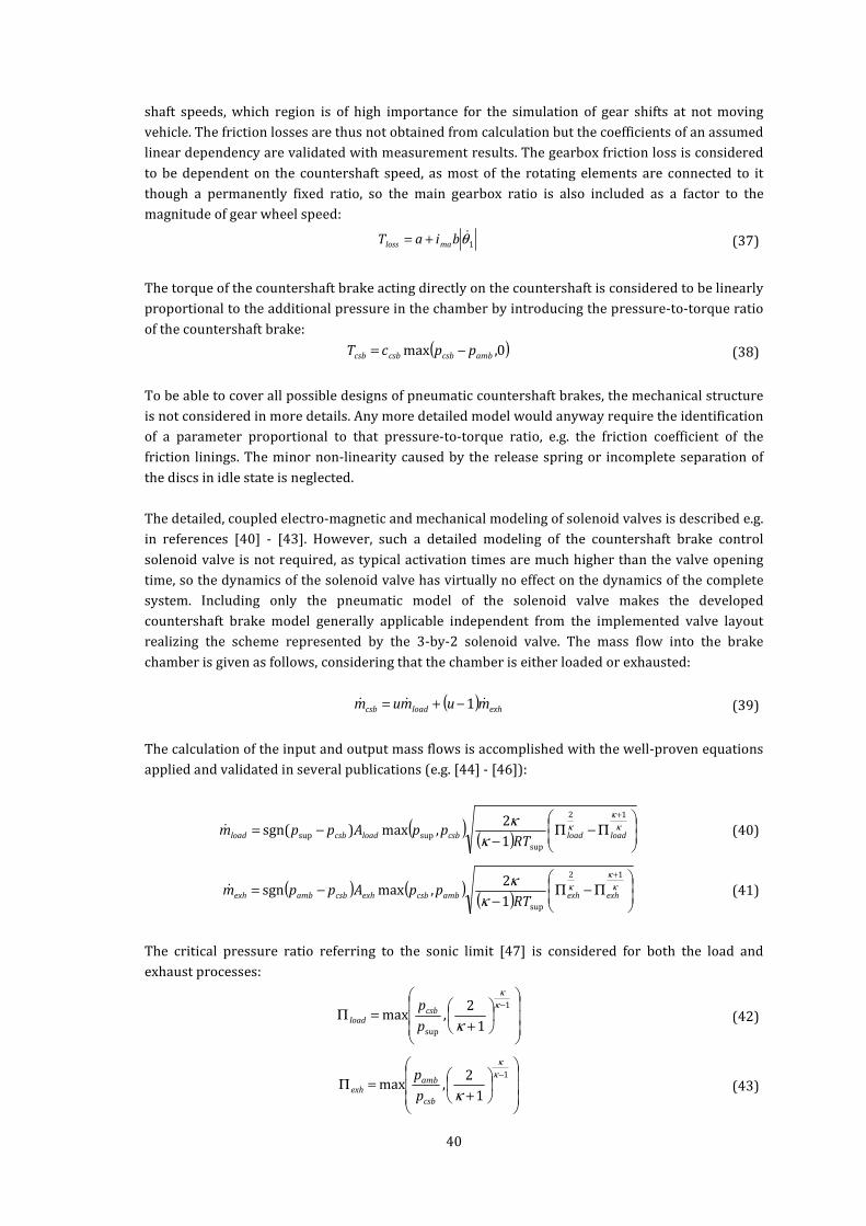
gearbox of Automated Mechanical Transmissions of modern heavy duty commercial vehicles. To
increase the torque capacity and reduce the mechanical complexity of the gearbox, some of the
engaging devices are simple dog clutches without of synchromesh, synchronized at upshifts and at
gear shifts from neutral by means of a countershaft brake actuated in a precisely metered way in
order to quickly enter the narrow zone of suitable engagement conditions. The quality of the dog
shifting has a determining factor in the harshness of the whole gearshift process, and therefore
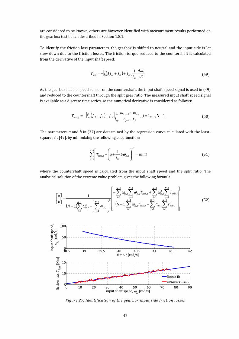
needs a continuous improvement to meet the ever increasing customer demands.
The preceding countershaft brake actuation causes special conditions for the engagement which
are merely different from all other automotive applications of dog clutches. The interactions
leading to the unwanted permanent tooth-on-tooth situations resulting in an unsuccessful
engagement attempt are only possible to be explained with an integrated approach regarding the
so far separately treated mechanical sub-systems of the dog clutch and the countershaft brake. The
understanding of the special characteristics of dog clutch engagement in heavy duty automated
gearboxes which is practically uncovered in scientific publications enables the reduction of the
mismatch speed at the engagement and this way the reduction of the torsional vibrations and
gearshift noise.
The Thesis is divided into 5 main parts. Chapter 1 presents an overview of the state of the art of the
relevant transmission control related topics, such as the mechanical layout and gearshift process of
heavy duty Automated Mechanical Transmissions, design and actuation principles of countershaft
brakes, the characteristics of face dog clutches and finally, the measuring systems used for
collecting measurement data.
The engaging capability of face clutches and the influencing factors, in particular the pressure in the
countershaft brake chamber are investigated in Chapter 2. Two mechanical models – a basic and a
more detailed one – are developed both utilizing a probability approach to describe the occurrence
of unsuccessful engagements due to permanent tooth-on-tooth situations. The unknown
parameters are identified and the models are validated with test bench measurement results.
Based on the results of Chapter 2, the optimal engaging conditions referred as the synchronized
state of face dog clutches at gear shifts with countershaft brake actuation are highlighted in Chapter
3. The new, enhanced approach is implemented in a synchronizing algorithm in order to prove the
feasibility of the proposed new definition of the synchronized state and is evaluated with results of
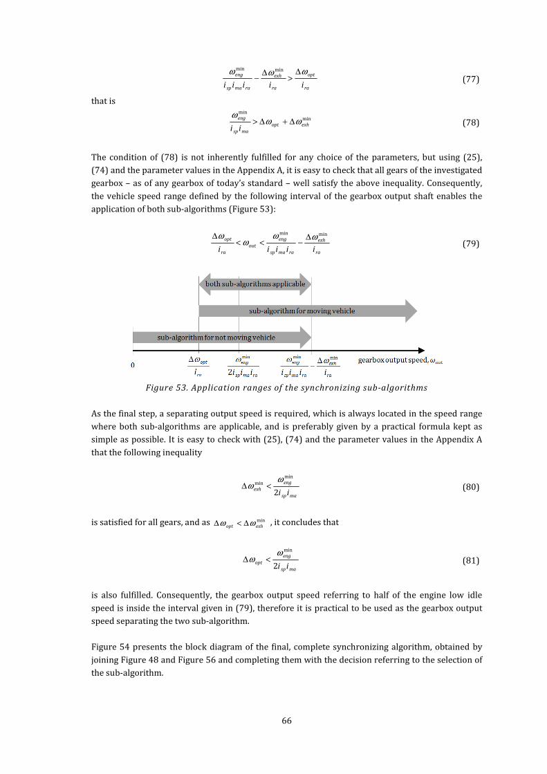
bench and vehicle tests.
The results of this work are summarized in forms of theses along with the list of publications
published during the research work in Chapters 4 and 5.
And finally, after the list of references, Appendices A and B include all the parameter values,
MATLAB/Simulink models and scripts related to the simulation and visualization of the new results
of this Thesis, making all achievements – excluding the confidential measurement data and the
exact implementation of the synchronizing algorithm – completely reproducible for the Reader.
4
Auszug
In dieser Dissertation handelt es sich um die Optimierung des Schaltvorganges der
Klauenkupplungen in automatisierten schwer-LKW Getrieben. Um die Tragfähigkeit zu steigern
und die mechanische Komplexität des Getriebes zu reduzieren, sind einige Schaltkupplungen keine
Selbstsynchronisierenden, sondern einfache Klauenkupplungen, die für Hochschaltungen und
Schaltungen von Neutralgang durch eine Vorgelegewellebremse synchronisiert werden. Die präzis
angesteuerte Betätigung dieser Bremse ermöglicht, dass die geeigneten Schaltbedingungen schnell
erreicht werden. Die Rauigkeit des gesamten Schaltvorganges ist durch die Qualität der
Klauenschaltungen stark beeinflusst, deshalb benötigt sie eine kontinuierliche Verbesserung um die
ständig steigenden Kundenanforderungen nach wie vor treffen zu können.
Die vorangehende Betätigung der Vorgelegewellebremse verursacht solche speziellen Zustände für
die Schaltungen, die sich von anderen fahrzeugbedingten Applikationen grundsätzlich
unterscheiden. Die Wechselwirkungen, die zu Fehlschaltungen mit permanenter Zahn-auf-Zahn
Auflage führen können, sind nur durch die integrierte Modellierung von der bisher getrennt
betrachteten Klauenkupplung und Vorgelegewellebremse zu erklären. Die Erfassung der in
wissenschaftlichen Publikationen praktisch unbedeckten Sonderzustände der Klauenschaltungen
ermöglicht die Reduzierung des Geschwindigkeitsversatzes und in Folge, die Verringerung der
Schwenkungen und Schaltgeräusch.
Diese Dissertation verfügt über 5 Haupteile. Kapitel 1 präsentiert eine Durschicht des Standes der
Technik bezüglich der relevanten antriebstrangbezogenen Themen, wie der Aufbau und
Schaltvorgang automatisierter schwer-LKW Getriebe, Konstruktion und Betätigungsprinzip von
Vorgelegewellebremsen, Verhalten von Klauenkupplungen und schließlich, die Messsyteme, die für
die Erstellung der Messergebnisse in dieser Dissertation verwendet wurden.
Die Schaltfähigkeit von Klauenkupplungen und die Einflussfaktoren – besonders der Druck in der
Kammer der Vorgelegewellebremse – sind in Kapitel 2 untersucht. Es sind 2 Berechnungsmodelle
entwickelt worden, um die Auftrittswahrscheinlichkeit der wegen permanenten Zahn-auf-Zahn
Auflagen erfolglosen Schaltungen zu berechnen. Die Identifikation der unbekannten Parameter und
die Validierung der Berechnungsmodele erfolgen durch Prüfstandsmessungen.
Aufgrund der Ergebnisse von Kapitel 2, die optimale Schaltbedingungen sind in Kapitel 3 erläutert,
erwähnt als der synchronisierte Stand der Klauenkupplung für Gangwechsel mit Betätigung der
Vorgelegewellebremse. Um die Machbarkeit zu überprüfen ist ein Synchronisierungsalgorithmus
mit der neuen, verfeinerten Bestimmung entwickelt und mit Prüfstands- bzw. Fahrzeugmessungen
evaluiert worden.
In den Kapiteln 4 und 5 sind die Ergebnisse dieser Dissertation als These formuliert, und die
während der Forschung veröffentlichten Publikationen aufgelistet.
Schließlich, nach der Liste der Referenzen folgen die Anhänge A und B mit allen Parametern,
MATLAB/Simulink Berechnungsmodellen, und den für die Berechnungen oder Visualisierung der
Ergebnisse verwendeten Skripten. Bis auf die vertraulichen Messergebnisse und die genaue
Implementierung des Synchronisierungsalgorithmus sind so alle Erfolge dieser Dissertation für den
geehrten Leser vollkommen reproduzierbar.
5
Tartalmi kivonat
Jelen doktori értekezés a nehéz haszonjárművek modern automatizált sebességváltóiban található
homlokkörmös kapcsolószerkezetek kapcsolásának optimalizálásával foglalkozik. Az átvihető
nyomaték növelése és az alkatrészek számának csökkentése céljából az ilyen sebességváltók
bizonyos kapcsolószerkezetei szinkronszerkezet nélküli egyszerű körmös kapcsolók. Ezek
szinkronizálását felkapcsoláskor, illetve üresből történő sebességváltás esetén egy előtéttengely-
fék végzi, melynek finoman szabályozott működtetésével gyorsan megfelelő kapcsolódási feltételek
érhetők el. A szinkronszerkezettel nem rendelkező kapcsolószerkezetek kapcsolásának minősége
az egész sebességváltási folyamat szempontjából döntő jelentőségű, és így az egyre növekvő vevői
elvárások miatt folyamatos fejlesztést igényel.
A kapcsolást megelőző előtéttengely-fék működtetés olyan egyedi feltételeket teremt, melyek a
körmös kapcsolószerkezetek bármely más autóipari alkalmazásától jelentősen eltérnek. A
kapcsolódás sikertelenségét okozó fog-a-fogon felakadások kialakulásához vezető kölcsönhatások
csak az eddig külön rendszerekként kezelt körmös kapcsoló és előtéttengely-fék integrált
modellezésével tárhatók fel. A nehéz haszonjármű sebességváltókban lezajló kapcsolódási
folyamatok tudományos publikációkban eddig gyakorlatilag feltáratlan sajátosságainak megértése
lehetővé teszi az alacsonyabb fordulatszám-különbség mellett történő kapcsolódást, ily módon
csökkentve a torziós lengéseket, valamint a kapcsolási zajt.
Az értekezés 5 fő részből áll. Az 1. fejezet a technika jelenlegi állását ismerteti a vonatkozó,
hajtáslánc irányítással kapcsolatos témákban. Bemutatásra kerülnek az automatizált hajtáslánc
elemei, sebességváltás folyamata, az előtéttengely-fék elterjedt konstrukciós kialakításai és
működtetési alapelvei, a homlokkörmös kapcsolószerkezetek jellemzői, illetve kiegészítésként a
mérésekhez használt mérőrendszerek.
A homlokkörmös kapcsolószerkezetek kapcsolódási képességének vizsgálatára – ideértve a
befolyásoló tényezőket, különösen az előtéttengely-fék nyomást – a 2. fejezetben kerül sor. A fog-a-
fogon felakadások valószínűségi megközelítésű leírása előbb egy egyszerű, majd egy komplex
mechanikai modell segítségével történik. Az ismeretlen modell paraméterek identifikálása, illetve a
modell validálása tesztpadi mérési eredményeken alapszik.
A 2. fejezet eredményeire építve, a szinkronizált állapotnak nevezett optimális kapcsolódási
feltételeket az előtéttengely-fék működtetést igénylő sebességváltások esetére a 3. fejezetben
azonosítjuk. Az újszerű megközelítés alkalmazhatóságát olyan szinkronizáló algoritmus
segítségével bizonyítjuk, amely a javasolt, új definíciókra épül. Az algoritmus működése tesztpadi és
járműves mérésekkel kerül ellenőrzésre.
A dolgozat eredményei alapján felállított tézisek, illetve a kutatási munka során megjelent
publikációk a 4. és 5. fejezetben találhatók meg.
Végezetül, az A és B függelékek tartalmazzák az alkalmazott paramétereket, a MATLAB/Simulink
modelleket és a számításokhoz, valamint az eredmények megjelenítéséhez használt összes
szkriptet. A bizalmas mérési adatok és a szinkronizáló algoritmus pontos megvalósítása kivételével
a disszertáció eredményei ily módon teljes mértékben reprodukálhatók a tisztelt Olvasó számára.
List of Figures ............................................................................................................................................................................... 9
List of Tables .............................................................................................................................................................................. 10
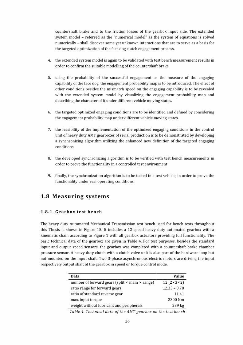
1.8 Measuring systems ............................................................................................................................................ 26
1.8.1 Gearbox test bench ....................................................................................................................................... 26
1.8.2 Test vehicle ...................................................................................................................................................... 28
2 Engaging capability of face dog clutches ............................................................................................................. 29
2.2 Analytical model ................................................................................................................................................. 30
2.2.1 Model equations ............................................................................................................................................ 30
2.2.2 Model results .................................................................................................................................................. 34
2.2.3 Model validation ............................................................................................................................................ 36
2.3 Numerical model ................................................................................................................................................ 38
2.3.1 Model equations ............................................................................................................................................ 38
2.3.3 Model implementation ............................................................................................................................... 45
2.3.4 Model validation ............................................................................................................................................ 46
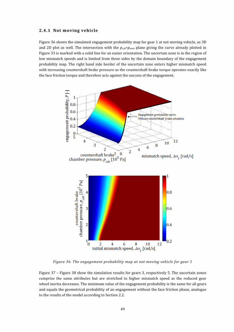
2.4 The engagement probability map ............................................................................................................... 48
2.4.1 Not moving vehicle ....................................................................................................................................... 49
7 Appendix A – Figures and Tables ............................................................................................................................ 79
7.2 Measurement results of the statistical evaluation ............................................................................... 80
7.3 Implementation of the numerical model in MATLAB/Simulink ................................................... 81
7.4 Implementation of the reverse time model in MATLAB/Simulink .............................................. 83
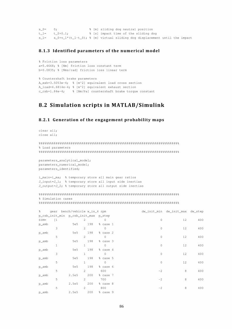
8 Appendix B – Program lists ....................................................................................................................................... 84
8.1.1 Analytical model ............................................................................................................................................ 84
8.1.2 Known parameters of the numerical model ..................................................................................... 85
8.1.3 Identified parameters of the numerical model ................................................................................ 86
8.2 Simulation scripts in MATLAB/Simulink................................................................................................. 86
8.2.1 Generation of the engagement probability maps ........................................................................... 86
8.2.2 Generation of the key regions and curves for not moving vehicle .......................................... 87
8.2.3 Generation of the key regions and curves for moving vehicle .................................................. 92
8.3 Visualization scripts for figures ................................................................................................................... 97
8.3.1 Script for Figure 12 ...................................................................................................................................... 97
8.3.2 Script for Figure 20- Figure 25 and Figure 33 - Figure 35 .......................................................... 98
8.3.3 Script for Figure 27 - Figure 30 ........................................................................................................... 101
8.3.4 Script for Figure 32 ................................................................................................................................... 105
8.3.5 Script for Figure 36 - Figure 40 ........................................................................................................... 107
8.3.6 Script for Figure 41 ................................................................................................................................... 110
8.3.7 Script for Figure 42 ................................................................................................................................... 110
8.3.8 Script for Figure 43 ................................................................................................................................... 111
8.3.9 Script for Figure 44 ................................................................................................................................... 112
8.3.10 Script for Figure 47 .............................................................................................................................. 113
8.3.11 Script for Figure 55 .............................................................................................................................. 114
8.3.12 Script for Figure 50- Figure 51 ....................................................................................................... 116
8.3.13 Script for Figure 56 .............................................................................................................................. 117
8.3.14 Script for Figure 57 .............................................................................................................................. 120
8
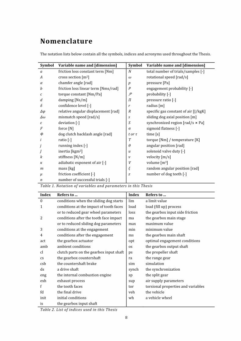
Nomenclature
The notation lists below contain all the symbols, indices and acronyms used throughout the Thesis.
Symbol Variable name and [dimension] Symbol Variable name and [dimension]
a friction loss constant term [Nm] N total number of trials/samples [-]
A cross section [m2] ω rotational speed [rad/s]
α chamfer angle [rad] p pressure [Pa]
b friction loss linear term [Nms/rad] P engagement probability [-]
c torque constant [Nm/Pa] � probability [-]
d damping [Ns/m] Π pressure ratio [-]
δ confidence level [-] r radius [m]
Δφ relative angular displacement [rad] R specific gas constant of air [J/kgK]
Δω mismatch speed [rad/s] s sliding dog axial position [m]
ε deviation [-] S synchronized region [rad/s ⨯ Pa]
F force [N] σ sigmoid flatness [-]
Φ dog clutch backlash angle [rad] t or τ time [s]
i ratio [-] T torque [Nm] / temperature [K]
j running index [-] θ angular position [rad]
J inertia [kgm2] u solenoid valve duty [-]
k stiffness [N/m] v velocity [m/s]
κ adiabatic exponent of air [-] V volume [m3]
m mass [kg] ξ random angular position [rad]
μ friction coefficient [-] z number of dog teeth [-]
n number of successful trials [-]
Table 1. Notation of variables and parameters in this Thesis
Index Refers to ... Index Refers to ...
0 conditions when the sliding dog starts lim a limit value
1 conditions at the impact of tooth faces load load (fill up) process
or to reduced gear wheel parameters loss the gearbox input side friction
2 conditions after the tooth face impact ma the gearbox main stage
or to reduced sliding dog parameters max maximum value
3 conditions at the engagement min minimum value
4 conditions after the engagement ms the gearbox main shaft
act the gearbox actuator opt optimal engagement conditions
amb ambient conditions os the gearbox output shaft
cl clutch parts on the gearbox input shaft ps the propeller shaft
cs the gearbox countershaft ra the range gear
csb the countershaft brake sim simulation
ds a drive shaft synch the synchronization
eng the internal combustion engine sp the split gear
exh exhaust process sup air supply parameters
f the tooth faces tor torsional properties and variables
fd the final drive veh the vehicle
init initial conditions wh a vehicle wheel
is the gearbox input shaft
Table 2. List of indices used in this Thesis
9
Acronym Acronym
AMT Automated Mechanical Transmission TCS Transmission Control Software
EEC Electronic Engine Control TCU Transmission Control Unit
ECU Electronic Control Unit
Table 3. List of acronyms used in this Thesis
List of Figures
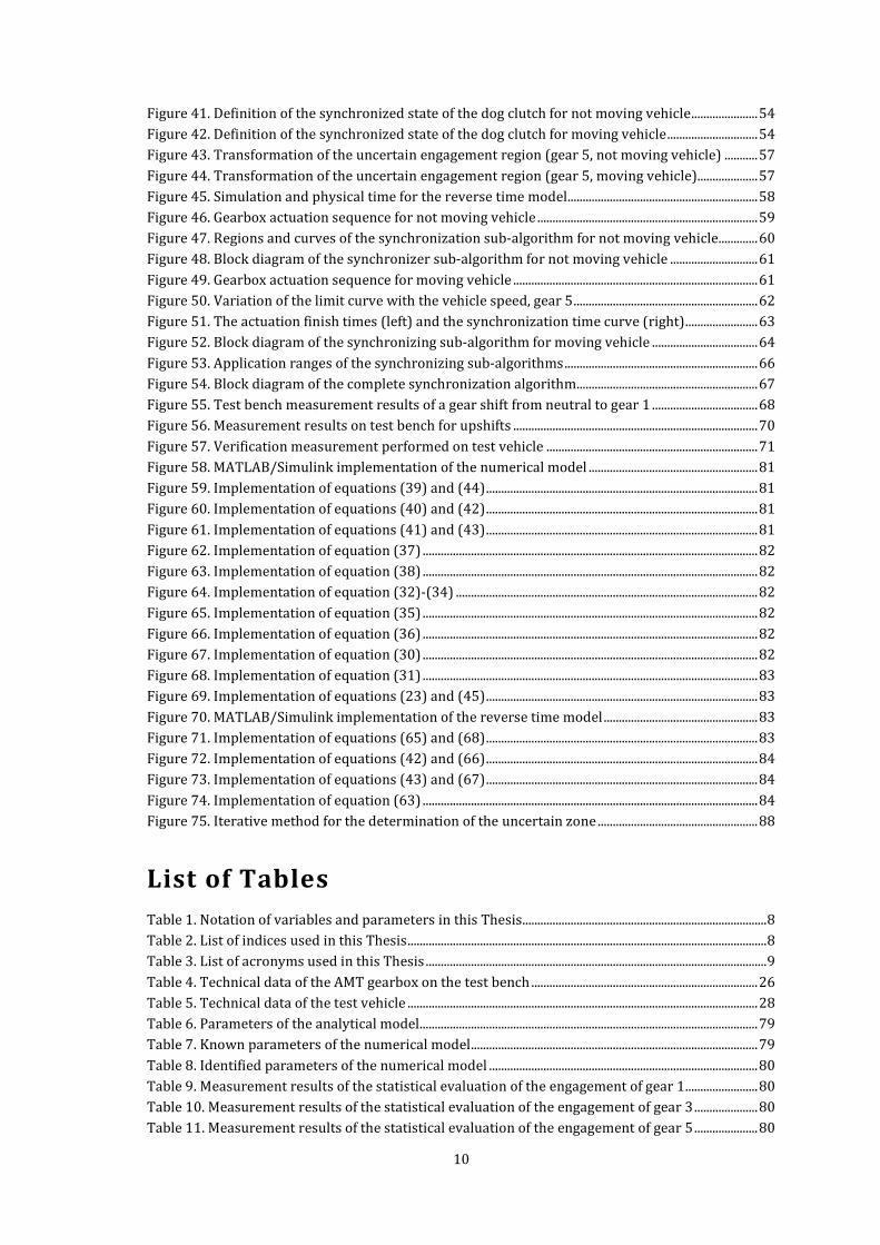
Figure 1.Kinematic chain of the driveline with a 12 speed heavy duty AMT ................................................ 11
Figure 2. Actuators and sensors of the Daimler GO 240-8 K “PowerShift” AMT ......................................... 12
Figure 3. Possible actuation sequences for upshifts at moving vehicle ........................................................... 14
Figure 4. Actuation sequence for gear shifts from neutral at not moving vehicle ...................................... 15
Figure 7. Electro-pneumatic countershaft brake with a fast evacuation valve [21] .................................. 17
Figure 8. Face dog clutch of the investigated gearbox............................................................................................. 19
Figure 9. Engagement process of face dog clutches ................................................................................................. 19
Figure 10. Effect of the mismatch speed on the engaging time of dog clutches [30] ................................. 21
Figure 11. Successful and unsuccessful face dog clutch engagement ............................................................... 22
Figure 12. Overview of the available mismatch speed zone ................................................................................. 23
Figure 13. Control algorithm for the countershaft brake based on rotational speed gradients [31]. 23
Figure 14. Control algorithm for the countershaft brake based on cut-off lead time [32] ..................... 24
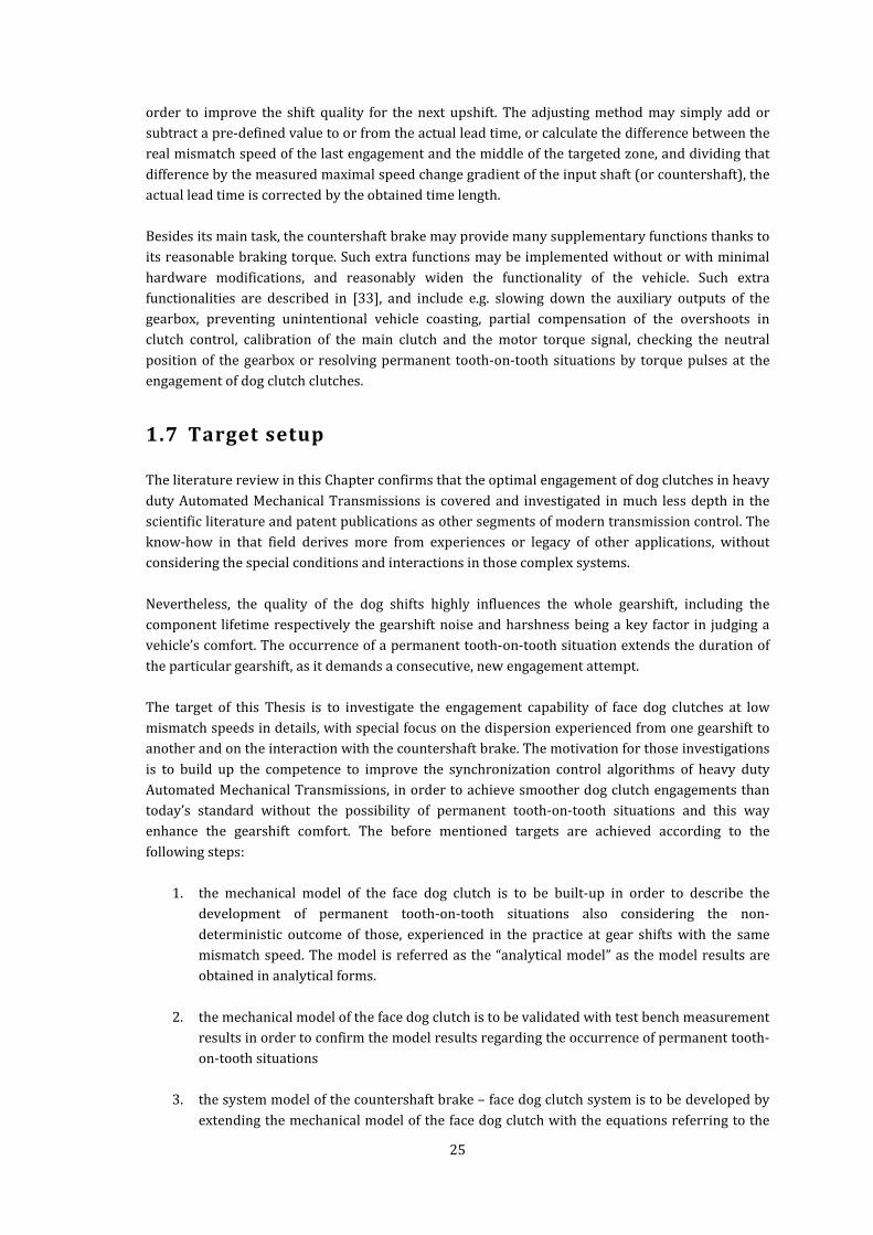
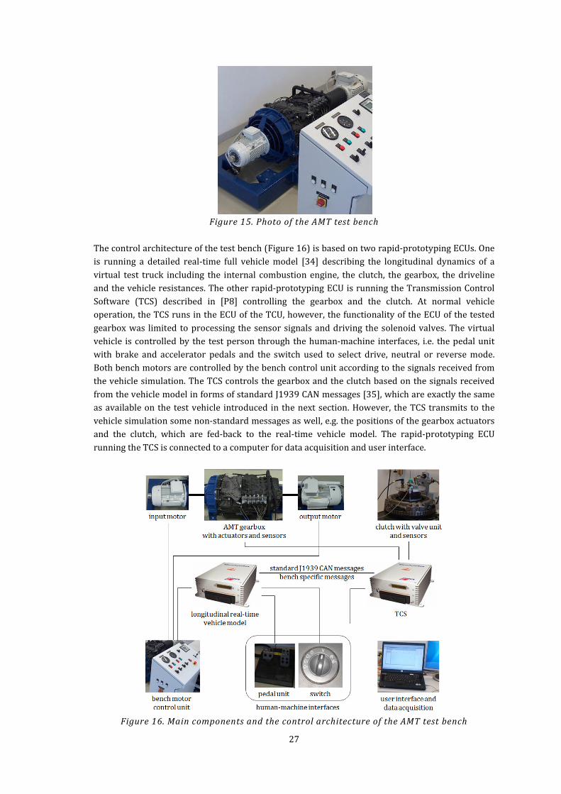
Figure 15. Photo of the AMT test bench ......................................................................................................................... 27
Figure 16. Main components and the control architecture of the AMT test bench .................................... 27
Figure 17. Control architecture on the test vehicle .................................................................................................. 28
Figure 18. Mechanical model of the dog clutch .......................................................................................................... 30
Figure 19. Relative initial position and its effect on the outcome of the engagement .............................. 32
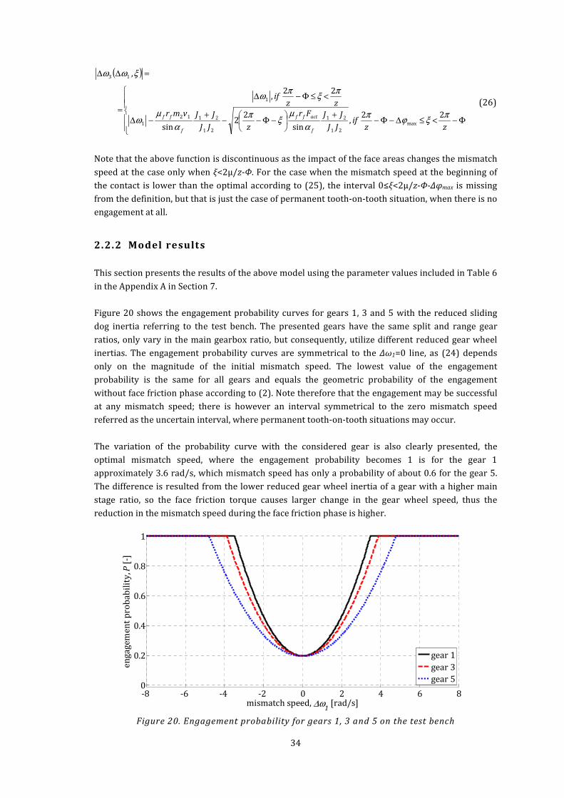
Figure 20. Engagement probability for gears 1, 3 and 5 on the test bench ................................................... 34
Figure 21. Comparison of the engagement probability of gear 5 on test bench and vehicle ................. 35
Figure 22. Mismatch speed at the engagement as a function of the random initial position................. 35
Figure 23. Model and measurement results for the engagement probability of gear 1 ........................... 37
Figure 24. Model and measurement results for the engagement probability of gear 3 ........................... 37
Figure 25. Model and measurement results for the engagement probability of gear 5 ........................... 37
Figure 26. The system model .............................................................................................................................................. 38
Figure 27. Identification of the gearbox input side friction losses .................................................................... 42
Figure 28. Identification of the countershaft brake torque constant ............................................................... 43
Figure 29. Identification of the load cross section .................................................................................................... 44
Figure 30. Identification of the exhaust cross section ............................................................................................. 44
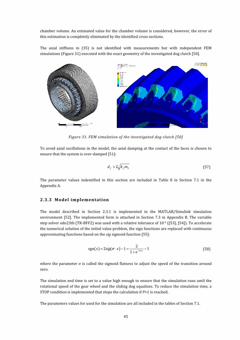
Figure 31. FEM simulation of the investigated dog clutch [50] ........................................................................... 45
Figure 32. Verification of a synchronization process .............................................................................................. 46
Figure 33. Model and measurement results for the engagement probability of gear 1 ........................... 47
Figure 34. Model and measurement results for the engagement probability of gear 3 ........................... 47
Figure 35. Model and measurement results for the engagement probability of gear 5 ........................... 47
Figure 36. The engagement probability map at not moving vehicle for gear 1 ........................................... 49
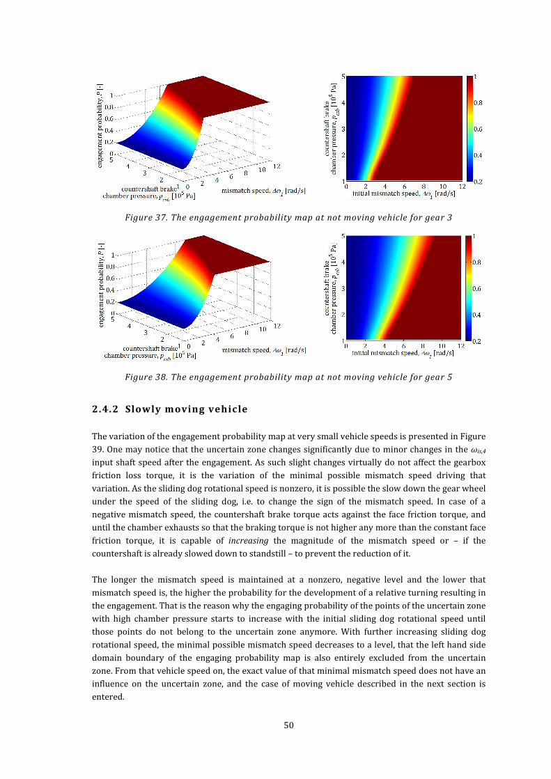
Figure 37. The engagement probability map at not moving vehicle for gear 3 ........................................... 50
Figure 38. The engagement probability map at not moving vehicle for gear 5 ........................................... 50
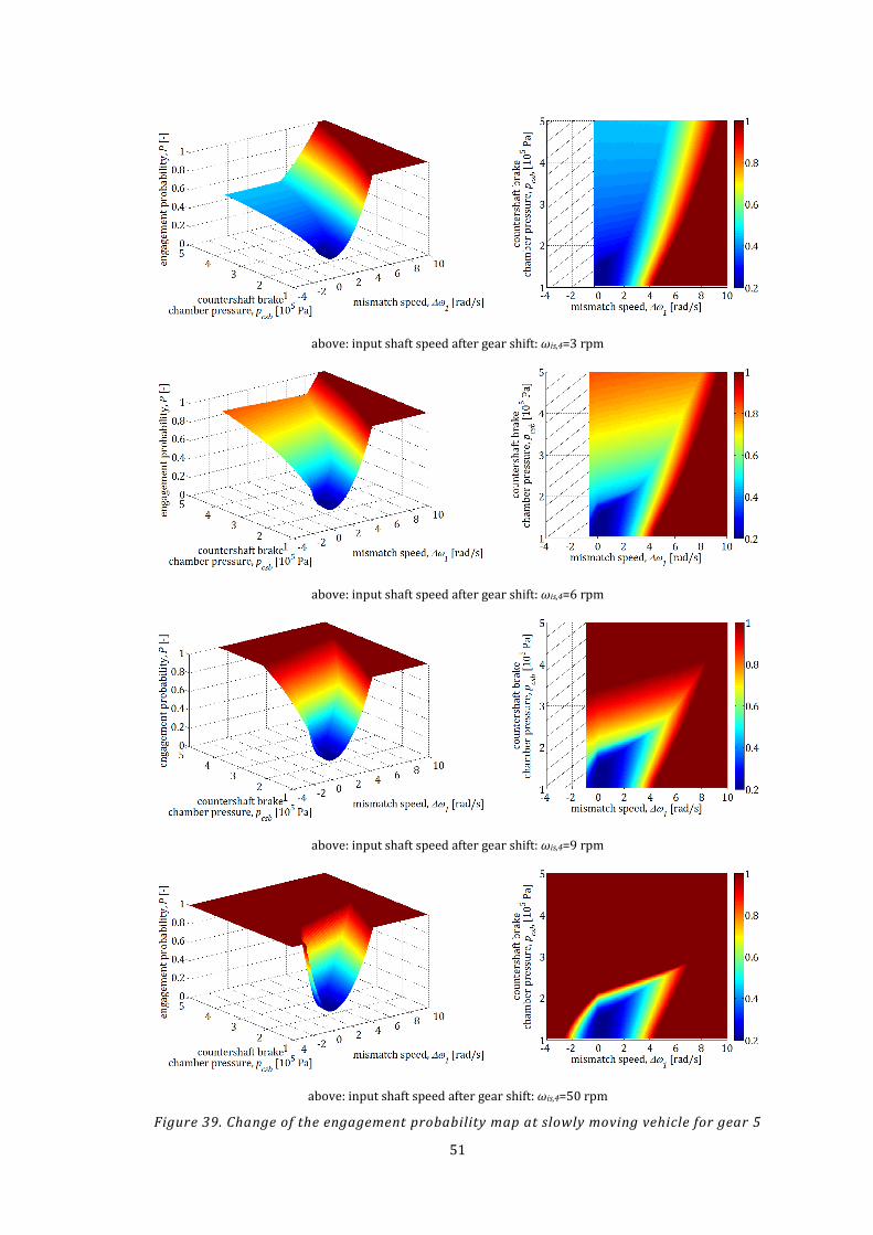
Figure 39. Change of the engagement probability map at slowly moving vehicle for gear 5 ................ 51
Figure 40. Change of the engagement probability map at moving vehicle for gear 5 ............................... 52
10
Figure 41. Definition of the synchronized state of the dog clutch for not moving vehicle ...................... 54
Figure 42. Definition of the synchronized state of the dog clutch for moving vehicle .............................. 54
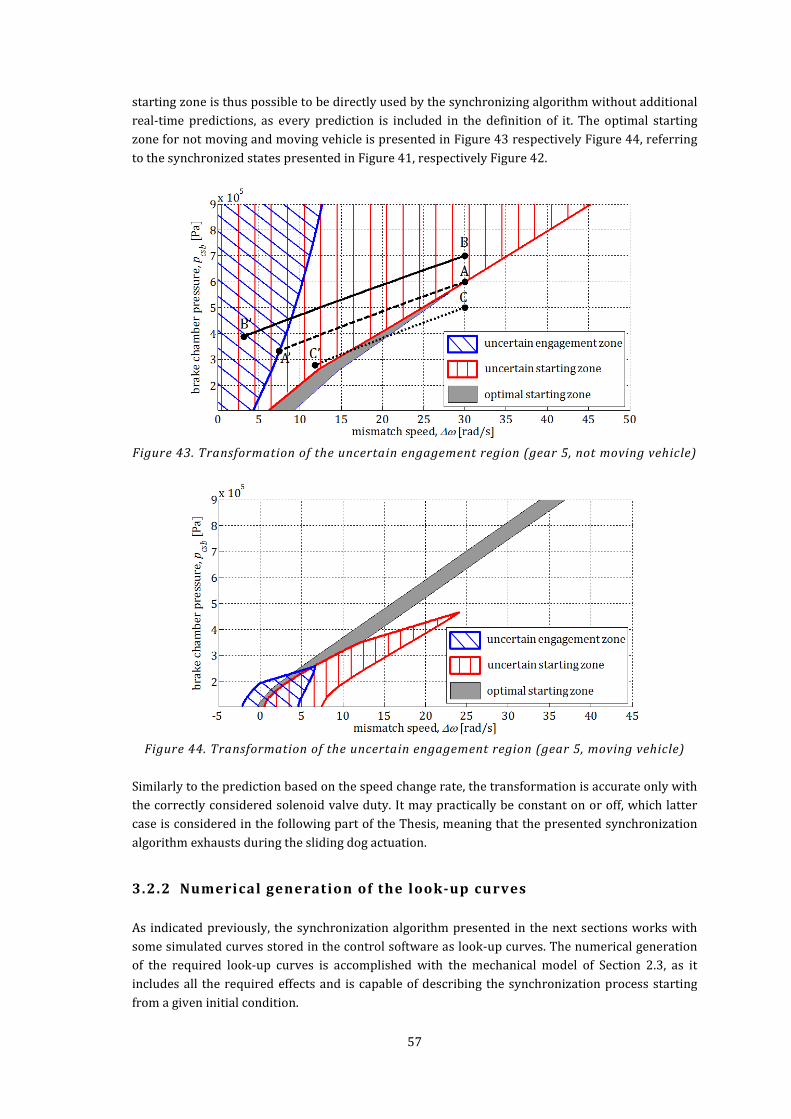
Figure 43. Transformation of the uncertain engagement region (gear 5, not moving vehicle) ........... 57
Figure 44. Transformation of the uncertain engagement region (gear 5, moving vehicle).................... 57
Figure 45. Simulation and physical time for the reverse time model............................................................... 58
Figure 46. Gearbox actuation sequence for not moving vehicle ......................................................................... 59
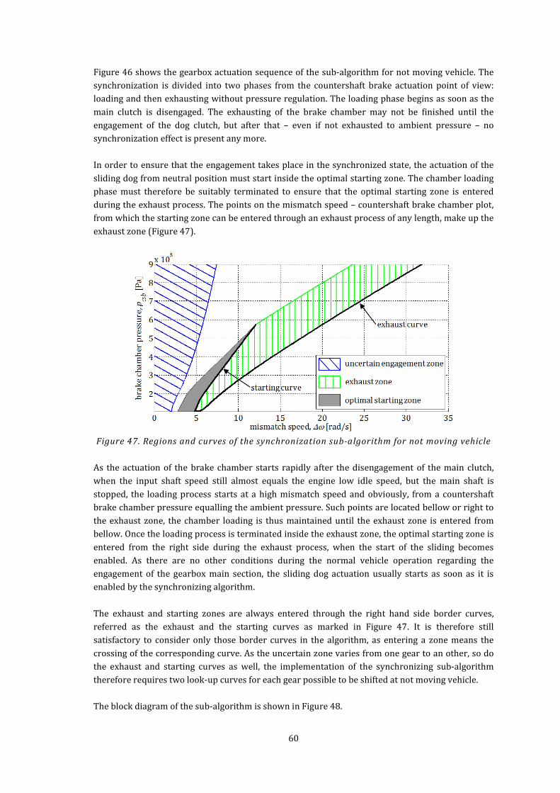
Figure 47. Regions and curves of the synchronization sub-algorithm for not moving vehicle............. 60
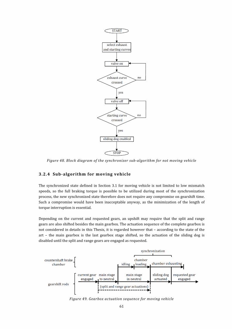
Figure 48. Block diagram of the synchronizer sub-algorithm for not moving vehicle ............................. 61
Figure 49. Gearbox actuation sequence for moving vehicle ................................................................................. 61
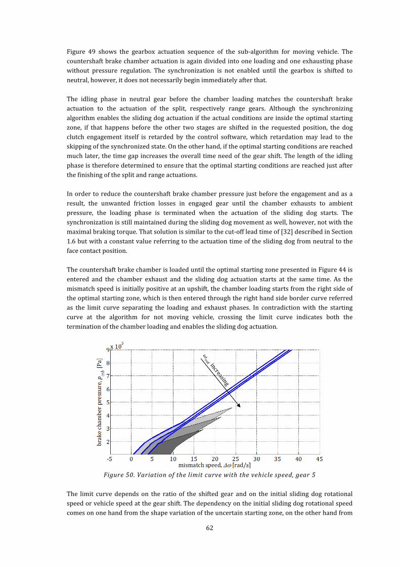
Figure 50. Variation of the limit curve with the vehicle speed, gear 5 ............................................................. 62
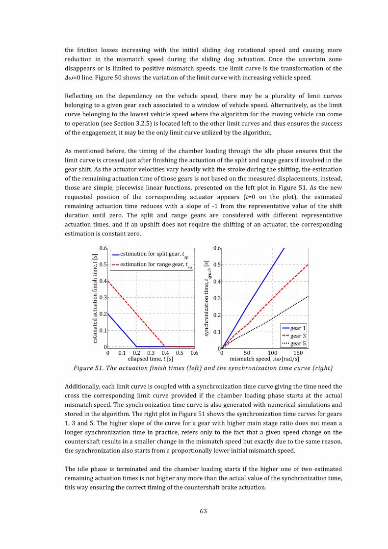
Figure 51. The actuation finish times (left) and the synchronization time curve (right) ........................ 63
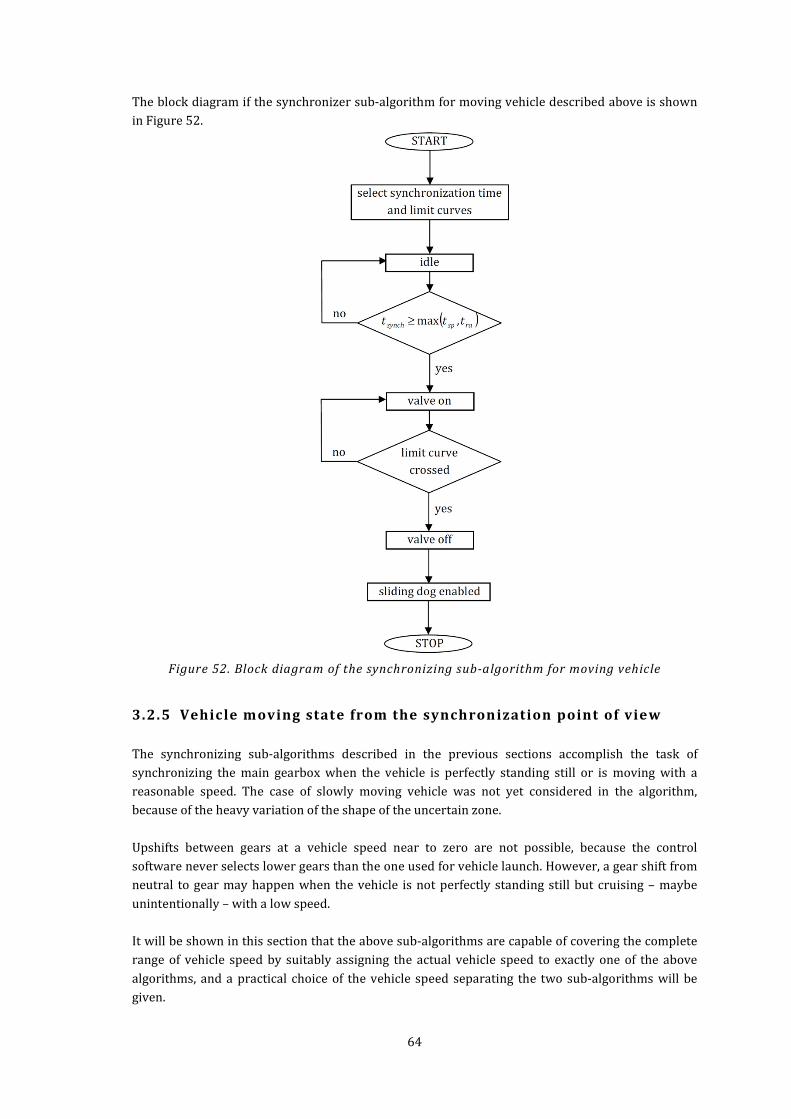
Figure 52. Block diagram of the synchronizing sub-algorithm for moving vehicle ................................... 64
Figure 53. Application ranges of the synchronizing sub-algorithms ................................................................ 66
Figure 54. Block diagram of the complete synchronization algorithm............................................................ 67
Figure 55. Test bench measurement results of a gear shift from neutral to gear 1 ................................... 68
Figure 56. Measurement results on test bench for upshifts ................................................................................. 70
Figure 57. Verification measurement performed on test vehicle ...................................................................... 71
Figure 58. MATLAB/Simulink implementation of the numerical model ........................................................ 81
Figure 59. Implementation of equations (39) and (44) .......................................................................................... 81
Figure 60. Implementation of equations (40) and (42) .......................................................................................... 81
Figure 61. Implementation of equations (41) and (43) .......................................................................................... 81
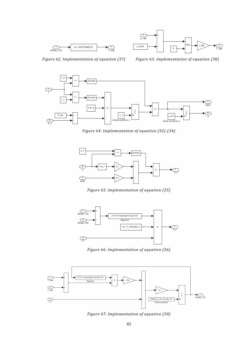
Figure 62. Implementation of equation (37) ............................................................................................................... 82
Figure 63. Implementation of equation (38) ............................................................................................................... 82
Figure 64. Implementation of equation (32)-(34) .................................................................................................... 82
Figure 65. Implementation of equation (35) ............................................................................................................... 82
Figure 66. Implementation of equation (36) ............................................................................................................... 82
Figure 67. Implementation of equation (30) ............................................................................................................... 82
Figure 68. Implementation of equation (31) ............................................................................................................... 83
Figure 69. Implementation of equations (23) and (45) .......................................................................................... 83
Figure 70. MATLAB/Simulink implementation of the reverse time model ................................................... 83
Figure 71. Implementation of equations (65) and (68) .......................................................................................... 83
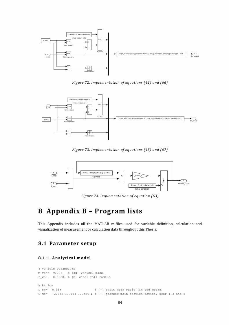
Figure 72. Implementation of equations (42) and (66) .......................................................................................... 84
Figure 73. Implementation of equations (43) and (67) .......................................................................................... 84
Figure 74. Implementation of equation (63) ............................................................................................................... 84
Figure 75. Iterative method for the determination of the uncertain zone ..................................................... 88
List of Tables
Table 1. Notation of variables and parameters in this Thesis ................................................................................. 8
Table 2. List of indices used in this Thesis ....................................................................................................................... 8
Table 3. List of acronyms used in this Thesis ................................................................................................................. 9
Table 4. Technical data of the AMT gearbox on the test bench ........................................................................... 26
Table 5. Technical data of the test vehicle .................................................................................................................... 28
Table 6. Parameters of the analytical model................................................................................................................ 79
Table 7. Known parameters of the numerical model ............................................................................................... 79
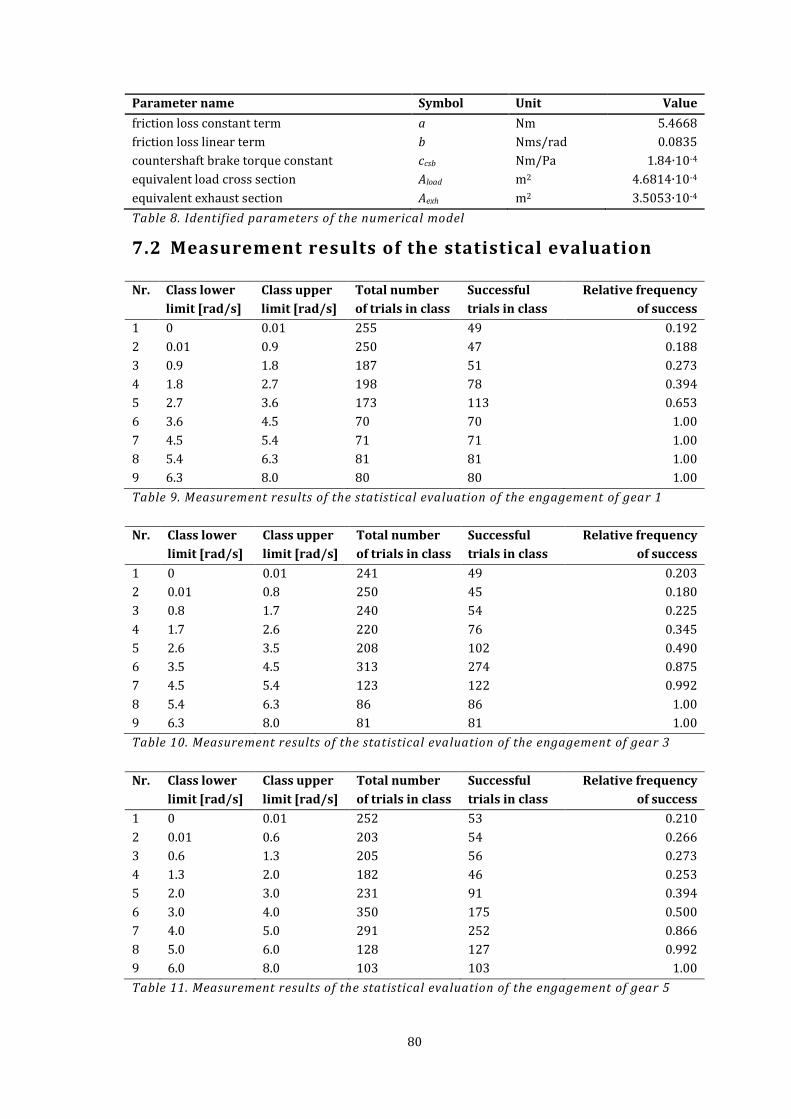
Table 8. Identified parameters of the numerical model ......................................................................................... 80
Table 9. Measurement results of the statistical evaluation of the engagement of gear 1 ........................ 80
Table 10. Measurement results of the statistical evaluation of the engagement of gear 3 ..................... 80
Table 11. Measurement results of the statistical evaluation of the engagement of gear 5 ..................... 80
11
1. Introduction
1.1 Heavy duty Automated Mechanical Transmissions
Despite enormous developments of the latest times, Automated Mechanical Transmissions with a
single dry clutch and a constant mesh gearbox still represent the state of the art compromise on
comfort and fuel efficiency in the category of heavy duty commercial vehicles. They combine the
efficiency of a manual gearbox and all the advantages of an automatic gearshift process. The latest
developments such as dual clutch transmissions – already matured for passenger car and light duty
commercial vehicle applications [1] – yet fail to meet the extreme load, lifetime and efficiency
requirements of the heavy duty category.
Figure 1.Kinematic chain of the driveline with a 12 speed heavy duty AMT
To achieve the high number of forward gears – typically 12-18 – required for fuel optimal operation
under full load with a comparatively low number of gearwheel pairs, automated heavy duty
gearboxes – as the manual ones – are generally designed with three stages having split and range
gears before, respectively after the main gearbox, all integrated in a common housing. Except for
atypical designs with a 3-speed range group, the split and range groups have two gears each, the
gears of the main gearbox including reverse are this way quadrupled (Figure 1). The range gear is
usually a planetary gear set, to ensure a huge ratio step but still a very good mechanical efficiency at
locked state in the upper gears, when its ratio is 1. The input shaft can be directly coupled with the
main shaft enabling an extreme efficient direct drive in the highest or second highest gear. Some
gearboxes are built with a twin countershaft design principle ([2], [3]), where the power flow is
split among the two identical countershafts reducing the spline load. The neutral of the whole
gearbox is achieved through the neutral gear of the main gearbox, because – except for some
gearboxes with extended functionality, e.g. the Eco-Roll function [4] – neither the split nor the
range gear can be shifted into neutral.
The clutch and the gearshift rods are not actuated manually by the driver, but through actuators
(Figure 2) controlled electronically by a joint Transmission Control Unit (TCU). As the compressed
12
air system is implemented in heavy duty vehicles for the brake system anyway, the transmission is
also actuated mainly electro-pneumatically, alternatively electro-mechanically (e.g. [P7]) or electro-
hydraulically. The clutch actuator may be placed concentrically to the gearbox input shaft or may
act on the clutch plate through a lever arm mechanism, as in Figure 2. The gearshift rod actuators
may be integrated with the TCU electronic in a common unit or may be placed on the gearbox
housing individually. The split and range gears require one actuator each, while the main gearbox
usually requires two of them. Depending on the gearbox’ design, the main gearbox may have two or
three identical parallel main shift actuators or one main shift and one select (or gate) actuator, the
latter is placed perpendicular to the main shift actuator, dimensioned usually smaller and selects
the shifting fork to be shifted through the main shift actuator.
Figure 2. Actuators and sensors of the Daimler GO 240-8 K “PowerShift” AMT
(8-speed bus and coach application without range gear, [5])
In order to recognize the vehicle’s operating condition, respectively driving situation and this way
to determine the optimal gear, the TCU software ([6]-[8]) processes the signals of the transmission-
related sensors (e.g. clutch position, gearshift rod positions, gearbox shaft speeds, road climb angle,
etc.) and those available on the vehicle’s CAN communication system. By overriding the Electronic
Engine Control (EEC) for the short periods of the gear shifts, the TCU is capable of accomplishing
gear changes without any driver interaction.
1.2 Synchronization of heavy duty Automated Mechanical
Transmissions
To build up the new power-flow path referring to the requested new gear, some gear wheels have
to be released from their shaft, while others have to get fixed to it by means of dog clutches (see
Section 1.5) in form of a shape-locking connection between the gear wheel and the corresponding
shaft. Before engaging a dog clutch, the speed difference between the engaging parts has to be
reduced, which process is known as synchronization. In this Thesis, the synchronized state of a dog
clutch with synchromesh ([9] - [11]) is understood as the perfectly synchronized state i.e. when the
mismatch speed is zero. When referring to the synchronized state with respect to a dog clutch
13
without synchromesh, it is understood as a partially speed-synchronized state, when the engaging
conditions are suitable to ensure the comfort and component lifetime requirements.
When the gearbox is in neutral, it is separated to input and output sides, made of the gearbox parts
before, respectively after the dog clutch to be engaged. The speed of the output side is determined
by the vehicle speed, so it is the speed of input side that has to be manipulated during the
synchronization. In case of synchromesh, the input side speed is matched through the
synchronizing torque transmitted by the friction surfaces of the synchronizer ring. In case of an
AMT, however, the transmission control enables the modification of the input side speed and thus
the synchronization without the synchronizing torque of the synchromesh as well.
During gear shifts, the TCU overrides the EEC to control the engine speed to the level required in
the gear to be shifted, which speed – assuming that the split gear has already been shifted –
corresponds to the perfectly synchronized speed of the countershaft, anyway. The input shaft speed
can quickly be matched to the controlled engine speed through partial or full clutch engagment – if
previuosly disengaged – to synchronize the main gearbox. However, even engines with advanced
engine brake systems have slower dynamics for speed reduction as for speed increase. Therefore at
upshifts, when the input shaft has to be slowed down to reach the synchronized speed, the speed
reduction is usually aided or with disengaged clutch accomplished alone by a countershaft brake
acting on the countershaft (Figure 1). The countershaft brake is an additional gearbox actuator, and
also comes in operation when shifting from neutral to a gear at not moving vehicle, to slow down
the input shaft from the engine low idle speed more quickly than purely the friction losses would
do.
AMT gearboxes – unlike manual ones – thus have a centrally synchronized main gearbox with dog
clutches without synchromesh. The omission of the synchronizer rings and other synchromesh
parts reduces the mechanical complexity and installation space therefore enables the widening of
gearwheel width within the same gearbox housing. That increases the weight/power ratio or
specific weight of the gearbox, which is of high priority because of today’s overall weight reduction
efforts in order to reduce the fuel consumption or to increase the payload. The synchromesh of the
split gear is however not replaced with dog clutches, because the small speed differences resulted
by the small ratio step of the split gear is quicker and easier to be synchronized internally.
Furthermore, the synchromesh of the range gear is not omitted either, but for an opposite reason:
the ratio step of the range gear is higher than the ratio of the engine’s low and high idle speeds, so
the main shaft speed range required for the synchronization is not possible to be covered with
engine speed change.
As a development expected to be introduced in the next couple of years, the standard heavy duty
Automated Mechanical Transmissions may optionally be extended with a powershift module (e.g.
[12], [13]) enabling the shifting without torque interruption between at least the highest two gears.
The motivation behind is the reduction of fuel consumption through lower engine revolution at the
highest vehicle speed achieved by longer final drive ratio, which however results in more frequent
gear shifts between the highest two gears. The loss of torque interruption during just those gear
shifts makes those shifts virtually unnoticeable for the driver, and this way eliminates the reduction
of driveability. The extension refers only to the split gear; the main gearbox including the
countershaft brake remains principally unchanged.
14
1.3 Gearshift sequences with countershaft brake
actuation
Based on tradition, legacy or core competence and constrained by the protected intellectual
properties of the competitors, the major transmission manufacturers have developed different
sequences for the gearshift processes. Those sequences are sometimes completely different from
each other, however, provide practically the same functionality and comfort from the driver’s point
of view. Regardless of the manufacturer, every gearshift sequence involving the gearbox main stage
has the following 6 main steps:
1. releasing the driveline torque,
2. shifting the main gearbox into neutral,
3. shifting the split and range gears, if involved in the gear shift,
4. synchronizing the dog clutch to be engaged,
5. engaging the dog clutch,
6. building up the driveline torque to the level demanded by the driver.
Figure 3. Possible actuation sequences for upshifts at moving vehicle
As the engaging devices are only hardly or not at all possible to be disengaged under load, the
torque in the driveline has to be reduced as the first step of the gearshift process. The one way to
reduce the torque is an active torque control method using the internal combustion engine as an
actuator. For that method the main clutch remains engaged for all the time, and the torque-free
state of the dog clutch to be disengaged in the main gearbox is accomplished by a state-feedback
engine fuel injection control where the fed-back signals usually come from state observers ([14]-
[16]). The synchronization of the dog clutch to be engaged is done by proper speed control of the
engine optionally aided by the countershaft brake, and after engagement, the driveline torque is
built-up again using engine torque control. As such a sequence (Figure 3a) requires a very
advanced competence in engine control, it is usually used only when the disengagement of the
clutch before gear shifts is not possible, for example because the vehicle is equipped with a
centrifugal clutch which is permanently engaged above a certain engine speed [17], or with a
manual clutch. The combination of manual clutch and automated gearbox is typical for one specific
15
truck manufacturer; however, its newest system comprises an automated clutch as an option which
is disengaged before gear shifts [18].
The other and more conventional way of driveline torque reduction is the disengagement of the
main clutch. In that case as well, the engine torque has to be ramped down before the clutch
disengagement, to avoid the heavy oscillations and vehicle jerk appearing in case of a too quick
torque release. That torque ramp-down however can be achieved simply, without regulation. Once
the driveline is open and the main gearbox in neutral, the speed synchronization of the dog clutch
to be engaged may happen at engaged (Figure 3b) or disengaged clutch (Figure 3c).
The first method is used when the engine is equipped with an effective engine brake system, and in
that case the clutch engages at neutral gear and the speed reduction of the input shaft is
accomplished together with the engine and countershaft brakes ([19], [20]). The new gear is
engaged at closed main clutch, and finally the driveline torque is built up by engine torque control.
According to the method in Figure 3c, the speed synchronization of the dog clutch to be engaged is
done by the countershaft brake alone, and the engagement of the new gear happens also at
disengaged clutch ([3], [21]). After that, the clutch engages and the driveline torque is built up by
engine torque control. That method is the most similar to the driver’s action at manual gearboxes,
and is advantageous if the engine is not equipped with an effective engine brake system and thus
the speed reduction rate is more limited. The speed of the engine required in the new gear has to be
reached namely only after the engagement of the new gear, at the other two methods however,
before that. Another difference from the other two methods is that the engagement of the dog
clutch takes place at disengaged main clutch.
If the split or range gear is also involved in the gear shift, those are shifted after the driveline torque
release and before the synchronization of the main gearbox.
Figure 4. Actuation sequence for gear shifts from neutral at not moving vehicle
Though the gearshift sequence for upshifts at moving vehicle varies among the transmission
manufacturers, the sequence for gear shifts from neutral to gear at not moving vehicle always
follows the same scheme (Figure 4). As the synchronization of such gear shifts require that the
input shaft speed is reduced close to zero i.e. well below the engine low idle speed, the engine
cannot be used for synchronization purposes. When the gearbox is in neutral gear, the clutch is
16
usually engaged which is the so-called normal, not actuated position of the clutch. As soon as a gear
shift is required, first the clutch is disengaged. While the engine maintains the low idle speed, the
speed of the input shaft and that of the countershaft begins to slowly decrease towards zero due to
the friction losses, however, in order to achieve an acceptable gear shift time, the countershaft
brake is also used to accelerate the speed reduction.
Consequently, the countershaft brake is mandatory for all gearboxes with centrally synchronized
main gearbox even if gear shifts at moving vehicle do not require the actuation of it.
1.4 Prior art of countershaft brake design
As described in the previous sections, the countershaft brake is a common synchronizing device for
all the dog clutches of the main gearbox capable of reducing the speed of the countershaft and used
for synchronization at gear shifts from neutral to gear at not moving vehicle and eventually, for
upshifts at moving vehicle. Gearbox brakes with the same function are already known from old
fashioned, unsynchronized manual heavy duty gearboxes, mounted on the input shaft and activated
by the driver through over-pressing the clutch pedal. The countershaft brake of a heavy duty
Automated Mechanical Transmission is supervised by the TCU and is actuated in most cases – as
the shift actuators – electro-pneumatically.
Figure 5. Countershaft brake discs
A countershaft brake usually comprises a plurality of friction discs (Figure 5) with outer,
respectively inner grooves alternately and friction linings usually mounted on every 2nd disc. The
standard design is shown in Figure 6, where the discs with inner grooves are non-rotatably fixed to
the countershaft, the discs with outer grooves but to the cap mounted on the gearbox housing.
When the countershaft brake is activated i.e. the chamber is pressurized, the piston pushes the
friction discs against a plate, generating a brake torque acting on the countershaft with respect to
the gearbox housing. When the chamber is not pressurized, a release spring holds the piston in the
idle position where the piston has no contact with the discs. A countershaft brake can typically
provide a maximal brake torque of 100-120 Nm, resulting in a deceleration of the countershaft of
up to 5000 rpm/s.
In practice, the countershaft brake chamber is usually pressurized and exhausted through a 3-by-2
control solenoid (Figure 6), which means that the chamber is either loaded or open to the
atmosphere without the possibility the hold a pressure level in the chamber different from the
supply or the ambient pressure.
17
Figure 6. Today’s standard electro-pneumatic countershaft brake design [22]
Figure 7 shows an alternative solution with an evacuation valve also in serial production. In this
case, the chamber is pressurized though a 2-by-2 control solenoid and exhausted through the
evacuation valve made up of only a rubber body which closes the exhaust opening if the control
solenoid is activated. It is possible to be designed with a much higher cross section as a control
solenoid, which means a reasonable reduction in the exhaust times. However, apart from the cross
sections, the system is pneumatically equivalent to the one shown in Figure 6.
Figure 7. Electro-pneumatic countershaft brake with a fast evacuation valve [21]
The design with the friction discs presented on the above figures is the most commonly used;
however, it has some reasonable disadvantages. One of them is the friction loss at the idle state of
the countershaft brake. Though the piston is released by the release spring, the friction discs are
not completely separated from each other, and are continuously producing a slight braking torque.
The other source of the losses is the release spring itself, as it is on one end supported by the piston
mounted in the stationary cap, on the other end it is supported by the rotating countershaft, which
speed difference also causes some friction loss. The other disadvantage of the presented design is
18
the large number of parts, the complex assembly and the difficult repair process which requires the
complete disassembly of the main clutch.
There are many design solutions typically in patent application publications (e.g. [22] - [27]), which
refer to alternative actuation principles, simplification of the assembly or installation, reduction of
unwanted friction losses or characterize a self-energizing design. A possible future evolution of the
countershaft brake may be like described in [28] referred as the central synchronizer capable of
synchronizing all gears at both up- and downshifts. However, the kinematic layout of such a
gearbox with a central synchronizer is merely different from today’s heavy duty standard and such
a gearbox is not in serial production so far.
1.5 Dog clutches in heavy duty Automated Mechanical
Gearboxes
As dog clutches are nowadays almost exclusively provided with synchromesh in passenger car
applications being the only application known and used by most of the car drivers, the idea of using
dog clutches without synchromesh in state-of-the-art automotive gearboxes may seem unfamiliar.
The benefits of synchromesh are the inherent synchronization and interdiction features (e.g. [9]-
[11]), which means that the speed synchronization of the meshing elements comes without
external intervention, and the engagement is blocked until the speed synchronization is finished.
Disadvantages are the long time required for the complete speed synchronization and the
additional elements such as synchronizer rings or detents ([P6]) that have to be included in every
single engaging device separately even for those that cannot be engaging simultaneously. For
applications, where the required additional installation space or the comparatively long
synchronization time is not acceptable, synchromesh gearboxes are not welcomed. Such
applications, where the development of dog clutches without synchromesh is still ongoing [29], are
the following:
� motorcycles, where there is no room for synchromesh inside the gearbox, but thanks to the
very low gearbox inertias, unsynchronized engagements cause only low torsional
vibrations, so the loss of synchronization does not mean a real loss of lifetime and drive
comfort, especially, considering the inherently crude nature of riding, anyway,
� race cars, where comfort is not an aspect at all and the torque interruption during gear
shift has to be kept minimal at all costs, so the extension of gearshift time is not acceptable,
and
� heavy duty commercial vehicles with Automated Mechanical Transmission, where after a
sidetrack to synchromesh gearboxes, it has been realized, that the latest requirements
regarding the power/weight ratio, lifetime and gearshift speed cannot be fulfilled with
synchromesh. However, the large inertias call for at least partial synchronization
accomplished by transmission control in order to achieve suitable engaging conditions for
the dog clutches to fulfil the demanding comfort and lifetime requirements.
Dog clutches in general are simple locking coupling devices made up of two engaging elements used
to lock a driveline element, usually a gear wheel to its shaft. Both engaging elements are provided
with meshing geometry in forms of teeth and slots. The first engaging element called as sliding dog
or sleeve is locked to the shaft in a torque secure manner, but can be displaced axially through the
19
corresponding shift fork. The second engaging element is generally integrated in the gear wheel.
The locking or the engagement is realized through the meshing teeth when the sliding dog is in the
engaged axial position.
The slots between the meshing teeth are either cut on the inner or outer cylindrical surface parallel
to the centre axis of the dog clutch or on the face surface manufactured in radial direction.
However, the placement of the slots does not play an important role in the engaging characteristics
of the dog clutch; essential is the geometry of the tooth faces. From that aspect, dog clutches can be
divided into two basic types: standard and face dog clutches [30].
Figure 8. Face dog clutch of the investigated gearbox
The ending of the teeth of standard dog clutches utilize nose angle on both engaging elements
forming arrows usually with cut-backs as well. The teeth of face dog clutches have flat face areas,
the face areas of the sliding dog and the gear wheel are thus possible to slide on each other. The
geometry of the dog clutch in the gearbox investigated in this Thesis is shown in Figure 8. That is a
face dog clutch, with slots parallel to the centre axis, and as a special feature, with edge chamfer on
the face areas, which are consequently small pieces of the same conical surface.
Figure 9. Engagement process of face dog clutches
20
As there is no interdiction feature, the engagement of a dog clutch can take place at any speed
difference between the gear wheel and the sliding dog, which difference is referred as the mismatch
speed. The stages of the engagement process of a face dog clutch are shown in Figure 9. The
actuation of the sliding dog starts at t0 time when the mismatch speed has a value of Δω0. The dog
clutch transmits no torque, and the engagement phase is called free fly, lasting until the sliding dog
reaches the gear wheel at t1 time. Because of the possible minor changes in vehicle speed and more
importantly, due to the friction losses and the eventual countershaft brake torque acting on the
gear wheel, the mismatch speed changes to Δω1 by that time. It is usually the tooth faces which first
come in contact, resulting in an impact. The high impact force peak stops the sliding dog by
consuming the motion energy of the whole actuation mechanism attached to it. The normal force
between the sliding dog and the gear wheel and the relative turning of them imply a face friction
torque acting against the relative turning. As the peak in the normal force results in a peak in the
face friction torque as well, the mismatch speed reduces to Δω2 in the negligible t2-t1≈0 time range
of the face impact. After the impact, the face areas slip on each other, until the teeth turn against the
slots by the time t3. That phase is called the face friction phase, and the face friction torque still
acting against the relative turning further reduces the mismatch speed to Δω3. As the teeth of the
sliding dog are now free to enter the slots the gear wheel, the dog clutch engages, and the mismatch
speed quickly reduces to zero provoking heavily damped torsional vibrations in the driveline
lasting only a few cycles. The peak value of those vibrations can be estimated based on the
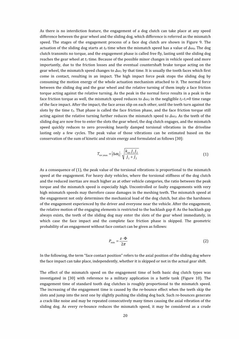
conservation of the sum of kinetic and strain energy and formulated as follows [30]:
21
213max, JJ
JJkT tor
tor+
⋅∆= ω (1)
As a consequence of (1), the peak value of the torsional vibrations is proportional to the mismatch
speed at the engagement. For heavy duty vehicles, where the torsional stiffness of the dog clutch
and the reduced inertias are much higher as at other vehicle categories, the ratio between the peak
torque and the mismatch speed is especially high. Uncontrolled or faulty engagements with very
high mismatch speeds may therefore cause damages in the meshing teeth. The mismatch speed at
the engagement not only determines the mechanical load of the dog clutch, but also the harshness
of the engagement experienced by the driver and everyone near the vehicle. After the engagement,
the relative motion of the engaging elements is restricted to the backlash gap θ. As the backlash gap
always exists, the teeth of the sliding dog may enter the slots of the gear wheel immediately, in
which case the face impact and the complete face friction phase is skipped. The geometric
probability of an engagement without face contact can be given as follows:
π2min
Φ⋅=
zP (2)
In the following, the term “face contact position” refers to the axial position of the sliding dog where
the face impact can take place, independently, whether it is skipped or not in the actual gear shift.
The effect of the mismatch speed on the engagement time of both basic dog clutch types was
investigated in [30] with reference to a military application in a battle tank (Figure 10). The
engagement time of standard tooth dog clutches is roughly proportional to the mismatch speed.
The increasing of the engagement time is caused by the re-bounce effect when the teeth skip the
slots and jump into the next one by slightly pushing the sliding dog back. Such re-bounces generate
a crack-like noise and may be repeated consecutively many times causing the axial vibration of the
sliding dog. As every re-bounce reduces the mismatch speed, it may be considered as a crude
21
synchronization. A re-bounce may also occur at face dog clutches as well, but usually only at
extreme high mismatch speeds which are not likely in normal operation.
Figure 10. Effect of the mismatch speed on the engaging time of dog clutches [30]
In contradiction to standard tooth dog clutches, the engagement time of face dog clutches is not
determined by the mismatch speed. Reason is that the length of the face friction phase varies from
one gearshift to another depending on the relative turning required for the sliding dog to enter the
slots of the gear wheel. The engaging time at a given mismatch speed is characterized by an interval
with the minimum value referring to the engagement without face contact with engaging time
corresponding only to the axial dynamics of the sliding dog, thus independent from the mismatch
speed, and with maximum value referring to the engagement with the largest possible relative
turning required for the engagement.
The graph in Figure 10 however refers to dog shifts with high mismatch speed at the engagement.
As already described, despite the lack of synchromesh, the mismatch speed of dog clutches in heavy
duty automated gearboxes is reduced independently from the engaging device to a suitably low
level, so the engaging conditions are different from other dog clutch applications and not included
in Figure 10.
As the mismatch speed is reasonably reduced in the disengaged state of the dog clutch and is
further decreased by the face friction torque, it may be completely vanished during the face friction
phase before the engagement. The result is a permanent tooth-on-tooth situation, when the face
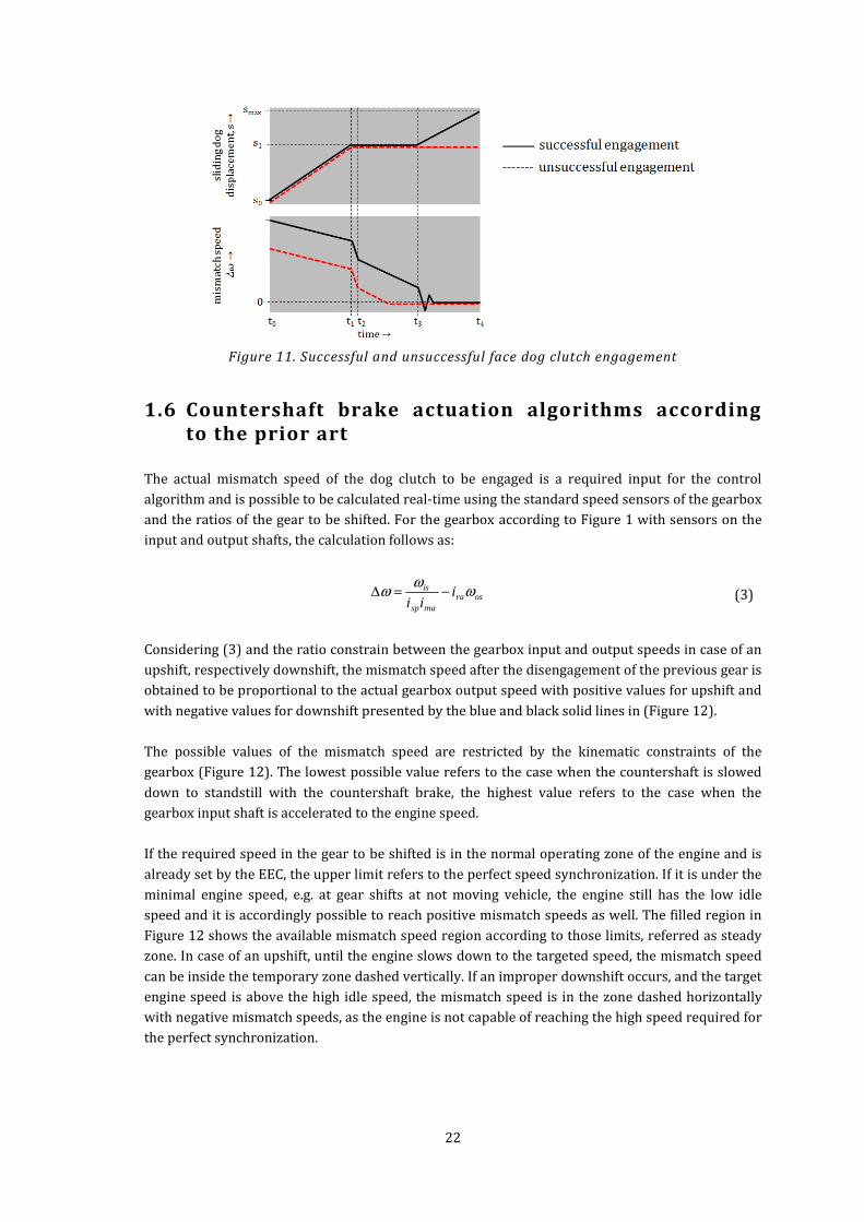
contact is not resolved and the stroke of the sliding dog cannot be completed (Figure 11).
Permanent tooth-on-tooth situations play an important role in transmission control, as those are
the most frequent reason when an engagement attempt is unsuccessful in a heavy duty Automated
Mechanical Transmission. It is obvious, that lower mismatch speeds are suitable for the
development of such situations, but the occurrence is not determined by the mismatch speed alone,
as it is also influenced by the relative turning required for the sliding dog during the phase friction
phase to enter the slots of the gear wheel.
22
Figure 11. Successful and unsuccessful face dog clutch engagement
1.6 Countershaft brake actuation algorithms according
to the prior art
The actual mismatch speed of the dog clutch to be engaged is a required input for the control
algorithm and is possible to be calculated real-time using the standard speed sensors of the gearbox
and the ratios of the gear to be shifted. For the gearbox according to Figure 1 with sensors on the
input and output shafts, the calculation follows as:
osramasp
is iii
ωω
ω −=∆ (3)
Considering (3) and the ratio constrain between the gearbox input and output speeds in case of an
upshift, respectively downshift, the mismatch speed after the disengagement of the previous gear is
obtained to be proportional to the actual gearbox output speed with positive values for upshift and
with negative values for downshift presented by the blue and black solid lines in (Figure 12).
The possible values of the mismatch speed are restricted by the kinematic constraints of the
gearbox (Figure 12). The lowest possible value refers to the case when the countershaft is slowed
down to standstill with the countershaft brake, the highest value refers to the case when the
gearbox input shaft is accelerated to the engine speed.
If the required speed in the gear to be shifted is in the normal operating zone of the engine and is
already set by the EEC, the upper limit refers to the perfect speed synchronization. If it is under the
minimal engine speed, e.g. at gear shifts at not moving vehicle, the engine still has the low idle
speed and it is accordingly possible to reach positive mismatch speeds as well. The filled region in
Figure 12 shows the available mismatch speed region according to those limits, referred as steady
zone. In case of an upshift, until the engine slows down to the targeted speed, the mismatch speed
can be inside the temporary zone dashed vertically. If an improper downshift occurs, and the target
engine speed is above the high idle speed, the mismatch speed is in the zone dashed horizontally
with negative mismatch speeds, as the engine is not capable of reaching the high speed required for
the perfect synchronization.
Figure 12
The countershaft brake control algorithms according to the prior art
of the gearbox input shaft or what is the same, that of the countershaft towards the level
corresponding to the perfectly synchronized speed of the input shaft (or countershaft) until a pre
defined target mismatch speed window
entered. The targeted zone is near the zero mismatch speed, but usually does not include it.
Figure 13. Control algorithm for the
Since it is not the start of the sliding dog but the engagement of the dog clutch which should take
place inside that target zone,
regarding the time of reaching the synchronized state, which estimations are then used to control
the actuation of the sliding dog.
of the gearbox input shaft (or countershaft) and the gearbox output shaft (
is the time dependent target rotational speed of the gearbox
calculated from the actual driving speed of the vehicle
gearbox. The time dependency is caused by the slight changes in the speed of the vehicle running
freely with disengaged clutch caused by the air drag and road resistances (including road climbing
23
12. Overview of the available mismatch speed zone
control algorithms according to the prior art upon request
of the gearbox input shaft or what is the same, that of the countershaft towards the level
corresponding to the perfectly synchronized speed of the input shaft (or countershaft) until a pre
smatch speed window considered as the synchronized state of the dog clutch
The targeted zone is near the zero mismatch speed, but usually does not include it.
. Control algorithm for the countershaft brake based on rotational speed
gradients [31]
t is not the start of the sliding dog but the engagement of the dog clutch which should take
nside that target zone, the brake control algorithms usually utilize some estimations
regarding the time of reaching the synchronized state, which estimations are then used to control
the actuation of the sliding dog. The method according to [31] considers the speed change gradients
of the gearbox input shaft (or countershaft) and the gearbox output shaft (Figure
is the time dependent target rotational speed of the gearbox input shaft (or countershaft),
calculated from the actual driving speed of the vehicle or gearbox output speed
gearbox. The time dependency is caused by the slight changes in the speed of the vehicle running
freely with disengaged clutch caused by the air drag and road resistances (including road climbing
. Overview of the available mismatch speed zone
equest reduce the speed
of the gearbox input shaft or what is the same, that of the countershaft towards the level
corresponding to the perfectly synchronized speed of the input shaft (or countershaft) until a pre-
dered as the synchronized state of the dog clutch is
The targeted zone is near the zero mismatch speed, but usually does not include it.
based on rotational speed
t is not the start of the sliding dog but the engagement of the dog clutch which should take
brake control algorithms usually utilize some estimations
regarding the time of reaching the synchronized state, which estimations are then used to control
] considers the speed change gradients
Figure 13). The curve nSoll
input shaft (or countershaft),
or gearbox output speed and the ratios of the
gearbox. The time dependency is caused by the slight changes in the speed of the vehicle running
freely with disengaged clutch caused by the air drag and road resistances (including road climbing
24
or decline). The measured curve nIst is the actual speed of the gearbox input shaft (or countershaft).
With the notations of Figure 13, the rotational speed difference between the target and actual
speeds of the input shaft (or countershaft) and the change gradient of that speed difference at the
time ti are:
( ) ( )iIstiSolli tntnn −=∆ (4)
1
1
−
−
−
∆−∆=
ii
ii
tt
nnn& (5)
The time ts denotes the time when the synchronized speed of the input shaft (or countershaft) is
reached and until which time the countershaft brake is activated. The remaining actuation time of
the countershaft brake can be given using (4) and (5):
n
nttt i
issynch&
∆=−= (6)
Based on that estimation regarding synchronization time, it is possible to start the actuation of the
sliding dog during the synchronization to ensure that the engagement takes places at the
synchronized state and the time delay of the sliding dog does not cause the skipping of the
synchronized state.
Figure 14. Control algorithm for the countershaft brake based on cut-off lead time [32]
However, according to the method of [31], the engagement of the dog clutch takes place at
maximum braking torque. To reduce the release time of the countershaft brake after the dog clutch
engagement, according to [32], the countershaft brake is deactivated a so-called lead time before
reaching the synchronized input shaft (or countershaft) speed (Figure 14). Curves 1 and 2 are the
actual and the targeted rotational speed of the input shaft (or countershaft) during an upshift
process, respectively. The mismatch speed zone 4 is the zone where the engagement of the dog
clutch is enabled without mechanical damage, and the narrower mismatch speed zone 3 is the
targeted zone with respect to gearshift comfort. If the lead time for the countershaft brake
deactivation is chosen correctly, curve 1 enters the targeted zone 3 and the gear shift can be
executed as desired (curve 5). If the lead time is too large or too small, i.e. the countershaft brake is
deactivated to early or too late before the estimated synchronization time, the rotational speed of
the input shaft (or countershaft) will be above (curve 6) or bellow (curve 7) the targeted zone 3. For
such cases, the algorithm according to [32] includes a learning procedure to adjust the lead time in
25
order to improve the shift quality for the next upshift. The adjusting method may simply add or
subtract a pre-defined value to or from the actual lead time, or calculate the difference between the
real mismatch speed of the last engagement and the middle of the targeted zone, and dividing that
difference by the measured maximal speed change gradient of the input shaft (or countershaft), the
actual lead time is corrected by the obtained time length.
Besides its main task, the countershaft brake may provide many supplementary functions thanks to
its reasonable braking torque. Such extra functions may be implemented without or with minimal
hardware modifications, and reasonably widen the functionality of the vehicle. Such extra
functionalities are described in [33], and include e.g. slowing down the auxiliary outputs of the
gearbox, preventing unintentional vehicle coasting, partial compensation of the overshoots in
clutch control, calibration of the main clutch and the motor torque signal, checking the neutral
position of the gearbox or resolving permanent tooth-on-tooth situations by torque pulses at the
engagement of dog clutch clutches.
1.7 Target setup
The literature review in this Chapter confirms that the optimal engagement of dog clutches in heavy
duty Automated Mechanical Transmissions is covered and investigated in much less depth in the
scientific literature and patent publications as other segments of modern transmission control. The
know-how in that field derives more from experiences or legacy of other applications, without
considering the special conditions and interactions in those complex systems.
Nevertheless, the quality of the dog shifts highly influences the whole gearshift, including the
component lifetime respectively the gearshift noise and harshness being a key factor in judging a
vehicle’s comfort. The occurrence of a permanent tooth-on-tooth situation extends the duration of
the particular gearshift, as it demands a consecutive, new engagement attempt.
The target of this Thesis is to investigate the engagement capability of face dog clutches at low
mismatch speeds in details, with special focus on the dispersion experienced from one gearshift to
another and on the interaction with the countershaft brake. The motivation for those investigations
is to build up the competence to improve the synchronization control algorithms of heavy duty
Automated Mechanical Transmissions, in order to achieve smoother dog clutch engagements than
today’s standard without the possibility of permanent tooth-on-tooth situations and this way
enhance the gearshift comfort. The before mentioned targets are achieved according to the
following steps:
1. the mechanical model of the face dog clutch is to be built-up in order to describe the
development of permanent tooth-on-tooth situations also considering the non-
deterministic outcome of those, experienced in the practice at gear shifts with the same
mismatch speed. The model is referred as the “analytical model” as the model results are
obtained in analytical forms.
2. the mechanical model of the face dog clutch is to be validated with test bench measurement
results in order to confirm the model results regarding the occurrence of permanent tooth-
on-tooth situations
3. the system model of the countershaft brake – face dog clutch system is to be developed by
extending the mechanical model of the face dog clutch with the equations referring to the
26
countershaft brake and to the friction losses of the gearbox input side. The extended
system model – referred as the “numerical model” as the system of equations is solved
numerically – shall discover some yet unknown interactions that are to serve as a basis for
the targeted optimization of the face dog clutch engagement process.
4. the extended system model is again to be validated with test bench measurement results in
order to confirm the suitable modelling of the countershaft brake
5. using the probability of the successful engagement as the measure of the engaging
capability of the face dog, the engagement probability map is to be introduced. The effect of
other conditions besides the mismatch speed on the engaging capability is to be revealed
with the extended system model by visualizing the engagement probability map and
describing the character of it under different vehicle moving states.
6. the targeted optimized engaging conditions are to be identified and defined by considering
the engagement probability map under different vehicle moving states
7. the feasibility of the implementation of the optimized engaging conditions in the control
unit of heavy duty AMT gearboxes of serial production is to be demonstrated by developing
a synchronizing algorithm utilizing the enhanced new definition of the targeted engaging
conditions
8. the developed synchronizing algorithm is to be verified with test bench measurements in
order to prove the functionality in a controlled test environment
9. finally, the synchronization algorithm is to be tested in a test vehicle, in order to prove the
functionality under real operating conditions.
1.8 Measuring systems
1.8.1 Gearbox test bench
The heavy duty Automated Mechanical Transmission test bench used for bench tests throughout
this Thesis is shown in Figure 15. It includes a 12-speed heavy duty automated gearbox with a
kinematic chain according to Figure 1 with all gearbox actuators providing full functionality. The
basic technical data of the gearbox are given in Table 4. For test purposes, besides the standard
input and output speed sensors, the gearbox was completed with a countershaft brake chamber
pressure sensor. A heavy duty clutch with a clutch valve unit is also part of the hardware loop but
not mounted on the input shaft. Two 3-phase asynchronous electric motors are driving the input
respectively output shaft of the gearbox in speed or torque control mode.
Data Value
number of forward gears (split ⨯ main ⨯ range) 12 (2⨯3⨯2)
ratio range for forward gears 12.33 – 0.78
ratio of standard reverse gear 11.41
max. input torque 2300 Nm
weight without lubricant and peripherals 239 kg
Table 4. Technical data of the AMT gearbox on the test bench
27
Figure 15. Photo of the AMT test bench
The control architecture of the test bench (Figure 16) is based on two rapid-prototyping ECUs. One
is running a detailed real-time full vehicle model [34] describing the longitudinal dynamics of a
virtual test truck including the internal combustion engine, the clutch, the gearbox, the driveline
and the vehicle resistances. The other rapid-prototyping ECU is running the Transmission Control
Software (TCS) described in [P8] controlling the gearbox and the clutch. At normal vehicle
operation, the TCS runs in the ECU of the TCU, however, the functionality of the ECU of the tested
gearbox was limited to processing the sensor signals and driving the solenoid valves. The virtual
vehicle is controlled by the test person through the human-machine interfaces, i.e. the pedal unit
with brake and accelerator pedals and the switch used to select drive, neutral or reverse mode.
Both bench motors are controlled by the bench control unit according to the signals received from
the vehicle simulation. The TCS controls the gearbox and the clutch based on the signals received
from the vehicle model in forms of standard J1939 CAN messages [35], which are exactly the same
as available on the test vehicle introduced in the next section. However, the TCS transmits to the
vehicle simulation some non-standard messages as well, e.g. the positions of the gearbox actuators
and the clutch, which are fed-back to the real-time vehicle model. The rapid-prototyping ECU
running the TCS is connected to a computer for data acquisition and user interface.
Figure 16. Main components and the control architecture of the AMT test bench
28
1.8.2 Test vehicle
The test vehicle used for the testing of the synchronization algorithm developed in this Thesis is a
popular 4x2 heavy duty tractor with the basic characteristics summarized in Table 5. The gearbox
of the test vehicle is of the same type as that on the test bench.
Vehicle data Value
vehicle type tractor
wheel formula 4x2
vehicle mass (tractor only) 6560kg
Engine data
displacement volume 12.8 l
engine type R6
max. power 375 kW @ 1900 rpm
max. torque 2300 Nm @ 1000-1300 rpm
Transmission data
number of forward gears (split ⨯ main ⨯ range) 12 (2⨯3⨯2)
ratio range for forward gears 12.33 – 0.78
ratio of standard reverse gear 11.41
max. gearbox input torque 2300 Nm
final drive ratio 3.7:1
Table 5. Technical data of the test vehicle
The control architecture used in the test vehicle is shown in Figure 17. Like on the test bench, the
TCS was running in a rapid prototyping ECU, the TCU of the gearbox was used only for processing
and transmitting the signals of the gearbox and clutch sensors, and activating the gearbox and
clutch actuators as requested by the TCS. The rapid prototyping ECU was connected to the CAN
communication system of the vehicle, in order to be able to receive (e.g. pedal positions, vehicle
mode switch position, engine signals, etc.) and transmit (demands to the EEC, gearbox shaft speeds,
etc.) all the necessary signals. Furthermore, the rapid prototyping ECU was connected to a
computer for data acquisition. The matching control architectures of the test bench (Figure 16) and
test vehicle (Figure 17) enable the application of practically the same TCS for both cases with
modifications only in the communication interface module ([P8]) and in the parameter values.
Figure 17. Control architecture on the test vehicle
As the last step in the development process, vehicle tests are more demanding and meaningful than
bench tests, because of the absence of limiting factors like the simplified real-time capable vehicle
model and limited dynamics respectively power of bench motors, and the presence of disturbances
like changes in the ambient temperature and supply pressure. The ultimate verification of the
synchronizing algorithm of this Thesis follows therefore only with the successful vehicle tests.
29
2 Engaging capability of face dog clutches
2.1 Modelling assumptions
As a permanent tooth-on-tooth situation is the cause, when a face dog clutch engagement attempt is
unsuccessful on a heavy duty Automated Mechanical Transmission, the engaging capability can be
described by understanding the development of those situations. The last phase of the engagement
process that has to be included in the investigation is therefore the face friction phase. The outcome
of an engagement process may vary with the relative turning required for the engagement during
the face friction phase. That variation is described by considering the initial relative position as a
random variable and introducing the engagement probability function, defined as the probability of
the successful engagement under the defined conditions.
The actuation mechanism of the sliding dog is not modeled in details. The dynamics of the axial
movement and of the actuation force build-up in the disengaged state has no influence on the
occurrence of tooth-on-tooth situations. The axial dynamics of the sliding dog is therefore
considered only through the actuation time from neutral to the face contact position and through
the axial velocity at the face contact position. The actuator force acting on the sliding dog is
considered to be constant in the modeled time range, which assumption is usually valid for electro-
pneumatic actuation. The load valve of the corresponding shift cylinder is namely kept open, and
the pressure inside the cylinder is not regulated during the shift process, it can thus be assumed to
equal the supply pressure during the face friction phase, which results in a constant actuation force
in the relevant time range.
The driveline elements are considered by reducing their inertias to the gear wheel respectively
sliding dog involved in the actual gearshift process. Based on the kinematic chain in Figure 1, and
assuming that the main clutch is disengaged, thus regarding only the clutch parts mounted on the
gearbox input shaft, the reduced gear wheel inertia is as follows:
( ) csmaisclmasp JiJJiiJ 2221 ++= (7)
Including all the elements that are present in the vehicle’s driveline and reducing the mass of the
vehicle through the vehicle wheel radius as well (see again Figure 1), the reduced sliding dog
inertia can be calculated as:
( ) ( )22222 22
11whvehwhds
fdrapsos
rams rmJJ
iiJJ
iJJ +++++= (8)
Note that calculation of the reduced sliding dog side inertia according to (8) is only valid for a
vehicle with the complete driveline. For the test bench according to Section 1.8.1, where most of the
driveline elements are absent, J2 is much lower, which difference has a significant effect described
later in the Thesis.
There are two mechanical models developed in the following. The first one – referred as the
analytical model – considers the face friction torque as the only torque acting on the gear wheel
during the face friction phase. All model results are given in explicit forms and the obtained
30
formulae describe the variation of the engagement probability without countershaft brake
actuation, thus providing results relevant more for motorcycle or race car application.
To be able to consider the special engagement conditions and interactions in heavy duty AMT
gearboxes, the second model – referred as the numerical model – is completed with the model of
the electro-pneumatic countershaft brake and for further refinement, with gearbox friction losses
and provides numerical solutions. The effect of the countershaft brake actuation on the engagement
probability of the dog clutch is included by picking up the countershaft brake torque as the second
variable for the engagement probability. While the analytical model covers the time range from the
beginning of the face contact; the extended model is capable of describing the free fly phase as well.
2.2 Analytical model
2.2.1 Model equations
Figure 18 shows the elements of the modeled system with the considered forces and torques. The
model consists of two masses: the reduced inertia of the gear wheel and the sliding dog. In the
following, the indices referring to the time intervals of the stages of the engagement process are
exactly according to Figure 9.
Figure 18. Mechanical model of the dog clutch
The mismatch speed is obtained in the whole modeled time range as:
( ) ( ) ( )ttt 21 θθω && −=∆ (9)
31
During the impact of the tooth faces, when the sliding dog loses its axial velocity, there is a peak in
the contact force between the face areas. With the Ff axial component of the contact force, the
angular accelerations during the impact phase are given as follows:
( ) ( ) ( )[ ]( )
[ ] 2,1,,,1
sinsgn1 21 =∈⋅∆−= jttt
J
tFrtt
jf
fffjj α
µωθ&& (10)
As the [ ]21 ,ttt ∈ time range of the impact phase is considered to be very small, the change in the
momentum of the sliding dog is:
( )[ ] ( ) ( ) ( )∫∫∫ ≈−−=−=2
1
2
1
2
1
1212
t
t
fact
t
t
f
t
t
actf dttFFttdttFdtFtFvm (11)
Using (10) and (11), the mismatch speed after the impact can be expressed as a function of the
mismatch speed before the impact:
( ) ( )[ ] ( )
+−∆∆=−+∆=∆ ∫
21
2112112112 sin
,0maxsgn2
1JJ
JJvmrdttt
f
fft
tα
µωωθθωω &&&& (12)
Note that (12) does not include the contact force function anymore. If the mismatch speed was
initially small, the rotation speeds may be equalized only by the change in the mismatch speed
during the impact. The change in the relative position during the impact phase can also be obtained
from (10) and (11), though the last term being an upper limit when the speed difference is
maintained during the whole impact phase is still negligible:
( ) ( )[ ] ( ) 0sin 21
21211122121
2
1
≈+
−∆−≤−=∆ ∫→ JJ
JJmvrttdttt
f
fft
tα
µωθθϕ && (13)
According to (13), the change in the relative position during the impact is neglected, however, the
change in the mismatch speed due to the face impact is considered in the model according to (12).
After the impact, during the face friction phase, the axial component of the contact force between
the gear wheel and the sliding dog is of same size as the actuator force. The equations for the
angular accelerations are thus obtained as follows:
( ) ( ) 2,1,,1
sinsgn1 21 =>⋅∆−= jtt
J
Fr
jf
actffjj α
µωθ&& (14)
The integral forms of the angular speeds are given as:
( ) ( ) ( ) 2,1,, 2
2
2 =>+= ∫ ittdttt
t
iii ττθθθ &&&& (15)
Using (14) and (15), the tmax time value when the rotational speeds get equalized can be expressed:
32
−+
∆=
act
f
actff F
vm
JJ
JJFrt 12
21
21
1max
sin
,0max
α
µ
ω (16)
And finally, the relative turning or the change in the relative position until the mismatch speed
reduces to zero is obtained as follows:
( ) ( )[ ]
21
21
2
21
21121max2
2
21max
sin
2
sin,0max
JJ
JJFr
JJ
JJvmr
dttt
f
actff
f
ff
tt
t+
+−∆
=−=∆ ∫+
α
µ
α
µω
θθϕ && (17)
The formula above gives the maximal relative turning possible during the face friction phase. The
engagement is successful, if the teeth of the sliding dog turn against the slots of the gear wheel after
a relative turning not higher than that. Otherwise, a permanent tooth-on-tooth situation occurs.
The required relative turning during the face friction phase depends only on the initial relative
angular position of the gear wheel and the sliding dog at the time t1 considered as a random
variable of uniform distribution [36]. As the dog geometry is periodic by the pitch angle 2π/z, the
random variable ξ describing the initial relative angular position is uniformly distributed on the
interval
∈
z
πξ
2;0 (18)
Figure 19. Relative initial position and its effect on the outcome of the engagement
The definition of the random variable is shown in Figure 19 as the angular distance between the
marked tooth sides. The tooth faces are overlapping, and the face friction phase is required if
Φ−<≤z
πξ
20 (19)
and the initial angular position is in the backlash gap zone i.e. the teeth are immediately able to
enter the slots meaning that the complete face friction phase is skipped, if
33
zz
πξ
π 22<≤Φ− (20)
is satisfied. The required relative turning until the engagement can be obtained for both cases as
follows:
( )
−Φ−=∆ ξ
πξϕ
z
2,0max3 (21)
The engagement is successful, if the required relative turning is not higher than the highest possible
relative turning (see Figure 19):
( ) ( )1max3 ωϕξϕ ∆∆≤∆ (22)
Using (21), the probability of satisfying the condition (22) is:
=P � ( ) ( )
Φ+∆=∆≤∆
π
ϕϕϕ
2,1min max
max3
z (23)
Regarding the probability of skipping the face friction phase i.e. fulfilling the condition (20) given in
(2) and considering (17), the probability of the successful engagement is finally obtained as a
function of the mismatch speed at the time when the sliding dog reaches the face contact position:
( )
+
+−∆
+=∆
21
21
2
21
21121
min1
sin
4
sin,0max
,1min
JJ
JJFr
JJ
JJvmrz
PP
f
actff
f
ff
α
πµ
α
µω
ω (24)
The lowest possible value of the engagement probability is Pmin which reflects the fact that
independently from the mismatch speed, the engagement process is always successful at the cases
when the face friction phase is skipped.
The peak value of the torsional vibrations after the engagement depends on the mismatch speed at
the engagement and not on the mismatch speed at the beginning of the contact. The speed
reduction caused by the face friction torque varies from one gearshift to another, and is not
possible to be forecasted. The mismatch speed at the beginning of the contact is however an upper
bound for the engagement conditions, as the face friction torque can only reduce the magnitude of
the mismatch speed. The lowest mismatch speed ensuring the success of the engagement is thus of
high importance, as it minimizes the maximum value of the post-engagement vibrations. Using (24)
that lowest mismatch speed referred as optimal is found as:
21
21
21
2112
sin
22
sin JJ
JJFr
zJJ
JJvmr
f
actff
f
ffopt
+
Φ−+
+=∆
α
µπ
α
µω (25)
Based on (15) and (19), the mismatch speed at the engagement can be expressed depending also on
the random variable ξ. Thus it is a random variable too, however, not of uniform distribution
anymore:
34
( ) =∆∆ ξωω ,13
Φ−<≤∆−Φ−+
−Φ−−
+−∆
<≤Φ−∆
=
zzif
JJ
JJFr
zJJ
JJvmrzz
if
f
actff
f
ff πξϕ
π
α
µξ
π
α
µω
πξ
πω
22,
sin
22
sin
22,
max21
21
21
21121
1
(26)
Note that the above function is discontinuous as the impact of the face areas changes the mismatch
speed at the case only when ξ<2µ/z-Φ. For the case when the mismatch speed at the beginning of
the contact is lower than the optimal according to (25), the interval 0≤ξ<2µ/z-Φ-Δφmax is missing
from the definition, but that is just the case of permanent tooth-on-tooth situation, when there is no
engagement at all.
2.2.2 Model results
This section presents the results of the above model using the parameter values included in Table 6
in the Appendix A in Section 7.
Figure 20 shows the engagement probability curves for gears 1, 3 and 5 with the reduced sliding
dog inertia referring to the test bench. The presented gears have the same split and range gear
ratios, only vary in the main gearbox ratio, but consequently, utilize different reduced gear wheel
inertias. The engagement probability curves are symmetrical to the Δω1=0 line, as (24) depends
only on the magnitude of the initial mismatch speed. The lowest value of the engagement
probability is the same for all gears and equals the geometric probability of the engagement
without face friction phase according to (2). Note therefore that the engagement may be successful
at any mismatch speed; there is however an interval symmetrical to the zero mismatch speed
referred as the uncertain interval, where permanent tooth-on-tooth situations may occur.
The variation of the probability curve with the considered gear is also clearly presented, the
optimal mismatch speed, where the engagement probability becomes 1 is for the gear 1
approximately 3.6 rad/s, which mismatch speed has only a probability of about 0.6 for the gear 5.
The difference is resulted from the lower reduced gear wheel inertia of a gear with a higher main
stage ratio, so the face friction torque causes larger change in the gear wheel speed, thus the
reduction in the mismatch speed during the face friction phase is higher.
Figure 20. Engagement probability for gears 1, 3 and 5 on the test bench
-8 -6 -4 -2 0 2 4 6 80
0.2
0.4
0.6
0.8
1
mismatch speed, ∆ω1 [rad/s]
enga
gem
ent
pro
bab
ilit
y, P
[-]
gear 1gear 3gear 5
35
The effect of the variation of the reduced sliding dog inertia between the test bench and vehicle
application is shown in Figure 21, where there are two calculated curves given for gear 5. The
dotted one refers to the results obtained with the reduced sliding dog inertia on the test bench, the
solid curve however to the much higher output inertia of the complete vehicle. The difference in the
reduced sliding dog inertia concludes a significant change in the engagement probability curve,
which is extended to higher mismatch speed on the test bench. The effect is the same for all other
gears as well, and the reason is similar to that of the variation between the gears. The face friction
torque causes larger change in the sliding dog rotational speed on the test bench with lower
reduced sliding dog inertia, and thus the reduction in the mismatch speed during the face friction
phase is higher.
Figure 21. Comparison of the engagement probability of gear 5 on test bench and vehicle
Figure 22 shows the variation of the mismatch speed at the engagement versus the random initial
relative angular position referring to three different initial mismatch speeds at the beginning of the
face contact. The continuous curve refers to the optimal mismatch speed (25), where the
engagement always takes place, but for the case when the required relative turning is maximal, the
remaining speed difference is just zero. The dashed curve refers to an initial mismatch speed above
the optimal, where there is always some remaining mismatch speed at the engagement. Finally, the
dotted curve stands for the case when the initial mismatch speed is too low, where the mismatch
speed equalizes and the engagement is unsuccessful if the required relative turning is high. The
figure is completed with the Δφ3 relative turning required during the face friction face until the
engagement.
Figure 22. Mismatch speed at the engagement as a function of the random initial position