62
ES250: Electrical Science Exam #1 Results and HW5: Circuit Theorems HW5: Circuit Theorems
| Date post: | 05-Dec-2014 |
| Category: |
Documents |
| Upload: | nakul-surana |
| View: | 53 times |
| Download: | 0 times |

ES250:Electrical Science
Exam #1 Results and
HW5: Circuit TheoremsHW5: Circuit Theorems

• In this chapter we consider five circuit theorems:Introduction
In this chapter we consider five circuit theorems:– source transformation allows us to replace a voltage
source and series resistor by a current source and parallel resistor
– Superposition says that the response of a linear circuit t l i t ki t th i l t thto several inputs working together is equal to the sum of each input working separately
– Thévenin's theorem allows us to replace part of aThévenin s theorem allows us to replace part of a circuit by a voltage source and series resistor
– Norton's theorem allows us to replace part of a circuit by a current source and parallel resistor
– The maximum power transfer theorem describes the d d h h f hcondition under which one circuit transfers as much
power as possible to another circuit

• Representations of non‐ideal voltage and current sources:Source Transformations
≡
• When R = R and v = R i the nonideal voltage source andWhen Rp = Rs and vs = Rsis, the nonideal voltage source and the nonideal current source are “equivalent” to each other in the sense that replacing one source with the other does p gnot change the voltages or currents of any element in a load circuit connected between nodes a and b
• Conversion between equivalent sources is called a source transformation and can be used to simplify circuit analysis

• Source transformations are useful for circuit simplificationSource Transformations
Source transformations are useful for circuit simplification and may also be useful in node or mesh analysis
• The method of transforming a voltage source, called a g g ,Thevenin Equivalent source, into a current source called a Norton Equivalent source, is summarized below:

• The method of transforming a current source, called aSource Transformations
The method of transforming a current source, called a Norton Equivalent source, into a voltage source called a Thevenin Equivalent source, is summarized below:

• Find the Norton transformation for the circuit below:Example 5.2‐1: Source Transformations
Find the Norton transformation for the circuit below:
• The “equivalent” parallel resistance is Rp = Rs = 14 Ω and the “equivalent” source current is:equivalent source current is:

• Find the Thevenin transformation for the circuit below:Example 5.2‐1: Source Transformations
Find the Thevenin transformation for the circuit below:
• The “equivalent” series resistance is Rs = Rp = 12 Ω and the “equivalent” source voltage is:equivalent source voltage is:

• Find current i by reducing the circuit below to the right ofExample 5.2‐2: Source Transformations
Find current i by reducing the circuit below to the right of terminals a–b to its simplest form using source transforms:
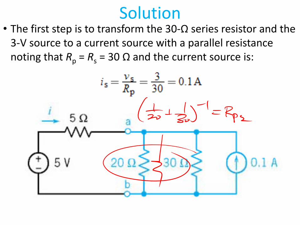
• The first step is to transform the 30‐Ω series resistor and theSolution
The first step is to transform the 30 Ω series resistor and the 3‐V source to a current source with a parallel resistance noting that Rp = Rs = 30 Ω and the current source is:p

• Next, we combine the two parallel resistances to obtainSolution
Next, we combine the two parallel resistances to obtain Rp2 = 12 Ω, as shown below:

• Next, the parallel 12 Ω resistance and the 0.1 A currentSolution
Next, the parallel 12 Ω resistance and the 0.1 A current source can be transformed to a series resistance Rs2 = 12 Ω, with a series voltage source vs as shown below:
• Since source transforms do not alter the currents andSince source transforms do not alter the currents and voltages in the rest of the circuit, current i is found using KVL around the resulting mesh yielding i = 3.8/17 = 0.224 A

Questions?Questions?

• A linear element satisfies superposition when it satisfies theSuperposition
A linear element satisfies superposition when it satisfies the following response and excitation relationship:
Th iti i i l t t th t f i it f li
⇒• The superposition principle states that for a circuit of linear
elements and independent sources we can determine the total response by finding the response to each independenttotal response by finding the response to each independentsource with all other independent sources set to zero, i.e., voltage sources replaced by short circuits and current sources replaced by open circuits, and then sum the individual responses
f d d d d– if a dependent source is present, it is never deactivated and must remain active (unaltered) at all times

Example 5.3‐1: Superposition
• The ammeter current i is the response due to two inputsThe ammeter current im is the response due to two inputs, the voltage source voltage and the current source current; therefore, the superposition principle of tells us we can determine the total response by finding the response to each input acting separately and then adding the responses
htogether

• First set the current source to zero; then the current sourceExample 5.3‐1: Superposition
First set the current source to zero; then the current source appears as an open circuit as shown below
• Current i1 represents the portion of current im that is due to the voltage source acting alone, i.e., a 6 V source appears across a series combination of the 3‐Ω and 6‐Ω resistors; therefore:

• Next, set the voltage source to zero replacing it with a shortExample 5.3‐1: Superposition
Next, set the voltage source to zero replacing it with a short circuit:
• Current i2 represents the portion of current i that is due toCurrent i2 represents the portion of current im that is due to the current source acting alone, i.e., a 2 A source appears to feed into two parallel resistive branches; therefore, we can obtain i2 by the current divider principle as shown:
• The total current is the sum of i1 and i2:
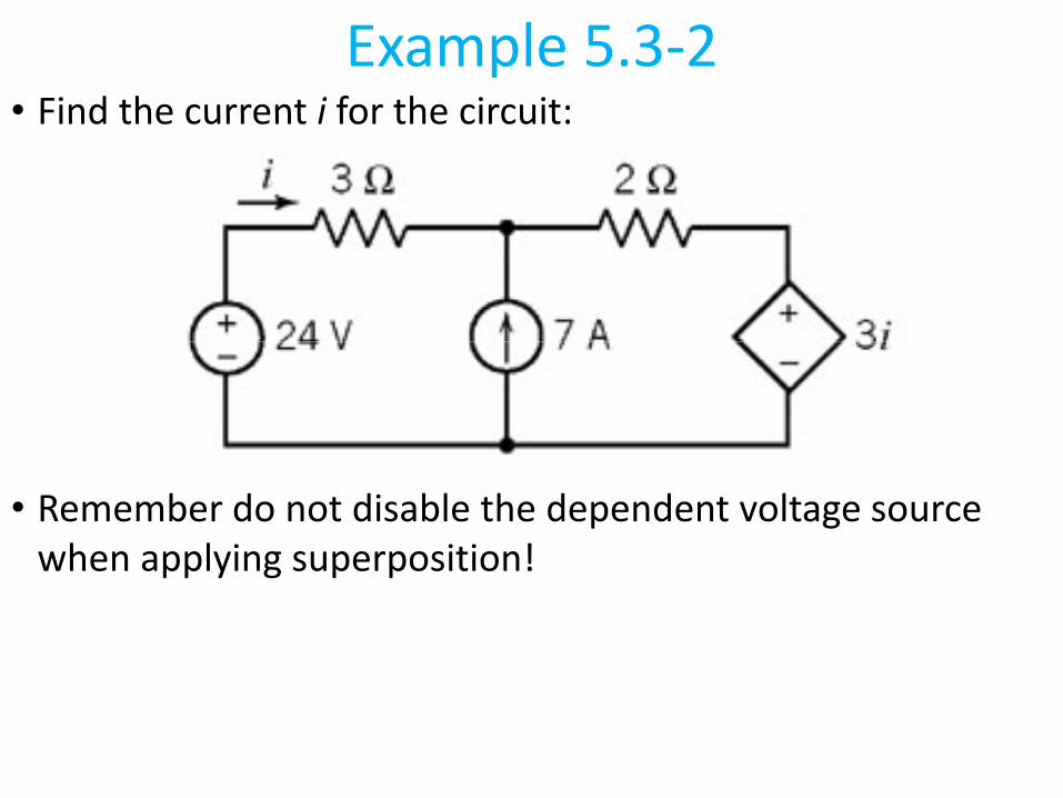
Example 5.3‐2• Find the current i for the circuit:• Find the current i for the circuit:
• Remember do not disable the dependent voltage source when applying superposition!when applying superposition!

Solution• Disabling the current source results in the circuit:Disabling the current source results in the circuit:
A l Ki hh ff' l l h h b i• Apply Kirchhoff's voltage law to the mesh to obtain:

Solution• Disabling the voltage source results in the circuit• Disabling the voltage source results in the circuit:
• First, express the controlling current of the dependent source in terms of the node voltage, va, using Ohm's law:
• Apply Kirchhoff's current law at node a to obtain:Apply Kirchhoff s current law at node a to obtain:

Solution• The current i caused by the two independent sources• The current, i, caused by the two independent sources
acting together is equal to the sum of the currents, i1 and i2, caused by each source acting separately:y g p y

Questions?Questions?

Thévenin's Theorem• A Thévenin equivalent circuit consists of an ideal voltageA Thévenin equivalent circuit consists of an ideal voltage
source in series with a resistor :
≡
• Finding the Thévenin equivalent for circuit A involves three parameters:parameters:
– the open‐circuit voltage, voc– the short‐circuit current, isc– and the Thévenin resistance, Rt
• These parameters are related by:

Thévenin's Theorem• Calculating voc is fairly straight forward:Calculating voc is fairly straight forward:
• For example find v for the circuit below:For example, find voc for the circuit below:
By Voltage Divider:0 5 50 40V
5 20 = = +
0

Thévenin's Theorem• Calculating isc is also straight forward, as shown:Calculating isc is also straight forward, as shown:
Alternately, performa source transform toa source transform, toa Norton equivalent,and use current divider
• For example, find isc for the circuit below:
c By Node Voltage:Since 4v i= ⇒Since 44 50 4 0
5 20
c sc
sc scsc
v ii i i
⇒
−+ + =
5 205Asci⇒ =

Thévenin's Theorem• Calculating Rt, the equivalent resistance of circuit A*, can be t
done in several different ways:
≡oc t
sc t
v vi i
= =
– use the relation: – form circuit A* by disabling independent sources, i.e.,
short voltage and open current sources, then:o “look into the circuit” to determine the resistance (for resistive
circuits without dependent sources)circuits without dependent sources)o apply a test current it = 1A then determine vt from the circuit
and apply the Ohm’s Law relation: t t t tR v i v= = Ω

Thévenin's Theorem• For example, find Rt by “looking into the circuit” below:t
D thi ith ?ocvDoes this agree with ?oc
sci
• If a test source was applied to the modified circuit:5 20 4 8= Ω Ω+ Ω = Ω
pp
( )2 2
By Mesh Currents:5 20 1 0i i+ − =
1A=
24 A54 20(1 0.8)t
i
v
⇒ =
⇒ = + −1A= ( ) 8V
8
t
t tR v=
∴ = = Ω

Thévenin's Theorem• The Thévenin equivalent circuit is therefore given by:

• Find the Thévenin equivalent circuit for the circuit below:Example 5.4‐2: Thévenin Equivalent Circuit
• One approach is to find the open‐circuit voltage and the i i ' Thé i i l i R hcircuit's Thévenin equivalent resistance Rt, as shown:
( )10 40 48 4 12
= +
8 4 12= + =

• To determine the open‐circuit voltage at terminals a–b Example 5.4‐2: Thévenin Equivalent Circuit
observe that no current flows through the 4‐Ω resistor, therefore, the open‐circuit voltage is identical to the voltage across the 40 Ω resistor v :across the 40‐Ω resistor, vc:
8Voc cv v= = −
• Using the bottom node as the reference we write KCL at• Using the bottom node as the reference, we write KCL at node c to obtain:
⇒⇒

Solution• Therefore, the Thévenin equivalent circuit is given by:

Example 5.4‐4: Thévenin Equivalent Circuits with Dependent Sources
• Find the Thévenin equivalent circuit for the circuit below:p
• To determine the open‐circuit voltage vab = voc note that the t /4 id i t t hcurrent source vab/4 provides is common to two meshes;
therefore, we create a supermesh that includes vab and write one KVL equation around the supermesh:write one KVL equation around the supermesh:
⇒

Example 5.4‐4: Thévenin Equivalent Circuits with Dependent Sources
• To find the short‐circuit current, we establish a short circuit across a–b, as shown below:
p
Si 0 th t t i th KVL• Since vab = 0, the current source current is zero; thus KVL around the periphery of the supermesh gives:
⇒

Solution• Therefore, the
• With the Thévenin equivalent circuit:
10Ω
10V
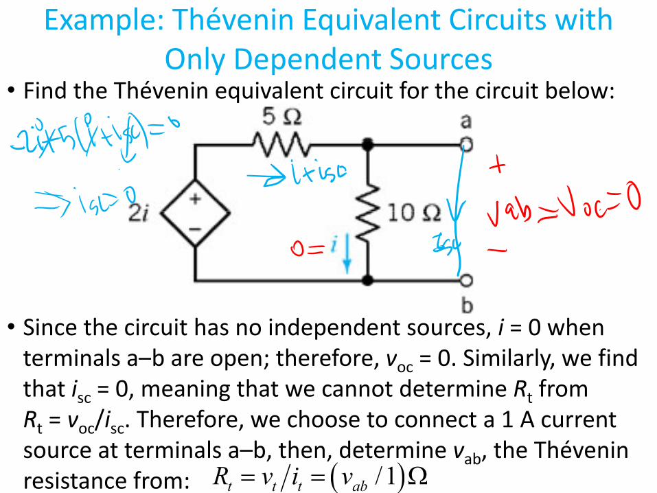
Example: Thévenin Equivalent Circuits with Only Dependent Sources
• Find the Thévenin equivalent circuit for the circuit below:y p
• Since the circuit has no independent sources, i = 0 when t i l b th f 0 Si il l fi dterminals a–b are open; therefore, voc = 0. Similarly, we find that isc = 0, meaning that we cannot determine Rt from R = v /i Therefore we choose to connect a 1 A currentRt = voc/isc. Therefore, we choose to connect a 1 A current source at terminals a–b, then, determine vab, the Théveninresistance from: ( )/1t t t abR v i v= = Ω

Example: Thévenin Equivalent Circuits with Only Dependent Sources
• Applying the 1 A test source to the circuit below:y p
• Writing KCL and KVL at a with b as the reference, we obtain: and
⇒ ⇒

Solution• Therefore, the Thévenin equivalent circuit is given by:

Example: Experimental Determination of a Thévenin Equivalent Circuit
• A laboratory procedure for determining the Théveninequivalent of a black box circuit is to measure i and v for two
q
or more values of vs and a fixed value of R, as shown below:
• Replace the test circuit with its Thévenin equivalent, obtaining: g

Example: Experimental Determination of a Thévenin Equivalent Circuit q
• The procedure is to measure v and i for a fixed R and several• The procedure is to measure v and i for a fixed R and several values of vs, e.g., let R = 10 Ω and consider the two measurement results (solving using MATLAB): ( g g )
⇒∴

Questions?Questions?

Norton's Theorem & Equivalent Circuits
≡≡n tR R=
• Norton's theorem may be stated as follows: divide a linear circuit into two subcircuits, A and B; consider circuit A and determine the short‐circuit current isc at its terminals– the Norton Equivalent circuit is a current source isc in
parallel with resistance Rn, the resistance looking into circuit A with independent sources deactivated, i.e., A*
– note, if either A or B contains a dependent source its controlling variable must be in the same subcircuit

Example 5.5‐1: Norton Equivalent Circuit• Note, the Norton equivalent circuit is simply the source
transformed Thévenin equivalent, as illustrated below:
• Disable the voltage source by replacing with a short circuit, g y p g ,then looking into the circuit from terminal a to b, we obtain:
( ) 12k 6k8k 4k 6k 4kR R Ω⋅ Ω= = Ω+ Ω Ω = = Ω( )8k 4k 6k 4k
12k +6kn tR R= = Ω+ Ω Ω = = ΩΩ Ω

Example 5.5‐1: Norton Equivalent Circuit• To determine isc, we short‐circuit the output terminals with sc
the voltage source activated as shown below:
• Writing KCL at node a we have:
⇒
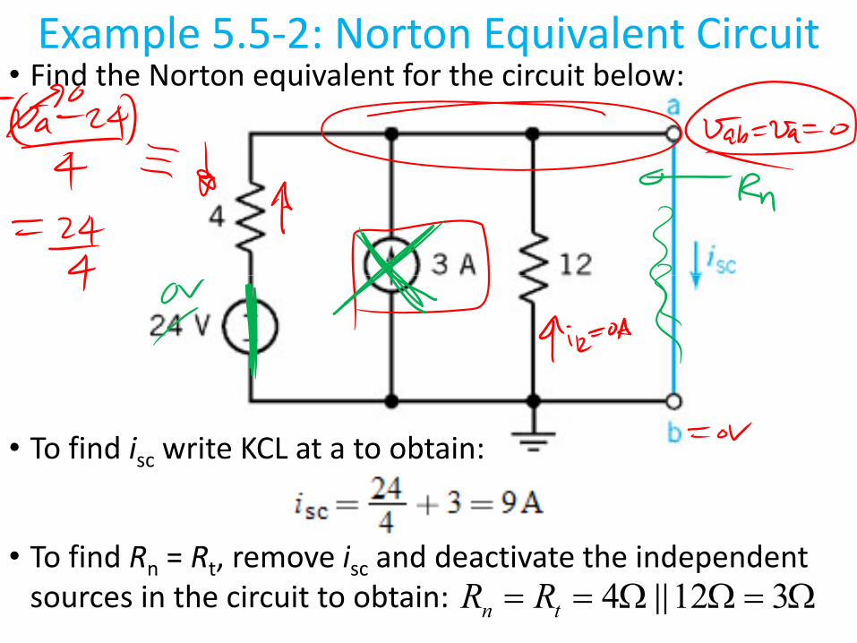
Example 5.5‐2: Norton Equivalent Circuit• Find the Norton equivalent for the circuit below:
• To find isc write KCL at a to obtain:sc
T fi d R R i d d ti t th i d d t• To find Rn = Rt, remove isc and deactivate the independent sources in the circuit to obtain: 4 12 3n tR R= = Ω Ω = Ω

Example 5.5‐3: Norton Equivalent Circuits and Dependent Sourcesand Dependent Sources
• Find the Norton equivalent to the left of terminals a–b for the circuit below:
• Determine the short‐circuit current isc noting that vab = 0 sc g abwhen the terminals are short‐circuited:
• Therefore, for the right‐hand portion of the circuit:

Example 5.5‐3: Norton Equivalent Circuits and Dependent Sourcesand Dependent Sources
• To determine Rn = Rt, remove isc and deactivate the independent sources in the circuit, to find voc = vab:
• Writing the mesh current equation where i is the current in g qthe left‐hand mesh:
• Thus, for the right‐hand mesh:, g
⇒⇒ ⇒

Example 5.5‐3: Norton Equivalent Circuits and Dependent Sourcesand Dependent Sources
• Therefore, Rn = Rt, is obtained as:
• So the Norton equivalent circuit is given by:
• Note, the direction of isc is downward, which is consistent with the signs of isc and voc = vab compared to the references

Questions?Questions?
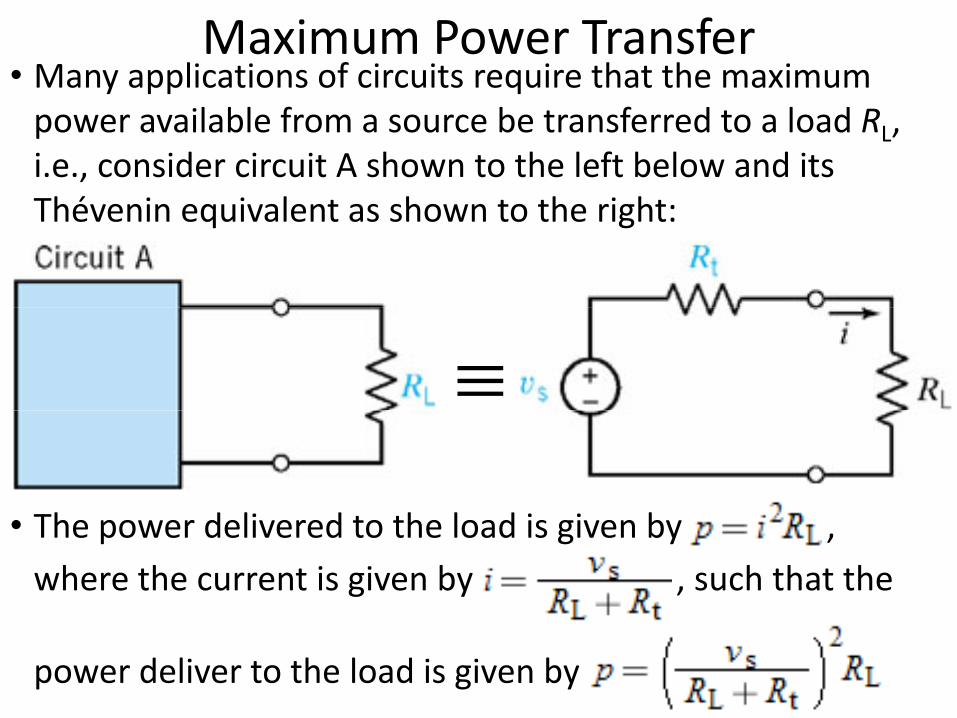
Maximum Power Transfer• Many applications of circuits require that the maximum
power available from a source be transferred to a load RL, i.e., consider circuit A shown to the left below and its Thévenin equivalent as shown to the right:Thévenin equivalent as shown to the right:
≡h d l d h l d b• The power delivered to the load is given by ,
where the current is given by , such that the
power deliver to the load is given by

Maximum Power Transfer• Assuming that vs and Rt are fixed for a given source, the
maximum power is a function of RL
• To find the value of RL that maximizes the power, we use the d ff l l l f d h h d d /ddifferential calculus to find where the derivative dp/dRLequals zero; taking the derivative, we obtain:
Th d i i i h 0 ( i i l l i )• The derivative is zero when vs = 0 (a trivial solution) or:
f h h l d⇒
– to confirm that this solution corresponds to a maximum, it should be shown that d2p/d RL
2 < 0th f th i i t f d t th l d– therefore; the maximum power is transferred to the load when RL is equal to the Thévenin equivalent resistance Rt

Maximum Power Transfer• Note, this solution can be verified using MATLAB as shown:
>> syms Rt, RL>> solve('(Rt+RL)^2‐2*(Rt+RL)*RL=0',RL)ans =ans =
Rt‐Rt % Reject this solution since Rt can not be < 0
• Substituting RL = Rt into the power expression yields: Rt % Reject this solution since Rt can not be 0
where v for the Thévenin source voltage i is the Nortonwhere vs for the Thévenin source voltage, is is the Norton source current and Rt is the Thévenin/Norton equivalent resistance
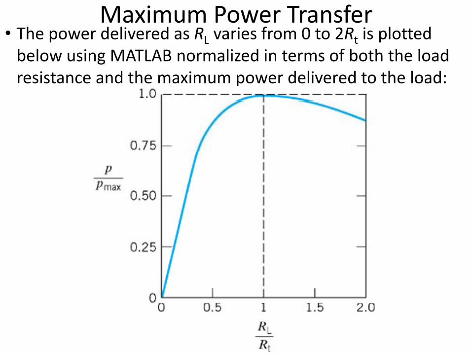
Maximum Power Transfer• The power delivered as RL varies from 0 to 2Rt is plotted
b l i MATLAB li d i t f b th th l dbelow using MATLAB normalized in terms of both the load resistance and the maximum power delivered to the load:

Example 5.6‐2: Maximum Power Transfer• Find load RL that results in pmax delivered for the circuit:
• We can compute Rt from Rt = voc/isc (Method 2 of text)
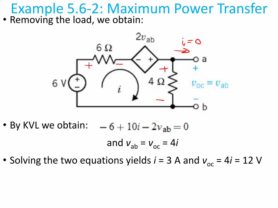
Example 5.6‐2: Maximum Power Transfer• Removing the load, we obtain:
• By KVL we obtain:
and vab = voc = 4iab oc
• Solving the two equations yields i = 3 A and voc = 4i = 12 V

Example 5.6‐2: Maximum Power Transfer• Shorting the load, we obtain:
• Since the 4‐Ω resistor is short‐circuited, it can be ignored; thus KVL yields:
isc = 1 A
• Given voc = 4i = 12 V; therefore, Rt = RL = voc/isc = 12 Ω and ⇒
oc t L oc sc

Example 5.6‐2: Maximum Power Transfer• The Thévenin equivalent circuit is shown below with the
load resistor for maximum power delivered reconnected:

Questions?Questions?

Example 5.6‐2: Verification I• Verify Rt from Rt = vt/it (Method 3 of text):

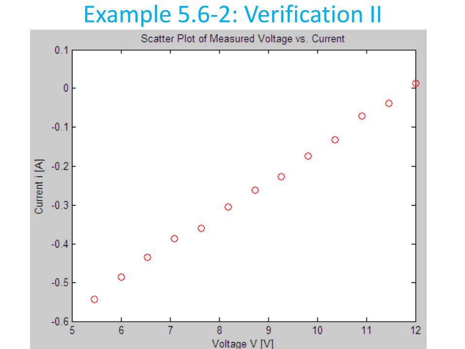
Example 5.6‐2: Verification II• Verify Rt using a simulated experimental measurements:
• Since we will simulate the measurements i e using• Since we will simulate the measurements, i.e., using MATLAB, we need to analyze the circuit, as shown:

Example 5.6‐2: Verification II• We can compute Rt experimentally from:
Si l t th t f f d fi d• Simulate the measurements for a range of vs and a fixed value of R, as shown in the MATLAB script Ex_5_6_2.m:clearclearVs=(0:12)';R=10;% Note: Vab=V% U i h t th i it bt i% Using mesh currents on the circuit, we obtain:V=24*(Vs+R)/(2*R+24)i=((Vs‐V)/R)+0.025*rand(size((0:12)'))% Note, a random component added to the current for realismplot(V,i,'ro')xlabel('Voltage V [V]')xlabel( Voltage V [V] )ylabel('Current i [A]')title('Scatter Plot of Measured Voltage vs. Current')% D fi th t [V Rt]’ h th t V [ ( i (i)) i]* A*% Define the vector x = [Voc;Rt]’ such that V = [ones(size(i));i]*x =A*xA = [ones(size(i)),i]x = A\V
Example 5.6‐2: Verification II

Example 5.6‐2: Verification II• MATLAB results:% Simulated measurementsV =
5 4545
% x = [Voc;Rt]’x = A\V =
11 8712i =
0 5441
% A = [ones(size(i));i]A =
1 0000 0 54415.45456.00006.5455
11.871212.0026
This agrees
‐0.5441‐0.4867‐0.4351
1.0000 ‐0.54411.0000 ‐0.48671.0000 ‐0.4351
7.09097.63648 1818
with our prior results!
‐0.3857‐0.3604‐0 3040
1.0000 ‐0.38571.0000 ‐0.36041 0000 ‐0 30408.1818
8.72739.27279 8182
0.3040‐0.2610‐0.22700 1734
1.0000 0.30401.0000 ‐0.26101.0000 ‐0.22701 0000 0 17349.8182
10.363610.9091
‐0.1734‐0.1323‐0.0711
1.0000 ‐0.17341.0000 ‐0.13231.0000 ‐0.0711
11.454512.0000
‐0.03770.0132
1.0000 ‐0.03771.0000 0.0132


