ESDC DocumentationRelease 3.0

Brockmann Consult GmbHMPI Biogeochemistry Jena

Stockholm Resilience Centre

May 14, 2018

Contents

1 Introduction 31.1 Motivation . . . . . . . . . . . . . . . . . . . . . . . . . . . . . . . . . . . . . . . . . . . . . . . . 31.2 ESDC Project . . . . . . . . . . . . . . . . . . . . . . . . . . . . . . . . . . . . . . . . . . . . . . . 41.3 Purpose . . . . . . . . . . . . . . . . . . . . . . . . . . . . . . . . . . . . . . . . . . . . . . . . . . 41.4 Scope . . . . . . . . . . . . . . . . . . . . . . . . . . . . . . . . . . . . . . . . . . . . . . . . . . . 41.5 References . . . . . . . . . . . . . . . . . . . . . . . . . . . . . . . . . . . . . . . . . . . . . . . . 41.6 Peer-reviewed Publications . . . . . . . . . . . . . . . . . . . . . . . . . . . . . . . . . . . . . . . 51.7 Terms and Abbreviations . . . . . . . . . . . . . . . . . . . . . . . . . . . . . . . . . . . . . . . . . 51.8 Data Policy . . . . . . . . . . . . . . . . . . . . . . . . . . . . . . . . . . . . . . . . . . . . . . . . 51.9 Legal information . . . . . . . . . . . . . . . . . . . . . . . . . . . . . . . . . . . . . . . . . . . . 6

2 ESDC Description 72.1 Macro Structure . . . . . . . . . . . . . . . . . . . . . . . . . . . . . . . . . . . . . . . . . . . . . 72.2 Spatial and Temporal Coverage . . . . . . . . . . . . . . . . . . . . . . . . . . . . . . . . . . . . . 72.3 Format and Structure . . . . . . . . . . . . . . . . . . . . . . . . . . . . . . . . . . . . . . . . . . . 82.4 Processing Applied . . . . . . . . . . . . . . . . . . . . . . . . . . . . . . . . . . . . . . . . . . . . 92.5 Cube Data Variables . . . . . . . . . . . . . . . . . . . . . . . . . . . . . . . . . . . . . . . . . . . 11

3 ESDC Access 153.1 Download ESDC Data . . . . . . . . . . . . . . . . . . . . . . . . . . . . . . . . . . . . . . . . . . 153.2 OPeNDAP and WCS Services . . . . . . . . . . . . . . . . . . . . . . . . . . . . . . . . . . . . . . 153.3 E-Laboratory . . . . . . . . . . . . . . . . . . . . . . . . . . . . . . . . . . . . . . . . . . . . . . . 163.4 Using Python . . . . . . . . . . . . . . . . . . . . . . . . . . . . . . . . . . . . . . . . . . . . . . . 163.5 Using Julia . . . . . . . . . . . . . . . . . . . . . . . . . . . . . . . . . . . . . . . . . . . . . . . . 193.6 Data Analysis . . . . . . . . . . . . . . . . . . . . . . . . . . . . . . . . . . . . . . . . . . . . . . . 20

4 ESDC Generation 214.1 Command-Line Tool . . . . . . . . . . . . . . . . . . . . . . . . . . . . . . . . . . . . . . . . . . . 214.2 Writing a new Provider . . . . . . . . . . . . . . . . . . . . . . . . . . . . . . . . . . . . . . . . . . 224.3 Sharing a Provider . . . . . . . . . . . . . . . . . . . . . . . . . . . . . . . . . . . . . . . . . . . . 234.4 Python Cube API Reference . . . . . . . . . . . . . . . . . . . . . . . . . . . . . . . . . . . . . . . 23

5 DAT for Julia 275.1 Overview . . . . . . . . . . . . . . . . . . . . . . . . . . . . . . . . . . . . . . . . . . . . . . . . . 275.2 Use Cases and Examples . . . . . . . . . . . . . . . . . . . . . . . . . . . . . . . . . . . . . . . . . 28

6 DAT for Python 29

i

6.1 Overview . . . . . . . . . . . . . . . . . . . . . . . . . . . . . . . . . . . . . . . . . . . . . . . . . 296.2 Use Cases and Examples . . . . . . . . . . . . . . . . . . . . . . . . . . . . . . . . . . . . . . . . . 306.3 Python API Reference . . . . . . . . . . . . . . . . . . . . . . . . . . . . . . . . . . . . . . . . . . 35

7 Collaboration 377.1 Code Repository . . . . . . . . . . . . . . . . . . . . . . . . . . . . . . . . . . . . . . . . . . . . . 377.2 Website & Forum . . . . . . . . . . . . . . . . . . . . . . . . . . . . . . . . . . . . . . . . . . . . . 37

8 Indices and Tables 39

ii

ESDC Documentation, Release 3.0

The Earth System Data Cube (ESDC) is a multi-variate data set of essential Earth System variables on a common gridand sharing a common data model. The ESDC also comprises a Data Analytics Toolkit for Julia, Python, and R tofacilitate the exploitation data set and an E-Laboratory, which provides a computing environment to access, analyseand visualize the data set.

Our goal is to foster a holistic understanding of the Earth System by simplifying the simultaneous and consistentanalysis of big and freely available data sets of geopyhsical variables.

Contents 1

ESDC Documentation, Release 3.0

2 Contents

CHAPTER 1

Introduction

1.1 Motivation

Earth observations (EOs) are usually produced and treated as 3-dimensional singular data cubes, i.e. for each longitudeu {1, . . . , Lon}, each latitude v {1, . . . , Lat}, and each time step t {1,. . . ,T} an observation X = {x(u,v,t)} R is defined.The challenge is, however, to take advantage of the numerous EO streams and to explore them simultaneously. Hence,the idea is to concatenate data streams such that we obtain a 4-dimensional data cube of the form x(u,v,t,k) where k{1, . . . , N} denotes the index of the data stream. The focus of this project is therefore on learning how to efficientlyand reliably create, curate, and explore a 4-dimensional Earth System Data Cube (ESDC). If feasible, the includeddata-sets contain uncertainty information. Limitations associated with the transformation from source format into theESDC format are explained in the description of the data sets. The ESDC does not exhibit spatial or temporal gaps,since gaps in the source data are filled during ingestion into the ESDC. While all observational values are conserved,gaps are filled with synthetic data, i.e. with data that is created by an adequate gap-filling algorithm. Proper data flagsensure an unambiguous distinction between observational and synthetic data values.

Depending on the specific question, the user can extract different types of data subsets from the Earth System DataCube (ESDC) for further processing and analysis with specialized methods from the Data Analytics Toolkit. Forexample,

• investigating the data cube at a single geographic location, the user obtains multivariate time series for eachlongitude-latitude pair. These time series can be investigated using established methods of multivariate timeseries analysis, and afterwards the results can be merged onto a global grid again.

• Assessing the data-cube at single time stamps results in synoptic geospatial maps, whose properties can beinvestigated with geostatistical methods.

• It is also possible to perform univariate spatiotemporal analyses on single variables extracted from the DataCube.

• The main objective is, however, to develop multivariate spatiotemporal analyses by utilizing the entire 4DESDC. Following this avenue unravels the full potential of the ESDC and may provide a holistic view on theentire Earth System.

The ESDC allows for all these approaches, because all variables are available on a common spatiotemporal grid,which greatly reduces the pre-processing efforts typically required to establish consistency among data from different

3

ESDC Documentation, Release 3.0

sources.

1.2 ESDC Project

The steadily growing Earth Observation archives are currently mostly investigated by means of disciplinary ap-proaches. It would be, however, desirable to adopt a more holistic approach in understanding land-atmosphere in-teractions and the role of humans in the earth system. The potential of a simultaneous exploration of multiple EO datastreams has so far been widely neglected in the scientific community. The Earth System Data Cube project (ESDC,formerly CAB-LAB) aims at filling this gap by providing a virtual laboratory that facilitates the co-exploration ofmultiple EOs for a better understanding of land ecosystem trajectories.

The idea is to build on the existing data-sets and to offer novel tools and technical methods to detect dependenciesin the coupled human-nature system. ESDC’s central service to the scientific community will be a Biosphere Atmo-sphere Virtual Laboratory (BAVL), which comprises a Data Cube populated with a wide range of EOs and convenientmethods to access and analyze this data remotely by means of the Jupiter framework. Moreover, the project aims atadvancing the scientific analysis capacities by developing data-driven exploration strategies that identify and attributemajor changes in the biosphere-atmosphere system. Ultimately, ESDC will develop a set of indices characterizing themajor relevant Biosphere-Atmosphere System Trajectories, BASTs. The project partners, Max-Planck-Institute forBiogeochemistry, Brockmann Consult GmbH, and Stockholm Resilience Center are financed by the European SpaceAgency (ESA) for three years (2015 to 2017) to develop the software for ESDC, to collect and analyze the EO data,and to disseminate the idea of the project and its preliminary results.

1.3 Purpose

This Product Handbook is a living document that is under active development just as the ESDC project itself. Itspurpose is to facilitate the usage of the BAVL and primarily targets scientists from various disciplines with a goodcommand of one of the supported high-level programming languages (Python, Julia, and R), a solid background in theanalysis of large data-sets, and a sound understanding of the Earth System. The focus of this document is thereforeclearly on the description of the data and on the methods to access and manipulate the data.

In the final version, it is meant to be a self-contained documentation that enables the user to independently reap the fullpotential of the Earth System Data Cube (ESDC). Developers may find a visit of the project’s git-hub pages worthwile.

1.4 Scope

The Product Handbook gives a general overview of the ESCD’s structure and provide some examples to illustratepotential uses of the system . The main part is considered with a detailed technical description of the ESDC , which isaccompanied by the full specification of the API. Finally, all data-sets included in the ESDC are listed and describedin the annex of the Product Handbook.

1.5 References

1. ESDC webpage: http://www.earthsystemdatacube.net

2. CAB-LAB’s github repository: https://github.com/CAB-LAB

3. E-Laboratory: https://cablab.earthsystemdatacube.net

4 Chapter 1. Introduction

ESDC Documentation, Release 3.0

1.6 Peer-reviewed Publications

Sippel, S., Lange, H., Mahecha, M. D., Hauhs, M., Bodesheim, P., Kaminski, T., Gans, F. & Rosso, O.A. (2016)Diagnosing the Dynamics of Observed and Simulated Ecosystem Gross Primary Productivity with Time Causal Infor-mation Theory Quantifiers. PLoS ONE, accepted. doi:10.1371/journal.pone.0164960.

Sippel, S., Zscheischler, J., Heimann, M., Otto, F. E. L., Peters, J., & Mahecha, M. D. (2015), Quantifying changesin climate variability and extremes: Pitfalls and their overcoming, Geophysical Research Letters, 42(22), 9990–9998.doi:10.1002/2015GL066307.

Sippel, S., Zscheischler, J., Heimann, M., Lange, H., Mahecha, M. D., van Oldenborgh, G. J., Otto, F. E. L. &Reichstein, M. (2016) Have precipitation extremes and annual totals been increasing in the world’s dry regions overthe last 60 years? Hydrology and Earth System Sciences Discussions. doi:10.5194/hess-2016-452.

Flach, M., Gans, F., Brenning, A., Denzler, J., Reichstein, M., Rodner, E., Bathiany, S., Bodesheim, P., Guanche, Y.,Sippel, S., and Mahecha, M.D. Multivariate Anomaly Detection for Earth Observations: A Comparison of Algorithmsand Feature Extraction Techniques. Earth System Dynamics – Discussions, doi:10.5194/esd-2016-51.

1.7 Terms and Abbreviations

Term DescriptionBAST Biosphere-Atmosphere System TrajectoryBAVL Biosphere Atmosphere Virtual LaboratoryCAB-LAB Coupled Atmosphere Biosphere virtual LABoratoryDAT Data Analytics ToolkitESDC Earth System Data CubeEO Earth ObservationsESA European Space AgencyGrid The Data Cube’s layout given by its spatial and temporal resolution and its variables.Image An 2D data cube subset with dimension (lat, lon)

1.8 Data Policy

The ESDC team processes and distributes the data in the ESDC in good faith, but makes no warranty, expressed orimplied, nor assumes any legal liability or responsibility for any purpose for which the data are used. In particular, theESDC team does not claim ownership of the data distributed through the ESDC nor does it alter the data policy of thedata owner. Therefore, the user is referred to the data owner for specific questions of data use. References and moredetails of the data sets are listed in the annex of the Product Handbook.

The CAB-LAB team is thankful to have received permissions for re-distribution of all data contained in the ESDCfrom the respective data owners.

Note: Please cite the ESDC as:

The ESDC developer team (2016). The Earth System Data Cube (Version 0.1), available at: https://github.com/CAB-LAB.

1.6. Peer-reviewed Publications 5

ESDC Documentation, Release 3.0

1.9 Legal information

The Earth System Data Cube consists of a variety of source data sets from different providers, the Data Cube software,which transforms all data to the common Data Cube format and allows for convenient data access, and the DataAnalytics Toolkit, which provides methods for scientific analysis.

The Data Cube software and the Data Analytics Toolkit are free software: you can redistribute it and/or modify itunder the terms of the GNU General Public License as published by the Free Software Foundation, either version 3 ofthe License, or (at your option) any later version.

This program is distributed in the hope that it will be useful, but WITHOUT ANY WARRANTY; without even theimplied warranty of MERCHANTABILITY or FITNESS FOR A PARTICULAR PURPOSE. See the GNU GeneralPublic License for more details.

You should have received a copy of the GNU General Public License along with this program. If not, see http://www.gnu.org/licenses/.

Copyright (C) 2016 The ESDC developer team.

6 Chapter 1. Introduction

CHAPTER 2

ESDC Description

2.1 Macro Structure

The data is organised in the described 4-dimensional form x(u,v,t,k), but additionally each data stream k is assigned toone of the subsystems of interest:

• Land surface

• Atmospheric forcing

• Socio-economic data

2.2 Spatial and Temporal Coverage

The fine grid of the ESDC has a spatial resolution of 0.083° (5”), which is properly nested within a coarse grid of0.25° (15”). Hence, the ESDC is available in two versions

• High resolution version: 0.083° (5”) spatial resolution,

• Low resolution version: 0.25° (15”) spatial resolution.

While the latter contains all variables, the former only comprises those variables that are natively available at thisresolution. The high-resolution data are nested on the low-resolution data set such that one can analyse these intandem. In particular data from the socio-economic subsystem are often organised according to administrative units,typically national states, rather than on regular grids. These data are dispersed to the coarse grid by means of a nationalstate mask, which is created by assigning a national state property to each grid point.

The temporal resolution is 8 days.

The time span currently covered is 2001-2011. We are dedicated to expand this period on both ends, but to preservethe ESDC’s characteristics, a reasonable coverage of data streams is required.

7

ESDC Documentation, Release 3.0

2.3 Format and Structure

The binary data format for the Earth System Data Cube (ESDC) in the CAB-LAB project is netCDF 4 classic, wherethe term classic stands for an underlying HDF-5 format accessed by a netCDF 4 API.

The netCDF file’s content and structure follows the CF-conventions. That is, there are are always at least threedimensions defined

1. lon - Always the inner and therefore fastest varying dimension. Defines the raster width of spatial images.

2. lat - Always the second dimension. Defines the raster height of spatial images.

3. time - Time dimension.

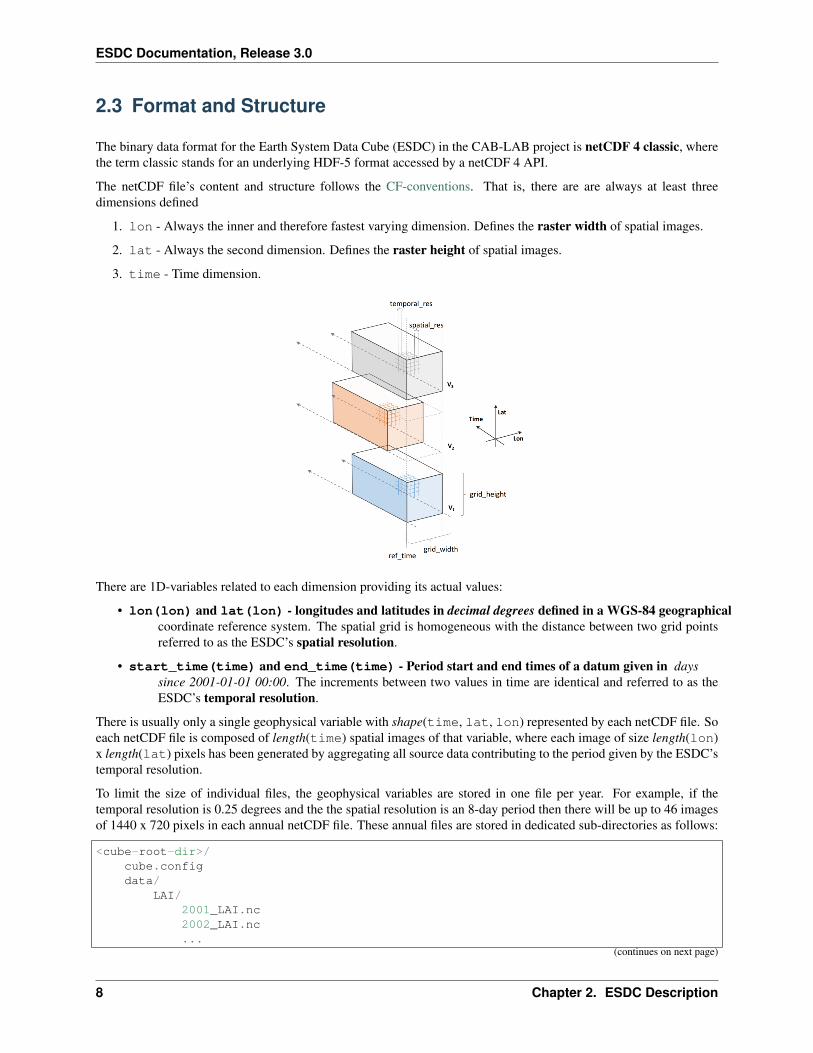
There are 1D-variables related to each dimension providing its actual values:

• lon(lon) and lat(lon) - longitudes and latitudes in decimal degrees defined in a WGS-84 geographicalcoordinate reference system. The spatial grid is homogeneous with the distance between two grid pointsreferred to as the ESDC’s spatial resolution.

• start_time(time) and end_time(time) - Period start and end times of a datum given in dayssince 2001-01-01 00:00. The increments between two values in time are identical and referred to as theESDC’s temporal resolution.

There is usually only a single geophysical variable with shape(time, lat, lon) represented by each netCDF file. Soeach netCDF file is composed of length(time) spatial images of that variable, where each image of size length(lon)x length(lat) pixels has been generated by aggregating all source data contributing to the period given by the ESDC’stemporal resolution.

To limit the size of individual files, the geophysical variables are stored in one file per year. For example, if thetemporal resolution is 0.25 degrees and the the spatial resolution is an 8-day period then there will be up to 46 imagesof 1440 x 720 pixels in each annual netCDF file. These annual files are stored in dedicated sub-directories as follows:

<cube-root-dir>/cube.configdata/

LAI/2001_LAI.nc2002_LAI.nc...

(continues on next page)

8 Chapter 2. ESDC Description

ESDC Documentation, Release 3.0

(continued from previous page)

2011_LAI.ncOzone/

2001_Ozone.nc2002_Ozone.nc...2011_Ozone.nc

...

The names of the geophysical variable in a netCDF file must match the name of the corresponding sub-directory andthe file name.

The text file cube.config contains a Data Cube’s static configuration such as its temporal and spatial resolution.Also the spatial coverage is constant, that is, all spatial images are of the same size. Where actual data is missing,fill values are inserted to expand a data set to the dimensions of the Data Cube. The fill values in the Data Cube areidentical to the ones used in the Data Cube’s sources. The same holds for the data types. While all images for all timeperiods have the same size, the temporal coverage for a given variable may vary. Missing spatial images for a giventime period are treated as images with all pixels set to a fill value.

The following table contains all possible configuration parameters:

Parameter Default Value Descriptiontemporal_res 8 The constant temporal resolution given as integer days.calendar 'gregorian' Defines the Data Cube’s time units.ref_time datetime(2001, 1,

1)The Data Cube’s time unit is days since a reference date/time.

start_time datetime(2001, 1,1)

The start date/time of contributing source data.

end_time datetime(2011, 1,1)

The end date/time of contributing source data.

spatial_res 0.25 The constant spatial resolution given in decimal degrees.grid_x0 0 The spatial grid’s X-offset.grid_y0 0 The spatial grid’s Y-offset.grid_width 1440 The spatial grid’s width. Must always be 360 /

spatial_res.grid_height 720 The spatial grid’s height. Must always be 180 /

spatial_res.variables None The variables contained in the Data Cube.file_format 'NETCDF4_CLASSIC' The target binary file format.compression False Whether or not the target binary files should be compressed.model_version '0.1' The version of the Data Cube model and configuration.

2.4 Processing Applied

The Data Cube is generated by the cube-cli tool. This tools creates a Data Cube for a given configuration and canbe used to subsequently add variables, one by one, to the Data Cube. Each variable is read from its specific data sourceand transformed in time and space to comply to the specification defined by the target Data Cube’s configuration.

The general approach is as follows: For each variable and a given Data Cube time period: * Read the variable’sdata from all contributing sources that have an overlap with the target period; * Perform temporal aggregation of allcontributing spatial images in the original spatial resolution; * Perform spatial upsampling or downsampling of theimage aggregated in time; * Mask the resulting upsampled/downsampled image by the common land-sea mask; *Insert the final image for the variable and target time period into the Data Cube.

2.4. Processing Applied 9

ESDC Documentation, Release 3.0

The following sections describe each method used in more detail.

2.4.1 Gap-Filling Approach

The current version (version 0.1, Feb 2016) of the ESDC does not explicitly fill gaps. However, some gap-fillingoccurs during temporal aggregation as described below. The CAB-LAB team may provide gap-filled ESDC versionsat a later point in time of the project. Gap-filling is part of the Data Analytics Toolkit and is thus not tackled duringData Cube generation to retain the information on the original data coverage as much as possible.

For future Data Cube versions per-variable gap-filling strategies may be applied. Also, only a spatio-temporal regionof interest may be gap-filled while cells outside this region may be filled by global default values. An instructiveexample of such an approach would be the gap-filling of a leaf area index (LAI) data set, which only takes place inmid-latitudes while gaps in high-latitudess are filled with zeros.

2.4.2 Temporal Resampling

Temporal resampling starts on the 1st January of every year so that all the i-th spatial images in the ESDC refer to thesame time of the year, namely starting i x temporal resolution. Source data is collected for every resulting ESDC targetperiod. If there is more than one contribution in time, then each contribution is weighted according to the temporaloverlap with the target period. Finally, target pixel values are computed by averaging all weighted values in time notmasked by a fill value. By doing so, some temporal gaps are filled implicitly.

2.4.3 Spatial Resampling

Spatial resampling occurs after temporal resampling only if the ESDC’s spatial resolution differs from the data sourceresolution.

If the ESDC’s spatial resolution is higher than the data source’s spatial resolution, source images are upsampled byrescaling hereby duplicating original values, but not performing any spatial interpolation.

If the ESDC’s spatial resolution is lower than the data source’s spatial resolution, source images are downsampledby aggregation hereby performing a weighted spatial averaging taking into account missing values. If there is not aninteger factor between the source and the Data Cube resolution, weights will be found according to the spatial overlapof source and target cells.

10 Chapter 2. ESDC Description

ESDC Documentation, Release 3.0

2.4.4 Land-Water Masking

After spatial resampling, a land-water mask is applied to individual variables depending on whether a variable isdefined for water surfaces only, land surfaces only, or both. A common land-water mask is used for all variables for agiven spatial resolution. Masked values are indicated by fill values.

2.4.5 Constraints and Limitations

The ESDC approach of transforming all variables onto a common grid greatly facilitates handling and joint analysisof data sets that originally had different characteristics and were generated under different assumptions. Regridding,gap-filling, and averaging, however, may alter the information contained in the original data considerably.

The main idea of the ESDC is to provide a consistent and synoptic characterisation of the Earth System at given timesteps to promote global analyses. Therefore, conducting small-scale, high frequency studies that are potentially highlysensible to individual artifacts introduced by data transformation is not encouraged. The cautious expert user mayhence carefully check phenomena close to the Land-Sea mask or in data sparse regions of the original data. If indoubt, suspicious patterns in the ESDC or unexpected analytical results should be verified with the source data in thenative resolution. We try here as much as possible to conserve the characteristics of the original data, while facilitatingdata handling and analysis by transformation.

This is a difficult balance to strike that at times involves inconvenient trade-offs. We thus embrace transparency andreproducibility to enable the informed user to evaluate the validity and consistency of the processed data and strive tooffer options for data transformation wherever possible.

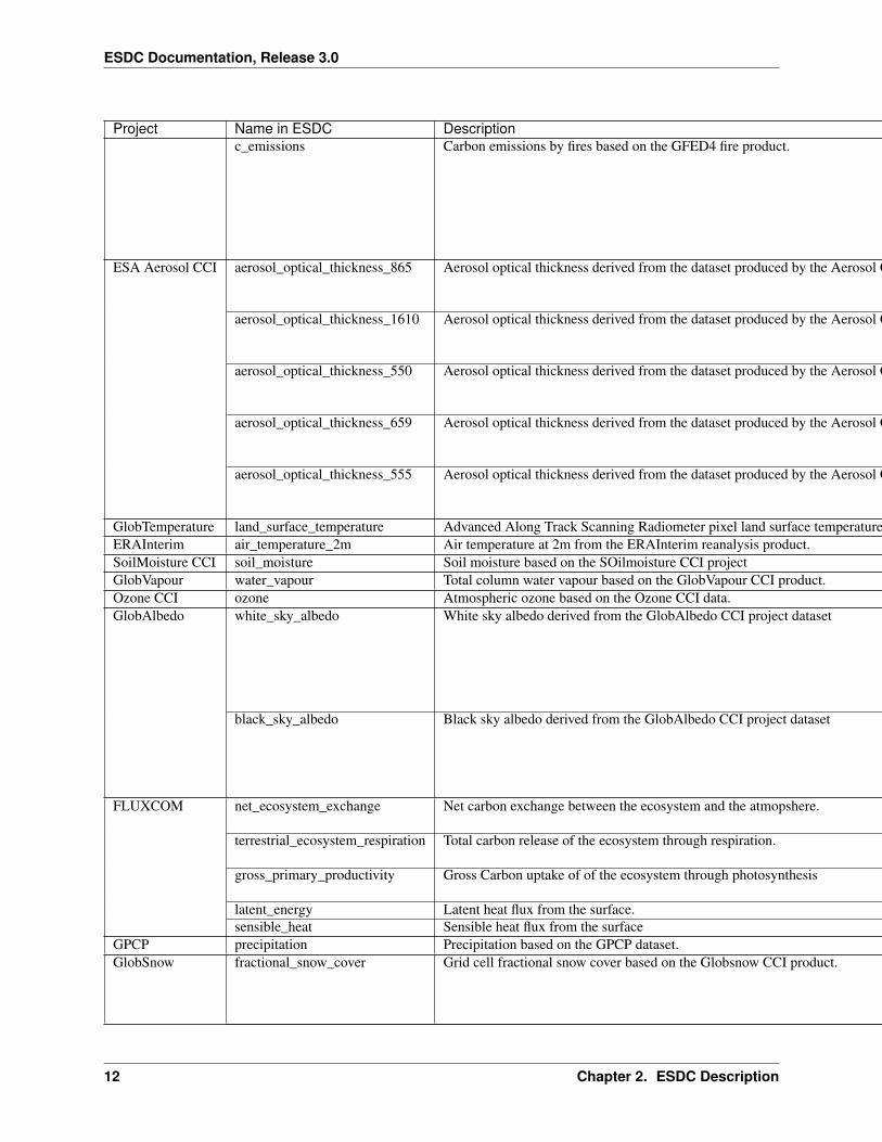
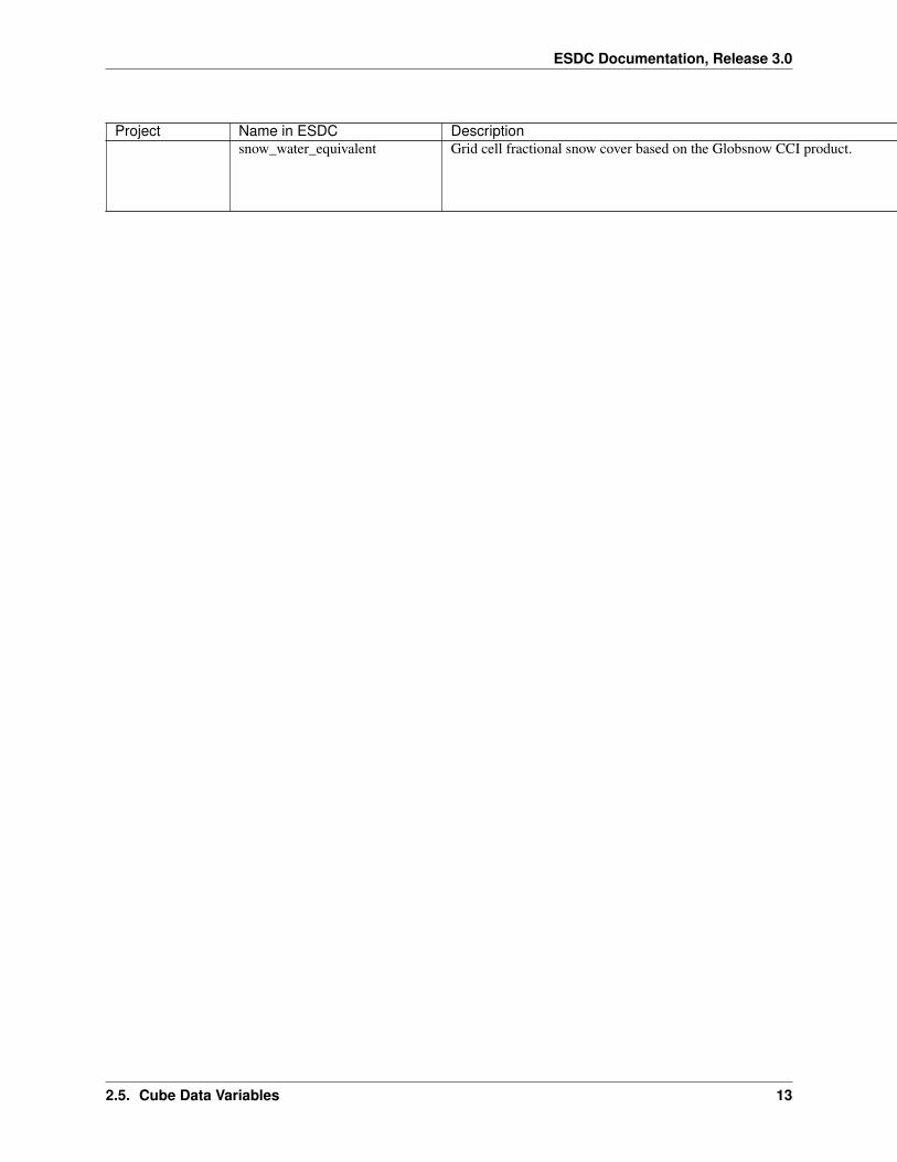
2.5 Cube Data Variables

Project Name in ESDC Description URL ReferencesGLEAM evaporative_stress Evaporative Stress Factor http://www.gleam.

euMartens, B.,Miralles, D.G.,Lievens, H., van derSchalie, R., de Jeu,R.A.M., Fernández-Prieto, D., Beck,H.E., Dorigo,W.A., and Verhoest,N.E.C.: GLEAMv3: satellite-basedland evaporationand root-zone soilmoisture, Geo-scientific ModelDevelopment, 10,1903–1925, 2017.

evaporation Evaporation

snow_sublimation Snow Sublimation

potential_evaporation Potential Evaporation

interception_loss Interception Loss

bare_soil_evaporation Bare Soil Evaporation

open_water_evaporation Open-water Evaporationsurface_moisture Surface Soil Moisturetranspiration Transpirationroot_moisture Root-Zone Soil Moisture

GFED4 burnt_area Burnt Area based on the GFED4 fire product. http://www.globalfiredata.org/

Giglio, Louis,James T. Rander-son, and Guido R.Werf. “Analysis ofdaily, monthly, andannual burned areausing the fourthgen-eration global fireemissions database(GFED4).” Journalof GeophysicalResearch: Bio-geosciences 118.1(2013): 317-328.

Continued on next page

2.5. Cube Data Variables 11

ESDC Documentation, Release 3.0

Table 1 – continued from previous pageProject Name in ESDC Description URL References

c_emissions Carbon emissions by fires based on the GFED4 fire product.

ESA Aerosol CCI aerosol_optical_thickness_865 Aerosol optical thickness derived from the dataset produced by the Aerosol CCI project. http://www.esa-aerosol-cci.org/

Holzer-Popp, T.,de Leeuw, G.,Griesfeller, J.,Martynenko, D.,Klueser, L., Bevan,S., et al. (2013).Aerosol retrievalexperiments in theESA Aerosol_cciproject. Atmo-spheric Measure-ment Techniques,6, 1919-1957.doi:10.5194/amt-6-1919-2013.

aerosol_optical_thickness_1610 Aerosol optical thickness derived from the dataset produced by the Aerosol CCI project.

aerosol_optical_thickness_550 Aerosol optical thickness derived from the dataset produced by the Aerosol CCI project.

aerosol_optical_thickness_659 Aerosol optical thickness derived from the dataset produced by the Aerosol CCI project.

aerosol_optical_thickness_555 Aerosol optical thickness derived from the dataset produced by the Aerosol CCI project.

GlobTemperature land_surface_temperature Advanced Along Track Scanning Radiometer pixel land surface temperature product http://data.globtemperature.info/ Jiménez, C., et al. “Inversion of AMSRE observations for land surface temperature estimation: 1. Methodology and evaluation with station temperature.” Journal of Geophysical Research: Atmospheres 122.6 (2017): 3330-3347.ERAInterim air_temperature_2m Air temperature at 2m from the ERAInterim reanalysis product. http://www.ecmwf.int/en/research/climate-reanalysis/era-interim Dee, D.P. et al. 2011 http://onlinelibrary.wiley.com/doi/10.1002/qj.828/abstractSoilMoisture CCI soil_moisture Soil moisture based on the SOilmoisture CCI project http://www.esa-soilmoisture-cci.org Liu, Y.Y., Parinussa, R.M., Dorigo, W.A., De Jeu, R.A.M., Wagner, W., McCabe, M.F., Evans, J.P., and van Dijk, A.I.J.M. (2012): Trend-preserving blending of passive and active microwave soil moisture retrievals; Liu, Y.Y., Parinussa, R.M., Dorigo, W.A., De Jeu, R.A.M., Wagner, W., van Dijk, A.I.J.M., McCabe, M.F., & Evans, J.P. (2011): Developing an improved soil moisture dataset by blending passive and active microwave satellite based retrievals. Hydrology and Earth System Sciences, 15, 425-436.GlobVapour water_vapour Total column water vapour based on the GlobVapour CCI product. http://www.globvapour.info/ Schneider, Nadine, et al. “ESA DUE GlobVapour water vapor products: Validation.” AIP Conference Proceedings. Vol. 1531. No. 1. 2013.Ozone CCI ozone Atmospheric ozone based on the Ozone CCI data. http://www.esa-ozone-cci.org/ Laeng, A., et al. “The ozone climate change initiative: Comparison of four Level-2 processors for the Michelson Interferometer for Passive Atmospheric Sounding (MIPAS).” Remote Sensing of Environment 162 (2015): 316-343.GlobAlbedo white_sky_albedo White sky albedo derived from the GlobAlbedo CCI project dataset http://www.

globalbedo.org/Muller, Jan-Peter,et al. “The ESAGLOBALBEDOproject for mappingthe Earth’s landsurface albedofor 15 years fromEuropean sensors.”Geophysical Re-search Abstracts.Vol. 13. 2012.

black_sky_albedo Black sky albedo derived from the GlobAlbedo CCI project dataset

FLUXCOM net_ecosystem_exchange Net carbon exchange between the ecosystem and the atmopshere. http://www.fluxcom.org/

Tramontana, Gi-anluca, et al.“Predicting carbondioxide and energyfluxes across globalFLUXNET siteswith regressionalgorithms.” (2016).

terrestrial_ecosystem_respiration Total carbon release of the ecosystem through respiration.

gross_primary_productivity Gross Carbon uptake of of the ecosystem through photosynthesis

latent_energy Latent heat flux from the surface.sensible_heat Sensible heat flux from the surface

GPCP precipitation Precipitation based on the GPCP dataset. http://precip.gsfc.nasa.gov/ Adler, Robert F., et al. “The version-2 global precipitation climatology project (GPCP) monthly precipitation analysis (1979-present).” Journal of hydrometeorology 4.6 (2003): 1147-1167.GlobSnow fractional_snow_cover Grid cell fractional snow cover based on the Globsnow CCI product. http://www.

globsnow.info/Luojus, Kari, etal. “ESA DUEGlobsnow-GlobalSnow Database forClimate Research.”ESA Special Pub-lication. Vol. 686.2010.

Continued on next page

12 Chapter 2. ESDC Description

ESDC Documentation, Release 3.0

Table 1 – continued from previous pageProject Name in ESDC Description URL References

snow_water_equivalent Grid cell fractional snow cover based on the Globsnow CCI product.

2.5. Cube Data Variables 13

ESDC Documentation, Release 3.0

14 Chapter 2. ESDC Description

CHAPTER 3

ESDC Access

As introduced in the last section, the ESDC physically consists of a set of NetCDF files on disk, which can be accessedin a number of different ways which are described in this section.

3.1 Download ESDC Data

The simplest approach to access the ESDC data is downloading it to you computer using the ESDC FTP server.

Since the ESDC is basically a directory of NetCDF files, you can use a variety of software packages and programminglanguages to access the data. In each cube directory, you find a text file cube.config which describes the overalldata cube layout.

Within the ESDC Project, dedicated data access packages have been developed for the Python and Julia programminglanguages. These packages “understand” the ESDC’s cube.config files and represent the cube data by a convenientdata structures. The section Using Python describes how to access the data from Python.

3.2 OPeNDAP and WCS Services

The ESDC’ data variables can also be accessed via a dedicated ESDC THREDDS server.

The server supports the OPeNDAP and OGC-compliant Web Coverage Service (WCS) data access protocols. You canuse it for accessing subsets of the ESDC’s data variables and also for visual exploration of the data, and finally fordownloading the data as a NetCDF file or of plain text.

Depending on the variable subsets, and the region and time period of interest, the transferred data volume might bemuch lower than a complete download of the ESDC via FTP. However, the disadvantage of using OPeNDAP and WCSis that the actual structure of the ESDC gets lost, so that it can’t be accessed anymore using the aforementioned ESDCPython/Julia data access packages.

15

ESDC Documentation, Release 3.0

3.3 E-Laboratory

A dedicated ESDC E-Laboratory has been developed to access the ESDC data via distributed Jupyter Notebooks forJulia and Python. This is the most resource efficient and convenient way of exploring the ESDC.

These notebooks have direct access to the ESDC data so there is no need to download it. In addition they provide theESDC Python and Julia APIs comprising the Data Access API and the Data Analytics Toolkit.

The E-Laboratory provides some example notebooks in the shared ESDC community repository.

The E-Laboratory is based on the JupyterHub platform and currently comprises three 16-core computers running in aCloud environment.

3.4 Using Python

3.4.1 Installation

Note: if you use the E-Laboratory you don’t need to install any additional packages for accessing the data. This sectionis only relevant if you’ve downloaded a ESDC instance to your local computer.

While in principle the NetCDF files comprising the ESDC can be used with any tool of choice, we developed specifi-cally tailored Data Access APIs for Python 3.X and Julia. Furthermore, a set of high-level routines for data analysis,the Data Analytics Toolkit, greatly facilitates standard operations on the large amount of data in the ESDC. While inthe E-laboratory, the Data Access API and the DAT are already pre-installed, the user has to download and install thecube library when working on a local computer.

The ESDC Python package has been developed against latest Anaconda / Miniconda distributions and uses their Condapackage manager.

To get started on your local computer with Python, clone the cablab-core repository from https://github.com/CAB-LAB:

git clone https://github.com/CAB-LAB/cablab-core

The following command will create a new Python 3.5 environment named esdc with all required dependencies,namely

• dask >= 0.14

• gridtools >= 0.1 (from Conda channel forman)

• h5netcdf >= 0.3

• h5py >= 2.7

• netcdf4 >= 1.2

• scipy >= 0.16

• scikit_image >= 0.11

• matplotlib >= 2.0

• xarray >= 0.9

$ conda env create environment.yml

To active new Python environment named esdc you must source on Linux/Darwin

16 Chapter 3. ESDC Access

ESDC Documentation, Release 3.0

$ source activate.sh esdc

on Windows:

> activate esdc

Now change into new folder cablab-core and install the cablab Python package using the develop target:

$ cd cablab-core$ python setup.py develop

You can now easily change source code in cablab-core without reinstalling it. When you do not plan to add ormodify any code (e.g. add a new source data provider), you can also permanently install the sources using

$ python setup.py install

However, if you now change any code, make sure to the install command again.

After download of a ESDC including the corresponding cube.config file and successful installation of the ESDC,you are ready to explore the data in the ESDC using the Using Python.

3.4.2 Usage

The following example code demonstrates how to access a locally stored ESDC, query its content, and get data chunksof different sizes for further analysis.

Open a cube

from cablab import Cubefrom datetime import datetimeimport numpy as np

cube = Cube.open("/path/to/datacube")

Note, in order to work properly the /path/to/datacube/ passed to Cube.open() must be the path to anexisting ESDC cube directory which contains a valid configuration file named cube.config. It contains essentialmetadata about the ESDC to be opened.

cube.data.variable_names

['aerosol_optical_thickness_1610','aerosol_optical_thickness_550','aerosol_optical_thickness_555','aerosol_optical_thickness_659','aerosol_optical_thickness_865','air_temperature_2m','bare_soil_evaporation','black_sky_albedo','burnt_area','country_mask','c_emissions',...]

After successful opening the ESDC, chunks of data or the entire data set can be accessed via the dataset()and get() functions. The first returns a xarray.Dataset object in which all cube variables are represented as xar-ray.DataArray objects. More about these objects can also be found in DAT for Python section. The second function

3.4. Using Python 17

ESDC Documentation, Release 3.0

can be used to read subsets of the data. In contrast it returns a list of Numpy ndarray arrays, one for each requestedvariable.

The corresponding API for Julia is very similar and illustrated in DAT for Julia.

Accessing the cube data

The cube.data.dataset() has an optional argument which is a list of variable names to include in the returnedxarray.DataArray object. If omitted, all variables will be included. Note it can take up to a few seconds to opengenerate the dataset object with all variables.

ds = cube.data.dataset()ds

<xarray.Dataset>Dimensions: (bnds: 2, lat: 720, lon: 1440, time:

→˓506)Coordinates:

* time (time) datetime64[ns] 2001-01-05 ...

* lon (lon) float32 -179.875 -179.625 ...lon_bnds (lon, bnds) float32 -180.0 -179.75 ...lat_bnds (lat, bnds) float32 89.75 90.0 89.5 ...

* lat (lat) float32 89.875 89.625 89.375 ...time_bnds (time, bnds) datetime64[ns] 2001-01-01

→˓...Dimensions without coordinates: bndsData variables:

aerosol_optical_thickness_1610 (time, lat, lon) float64 nan nan nan ..→˓.

aerosol_optical_thickness_550 (time, lat, lon) float64 nan nan nan ..→˓.

aerosol_optical_thickness_555 (time, lat, lon) float64 nan nan nan ..→˓.

aerosol_optical_thickness_659 (time, lat, lon) float64 nan nan nan ..→˓.

aerosol_optical_thickness_865 (time, lat, lon) float64 nan nan nan ..→˓.

air_temperature_2m (time, lat, lon) float64 243.4 243.4 ..→˓.

bare_soil_evaporation (time, lat, lon) float64 nan nan nan ..→˓.

black_sky_albedo (time, lat, lon) float64 nan nan nan ..→˓.

burnt_area (time, lat, lon) float64 0.0 0.0 0.0 ..→˓.

country_mask (time, lat, lon) float64 nan nan nan ..→˓.

...

lst = ds['land_surface_temperature']lst

<xarray.DataArray 'land_surface_temperature' (time: 506, lat: 720, lon: 1440)>dask.array<concatenate, shape=(506, 720, 1440), dtype=float64, chunksize=(46,

→˓720, 1440)>Coordinates:

18 Chapter 3. ESDC Access

ESDC Documentation, Release 3.0

* time (time) datetime64[ns] 2001-01-05 2001-01-13 2001-01-21 ...

* lon (lon) float32 -179.875 -179.625 -179.375 -179.125 -178.875 ...

* lat (lat) float32 89.875 89.625 89.375 89.125 88.875 88.625 88.375 ..→˓.Attributes:

url: http://data.globtemperature.info/long_name: land surface temperaturesource_name: LSTstandard_name: surface_temperaturecomment: Advanced Along Track Scanning Radiometer pixel land surfa.

→˓..units: K

The variable lst can now be used like a Numpy ndarray. Howver, using xarray there are a number of moreconvenient data access methods that take care of the actual coordinates provided for every dimenstion. For example,the sel() method can be used to extract slices and subsets from a data array. Here a point is extract from lst, andthe result is a 1-element data array:

lst_point = lst.sel(time='2006-06-15', lat=53, lon=11, method='nearest')lst_point

<xarray.DataArray 'land_surface_temperature' ()>dask.array<getitem, shape=(), dtype=float64, chunksize=()>Coordinates:

time datetime64[ns] 2006-06-14lon float32 11.125lat float32 53.125

Attributes:url: http://data.globtemperature.info/long_name: land surface temperaturesource_name: LSTstandard_name: surface_temperaturecomment: Advanced Along Track Scanning Radiometer pixel land surfa...units: K

Data arrays also have a handy plot() method. Try:

lst.sel(lat=53, lon=11, method='nearest').plot()lst.sel(time='2006-06-15', method='nearest').plot()lst.sel(lon=11, method='nearest').plot()lst.sel(lat=53, method='nearest').plot()

Closing the cube

If you no longer require access to the cube, it should be closed to release file handles and reserved memory.

cube.close()

Some more demonstrations are included in the ESDC community notebooks.

3.5 Using Julia

The Data Access API for Julia is part of the DAT for Julia.

3.5. Using Julia 19

ESDC Documentation, Release 3.0

3.6 Data Analysis

In addition to the Data Access APIs, we provide a Data Analytics Toolkit (DAT) to facilitate analysis and visualizationof the ESDC. Please see

• DAT for Julia

• DAT for Python

20 Chapter 3. ESDC Access

CHAPTER 4

ESDC Generation

This section explains how a ESDC is generated and how it can be extended by new variables.

4.1 Command-Line Tool

To generate new data cubes or to update existing ones a dedicated command-line tool cube-gen is used.

After installing cablab-core as described in section Installation, try:

$ cube-gen --help

CAB-LAB command-line interface, version 0.2.2usage: cube-gen [-h] [-l] [-G] [-c CONFIG] [TARGET] [SOURCE [SOURCE ...]]

Generates a new CAB-LAB data cube or updates an existing one.

positional arguments:TARGET data cube root directorySOURCE <provider name>:dir=<directory>, use -l to list source

provider names

optional arguments:-h, --help show this help message and exit-l, --list list all available source providers-G, --dont-clear-cache

do not clear data cache before updating the cube(faster)

-c CONFIG, --cube-conf CONFIGdata cube configuration file

The list option lists all currently installed source data providers:

21

ESDC Documentation, Release 3.0

$ cube-gen --list

ozone -> cablab.providers.ozone.OzoneProvidernet_ecosystem_exchange -> cablab.providers.mpi_bgc.MPIBGCProviderair_temperature -> cablab.providers.air_temperature.AirTemperatureProviderinterception_loss -> cablab.providers.gleam.GleamProvidertranspiration -> cablab.providers.gleam.GleamProvideropen_water_evaporation -> cablab.providers.gleam.GleamProvider...

Source data providers are the pluggable software components used by cube-gen to read data from a source directoryand transform it into a common data cube structure. The list above shows the mapping from short names to be usedby the cube-gen command-line to the actual Python code, e.g. for ozone, the OzoneProvider class of thecablab/providers/ozone.py module is used.

The common cube structure is established by a cube configuration file provided by the cube-config option. Hereis the configuration file that is used to produce the low-resolution ESDC. It will produce a 0.25 degrees global cubethat whose source data will aggregated/interpolated to match 8 day periods and then resampled to match 1440 x 720spatial grid cells:

model_version = '0.2.4'spatial_res = 0.25temporal_res = 8grid_width = 1440grid_height = 720start_time = datetime.datetime(2001, 1, 1, 0, 0)end_time = datetime.datetime(2012, 1, 1, 0, 0)ref_time = datetime.datetime(2001, 1, 1, 0, 0)calendar = 'gregorian'file_format = 'NETCDF4_CLASSIC'compression = False

To create or update a cube call the cube-gen tool with the configuration and the cube data provider(s). The cubedata providers can have parameters on their own. All current providers have the dir parameter indicating the sourcedata directory but this is not a rule. Other providers which read from multivariate sources also have a var parameterto indicate which variable of many possible should be used.

$ cube-gen mycube -c mycube.config ozone:dir=/path/to/ozone/netcdfs

will create the cube mycube in current directory using the mycube.config configuration and add a single variableozone from source NetCDF files in /path/to/ozone/netcdfs.

Note, the GitHub repository cube-config is used to keep the configurations of individual ESDC versions.

4.2 Writing a new Provider

In order to add new source data for which there is no source data provider yet, you can write your own.

Make sure cablab-core is installed as described in section Installation above.

If your source data is NetCDF, writing a new provider is easy. Just copy one of the existing providers, e.g. ca-blab/providers/ozone.py and start adopting the code to your needs.

For source data other than NetCDF, you will have to write a provider from scratch by implementing the cablab.CubeSourceProvider interface or by extending the cablab.BaseCubeSourceProvider which is usuallyeasier. Make sure you adhere to the contract described in the documentation of the respective class.

22 Chapter 4. ESDC Generation

ESDC Documentation, Release 3.0

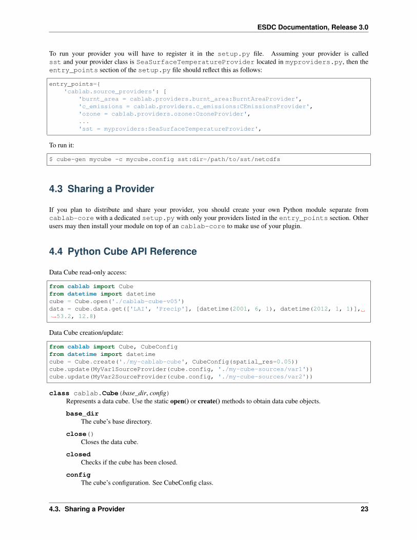
To run your provider you will have to register it in the setup.py file. Assuming your provider is calledsst and your provider class is SeaSurfaceTemperatureProvider located in myproviders.py, then theentry_points section of the setup.py file should reflect this as follows:

entry_points={'cablab.source_providers': [

'burnt_area = cablab.providers.burnt_area:BurntAreaProvider','c_emissions = cablab.providers.c_emissions:CEmissionsProvider','ozone = cablab.providers.ozone:OzoneProvider',...'sst = myproviders:SeaSurfaceTemperatureProvider',

To run it:

$ cube-gen mycube -c mycube.config sst:dir=/path/to/sst/netcdfs

4.3 Sharing a Provider

If you plan to distribute and share your provider, you should create your own Python module separate fromcablab-core with a dedicated setup.py with only your providers listed in the entry_points section. Otherusers may then install your module on top of an cablab-core to make use of your plugin.

4.4 Python Cube API Reference

Data Cube read-only access:

from cablab import Cubefrom datetime import datetimecube = Cube.open('./cablab-cube-v05')data = cube.data.get(['LAI', 'Precip'], [datetime(2001, 6, 1), datetime(2012, 1, 1)],→˓53.2, 12.8)

Data Cube creation/update:

from cablab import Cube, CubeConfigfrom datetime import datetimecube = Cube.create('./my-cablab-cube', CubeConfig(spatial_res=0.05))cube.update(MyVar1SourceProvider(cube.config, './my-cube-sources/var1'))cube.update(MyVar2SourceProvider(cube.config, './my-cube-sources/var2'))

class cablab.Cube(base_dir, config)Represents a data cube. Use the static open() or create() methods to obtain data cube objects.

base_dirThe cube’s base directory.

close()Closes the data cube.

closedChecks if the cube has been closed.

configThe cube’s configuration. See CubeConfig class.

4.3. Sharing a Provider 23

ESDC Documentation, Release 3.0

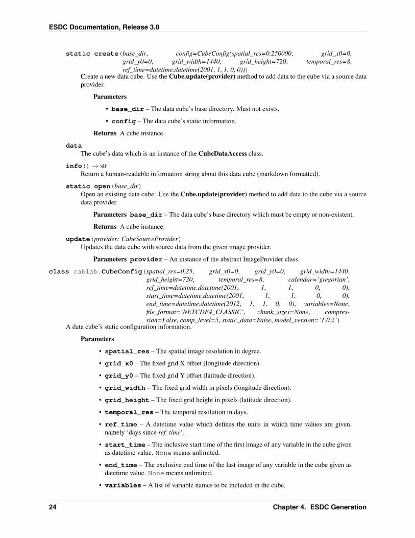
static create(base_dir, config=CubeConfig(spatial_res=0.250000, grid_x0=0,grid_y0=0, grid_width=1440, grid_height=720, temporal_res=8,ref_time=datetime.datetime(2001, 1, 1, 0, 0)))

Create a new data cube. Use the Cube.update(provider) method to add data to the cube via a source dataprovider.

Parameters

• base_dir – The data cube’s base directory. Must not exists.

• config – The data cube’s static information.

Returns A cube instance.

dataThe cube’s data which is an instance of the CubeDataAccess class.

info()→ strReturn a human-readable information string about this data cube (markdown formatted).

static open(base_dir)Open an existing data cube. Use the Cube.update(provider) method to add data to the cube via a sourcedata provider.

Parameters base_dir – The data cube’s base directory which must be empty or non-existent.

Returns A cube instance.

update(provider: CubeSourceProvider)Updates the data cube with source data from the given image provider.

Parameters provider – An instance of the abstract ImageProvider class

class cablab.CubeConfig(spatial_res=0.25, grid_x0=0, grid_y0=0, grid_width=1440,grid_height=720, temporal_res=8, calendar=’gregorian’,ref_time=datetime.datetime(2001, 1, 1, 0, 0),start_time=datetime.datetime(2001, 1, 1, 0, 0),end_time=datetime.datetime(2012, 1, 1, 0, 0), variables=None,file_format=’NETCDF4_CLASSIC’, chunk_sizes=None, compres-sion=False, comp_level=5, static_data=False, model_version=’1.0.2’)

A data cube’s static configuration information.

Parameters

• spatial_res – The spatial image resolution in degree.

• grid_x0 – The fixed grid X offset (longitude direction).

• grid_y0 – The fixed grid Y offset (latitude direction).

• grid_width – The fixed grid width in pixels (longitude direction).

• grid_height – The fixed grid height in pixels (latitude direction).

• temporal_res – The temporal resolution in days.

• ref_time – A datetime value which defines the units in which time values are given,namely ‘days since ref_time’.

• start_time – The inclusive start time of the first image of any variable in the cube givenas datetime value. None means unlimited.

• end_time – The exclusive end time of the last image of any variable in the cube given asdatetime value. None means unlimited.

• variables – A list of variable names to be included in the cube.

24 Chapter 4. ESDC Generation

ESDC Documentation, Release 3.0

• file_format – The file format used. Must be one of ‘NETCDF4’,‘NETCDF4_CLASSIC’, ‘NETCDF3_CLASSIC’ or ‘NETCDF3_64BIT’.

• chunk_sizes – A mapping of dimension names to chunk size for encoding. Default isNone.

• compression – Whether gzip compression is used for encoding. Default is False.

• comp_level – Integer between 1 and 9 describing the level of compression desired forencoding. Default is 5. Ignored if compression is False.

date2num(date)→ floatReturn the number of days for the given date as a number in the time units given by the time_unitsproperty.

Parameters date – The date as a datetime.datetime value

eastingThe latitude position of the upper-left-most corner of the upper-left-most grid cell given by (grid_x0,grid_y0).

geo_boundsThe geographical boundary given as ((LL-lon, LL-lat), (UR-lon, UR-lat)).

static load(path)→ objectLoad a CubeConfig from a text file.

Parameters path – The file’s path name.

Returns A new CubeConfig instance

northingThe longitude position of the upper-left-most corner of the upper-left-most grid cell given by (grid_x0,grid_y0).

num_periods_per_yearReturn the integer number of target periods per year.

store(path)Store a CubeConfig in a text file.

Parameters path – The file’s path name.

time_unitsReturn the time units used by the data cube as string using the format ‘days since ref_time’.

4.4. Python Cube API Reference 25

ESDC Documentation, Release 3.0

26 Chapter 4. ESDC Generation

CHAPTER 5

DAT for Julia

5.1 Overview

The Data Analytics Toolkit (DAT) for Julia is hosted in CABLAB’s github repository and is developed in closeinteraction with the scientific community. Here we give a short overview on the capabilities of the Julia DAT, butwe would refer to the official documentation for a more detailed and frequently updated software description.

The current implementation of the Julia DAT consists of 3 parts:

1. A collection of analysis functions that can be applied to the ESDC

2. Functions for visualizing time-series and spatial maps

3. A function to register custom functions to be applied on the cube

1. Collection of analysis functions

We provide several methods to perform basic statistical analyses on the ESDC. In a typical workflow, the user wantsto apply some function (e.g. a time series analysis) on all points of the cube. In other systems this would mean thatthe user must write some loop that reads chunks of data, applies the function, stores the result and then read the nextchunk of data etc. In the Julia DAT, this is done automatically, the user just calls e.g. mapCube(removeMSC,mycube)and the mean seasonal cycle will be subtracted from all individual time series contained in the selected cube.

In Analysis one can find a list of all currently implemented DAT methods.

2. Visualisation of the ESDC

For a convenient and interactive visual inspection of the ESDC five plotting functions are available:

• plotXY for scatterplotd or bar plots along a single axis

• plotTS like plotXY but the x axis set to TimeAxis by default

• plotScatter for scatter plots of two elements from the same axis, e.g. of two Variables

• plotMAP for generic map plots

• plotMAPRGB for RGB-like maps plots where different variables can be mapped to the plot color channels

27

ESDC Documentation, Release 3.0

For examples and a detailed description of the plotting functions, see Plotting

3. Adding user functions into the DAT

Users can add custom functions to the DAT for individual sessions. This is described in detail in the adding_newchapter of the manual.

5.2 Use Cases and Examples

Example notebooks that explore the ESDC using the Julia DAT can be found in the cablab-shared repository.

28 Chapter 5. DAT for Julia

CHAPTER 6

DAT for Python

6.1 Overview

The main objective of the Data Analytics Toolkit is to facilitate the exploitation of the multi-variate data set in theESDC for experienced users and empower less experienced users to explore the wealth of information contained inthe ESDC. To this end, Python is almost a natural choice for the programming language, as it is easy to learn and use,offers numerous, well-maintained community packages for data handling and analysis, statistics, and visualisation.

The DAT for Python relies primarily on xarray a package that provides N-dimensional data structures and efficientcomputing methods on those object. In fact, xarray closely follows the approach adopted NetCDF, the quasi-standardfile format for geophysical data, and provides methods for many commonly executed operations on spatial data. Thecentral data structure used for representing the ESDC in Python is thus the xarray.Dataset.

Such dataset objects are what you get when accessing the cube’s data as follows:

from cablab import Cubecube = Cube.open("/home/doe/esdc/cablab-datacube-0.2.4/low-res")dataset = cube.data.dataset(["precipitation", "evaporation", "ozone", "soil_moisture",→˓"air_temperature_2m"])

Any geo-physical variable in the ESDC is represented by a xarray.DataArray, which are Numpy-like data arrays withadditional coordinate information and metadata.

The following links point into the xarray documentation, they provide the low-level interface for the Python DAT:

• Indexing and selecting data

• Computation

• Split-apply-combine

• Reshaping and reorganizing data

• Combining data

• Time series data

29

ESDC Documentation, Release 3.0

Building on top of the xarray API the DAT offers high-level functions for ESDC-specific workflows in the cablab.datmodule. These functions are addressing specific user requirements and the scope of the module will increase with theusers of the DAT. In the following, typical use cases and examples provide an illustrative introduction into the usageof the DAT and thus into the exploration of the ESDC.

6.2 Use Cases and Examples

The below examples are all contained in a Jupyter notebook, which is also available in the E-Lab.

6.2.1 Data Access and Indexing

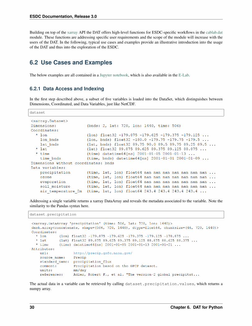
In the first step described above, a subset of five variables is loaded into the DataSet, which distinguishes betweenDimensions, Coordinated, and Data Variables, just like NetCDF.

dataset

Addressing a single variable returns a xarray DataArray and reveals the metadata associated to the variable. Note thesimilarity to the Pandas syntax here.

dataset.precipitation

The actual data in a variable can be retrieved by calling dataset.precipitation.values, which returns anumpy array.

30 Chapter 6. DAT for Python

ESDC Documentation, Release 3.0

isinstance (dataset.precipitation.values,np.ndarray)

xarray offers different ways for indexing, both integer and label-based look-ups, and the reader is referred to theexhaustive section in the respective section of the xarray documentation: xarray Indexing and selecting data. Thefollowing example, in which a chunk is cut out from the larger data set, demonstrates the convenience of xarrayssyntax. The result is again a xarray DataArray, but with only subset of variables and restricted to a smaller domain inlatitude and longitude.

dataset[['precipitation', 'evaporation']].sel(lat = slice(70.,30.), lon = slice(-20.,→˓35.))

6.2.2 Computation

It was a major objective of the Python DAT to facilitate processing and analysis of big, multivariate geophysical datasets like the ESDC. Typical use cases include the execution of functions on all data in the ESDC, the aggregationof data along a common axis, or analysing the relation between different variables in the data set. The followingexamples shed a light on the capabilities of the DAT, more typical examples can be found in the Jupyter notebook andthe documentation of xarray provides an exhaustive reference to the package’s functionalities.

Many generic mathematical functions are implemented for DataSets and DataArrays. For example, an average overall variables in the dataset can thus be easily calculated.

dataset.mean(skipna=True)

Note that calculating a simple average on a big data set may require more resources, particularly memory, than isavailable on the machine you are working at. In such cases, xarray automatically involves a package called dask forout-of-core computations and automatic parallelisation. Make sure that dask is installed to significantly improve theuser experience with the DAT. Similar to pandas, several computation methods like groupby or apply have beenimplemented for DataSets and DataArrays. In combination with the datetime data types, a monthly mean of a variablecan be calculated as follows:

6.2. Use Cases and Examples 31

ESDC Documentation, Release 3.0

dataset.air_temperature_2m.groupby('time.month').mean(dim='time')

In the resulting DataArray, a new dimension month has been automatically introduced. Users may also define theirown functions and apply them to the data. In the below example, zcores are computed for the entire DataSet by usigthe built-in functions mean and std. The user function above_Nsigma is applied to all data to test if a zscore isabove or below two sigma, i.e. is an outlier. The result is again a DataSet with boolean variables.

def above_Nsigma(x,Nsigma):return xr.ufuncs.fabs(x)>Nsigma

zscores = (dataset-dataset.mean(dim='time'))/dataset.std(dim='time')res = zscores.apply(above_Nsigma,Nsigma = 2)res

In addition to the functions and methods xarray is providing, we have begun to develop high-level functions thatsimplify typical operations on the ESDC. The function corrcf computes the correlation coefficient between twovariables.

6.2.3 Plotting

Plotting is key for the explorative analysis of data and for the presentation of results. This is of course even more sofor Earth System Data. Python offers many powerful approaches to meet the diverse visualisation needs of differentuse cases. Most of them can be used with the ESDC since the data can be easily transferred to numpy arrays or pandasdata frames. The following examples may provide a good starting point for developing more specific plots.

Calculating the correlation coefficient of two variables and plot the resulting 2D image af latitude and longitude.

cv = DAT_corr(dataset, 'precipitation', 'evaporation')cv.plot.imshow(vmin = -1., vmax = 1.)

32 Chapter 6. DAT for Python

ESDC Documentation, Release 3.0

Plotting monthly air temperature in twelve subplots.

Air_temp_monthly = dataset.air_temperature_2m.groupby('time.month').mean(dim='time')Air_temp_monthly.plot.imshow(x='lon',y='lat',col='month',col_wrap=3)

A simple time-series plot at a given location.

dataset.evaporation.sel(lon = 12.67,lat = 41.83, method = 'nearest').plot()

6.2. Use Cases and Examples 33

ESDC Documentation, Release 3.0

Plotting a projected map using the DAT function map_plot. .. code-block:: python

fig, ax, m = map_plot(dataset,’evaporation’,‘2006-03-01’,vmax = 6.)

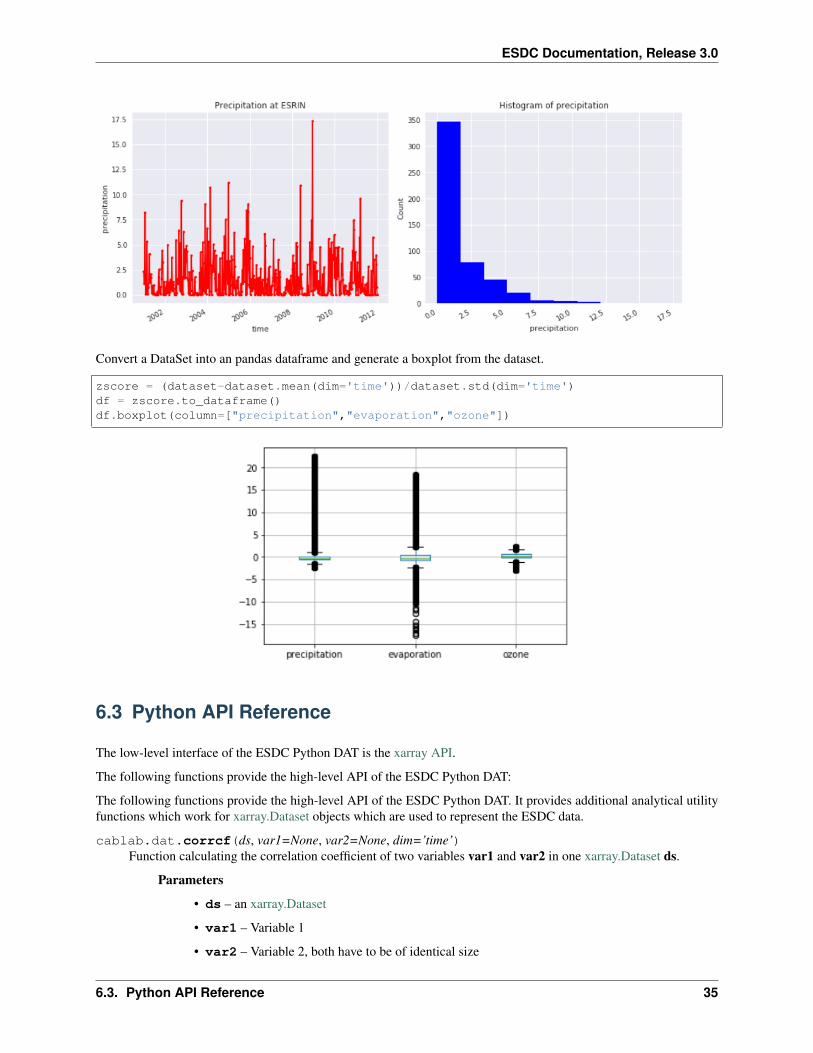
Generating a subplot of a time-series at a given location and the associated histogram of the data.

precip1d = dataset['precipitation'].sel(lon = 12.67,lat = 41.83, method = 'nearest')fig, ax = plt.subplots(figsize = [12,5], ncols=2)precip1d.plot(ax = ax[0], color ='red', marker ='.')ax[0].set_title("Precipitation at ESRIN")precip1d.plot.hist(ax = ax[1], color ='blue')ax[1].set_xlabel("precipitation")plt.tight_layout()

34 Chapter 6. DAT for Python

ESDC Documentation, Release 3.0

Convert a DataSet into an pandas dataframe and generate a boxplot from the dataset.

zscore = (dataset-dataset.mean(dim='time'))/dataset.std(dim='time')df = zscore.to_dataframe()df.boxplot(column=["precipitation","evaporation","ozone"])

6.3 Python API Reference

The low-level interface of the ESDC Python DAT is the xarray API.

The following functions provide the high-level API of the ESDC Python DAT:

The following functions provide the high-level API of the ESDC Python DAT. It provides additional analytical utilityfunctions which work for xarray.Dataset objects which are used to represent the ESDC data.

cablab.dat.corrcf(ds, var1=None, var2=None, dim=’time’)Function calculating the correlation coefficient of two variables var1 and var2 in one xarray.Dataset ds.

Parameters

• ds – an xarray.Dataset

• var1 – Variable 1

• var2 – Variable 2, both have to be of identical size

6.3. Python API Reference 35

ESDC Documentation, Release 3.0

• dim – dimension for aggregation, default is time. In the default case, the result is an image

Returns

cablab.dat.map_plot(ds, var=None, time=0, title_str=’No title’, projection=’kav7’, lon_0=0, resolu-tion=None, **kwargs)

Function plotting a projected map for a variable var in xarray.Dataset ds.

Parameters

• ds – an xarray.Dataset

• var – variable to plot

• time – time step or datetime date to plot

• title_str – Title string

• projection – for Basemap

• lon_0 – longitude 0 for central

• resolution – resolution for Basemap object

• kwargs – Any other kwargs accepted by the pcolormap function of Basemap

Returns

36 Chapter 6. DAT for Python

CHAPTER 7

Collaboration

Collaboration is at the heart of science!

The CAB-LAB project explicitly aims at enabling more scientists from various disciplines to not only interact withEarth System data, but also with each other. The CAB-LAB team seeks active exchange with users of any background,data owners willing to add their data to the ESDC, and developers who are interested in improving the ESDC.

There are several ways to get in contact with the CAB-LAB team and other users of the ESDC:

7.1 Code Repository

The source code is currently and will be for the foreseeable future under continuous development. Since the CAB-LABteam takes collaboration, transparency, and reproducibility seriously, the project is open source and public from thevery beginning. Visit CAB-LAB’s github repository and check out the current status of the project or even contribute!

7.2 Website & Forum

Important updates on the project’s progress are frequently published on the CAB-LAB webpage: http://earthsystemdatacube.net. Moreover, in the forum of the webpage you can easily interact with project members andusers! Or simply write an email to info@earthsystemdatacube.net to get in contact with the project members.

37

ESDC Documentation, Release 3.0

38 Chapter 7. Collaboration

CHAPTER 8

Indices and Tables

• genindex

• search

39

ESDC Documentation, Release 3.0

40 Chapter 8. Indices and Tables

Index

Bbase_dir (cablab.Cube attribute), 23

Ccablab (module), 23cablab.dat (module), 35close() (cablab.Cube method), 23closed (cablab.Cube attribute), 23config (cablab.Cube attribute), 23corrcf() (in module cablab.dat), 35create() (cablab.Cube static method), 23Cube (class in cablab), 23Cube Spatial and Temporal Coverage, 7CubeConfig (class in cablab), 24

Ddata (cablab.Cube attribute), 24Data Policy, 5date2num() (cablab.CubeConfig method), 25

EEarth System Data Cube, 6easting (cablab.CubeConfig attribute), 25ESDC Macro Structure, 7

Ggeo_bounds (cablab.CubeConfig attribute), 25

Iinfo() (cablab.Cube method), 24

LLegal information, 5load() (cablab.CubeConfig static method), 25

Mmap_plot() (in module cablab.dat), 36

Nnorthing (cablab.CubeConfig attribute), 25num_periods_per_year (cablab.CubeConfig attribute), 25

Oopen() (cablab.Cube static method), 24

Sstore() (cablab.CubeConfig method), 25

Ttime_units (cablab.CubeConfig attribute), 25

Uupdate() (cablab.Cube method), 24

41