ESDU 80025 Endorsed by The Royal Aeronautical Society The Institution of Structural Engineers Mean forces, pressures and flow field velocities for circular cylindrical structures: single cylinder with two-dimensional flow Issued October 1980 With Amendments A to C June 1986 Supersedes ESDU 70013
Transcript
ESDU 80025
Endorsed byThe Royal Aeronautical SocietyThe Institution of Structural Engineers
Mean forces, pressures and flow fieldvelocities for circular cylindrical
structures:single cylinder with two-dimensional flow
Issued October 1980With Amendments A to C
June 1986Supersedes ESDU 70013
ESDU 80025ESDU DATA ITEMS
Data Items provide validated information in engineering design and analysis for use by, or under the supervisionof, professionally qualified engineers. The data are founded on an evaluation of all the relevant information, bothpublished and unpublished, and are invariably supported by original work of ESDU staff engineers or consultants.The whole process is subject to independent review for which crucial support is provided by industrial companies,government research laboratories, universities and others from around the world through the participation of someof their leading experts on ESDU Technical Committees. This process ensures that the results of much valuablework (theoretical, experimental and operational), which may not be widely available or in a readily usable form, canbe communicated concisely and accurately to the engineering community.
We are constantly striving to develop new work and review data already issued. Any comments arising out of youruse of our data, or any suggestions for new topics or information that might lead to improvements, will help us toprovide a better service.
THE PREPARATION OF THIS DATA ITEM
The work of on this particular Item was monitored and guided by the Wind Engineering Panel which has the followingconstitution:
The Panel has benefited from the participation of members from several engineering disciplines. In particular,Dr A.R. Flint has been appointed to represent the interests of structural engineering as the nominee of the Institutionof Structural Engineers.
(Continued on inside back cover)
ChairmanMr T.V. Lawson — Bristol University
MembersMr K.C. Anthony — Ove Arup and PartnersDr D.J. Cockrell — University of Leicester Prof. A.G. Davenport* — University of Western Ontario, CanadaDr A.R. Flint — Flint and NeillMr D.H. Freeston*
* Corresponding Member
— University of Auckland, New ZealandMr R.I. Harris — Cranfield Institute of TechnologyMr R.A. Lyons — Atkins Research and DevelopmentMr J.R. Mayne — Building Research EstablishmentMr R.J. Melling — Post Office TelecommunicationsDr G.A. Mowatt — CJB - Earl and Wright LtdMr J.R.C. Pedersen — IndependentMr D.J.W. Richards — Central Electricity Research LaboratoriesMr C. Scruton — IndependentMr R.E. Whitbread — National Maritime Institute.
ESDU 80025
MEAN FORCES, PRESSURES AND FLOW FIELD VELOCITIES FOR CIRCULAR CYLINDRICAL STRUCTURES: SINGLE CYLINDER WITH TWO-DIMENSIONAL FLOW
CONTENTS
Page
1. NOTATION AND UNITS 1
2. PURPOSE, SCOPE AND USE OF THIS DATA ITEM 32.1 Purpose 32.2 Scope 42.3 Use of the Data Item 42.4 Applicability, Limitations and Uncertainties 5
3. DRAG COEFFICIENT OF ISOLATED CYLINDER NORMAL TO FLOW 53.1 The Roughness Factor λR 63.2 The Turbulence Factor λT 73.3 Calculation Procedure For Evaluating CD0 73.4 Wind-tunnel Simulation of High Reynolds Number Flow 8
5. CYLINDERS WITH SURFACE IRREGULARITIES 115.1 Stranded Cables 115.2 Perforated Cylinders and Shrouds 11
5.2.1 Derivation 125.3 Effect of Fins and Strakes 125.4 Effect of Other Spanwise Protrusions 13
5.4.1 Comments on the effects of protrusions 14
6. PROXIMITY EFFECT OF PLANE SURFACE PARALLEL TO CYLINDER AXIS 15
7. MEAN AND FLUCTUATING PRESSURE DISTRIBUTIONS, VELOCITY FLOW FIELD 177.1 Mean Pressure Distribution at Surface 17
7.1.1 Derivation of method for mean pressure distribution at surface 187.2 Fluctuating Pressure Distribution at Surface 187.3 Velocity Flow Field Away From Surface 20
7.3.1 Derivation of velocity flow field parameters 20
i
ESDU 80025
8. EXAMPLES 208.1 Example 1 208.2 Example 2 218.3 Calculation Sheet for Examples (from Table 10.3) 238.4 Calculation Sheet for Example 1 (from Table 10.5) 24
9. REFERENCES AND DERIVATION 259.1 References 259.2 Derivation 25
10. TABLES 28
FIGURES 1 to 15 33 to 49
APPENDIX A GENERAL FEATURES OF THE FLOW AROUND A CIRCULAR CYLINDER 51
A1. CYLINDER WITH TWO-DIMENSIONAL FLOW 51
A2. INFLUENCE OF FREE-STREAM TURBULENCE 52
A3. INFLUENCE OF SURFACE ROUGHNESS 53
APPENDIX B SURFACE ROUGHNESS CHARACTERISTICS 55
B1. EQUIVALENT SAND GRAIN ROUGHNESS 55
B2. ADDITIONAL REFERENCES 56
B3. TABLE OF EQUIVALENT ROUGHNESS VALUES FOR VARIOUS TYPES OF SURFACE FINISH 56
APPENDIX C SUMMARY OF EQUATIONS FOR SOME OF THE GRAPHICAL DATA 57
C1. EQUATION FITS TO THE DATA 57
APPENDIX D RANGE OF EXPERIMENTAL DATA 60
D1. SOURCES AND RANGE OF DATA USED 60
ii
ESDU 80025
MEAN FORCES, PRESSURES AND FLOW FIELD VELOCITIES FOR CIRCULAR CYLINDRICAL STRUCTURES: Single Cylinder with Two-dimensional Flow
1. NOTATION AND UNITS
SI Unit
mean drag coefficient of two-dimensional circular cylinder whose longitudinal axis is normal to flow; drag force per unit
set of force coefficients acting along and normal to flow direction and to cylinder axes respectively (see Sketch 4.1); force per unit
mean pressure coefficient at cylinder surface,
instantaneous value of the fluctuating pressure coefficient
extreme value of Cp(t)
value of Cp on cylinder surface in wake region (see Sketch 7.1)
minimum value of Cp on cylinder surface (see Sketch 7.1)
mean pressure coefficient at distance r from cylinder centre and angle (see Sketch 7.2)
cylinder diameter m
protrusion height m
factor in Equation (4.7) accounting for effect of cylinder inclination on CN
crest or peak factor (see Equation (7.9))
gap width between cylinder and plane surface (see Sketch 6.1) m
intensities of turbulence; and (see Table 10.2 for typical values)
length of cylinder m
lateral integral scale of u-component of turbulence (see Table 10.2 for typical values)
m
local static pressure N/m3
Reynolds number,
CD0length/ ½ρV∞
2 D( )
CD ,CL
CN ,CT
length/ ½ρV∞2 D( )
Cp p p∞–( )/ ½ρV∞2( )
Cp t( )
Cp t( )
Cpb
Cpm
Cp r θ,( ) θ
D
d
fφ
g
h
Iu ,Iv σu/V∞ σv/V∞
L
Lr u
p
Re V∞D φ/νsec
Issued October 1980
1With Amendments A to C, June 1986 – 60 pages
ESDU 80025
critical Reynolds number, i.e. Re at which CD0 = 0.8 in rapid drag fall (see Appendix A)
effective Reynolds number, Re (see Section 3)
Re at which rapid fall in CD0 at transition begins (see Sketch 3.1)
distance between cylinder centre and point in flow field m
fluctuating components of free-stream velocity in direction of flow, and normal to flow direction and cylinder longitudinal axis, respectively
m/s
mean free-stream velocity m/s
local mean flow velocity at surface of cylinder m/s
local mean velocity in flow field at distance r from cylinder centre and angle
m/s
effective mean free-stream velocity in boundary layer (see Equation (6.1)) m/s
local mean free-stream velocity in boundary-layer flow (see Sketch 6.1) m/s
length of plane surface upstream of cylinder location m
power-law index giving approximate variation of Vz with height from surface
angle between local flow direction and free-stream direction (see Sketch 7.2) deg
effective roughness height of surface (see Table 10.1 for typical values) m
angular location of point (see Sketches 5.2, 7.1) deg
value of where Cp first equals Cpb deg
value of where Cp = Cpm deg
parameter defining effect of surface roughness on Ree (see Section 3.1)
parameter defining effect of flow turbulence on Ree (see Section 3.2)
kinematic viscosity of free-stream m2/s
density of free-stream kg/m3
standard deviation of fluctuating pressure coefficient
standard deviations of u(t) and v(t) m/s
Recrit
Ree λTλR
ReD
Rex V∞x/ν
r
u t( ) v t( ),
V∞
Vs
V r θ;( )θ
Veff
Vz
x
α
β r θ;( )
ε
θ
θb θ
θm θ
λR
λT
ν
ρ
σCp
σu ,σv
2
ESDU 80025
2. PURPOSE, SCOPE AND USE OF THIS DATA ITEM
2.1 Purpose
The purpose of this Data Item is to provide data for estimating the mean forces induced by flow around acylindrical structure of circular cross-section. Only single cylinders are considered in this Item; mean forceson cylinders in groups will be the subject of a separate Data Item. In the present context the data applywhen the effect of the flow around the free end (or ends) can be ignored (e.g. for long cylinders).Reference 1 provides additional information in the form of correction factors which can be applied to thesedata to account for end effects and shear flow effects, such as those associated with cantilever structures inthe non-uniform atmospheric wind.
The circular cylinder is one of the most commonly occurring shapes in engineering structures. Typicalexamples are chimney stacks, towers, storage tanks, silos, cables, pipe lines, space vehicles and missiles,and elements of structures such as lattice towers and off-shore structures. Other examples are pipes andstruts inside ducts but in these cases the confinement effects due to the proximity of the duct walls must betaken into account (see ESDU 800249). In many situations the overall response (mean and fluctuating) ofthe structure to the approaching flow, such as the atmospheric wind, is needed for design purposes. ThisItem provides data for estimating the mean components of loading. The fluctuating components, such asthose arising from buffeting by a turbulent flow or from vortex shedding, must also be considered;ESDU 870357 provides methods for estimating the maximum design loading due to buffeting byatmospheric turbulence (along the wind direction) and Reference 8 deals with the across-flow response dueto vortex shedding.
angle between free-stream direction and normal to longitudinal axis of cylinder (see Sketch 4.1)
deg
ratio of open area to total area
Subscripts
denotes value at critical Reynolds number
relates to effective value based on Veff
relates to value for gap width h
relates to value where Cp = Cpm
denotes maximum value
denotes value for cylinder inclined to flow at angle
denotes value for two-dimensional conditions (see Section 2.4)
denotes free-stream value
φ
ψ
crit
eff
h
m
max
φ φ
0
∞
3
ESDU 80025
2.2 Scope
The data presented (used in conjunction with Reference 1 to account for free-end effects and shear flow)form the basis for estimating mean force coefficients acting on circular cylindrical structures of many typesin a variety of conditions. The following data can be obtained from this data Item.
It must be emphasised that with circular cylindrical structures there are a number of parameters that canhave a very significant effect on the flow-induced forces. The effects of the following parameters areparticularly important and can be taken into account when estimating data from this Item.
2.3 Use of the Data Item
To make the best use of this Data Item proceed as follows:
(i) Select the appropriate calculation sheet, or sheets, from Tables 10.3 to 10.5. Read the generalbackground notes referred to in the appropriate Sections of interest. (Section 8 contains two workedexamples and Appendix A provides a general description of the features of the flow around acircular cylinder.)
(ii) Take note of the general applicability and uncertainty of the data (see Section 2.4).
(iii) If, for the structure under consideration, end effects are significant (i.e. length to diameter ratio lessthan about 25 as with most stacks and towers) and/or the approaching velocity profile isnon-uniform, other correction factors must, in general, be applied to the values obtained from thisItem; these correction factors are given in Reference 1.
(iv) For repeated calculations many of the data in this Item can be programmed using the equations inthe text and in Appendix C.
Data Section No.Drag coefficients of plain cylinders 3Force coefficients of inclined cylinders 4Drag coefficients of stranded cables 5.1Drag coefficients of perforated cylinders and perforated shrouds 5.2Drag coefficients of cylinders with strakes 5.3Drag and side force coefficients for cylinders with isolated spanwise protrusions such as ribs, joints, icing droplets, cables and pipes
5.4
Drag and side force coefficients of cylinder with its longitudinal axis parallel to nearby plane surface
6
Mean pressure distributions 7.1Fluctuating pressure distributions 7.2Velocity flow field around the cylinder 7.3
Parameter Section No.Reynolds number (up to full-scale values) 3,Roughness of cylinder surface (up to 3, 3.1Turbulence characteristics of the approaching flow 3, 3.2Cylinder inclination to flow direction (0 to 90°) 4
ε/D 0.12 )=
4
ESDU 80025
2.4 Applicability, Limitations and Uncertainties
The data presented in this Item are principally derived from data associated with uniform, two-dimensionalflow conditions. This means that either the cylinder is sufficiently long that end effects, which induce athree dimensional flow around the tip, are essentially localised to that region or that end effects areminimised by placing the cylinder between end plates. In this latter situation truly representativetwo-dimensional conditions will only prevail if the length to diameter ratio of the cylinder is greater thanabout 5 or 6; this then allows the three-dimensional cell-like structure of the wake associated with vortexshedding to develop naturally. Correction factors to account for finite-length cylinders in shear (orboundary-layer) flow, such as the atmospheric wind, are provided in Reference 1.
Other limitations on the use of the data are either implied by the comments in the text and the Figures orby the range of experimental data used to derive the various correlations summarised in the Table inAppendix D. Where possible the data have been interpolated and extrapolated to conditions other thanthose for which experimental data are available.
The uncertainties of the data presented are, in general, indicated on the appropriate Figures or discussed inthe related text.
3. DRAG COEFFICIENT OF ISOLATED CYLINDER NORMAL TO FLOW
The calculation sheet in Table 10.3 provides a summary of the steps required to estimate a value of CD0 fora given set of input conditions. The following notes provide a background to the derivation of the data.
The flow pattern around a circular cylinder (and the resulting drag coefficient) are primarily determinedby the position of the separation points at which the upstream boundary layer leaves the cylinder surfaceto form the wake region. The location of the separation points is primarily determined by the Reynoldsnumber and turbulence characteristics of the approaching flow and by the roughness of the cylinder surface.The flow pattern development from very low to very high Reynolds numbers, and the general effects ofturbulence and surface roughness, are described in Appendix A for conditions where compressibility effectscan be ignored (Mach number less than 0.25)*. In practice, the drag coefficient of a two-dimensionalcircular cylinder can be correlated with flow and surface roughness conditions in the form
as given by Figures 1a to 1c. The effective Reynolds number is a modified Reynoldsnumber incorporating the factor , dependent on the turbulence characteristics of the approaching flow,and dependent on the surface roughness parameter .
The derivation of these factors is described in Sections 3.1 and 3.2 and their values for specified conditionsare given by Figures 2 and 3. The procedure for evaluating CD0 is described in Section 3.3, or the calculationsheet in Table 10.3 can be used for this purpose. In addition Section 3.4 provides guidance on the use ofthese effects to provide simulation of high Reynolds number flow for wind-tunnel tests.
* The effects of compressible flow around circular cylinders such as axisymmetric bodies and stub cylinders normal or inclined to the flowwill be considered in future Data Items to be included in the Aerodynamics Sub-series.
CD0 f Ree ,ε/D[ ]=
Ree λTλRRe=( )λT
λR ε/D
5
ESDU 80025
3.1 The Roughness Factor λR
Sketch 3.1 Effect of surface roughness
For the reasons summarised in Appendix A, increasing surface roughness has the effect of decreasing thevalue of Re (= ReD) at which the rapid fall in CD0 begins (see Sketch 3.1) and is a parameter whichcharacterises this effect. It may be defined as the ratio of Re for a smooth cylinder giving a specified valueof CD0 to Re for a rough cylinder in the same free-stream giving the same CD0, both measured in thetransition region following ReD ; in practice it is related to . This relationship is shown in Figure 2which has been derived from an analysis of data for cylinders with uniformly distributed roughness.However, Figure 2 (and Figure 1c.) can be used for uniformly-distributed elements such as helical strakestaking as the element height (usually about 0.1 D for a helical strake).
Some approximate values of the quantity for a number of different surfaces are given in Table 10.1.These values are equivalent sand-grain roughness heights, the derivation of which is discussed inAppendix B. Considerable variation in these values can apply as indicated in Table 10.1. It is also importantto remember that the deterioration of a surface with time usually increases the surface roughness and, unlessspecial maintenance procedures are employed, this should be taken into account when selecting anappropriate value of .
CD0
Re1 log ReRe2
ReD
2
1
Moderately rough surface
Smooth surfaceε/D ≤ 0.002 × 10⁻³
λR = Re1/Re2
λR
ε/D
ε
ε
ε
6
ESDU 80025
3.2 The Turbulence Factor λT
Sketch 3.2 Effect of turbulence in approaching flow
Turbulence in the approaching flow, such as the atmospheric wind, has a strong effect on the variation ofCD0 with Re in the transition region as illustrated in Sketch 3.2. The physical reasons for this (and for therapid variation of CD0 with Re in the transition region) are explained in Appendix A. An analysis of datafrom various sources (see Appendix D) shows that the effect of free-stream turbulence on CD0 becomesincreasingly important for Re greater than about 104 although its effect decreases again for (thevalue of Re at which CD0 begins to fall in the transition region) and is negligible for . For agiven surface roughness this effect is represented in Equation (3.1) by the factor . This parameterdepends on Re and Recrit, which in turn is determined by and , and is given by
. (3.1)
In general, Recrit is the value of Re at which CD0 falls to a value of 0.8 in the transition region*. Figure 3aprovides values of as a function of the turbulence parameter . The parameters and
represent the intensity and scale of the turbulence in the approaching flow (Appendix A explains thephysical significance of these properties) and typical values are given in Table 10.2.
3.3 Calculation Procedure For Evaluating CD0
(1) Obtain a value of the surface roughness parameter, , from Table 10.1 and evaluate .
(2) Determine from Figure 2.
(3) Evaluate . If then the factor and steps 4 to 8 can be ignored.
(4) Obtain typical values of the intensity (Iu) and scale of turbulence from Table 10.2 and evaluate.
* Note that when is greater than about 8 × 10⁻³ then is always greater than 0.8 but the definition of Recrit given by Equation (3.1)must be used because it is compatible with the way in which the method was derived.
† Typically, for a low-turbulence wing-tunnel flow, is about 1.4 whereas for the atmospheric wing is about 10.
CD0
Recrit1Recrit 2
ReD
2 1
2
1
Turbulent free-stream(e.g. the atmospheric wind†)
Free-stream with low turbulence(e.g. in a wind tunnel†)
Subcritical Supercritical
Trans-critical
log Re
Re ReD>Re 3 106×≥
λTλTcrit λR
Recrit4.5 105×λTcritλR---------------------=
ε/D CD0
λTcrit λTcrit
λTcrit Iu D/ Lr u( )1/5 IuLr u
ε ε/D
λR
Re V∞D/ν= Re 2 106×> λT 1.0≈
Lru( )
Iu D/ Lr u( )1/5
7
ESDU 80025
(5) Determine from Figure 3a.
(6) Evaluate .
(7) Evaluate Re/Recrit
(8) Determine from Figure 3b and hence evaluate .
(9) Evaluate .
(10) Determine CD0 from Figure 1a, 1b or 1c as appropriate.
3.4 Wind-tunnel Simulation of High Reynolds Number Flow
In wind-tunnel studies it is often difficult to simulate high Reynolds number flow conditions associatedwith many full-scale structures because of limitations on model size (and hence on Re). In practice, thedata in Figures 1 to 3 show that the addition of moderate surface roughness (and sometimes an increase inturbulence in the approaching flow) can be used to promote supercritical flow conditions at Reynoldsnumbers when the flow would otherwise have been subcritical, as illustrated in Sketch 3.3. For example,referring to Sketch 3.3, the pressure distribution represented by conditions at A (relatively high Re, relativelysmooth surface and low turbulence flow) is found to be more or less identical to the pressure distributionrepresented by conditions at B which relate to a rougher cylinder in turbulent flow but at a significantlylower Re.
Sketch 3.3
This technique, however, has limitations. It cannot be used for groups of cylinders since wake-interferenceeffects nullify the Reynolds number equivalence. It cannot be used when Re is less that about 3 × 10⁴ sinceroughness then has no significant effect on the flow regime. It can only be used sensibly over a relativelysmall range of effective Reynolds numbers. However, the Data Item can be used to provide guidance inascertaining the degree of additional roughness (and turbulence) that would be required to generate theappropriate supercritical flow conditions in a wind-tunnel test.
A number of structures, or their components, are naturally inclined to the approaching flow. Examples areleg members of lattice structures and off-shore structures, bridge cables and pipe lines. The data presentedin this Section provide force coefficients giving either the drag force or the force normal to the cylinder axis.
The method of allowing for cylinder inclination depends on whether the flow is subcritical or supercritical . For subcritical flow the simple cross-flow theory given in Section 4.1applies. For supercritical flow the evidence is that this simple cross-flow theory underestimates orCN for relatively smooth two-dimensional cylinders and should not be used; Section 4.2 provides guidancefor this situation.
The critical flow velocity (corresponding to Recrit) for an inclined cylinder is found to be lower than thatfor the same cylinder normal to the flow. In practice the critical Reynolds number is approximatelyindependent of if expressed in terms of the streamwise components so that
(4.1)
and more generally
(4.2)
The general calculation procedure for dealing with inclined cylinders is set down in the calculation sheetin Table 10.3 but Sketch 4.2 illustrates how the different methods for the subcritical and supercritical flowregions fit together.
4.1 Subcritical Reynolds Numbers Ree < 3 × 10⁵
Sketch 4.1
For subcritical Reynolds numbers experimental data show that the force coefficients are dependent on thecomponent of free-stream velocity normal to the cylinder axis, i.e. on , and on the streamwisecomponent of Reynolds number. Thus for inclined cylinders the normal force is given by
For supercritical Reynolds numbers data15 indicate that the simple cross-flow theory described inSection 4.1 tends to underestimate CN for relatively smooth, inclined circular cylindrical members. Thereason for this is that while for the laminar boundary layer (and the associated pressuredistribution) tends to depend only on the cross-flow velocity, when transition to turbulent flow in theboundary layer has occurred the subsequent development and separation of the boundarylayer are adversely affected by the three dimensional nature of the turbulent wake flow. This exerts aconsiderable influence on the pressure distribution and increases the flow-induced forces over thosepredicted using simple cross-flow theory.
An analysis of the available data15, 44 indicates that in this flow regime the force coefficients may beestimated using
, (4.7)
, (4.8)
and (4.9)
where is given by Figure 4 and it is assumed that the axial force CT can be ignored. Appendix C providesequations representing the data in Figure 4.
Sketch 4.2 Variation of force coefficients for inclined cylinder
φ0 φ 90°≤ ≤
CT /CD0 kφ π180--------- 2 φ π
180---------–
=
CD0φ/CD0 3φ CT φ/CD0sin+cos=
CL0φ/CD0 2φ φ CT φ/CD0cos–sincos=
Re Recrit<
Re Recrit>( )
CN CD0 fφ=
CD0φ CN φcos=
CL0φ CN φsin=
fφ
Supercritical region
Equation (4.3) or (4.5)
Equation (4.7) or (4.8)
Subcriticalregion
3 × 10⁵
CNor
CD0φ
Ree = λT λR (V∞ D sec φ/ν)
10
ESDU 80025
The data for in Figure 4 for smooth or relatively smooth cylinders can be taken to apply up to say. For very rough cylinders the adverse effect of the roughness elements causing earlier
separation of the boundary layer from the cylinder is unlikely to be made significantly worse by thethree-dimensional wake effects induced by cylinder inclination. For this reason it is probable that the simplecross-flow theory described in Section 4.1 can be applied to rough cylinders say ( ).Between and 10 × 10–3 values of between the two extreme recommendations arelikely to apply as indicated in Figure 4 and by the Equations in Appendix C. No data have been found toverify these tentative recommendations and this is clearly an important area needing further research.
4.3 Curved Cylinders
Data24 suggest that, for , Equations (4.3), (4.5) and (4.6) may be applied locally to long, nottoo highly curved cylinders by taking as the local inclination of the curved cylinder to the free-streamand then summing the local forces along the cylinder length. In the absence of any other information asimilar procedure may be used for using the appropriate data in Section 4.2.
5. CYLINDERS WITH SURFACE IRREGULARITIES
5.1 Stranded Cables
Figure 5 gives drag coefficient data for stranded wire cables as a function of Reynolds number and the ratioof strand to cable outside diameter (d/D). The correlation follows the trend of a collection of data22, 47
which show a scatter of about 0.1 in CD0 about the smoothed mean correlation curves. The experimentaldata indicate that for smooth flow conditions the rapid fall in CD0 with Re occurs at a Reynoldsnumber of between 2 × 10⁴ and 3 × 10⁴. It is not expected that turbulence will have a very significant effecton CD0 but data47 indicate that for Iu = 0.11 the value of ReD, at which the rapid fall in CD0 with increasingRe occurs (see Sketch 3.1), is decreased to about 1 × 10⁴.
Insufficient data are available for to indicate how CD0 varies for . Extrapolationof Figure 5 to lower values of d/D is therefore not recommended.
For stranded cables that are inclined to the approaching flow it may be assumed that the simple cross-flowtheory described in Section 4.1 applies. In this case Recrit (based on streamwise components) can be takenas the value of Re in Figure 5 at which the rapid fall in CD0 begins.
5.2 Perforated Cylinders and Shrouds
Sketch 5.1
fφε/D 0.1 10 3–×<
ε/D 0.1 10 3–×>ε/D 0.1 10 3–×= fφ
Ree 3 105×<φ
Ree 3 105×>
Iu 0.01<( )
d/D 0.07< Re 3 104×>
(a) Perforated cylinder (b) Cylinder enclosed by perforated shroud
11
ESDU 80025
Perforated cylinders, either in the form of (a) in Sketch 5.1 or in the form of (b) where a perforated shroudis fitted over a circular cylindrical structure, can be used to inhibit flow-induced oscillations. For example,dampers consisting essentially of a perforated cylinder of 60 per cent open-area ratio and L/D = 4when attached to overhead cables are often used in reducing the amplitude of wind-induced gallopingmotions51. The use of shrouds fitted to the top 25 per cent of circular cylindricalstructures has also been shown to be effective in reducing oscillatory motion due to vortex shedding. Theperforations in the cylinder act to reduce the tendency to shed strong vortices.
Drag coefficient data for a uniformly perforated cylinder are presented in Figure 6 as a function of theopen-area ratio . Similar data for a cylinder enclosed by a perforated shroud are given in Figure 7. Inthis case data are provided giving CD0 for the cylinder-shroud combination and the component of this totalCD0 acting on the shroud.
Particular features to note in Figure 6 and 7 are that (i) the drag coefficient of a perforated cylinder can begreater than that for an equivalent solid cylinder and (ii) that with shrouded cylinders the drag coefficientof the inner cylinder can be negative.
Since the data on which Figures 6 and 7 are based are limited to specific configurations they have beenextrapolated to other open-area ratios and cylinder-to-shroud diameters using methods outlined inSection 5.2.1.
5.2.1 Derivation
Data are available51 for a perforated cylinder with an open-area ratio of 0.6 and values of L/D from 2.7to 8. An approximate estimate of the drag of a perforated cylinder is given by considering two perforatedplates in series using data presented in Item Nos 70015 and 81027. By comparing these estimates with themeasured data, a correction factor can be obtained which is found to be only slightly dependent on L/D.Correction factors for the extreme cases where and 1.0 can also be determined which, whencorrelated with the values for , then provide a basis for a general method of estimating CD for aperforated cylinder from to 1.0. This forms the basis for Figure 6.
For a cylinder enclosed in a perforated shroud, data for open-area ratios of 20 per cent and 36 per cent areavailable28 for a range of cylinder-to-shroud diameters from 0.73 to 0.85. Values of CD0 for both theshroud-cylinder combination and the contributions acting on the shroud were measured. These data havebeen extrapolated through to values of the cylinder-to-shroud diameter ratio equal to zero (given byFigure 6) and unity, when CD0 (at subcritical Re) will be about 1.2 for the cylinder-shroud combination.Of this total approximately will be the contribution acting on the shroud when the cylinderand shroud diameters are equal.
5.3 Effect of Fins and Strakes
Helical strakes of the type fitted to stacks and towers to inhibit vortex-induced oscillations cause asignificant increase in the drag coefficient. An analysis of data18 for cylinders fitted with helical strakesover part of their length shows that a good estimate of CD for the straked portion can be obtained by equatingthe strake protrusion height (d) to and using Figures 1 to 3 with the corresponding value of . Typically,for , CD0 = 1.15(1 + 2d/D).
A similar procedure can be used to estimate CD0 for cylinders with fins or ribs spanning the length of thecylinder at regularly spaced intervals around the circumference. Section 5.4 provides guidance on theeffect of isolated spanwise protrusions.
ψ 0.6=( )
ψ 0.20 to 0.36=( )
ψ( )
ψ 0=ψ 0.6=
ψ 0=
1 ψ–( )CD0
ε ε/DRe 3 105×>
12
ESDU 80025
5.4 Effect of Other Spanwise Protrusions
Sketch 5.2 Cylinder with various types of protrusions along its length
For practical engineering structures it is rare that the outside surface will be free from surface irregularities.Circular cylindrical structures are no exception and are often encumbered with spanwise protrusions suchas pipes, ladders, brackets, overlap joints and ice droplets many of which can be idealised by the simpleprotrusion shapes illustrated in Sketch 5.2.
The effect of these spanwise protrusions is twofold. First, the maximum CD0 of the cylinder with aprotrusion is usually significantly greater than that of the plain cylinder. Secondly, the addition of a spanwiseprotrusion causes the configuration to become asymmetrical with the result that a side force (representedby CL0) is induced. The physical explanation for the origin, direction and variation of these forces with Reis summarised in Section 5.4.1.
Figures 8 and 9 provide data giving the variation of the maximum values of CD0 and CL0 with Ree ; Figure 10provides guidance on typical variations of CD0 and CL0 with the angular location of the protrusion for thesubcritical and supercritical regimes. These data apply for two-dimensional conditions; the correctionfactors for finite aspect ratio and shear flow effects from Reference 1 can be used where necessary. Thecalculation sheets on Tables 10.4 and 10.3 summarise the steps necessary to obtain CD0 and CL0 .
Although there are few data sources dealing with the protrusion problem it is clear that to a large extentboth the maximum CD0 and CL0 tend to be independent of the protrusion shape. Data presented in Figures 8and 9 provide typical values of CD0 and CL0 based on data for plate-type20, 38, step-type38 andcylindrical-type38 protrusions and closely spaced ice droplets25. It may be assumed, in the absence of otherinformation, that the maximum values apply for similarly shaped protrusions although the qualificationsnoted later for ‘steps’ should be taken into account.
In some situations a gap may exist between the protrusion and the cylinder surface (e.g. as with a piperunning along the cylinder length). In this case, providing the gap width (h) is not large (less than about0.25 D) the data in Figures 8 to 10 can be assumed to apply approximately by taking the protrusion heightas d + h.
CL0
V∞CD0
Defined as positive when directed awayfrom 'upper surface' as depicted in sketch
Protrusion typeCD0CL0
Plate−ridgeFig. 8, 10Fig. 9, 10
Cylindrical−ridgeFig. 8, 10Fig. 9, 10
Icing−droplet ridgeFig. 8, 10Fig. 9, 10
Protrusion typeCD0CL0
2 plate−ridgesFig. 10Fig. 10
Forward−facing stepFig. 8 × 1.15Fig. 9
Rearward−facing stepFig. 8 × 1.15See text
θ
(d ≈ ½ droplet height)
13
ESDU 80025
The original data were obtained in low turbulence flow but the application of Figures 8 and 9has been tentatively extended to cover other conditions using the effective Reynolds number
to correlate the data. In this way the turbulence factor (Section 3.2) can be used toaccount for the effect of turbulence in the approaching flow. In addition the factor (Section 3.1) canbe used to account approximately for the effect of slightly rough surfaces (up to ) but forrougher surfaces it is likely that the addition of a protrusion invalidates the use of as given by Figure 2.
For forward-facing or rearward-facing steps (typical of overlap joints generated when a metal sheet is rolledinto a cylinder) the data38 indicate that CD0 is approximately 15 per cent higher than the values given inFigure 8 for subcritical Reynolds numbers . The CL0 data are less well defined and arebased only on data for plate protrusions20 (supercritical Re) and forward-facing steps38 (subcritical Re).For a rearward facing step, and subcritical Re, CLmax appears to be up to about 50 per cent greater than thevalues given in Figure 9 for values of d/D greater than 0.03. At supercritical it maybe assumed that there is no dependence on protrusion shape within the limited applicability of Figure 9.
5.4.1 Comments on the effects of protrusions
The variation of CD0 with Re for a cylinder with a protrusion is similar to that for a plain cylinder but withsome important differences which are also associated with the occurrence of significant values of CL0. Aswith the plain cylinder CD0 is a maximum at lower values of Re but its variation with Re goes through twotransition stages. A premature boundary layer transition to turbulent flow on the upper surface (withreference to Sketch 5.2) is caused by turbulence produced by the protrusion element and results in delayedflow separation, larger suction pressures, higher base pressure and an initial decrease in CD0 with increasingRe. This is followed at a higher Re (corresponding approximately to Recrit for a smooth cylinder) by afurther drop in CD0 as the lower surface boundary layer becomes turbulent at separation.
At subcritical Re the larger suction pressures on the upper surface (due to the delayed boundary layerseparation) cause the lift force to be positive (i.e. directed upwards). At supercritical Re the protrusioncauses a larger separated flow region to occur on the upper surface, thus eliminating its region of highsuction pressures, but increases the suction pressures on the lower surface (typically by about 30%); thisresults in a negative lift force (directed downwards). The maximum CL0 occurs at just supercritical Re(giving negative CL0) when there is a maximum differential between the flow separation points on the upperand lower surfaces. In general the maximum values of CD0 and CL0 do not occur for the samecircumferential position of the protrusion; except at high Re, CLmax tends to occur for a value of at whichCD0 is a minimum, and vice versa.
Iu 0.005<( )
Ree λTλRRe=( ) λTλR
ε/D 0.05 10 3–×≈λR
Ree 4.5 105×<( )
Re Ree 4.5 105×>( )
θ
14
ESDU 80025
6. PROXIMITY EFFECT OF PLANE SURFACE PARALLEL TO CYLINDER AXIS
Sketch 6.1 Cylinder near plane surface
Interference effects associated with the proximity of a plane surface parallel to the longitudinal axis of acircular cylinder occur in various practical situations such as with pipe lines on the sea bed or with stackslocated near a boiler house wall. The proximity of the plane surface not only causes large variations in CD0but also induces significant side forces (CL0) associated with the asymmetry of the flow which acts to repelthe cylinder from the surface.
The calculation sheet in Table 10.4 provides a summary of the steps to obtain CD0 and CL0 given inFigures 11 and 12. These data provide information for an idealised situation; in practice conditions maybe significantly different from this and in such circumstances the data should only be used as a guide. Notein particular that is the local free-stream velocity which in the presence of other nearby surfaces orobstructions may be significantly different from the undisturbed free-stream velocity.
The information presented in Figures 11 (h = 0) and 12 is based on limited sources33, 42, 45, 49 givingthe mean value of CD0 and CL0 for a range of values of h/D and Re. The data apply to long cylinders whereend effects can be ignored.
Figure 11 deals with the case when the cylinder is resting on the surface. The forces induced are dependenton the thickness of the boundary layer on the surface just upstream of the cylinder location. These boundarylayer effects can be approximately accounted for if CD0 and CL0 are defined as the mean drag or lift forceper unit length/ where Veff is a mean effective velocity given by
(6.1)
which, assuming that , gives
. (6.2)
Values of for a turbulent boundary layer on a smooth flat plate can be obtained from Item No. 680202
or from the correlating equation representing these data:
Here and x is the distance from the origin of the turbulent boundary layer to the point atwhich is required but for the present application it can be taken as the distance from the leading edge ofthe plane surface.
Figure 11 is based on data obtained in smooth free-stream flows but it is not expected that greater free-streamturbulence will have a significant effect on the variation of CD0 or CL0 with Re for h = 0. The drop in CD0at is associated with the transition to turbulent flow in the cylinder upper surface boundary layerat separation. This is accompanied by a rearward movement of the separation point and coincides with theoccurrence of the maximum value of CL0 .
The data in Figure 11 (for h = 0) apply when the surface of the cylinder is nominally smooth. Someevidence33 suggests that increasing surface roughness tends to increase CD0 only slightly at but to decrease CL0 for as indicated by the tentative values in Figure 11.
Figure 12 provides a means for estimating CD0 and CL0 when a gap exists between the cylinder and thesurface and is based on a correlation of existing data. For a gap width of less than about 0.3D periodicvortex shedding is suppressed but for gaps only slightly greater than this it appears49 that the vortex sheddingprocess becomes more finely tuned than normal which could cause serious oscillatory problems for a lightlydamped structure. For gap widths greater than about 0.5D there is a close correspondence with the flowabout two cylinders side-by-side (gap = 2h). This could be expected from “mirror image” considerations.However, this similarity does not apply for gaps less than about 0.5D since, in particular, the wall boundarylayer separates upstream of the cylinder and induces an additional inclination in the approaching flow (seeSketch 6.2) which is not present in the flow about two side-by-side cylinders.
Sketch 6.2 Flow pattern around cylinder near surface
The separated flow regions upstream and downstream of the cylinder will cause scouring on either side ofa horizontal pipeline placed on a sea bed. Minimum pressure coefficients on the surface plane of about–0.5 at A for h/D = 0 and –0.8 and –0.5 at B for h/D = 0.4 and 1.0 respectively have been measured49.
Rex V∞x/ν=δ
Re 105≈
Re 2 105×>Re 3 105×>
Α Β
16
ESDU 80025
7. MEAN AND FLUCTUATING PRESSURE DISTRIBUTIONS, VELOCITY FLOW FIELD
A knowledge of the pressure distribution around a circular cylindrical structure is important in some aspectsof design particularly those where the local pressures on cladding or glazing elements are required. Methodsfor estimating the mean pressure distribution, and its fluctuating component, are given in Sections 7.1and 7.2 for . This pressure distribution relates to conditions at the surface of the cylinder.However, in some design situations the velocity distribution in the flow field around, and away from, thecylinder surface is also required. This arises, for example, in assessing wind velocity amplification factorsapplicable to the estimation of wind forces acting on dish aerials attached to towers. Guidance on thisaspect is provided in Section 7.3.
The calculation sheet in Table 10.5 summarises the various steps of the procedure but for repetitivecalculations the whole method may be simply programmed using the equations in the following Sectionsand in Appendix C.
7.1 Mean Pressure Distribution at Surface
Sketch 7.1 Pressure distribution parameters
The method for estimating the pressure distribution is applicable for and is based onEquations (7.1) to (7.3) and a knowledge of the four parameters Cpb, , Cpm and shown in Sketch 7.1.These parameters are given by the empirical correlations in Figures 13 and 14 and a specified value of CD0which may be estimated from Section 3 as a function of the free-stream properties (Re and turbulencecharacteristics) and the roughness of the cylinder surface. The derivation of the method is described inSection 7.1.1. The main steps of the calculation procedure (summarised in the calculation sheet inTable 10.5) for a two-dimensional cylinder are as follows.
(1) Estimate CD0 using the procedure in Section 3.3 (or the calculation sheet, Table 10.3).
(2) Obtain Cpb from Figure 13a, from Figure 13b and from Figure 14a.
(3) Calculate and obtain Cpb – Cpm from Figure 14b and hence evaluate Cpm.
Re 3 104×>
V∞
Cp
Cpm
Cpb
θ+1
00 180˚
θm θb
θ
Re 3 104×>θb θm
θb θm
θb θm–
17
ESDU 80025
(4) Calculate values of Cp at other values of as required from Equations (7.1) to (7.3).
For . (7.1)
For . (7.2)
For . (7.3)
For a cylinder of finite length with a free end the pressure distribution over the portion of the cylinder awayfrom the tip region (i.e. more than two diameters from the tip) is given by the same procedure except that(i) in estimating Cpb from Figure 13a the local value of CD is used (see Reference 1) and (ii) the value of
is determined from Figure 13b using the value of Cpb estimated from Figure 13a assuming that thecylinder is two-dimensional. Further guidance on the estimation of pressure distributions on finite-lengthcylinders is given in Reference 1.
7.1.1 Derivation of method for mean pressure distribution at surface
The theoretical wake – source model of Parkinson and Jandali30 can be used to obtain predictions of thepressure distribution around the surface of a circular cylinder providing that Cpb and the separation pointcan be specified. The pressure coefficient at any point is then a function only of these parameters and thelocal value of . In particular the results of applying the method show that, to a close approximation,unique correlations exist between and * (and by implication *) and between Cpb – Cpm and
. In practice, however, there are some differences between these theoretically derivedrelationships and experimental correlations of data. These differences are associated with the boundarylayer and principally occur when the boundary layer at separation is laminar. The correlations presentedin Figures 13 and 14 have thus been based on experimental data but they only depart from the trend of thetheoretically derived data when Cpb – Cpm and are small.
In order to provide a simple method of calculating Cp (and ) at any other value of , the theoreticalinviscid potential flow solution (for which Cp = 1 – (1 – Cpm) and Cpm = –3) has been modified tofit the known or estimated values of Cp at , and . This then leads to the pressure distributionsrepresented by Equations (7.1) to (7.3) which have been found to represent data from wind-tunnel tests andfull-scale measurements extremely well.
7.2 Fluctuating Pressure Distribution at Surface
The pressure on the surface of a circular cylinder fluctuates with time for two main reasons. First, theperiodic process of shedding vortices induces unsteadiness into the flow. Secondly, turbulence in theapproaching flow causes fluctuations in the approach flow velocity and direction. The spectra of thepressure fluctuations originating from vortex shedding in the wake will be dissimilar to those of the incidentturbulence particularly in the base region. However, the component of the pressure fluctuations due to theincident turbulence will respond in a quasi-steady way to the instantaneous changes in free-stream velocityand direction (which induces an effective change in ).
* Whilst is the angular position of the separation point, represents the angular position when the local value of Cp first equalsCpb. In practice is greater than by about 5° to 10°.
In general, a turbulent incident flow (Iu greater than about 0.1) causes the vortex shedding process to berandom in nature. The magnitude of the pressure fluctuations is then determined primarily by a quasi-steadyresponse to the velocity fluctuations in the approaching flow. In particular this will apply for supercriticalReynolds numbers and especially when the scale of turbulence is much greater thanthe cylinder diameter. However, if the cylinder is oscillating with significant amplitudes (greater than about0.03D), or the Reynolds number is subcritical , then the vortex shedding process is moreregular; the pressure fluctuations will then reflect to a greater extent the velocity fluctuations induced bythe periodic shedding of vortices. Thus (as found by comparisons with experimental data40, 50) thefollowing quasi-steady theory is most likely to be applicable to non-oscillating structures at high Re inturbulent flows such as the atmospheric wind.
Quasi-steady theory predicts that for a vertical structure the mean square of the fluctuating pressurecoefficient due to turbulence in the approaching flow is given by*
. (7.4)
Ignoring second order terms, the standard deviation of the fluctuating pressure coefficient is given by*
(7.5)
where typical values of the turbulence intensities Iu and Iv are given in Table 10.2 and values of may be derived by differentiating Equations (7.1) to (7.3) when the following equations result.
For . (7.6)
For . (7.7)
For . (7.8)
An extreme value of the fluctuating pressure coefficient is given by
(7.9)
where g is a crest, or peak, factor which typically has a value of about 3.
* The first term on the right-hand side of Equations (7.4) and (7.5) accounts for the fluctuations in free-stream velocity. The second term,for a vertical structure, accounts for the fluctuations in free-stream direction in the cross-sectional plane of the cylinder. In this latterrespect, note that for a horizontal structures the v-component intensity of turbulence in Equations (7.4) and (7.5) should be replaced bythat of the vertical component (which is smaller4).
Re 6 105×>( ) Lr u( )
Re 3 105×<( )
Iu 0.1>( )
p t( )
½ρV∞2
------------------
2½ρ V∞ u t( )+( )2
½ρV∞2
-------------------------------------- Cp
2dCpdθ
--------- v t( )V∞---------⋅
2
+=
σCp 2IuCp( )2 dCpdθ
---------Iv
2
+
½
=
dCp/dθ
0 θ θm≤<dCpdθ
--------- 90°θm-------- 1 Cpm–( ) θ
θm------ 180°⋅sin–=
θm θ θb≤<dCpdθ
---------Cpb Cpm–( )
θb θm–----------------------------- 90°
θ θm–θb θm–----------------- 180°⋅sin⋅=
θb θ 180°≤ ≤dCpdθ
--------- 0=
Cp t( ) Cp gσCp±=
19
ESDU 80025
7.3 Velocity Flow Field Away From Surface
Sketch 7.2 Flow field away from surface
The local flow velocity, Vs, at any point, , on the cylinder surface outside the wake region is giventheoretically by
(7.10)
where Cp is given by Equations (7.1) and (7.3). The local resultant flow velocity, , at any point in the flow field away from the surface can then be estimated using the data in Figure 15a and its
angular displacement, , from the free-stream direction is given to a close approximation by thedata in Figure 15b. The data in Figures 15a and 15b closely approximate data generated by the theoreticalmodel of Parkinson and Jandali30 as discussed in Section 7.3.1.
When a large obstacle is located close to the cylinder the flow field becomes significantly distorted and,depending on the size of the obstacle, the data in Figure 15 become less applicable.
7.3.1 Derivation of velocity flow field parameters
The wake-source model of Parkinson and Jandali30 can also be extended to derive local velocities in theflow field surrounding a circular cylinder. This method was used to derive velocity amplification factorsand local flow directions at particular angular locations and distances from the cylinder surface for variousassumed values of Cpb and separation point positions. It was then found that these theoretically deriveddata could be conveniently correlated in the forms shown in Figure 15 with a comparatively narrowscatterband about the mean correlation curves.
8. EXAMPLES
8.1 Example 1
It is required to estimate the minimum pressure coefficient (and hence also the local drag coefficient) atthe 80 m level of a tall, concrete television tower situated in suburban surroundings. The tower, circularin section, is parallel sided and 12 m in diameter for the lower 120 m; an upper (tapered) section extendsa further 60 m and at the 120 m level a restaurant section 28 m in diameter divides the upper and lowersections of the tower. The mean-hourly wind speed at the 80 m level is to be taken as 30 m/s. It is alsorequired to find the maximum velocity amplification factor for a dish aerial located at the 80 m level and3 m from the tower surface (r = 9 m).
θθ
β = β (r ; θ)
β is positive as shown
V(r ; θ)P
r
Wake region
θ
Vs V∞ 1 Cp–( )½=
V r θ;( )r θ;( )
β 2°±( )
20
ESDU 80025
In solving this problem the following assumptions will be made.
(i) Due to the presence of the restaurant section, end effects will be assumed negligible and conditionsat the 80 m level will be taken as corresponding closely to a two-dimensional situation. (Thisassumption is likely to give slightly higher drag and suction pressure coefficients than occur inpractice.)
(ii) From Table 10.1, for concrete, an average value of the equivalent surface roughness height m will be assumed.
(iii) The kinematic viscosity of air will be taken as = 1.45 × 10⁻⁵ m2/s.
The calculations for determining CD0, Cpm and are set out on the calculation sheets in Sections 8.3and 8.4.
The minimum mean Cp is found to be –1.79 and its standard deviation, , is 0.54. Thus a reasonableestimate of the minimum fluctuating pressure coefficient, , is
which, taking , gives .
The local velocity at a point 3m from the surface corresponding to is 37.0 m/s. This gives avelocity amplification factor of 37.0/30 = 1.23.
8.2 Example 2
A concrete pile of circular section, 0.25 m in diameter and 8 m in length, is immersed in a tidal flow of1.5 m/s. It is required to estimate the mean hydrodynamic force acting on the pile normal to its longitudinalaxis which is inclined to the flow direction at an angle corresponding to .
The following assumptions will be made.
(i) Surface and end effects will be ignored so that two-dimensional conditions prevail.
(ii) The tidal flow is uniform and in the locality of the pile values of Iu = 0.1 and m will be taken.
(iii) For sea water, values of = 1.20 × 10⁻⁶ m2/s and kg/m3 will be assumed.
The calculations will be performed (see calculation sheet in Section 8.3 for two surface roughnessconditions; (i) when the pile is first installed and (ii) when the effective marine surface roughness has builtup to a height of 15 × 10–3 metres (Table 10.1).
ε 1.8 10 4–×=
ν
V r θ;( )
σCpCpm t( )
Cpm t( ) 1.79 g 0.54×+( )–=
g 3≈ Cpm t( ) 3.41–=
θm 80.2°=
φ 30°=
Lr u 1=
ν ρ 1026=
21
ESDU 80025
From the calculation sheet the normal force coefficients are 0.75 and 0.96 for the smooth and rough pilerespectively. The total mean normal force is given by
For the smooth and rough pile, the normal forces are thus 1.73 kN and 2.22 kN respectively.
Normal force =
= ½ × 1026 × 1.52 × 0.25 × 8 × CN
= 2.309 × CN kN.
½ρV∞2 CNDL
22
ESDU 80025
8.3 Calculation Sheet for Examples (from Table 10.3)
Mean Force Coefficients for Two-dimensional Circular Cylinder
8.4 Calculation Sheet for Example 1 (from Table 10.5)
Pressure Coefficients and Local Velocities
MEAN PRESSURE COEFFICIENT (Section 7.1)
63 CD0 (steps 1 – 19) 0.56
64 Cpb (Fig. 13a) –0.61
65 (Fig. 13b) deg. 118.7
66 (Fig. 14a) deg. 80.2
67 deg. 38.5
68 Cpb – Cpm (Fig. 14b) 1.18
69 Cpm –1.79
70 deg. 80.2
71 Cp (Eqn. (7.1), (7.2) or (7.3)) –1.79
FLUCTUATING PRESSURE COEFFICIENT (Section 7.2)
72 Iu (Table 10.2) 0.15
73 Iv (Table 10.2) 0.12
74 (Eqn. (7.6), (7.7) or (7.8)) 1/deg. 0
75 (Eqn. (7.5)) 0.54
76 (Eqn. (7.9)) –3.41
VELOCITY FIELD AWAY FROM SURFACE (Section 7.3)
77 m/s 30
78 deg. 80.2
79 r/D 0.75
80 Cp at surface (step 71) –1.79
81 m/s 50.1
82 Fig. 15a 0.65
83 m/s 37.0
84 Fig. 15b 0.35
85 deg. 9.8
86 deg. +6.4
θb
θm
θb θm–
θ
dCp /dθ
σCp
Cp t( )
V∞
θ
Vs V∞ 1 Cp–( )=½
Vs V r θ;( )–( )/ Vs V∞–( )
V r θ;( )
βs β r θ;( )–( )/βs
βs 90 θ–=
β r θ;( )
24
ESDU 80025
9. REFERENCES AND DERIVATION
9.1 References
The References given are recommended sources of information supplementary to that in this Data Item.
9.2 Derivation
The Derivation lists selected sources that have assisted in the preparation of this Data Item.
1. ESDU Mean forces, pressures, and moments for circular cylindrical structures: finite-lengthcylinders in uniform and shear flow. Item No. 81017, 1981.
2. ESDU The compressible two-dimensional turbulent boundary layer, both with and without heattransfer, on a smooth flat plate, with application to wedges, cylinders and cones. ItemNo. 68020, 1968. (Contained in the Aerodynamics Sub-series.)
3. ESDU Characteristics of atmospheric turbulence near the ground. Part I: definitions andgeneral information. Item No. 74030, 1974.
4. ESDU Characteristics of atmospheric turbulence near the ground. Part II: single point data forstrong winds (neutral atmosphere). Item No. 85020, 1985
5. ESDU Characteristics of atmospheric turbulence near the ground. Part III: variations in spaceand time for strong winds (neutral atmosphere). Item No. 86010, 1986.
6. ESDU Lattice structures. Part 2: mean fluid forces on tower-like space frames. ItemNo. 81028, 1981
7. ESDU Calculation methods for along-wind loading. Part 2. Response of line-like structures toatmospheric turbulence. Item No. 87035, 1987.
8. ESDU Response of structures to vortex shedding. Structures of circular or polygonal crosssection. Item No. 96030, 1996.
9. ESDU Blockage for bluff bodies in confined flows. Item No. 80024, 1980.
10. RELF, E.F. Discussion of the results of measurements of the resistance of wires, with someadditional tests on the resistance of wires of small diameter. ARC R & M 102,Aeronautical Res. Council, UK, March 1914.
11. RELF, E.F.POWELL, C.H.
Tests on smooth and stranded wires inclined to the wind direction, and a comparison ofresults on stranded wires in air and water. ARC R & M 307, Aeronautical Res. Council,UK, January 1917.
12. WIESELSBERGER, C. New data on the laws of fluid resistance. NACA Tech. Note 84, April 1921.
13. FAGE, A.WARSAP, J.H.
The effects of turbulence and surface roughness on the drag of a circular cylinder. ARCR & M 1283, Aeronautical Res. Council, UK, October 1929.
14. FAGE, A. Drag of circular cylinders and spheres. ARC R & M 1370, Aeronautical Res. Council,UK, May 1930.
15. BURSNALL, W.J.LOFTIN, L.K.
Experimental investigation of the pressure distribution about a yawed circular cylinderin the critical Reynolds number range. NACA Tech. Note 2463, June 1951.
16. GOWEN, F.E.PERKINS, E.W.
Drag of circular cylinders for a wide range of Reynolds numbers and Mach numbers.NACA Tech. Note 2960, March 1952.
25
ESDU 80025
17. DELANY, N.K.SORENSEN, N.E.
Low-speed drag of cylinders of various shapes. NACA Tech. Note 3038, August 1953.
18. COWDREY, C.F.LAWES, J.A.
Drag measurements at high Reynolds numbers of a circular cylinder fitted with threehelical strakes. NPL Aero. Rep. 384, National Physical Laboratory, England, July 1959.
19. TRITTON, D.J. Experiments on the flow past a circular cylinder at low Reynolds number. J. FluidMech., Vol. 6, pp. 547-567, 1959.
20. LOCKWOOD, V.E.McKINNEY, L.W.
Effect of Reynolds number on the force and pressure distribution characteristics of atwo-dimensional lifting circular cylinder. NASA Tech. Note D-455, September 1960.
21. ROSHKO, A. Experiments on the flow past a circular cylinder at very high Reynolds number. J. FluidMech., Vol. 10, pp. 345-356, 1961.
22. COUNIHAN, J. Lift and drag measurements on stranded cables. Imperial College, University ofLondon, Aeronaut. Dept. Rep. 117, August 1963.
23. DENNIS, S.C.R. The steady flow of a viscous fluid past a circular cylinder. ARC 26, 104, AeronauticalRes. Council, UK, August 1964.
24. SURRY, J. Experimental investigation of the characteristics of flow about curved circularcylinders. University of Toronto, UTIAS Tech. Note 89, April 1965.
25. SIMPSON, A.LAWSON, T.V.
Oscillations of twin power transmission lines. Paper 25, Proc. Symp. on Wind Effectson Buildings and Structures, Loughborough Univ., April 1968.
26. BEARMAN, P.W. The flow around a circular cylinder in the critical Reynolds number regime. NPL Aero.Rep. 1257, National Physical Lab., UK, January 1968.
27. ACHENBACH, E. Distribution of local pressure and skin friction around a circular cylinder in cross-flowup to Re = 5 × 10⁶. J. Fluid Mech., Vol. 34, pp. 625-639, 1968.
28. KNELL, B.J. The drag of a circular cylinder fitted with shrouds. NPL Aero Rep. 1297, NationalPhysical Lab., England, May 1969.
29. JONES, G.W.CINCOTTA, J.J.
Aerodynamic forces on a stationary and oscillating cylinder at high Reynolds numbers.NASA Tech. Rep. R-300, 1969.
30. PARKINSON, G.V.JANDALI, T.
A wake source model for bluff body potential flow. J. Fluid Mech., Vol. 40, Pt. 3,pp. 577-594, 1970.
31. ACHENBACH, E. Influence of surface roughness on the cross-flow around a circular cylinder. J. FluidMech., Vol. 46, Pt. 2, pp. 321-335, 1971.
32. WARSHAUER, K.A.LEENE, J.A.
Experiments on mean and fluctuating pressures of circular cylinders at cross flow atvery high Reynolds numbers. Papers II.13 of Proc. Third Int. Conf. on Wind Effects onBuildings and Structures, Tokyo. Saikon Co. Ltd, 1971.
33. JONES, W.T. Forces on submarine pipelines from steady currents. Paper 71-UnT-3, ASME Conf. onPetroleum Mech. Engng. with Underwater Tech., Houston, Texas, June 1971.
34. WILSON, J.F.CALDWELL, H.M.
Force and stability measurements on models of submerged pipelines. Trans ASME, J.Engng. Industry, Vol. 93, No. 4, pp. 1290-1298, November 1971.
35. BUBLITZ, P. Unsteady pressures and forces acting on an oscillating circular cylinder in transverseflow. Proc. Symp. on Flow-induced Structural Vibrations, Karlsruhe, Germany,pp. 443-453. Springer-Verlag, August 1972.
36. van NUNEN, J.W.G. Pressures and forces on a circular cylinder in a cross flow at high Reynolds number.Proc. Symp. on Flow-induced Structural Vibrations, Karlsruhe, Germany, pp. 748-754.Springer-Verlag, August 1972.
37. SURRY, D. Some effects of intense turbulence on the aerodynamics of a circular cylinder atsub-critical Reynolds number. J. Fluid Mech., Vol. 52, Pt. 3, pp. 543-563, 1972.
26
ESDU 80025
38. JAMES, D.F.TRUONG, Q.
Wind load on cylinder with spanwise protrusion. Proc. Am. Soc. Civil Engrs, J. EngngMech. Div., No. EM 6, pp. 1573-1589, December 1972.
39. BATHAM, J.P. Pressure distributions on circular cylinders at critical Reynolds numbers. J. FluidMech., Vol. 57, Pt. 2, pp. 209-228, 1973.
40. TUNSTALL, M.J. Some measurements on the wind loading on Fawley Generating Station Chimney. Proc.Symp. on Full-scale Fluid Dynamic Measurements, Leicester Univ, England, pp. 26-41,1974.
41. MILLER, B.L.MAYBREY, J.F.SALTER, I.J.
The drag of roughened cylinders at high Reynolds numbers. Division of MaritimeScience, National Physical Lab., England, Report Mar. Sci. R 132, April 1975.
42. ROSHKO, A.STEINOLFSON, A.CHATTOORGOON, V.
Flow forces on a cylinder near a wall or near another cylinder. Paper IV, Proc. 2nd U.S.Nat. Conf. on Wind Engng. Res., Colorado State Univ., June 1975.
43. BRUNN, H.H.DAVIES, P.O.A.L.
An experimental investigation of the unsteady pressure forces on a circular cylinder in aturbulent cross flow. J. Sound Vib. Vol. 40, No. 4, pp. 535-560, June 1975.
44. TRIMBLE, T.H.MALONE, P.T.
The normal, tangential, lift and drag forces measured near R = 105 on some circularcylinders inclined to large angles in an airstream. Aero Tech. Memo. 291, AeronauticalRes. Labs, Australia, July 1975.
45. GOKTUN, S. The drag and lift characteristics of a cylinder placed near a plane surface. Ph. D. Thesis,Naval Postgraduate School, Monterey, Calif., December 1975.
46. GUVEN, O. An experimental and analytical study of surface-roughness effects on the mean flowpast circular cylinders. Ph.D. Thesis, Univ. Iowa, December 1975.
47. PRICE, S.J. The origin and nature of the lift force on the leeward of two bluff bodies. Aeronaut.Quart., Vol. 27, Pt. 2 pp. 154-168, May 1976.
48. RUSCHEWEYH, H. Wind loadings on the television tower, Hamburg, Germany. J. Indust. Aerodyn., Vol. 1,No. 4, pp. 315-333, August 1976.
49. BEARMAN, P.ZDRAVKOVICH, M.M.
Flow around a circular cylinder near a plane boundary. J. Fluid Mech., Vol. 89, Pt. 1,pp. 33-47, 1978.
50. CHRISTENSEN, O.ASKEGAARD, V.
Wind forces on and excitation of a 130-m concrete chimney. J. Indust. Aerodyn., Vol. 3,No. 1, pp. 61-77, March 1978.
51. ALRIDGE, T.R.PIPER, B.S.HUNT, J.C.R.
The drag coefficient of finite-aspect-ratio perforated circular cylinders. J. Indust.Aerodyn., Vol. 3, No. 4, pp. 251-257, September 1978.
52. BURESTI, G. The effect of surface roughness on the flow regime around circular cylinders. Proc. 4thColloquium on Indust. Aerodynamics, Pt. 2, pp. 13-28, Aachen, June 1980.
27
28
ESDU
8002510. TABLES
Surfaces
ate the same drag coefficient in a particularccur. A range of values, and recommended
2 3 4 6 810-2 10-1
Heavy rust
TABLE 10.1 Typical Values of Effective Roughness Height for a Number of Common
The effective roughness height represents an equivalent, uniformly distributed sand grain roughness that would generturbulent flow as the natural surface roughness itself. It is an approximate equivalence and large variations in can oaverages values ( ) are shown above. See also comments in Section 3.1 and Appendix B.
The intensity and scale of turbulence are very dependent on the proximity of turbulence producing elementssuch as buildings or obstructions in ducts. The values given in the Table are an approximate guide andvalues close to obstructions may vary considerably from those given. Turbulence generated by a buildingwill take about 10 building lengths do die out.
TABLE 10.2 Typical Turbulence Characteristics* for Some General Environments
* More precise values of turbulence intensity and scale lengths for strong winds, as a function of height and surfaceroughness, are given in References 4 and 5.
Uncertainty : 4° in θm 10% in CpmEqns to curves : See Appendix C
(a) θm
-2
-1
0
1
48
ESDU 80025
FIGURE 15 LOCAL VELOCITIES AND THEIR RESULTANT DIRECTION IN FLOW FIELD AROUND A CIRCULAR CYLINDER
rD
0.5 1.0 1.5 2.0 2.5 3.0 3.5 4.0
Vs – V(r;θ)Vs – V
0.0
0.2
0.4
0.6
0.8
1.0
All values of θ < θb
(a) Local velocities
rD
0.5 1.0 1.5 2.0 2.5 3.0 3.5 4.0
βs – β(r;θ)βs
0.0
0.2
0.4
0.6
0.8
1.090 to 105
15 and 115
30
50 to 90
θ°
(b) Local flow angles
βs = 90 - θ
θV∞
β(r;θ) V(r;θ)
r
49
ESDU 80025
This page is intentionally blank
50
ESDU 80025
APPENDIX A GENERAL FEATURES OF THE FLOW AROUND A CIRCULAR CYLINDER
A1. CYLINDER WITH TWO-DIMENSIONAL FLOW
At very low Reynolds numbers the flow is entirely laminar and remains attached to the cylindersurface (Sketch A1.1). At approximately Re = 5 or 6 the flow separates from the rear of the cylinder anda pair of attached eddies form as illustrated in Sketch A1.2. As Reynolds number increases the eddiesbecome elongated and the laminar wake becomes more unstable. At a Reynolds number of about 30 or 40the instability of the wake leads to the development of a vortex street (Sketch A1.3) with eddies being shedalternately from either side of the cylinder at a periodic rate which increases with increasing Re.
Between Ree = 150 and about 105 (the subcritical regime) the vortex shedding becomes less regular(Sketch A1.4 and turbulence in the wake spreads progressively upstream towards the cylinder. Separationof the laminar boundary layer on the cylinder moves progressively forward with increasing Re until Reereaches a value of the order 105 when separation occurs on the forward part of the cylinder at a value of between about 70° and 80°.
As the effective Reynolds number increases above a value of about 105 transition from laminar to turbulentflow in the boundary layer moves onto the rear of the cylinder. The Reynolds number at which this actuallyoccurs depends strongly on the free-stream turbulence level and surface roughness – the greater theturbulence level and surface roughness the lower will this value be. The laminar boundary layer separatesinitially at about to 100° just ahead of the transition point to turbulent flow, but because theturbulent boundary layer can withstand a greater adverse pressure gradient, the boundary layer reattachesjust downstream of where transition occurs to form a localised separation bubble (Sketch A1.5). Turbulentre-separation occurs further back on the cylinder at about to 140°. This rapid rearward movementof the final separation point over a small range of Re results in a higher base pressure and hence a rapiddrop in the drag coefficient from about 1.2 to 0.27 (for a smooth cylinder). (The Reynolds number at whichCD0 = 0.8 in this rapid fall in CD0 is defined as the critical Reynolds number.) The rearward movement ofthe final separation point is accompanied by a rapid narrowing of the wake in which there is no dominantperiodicity of vortex shedding.
Sketch A1.1 Sketch A1.2
Sketch A1.3 Sketch A1.4
Re 5<( )
Re 5<
L (Laminar flow separation)
5 Re 40< <
θ
L
40 Re 150< <
L
150 Ree 3 5×10< <
θ 90°=
θ 120°=
51
ESDU 80025
As Re further increases, transition to turbulent flow occurs further forward on the cylinder with a subsequentincrease in boundary layer thickness over the rear of the cylinder and a consequent shift forward of the rearturbulent separation point. The laminar separation bubble progressively shrinks in size until at a Reynoldsnumber of about 3 × 10⁶ (depending on free-stream turbulence level and surface roughness) transitionoccurs at the point where the laminar boundary layer would otherwise have separated and thebubble disappears. The forward movement of the turbulent separation point on the rear of the cylinder isaccompanied by a re-widening of the wake, a lower base pressure and a subsequent increase in CD0 fromabout 0.27 to about 0.55 for a smooth cylinder.
At Reynolds numbers higher than about 5 × 10⁶ (Sketch A1.6) the transition point moves onto the forwardface of the cylinder; the turbulent separation point remains on the rear of the cylinder and its forwardmovement becomes less sensitive to further increases in Re. Pronounced periodic vortex sheddingrecommences and CD0 reaches a maximum value.
At even higher Reynolds numbers (above about 107 for a smooth cylinder) the flow around the cylinderbecomes almost entirely turbulent. Consequently, with the transition point fixed, further increase in Reserves only to reduce the boundary layer thickness and hence the skin friction coefficient. Thus the pressuredistribution becomes largely independent of Re and the drag coefficient varies slowly with increasing Re.
A2. INFLUENCE OF FREE-STREAM TURBULENCE
For a relatively smooth cylinder the effect of increasing turbulence in the free-stream is to cause transitionto turbulent flow to occur on the cylinder at progressively lower Reynolds numbers – and hence to decreaseRecrit – but without significantly affecting the just-subcritical upper, and just-supercritical lower, values ofdrag coefficient. Thus, if the Reynolds number is subcritical but near the critical value, the effect ofincreasing free stream turbulence can be to decrease both CD0 and the drag by about 70 or 80 per cent.However, at Reynolds numbers above the critical value the effect on the flow mechanism of increasingfree-stream turbulence becomes less significant and at very high Reynolds numbers turbulence has anegligible or very small influence on the variation of CD0 with Re.
The two characteristic properties of turbulence which must be taken into account when determining theeffect of free-stream turbulence on such quantities as mean CD0 are
(i) intensity of turbulence,
(ii) scale of turbulence.
The intensity of turbulence is a measure of the magnitude of velocity fluctuations about a mean value andis defined statistically as .
Sketch A1.5 Sketch A1.6
T (Turbulent flow separation)L
3 5×10 Ree 106< <
T
Ree 3 6×10>
θ 90°≈( )
σu/V∞
52
ESDU 80025
The scale of turbulence is a comparative measure of the average size of turbulent eddies in the free-streamand is specified as a characteristic length. This length may be obtained from integrated statisticalcorrelations of fluctuating velocities at any given instant at pairs of points in the flow along a specified axis.A more detailed explanation and definition is given in Item No. 740303.
A3. INFLUENCE OF SURFACE ROUGHNESS
Increasing surface roughness has the effect of increasing the boundary layer thickness over the cylinderand of causing transition to turbulent flow on the rear of the cylinder to occur at progressively lowerReynolds numbers. This has the effect of causing the rapid fall in drag coefficient to occur at lower Reynoldsnumbers than for a smooth cylinder in the same free-stream. Surface roughness does not significantly affectthe drag for a Reynolds number less than about 3 × 10⁴ but for the adverse effect of roughnesson the boundary layer growth leads to earlier flow separation and hence a higher drag.
Re Recrit>
53
ESDU 80025
This page is intentionally blank
54
ESDU 80025
APPENDIX B SURFACE ROUGHNESS CHARACTERISTICS
B1. EQUIVALENT SAND GRAIN ROUGHNESS
The actual roughness of a surface depends on a number of characteristics such as the material texture, theway it is manufactured or machined and the extent to which corrosion or deterioration has set in. One ofthe means of characterising surface roughness is to use the “centre-line-average” height, ka, defined as
(B1.1)
which is approximately 0.8 times the r.m.s. value.
Sketch B1.1
An alternative method is to use the maximum peak-to-valley height, kp, illustrated in Sketch B1.1. Neitherof these characteristics can, by itself, completely define the true nature of the roughness. To do this it isnecessary to resort to more sophisticated measurements to derive, for example, a spectral density functionof the surface height variation; this provides a statistical description characterising how the roughnessparticles are distributed by size and density. Since, to date, such measurements are few, this characterisationcannot, unfortunately, be generalised at present.
In order to provide a comparative measure of surface roughness in relation to its effect on the developmentof the surface boundary layer flow (see Appendix A) the concept of an equivalent uniform sand grainroughness is used for which the flow-induced forces are the same as those generated by the natural surfaceroughness. This idea, first used for characterising friction losses in the flow inside rough pipes, and lateron flat plates, provides an approximate equivalence between the flow-induced forces (in this case, dragforces) produced by the actual roughness (represented by ka or kp) and the uniform sand grain roughnessof height *. The relation between ka or kp and is not fixed; it depends on the actual roughness shapeand its distribution as illustrated by the values in the Table in Section B3 originally derived for roughplatesB1 and deduced from dataB2 for roughness elements inside pipes.
Typical values of are provided in Table 10.1 for various materials but large variations can occur. Thesevalues have partly been taken from pipe flow measurements, partly from rough plate data and partly deducedfrom comparisons of measured and estimated drag coefficients on full-scale circular cylindrical structures.
* Sometimes emery paper is used to represent sand grain roughness. EvidenceB1 suggests that because the grit sizes on emery paper varyabout the manufacturer’s quoted mean values, and since they are not distributed evenly over the surface, the actual equivalent uniformsand grain roughness is greater than the mean grit size by about 50%.
ka1L--- k dx
0
L
∫=
k
ka kp
x
ε ε
ε
55
ESDU 80025
B2. ADDITIONAL REFERENCES
B3. TABLE OF EQUIVALENT ROUGHNESS VALUES FOR VARIOUS TYPES OF SURFACEFINISH
B1. FORSTER, V.T. Performance loss of modern steam-turbine plant due to surface roughness.Proc. Inst. Mech. Engrs, Vol. 181, Pt. 1, 1966-67.
B2. ESDU Losses caused by friction in straight pipes with systematic roughnesselements. Item No. 79014, 1979.
Uniform sand grains(but not emery paper– see Sketch B1.1)
1.0
Spheres 0.6
Hemispheres 1.4
kp/b0.5
0.067
s/kp
50–100Circular-arc projections 0.630.05
Rounded grooves
s/kp203040
0.150.070.04
Fences s/kp = 2.5 2
s/kp
Cones of ridges 90°40°–75° 2–5 1
2
Machined surface (flownormal to machining marks) 0.4 2
ε/kp ε/ka
kp
kp
kp
kp
s
b
kp
s
kp
s
δ
kp
s δ
kp
56
ESDU 80025
APPENDIX C SUMMARY OF EQUATIONS FOR SOME OF THE GRAPHICAL DATA
C1. EQUATION FITS TO THE DATA
The following equations can be used for incorporating the data and methods given in this Item intocomputational programs. The equations chosen are such that even with gross extrapolation erroneousresults will not be obtained unless the extrapolation is outside stated limits of applicability.
The range of applicability of the data in the Figures has been extended to cover ranges of the variousparameters outside the experimental range of the available data indicated by the above Table. Where datahave been extrapolated these are indicated by dashed lines on the Figures.
ESDU 80025The Item was accepted for inclusion in the Aerodynamics Sub-series by the Aerodynamics Committee whichhas the following constitution:
The work on this Item was carried out in the Wind Engineering Group of ESDU. The member of staff whoundertook the technical work involved in the initial assessment of the available information and the constructionand subsequent development of the Item was
The Wind Engineering Panel, which took over the work on wind engineering previously monitored by the FluidMechanics Steering Group, first met in September 1979 and the Aerodynamics Committee, which first met inMarch 1942, have the co-operation of many engineers and scientists in industry, research establishments anduniversities from whom much assistance and information is being received.
CONTACTING ESDU
If you have technical engineering enquiries or suggestions or simply wish to know more about the products andservices available from ESDU, please do not hesitate to contact us.
For customers in Europe, the Middle East, Africa and India, please contact our EMEA Customer Care Team forall your queries and suggestions:
For users in the USA and the Rest of the World, please address all Customer Service and Support enquiriesand suggestions to:
ChairmanMr P.K. Jones — British Aerospace Manchester Division
Vice-ChairmanMr J. Weir — University of Salford
MembersMr D. Bonenfant — Aerospatiale, Toulouse, FranceMr E.A. Boyd — Cranfield Institute of Technology,Mr K. Burgin — University of SouthamptonMr E.C. Carter — Aircraft Research AssociationMr J.R.J. Dovey — British Aerospace, Warton DivisionDr J. Flower — University of BristolMr H.C. Garner — Royal Aircraft EstablishmentMr A. Hipp — British Aerospace, Stevenage-Bristol DivisionDr B.L. Hunt — Northrop Aircraft Group, Hawthorne, Calif., USAMr J. Kloos*
* Corresponding Member
— Saab-Scania, Linkoping, SwedenMr J.R.C. Pedersen — IndependentMr I.H. Rettie* — Boeing Aerospace Company, Seattle, Wash., USAMr F.W. Stanhope — Rolls-Royce Ltd, DerbyMr J.W.H. Thomas — British Aerospace, Hatfield-Chester DivisionMr H. Vogel — British Aerospace, Weybridge-Bristol Division.
All rights are reserved. No part of any Data Item may be reprinted, reproduced, ortransmitted in any form or by any means, optical, electronic or mechanical includingphotocopying, recording or by any information storage and retrieval system withoutpermission from IHS Global Ltd in writing. Save for such permission all copyright andother intellectual property rights belong to IHS Global Ltd.
ESDU 80025Mean forces, pressures and flow field velocities for circularcylindrical structures; single cylinder with two-dimensional flowESDU 80025
ISBN 0 85679 308 6, ISSN 0143-2702, 0141-397X
Available as part of the ESDU Series on Wind Engineering and onAerodynamics. For information on all ESDU validated engineering dataplease contact us using the details on the preceding page.
ESDU 80025 provides data for estimating the mean forces and pressuresinduced by flow normal or inclined to a cylindrical structure of circularcross-section. The data apply when the effect of the flow around the freeend (or ends) can be ignored (i.e. for two-dimensional flow). ESDU 81017provides additional information in the form of correction factors that canbe applied to these data to account for end effects and shear flow effects,such as those associated with cantilever structures in the non-uniformatmospheric wind. Drag coefficients are given as a function of Reynoldsnumber (10E-2 to 10E7), the turbulence properties of the oncoming flowand surface roughness for which guidance is given on typical values. Theeffects of spanwise protrusions and other nearby plane surfaces arequantified as are the effects of perforations and helical strakes. Data areprovided, in equation form, giving both mean and fluctuating surfacepressure distributions and the mean velocity flow field for cylinders witha smooth or rough surface at Reynolds numbers between about 10E5and 10E7. Calculation sheets are provided to summarise the step-by-stepestimation procedures.


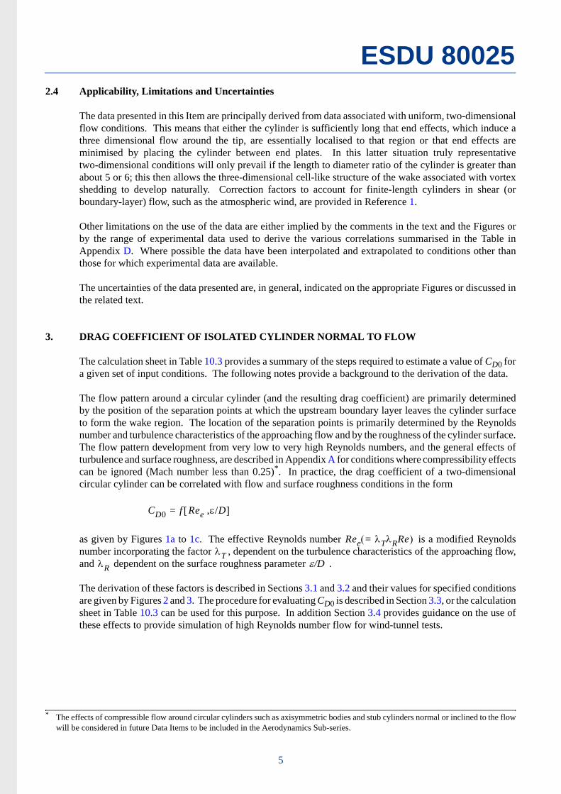

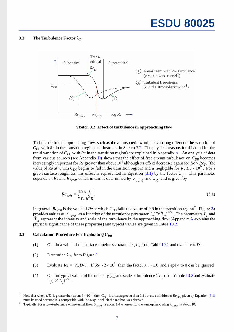


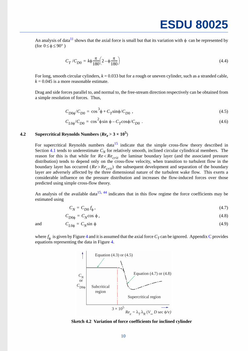
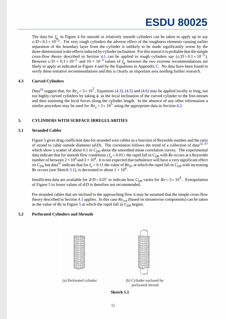


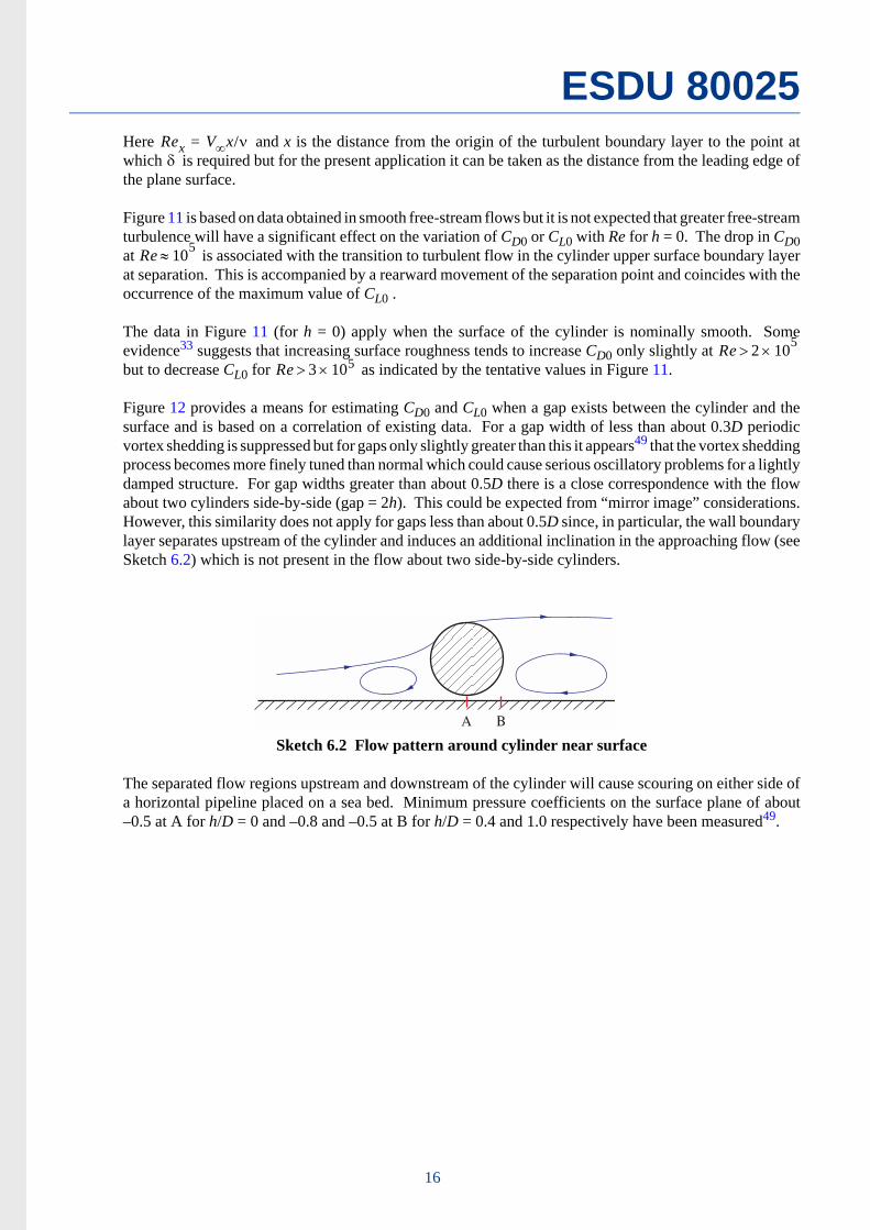

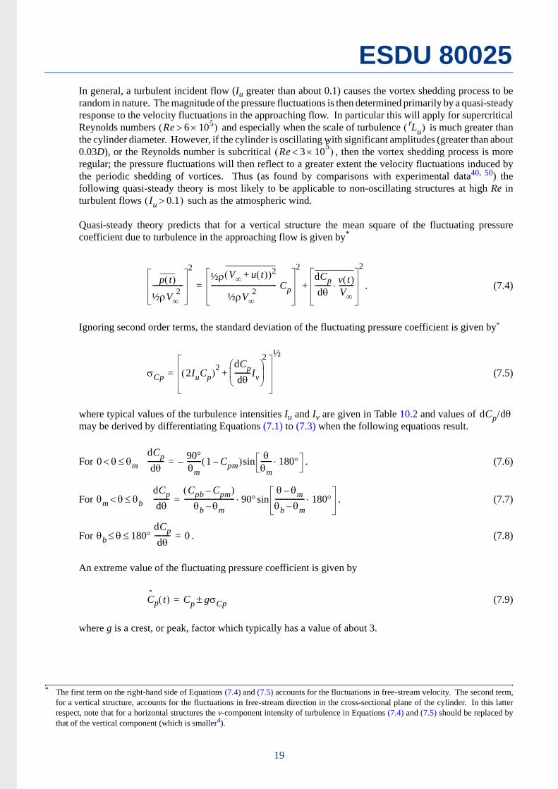


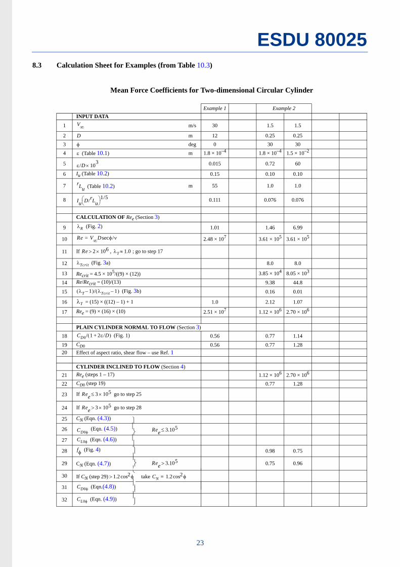


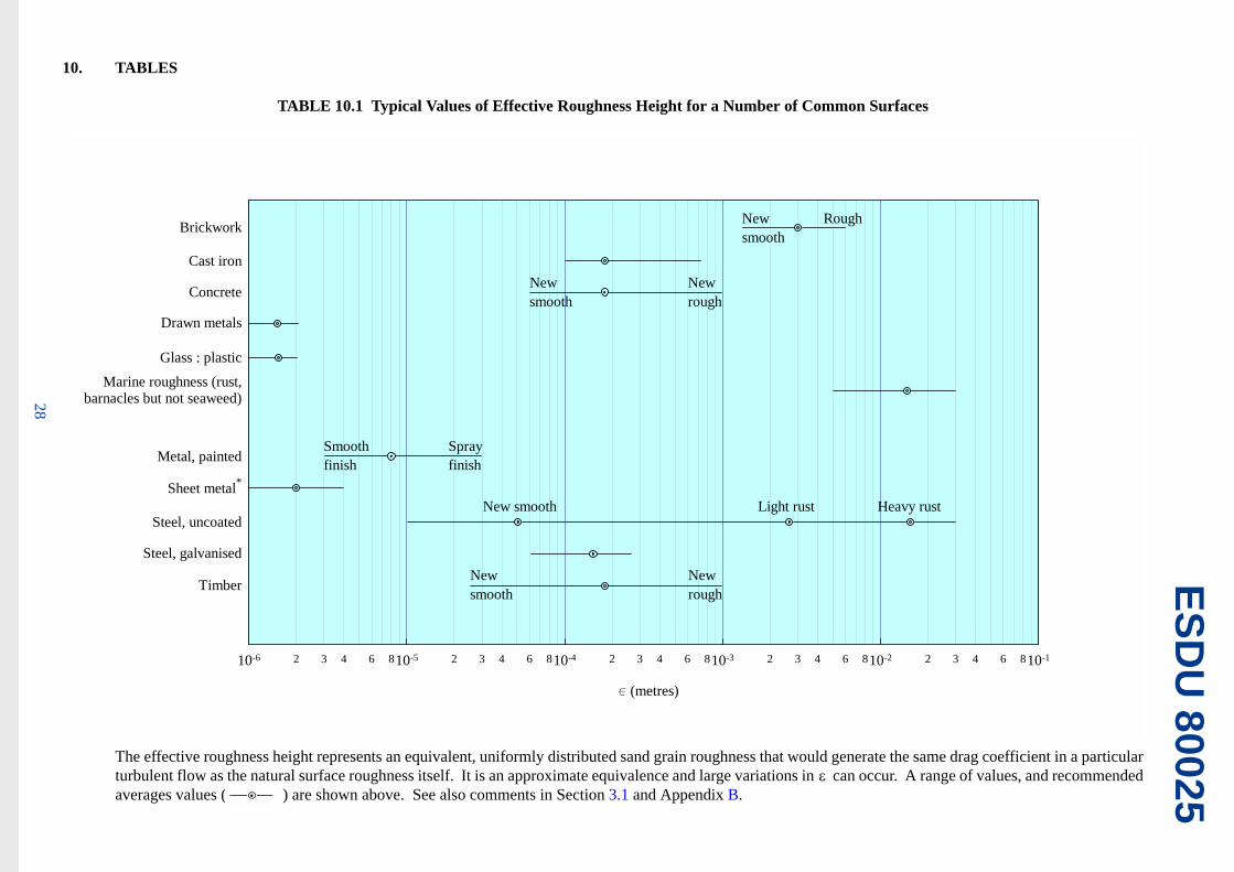

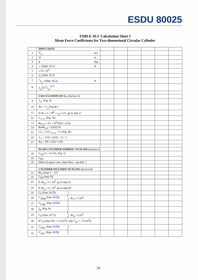


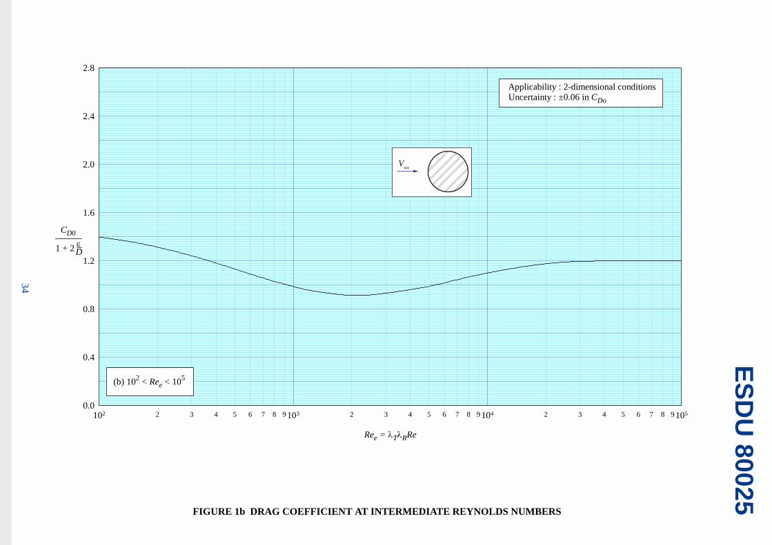
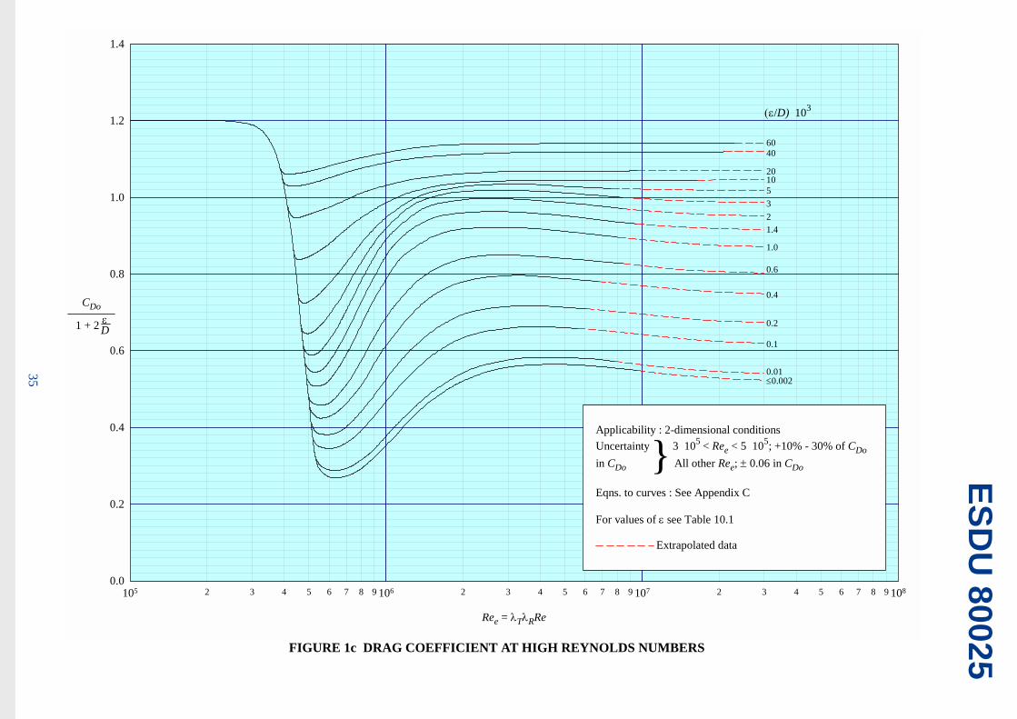
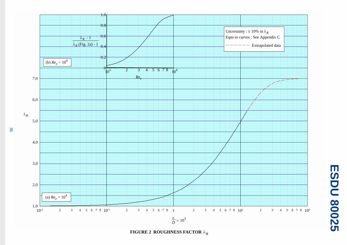
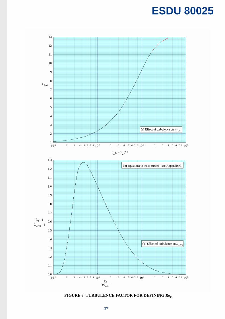

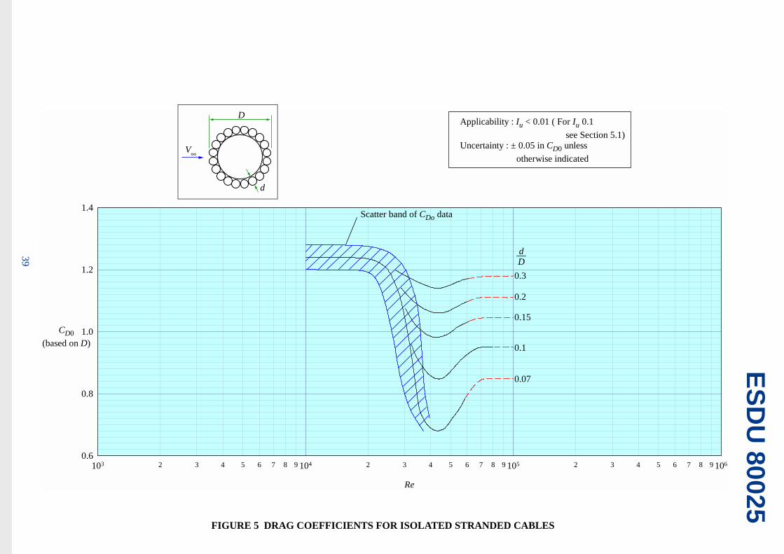


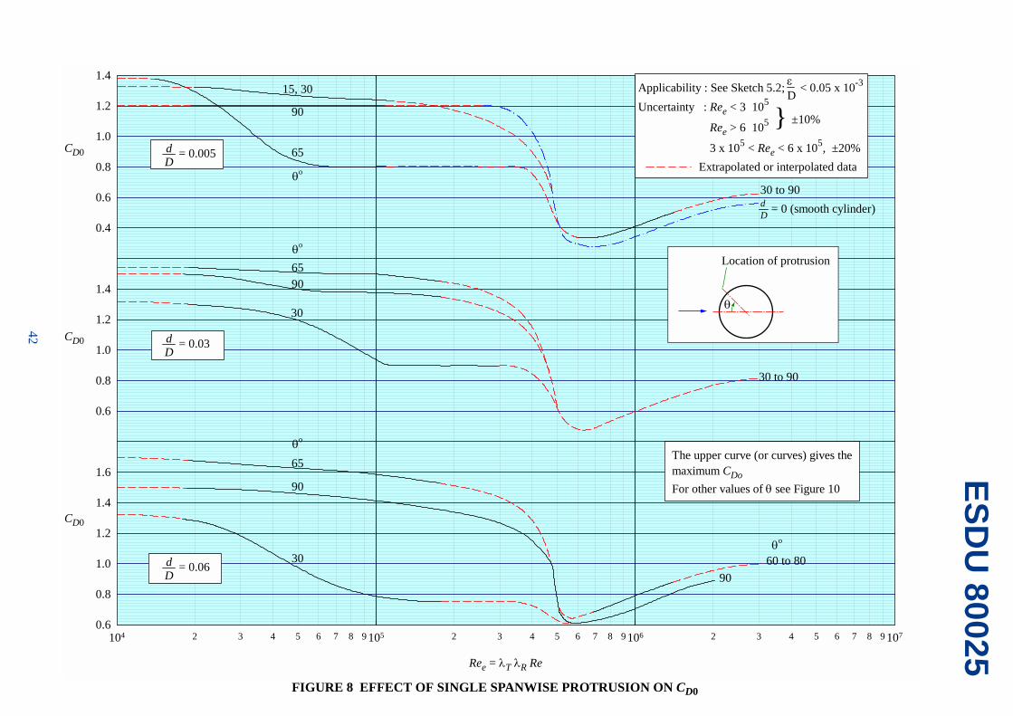


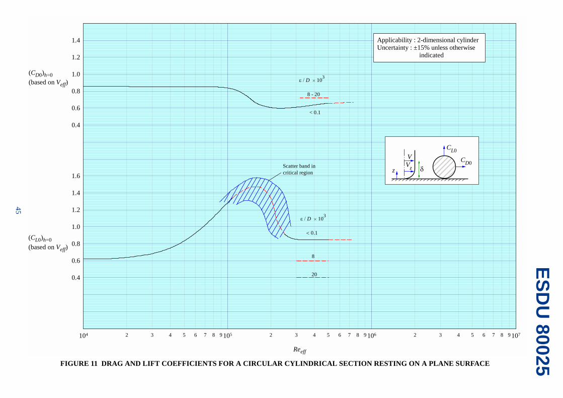
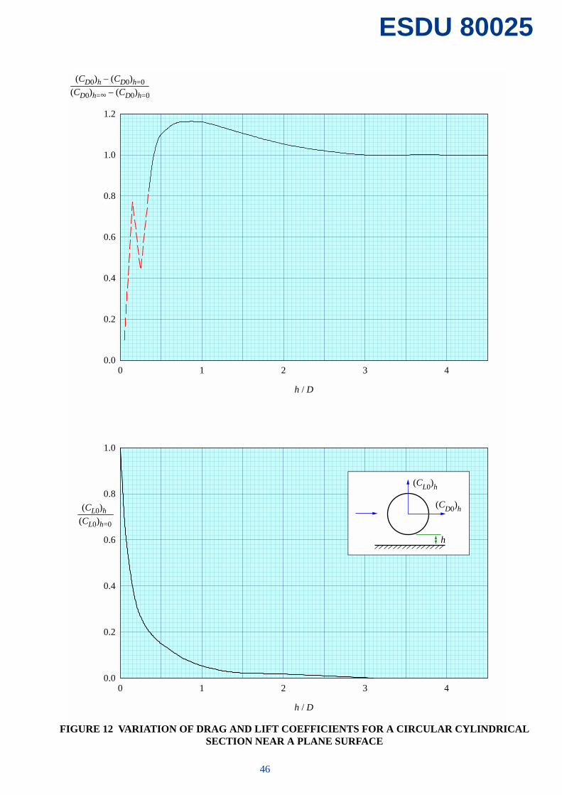


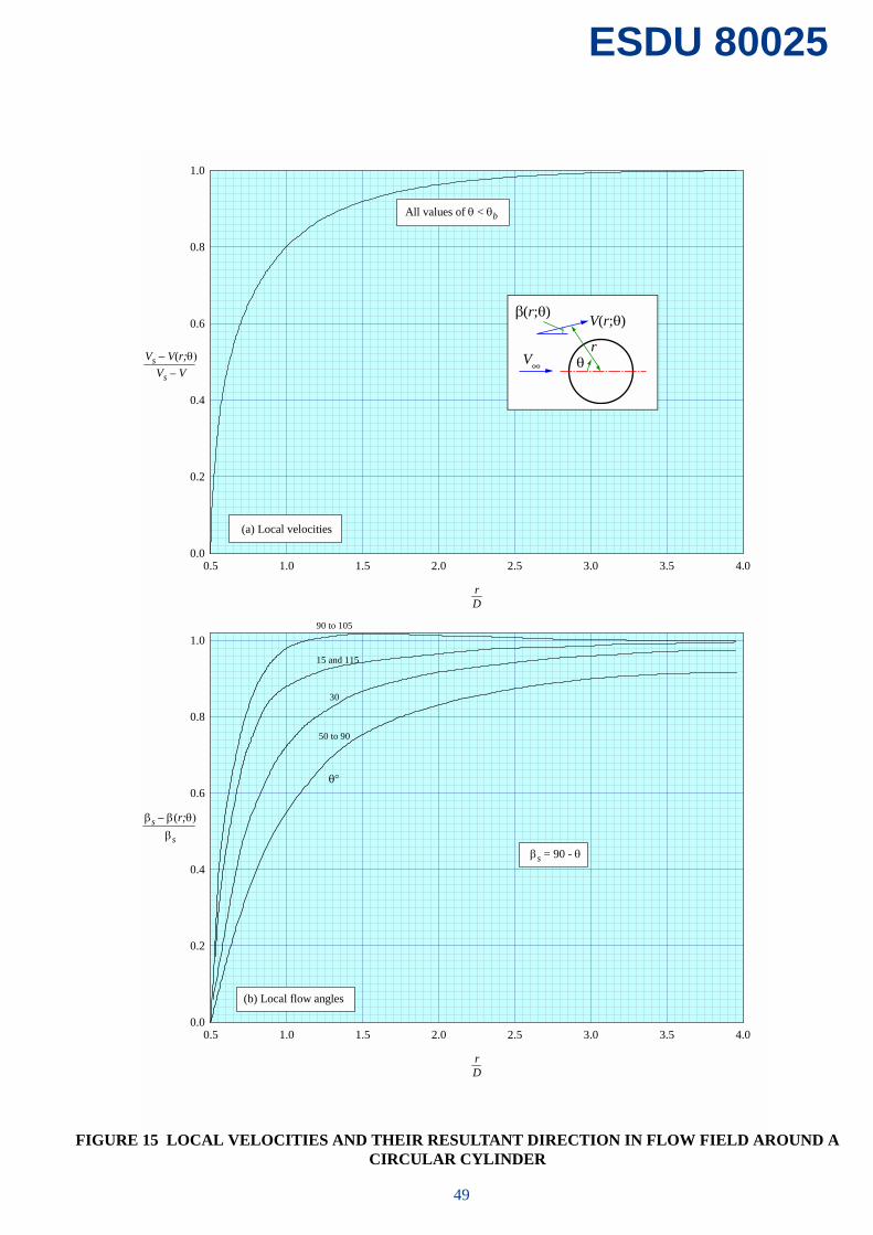

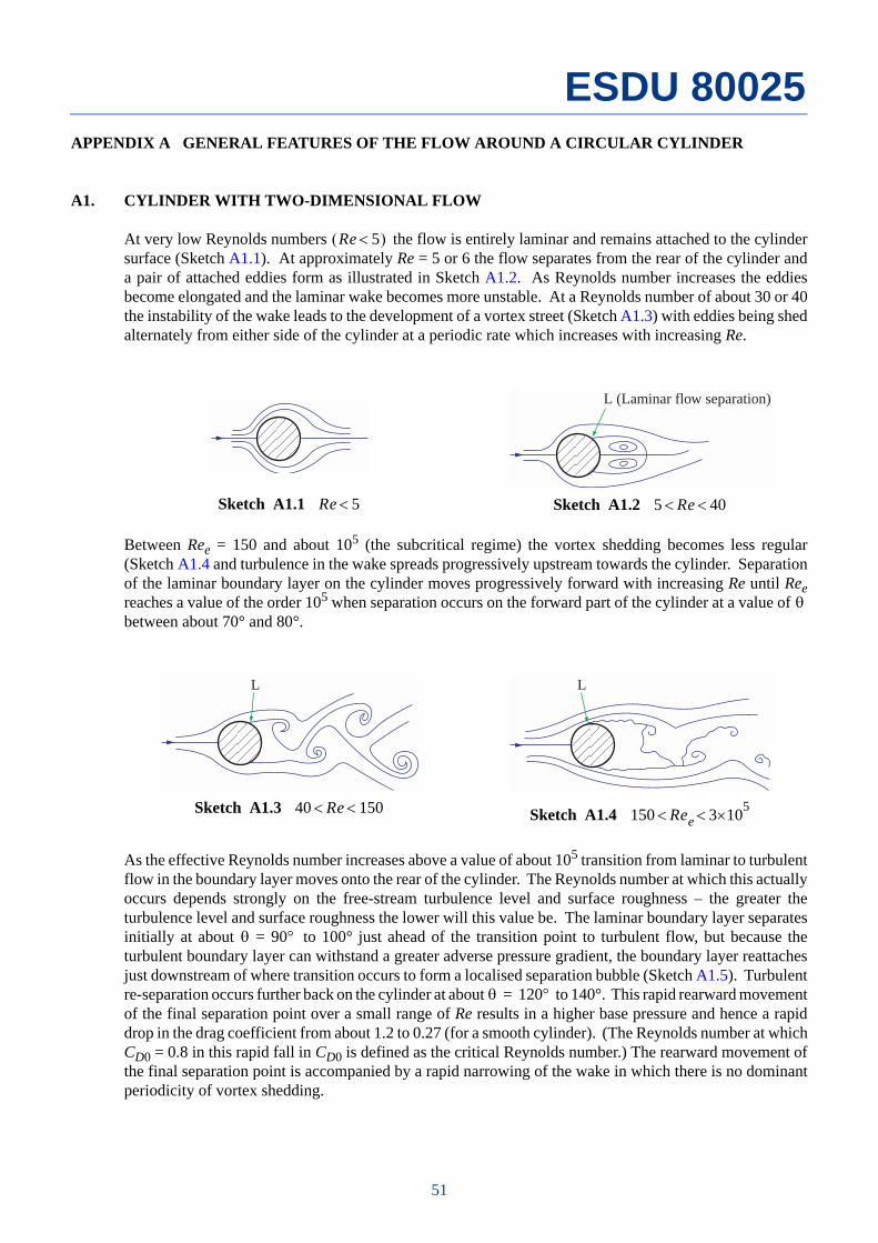


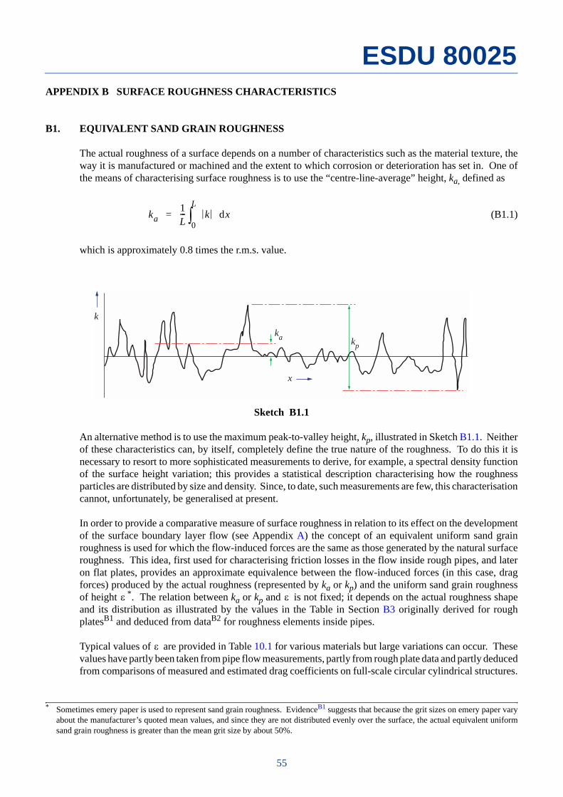


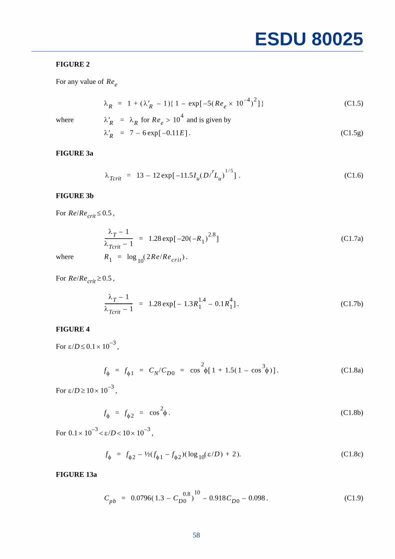


![THE ENVIRONMENT (PROTECTION) ACT, 1986jkdears.com/eers/pdf/Environment__Protection__ACT.pdf · 2010-01-05 · THE ENVIRONMENT (PROTECTION) ACT, 1986 (No. 29 of 1986) [23th May, 1986]](https://static.documents.pub/doc/80x56/5eaf4d819a5f751dc137fe9b/the-environment-protection-act-2010-01-05-the-environment-protection-act.jpg)


