ESI The Erwin Schr¨ odinger International Boltzmanngasse 9 Institute for Mathematical Physics A-1090 Wien, Austria Multi-Matrix Models and Tri-Sasaki Einstein Spaces Christopher P. Herzog Igor R. Klebanov Silviu S. Pufu Tiberiu Tesileanu Vienna, Preprint ESI 2271 (2010) November 26, 2010 Supported by the Austrian Federal Ministry of Education, Science and Culture Available online at http://www.esi.ac.at
Transcript
ESI The Erwin Schrodinger International Boltzmanngasse 9Institute for Mathematical Physics A-1090 Wien, Austria
Multi-Matrix Models andTri-Sasaki Einstein Spaces
Christopher P. Herzog
Igor R. Klebanov
Silviu S. Pufu
Tiberiu Tesileanu
Vienna, Preprint ESI 2271 (2010) November 26, 2010
Supported by the Austrian Federal Ministry of Education, Science and CultureAvailable online at http://www.esi.ac.at
PUPT-2359
Multi-Matrix Models and Tri-Sasaki Einstein
Spaces
Christopher P. Herzog,1 Igor R. Klebanov,1,2 Silviu S. Pufu,1
and Tiberiu Tesileanu1
Joseph Henry Laboratories1 and Center for Theoretical Science,2
Princeton University, Princeton, NJ 08544
Abstract
Localization methods reduce the path integrals in N ≥ 2 supersymmetric Chern-Simonsgauge theories on S3 to multi-matrix integrals. A recent evaluation of such a two-matrixintegral for the N = 6 superconformal U(N) × U(N) ABJM theory produced detailedagreement with the AdS/CFT correspondence, explaining in particular the N3/2 scaling ofthe free energy. We study a class of p-matrix integrals describing N = 3 superconformalU(N)p Chern-Simons gauge theories. We present a simple method that allows us to evaluatethe eigenvalue densities and the free energies in the large N limit keeping the Chern-Simonslevels ki fixed. The dual M-theory backgrounds are AdS4×Y , where Y are seven-dimensionaltri-Sasaki Einstein spaces specified by the ki. The gravitational free energy scales inverselywith the square root of the volume of Y . We find a general formula for the p-matrix freeenergies that agrees with the available results for volumes of the tri-Sasaki Einstein spacesY , thus providing a thorough test of the corresponding AdS4/CFT3 dualities. This formulais consistent with the Seiberg duality conjectured for Chern-Simons gauge theories.
November 2010
1 Introduction and Summary
The AdS/CFT correspondence [1–3] provides many predictions about the dynamics of strongly
interacting field theories in various numbers of dimensions. For the case of three dimensions,
ref. [4] predicted that the number of low-energy degrees of freedom on N coincident M2-
branes scales as N3/2 for large N . Remarkably, this surprising prediction was recently con-
firmed [5] in the context of the ABJM construction [6] of the U(N)k×U(N)−k Chern-Simons
gauge theory on coincident M2-branes. The paper [5] was in turn based on [7] where the
methods of localization [8] were shown to reduce the path integral of the Euclidean ABJM
theory on S3 to a matrix integral. This matrix model was solved in the large N limit with
N/k kept fixed [5, 9], leading to precise tests of the AdS/CFT correspondence for Wilson
loops and for the free energy (by which we mean minus the logarithm of the Euclidean par-
tition function). The exact solution of this matrix model is related by analytic continuation
to a solution [10] of another matrix model describing topological Chern-Simons theory on
S3/Z2; in particular, the formula for the resolvent has the same structure in the two cases.
A generalization of the matrix model to the case where the Chern-Simons levels do not add
up to zero was considered in [11].
The aim of our paper is to build on the major progress recently achieved in [5, 7, 9] in
several ways. In section 2 we revisit the matrix integral for the ABJM theory on S3 and
uncover the details of the eigenvalue distribution. The matrix eigenvalues are located along
the branch cuts of the resolvent used in [5] and derived in [10] for the S3/Z2 model. While
the endpoints of the cuts can be read off directly from the resolvent, the cuts themselves are
not simply parallel to the real axis, in contrast with the matrix model of [10]. In order to
gain intuition for the location of the eigenvalues, we develop a numerical method for finite
N and k. This method allows us to access values of N and k that are large enough for the
result to be a good approximation to the limit studied in [5,9]. Furthermore, we focus on the
limit where N is sent to infinity at fixed k where the ABJM model is expected to be dual to
the AdS4×S7/Zk background of M-theory. In this strong coupling limit we find analytically
that the structure of the solution simplifies considerably. An ansatz where the real parts
of the eigenvalues scale with√
N allows us to calculate the free energy analytically. Unlike
in [5], our method does not rely on resolvents or mirror symmetry. We confirm that the free
energy scales as N3/2 with the coefficient found in [5].
In section 3 we develop our analytic approach further and apply it to the large N limit
of matrix models describing quiver Chern-Simons gauge theories on S3. We study explicitly
a class of N = 3 superconformal U(N)p gauge theories with bifundamental matter, quartic
1
superpotentials, and Chern-Simons levels k1, k2, . . . , kp that sum to zero. These models were
introduced in [12] where their type IIB brane constructions were presented. The type IIB
brane constructions involve N D3-branes that are wrapped around a circle and intersect the
(1, q1), (1, q2), . . . , (1, qp) 5-branes located sequentially along the circle. The dual AdS4 × Y
M-theory backgrounds for these models, which involve certain seven-dimensional tri-Sasaki
Einstein spaces Y , were conjectured in [13]. The tri-Sasaki Einstein spaces Y are defined
to be bases of hyper-Kahler cones [14–16], and we take the Einstein metric on them to be
normalized so that Rmn = 6gmn. The p-matrix models for the gauge theories dual to AdS4×Y
may be read off from [7]. In the large N limit we calculate the eigenvalue densities for these
matrix models and show that they are piecewise linear. This remarkably simple conclusion
allows us to evaluate the coefficient of the N3/2 scaling of the free energy as a function
of the levels ki and compare it with the calculation on the gravity side of the AdS/CFT
correspondence [5,17]. For an arbitrary compact space Y we find that the gravitational free
energy is
F = N3/2
√
2π6
27 Vol(Y ). (1)
For p = 3 the tri-Sasaki Einstein spaces Y are the Eschenburg spaces [18] whose volumes
were determined explicitly in [19]. Our 3-matrix model free energy is in perfect agreement
with this volume formula.
Furthermore, we carry out calculations of the p-matrix model free energy and use them
to conjecture an explicit general formula for the volumes via the AdS/CFT correspondence.
For a general p-node quiver with CS levels ka = qa+1 − qa, with 1 ≤ a ≤ p and qp+1 = q1, we
conjecture in section 4 that
Vol(Y )
Vol(S7)=
∑
(V,E)∈T
∏
(a,b)∈E |qa − qb|∏p
a=1
[
∑pb=1 |qa − qb|
] , (2)
where the sum in the numerator is over the set T of all trees (acyclic connected graphs)
with p nodes. Such a tree (V, E) consists of the vertices V = {1, 2, . . . , p} and |E| = p − 1
edges. The volumes of the corresponding tri-Sasaki Einstein spaces Y had previously been
studied by Yee, who expressed them through an integral formula (eq. (3.49) of [20]). In
the cases we have checked, our formula (2) is consistent with that of [20]. Equation (2) is
invariant under permutations of the qa, supporting the conjectured Seiberg duality for Chern-
Simons theories with at least N = 2 supersymmetry [21–23], which may be motivated by
2
interchanging different types of 5-branes in the type IIB brane constructions of these models.
Recent work [5,7,24] and the present paper hint at a special role that may be played by
the Euclidean path integral of a 3-dimensional conformal field theory on S3. This quantity
may be analogous to the conformal anomaly coefficients in even dimensional CFT’s. Recall
that the anomaly coefficients are very useful measures of the number of degrees of freedom.
For even dimensional theories with weakly curved dual backgrounds, these coefficients can
be calculated using dual gravity in AdS space [25] leading to precise tests of the AdS/CFT
correspondence. Such a definition of the number of degrees of freedom is not available for
3-dimensional CFT’s. As mentioned already, the path integral on S3 can be reduced to
matrix integrals using supersymmetric localization methods [7]. Earlier work on gravity
in Euclidean AdS4 [17] has pointed to the usefulness of the corresponding quantity: after
adding certain surface counter-terms, the action becomes finite, I = π/(2GN), and appears
to be unambiguous. The successful matching of this finite gravitational action with the path
integral on S3 in [5] for the N = 6 ABJM theory, and in the present paper for a class of
N = 3 superconformal theories provides evidence for the usefulness of this quantity as a
measure of the number of degrees of freedom.
One may hope that the free energy on S3 is also a useful quantity for non-supersymmetric
fixed points.1 For example, one could aim to match the large N free energy on S3 for the
non-supersymmetric example of AdS/CFT correspondence conjectured for the O(N) sigma
model in three dimensions [26].
2 ABJM Matrix Model
2.1 Matrix Model Setup
As shown in [7], the partition function for ABJM theory on S3 localizes on configurations
where the auxiliary scalars σ and σ in the two N = 2 vector multiplets are constant N ×N
Hermitian matrices. Denoting the eigenvalues of σ and σ by λi and λi, with 1 ≤ i ≤ N , one
can write the partition function as
Z =1
(N !)2
∫
(
N∏
i=1
dλi dλi
(2π)2
)∏
i<j
(
2 sinhλi−λj
2
)2 (
2 sinhλi−λj
2
)2
∏
i,j
(
2 coshλi−λj
2
)2 exp
(
ik
4π
∑
i
(λ2i − λ2
i )
)
,
(3)
1Of course, another non-supersymmetric measure of the number of degrees of freedom, which is veryuseful physically, is the thermal free energy.
3
where k is the Chern-Simons level, and the precise normalization was chosen as in [5]. The
integration contour should be taken to be the real axis in each integration variable. When
the number N of eigenvalues is large, the integral in eq. (3) can be approximated in the
saddle point limit by Z = e−F , where the “free energy” F is an extremum of
F (λi, λi) = −ik
4π
∑
j
(λ2j − λ2
j) −∑
i<j
log
(
2 sinhλi − λj
2
)2(
2 sinhλi − λj
2
)2
+ 2∑
i,j
log
(
2 coshλi − λj
2
)
+ 2 log N ! + 2N log(2π)
(4)
with respect to λi and λi. The goal of this section is to compute the leading contribution to
F in such a large N expansion while holding k fixed.
Varying (4) with respect to λj and λj we obtain the saddle point equations:
−∂F
∂λi
=ik
2πλi −
∑
j 6=i
cothλj − λi
2+∑
j
tanhλj − λi
2= 0 ,
−∂F
∂λi
= − ik
2πλi −
∑
j 6=i
cothλj − λi
2+∑
j
tanhλj − λi
2= 0 .
(5)
Similar saddle point equations appear in the context of matrix models derived from topolog-
ical string theory [10,27], and can be solved using powerful techniques based on holomorphy
arguments and special geometry. Such methods were used in [5] to solve eqs. (5) in the limit
where N is taken to infinity while holding N/k fixed. Our goal in this paper is more modest
than solving the matrix model for any value of the ’t Hooft parameter N/k. We will work
at fixed k and take the large N/k limit. As we will see shortly, in such a limit we can find
the eigenvalue distribution using a more elementary approach.
2.2 A Numerical Solution
To gain intuition, one can start by solving the saddle point equations (5) numerically for
any values of N and k. One of the simplest ways to do so is to view the equations (5)
as describing the equilibrium configuration of 2N point particles whose 2-d coordinates are
given by the complex numbers λj and λj and that interact with the forces given by eq. (5).
This equilibrium configuration can be found by introducing a time dimension and writing
down equations of motion for λj(t) and λj(t) whose solution approaches the equilibrium
4
configuration (5) at late times in the same way as the solution to the heat equation approaches
a solution to the Laplace equation at late times. The equations of motion for the eigenvalues
are
τλdλi
dt= −∂F
∂λi
, τλ
dλi
dt= −∂F
∂λi
, (6)
where τλ and τλ are complex numbers that need to be chosen in such a way that the saddle
point we wish to find is an attractive fixed point as t → ∞.
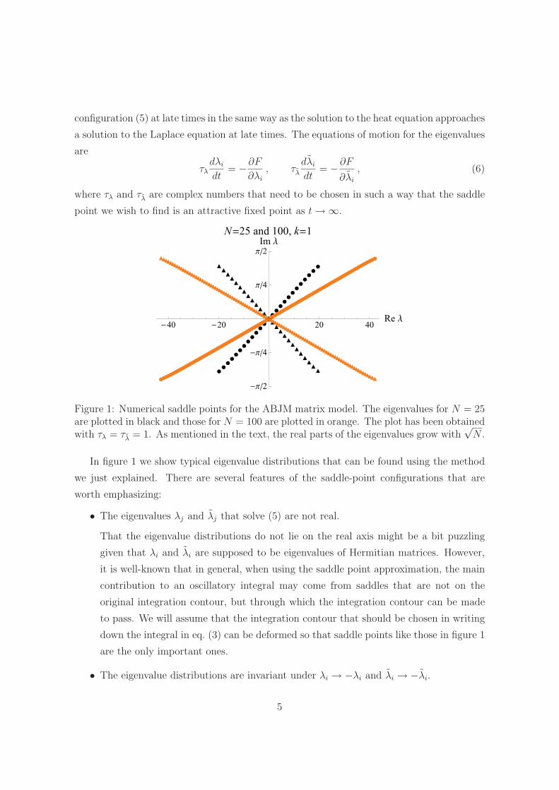
Figure 1: Numerical saddle points for the ABJM matrix model. The eigenvalues for N = 25are plotted in black and those for N = 100 are plotted in orange. The plot has been obtainedwith τλ = τλ = 1. As mentioned in the text, the real parts of the eigenvalues grow with
√N .
In figure 1 we show typical eigenvalue distributions that can be found using the method
we just explained. There are several features of the saddle-point configurations that are
worth emphasizing:
• The eigenvalues λj and λj that solve (5) are not real.
That the eigenvalue distributions do not lie on the real axis might be a bit puzzling
given that λi and λi are supposed to be eigenvalues of Hermitian matrices. However,
it is well-known that in general, when using the saddle point approximation, the main
contribution to an oscillatory integral may come from saddles that are not on the
original integration contour, but through which the integration contour can be made
to pass. We will assume that the integration contour that should be chosen in writing
down the integral in eq. (3) can be deformed so that saddle points like those in figure 1
are the only important ones.
• The eigenvalue distributions are invariant under λi → −λi and λi → −λi.
5
Indeed, the saddle point equations (5) are invariant under these transformations, so it
is reasonable to expect that there should be solutions that are also invariant.
• In the equilibrium configuration the two types of eigenvalues are complex conjugates
of each other, λj = λj.
Indeed, it is not hard to see that upon setting λj = λj the two equations in (5) become
equivalent, so it is consistent to look for solutions that have this property.
• As one increases N at fixed k, the imaginary part of the eigenvalues stays bounded
between −π/2 and π/2, while the real part grows with N . We will show shortly that
for the saddle points we find, the real part grows as N1/2 as N → ∞.
2.3 Large N Analytical Approximation
Let us now find analytically the solution to the saddle point equations (5) in the large N
limit. As explained above, we can assume λj = λj and write
λj = Nαxj + iyj , λj = Nαxj − iyj , (7)
where we introduced a factor of Nα multiplying the real part because we want xj and yj to
be of order one and become dense in the large N limit. The constant α is so far arbitrary
but will be determined later.
In passing to the continuum limit, we define the functions x, y : [0, 1] → R so that
xj = x(j/N) , yj = y(j/N) . (8)
Let us assume we order the eigenvalues in such a way that x is a strictly increasing function
on [0, 1]. Introducing the density of the real part of the eigenvalues
ρ(x) =ds
dx, (9)
one can approximate (4) as (see Appendix A)
F =k
πN1+α
∫
dx xρ(x)y(x) + N2−α
∫
dx ρ(x)2f(2y(x)) + · · · , (10)
6
where the function f is
f(t) = π2 −(
arg eit)2
. (11)
In other words, f is a periodic function with period π given by
f(t) = π2 − t2 when − π ≤ t ≤ π . (12)
It may be a little puzzling that while the discrete expression for the free energy in eq. (4)
is non-local, in the sense that there are long-range forces between the eigenvalues, its large N
limit (10) is manifestly local. One can understand this major simplification from examining,
for instance, the first saddle point equation in (5). The force felt by λi due to interactions
with far-away eigenvalues λj and λj is
− cothλj − λi
2+ tanh
λj − λi
2≈ − sgn(Re λj − Re λi) + sgn(Re λj − Re λi) , (13)
the corrections to this formula being exponentially suppressed in Reλj − Re λi and Re λj −Re λi. In other words, the non-local part of the interaction force between eigenvalues is
given just by the right-hand side of eq. (13). The non-local part of the force vanishes when
Re λj = Re λj, so in assuming that the two eigenvalue distributions are complex conjugates
of each other, we effectively arranged for an exact cancellation of non-local effects. All that
is left are short-range forces, which in the large N limit are described by the local action
(10).
One can view F as a functional of ρ(x) and y(x) and look for its saddle points in the set
C =
{
(ρ, y) :
∫
dx ρ(x) = 1; ρ(x) ≥ 0 pointwise
}
. (14)
These constraints mean that ρ is a normalized density. Motivated by the numerical analysis
we performed, we assume that ρ and y describe a connected distribution of eigenvalues
contained in a bounded region of the complex plane.
Let us assume a saddle point for F exists. As N → ∞, we need the two terms in (10) to
be of the same order in N in order to have non-trivial solutions, so from now on we will set
α =1
2. (15)
7
The real part of the eigenvalues therefore grows as N1/2, and to leading order, the free energy
behaves as N3/2 at large N . In writing (10) we omitted the last two terms from eq. (4).
They do not depend on ρ or y and hence do not affect the saddle point equations. They are
also lower order in N given the choice of α.
To find a saddle point for F , one can add a Lagrange multiplier µ to (10) and extremize
F = N3/2
[
k
π
∫
dx xρ(x)y(x) +
∫
dx ρ(x)2f(2y(x)) − µ
2π
(∫
dx ρ(x) − 1
)]
(16)
instead of (10). As long as ρ(x) > 0, the saddle point eigenvalue distribution satisfies the
equations
4πρ(x)f(2y(x)) = µ − 2kxy(x) ,
2πρ(x)f ′(2y(x)) = −kx .(17)
Plugging (12) into (17) one obtains
ρ(x) =µ
4π3, y(x) =
π2kx
2µ, (18)
as long as −π/2 ≤ y(x) ≤ π/2. If ρ is supported on [−x∗, x∗] for some x∗ > 0 that we will
determine shortly, we can calculate µ from the normalization of the density ρ(x):
∫ x∗
−x∗
dx ρ(x) = 1 =⇒ µ =2π3
x∗
. (19)
Plugging this formula back into (10), we obtain the free energy in terms of x∗:
F =N3/2(12π4 + k2x4
∗)
24π2x∗
+ o(N3/2) . (20)
This expression is extremized when
x∗ = π
√
2
k, y(x∗) =
π
2. (21)
Luckily, the answer y(x∗) = π/2 is consistent with our assumption that −π/2 ≤ y(x) ≤π/2 without which eq. (18) would not be correct. In Appendix B we check that assuming
y(x∗) > π/2 implies a contradiction. The extremum of F obtained from eqs. (20) and (21)
8
is
F =π√
2
3k1/2N3/2 + o(N3/2) . (22)
This result agrees with the free energy found in [5] using the regularized Euclidean action in
AdS4 [17].
-4 -2 2 4x
0.02
0.04
0.06
0.08
0.10
0.12
Ρ
N=200, k=1
Figure 2: Comparison between analytical prediction and numerical results for the density ofeigenvalues ρ defined in eq. (9). The dotted black line represents the analytical calculation,and the numerical result is shown in orange dots.
In the large N limit the eigenvalues therefore condense on two line segments and on these
two line segments they have uniform density. In figure 2 we compare the analytical result
for the density with the numerical one.
We would like to compare the location of our eigenvalue distributions with the results
of [5]. Noting a similarity between the ABJM matrix model and the S3/Z2 matrix model
solved in [10], Drukker, Marino, and Putrov [5] write down a resolvent for the ABJM model.
This resolvent has cuts in the λ plane corresponding to the locations of the eigenvalues. In
particular, it has a cut where the λi eigenvalues are located and a second cut where the λi
eigenvalues are located but shifted by πi. More specifically, the resolvent has the form
ω(λ) = 2 log
(
1
2
[
√
(eλ + b)(eλ + 1/b) −√
(eλ − a)(eλ − 1/a)]
)
. (23)
9
where a + 1/a + b + 1/b = 4 and at strong coupling,
a +1
a− b − 1
b= 2i exp
(
π
√
2N
k− 1
12
)
+ . . . (24)
The ellipses denote terms exponentially suppressed in N/k relative to the leading term.
Solving the equations for a and b, we find that the branch points in the λ plane are at
log a = π
√
2N
k− 1
12+
iπ
2, log
1
a= −π
√
2N
k− 1
12− iπ
2, (25)
log b = −π
√
2N
k− 1
12+
iπ
2, log
1
b= π
√
2N
k− 1
12− iπ
2. (26)
These expressions are in agreement with (21) in the large N limit.
We can also compute the 1/6 and 1/2 BPS Wilson loops in this strong coupling limit.
We have that [5, 28]
〈W 1/6�
〉 =2πiN
k
∫ x∗
−x∗
eλ(x)ρ(x)dx , (27)
〈W 1/2�
〉 =2πiN
k
∫ x∗
−x∗
(
eλ(x) + eλ(x))
ρ(x)dx . (28)
Plugging in our results, we find
〈W 1/6�
〉 ≈ −√
N
2keπ√
2N/k , (29)
〈W 1/2�
〉 ≈ i
2eπ√
2N/k . (30)
The exponents in these formulae agree with the results in [5, 28].
3 Necklace Quiver Gauge Theories
In this section we consider a class of quiver Chern-Simons U(N)k1×U(N)k2
× · · · ×U(N)kp
gauge theories whose quiver diagrams look like necklaces (see figure 3) [12,13]. In the N = 2
superspace formulation the theory is coupled to bi-fundamental chiral superfields Aa, Ba,
10
k1
k2
k3
k4
kp
Ap A1
A2
A3
B1
B2
B3
Bp
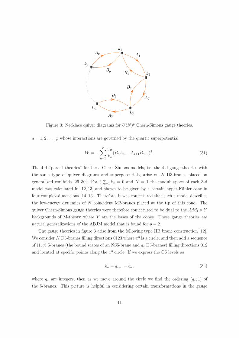
Figure 3: Necklace quiver diagrams for U(N)p Chern-Simons gauge theories.
a = 1, 2, . . . , p whose interactions are governed by the quartic superpotential
W = −p∑
a=1
2π
ka
(BaAa − Aa+1Ba+1)2 . (31)
The 4-d “parent theories” for these Chern-Simons models, i.e. the 4-d gauge theories with
the same type of quiver diagrams and superpotentials, arise on N D3-branes placed on
generalized conifolds [29, 30]. For∑p
a=1 ka = 0 and N = 1 the moduli space of each 3-d
model was calculated in [12, 13] and shown to be given by a certain hyper-Kahler cone in
four complex dimensions [14–16]. Therefore, it was conjectured that such a model describes
the low-energy dynamics of N coincident M2-branes placed at the tip of this cone. The
quiver Chern-Simons gauge theories were therefore conjectured to be dual to the AdS4 × Y
backgrounds of M-theory where Y are the bases of the cones. These gauge theories are
natural generalizations of the ABJM model that is found for p = 2.
The gauge theories in figure 3 arise from the following type IIB brane construction [12].
We consider N D3-branes filling directions 0123 where x3 is a circle, and then add a sequence
of (1, q) 5-branes (the bound states of an NS5-brane and qa D5-branes) filling directions 012
and located at specific points along the x3 circle. If we express the CS levels as
ka = qa+1 − qa , (32)
where qa are integers, then as we move around the circle we find the ordering (qa, 1) of
the 5-branes. This picture is helpful in considering certain transformations in the gauge
11
theory that are analogous to the Seiberg duality in four-dimensional gauge theory [21–23].
As in that case, these transformations are related to interchange of adjacent branes and thus
correspond to interchange of qa and qa+1. (There is also a shift in the rank of one of the
gauge groups that may be neglected in the large N limit.) Our explicit answer for the free
energy will have this symmetry.
For a general set of Chern-Simons levels such a p > 2 gauge theory has N = 3 superconfor-
mal invariance, but in the special case where p is even and the CS levels are (k,−k, k,−k, . . .)
the supersymmetry is enhanced to N = 4 [12, 31, 32]. Then Y = S7/(Zp/2 × Zkp/2) and
Vol(Y ) = 4π4/(3kp2). For more general ki the eight-dimensional cone is not an orbifold,
which complicates the calculation of its volume. Nevertheless, these volumes were computed
in [19,20], and we can compare the result on the gravity side with our calculation of the free
energy.
3.1 Multi-Matrix Models
As explained in [7], the partition function for the necklace quivers in figure 3 localizes on
configurations where the scalars σa in the N = 2 vector multiplets are constant Hermitian
matrices. Denoting by λa,i, 1 ≤ i ≤ N , the eigenvalues of σa, the partition function takes
the form of the matrix integral
Z =1
(N !)p
∫
(
∏
a,i
dλa,i
2π
)
p∏
a=1
∏
i<j
(
2 sinhλa,i−λa,j
2
)2
∏
i,j 2 coshλa,i−λa+1,j
2
exp
[
i
4π
∑
i
kaλ2a,i
]
. (33)
The normalization of the partition function was chosen so that it agrees with the ABJM
result from eq. (3) in the case p = 2. As in the ABJM case, the integration contour should
be taken to be the real axis in each integration variable. The saddle point equations following
from (33) are
ika
πλa,i − 2
∑
j 6=i
cothλa,j − λa,i
2+∑
j
tanhλa+1,j − λa,i
2+∑
j
tanhλa−1,j − λa,i
2= 0 . (34)
These equations can be solved numerically using the method described in section 2.2: by
replacing the right-hand side of these equations by τadλa,j/dt, we obtain a system of first
order differential equations whose solution converges at late times t to a solution of eq. (34)
provided that the constants τa are chosen appropriately. We will now show how to obtain
an approximate analytical solution valid in the limit where N is taken to be large and k is
12
held fixed.
Based on our intuition from the ABJM model, let us assume that in this case too the
real part of the eigenvalues behaves as N1/2 at large N while the imaginary part is of order
one. So if one writes
λa,j = N1/2xa,j + iya,j , (35)
then the quantities xa,j and ya,j become dense in the large N limit. Under this assumption,
we will be able to solve the saddle point equations to leading order in N in a self-consistent
way. We can pass to the continuum limit by considering the normalized densities ρa(x) of
the xa,j together with the continuous functions ya(x) that describe the imaginary parts of
the eigenvalues as functions of x. Let us first make a rough approximation to the saddle
point equations (34). When N is large, we have
cothλa,j − λa,i
2≈ sgn (xa,j − xa,i) , tanh
λa,j − λa±1,i
2≈ sgn (xa,j − xa±1,i) . (36)
To leading order in N , the saddle point equations then become
∫
dx′ [2ρa(x′) − ρa+1(x
′) − ρa−1(x′)] sgn(x′ − x) = 0 . (37)
Differentiating with respect to x, we immediately conclude that all ρa must be equal to one
another to leading order in N , so we can write ρa(x) ≡ ρ(x) for some density function ρ(x)
that is normalized as
∫
dx ρ(x) = 1 . (38)
With the simplifying assumption that the densities ρa are equal, one can go back to the
integral (33) and calculate the free energy functional F [ρ, ya] to leading order in N (see
Appendix A):
F [ρ, ya] =N3/2
2π
∫
dx xρ(x)
p∑
a=1
kaya(x)
+N3/2
2
∫
dx ρ(x)2
p∑
a=1
f(ya+1(x) − ya(x)) + o(N3/2) ,
(39)
where f is the same function that was defined in (11). We wish to evaluate the integral
13
(33) in the saddle point approximation where it equals Z = e−F , the free energy F being
an appropriate critical point of F [ρ, ya]. Let us assume that the eigenvalue distribution
corresponding to this saddle point is connected, symmetric about x = y = 0, and bounded.
In looking for the eigenvalue distribution that extremizes (39) to order O(N3/2), an
important observation is that, in fact, one cannot find this distribution, because to this
order in N F [ρ, ya] has a flat direction given by ya(x) → ya(x) + δy(x) for any function
δy(x). The second term in eq. (39) is clearly invariant under this transformation, and the
first term is also invariant because∑p
a=1 ka = 0. The existence of this flat direction is not
a problem at all if one just wants to compute the free energy F to leading order in N . If
one’s goal is instead to find the eigenvalue distributions for the saddle point, subleading
corrections to (39) that presumably lift this flat direction must be taken into account. In
this paper we will content ourselves with calculating the free energy to order O(N3/2), and
will leave a careful analysis of how the flat direction gets lifted for future work.
Before we examine the extremization of the free energy functional (39) in more detail,
let us make a few comments and present a result that follows already from the discussion
above. Suppose we manage to find a saddle point of F by extremizing (39) for a quiver
Chern-Simons gauge theory that in the large N limit and at strong ’t Hooft coupling is dual
to an AdS4 × Y M-theory background. Let us assume that this saddle point gives the most
important contribution to the partition function. What can we learn? From (39) one may
infer that the free energy grows as N3/2 at large N as expected from supergravity, so our
computation provides a gauge theory explanation of this N3/2 behavior. Moreover, one can
compare the free energy we obtain with the exact M-theory result
F = N3/2
√
2π6
27 Vol(Y )(40)
that can be derived as a straightforward generalization of the ABJM computation in [5]. Via
this formula we will compare successfully our matrix model results with the expressions for
the volumes of tri-Sasaki Einstein space available in the literature [19,20].
3.2 A Class of Orbifold Chern-Simons Theories
The vacuum moduli space of the non-chiral quivers with alternating CS levels (k,−k, k,−k, . . .)
and N = 1 is the orbifold C4/(
Zp/2 × Zkp/2
)
[12]. There is an induced orbifold action on
the unit 7-sphere in C4, and thus the internal space Y is S7/
(
Zp/2 × Zkp/2
)
. Consequently,
14
we expect
Vol(Y ) =4 Vol(S7)
kp2=
4π4
3kp2, (41)
where in the second equality we used the round 7-sphere volume Vol(S7) = π4/3.
This formula can be reproduced very easily from the matrix model computation. The
saddle point equations (34) are solved by setting λ2a,i = λi and λ2a+1,i = λi, λi and λi
being the eigenvalues for the saddle point of the ABJM matrix model discussed in detail in
section 2. The free energy of the p-node quiver with CS levels (k,−k, k,−k, . . .) is therefore
p/2 times the free energy in the ABJM model, and thus
F =p
2FABJM =
π√
2
6pk1/2N3/2 + o(N3/2) . (42)
Using eq. (40), one immediately reproduces the volume of the S7-orbifold in eq. (41).
3.3 Warm-up: A Four-Node Quiver
k1 = k k2 = k
k4 = −k k3 = −k
Figure 4: Four-node quiver diagram obtained as a particular case of the general quiverspresented in figure 3.
Another case we can easily solve using the approximation scheme developed above is
that of the four-node quiver with CS levels ka = (k, k,−k,−k) (see figure 4). The two Z2
symmetries of the quiver, one acting by interchanging nodes 1 ↔ 4 and 2 ↔ 3 and the other
by interchanging nodes 1 ↔ 2 and 3 ↔ 4, allow us to set
λ1,j = λ2,j = λj , λ3,j = λ4,j = λj . (43)
15
Moreover, in the saddle point equations (34) it is consistent to set λj = λj as in the ABJM
case, which reduces our task to finding a single eigenvalue distribution λi. In passing to the
continuum limit, we should therefore set
y1 = y2 = −y3 = −y4 = y . (44)
The free energy functional (39) then becomes
F [ρ, y] =2kN3/2
π
∫
dx xρ(x)y(x) + N3/2
∫
dx ρ(x)2[
π2 + f(2y(x))]
+ o(N3/2) . (45)
In the paragraph following eq. (39) we discussed how for arbitrary p-node quivers we
would not be able to solve for the ya themselves, but only for differences of consecutive ya,
because the leading large N contribution to the free energy functional is invariant under the
shifts ya → ya + δy for any function δy. In the case of the (k, k,−k,−k) quiver we will,
however, be able to determine the location of the eigenvalues exactly, because the ansatz
(44) breaks this shift symmetry.
In order to find the saddle points of (45) in the set (14), we should add a Lagrange
multiplier µ to enforce the normalization condition for ρ, and extremize the functional
F [ρ, y] = F − N3/2
2πµ
(∫
dx ρ(x) − 1
)
. (46)
Let us assume the eigenvalue distribution is symmetric around x = y = 0 and ranges
between [−x∗, x∗]. Let us focus on the region where x ≥ 0. Solving the equations of motion
we obtain
ρ(x) =µ
8π3, y(x) =
2kπ2x
µ, if − π
2≤ y(x) <
π
2. (47)
Since ρ(x) > 0 in this region, we have µ > 0 and y(x) ≥ 0. Assuming y(x∗) < π/2, we can
find µ in terms of x∗ from the normalization condition for ρ, and then express F in terms
of x∗ and extremize it. The extremization yields x∗ = 21/4π/√
k and y(x∗) = π/√
2 > π/2,
which suggests that the assumption y(x∗) < π/2 might be wrong. One could imagine that
y(x∗) > π/2, but solving the saddle point equations in the region where y > π/2 would yield
ρ(x) < 0.
The correct answer is y(x∗) = π/2, and in fact y(x) = π/2 on some interval [xπ/2, x∗]
16
with 0 < xπ/2 < x∗. On this interval,
ρ(x) =µ − 2kπx
4π3, y(x) =
π
2, (48)
where in obtaining these equations we only varied (46) with respect to ρ. The quantity xπ/2
can be obtained from setting y(xπ/2) = π/2 in (47):
xπ/2 =µ
4πk. (49)
One can now find µ by imposing the normalization condition for ρ, and then express the free
energy F in terms of x∗ and extremize with respect to x∗. The result is that
x∗ = 2xπ/2 = 2π
√
2
3k, µ = 4π2
√
2k
3. (50)
The density of eigenvalues is constant on [−xπ/2, xπ/2] and then drops linearly to zero on
Figure 5: Comparison between numerics and analytical prediction for the four-node quiverwith k = {1, 1,−1,−1}. The dotted black lines represent the large N analytical predictionand the orange dots represent numerical results.
[−x∗,−xπ/2] and [xπ/2, x∗]. See figure 5 for a comparison of this analytical prediction with a
numerical solution of the saddle point equations.
The free energy for this model can be computed from (45):
F =
√
32
27πk1/2N3/2 + o(N3/2) . (51)
Using (40), we infer that the gravity dual of the Chern-Simons quiver gauge theory with CS
17
levels (k, k,−k,−k) is AdS4 × Y where the volume of the compact space Y is
Vol(Y ) =π4
16k. (52)
Satisfyingly, this result is in agreement with the calculation of the corresponding integral
representation given in [20] for k = 1, which we will review in section 4.
k1 = k k2 = k
k4 = −k k3 = −k
Figure 6: The Chern-Simons quiver gauge theory dual to AdS4 × Q2,2,2/Zk as proposedin [33,34].
Let us also note that this volume is the same as that of a Zk orbifold of the Sasaki-
Einstein space Q2,2,2, which in turn is a Z2 orbifold of the coset space SU(2) × SU(2) ×SU(2)/ (U(1) × U(1)). If we denote the generators of the three SU(2) factors by ~JA, ~JB,
and ~JC , then the two U(1) groups we are modding out by are generated by JA3 + JB3 and
JA3 +JC3. Q2,2,2 admits a toric Sasaki-Einstein metric, and a proposal for the Chern-Simons
quiver gauge theory dual to AdS4 × Q2,2,2/Zk was made in [33, 34]. This proposal is quite
similar to the (k, k,−k,−k) non-chiral quiver in figure 4, except it is chiral—see figure 6.
Due to the chiral nature of the quiver, the corresponding matrix model that follows from [7]
is somewhat different. Its analysis is beyond the scope of this paper.
3.4 Extremization of the Free Energy Functional and Symmetries
Since the free energy functional (39) depends only on differences between consecutive ya, we
find it convenient to introduce the notation δya = ya−1 − ya and to write ka = qa+1 − qa as
in eq. (32). Equation (39) becomes
F [ρ, δya] =N3/2
2π
∫
dx xρ(x)
p∑
a=1
qaδya(x) +N3/2
2
∫
dx ρ(x)2
p∑
a=1
f(δya(x)) + o(N3/2) . (53)
18
This expression should be extremized over the set
C =
{
(ρ, δya) :
∫
dx ρ(x) = 1; ρ(x) ≥ 0 and
p∑
a=1
δya(x) = 0 pointwise
}
. (54)
Since∑p
a=1 δya = 0, one could either use this constraint to solve for one of the δya and
extremize (53) only with respect to the remaining ones, or, as we will do, one could introduce
a Lagrange multiplier ν(x) that enforces the constraint and treat all δya on equal footing.
Because of the normalization constraint (38) we also need a Lagrange multiplier µ. We
therefore will extremize
F [ρ, δya] = F [ρ, δya] −N3/2
2πµ
(∫
dx ρ(x) − 1
)
− N3/2
2π
∫
dx ρ(x)ν(x)
p∑
a=1
δya(x) (55)
instead of (53). Suppose a saddle point exists. As long as ρ(x) > 0, the saddle point
eigenvalue distribution should satisfy the equations
Figure 7: Comparison between numerics and analytical results for a three node quiver. Thedotted black lines represent the analytical large N approximation, while the orange dotsrepresent numerical results.
The normalization condition on ρ yields
µ = π2
√
18q1(q1 + q2)(2q1 + q2)
q22 − 5q2
1 − 5q1q2
= π2
√
2(k1 + k2)(k2 − k3)(k1 − k3)
(k1k2 − k1k3 − k2k3). (59)
Performing the integral (39), one obtains
F =N3/2µ
3π=
N3/2π√
2
3
√
(k1 + k2)(k2 − k3)(k1 − k3)
k1k2 − k1k3 − k2k3
. (60)
Given the free energy in the case k3 < 0 < k1 ≤ k2, it is actually possible to compute
the free energy for any 3-node quivers. Indeed, since in the case where there are only three
nodes a permutation of the ka can be thought of as a relabeling of the nodes, the free
energy must be invariant under all such permutations. In addition, the free energy must be
invariant under sending ka → −ka according to the second discrete symmetry discussed at
the end of section 3.4. Combining these two properties, one can find the free energy of an
arbitrary quiver with CS levels ka by constructing the new CS levels k1 = min(|k1| , |k2| , |k3|),k3 = −max(|k1| , |k2| , |k3|), and k2 = −k1 − k3 that satisfy k3 < 0 < k1 ≤ k2 and for which
eq. (60) holds. The unique extension of (60) that gives the correct answer for arbitrary CS
We can also compute the leading large N contribution to the free energy for arbitrary 4-node
quivers. Let us first examine the case where q4 ≥ q2 ≥ q1 ≥ q3 and |q4| is the largest among
the qa. It is convenient to require∑4
a=1 qa = 0 since many of the intermediate formulae
simplify under this assumption. Then we have q4 > 0 ≥ q1 ≥ q3 and |q4| ≥ |q3| ≥ |q1| ≥ |q2|.As in the three-node case, the solution to eqs. (56) breaks into three regions:
0 ≤ x ≤ µ
4πq4
: (64a)
δya =4π2xqa
µ, ρ =
µ
8π3,
µ
4πq4
≤ x ≤ − µ
4πq3
: (64b)
δy1 =(3q1 + q4)x
6πρ− π
3, δy2 =
(3q2 + q4)x
6πρ− π
3,
δy3 =(3q3 + q4)x
6πρ− π
3, δy4 = π , ρ =
3µ − 4πq4x
16π3,
− µ
4πq3
≤ x ≤ µ
2π(q2 + q4): (64c)
δy1 =(q1 − q2)x
4πρ, δy2 =
(q2 − q1)x
4πρ,
δy3 = −π , δy4 = π , ρ =µ + (q3 − q4)πx
4π3.
The first region ends where δy4 reaches π. At this endpoint |δya| = π |qa| / |q4| ≤ π for
Figure 8: Comparison between numerics and analytical results for a four node quiver. Thedotted black lines represent the analytical large N approximation, while the orange dotsrepresent numerical results.
a = 1, 2, 3. The second region ends where δy3 = −π. At this endpoint δy1 = π(q1 −q2)/(q1 + q2 − 2q3), and since q1 ≥ q3 and q2 ≥ q3, by the triangle inequality it follows that
|q1 − q2| ≤ q1 + q2 − 2q3, so |δy1| ≤ π. Similarly, |δy2| ≤ π also. Lastly, if q2 = q1 the third
region does not exist. When q2 > q1 and q1 < 0, δy1 is monotonically decreasing and δy2
is monotonically increasing in the third region, and this region ends where δy1 = −π and
δy2 = π. See figure 8 for an example.
From∫
dx ρ(x) = 1, one can find that µ is given by
8π2
µ=
√
1
q3
− 1
q4
+4(q2 + q3)
(q2 + q4)2+
12
q2 + q4
. (65)
The free energy is
F =N3/2µ
3π=
8πN3/2
3
(
1
q3
− 1
q4
+4(q2 + q3)
(q2 + q4)2+
12
q2 + q4
)−1/2
. (66)
Given eq. (66), one can use the symmetries we discussed at the end of section 3.4 to
compute the free energy of a quiver gauge theory with arbitrary qa. Indeed, one can define
qa to be a permutation of the four numbers qa − 14
∑4b=1 qb that gives |q4| ≥ |q3| ≥ |q1| ≥ |q2|.
If q4 is negative, one should flip the sign of all qa, so we can assume q4 > 0. By construction,
the qa sum to zero, so the second and third largest in absolute value, namely q3 and q1, are
negative. Therefore, the qa satisfy all the assumptions under which eq. (66) was derived,
and since the free energy does not change in going from qa to qa, one can plug the qa into
eq. (66) to find the free energy of an arbitrary 4-node quiver theory. The unique extension
23
of (66) to arbitrary qa can also be written as
F =N3/2π
√2
3
√
∏4a=1
(∑4
b=1 |qab|)
∑
(a,b) 6=(c,d) 6=(e,f) |qab| |qcd| |qef | −∑
(a,b,c) |qab| |qbc| |qca|, (67)
where qab denotes qa − qb, and in the denominator the first sum is over distinct unordered
pairs of numbers from 1 to 4 while the second sum is over unordered triplets. Using eq. (40),
we obtain a prediction for the volume of the compact space Y :
Vol(Y )
Vol(S7)=
∑
(a,b) 6=(c,d) 6=(e,f) |qab| |qcd| |qef | −∑
(a,b,c) |qab| |qbc| |qca|∏4
a=1
(∑4
b=1 |qab|) . (68)
4 A General Formula and its Tests
Equations (67) and (68) suggest a generalization to arbitrary p-node quivers. Note first that
the numerator of eq. (68) is a sum over all possible graphs with 4 nodes and 3 edges from
which we subtract the sum over all cyclic graphs with 4 nodes and 3 edges, yielding a sum
over all possible trees.
We conjecture that for a p-node quiver, the volume of the tri-Sasaki Einstein space Y
(normalized so that Rmn = 6gmn) is given by
Vol(Y )
Vol(S7)=
∑
(V,E)∈T
∏
(a,b)∈E |qa − qb|∏p
a=1
[
∑pb=1 |qa − qb|
] , (69)
where T is the set of all trees (acyclic connected graphs) with nodes V = {1, 2, . . . , p} and
A standard result in graph theory states that trees with p nodes have p − 1 edges.
The conjecture in eq. (69) is consistent with the results from 2, 3, and 4-node quivers,
and we also checked it for 5 and 6-node quivers. This formula is invariant under all the
symmetries discussed at the end of section 3.4. In particular, a quite non-trivial check of our
approach is that this formula is invariant under the Seiberg dualities described in [21–23].
The connection we observe between large N matrix integrals and sums over the tree graphs
is reminiscent of the connection between matrix models for 2-d quantum gravity and the
Kontsevich matrix model which generates ribbon graphs [35].
24
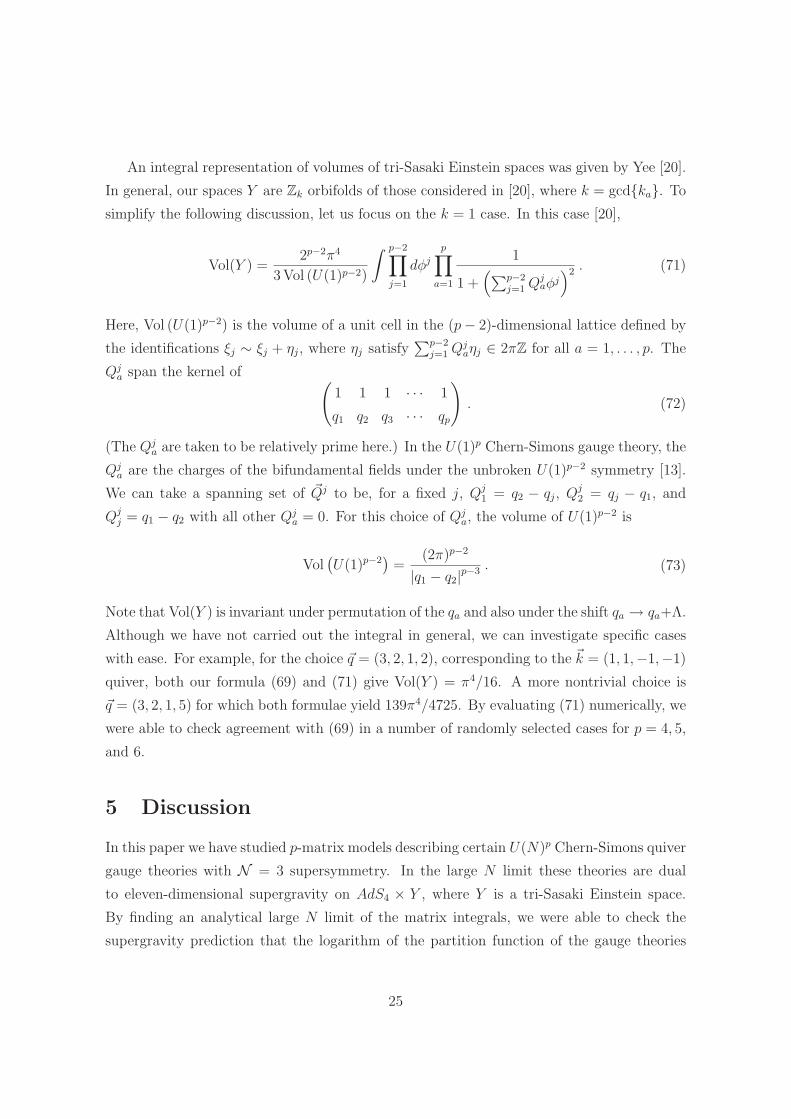
An integral representation of volumes of tri-Sasaki Einstein spaces was given by Yee [20].
In general, our spaces Y are Zk orbifolds of those considered in [20], where k = gcd{ka}. To
simplify the following discussion, let us focus on the k = 1 case. In this case [20],
Vol(Y ) =2p−2π4
3 Vol (U(1)p−2)
∫ p−2∏
j=1
dφj
p∏
a=1
1
1 +(
∑p−2j=1 Qj
aφj)2 . (71)
Here, Vol (U(1)p−2) is the volume of a unit cell in the (p − 2)-dimensional lattice defined by
the identifications ξj ∼ ξj + ηj, where ηj satisfy∑p−2
j=1 Qjaηj ∈ 2πZ for all a = 1, . . . , p. The
Qja span the kernel of
(
1 1 1 · · · 1
q1 q2 q3 · · · qp
)
. (72)
(The Qja are taken to be relatively prime here.) In the U(1)p Chern-Simons gauge theory, the
Qja are the charges of the bifundamental fields under the unbroken U(1)p−2 symmetry [13].
We can take a spanning set of ~Qj to be, for a fixed j, Qj1 = q2 − qj, Qj
2 = qj − q1, and
Qjj = q1 − q2 with all other Qj
a = 0. For this choice of Qja, the volume of U(1)p−2 is
Vol(
U(1)p−2)
=(2π)p−2
|q1 − q2|p−3 . (73)
Note that Vol(Y ) is invariant under permutation of the qa and also under the shift qa → qa+Λ.
Although we have not carried out the integral in general, we can investigate specific cases
with ease. For example, for the choice ~q = (3, 2, 1, 2), corresponding to the ~k = (1, 1,−1,−1)
quiver, both our formula (69) and (71) give Vol(Y ) = π4/16. A more nontrivial choice is
~q = (3, 2, 1, 5) for which both formulae yield 139π4/4725. By evaluating (71) numerically, we
were able to check agreement with (69) in a number of randomly selected cases for p = 4, 5,
and 6.
5 Discussion
In this paper we have studied p-matrix models describing certain U(N)p Chern-Simons quiver
gauge theories with N = 3 supersymmetry. In the large N limit these theories are dual
to eleven-dimensional supergravity on AdS4 × Y , where Y is a tri-Sasaki Einstein space.
By finding an analytical large N limit of the matrix integrals, we were able to check the
supergravity prediction that the logarithm of the partition function of the gauge theories
25
on S3 should grow as N3/2. In AdS4 × Y the coefficient of proportionality depends on the
volume of the compact spaces Y , so we could compare our gauge theory results with the
volumes computed earlier using geometric techniques [19,20]. These successful comparisons
constitute new detailed tests of the AdS4/CFT3 dualities. In eq. (69) we conjectured an
explicit combinatorial volume formula for arbitrary p. It should be possible to derive this
formula in an independent way using algebraic geometry techniques similar to those in [36].
Quite generally, the main difficulty in solving matrix models is that the interactions
between the eigenvalues are long-ranged, and the saddle point approximation yields integral
equations in the continuum limit. Remarkably, in solving the models described in this paper,
one can set up an approximation scheme where the eigenvalue distributions can be found
by solving algebraic equations. The limit in which the saddle point equations simplify is
the limit of “large cuts” where the eigenvalues grow as an appropriate positive power of
N . Perhaps the key insight in solving these matrix models was that the long-range forces
between the eigenvalues can be made to vanish by choosing the distribution of the real parts
of the eigenvalues to be the same for each set of eigenvalues. The remaining interaction forces
between the eigenvalues are short-ranged, and that is the reason why in the right variables
the saddle point equations were local and algebraic in the large N limit.
While we worked in the limit where N is sent to infinity and the Chern-Simons levels
ka are kept fixed, it is of obvious further interest to relax these assumptions and study 1/N
corrections. In doing so, a subtle issue that needs a better understanding is the imaginary
part of the free energy. At first sight, the imaginary part in the ABJM model is of order
N . On the other hand, one could argue that this imaginary part is only defined modulo 2π
because a shift of the free energy by an integer multiple of 2πi leaves the partition function
unchanged.
Another interesting generalization of our results is to solve the matrix model in the scaling
limit where the Chern-Simons levels are sent to infinity, with N/ka kept finite. One could
calculate the free energy as a function of the ‘t Hooft-like couplings N/ka and check that,
as predicted by supergravity, it should interpolate between an N2 behavior at small N/ka
dictated by perturbation theory and the k1/2N3/2 behavior at large N/ka that we found. For
p = 2 this check was performed in [5] by computing the resolvent of the matrix model using
the techniques developed in [10]. We believe a similar check should also be possible for the
N = 3 theories studied in this paper, using perhaps similar techniques. Such an approach
should also provide access to the ABJ-like cases where the ranks of the p gauge groups are
not equal.
26
Finally, it would be interesting to investigate whether the large N matrix integrals we
have calculated play a role in 4-dimensional gauge theories, for example in the 4-d “parent
theories” [29,30] of the 3-d Chern-Simons models we have studied.
Acknowledgments
We thank N. Halmagyi, N. Kamburov, J. Maldacena, M. Marino, N. Nekrasov, V. Pestun,
and especially M. Yamazaki for useful discussions. This work was supported in part by
the US NSF under Grant Nos. PHY-0756966 and PHY-0844827. The work of CPH was
also supported in part by the Sloan Fundation, and that of SSP by Princeton University
through a Porter Ogden Jacobus Fellowship and the Compton Fund. CPH and SSP thank
the Galileo Galilei Institute for Theoretical Physics for hospitality and the INFN for partial
support during the final stages of this work. IRK is grateful to the Aspen Center for Physics
and the Erwin Schrodinger Institute in Vienna for hospitality. SSP is also thankful to the
Harvard University Physics Department for hospitality while this work was in progress.
A Taking the Continuum Limit of the Free Energy
We start with the matrix integral eq. (33) and write it as
Z =
∫
e−F (λa,i)∏
a,i
dλa,i , (74)
where we divide the free energy into the following three pieces F = Fext + Fint + Fconst.2 We
have defined Fext to be the contribution to the free energy from the external potential
Fext ≡ − i
4π
∑
a,i
kaλ2a,i . (75)
The contribution to F from the eigenvalue interactions is
Fint ≡ − log
p∏
a=1
∏
i>j 4 sinh2(
λa,i−λa,j
2
)2
∏
i,j 2 cosh(
λa,i−λa+1,j
2
) . (76)
2In the following, we will use the product formula log(xy) = log x + log y, although this is strictlyspeaking only correct up to integer multiples of 2πi. The extra contributions would not affect the saddle-point equations.
27
Finally, there is an overall normalization Fconst chosen to be consistent with [5]:
Fconst ≡ p (log N ! + N log 2π) . (77)
It will turn out that Fconst does not contribute at leading order in our large N expansion.
To take the continuum limit, we begin with the assumptions justified in the text of the
paper that the eigenvalue distributions lie along curves symmetric about the origin in the
complex λ plane, that we can order the eigenvalues such that Reλa,j = Re λb,j for any a and
b, and that |Re λa,j| ≫ |Im λa,j|. More specifically we assume the following variant of (35):
λa,j = Nαxj + iya,j , (78)
where α > 0.
Taking the continuum limit of Fext is straightforward. The leading term in N cancels
because∑
a ka = 0 and we are left with
Fext =Nα
2π
∑
a,j
kaxa,jya,j + O(N) . (79)
Letting the real parts of the eigenvalue distributions extend from −x∗ to x∗, we can introduce
an eigenvalue density ρ(x) and approximate the sum over j as an integral over x:
Fext =N1+α
2π
∑
a
ka
∫ x∗
−x∗
xy(x)ρ(x) dx + O(N) . (80)
Taking the continuum limit of Fint is more involved. We begin by reorganizing the
products
Fint = − log
p∏
a=1
∏
i>j
4 sinh2(
λa,i−λa,j
2
)
2 cosh(
λa,i−λa+1,j
2
)
2 cosh(
λa,i−λa−1,j
2
)
1∏
i 2 cosh(
λa,i−λa+1,i
2
)
= − log
p∏
a=1
∏
i>j
(
(1 − e−λa,i+λa,j)2
(1 + e−λa,i+λa+1,j)(1 + e−λa,i+λa−1,j)
)
1∏
i 2 cosh(
λa,i−λa+1,i
2
)
.
(81)
28
We then convert the logarithm of the product into a sum over logarithms:
Fint =
p∑
a=1
[
∑
i>j
∞∑
n=1
1
n
[
2e(−λa,i+λa,j)n − (−1)n(
e(−λa,i+λa+1,j)n + e(−λa,i+λa−1,j)n)
]
+
+∑
i
log
(
2 coshλa,i − λa+1,i
2
)
]
.
(82)
Making use of the assumption (78) and taking the continuum limit, the interaction energy
reduces to
Fint =
p∑
a=1
∫ x∗
−x∗
[
N log
(
2 cosya(x) − ya+1(x)
2
)
+
∫ x
−x∗
∞∑
n=1
N2
n
[
2e(−λa(x)+λa(x′))n+
−(−1)n(
e(−λa(x)+λa+1(x′))n + e(−λa(x)+λa−1(x′))n)]
ρ(x′) dx′
]
ρ(x)dx .
(83)
We now estimate the integral over x′ in the above expression for Fint. Consider the
following related integral:
I =
∫ x
−x∗
e(−λb(x)+λa(x′))nρ(x′)dx′
=1
ne(−λb(x)+λa(x′))n dx′
dλa
ρ(x′)
∣
∣
∣
∣
x
−x∗
− 1
n
∫ x
−x∗
e(−λb(x)+λa(x′))n d
dx′
(
dx′
dλa
ρ(x′)
)
dx′
=1
n
dx
dλa
ρ(x)e(−λb(x)+λa(x))n + . . . .
(84)
Given (78), the integral in the second line will be suppressed by a factor of 1/Nα compared
with the boundary term. The boundary contribution from x∗ will be suppressed by an
exponential amount because Re[
λa(−x∗)]
< Re[
λb(x)]
. The last line of (84) reduces to
I = N−α ρ(x)
nein(ya(x)−yb(x)) + O(N−2α) . (85)
Introducing the notation δya = ya−1 − ya, the interaction energy reduces to
Fint = N2−α
p∑
a=1
x∗∫
−x∗
∞∑
n=1
[
2 − (−1)n(
e−in δya+1(x) + ein δya(x))
]ρ(x)2
n2dx + O(N2−2α, N) . (86)
We are tacitly assuming that α < 1 and so can drop the order N term from the energy.
29
Reorganizing the sum over a, we can write this energy as
Fint =N2−α
2
p∑
a=1
∫ x∗
−x∗
f(δya)ρ(x)2 dx + O(N2−2α, N) . (87)
where we have defined the function
f(y) ≡∞∑
n=1
4
n2
[
1 − (−1)n cos ny]
. (88)
Clearly f is a periodic function of y with period 2π. Recall the Fourier series expansion for
y2 in the domain −π < y < π:
y2 =∞∑
n=1
4 (−1)n
n2cos ny + 2ζ(2) . (89)
In the fundamental domain −π < y < π, the function f is thus
f(y) = π2 − y2 . (90)
B A More Detailed Check for ABJM Theory
We explore solutions to eqs. (17) where |y| ≥ π/2. Based on the numerical results in
section 2.2, we expect the eigenvalue distributions to be invariant under λi → −λi and
λi → −λi, which implies y(−x) = −y(x) and ρ(−x) = ρ(x). Assuming k > 0, we will focus
only on the x ≥ 0 region. Plugging (12) into (17) one obtains
ρ(x) =µ
4π3, y(x) =
π2kx
2µ, if − π
2≤ y(x) ≤ π
2, (91)
and
ρ(x) =k(µ − 2kxπ)
4π3, y(x) =
π(2µ − 3kxπ)
2µ − 4kxπ, if
π
2≤ y(x) ≤ 3π
2, (92)
and so on. From eq. (91) we infer that µ > 0 and y(x) ≥ 0 if x ≥ 0. We could have in
principle also allowed y(x) = π/2 over some range of x, but then the first equation in (17)
would imply that x = µ/πk, so y(x) could equal π/2 only on a set of measure zero.
Assuming a connected distribution of eigenvalues of each type where ρ is supported on
30
[−x∗, x∗] for some x∗ > 0, there are two possibilities: either y(x∗) > π/2 or y(x∗) ≤ π/2.
Assuming y(x∗) > π/2 we immediately reach a contradiction. Indeed, consider the point
xπ/2 = µ/πk where y(xπ/2) = π/2 and eq. (91) joins onto eq. (92). For x > xπ/2, eq. (92)
implies ρ(x) < 0, which contradicts the assumption that ρ(x) > 0. It must be that ρ(x) = 0
for x > xπ/2 and thus |y(x)| ≤ π/2 for our eigenvalue distribution.
References
[1] J. M. Maldacena, “The large N limit of superconformal field theories and