University of Pennsylvania ScholarlyCommons Publicly Accessible Penn Dissertations Spring 5-17-2010 Essays in Estimation of Dynamic Stochastic General Equilibrium Models Maxym Kryshko University of Pennsylvania, [email protected]Follow this and additional works at: hp://repository.upenn.edu/edissertations Part of the Econometrics Commons , and the Macroeconomics Commons is paper is posted at ScholarlyCommons. hp://repository.upenn.edu/edissertations/139 For more information, please contact [email protected]. Recommended Citation Kryshko, Maxym, "Essays in Estimation of Dynamic Stochastic General Equilibrium Models" (2010). Publicly Accessible Penn Dissertations. 139. hp://repository.upenn.edu/edissertations/139
Transcript
University of PennsylvaniaScholarlyCommons
Publicly Accessible Penn Dissertations
Spring 5-17-2010
Essays in Estimation of Dynamic StochasticGeneral Equilibrium ModelsMaxym KryshkoUniversity of Pennsylvania, [email protected]
Follow this and additional works at: http://repository.upenn.edu/edissertations
Part of the Econometrics Commons, and the Macroeconomics Commons
This paper is posted at ScholarlyCommons. http://repository.upenn.edu/edissertations/139For more information, please contact [email protected].
Recommended CitationKryshko, Maxym, "Essays in Estimation of Dynamic Stochastic General Equilibrium Models" (2010). Publicly Accessible PennDissertations. 139.http://repository.upenn.edu/edissertations/139
Essays in Estimation of Dynamic Stochastic General Equilibrium Models
AbstractDynamic factor models (DFM) and dynamic stochastic general equilibrium (DSGE) models are widely usedfor empirical research in macroeconomics. The empirical factor literature argues that the co-movement oflarge panels of macroeconomic and financial data can be captured by relatively few common unobservedfactors. Similarly, the dynamics in DSGE models are often governed by a handful of state variables andexogenous processes such as latent preference and/or technology shocks. A general topic of this dissertation isthe estimation of DSGE models on a rich panel of macroeconomic and financial data by combining a DSGEwith a dynamic factor model. By incorporating richer information, this combination allows to obtain DSGEmodel predictions and to do more reliable policy analysis with a broader range of data series of interest thanbefore. Moreover, the combination of a DSGE and a dynamic factor model can be used as a tool for evaluatinga DSGE model. This dissertation consists of three essays summarized below.
Chapter 1 “Bayesian Dynamic Factor Analysis of a Simple Monetary DSGE Model”: We take a standard NewKeynesian business cycle model to a richer data set. When estimating DSGE models, the number ofobservable economic variables is usually kept small, and for convenience it is assumed that the modelvariables are perfectly measured by a single – often quite arbitrarily selected – data series. We relax these twoassumptions and estimate a fairly simple monetary DSGE model on a richer data set. Building upon Boivinand Giannoni (2006), the framework can be seen as a combination of a DSGE model and a dynamic factormodel in which factors are economic state variables and the factor dynamics are governed by a DSGE modelsolution. Using post-1983 U.S. data on real output, inflation, nominal interest rates, measures of inversemoney velocity, and a large panel of informational series, we compare the data-rich DSGE model with aregular – few observables, perfect measurement – DSGE model in terms of deep parameter estimates,propagation of monetary policy and technology shocks and sources of business cycle fluctuations. Wedocument that the data-rich DSGE model generates a higher implied duration of Calvo price contracts and alower slope of the New Keynesian Phillips curve. Because of the data set’s high panel dimension, thelikelihood-based estimation of the data-rich DSGE model is computationally very challenging. To reduce thecosts, we employed a novel speedup as in Jungbacker and Koopman (2008) and achieved the computationaltime savings of 60 percent.
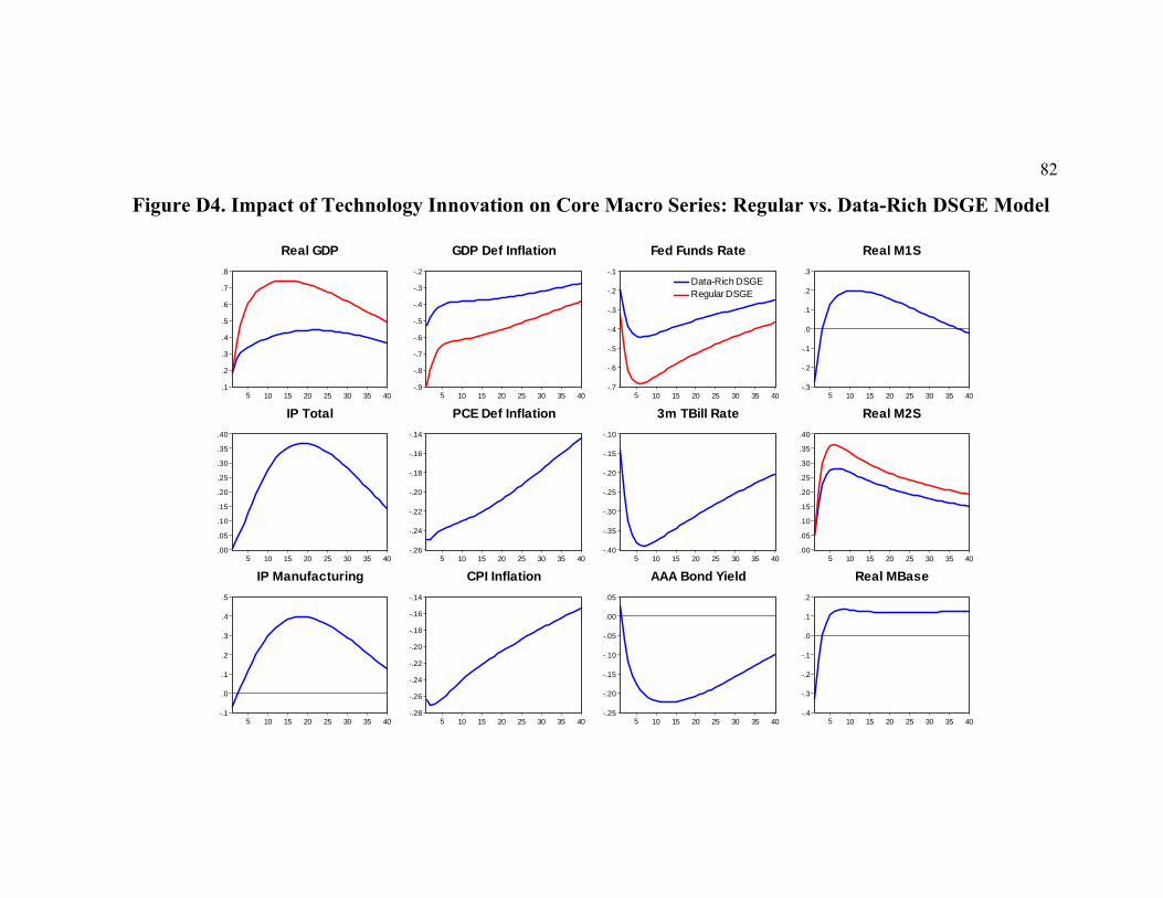
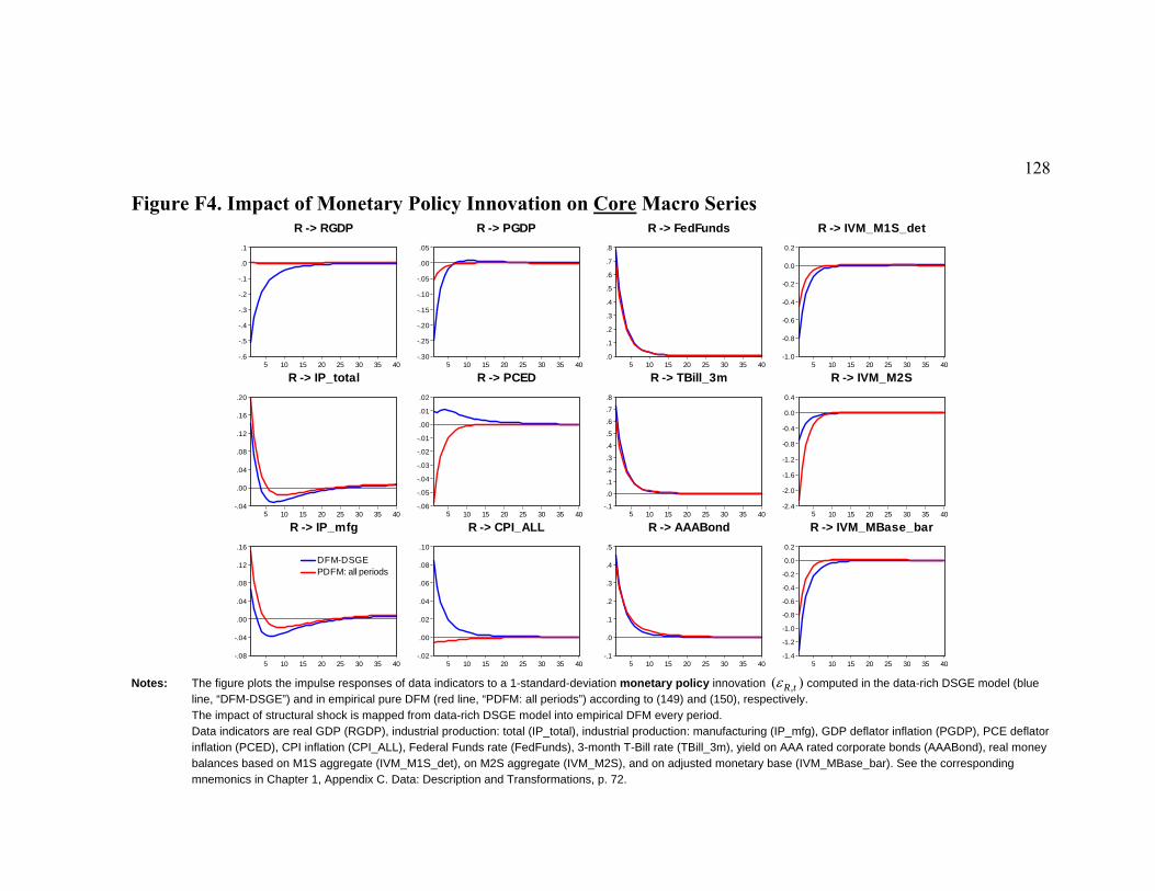
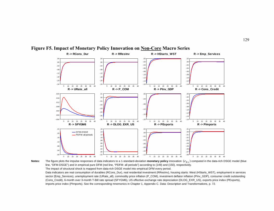
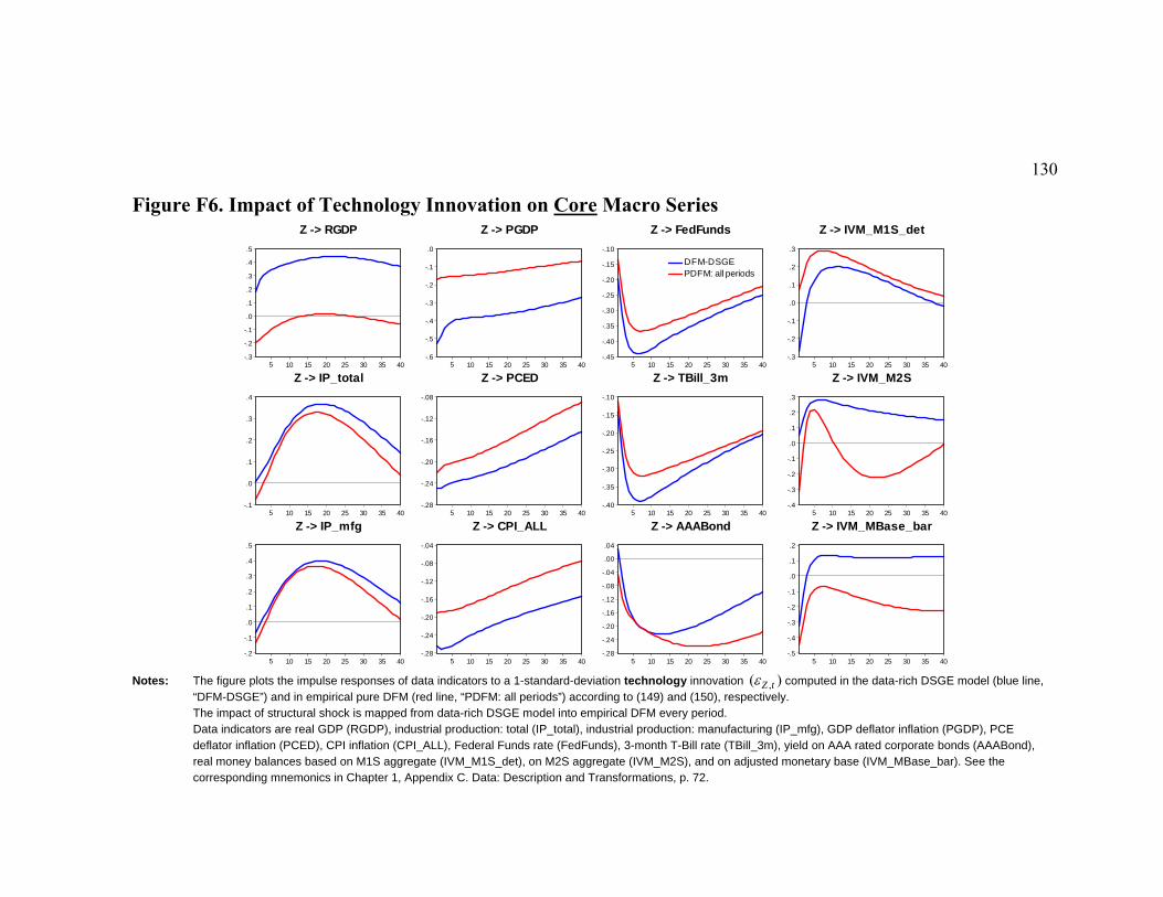
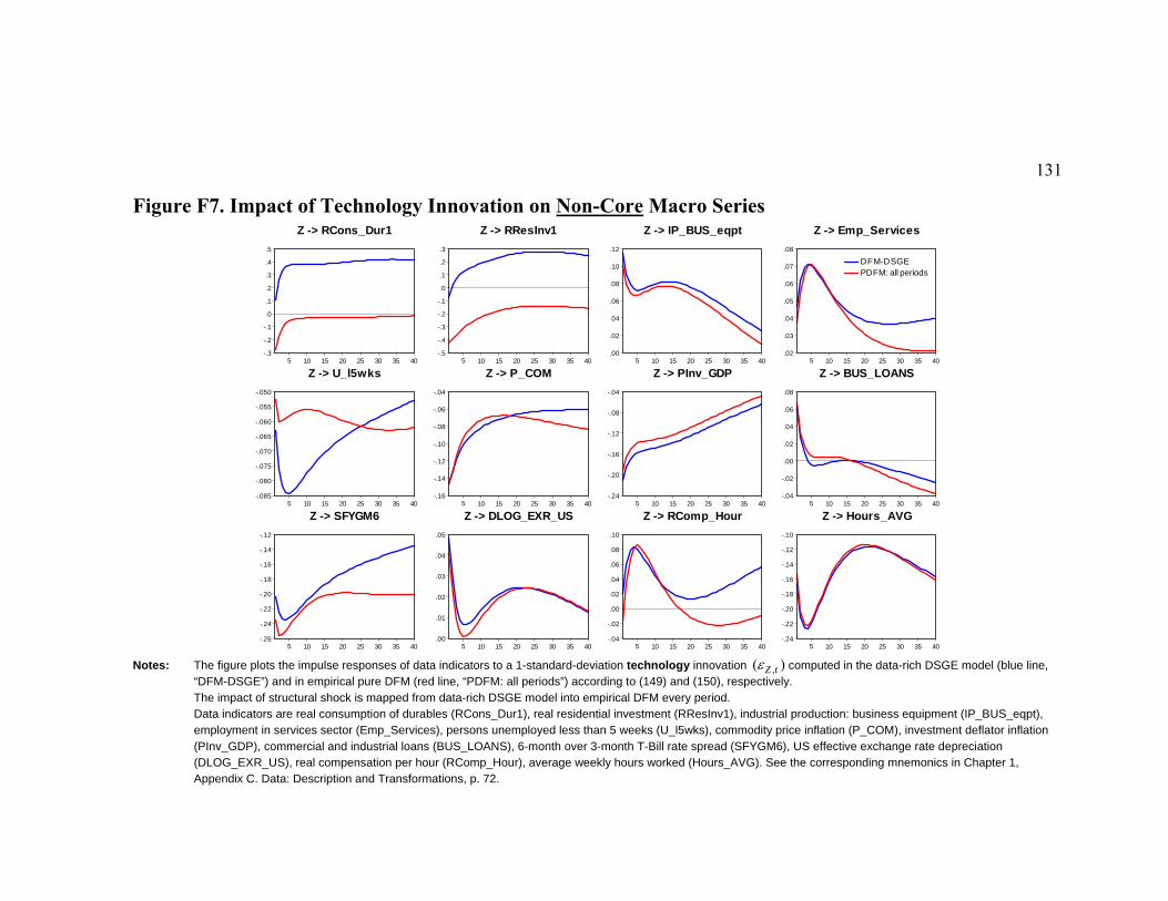
Chapter 2 “Data-Rich DSGE and Dynamic Factor Models”: In addition to a data-rich DSGE model with astandard New Keynesian core, we consider an unrestricted dynamic factor model and estimate both on a richpanel of U.S. macroeconomic and financial data compiled by Stock and Watson (2008). We find that thespaces spanned by the common empirical factors and by the data-rich DSGE model states are very close. First,this implies that a DSGE model indeed captures the essential sources of co-movement in the data and that thedifferences in fit between a data-rich DSGE model and a DFM are potentially due to restricted factor loadingsin the former. Second, this also implies a greater degree of comfort about propagation of structural shocks to awide array of macro and financial series. Third, the proximity of factor spaces facilitates economicinterpretation of a dynamic factor model, as the empirical factors are now isomorphic to the DSGE modelstate variables with clear economic meaning. Finally, the proximity of factor spaces allows us to propagatemonetary policy and technology innovations in an otherwise completely non-structural dynamic factor modelto obtain predictions for many more series than just a handful of traditional macro variables includingmeasures of real activity, price indices, labor market indicators, interest rate spreads, money and credit stocks,and exchange rates. We can therefore provide a more complete and comprehen-sive picture of the effects ofmonetary policy and technology shocks.
This dissertation is available at ScholarlyCommons: http://repository.upenn.edu/edissertations/139
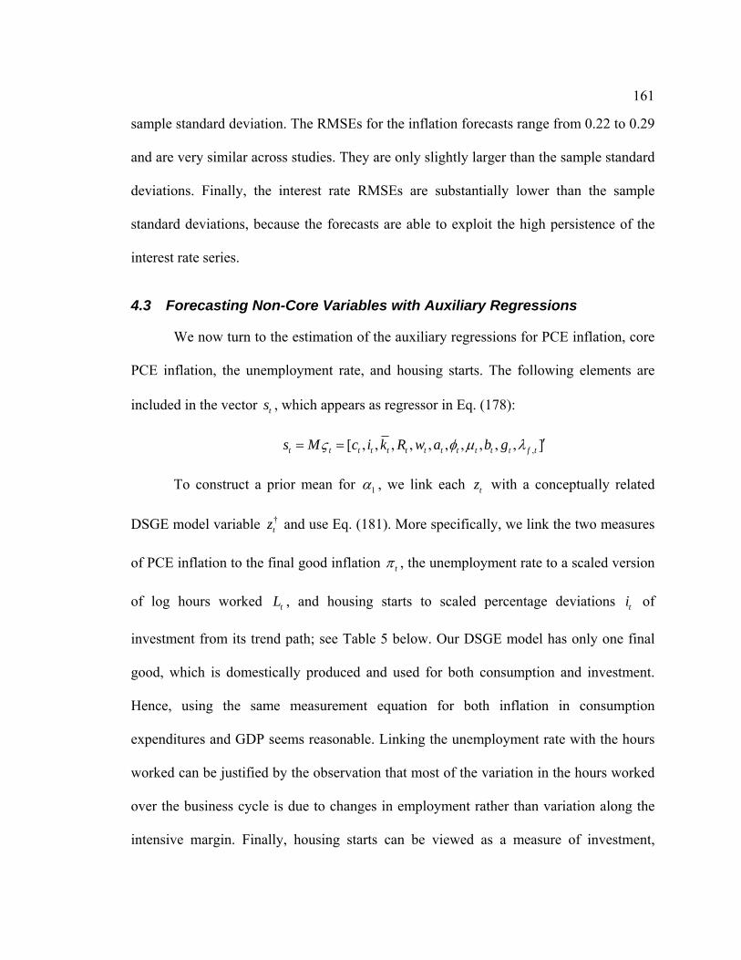
Chapter 3 “DSGE Model Based Forecasting of Non-Modeled Variables” (joint work with Frank Schorfheideand Keith Sill): We develop and illustrate a simple method to generate a DSGE model-based forecast forvariables that do not explicitly appear in the model (non-core variables). Estimation is performed in two steps.First, we estimate the regular DSGE model on core observables. Second, we obtain filtered DSGE model statevariables and use them as regressors in auxiliary linear regressions – resembling DFM measurement equations– for the non-core variables. Predictions for the non-core variables are then obtained by applying theirestimated measurement equations to DSGE model-generated forecasts of the state variables.
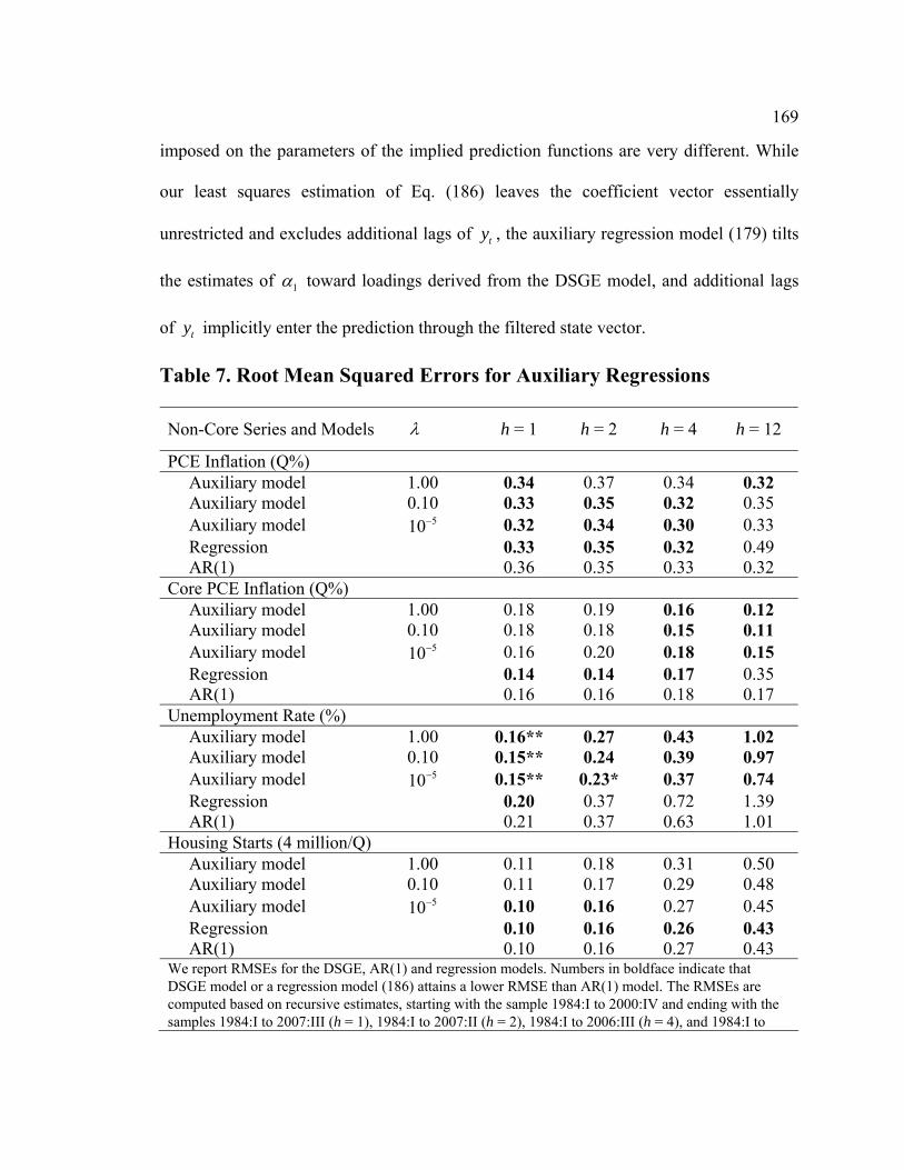
This estimation approach can be viewed as a simplified version of a data-rich DSGE model estimation inwhich we essentially decouple the analysis of the non-core measurement equations and the estimation of aDSGE model on the core observables. The proposed shortcut is practically appealing: we considerably reducethe associated computational costs and we can incorporate and forecast an additional non-core variablewithout having to re-estimate the whole DSGE model, a feature useful in real-time applications. We apply ourapproach to generate and evaluate recursive forecasts for personal consumption expenditure (PCE) inflation,core PCE inflation, the unemployment rate, and housing starts.
Acknowledgements The author is deeply grateful to his main advisor Frank Schorfheide, and the thesis committee members Frank Diebold and Jesús Fernández-Villaverde for the continued support, strong encouragement and wise guidance throughout the process of writing this dissertation. The author would also like to thank Cristina Fuentes-Albero, Yuriy Gorodnichenko, Ed Herbst, Dirk Krueger, Leonardo Melosi, Emanuel Moench, Andriy Norets, Keith Sill, Kevin Song, Sergiy Stetsenko and other participants of the Penn Econometrics Seminar, Penn Macro lunch and Penn Econometrics lunch for valuable discussions and many useful comments and suggestions.
iv
ABSTRACT
ESSAYS IN ESTIMATION OF DYNAMIC STOCHASTIC GENERAL EQUILIBRIUM MODELS
Maxym Kryshko
Frank Schorfheide
Dynamic factor models (DFM) and dynamic stochastic general equilibrium (DSGE) models are widely used for empirical research in macroeconomics. The empirical factor literature argues that the co-movement of large panels of macroeconomic and financial data can be captured by relatively few common unobserved factors. Similarly, the dynamics in DSGE models are often governed by a handful of state variables and exogenous processes such as latent preference and/or technology shocks. A general topic of this dissertation is the estimation of DSGE models on a rich panel of macroeconomic and financial data by combining a DSGE with a dynamic factor model. By incorporating richer information, this combination allows to obtain DSGE model predictions and to do more reliable policy analysis with a broader range of data series of interest than before. Moreover, the combination of a DSGE and a dynamic factor model can be used as a tool for evaluating a DSGE model. This dissertation consists of three essays summarized below.
Chapter 1 “Bayesian Dynamic Factor Analysis of a Simple Monetary DSGE Model”: We take a standard New Keynesian business cycle model to a richer data set. When estimating DSGE models, the number of observable economic variables is usually kept small, and for convenience it is assumed that the model variables are perfectly measured by a single – often quite arbitrarily selected – data series. We relax these two assumptions and estimate a fairly simple monetary DSGE model on a richer data set. Building upon Boivin and Giannoni (2006), the framework can be seen as a combination of a DSGE model and a dynamic factor model in which factors are economic state variables and the factor dynamics are governed by a DSGE model solution. Using post-1983 U.S. data on real output, inflation, nominal interest rates, measures of inverse money velocity, and a large panel of informational series, we compare the data-rich DSGE model with a regular – few observables, perfect measurement – DSGE model in terms of deep parameter estimates, propagation of monetary policy and technology shocks and sources of business cycle fluctuations. We document that the data-rich DSGE model generates a higher implied duration of Calvo price contracts and a lower slope of the New Keynesian Phillips curve. Because of the data set’s high panel dimension, the likelihood-based estimation of the data-rich DSGE model is computationally very
v
challenging. To reduce the costs, we employed a novel speedup as in Jungbacker and Koopman (2008) and achieved the computational time savings of 60 percent.
Chapter 2 “Data-Rich DSGE and Dynamic Factor Models”: In addition to a data-rich DSGE model with a standard New Keynesian core, we consider an unrestricted dynamic factor model and estimate both on a rich panel of U.S. macroeconomic and financial data compiled by Stock and Watson (2008). We find that the spaces spanned by the common empirical factors and by the data-rich DSGE model states are very close. First, this implies that a DSGE model indeed captures the essential sources of co-movement in the data and that the differences in fit between a data-rich DSGE model and a DFM are potentially due to restricted factor loadings in the former. Second, this also implies a greater degree of comfort about propagation of structural shocks to a wide array of macro and financial series. Third, the proximity of factor spaces facilitates economic interpretation of a dynamic factor model, as the empirical factors are now isomorphic to the DSGE model state variables with clear economic meaning. Finally, the proximity of factor spaces allows us to propagate monetary policy and technology innovations in an otherwise completely non-structural dynamic factor model to obtain predictions for many more series than just a handful of traditional macro variables including measures of real activity, price indices, labor market indicators, interest rate spreads, money and credit stocks, and exchange rates. We can therefore provide a more complete and comprehen-sive picture of the effects of monetary policy and technology shocks.
Chapter 3 “DSGE Model Based Forecasting of Non-Modeled Variables” (joint work with Frank Schorfheide and Keith Sill): We develop and illustrate a simple method to generate a DSGE model-based forecast for variables that do not explicitly appear in the model (non-core variables). Estimation is performed in two steps. First, we estimate the regular DSGE model on core observables. Second, we obtain filtered DSGE model state variables and use them as regressors in auxiliary linear regressions – resembling DFM measurement equations – for the non-core variables. Predictions for the non-core variables are then obtained by applying their estimated measurement equations to DSGE model-generated forecasts of the state variables.
This estimation approach can be viewed as a simplified version of a data-rich DSGE model estimation in which we essentially decouple the analysis of the non-core measurement equations and the estimation of a DSGE model on the core observables. The proposed shortcut is practically appealing: we considerably reduce the associated computational costs and we can incorporate and forecast an additional non-core variable without having to re-estimate the whole DSGE model, a feature useful in real-time applications. We apply our approach to generate and evaluate recursive forecasts for personal consumption expenditure (PCE) inflation, core PCE inflation, the unemployment rate, and housing starts.
vi
Table of Contents ACKNOWLEDGEMENTS....................................................................................................................... III LIST OF TABLES .................................................................................................................................. VIII LIST OF FIGURES ................................................................................................................................... IX CHAPTER 1. BAYESIAN DYNAMIC FACTOR ANALYSIS OF A SIMPLE MONETARY DSGE MODEL..........................................................................................................................................................1
2.1 Regular vs. Data-Rich DSGE Models .....................................................................................5 2.2 Environment ............................................................................................................................7
2.2.1 Households ........................................................................................................................................ 8 2.2.2 Final Good Firms............................................................................................................................. 11 2.2.3 Intermediate Goods Firms ............................................................................................................... 12 2.2.4 Monetary and Fiscal Policy ............................................................................................................. 16 2.2.5 Aggregation..................................................................................................................................... 17
3 ECONOMETRIC METHODOLOGY.......................................................................................................19 3.1 Estimation of the Data-Rich DSGE Model ............................................................................19 3.2 Speed-Up: Jungbacker and Koopman 2008 ..........................................................................26
4 DATA AND TRANSFORMATIONS .......................................................................................................29 5 EMPIRICAL RESULTS........................................................................................................................32
5.1 Priors.....................................................................................................................................32 5.2 Posteriors: Regular vs. Data-Rich DSGE Model ..................................................................37 5.3 Estimated States: Regular vs. Data-Rich DSGE Model ........................................................39 5.4 Sources of Business Cycle Fluctuations ................................................................................41 5.5 Impulse Response Analysis....................................................................................................44
6 CONCLUSIONS..................................................................................................................................49 APPENDIX A. DSGE MODEL .....................................................................................................................52
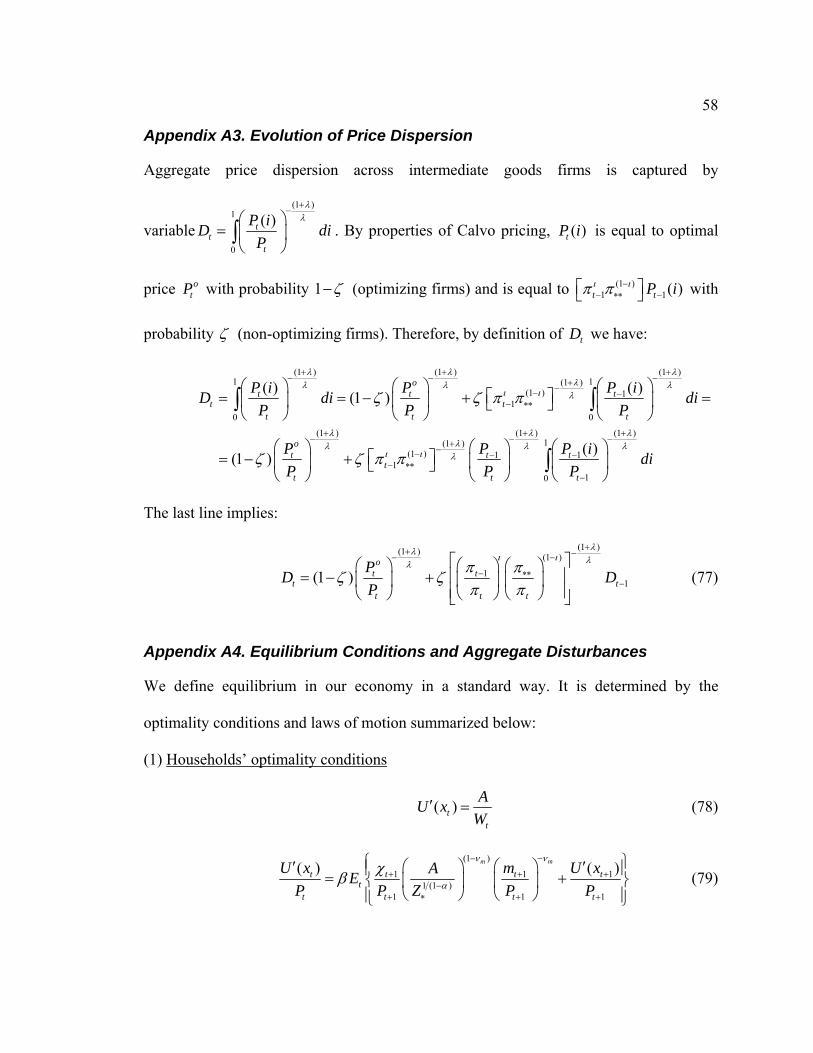
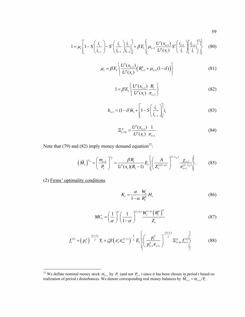
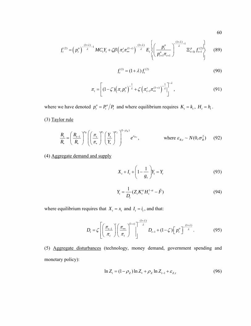
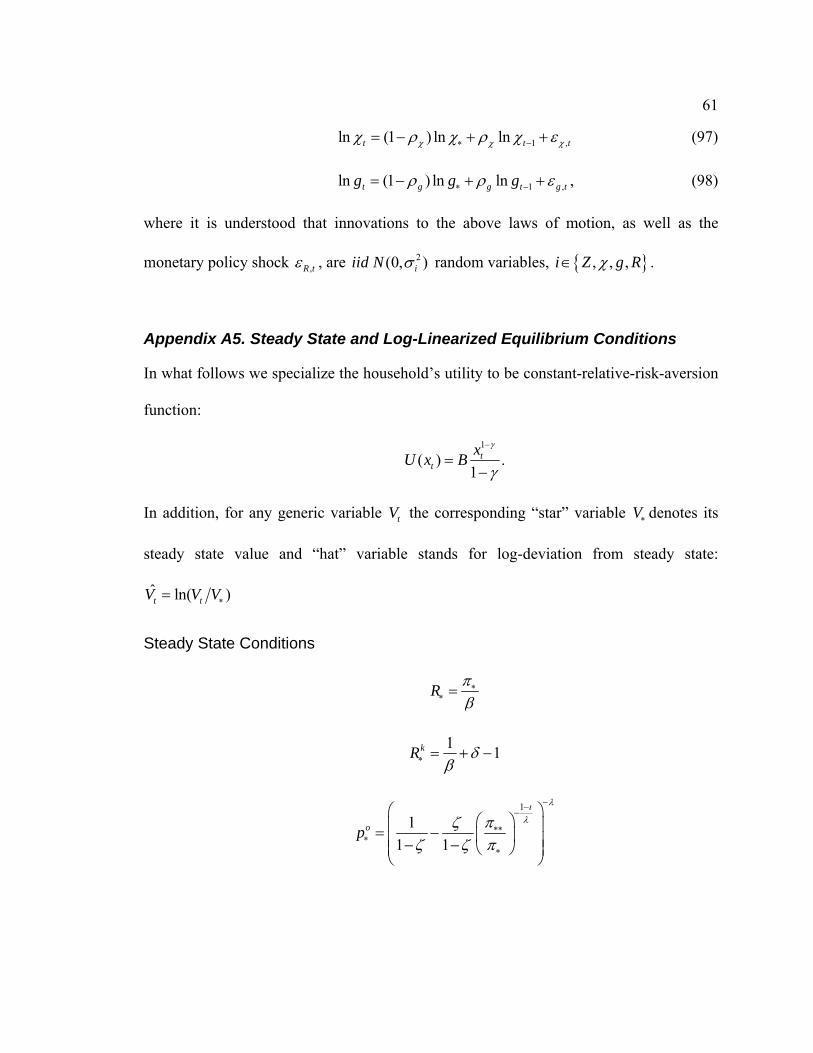
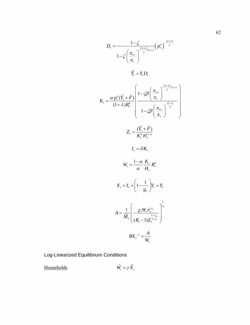
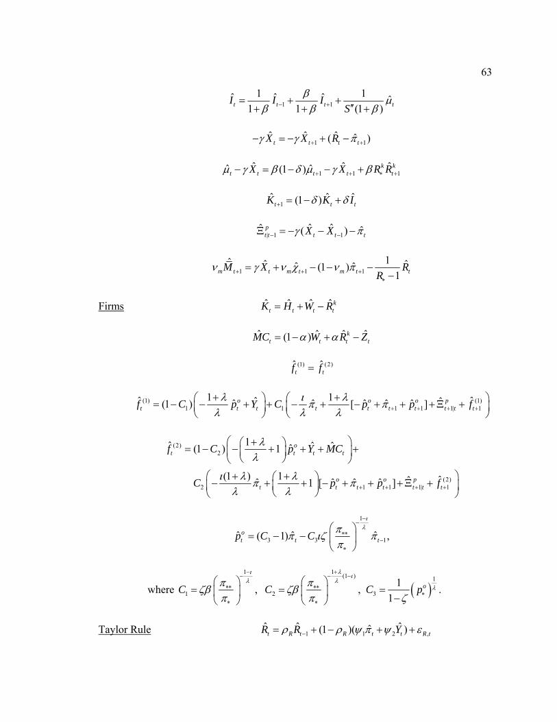
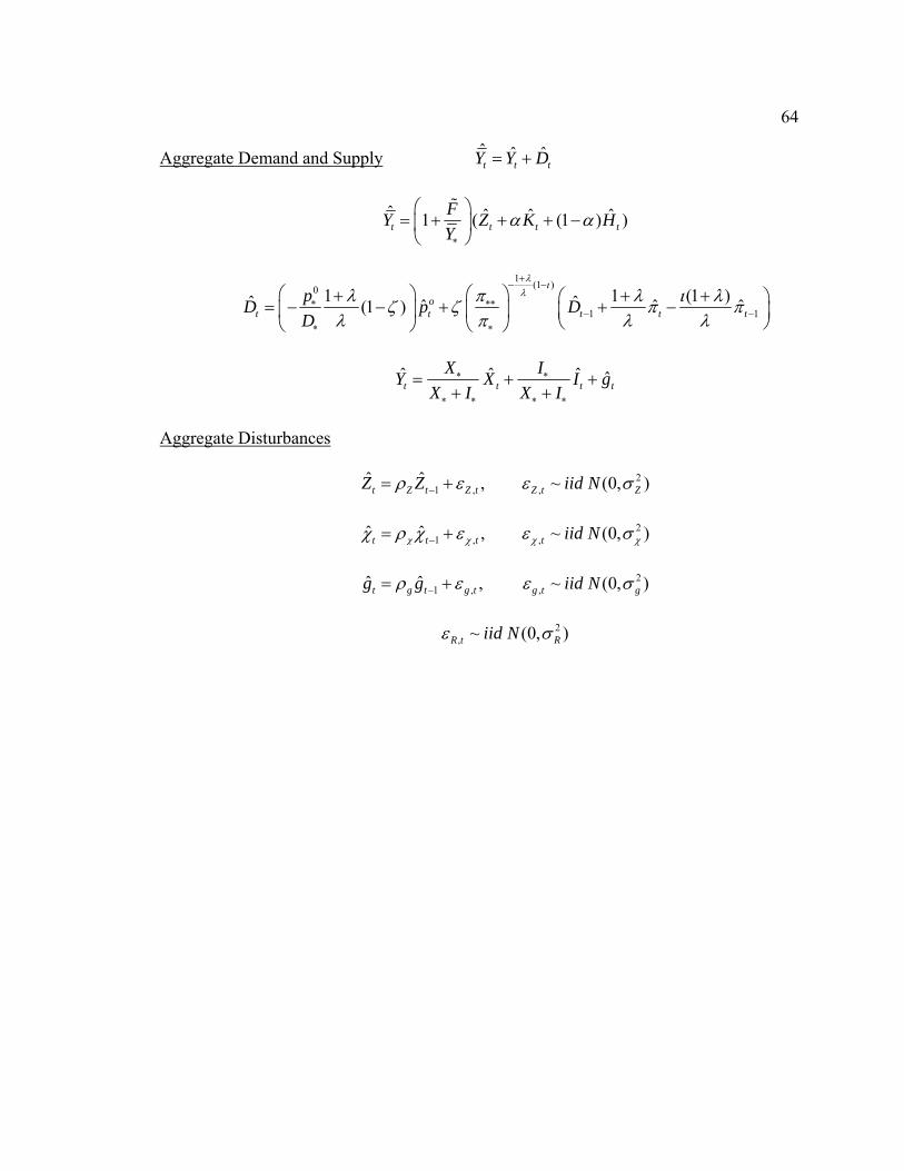
Appendix A1. First-Order Conditions of Household ...........................................................................52 Appendix A2. First-Order Conditions of Intermediate Goods Firm ....................................................54 Appendix A3. Evolution of Price Dispersion .......................................................................................58 Appendix A4. Equilibrium Conditions and Aggregate Disturbances...................................................58 Appendix A5. Steady State and Log-Linearized Equilibrium Conditions ............................................61
APPENDIX B. DETAILS OF MARKOV CHAIN MONTE CARLO ALGORITHM .................................................65 APPENDIX C. DATA: DESCRIPTION AND TRANSFORMATIONS....................................................................72 APPENDIX D. TABLES AND FIGURES..........................................................................................................74
CHAPTER 2. DATA-RICH DSGE AND DYNAMIC FACTOR MODELS .........................................83 1 INTRODUCTION ................................................................................................................................83 2 TWO MODELS ..................................................................................................................................88
2.1 Dynamic Factor Model..........................................................................................................88 2.2 Data-Rich DSGE Model ........................................................................................................89
3 ECONOMETRIC METHODOLOGY.......................................................................................................91 3.1 Estimation of the Data-Rich DSGE Model ............................................................................91 3.2 Estimation of the Dynamic Factor Model..............................................................................91
4 DATA ...............................................................................................................................................98 5 EMPIRICAL ANALYSIS......................................................................................................................99
5.1 Priors and Posteriors ..........................................................................................................100
vii
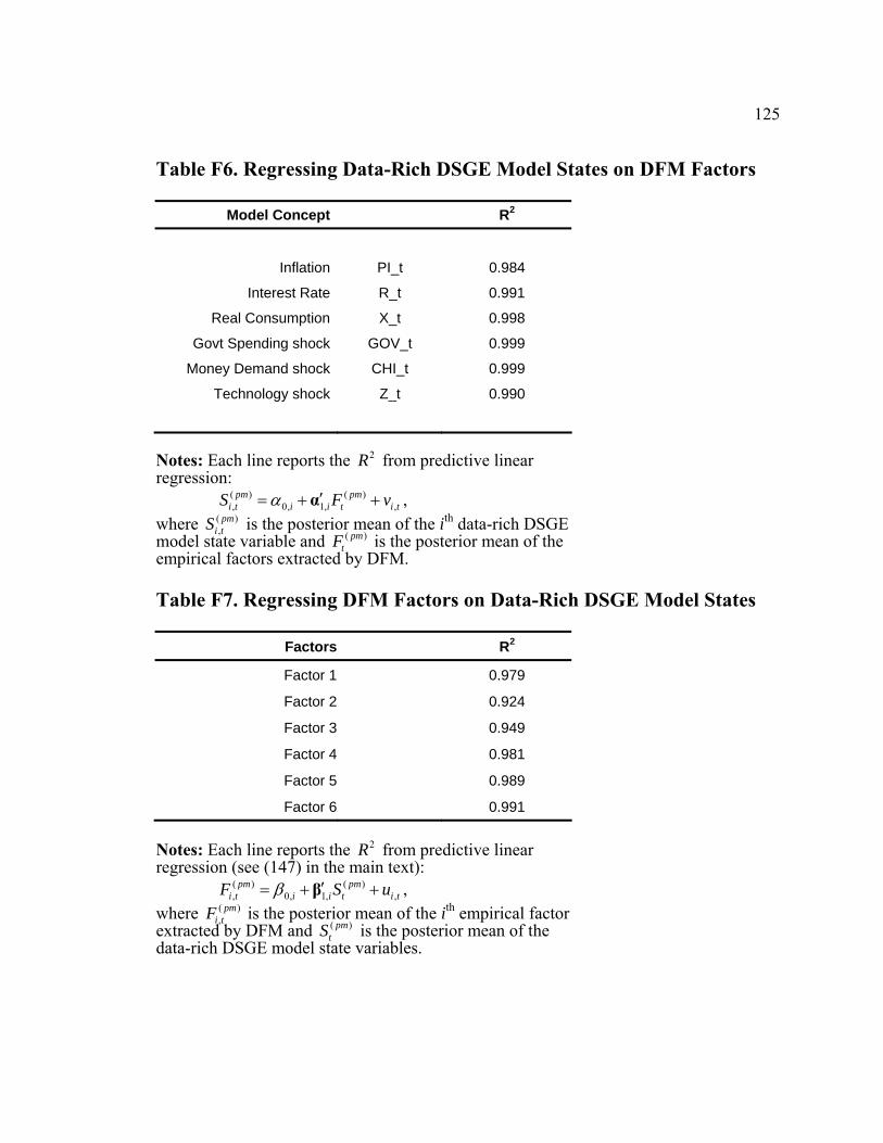
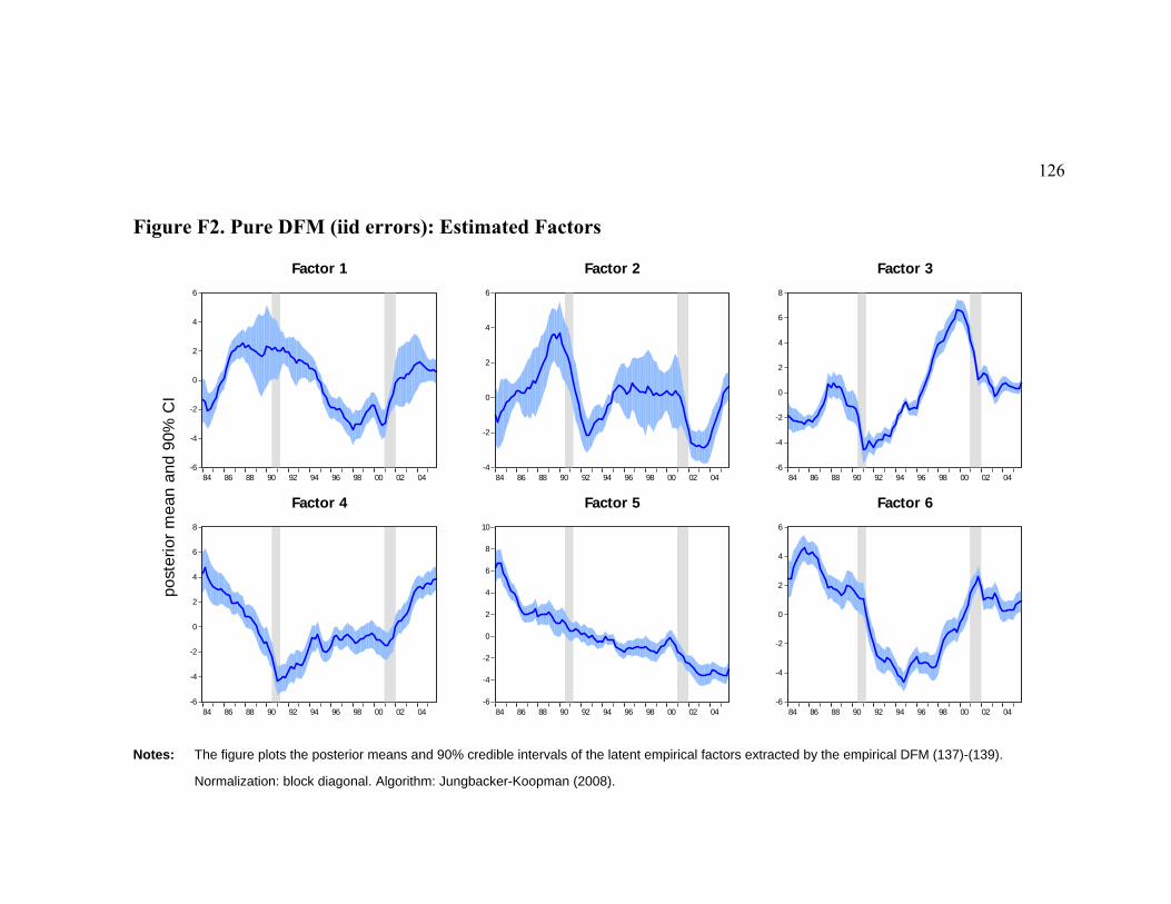
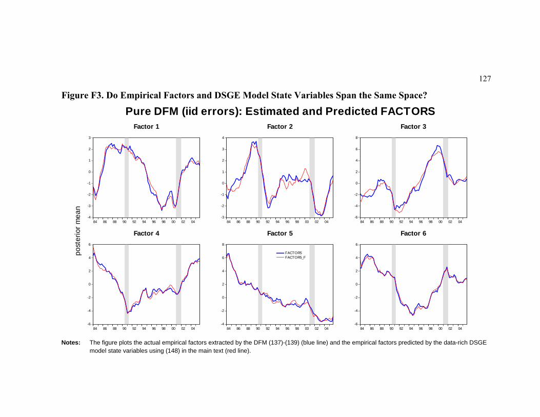
5.2 Empirical Factors and Estimated DSGE Model States .......................................................102 5.3 How Well Factors Trace Data.............................................................................................103 5.4 Comparing Factor Spaces ...................................................................................................105 5.5 Propagation of Monetary Policy and Technology Innovations ...........................................106
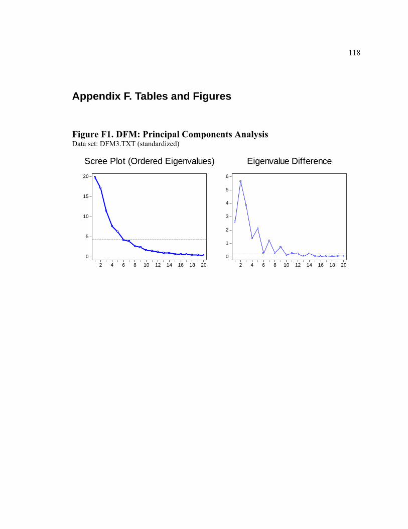
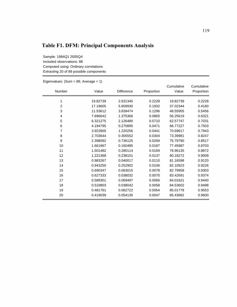
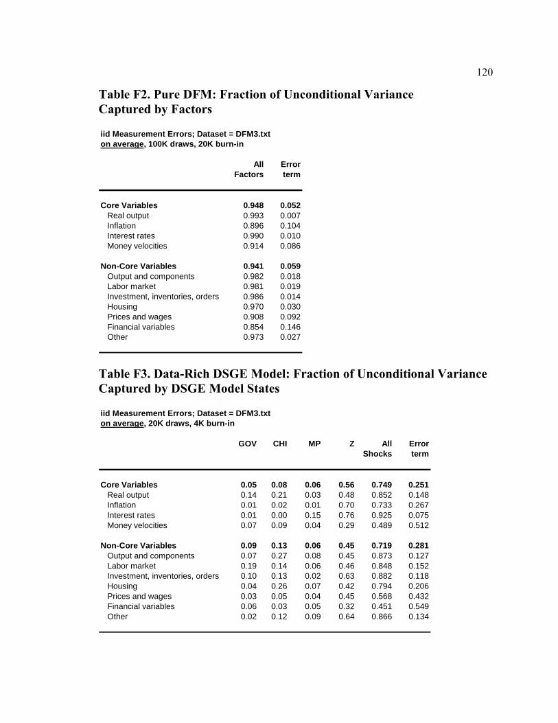
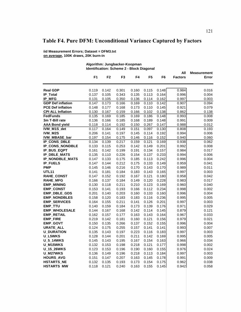
6 CONCLUSIONS................................................................................................................................115 APPENDIX E. DFM: GIBBS SAMPLER: DRAWING TRANSITION EQUATION MATRIX ................................116 APPENDIX F. TABLES AND FIGURES ........................................................................................................118
CHAPTER 3. DSGE MODEL BASED FORECASTING OF NON-MODELED VARIABLES.......132 1 INTRODUCTION ..............................................................................................................................132 2 THE DSGE MODEL........................................................................................................................136 3 ECONOMETRIC METHODOLOGY.....................................................................................................142
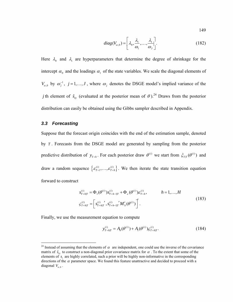
3.1 DSGE Model Estimation .....................................................................................................143 3.2 Linking Model States to Non-Core Variables......................................................................145 3.3 Forecasting..........................................................................................................................149
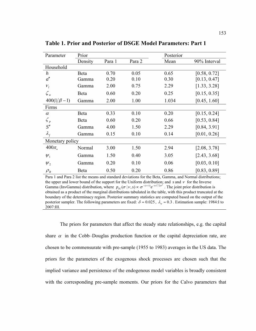
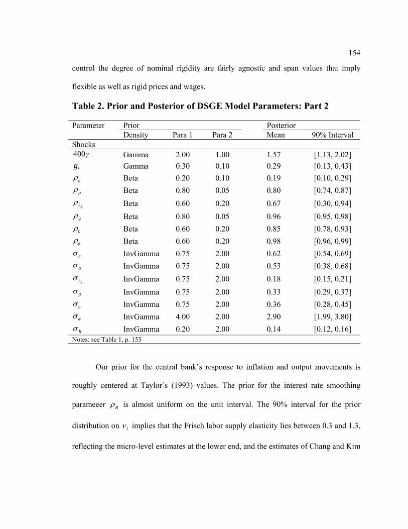
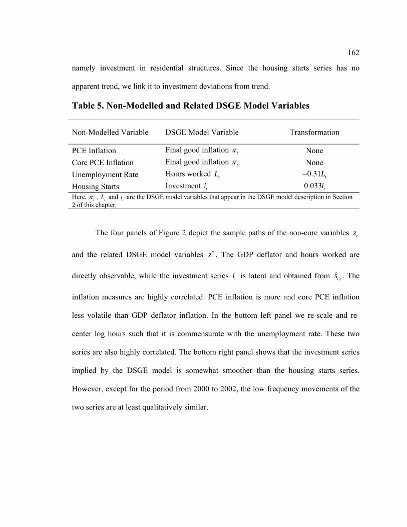
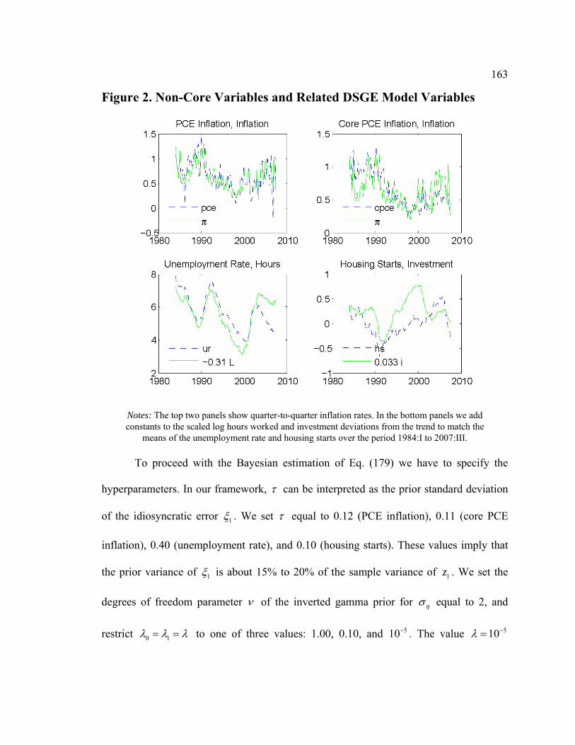
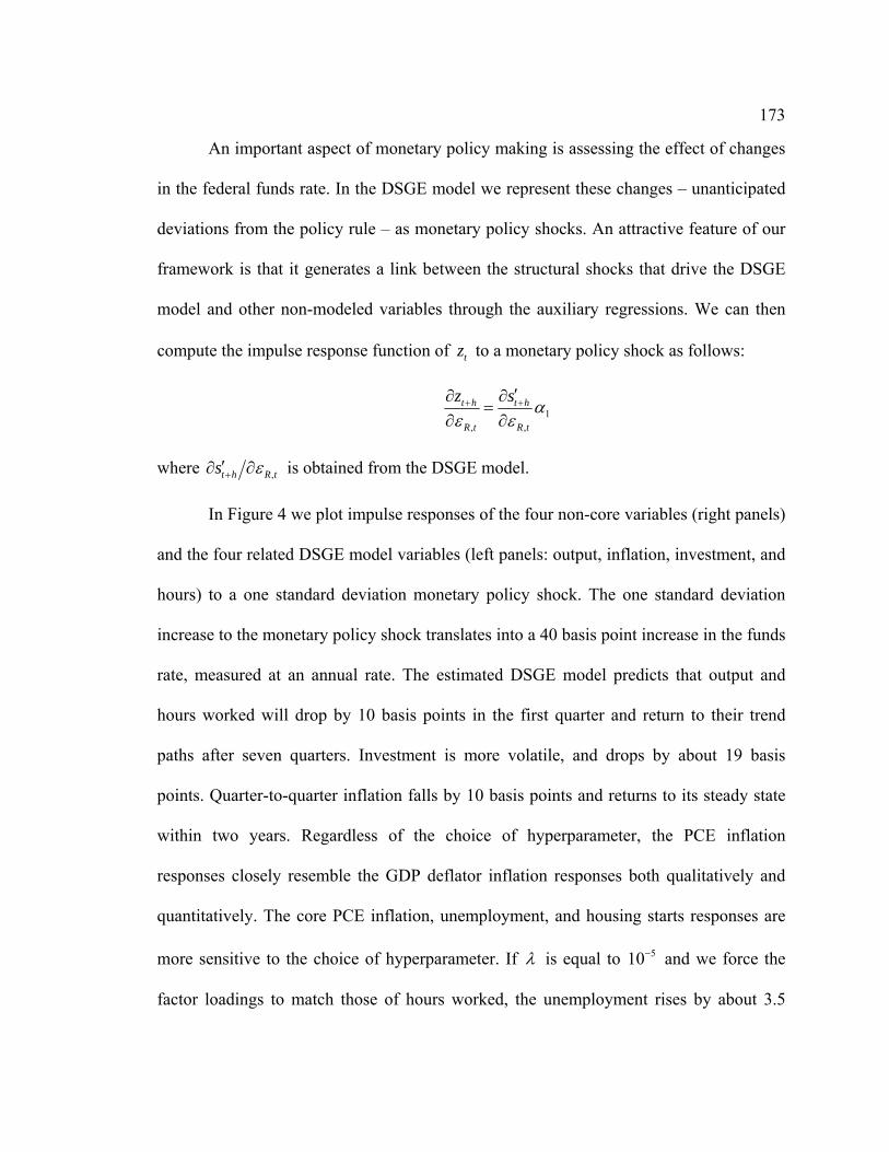
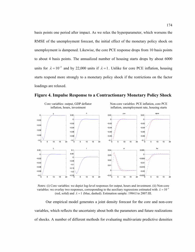
4 EMPIRICAL APPLICATION...............................................................................................................150 4.1 Data and Priors...................................................................................................................151 4.2 DSGE Model Estimaton and Forecasting of Core Variables ..............................................155 4.3 Forecasting Non-Core Variables with Auxiliary Regressions.............................................161 4.4 Multivariate Considerations................................................................................................171
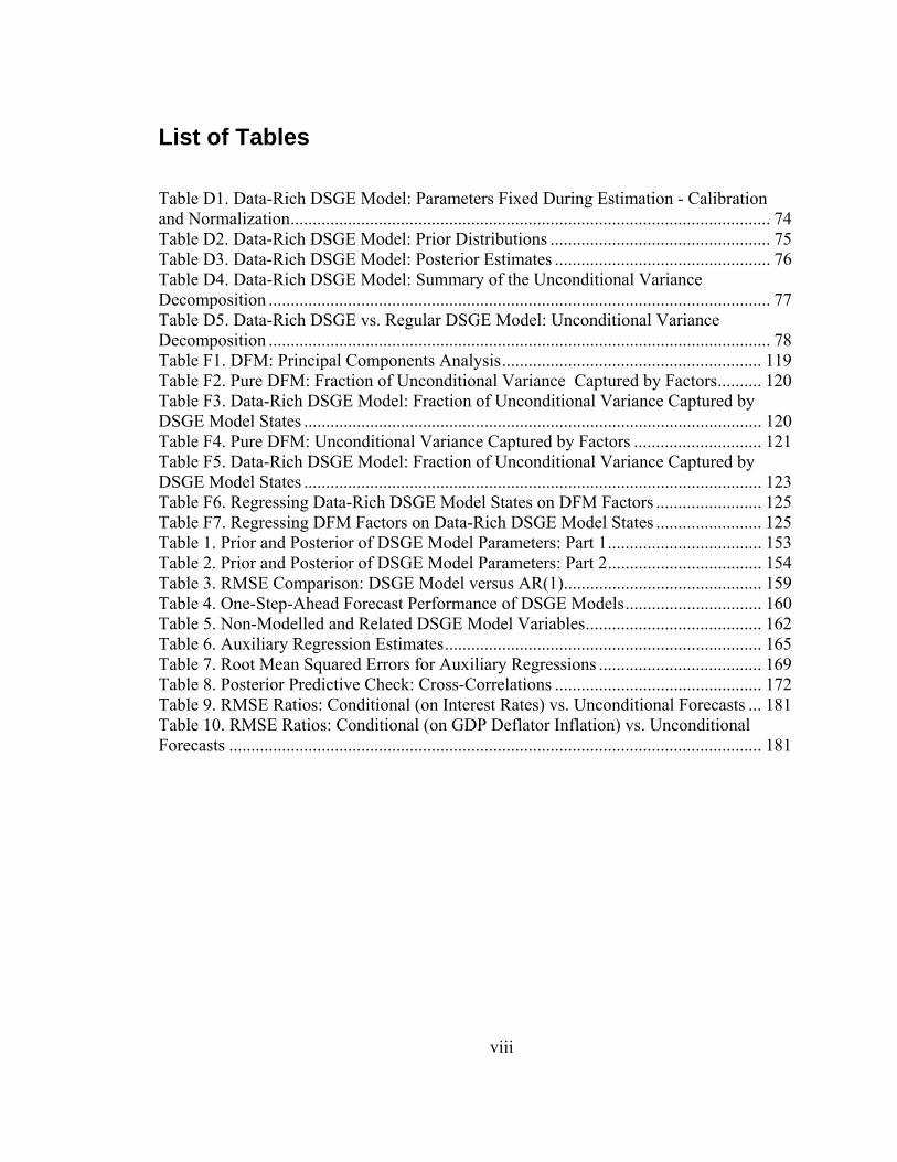
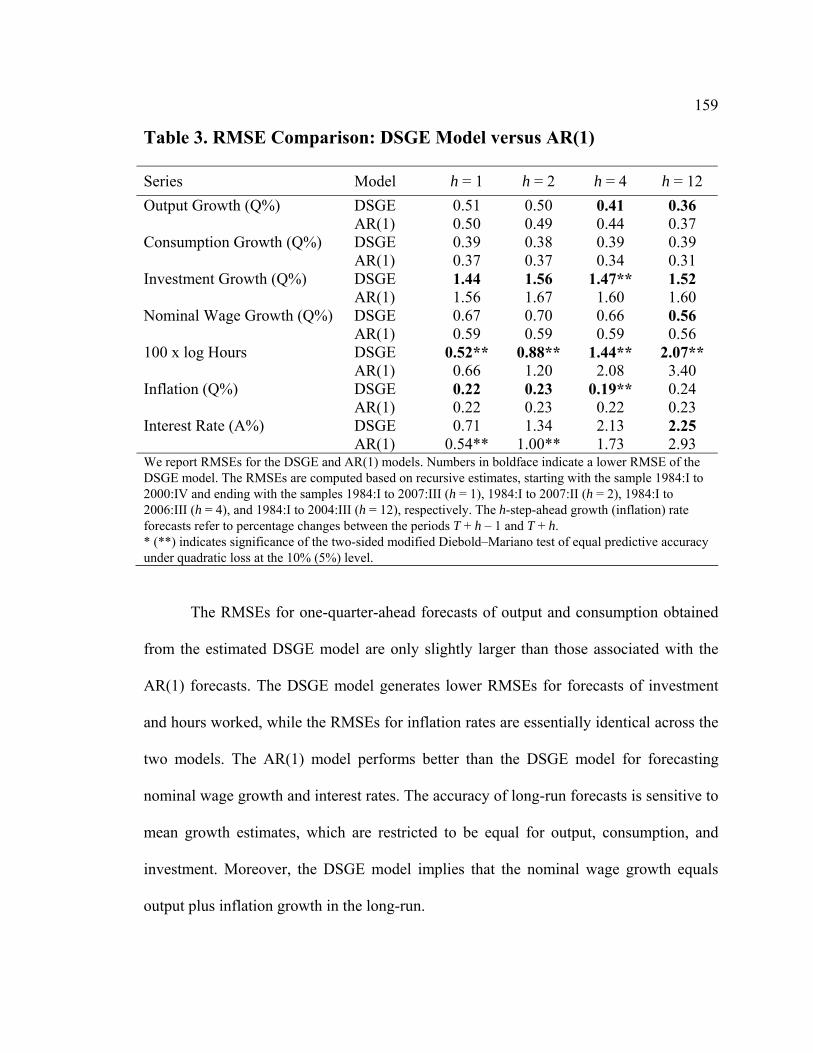
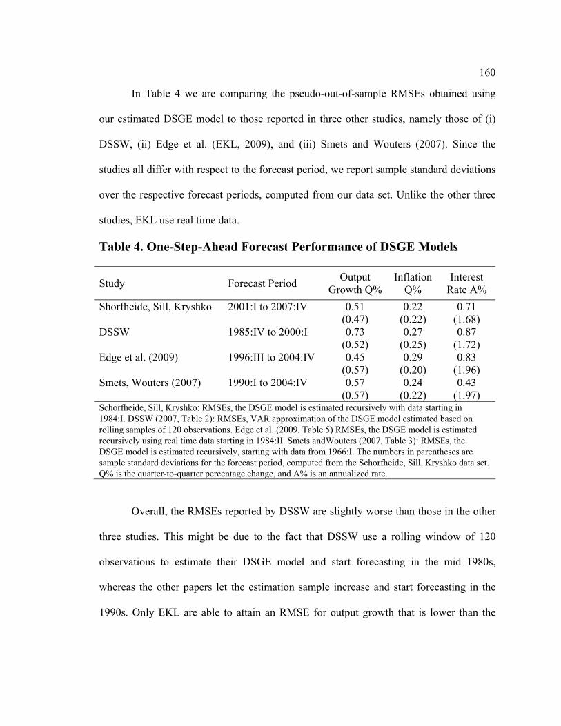
List of Tables Table D1. Data-Rich DSGE Model: Parameters Fixed During Estimation - Calibration and Normalization............................................................................................................. 74 Table D2. Data-Rich DSGE Model: Prior Distributions .................................................. 75 Table D3. Data-Rich DSGE Model: Posterior Estimates ................................................. 76 Table D4. Data-Rich DSGE Model: Summary of the Unconditional Variance Decomposition .................................................................................................................. 77 Table D5. Data-Rich DSGE vs. Regular DSGE Model: Unconditional Variance Decomposition .................................................................................................................. 78 Table F1. DFM: Principal Components Analysis........................................................... 119 Table F2. Pure DFM: Fraction of Unconditional Variance Captured by Factors.......... 120 Table F3. Data-Rich DSGE Model: Fraction of Unconditional Variance Captured by DSGE Model States ........................................................................................................ 120 Table F4. Pure DFM: Unconditional Variance Captured by Factors ............................. 121 Table F5. Data-Rich DSGE Model: Fraction of Unconditional Variance Captured by DSGE Model States ........................................................................................................ 123 Table F6. Regressing Data-Rich DSGE Model States on DFM Factors ........................ 125 Table F7. Regressing DFM Factors on Data-Rich DSGE Model States ........................ 125 Table 1. Prior and Posterior of DSGE Model Parameters: Part 1................................... 153 Table 2. Prior and Posterior of DSGE Model Parameters: Part 2................................... 154 Table 3. RMSE Comparison: DSGE Model versus AR(1)............................................. 159 Table 4. One-Step-Ahead Forecast Performance of DSGE Models............................... 160 Table 5. Non-Modelled and Related DSGE Model Variables........................................ 162 Table 6. Auxiliary Regression Estimates........................................................................ 165 Table 7. Root Mean Squared Errors for Auxiliary Regressions ..................................... 169 Table 8. Posterior Predictive Check: Cross-Correlations ............................................... 172 Table 9. RMSE Ratios: Conditional (on Interest Rates) vs. Unconditional Forecasts ... 181 Table 10. RMSE Ratios: Conditional (on GDP Deflator Inflation) vs. Unconditional Forecasts ......................................................................................................................... 181
ix
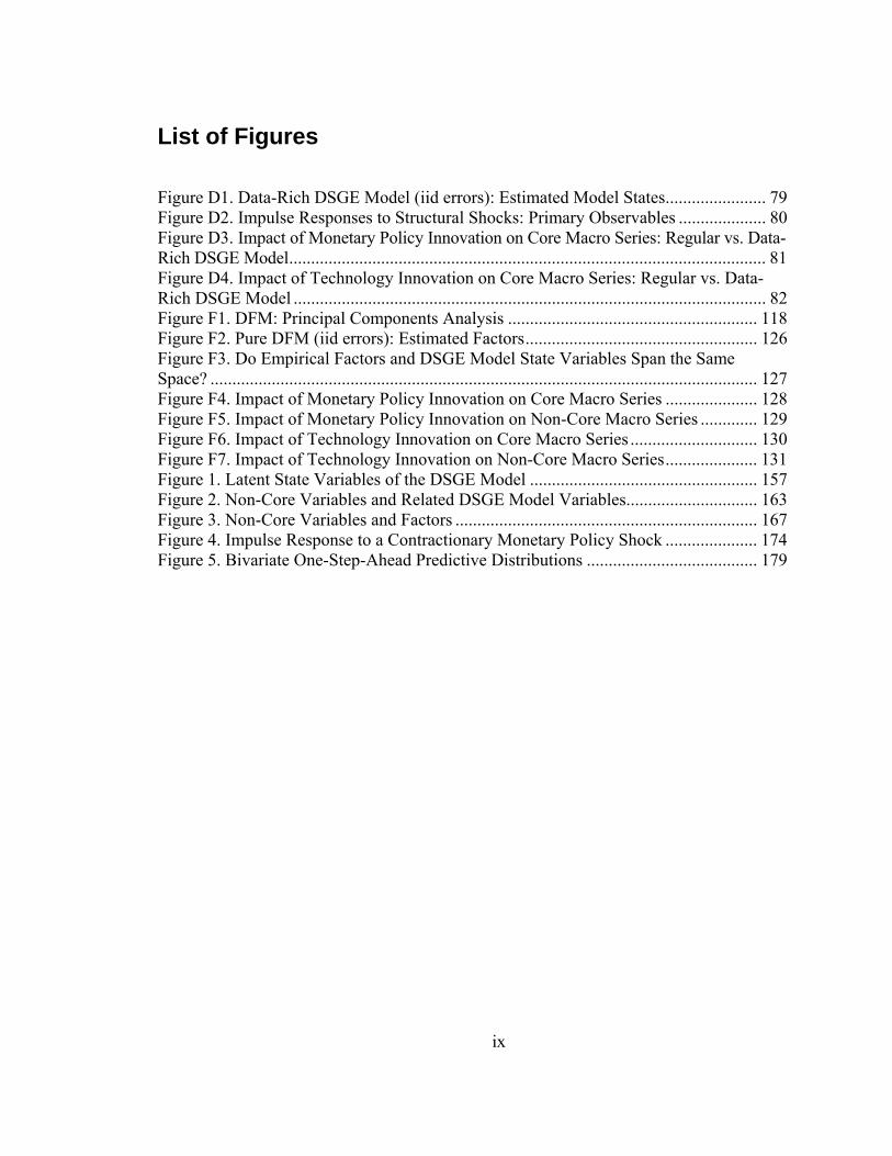
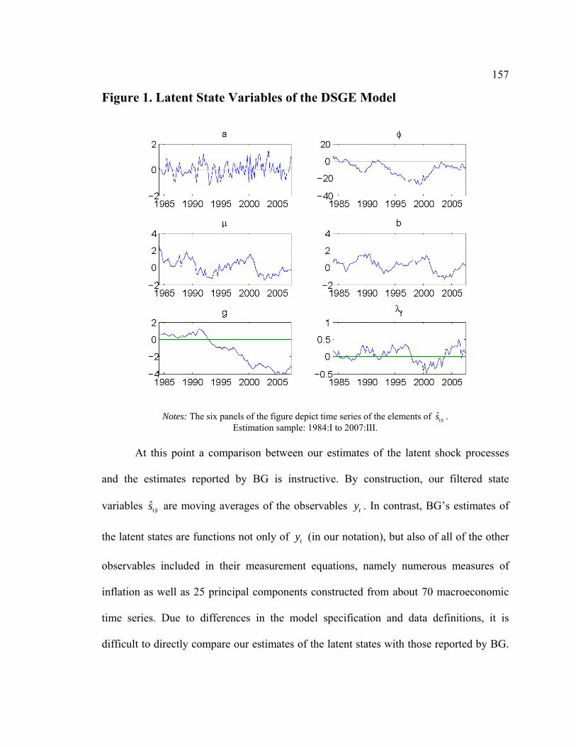
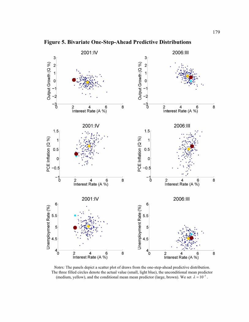
List of Figures Figure D1. Data-Rich DSGE Model (iid errors): Estimated Model States....................... 79 Figure D2. Impulse Responses to Structural Shocks: Primary Observables .................... 80 Figure D3. Impact of Monetary Policy Innovation on Core Macro Series: Regular vs. Data-Rich DSGE Model............................................................................................................. 81 Figure D4. Impact of Technology Innovation on Core Macro Series: Regular vs. Data-Rich DSGE Model ............................................................................................................ 82 Figure F1. DFM: Principal Components Analysis ......................................................... 118 Figure F2. Pure DFM (iid errors): Estimated Factors..................................................... 126 Figure F3. Do Empirical Factors and DSGE Model State Variables Span the Same Space? ............................................................................................................................. 127 Figure F4. Impact of Monetary Policy Innovation on Core Macro Series ..................... 128 Figure F5. Impact of Monetary Policy Innovation on Non-Core Macro Series ............. 129 Figure F6. Impact of Technology Innovation on Core Macro Series ............................. 130 Figure F7. Impact of Technology Innovation on Non-Core Macro Series..................... 131 Figure 1. Latent State Variables of the DSGE Model .................................................... 157 Figure 2. Non-Core Variables and Related DSGE Model Variables.............................. 163 Figure 3. Non-Core Variables and Factors ..................................................................... 167 Figure 4. Impulse Response to a Contractionary Monetary Policy Shock ..................... 174 Figure 5. Bivariate One-Step-Ahead Predictive Distributions ....................................... 179
1
CHAPTER 1. BAYESIAN DYNAMIC FACTOR ANALYSIS OF A SIMPLE MONETARY DSGE MODEL
1 Introduction When estimating dynamic stochastic general equilibrium (DSGE) models, the number of
observable economic variables is usually kept small, and for convenience it is assumed
that the model variables are perfectly measured by a single – often quite arbitrarily
selected – data series. In this chapter, we relax these two assumptions and estimate a
version of the monetary DSGE model with a standard New Keynesian core on a richer
data set. Building upon Boivin and Giannoni (2006), this so called data-rich DSGE
model can be seen as a combination of a regular DSGE model and a dynamic factor
model in which factors are the economic state variables of the DSGE model and the
transition of factors is governed by a DSGE model solution.
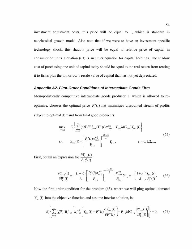
We use the post-1983 U.S. data on real output, inflation, nominal interest rates,
measures of inverse money velocity and a large panel of the other informational
macroeconomic and financial series compiled by Stock and Watson (2008) to estimate
and compare the new data-rich DSGE model with a regular – few observables, perfect
measurement – DSGE model, both sharing the same theoretical core. The estimation
2
involves Bayesian Markov Chain Monte Carlo (MCMC) methods. Because of the data
set’s high panel dimension, the likelihood-based estimation of the data-rich DSGE model
is computationally very challenging. To reduce the costs, we employed a novel speed-up
as in Jungbacker and Koopman (2008) and achieved the computational time savings of
60 percent.
We document that the data-rich DSGE model generates a higher duration of the
Calvo price contracts and a lower implied slope of the New Keynesian Phillips curve
measuring the elasticity of current inflation to real marginal costs. As we move from the
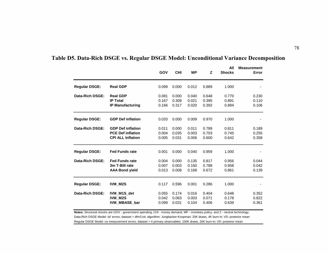
regular to the data-rich DSGE model, we find that: (i) the role of technology innovations
in generating fluctuations in real output, inflation and the interest rates is noticeably
reduced; and that (ii) the contribution of monetary policy shocks to cyclical fluctuations
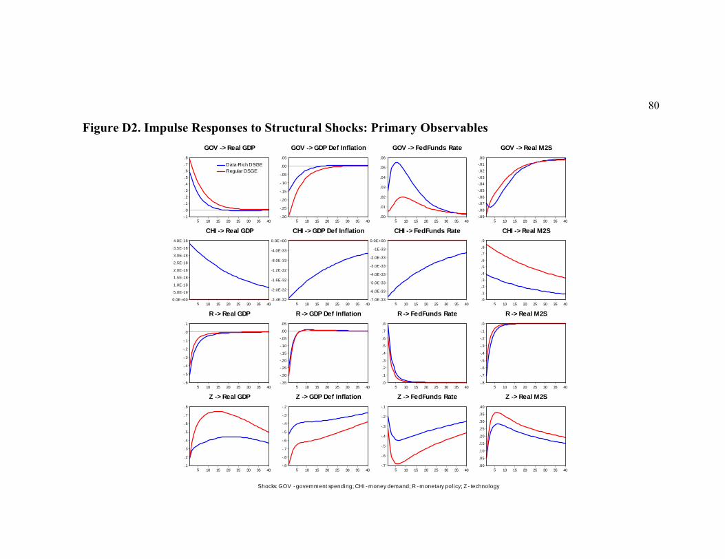
of the interest rates increases from 4 to 14-17 percent. Regarding dynamic propagation,
we establish that (i) despite some slight on-impact differences, the responses of all
primary observables (real GDP, GDP deflator inflation, fed funds rate and real M2) to the
monetary policy innovation remain theoretically plausible and quantitatively close in the
regular and in the data-rich DSGE models; and that (ii) the regular DSGE model tends to
overestimate all effects of TFP shocks, though on impact they might not have been too
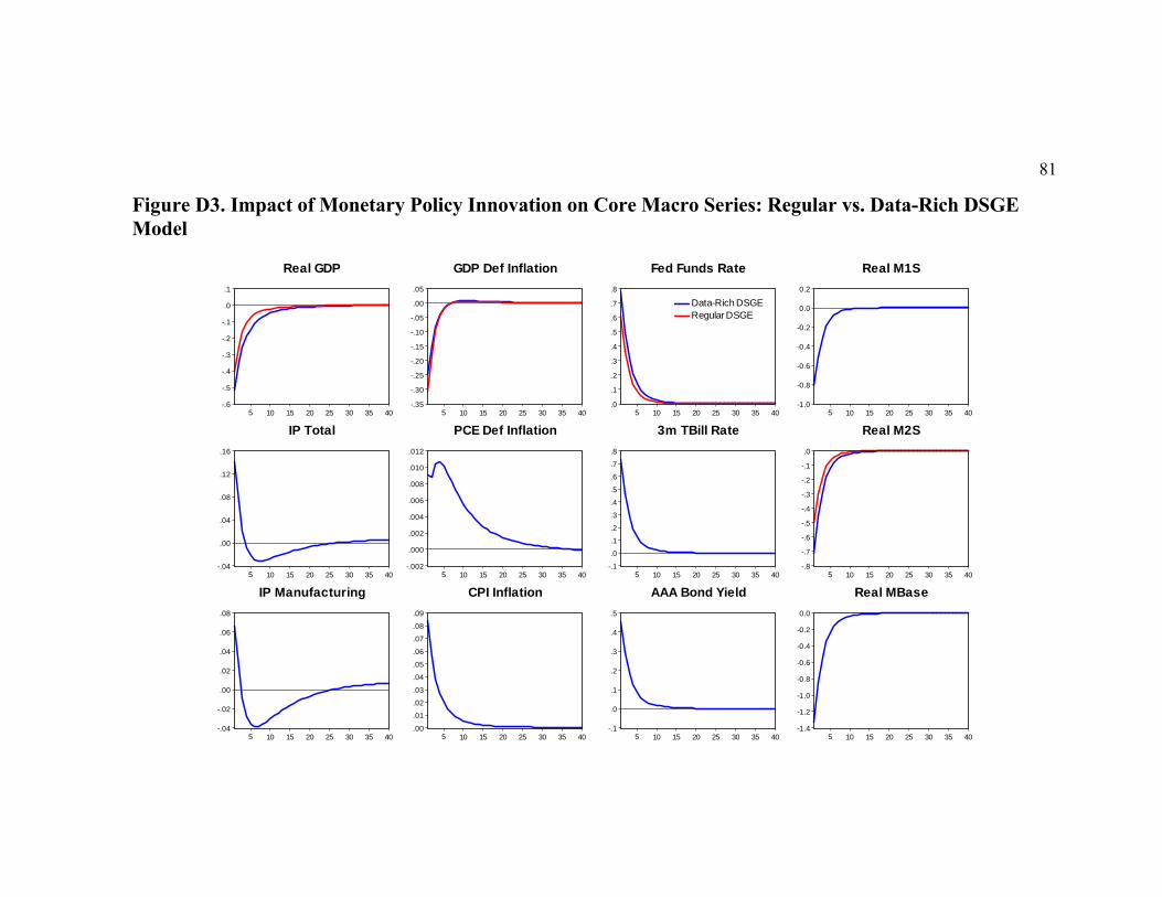
different. Finally, we find some puzzling results for the responses of the industrial
production, the PCE deflator inflation and the CPI inflation to monetary tightening,
which may indicate the potential misspecification of our theoretical DSGE model.
The chapter is organized as follows. In Section 2, we present a data-rich DSGE
model with a New Keynesian core to be used in the subsequent empirical analysis. Our
3
econometric methodology to estimate the data-rich DSGE model and also the
Jungbacker-Koopman computational speed-up are discussed in Section 3. Section 4
describes our data set and transformations. In Section 5 we proceed by conducting the
empirical analysis of the regular and the data-rich DSGE models. We begin by discussing
the choice of the prior distributions of model parameters and then describe the posterior
estimates of deep structural parameters in both models. Second, we compare the
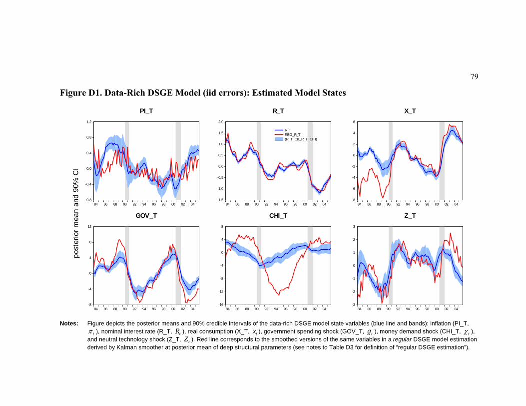
estimated DSGE state variables from our data-rich and from the regular DSGE model.
Finally, we explore the differences that the regular and the data-rich DSGE models imply
about the sources of business cycle fluctuations and about the propagation of structural
innovations, notably the monetary policy and technology shocks, to the real output,
inflation, interest rates and the real money balances. Section 6 concludes.
2 Data-Rich DSGE Model In this section, we begin by defining what we refer to as the data-rich DSGE model and
contrast it with the regular DSGE model. Then, we present a fairly standard New
Keynesian business cycle core that will be shared by both types of models.
In any DSGE model, economic agents solve intertemporal optimization problems
built from explicit preferences and technology assumptions. Moreover, decision rules of
these agents depend upon a number of exogenous stochastic disturbances that
characterize uncertainty in the economic environment. The equilibrium dynamics of a
DSGE model are captured by a system of non-linear expectational difference equations.
The standard approach in the literature is to derive a log-linear approximation to this non-
4
linear system around its deterministic steady state and then to solve numerically the
resulting linear rational expectations system by one of the available methods.1
This numerical solution delivers a vector autoregressive process for tS , the vector
collecting all non-redundant state variables of the DSGE model, and a linear relationship
between the remaining DSGE model variables tz and the current state tS :
( )t tz S= D θ (1)
1 , where ~ (0, ).t t t tS S iid Nε ε−= +G(θ) H(θ) Q(θ) (2)
The matrices in (1) and (2) are the functions of structural parameters θ characterizing
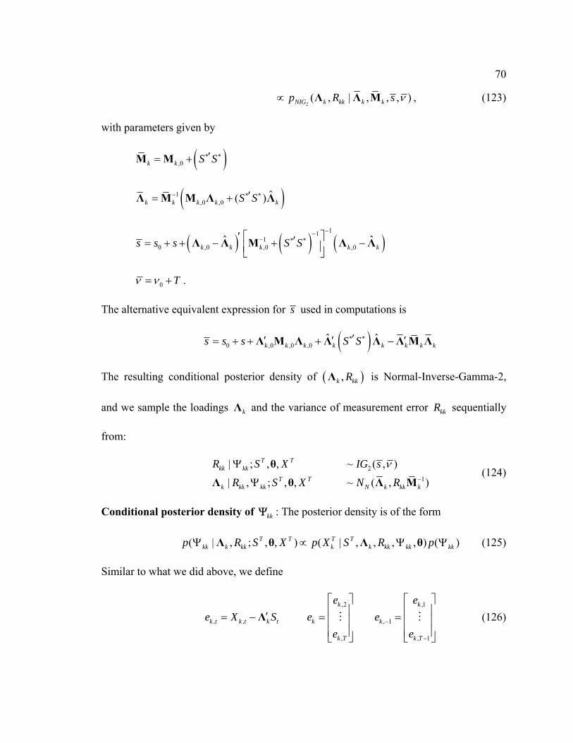
preferences and technology in a DSGE model. For convenience, we assume that the
exogenous shocks tε are mean-zero normal random variables with diagonal covariance
matrix Q(θ) . In what follows we will refer to tS as the DSGE model states or the DSGE
model state variables. We will also refer to the elements of [ , ]t t tS z S′ ′ ′= , the vector
collecting all variables in a given DSGE model, as the DSGE model concepts or simply
model concepts. The typical examples of model concepts could be inflation, output,
technology shock, capital stock and so on. By definition of tS :
( )
t tS S⎡ ⎤
= ⎢ ⎥⎣ ⎦
D θI
(3)
In order to estimate our DSGE model on a set of observables 1[ ,..., ]TTX X X ′= , a
state-space representation of the model is constructed by augmenting (1)-(2) with a
1 Please see Sims (2002), Blanchard and Kahn (1980), Klein (2000), Uhlig (1999), and King and Watson (2002).
5
number of measurement equations that connect model concepts in tS to data indicators in
vector tX .
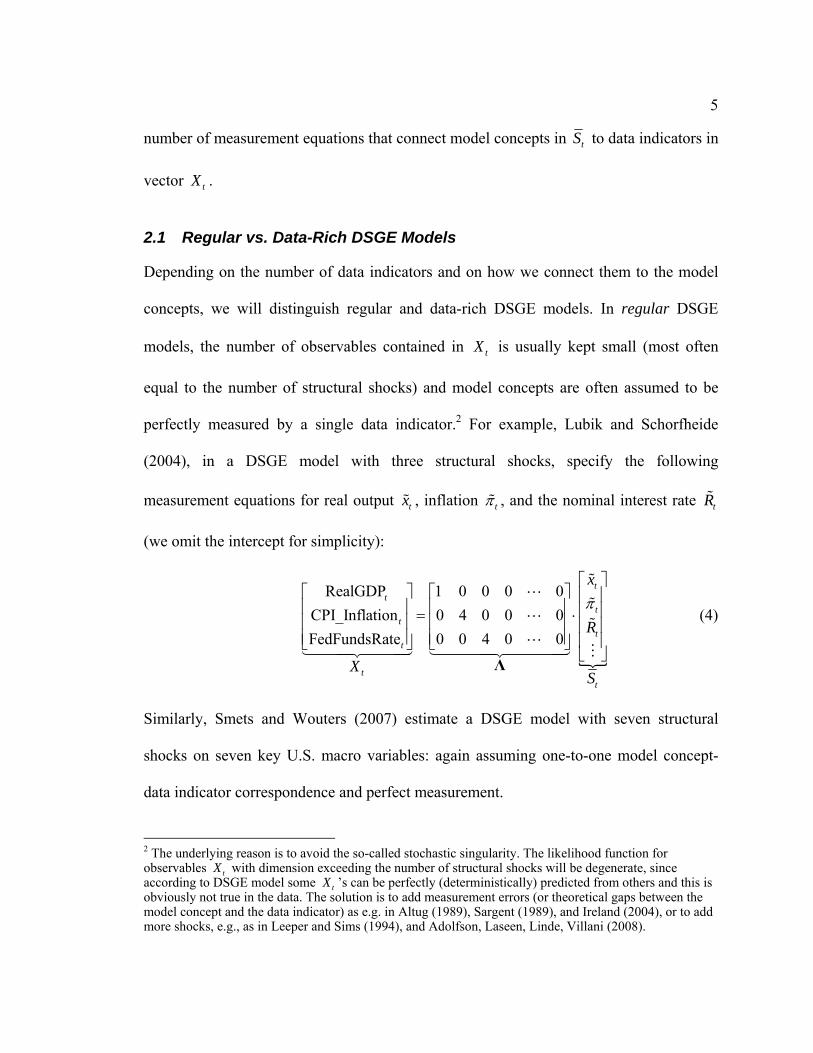
2.1 Regular vs. Data-Rich DSGE Models
Depending on the number of data indicators and on how we connect them to the model
concepts, we will distinguish regular and data-rich DSGE models. In regular DSGE
models, the number of observables contained in tX is usually kept small (most often
equal to the number of structural shocks) and model concepts are often assumed to be
perfectly measured by a single data indicator.2 For example, Lubik and Schorfheide
(2004), in a DSGE model with three structural shocks, specify the following
measurement equations for real output tx , inflation tπ , and the nominal interest rate tR
Similarly, Smets and Wouters (2007) estimate a DSGE model with seven structural
shocks on seven key U.S. macro variables: again assuming one-to-one model concept-
data indicator correspondence and perfect measurement.
2 The underlying reason is to avoid the so-called stochastic singularity. The likelihood function for observables tX with dimension exceeding the number of structural shocks will be degenerate, since according to DSGE model some tX ’s can be perfectly (deterministically) predicted from others and this is obviously not true in the data. The solution is to add measurement errors (or theoretical gaps between the model concept and the data indicator) as e.g. in Altug (1989), Sargent (1989), and Ireland (2004), or to add more shocks, e.g., as in Leeper and Sims (1994), and Adolfson, Laseen, Linde, Villani (2008).
6
Following an important contribution of Boivin and Giannoni (2006), data-rich
DSGE models relax these assumptions and allow for: (i) the presence of measurement
errors or, alternatively, of terms capturing the theoretical gap between a particular data
indicator and a model concept it is supposed to measure; (ii) multiple data indicators ,j tX
measuring the same model concept ,i tS , and (iii) many informational data series in tX
with an unknown link to specific model concepts that load on all DSGE model states (and
that may contain useful information about the state of the economy). We call the core
series FtX the part of tX in which each data indicator loads on a single model concept
,i tS only (although same ,i tS may have several data indicators measuring it):
F Ft t tX S e= +FΛ , (5)
where each row of FΛ contains just one non-zero element. We call the non-core series
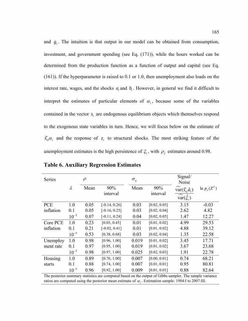
StX the remaining part of tX that is not supposed to measure any model concept and
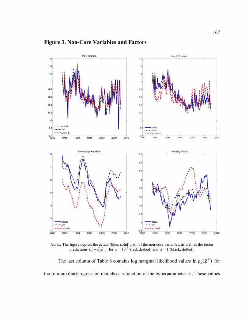
therefore loads freely on all DSGE model states:
S St t tX S e= +SΛ (6)
For example, in a simple closed-economy DSGE model of Lubik and Schorfheide (2004),
the core series might have been various measures of real output (e.g., real GDP, industrial
production), of inflation (e.g., CPI inflation, PCE deflator inflation) or of the nominal
interest rate; the non-core series might include exchange rates, real exports and imports,
stock returns and similar data indicators not related directly to any model concept. We
7
partition ,1 ,2⎡ ⎤= ⎣ ⎦F F FΛ Λ Λ conformably and use definition (3) to obtain the
measurement equation in the data-rich DSGE model for demeaned tX :
,1 ,2F Ft tS t St t
tt
X eS
X eeX
+⎡ ⎤ ⎡ ⎤⎡ ⎤= +⎢ ⎥ ⎢ ⎥⎢ ⎥
⎢ ⎥ ⎢ ⎥⎣ ⎦⎣ ⎦ ⎣ ⎦
F F
S
Λ D(θ) ΛΛ
Λ(θ)
, (7)
where the measurement errors te may be serially correlated, but uncorrelated across
different data indicators ( , Ψ R are diagonal):
1 , ~ ( , )t t t te e v v iid N−= +Ψ 0 R . (8)
So the state-space representation of the data-rich DSGE model consists of transition
equation (2) and measurement equations (7)-(8).
2.2 Environment
In this chapter, we use a relatively standard New Keynesian business cycle core that will
be shared by the data-rich and the regular DSGE models. It features capital as the factor
of production, nominal rigidities in price setting, and investment adjustment costs. The
real money stock enters households’ utility in additively separable fashion as in Walsh
(2003, Ch. 5), and Sidrauski (1967). In terms of a specific version of the model, we draw
upon the work of Aruoba and Schorfheide (2009) and their money-in-the-utility
specification.
The economy is populated by households, final and intermediate goods-producing
firms and a central bank (monetary authority). A representative household works,
consumes, saves, holds money balances and accumulates capital. It consumes the final
8
output manufactured by perfectly competitive final good firms. The final good producers
produce by combining a continuum of differentiated intermediate goods supplied by
monopolistically competitive intermediate goods firms. To manufacture their output,
intermediate goods producers hire labor and capital services from households. Also,
when optimizing their prices, intermediate goods firms face the nominal price rigidity a la
Calvo (1983), and those firms that are unable to re-optimize may index their price to
lagged inflation. Monetary policy is conducted by the central bank setting the one-period
nominal interest rate on public debt via a Taylor-type interest rate feedback rule. Given
the interest rate, the central bank supplies enough nominal money balances to meet
equilibrium demand from households.
Our DSGE model is more elaborate than the basic three-equation model used in
Woodford (2003), but is “lighter” than the models in Smets and Wouters (2003, 2007)
and Christiano, Eichenbaum and Evans (2005): it abstracts from wage rigidities, habit
formation in consumption and variable capital utilization.
2.2.1 Households
In our environment, there is a continuum of households indexed by [0;1]j∈ . Each
household maximizes the following utility function:
(1 )
0 1 (1 )0
( )( ( )) ( ) ,1
m
t t tt t
t m t
m jAE U x j Ah jZ P
ν
α
χβν
−∞
−= ∗
⎧ ⎫⎡ ⎤⎪ ⎪− +⎨ ⎬⎢ ⎥− ⎣ ⎦⎪ ⎪⎩ ⎭∑ (9)
which is additively separable in consumption ( )tx j , labor supply ( )th j and real money
balances ( )t tm j P . Here β stands for the discount factor, A denotes disutility of labor,
9
mν controls the elasticity of money demand and tχ is an aggregate preference shifter that
affects households’ marginal utility from holding real money balances.3 The law of
motion for tχ is:
21 , ,ln (1 ) ln ln , where ~ (0, )t t t t Nχ χ χ χ χχ ρ χ ρ χ ε ε σ∗ −= − + + (10)
We assume that households are able to trade on a complete set of Arrow-Debreu
(A-D) securities, which are contingent on all aggregate and idiosyncratic events ω∈Ω in
the economy. Let 1( )( )ta j ω+ denote the quantity of A-D securities (that pay 1 unit of
consumption in period 1t + in the event ω ) acquired by household j at time t at real
price 1, ( )t tq j+ . Then household j ’s budget constraint in nominal terms is given by:
1 1 1, 1
1
( ) ( ) ( ) ( ) ( ) ( )( )
( ) ( ) ( ) ( ) ( )
t t t t t t t t t t
kt t t t t t t t t t t t t
P x j Pi j b j m j P q j a j d
PW h j PR k j R b j m j Pa j T
ω ω+ + + +Ω
−
+ + + + =
= + +Π + + + −
∫ (11)
where tP is the period t price of the final good, ( )ti j is investment, ( ) and ( )t tb j m j are
government bond and money holdings, tR is the gross nominal interest rate on
government bonds, tW and ktR are the real wage and real return on capital earned by
households, tΠ stands for profits from owning the firms, and tT is the nominal amount of
lump-sum taxes paid. Households also accumulate capital ( )tk j according to the
following law of motion:
3 As in Aruoba and Schorfheide (2009), scaling ( )t tm j P by a factor 1 (1 )A Z α−
∗ can be viewed as re-parameterization of tχ , in which the steady-state money velocity remains constant when we move around A and Z∗ .
10
11
( )( ) (1 ) ( ) 1 ( ),( )
tt t t
t
i jk j k j S i ji j
δ+−
⎡ ⎤⎛ ⎞= − + −⎢ ⎥⎜ ⎟
⎢ ⎥⎝ ⎠⎣ ⎦ (12)
where δ is the depreciation rate and ( )S i is an adjustment cost function satisfying
(1) 0S = , (1) 0S ′ = and (1) 0S ′′ > .
The problem of each household j is to maximize the utility function (9) subject
to budget constraint (11) and capital accumulation equation (12) for all t . Associate
Lagrange multipliers ( )t jλ and ( )tQ j with constraints (11) and (12), respectively. The
first-order conditions are provided in Appendix A1. We do not take the first-order
conditions with respect to A-D securities holdings 1( )ta j+ explicitly, because we make
use of the result in Erceg, Henderson and Levin (2000). This result says that under the
assumption of complete markets for A-D securities and under the additive separability of
labor and money balances in households’ utility, the equilibrium price of A-D securities
will be such that optimal consumption will not depend on idiosyncratic shocks. Hence, all
households will share the same marginal utility of consumption, and the Lagrange
multiplier ( )t jλ will also be the same across all households: ( )t tjλ λ= , all j and t. This
implies that in equilibrium all households will choose the same consumption, money and
bond holdings, investment and capital. Note that we don’t have wage rigidity in this
model: therefore, the choice of optimal labor will also be same. Therefore we can safely
drop index j from all household-related conditions and variables and proceed
accordingly.
11
Let us define the stochastic discount factor 1|pt t+Ξ that the firms – whose behavior
we are going to describe shortly – will use to value streams of future profits:
1 11|
1
( ) 1( )
p t tt t
t t t
U xU x
λλ π+ +
++
′Ξ = =
′, (13)
where 1t t tP Pπ −= denotes final good price inflation.
2.2.2 Final Good Firms
There is single final good tY in our economy manufactured by combining a continuum of
intermediate goods ( )tY i indexed by [0;1]i∈ according to the following production
function:
(1 )1 1
1
0
( ) ,t tY Y i diλ
λ
+
+⎛ ⎞
= ⎜ ⎟⎝ ⎠∫ (14)
where the elasticity of substitution between any goods i and j is 1 λλ+ .
The final good firms purchase intermediate goods in the market, package them
into a composite final good, and sell the final good to households. These firms are
perfectly competitive and maximize one-period profits subject to production function
(14), taking as given intermediate goods prices ( )tP i and own output price tP :
1
0
(1 )1 11
0
max ( ) ( ), ( )
s.t. ( )
t t t t
t t
t t
PY P i Y i diY Y i
Y Y i diλ
λ
+
+
−
⎛ ⎞= ⎜ ⎟⎝ ⎠
∫
∫ (15)
The first-order condition leads to the optimal demand for good i:
12
(1 )
( )( ) .tt t
t
P iY i YP
λλ+
−⎛ ⎞
= ⎜ ⎟⎝ ⎠
(16)
Since final good firms are perfectly competitive and there is free entry, they earn zero
profits in equilibrium, which, together with optimal demand (16), yields the price of the
final good:
1 1
0
( ) .t tP P i diλ
λ
−−⎡ ⎤
= ⎢ ⎥⎣ ⎦∫ (17)
2.2.3 Intermediate Goods Firms
Our economy is populated by a continuum of intermediate goods firms. Each
intermediate goods firm i uses the following technology to produce its output:
(1 )( ) max ( ) ( ) ,0 ,t t t tY i Z K i H i Fα α−= − (18)
where ( )tK i is the amount of capital that the firm i rents from households, ( )tH i is the
amount of labor input and tZ is the level of neutral technology evolving according to the
law of motion:
21 , ,ln (1 ) ln ln , where ~ (0, ).t Z Z t Z t Z t ZZ Z Z Nρ ρ ε ε σ∗ −= − + + (19)
Parameter α stands for the capital share of production, while parameter F controls the
amount of fixed costs in production that guarantee that the firm’s economic profits will
be zero in the steady state. Unlike with the final good producers, we do not allow for free
entry or exit on the part of the intermediate goods firms.
13
All intermediate goods producers are monopolistically competitive, in that they
take all factor prices ( tW and ktR ), as well as the prices of other firms, as given, but can
optimally choose their own price ( )tP i subject to optimal demand (16) for good i from
final good firms. Intermediate firms solve a two-stage optimization problem.
In the first stage, the firms hire capital and labor from households to minimize
total nominal costs:
( ), ( )
(1 )
min ( ) ( )
s.t. ( ) max ( ) ( ) ,0t t
kt t t t t tK i H i
t t t t
PW H i PR K i
Y i Z K i H i Fα α−
+
= − (20)
Assuming interior solution, optimality conditions imply ( ( )t iη is the Lagrange multiplier
attached to (18)):
( ) ( )(1 ) ( ) ( )t t t t t t tPW i P i Z K i H iα αη α −= −
1 1( ) ( ) ( ) ( )kt t t t t t tPR i P i Z K i H iα αη α − −=
Take the ratio of two conditions to obtain:
( )( ) 1
t tk
t t
K i WH i R
αα
=−
(21)
If we define aggregate capital stock 1
0
( )t tK K i di= ∫ and aggregate labor 1
0
( )t tH H i di= ∫ ,
integrating both sides of (21) yields:
1
tt tk
t
WK HR
αα
=−
(22)
14
Now we can factorize total real variable cost ( )tVC i into real marginal cost tMC
and the variable part of firm i ’s output var (1 )( ) ( ) ( )t t t tY i Z K i H iα α−= :
var( ) ( ) ( )1( ) ( ) ( )( ) ( ) ( )
k kt t tt t t t t t t
t t t t
K i K i K iVC i W R H i W R Y iH i H i Z H i
α−⎛ ⎞ ⎛ ⎞ ⎛ ⎞
= + = +⎜ ⎟ ⎜ ⎟ ⎜ ⎟⎝ ⎠ ⎝ ⎠ ⎝ ⎠
(23)
Plugging in the optimal capital labor ratio (21), real marginal cost tMC turns out to be
For convenience, we collect all DSGE model parameters in the vector θ and stack
all innovations in vector , , , ,[ , , , ]t Z t t g t R tχε ε ε ε ε ′= . We then derive a log-linear
approximation to the system of equilibrium conditions (summarized in Appendix A4 and
A5) around its deterministic steady state. The resulting linear rational expectations
system is solved by the method described in Sims (2002).
19
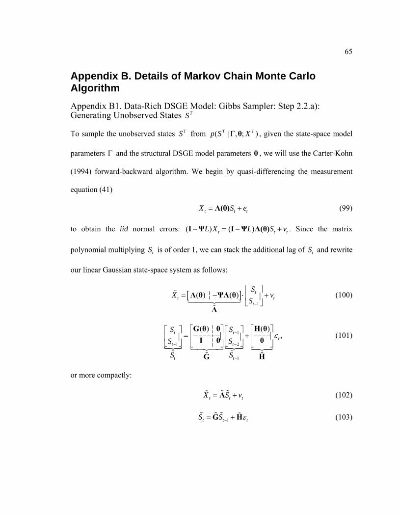
3 Econometric Methodology In this section, we first provide the details on a Markov Chain Monte Carlo (MCMC)
algorithm to estimate the data-rich DSGE model, including the choice of the prior for
factor loadings. Second, we present the novel speed-up suggested by Jungbacker and
Koopman (2008), which enhances the speed of our Bayesian estimation procedure.
3.1 Estimation of the Data-Rich DSGE Model
As discussed in the previous section, the state-space representation of our data-rich DSGE
model consists of a transition equation of model states tS and a set of measurement
equations relating the states4 to data tX :
11 1 1t t t
N N N NN N N
S Sε ε
ε−
× ×× × ×
= +G(θ) H(θ) (40)
1 1 1t t t
J NJ N J
X S e×× × ×
= +Λ(θ) (41)
1 ,t t te e v−= +Ψ (42)
where ~ ( , )t iid Nε 0 Q(θ) , ~ ( , )tv iid N 0 R and where Q(θ) , R and Ψ are assumed
diagonal. An essential feature of a data-rich framework is that the panel dimension of
data set J is much higher than the number of DSGE model states N . For convenience,
collect state-space matrices from the measurement equation into , ,Γ = Λ(θ) Ψ R and
DSGE states-factors into 1 2, , ,TTS S S S= … . Because of the normality of structural
4 In measurement equations (41) we keep only the non-redundant state variables of a DSGE model. Because some of the DSGE states are merely linear combinations of the other states, one can interpret this as minimum-state-variable approach in the spirit of McCallum (1983, 1999, 2003). Here, though, the main rationale is to avoid multicollinearity on the right hand side of (41). We always set the corresponding factor loadings in Λ equal to zero.
20
shocks tε and measurement error innovations tv , system (40)-(42) is a linear Gaussian
state-space model and the likelihood function of data ( | , )Tp X Γθ can be evaluated using
a Kalman filter.
Following Boivin and Giannoni (2006), we use Bayesian techniques to estimate
the unknown model parameters ( , )Γθ . We combine prior ( , ) ( | ) ( )p p pΓ = Γθ θ θ with the
likelihood function ( | , )Tp X Γθ to obtain the posterior distribution of parameters given
data:
( | , ) ( , )( , | )( | , ) ( , )
TT
T
p X pp Xp X p d d
Γ ΓΓ =
Γ Γ Γ∫θ θθ
θ θ θ (43)
We use Markov Chain Monte Carlo (MCMC) method to estimate posterior density
( , | )Tp XΓθ by constructing a Markov chain with the property that its limiting invariant
distribution is our posterior distribution. Similarly to Boivin and Giannoni (2006), the
Markov chain is constructed by the Gibbs sampling method with a Metropolis-within-
Gibbs step to generate draws from the posterior distribution ( , | )Tp XΓθ and to compute
the approximations to posterior means and covariances of parameters of interest.
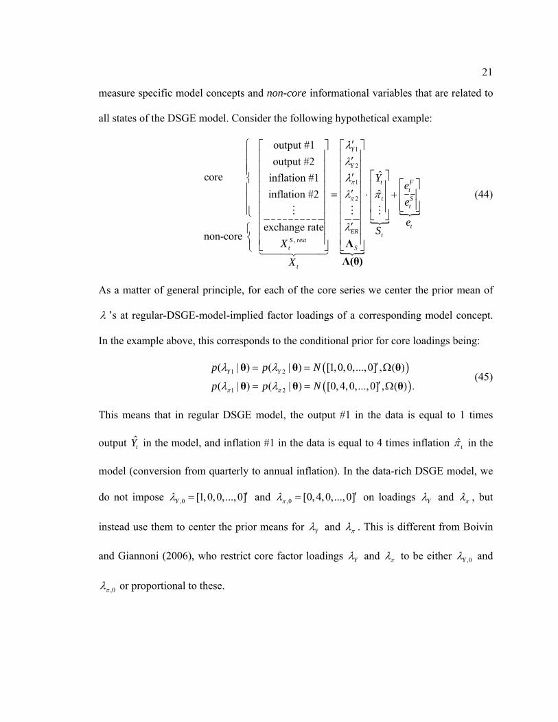
But before we turn to describing the Gibbs sampler, we must elaborate on how we
connect the DSGE model states to data indicators. This is important, because, unlike in
Boivin and Giannoni (2006), the link is primarily through the prior on factor loadings
Λ(θ) . The priors for the rest of the parameters (θ , Ψ and R ) are discussed in detail in
the section “Empirical Results: Priors” below. Recall that we have core data series that
21
measure specific model concepts and non-core informational variables that are related to
all states of the DSGE model. Consider the following hypothetical example:
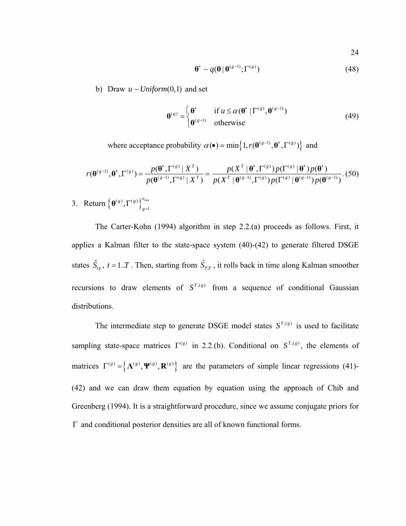
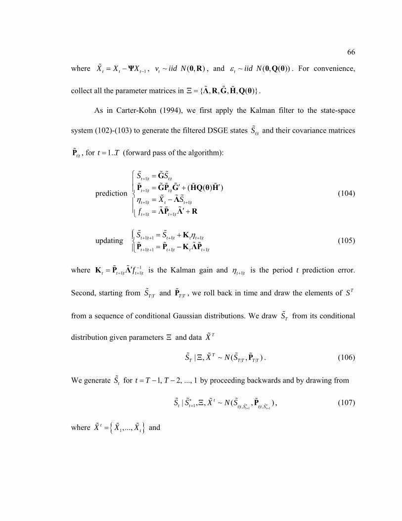
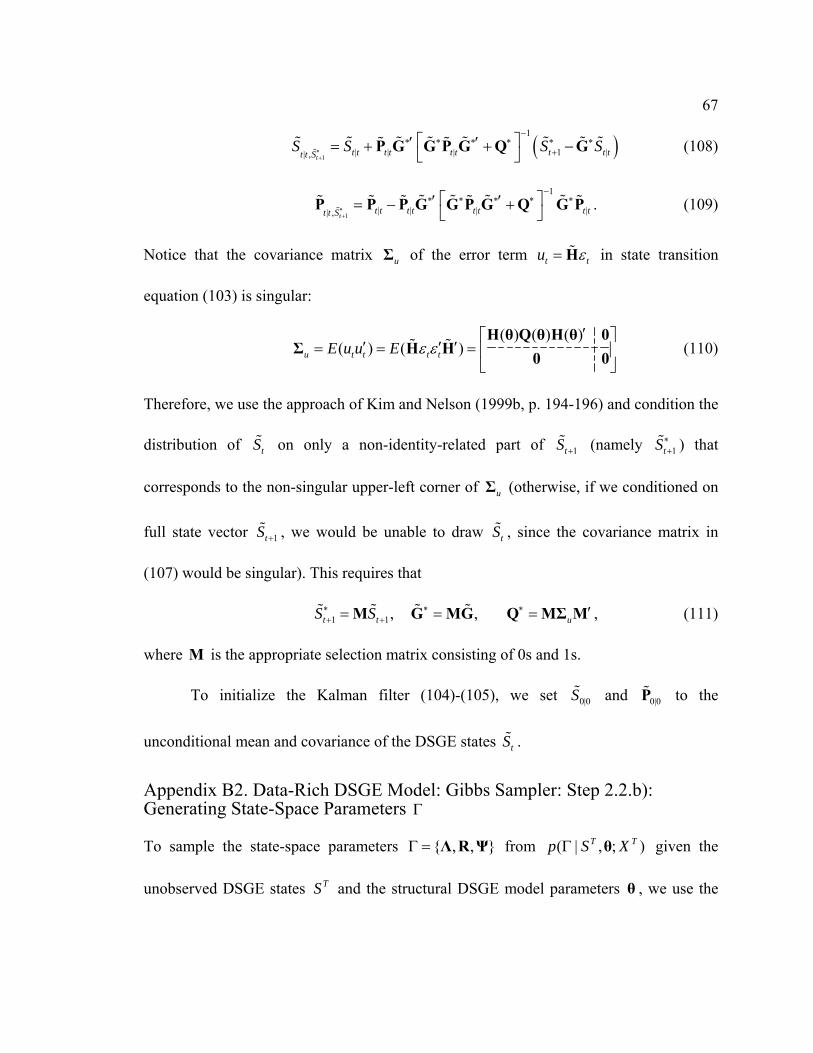
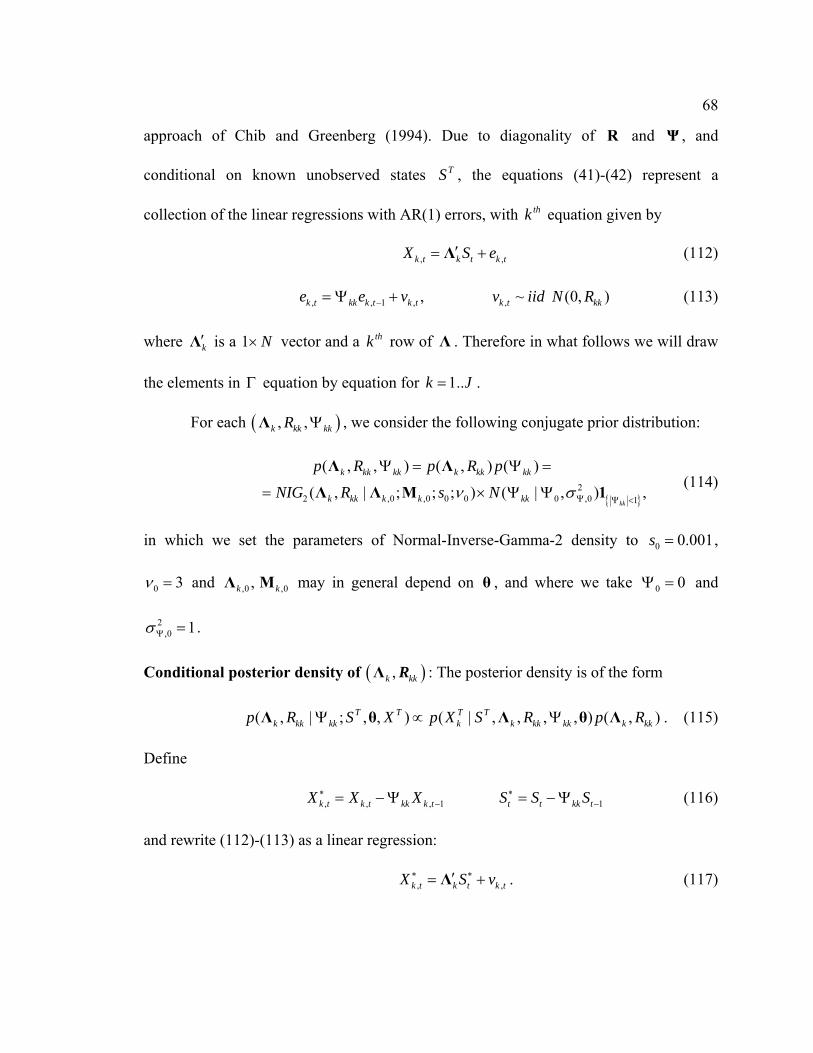
The Carter-Kohn (1994) algorithm in step 2.2.(a) proceeds as follows. First, it
applies a Kalman filter to the state-space system (40)-(42) to generate filtered DSGE
states |ˆ
t tS , 1..t T= . Then, starting from |ˆ
T TS , it rolls back in time along Kalman smoother
recursions to draw elements of ,( )T gS from a sequence of conditional Gaussian
distributions.
The intermediate step to generate DSGE model states ,( )T gS is used to facilitate
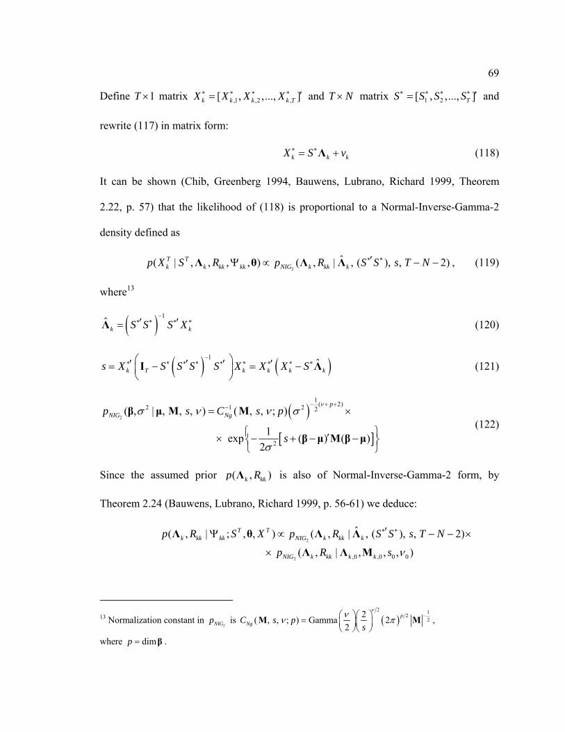
sampling state-space matrices ( )gΓ in 2.2.(b). Conditional on ,( )T gS , the elements of
matrices ( ) ( ) ( ) ( ), ,g g g gΓ = Λ Ψ R are the parameters of simple linear regressions (41)-
(42) and we can draw them equation by equation using the approach of Chib and
Greenberg (1994). It is a straightforward procedure, since we assume conjugate priors for
Γ and conditional posterior densities are all of known functional forms.
25
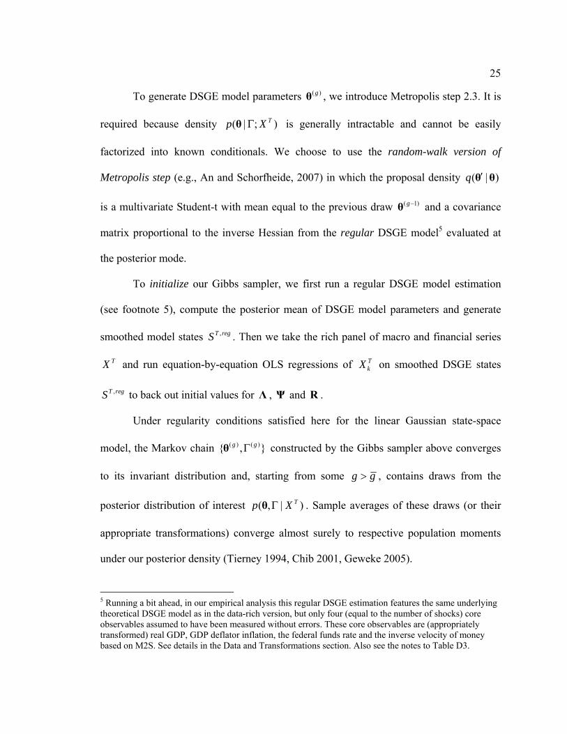
To generate DSGE model parameters ( )gθ , we introduce Metropolis step 2.3. It is
required because density ( | ; )Tp XΓθ is generally intractable and cannot be easily
factorized into known conditionals. We choose to use the random-walk version of
Metropolis step (e.g., An and Schorfheide, 2007) in which the proposal density ( | )q ′θ θ
is a multivariate Student-t with mean equal to the previous draw ( 1)g−θ and a covariance
matrix proportional to the inverse Hessian from the regular DSGE model5 evaluated at
the posterior mode.
To initialize our Gibbs sampler, we first run a regular DSGE model estimation
(see footnote 5), compute the posterior mean of DSGE model parameters and generate
smoothed model states ,T regS . Then we take the rich panel of macro and financial series
TX and run equation-by-equation OLS regressions of TkX on smoothed DSGE states
,T regS to back out initial values for Λ , Ψ and R .
Under regularity conditions satisfied here for the linear Gaussian state-space
model, the Markov chain ( ) ( ) , g gΓθ constructed by the Gibbs sampler above converges
to its invariant distribution and, starting from some g g> , contains draws from the
posterior distribution of interest ( , | )Tp XΓθ . Sample averages of these draws (or their
appropriate transformations) converge almost surely to respective population moments
under our posterior density (Tierney 1994, Chib 2001, Geweke 2005).
5 Running a bit ahead, in our empirical analysis this regular DSGE estimation features the same underlying theoretical DSGE model as in the data-rich version, but only four (equal to the number of shocks) core observables assumed to have been measured without errors. These core observables are (appropriately transformed) real GDP, GDP deflator inflation, the federal funds rate and the inverse velocity of money based on M2S. See details in the Data and Transformations section. Also see the notes to Table D3.
26
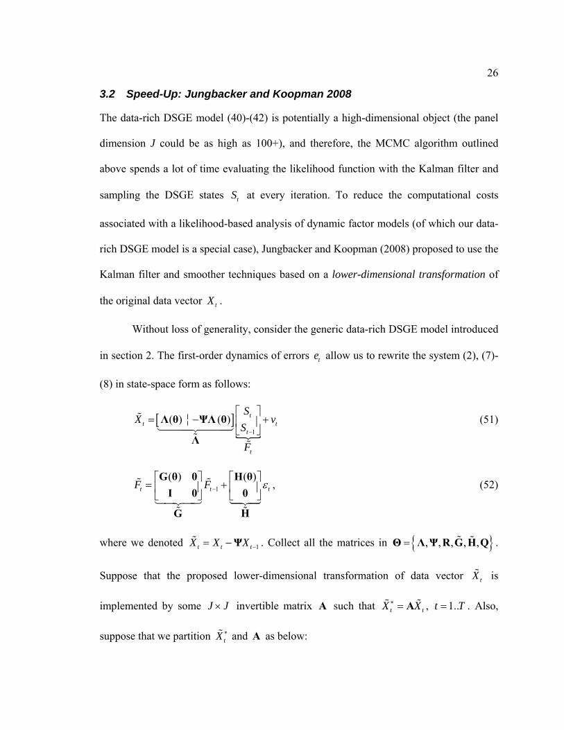
3.2 Speed-Up: Jungbacker and Koopman 2008
The data-rich DSGE model (40)-(42) is potentially a high-dimensional object (the panel
dimension J could be as high as 100+), and therefore, the MCMC algorithm outlined
above spends a lot of time evaluating the likelihood function with the Kalman filter and
sampling the DSGE states tS at every iteration. To reduce the computational costs
associated with a likelihood-based analysis of dynamic factor models (of which our data-
rich DSGE model is a special case), Jungbacker and Koopman (2008) proposed to use the
Kalman filter and smoother techniques based on a lower-dimensional transformation of
the original data vector tX .
Without loss of generality, consider the generic data-rich DSGE model introduced
in section 2. The first-order dynamics of errors te allow us to rewrite the system (2), (7)-
(8) in state-space form as follows:
[ ]1
( ) ( ) tt t
t
t
SX v
S
F−
⎡ ⎤= − +⎢ ⎥
⎣ ⎦Λ θ ΨΛ θ
Λ
(51)
1
( ) ( )t t tF F ε−
⎡ ⎤ ⎡ ⎤= +⎢ ⎥ ⎢ ⎥⎣ ⎦ ⎣ ⎦
G θ 0 H θI 0 0
HG
, (52)
where we denoted 1t t tX X X −= −Ψ . Collect all the matrices in , , , , ,=Θ Λ Ψ R G H Q .
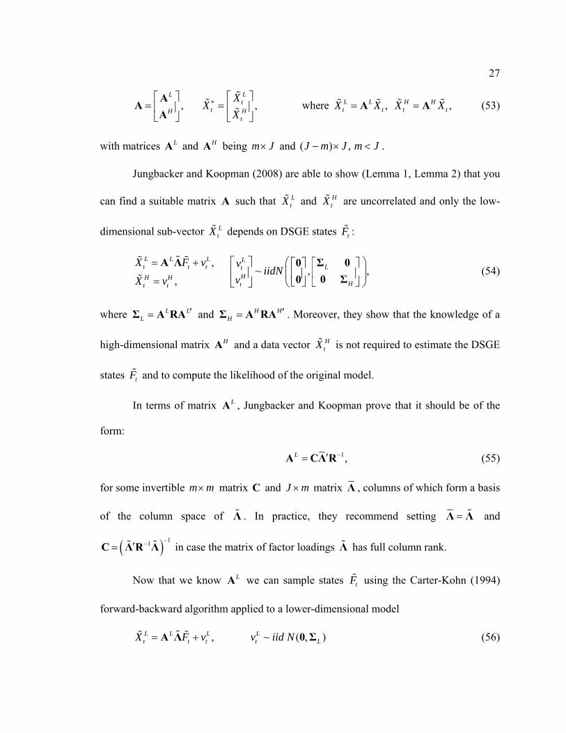
Suppose that the proposed lower-dimensional transformation of data vector tX is
implemented by some J J× invertible matrix A such that t tX X∗ = A , 1..t T= . Also,
suppose that we partition tX ∗ and A as below:
27
, , where , ,LL
L L H Htt t t t tHH
t
XX X X X X
X∗ ⎡ ⎤⎡ ⎤
= = = =⎢ ⎥⎢ ⎥⎣ ⎦ ⎣ ⎦
AA A A
A (53)
with matrices LA and HA being m J× and ( ) ,J m J m J− × < .
Jungbacker and Koopman (2008) are able to show (Lemma 1, Lemma 2) that you
can find a suitable matrix A such that LtX and H
tX are uncorrelated and only the low-
dimensional sub-vector LtX depends on DSGE states tF :
,
,
L L Lt t t
H Ht t
X F v
X v
= +
=
A Λ ~ , ,
LLt
HHt
viidN
v⎛ ⎞⎡ ⎤ ⎡ ⎤⎡ ⎤⎜ ⎟⎢ ⎥ ⎢ ⎥⎢ ⎥⎣ ⎦ ⎣ ⎦⎣ ⎦ ⎝ ⎠
Σ 000 Σ0
(54)
where L LL
′=Σ A RA and H HH
′=Σ A RA . Moreover, they show that the knowledge of a
high-dimensional matrix HA and a data vector HtX is not required to estimate the DSGE
states tF and to compute the likelihood of the original model.
In terms of matrix LA , Jungbacker and Koopman prove that it should be of the
form:
1,L −′=A CΛ R (55)
for some invertible m m× matrix C and J m× matrix Λ , columns of which form a basis
of the column space of Λ . In practice, they recommend setting =Λ Λ and
( ) 11 −−′=C Λ R Λ in case the matrix of factor loadings Λ has full column rank.
Now that we know LA we can sample states tF using the Carter-Kohn (1994)
forward-backward algorithm applied to a lower-dimensional model
, ~ ( , )L L L Lt t t t LX F v v iid N= +A Λ 0 Σ (56)
28
1 , ~ ( , ( ))t t t tF F iid Nε ε−= +G H 0 Q θ . (57)
We can also compute the log-likelihood of data ( | )L X Θ as
1
1
1 ˆ ˆ( | ) ( | ) log ,2 2
TL
t ttL
TL X c L X v v−
=
′= + − − ∑R
Θ Θ RΣ
(58)
where 12 ( ) log(2 )c J m T π= − − and ( )1 1
t t tv X X− −⎡ ⎤′ ′= − ⎣ ⎦Λ Λ R Λ Λ R . The term
( | )LL X Θ is the log-likelihood of the transformed data evaluated by using a Kalman
filter during the forward pass of the Carter-Kohn algorithm on the low-dimensional
model (56)-(57).
In the ensuing empirical analysis of a data-rich DSGE model, we have applied the
Jungbacker-Koopman algorithm presented in this section to improve the speed of
computations. To get a sense of CPU time gains, we have also estimated the model –
though on fewer draws – without the speed-up and have found that the “improved”
estimation of the data-rich DSGE model runs 2.5 times faster. The CPU gains reported by
Jungbacker and Koopman (2008) for a dynamic factor model of a size similar to our data-
rich DSGE model are about 11 times faster. Differences in time savings are due to the
significant chunk of time that it takes to solve numerically the underlying DSGE model in
the data-rich DSGE model estimation, a step absent in the DFM estimation and not
affected by the Jungbacker-Koopman speed-up.
29
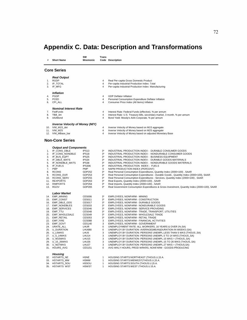
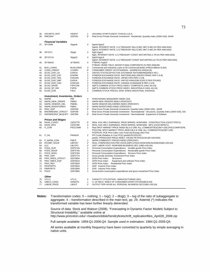
4 Data and Transformations To estimate the data-rich DSGE model, we employ a large panel of U.S. quarterly
macroeconomic and financial time series compiled by Stock and Watson (2008).6 The
panel covers 1959:Q1 – 2006:Q4, however, our sample in this chapter spans only
1984:Q1 – 2005:Q4. We focus on this later period primarily for two reasons: (i) to avoid
dealing with the issue of the Great Moderation7; and (ii) to concentrate on a period with a
relatively stable monetary policy regime.
Our data set consists of 12 core series that measure specific DSGE model
concepts and 77 non-core informational series that load on all DSGE states and may
contain useful information about the aggregate state of the economy. The core series
include three measures of real output (real GDP, the index of total industrial production
and the index of industrial production: manufacturing), three measures of price inflation
(GDP deflator inflation, personal consumption expenditure (PCE) deflator inflation, and
CPI inflation), three indicators of the nominal interest rates (the federal funds rate, the 3-
month T-bill rate and the yield on AAA-rated corporate bonds), and three series
measuring the inverse velocity of money (IVM based on the M1 aggregate and the M2
aggregate and IVM based on the adjusted monetary base). The 77 non-core series include
the measures of real activity, labor market variables, housing indicators, prices and
6 The data set is available online at: http://www.princeton.edu/~mwatson/ddisk/hendryfestschrift_replicationfiles_April28_2008.zip 7 The “Great Moderation” refers to a decline in the volatility of output and inflation observed in the U.S. since the mid-1980s until the recent financial crisis. For evidence and implications, please see Bernanke (2004), Stock and Watson (2002c), Kim and Nelson (1999a), and McConnell and Perez-Quiros (2000). The last two papers argue that a break in the volatility of U.S. GDP growth occurred in 1984:Q1.
30
stocks, stock returns) and, together with appropriate transformations to eliminate trends,
are described in Appendix C.
Most of the core series are computed based on the raw indicators from Stock and
Watson (2008) database and from the Fred-II database8 maintained by the Federal
Reserve Bank of St. Louis (database mnemonics are in italics). To obtain three measures
of real per-capita output, we take real GDP (SW2008::GDP251), total industrial
production (SW2008::IPS10) and industrial production in the manufacturing sector
(SW2008::IPS43), and divide each series by the civilian non-institutional population
(Fred-II::CNP16OV). We then take the natural logarithm and extract the linear trend by
an OLS regression. The resulting detrended series are multiplied by 100 to convert them
to percentage deviations from respective means. The inflation measures are computed as
the first difference of the natural logarithm of the GDP deflator (SW2008::GDP272A), of
the PCE deflator (SW2008::GDP273A), and of the Consumer Price Index – All Items
(SW2008::CPIAUCSL), all multiplied by 400 to get to the annualized percentages. Our
indicators of the nominal interest rate are (i) the effective federal funds rate
(SW2008::FYFF), (ii) the 3-month U.S. Treasury bill rate in the secondary market
(SW2008::FYGM3) and (iii) the yield on Moody’s AAA-rated corporate bonds
(SW2008::FYAAAC). We use a simple 3-month average to obtain quarterly annualized
interest rates from monthly raw data.
To generate the appropriate inverse money velocities, we take three monetary
aggregates: the sweep-adjusted money stock M1 (CDJ::M1S), the sweep-adjusted money
8 The Fred-II database is available online at: http://research.stlouisfed.org/fred2/
31
stock M2 (CDJ::M2S) and the monetary base adjusted for changes in reserve
requirements (SW2008::FMFBA). The sweep-adjusted stocks M1S and M2S are provided
by Cynamon, Dutkowsky and Jones (2006)9 and correct the distortionary impact (on the
conventional measures M1 and M2) of the financial innovation that started in the early
1990s. These distortions take the form of underreporting of actual transactions balances
and arise because of retail sweep programs and commercial demand deposit sweep
programs, in which U.S. banks move a portion of funds from their customer demand
deposits or other checkable deposits into instruments with zero reserve requirements.
Since our DSGE model does not have any explicit open- economy context, we further
adjust the monetary base FMFBA by deducting the amount of U.S. dollar currency held
physically outside the United States.10 We take M1S, M2S and the adjusted FMFBA,
divide each series by the nominal GDP (Fred-II::GDP) to obtain the respective inverse
velocities of money. For each IVM, we take the natural logarithm of the M/GDP ratio
and scale it by 100. Finally, we remove the linear deterministic trend from the IVM based
on M1S.
Because measurement equations (41) are modeled without intercepts, we estimate
the data-rich DSGE model on a demeaned data set. Also, in line with standard practice in
the factor literature, we standardize each time series so that its sample variance is equal to
unity (however, we do not scale the core series when estimating the data-rich DSGE
model).
9 Sweep-adjusted money stocks are available online at: http://www.sweepmeasures.com. 10 Federal Reserve Board: Flow of Funds Accounts of the United States: Z.1 Statistical Release for March 12, 2009 (available at http://www.federalreserve.gov/releases/z1/20090312/). Table L.204 “Checkable Deposits and Currency”, line 23 (Rest of the world: Currency), unique identifier: Z1/Z1/FL263025003.Q
32
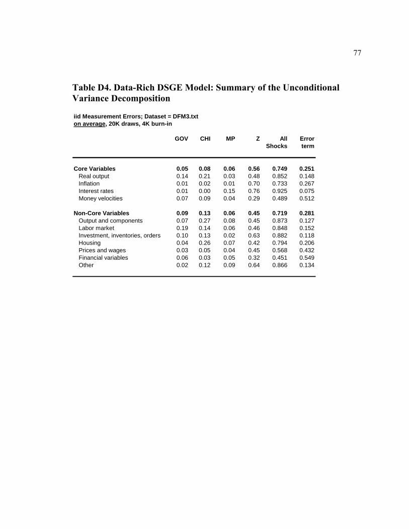
5 Empirical Results In this section, we conduct the empirical analysis of the regular and the data-rich DSGE
model. We begin by discussing the choice of the prior distributions of model parameters
and then describe the posterior estimates of deep structural parameters in both models.
Second, we compare the estimated DSGE state variables from our data-rich and from the
regular DSGE model. Finally, we explore the differences that the two models imply
about the sources of business cycle fluctuations and about the propagation of structural
innovations, notably the monetary policy and technology shocks, to the measures of real
output, inflation, interest rates and the real money balances.
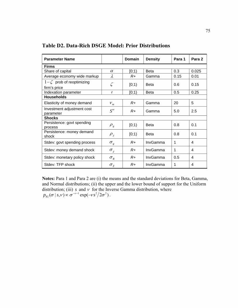
5.1 Priors
Since we estimate the regular DSGE model (130) and the data-rich DSGE model (40)-
(42) using Bayesian techniques, we have to provide prior distributions for both models’
parameters.
In our data-rich DSGE model, we have two groups of parameters: state-space
model parameters comprising matrices Λ , Ψ and R , and deep structural parameters θ
of an underlying DSGE model. The prior for the state-space matrices is elicited
differently for the core and the non-core data indicators contained in tX . Let kΛ and kkR
be the factor loadings and a variance of the measurement error innovation for the kth
measurement equation, 1..k J= .
Regarding the non-core measurement equations, the prior for ( ),k kkRΛ and for
kkΨ is defined as follows. Similarly to Boivin and Giannoni (2006) and Kose, Otrok and
33
Whiteman (2008), we assume a joint Normal-InverseGamma prior distribution for
( ),k kkRΛ so that 2 0 0~ ( , )kkR IG s ν with location parameter 0 0.001s = and degrees of
freedom 0 3ν = , and the prior mean of factor loadings is centered around the vector of
zeros | ~k kkRΛ 1,0 0( , )k kkN R −Λ M with ,0k =Λ 0 and 0 N=M I . The prior for the kth
measurement equation’s autocorrelation kkΨ , all k , is (0,1)N . We are making it
perfectly tight, however, because there could be data series with stochastic trends we seek
to capture with potentially highly persistent DSGE states-factors and not with highly
persistent measurement errors. This implies that all measurement errors are iid mean-zero
normal random variables.
In contrast, the prior distribution for the factor loadings in the core measurement
equations follows the scheme explained in example (44). Instead of hypothetical “output”
and “inflation” groups, we substitute four categories of the core series: real output,
inflation, the nominal interest rate, and the inverse velocity of money, with three specific
measures within each category, as described in the Data section. The joint prior
distribution is still Normal-Inverse-Gamma ,0 0 0( , , , )k os νΛ M , but now, for each of the
core series, the prior mean of the factor loadings ,0kΛ is centered at the regular-DSGE-
model-implied factor loadings of a corresponding DSGE model variable (real output tY ,
inflation ˆtπ , the nominal interest rate ˆtR or the inverse money velocity ˆ ˆ
t tM Y− ),
evaluated at the current draw of deep structural parameters θ . The covariance scaling
matrix 0M is assumed diagonal 0 ( ( ))diag=M Ω θ , where ( )Ω θ is the unconditional
34
covariance matrix of the DSGE model state variables evaluated at a current draw of θ .
0M is the same across all core measurement equations. This choice implies that the prior
will be tighter for the loadings on more volatile DSGE states. A similar approach is
pursued in Schorfheide, Sill and Kryshko (2010) reproduced as Chapter 3 in this
dissertation. The scale 0s and degrees of freedom 0ν are the same as for the parameters
in the non-core measurement equations above. Finally, as argued in section 3.1, we use a
degenerate prior for real GDP, GDP deflator inflation, the federal funds rate and the IVM
based on the M2S monetary aggregate.
Our choice of prior distribution for the deep structural parameters of a DSGE
model broadly follows Aruoba and Schorfheide (2009). We keep the same prior for the
regular and for the data-rich DSGE models that we estimate below. A subset of these
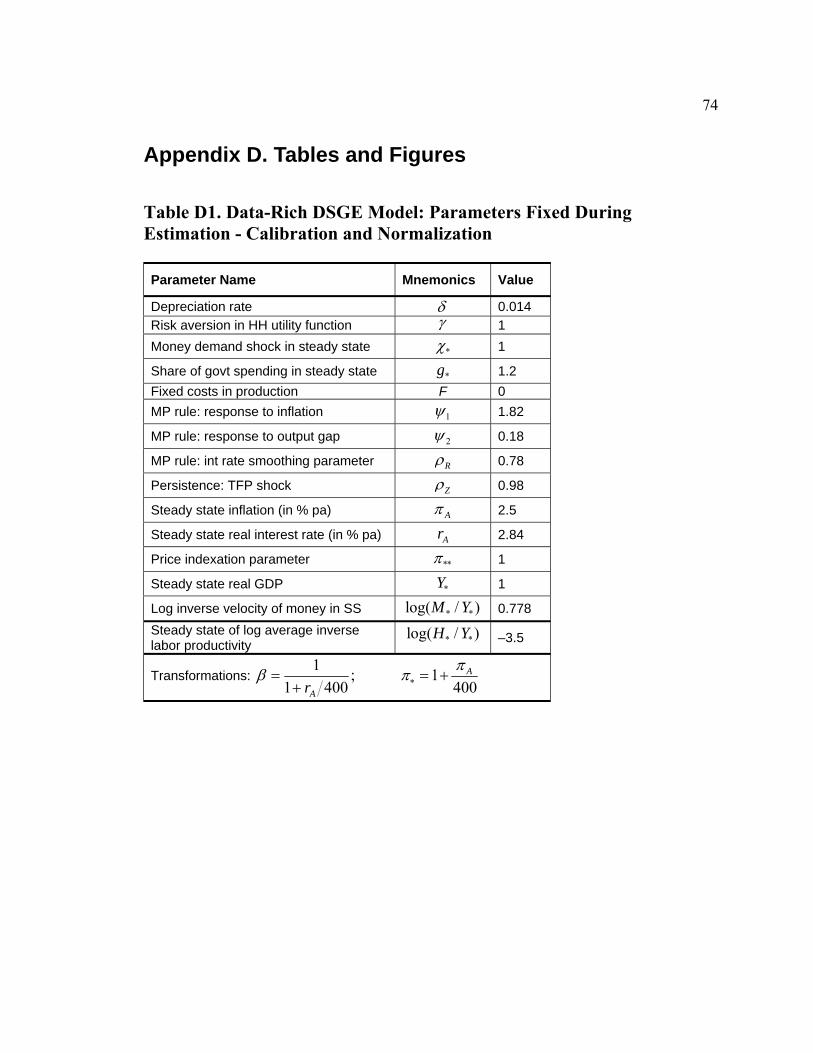
parameters that are fixed in estimation is reported in Table D1. We choose to have a
logarithmic utility of household consumption by fixing 1γ = . We set the depreciation
rate of capital δ to 0.014, which is the average quarterly ratio of the depreciation of fixed
assets to the stock of these fixed assets in 1959-2005 (NIPA-FAT11 for stocks, NIPA-
FAT13 for depreciation of fixed assets and consumer durables). The steady-state
annualized inflation rate Aπ is fixed at 2.5 percent – the average GDP deflator inflation
in our sample. We implicitly impose the Fischer equation and let the steady-state
annualized real interest rate Ar be equal to 2.84 percent. This value is obtained as the
average federal funds interest rate in our sample minus Aπ . Households’ discount factor
is therefore 1 (1 400)Arβ = + .
35
We also introduce several normalizations. We normalize to 1 the steady-state real
output Y∗ and steady-state money demand shock χ∗ . We use the average log inverse
velocity of money (log[M2S/GDP]) in our sample to pin down log( )M Y∗ ∗ . Finally, as in
Aruoba and Schorfheide (2009), we fix log( )H Y∗ ∗ to -3.5. This number is derived from
the average inverse labor productivity in the data. In our sample, on average a worker
produces roughly $33 of real GDP per hour. Hence, average H Y in the data is 1 33.
From the average share of government spending (consumption plus investment) in
nominal GDP, we calibrate g∗ to be 1.2.
We also want our data-rich DSGE model to be broadly consistent – in terms of the
conduct of monetary policy – with the other regular DSGE models estimated on post-
1983 data. Therefore, we shut down “data-richness” for a moment and estimate our
DSGE model on just three standard observables: real GDP, GDP deflator inflation and
the federal funds rate. The resulting estimates of the Taylor (1993) rule coefficients were:
1 1.82ψ = , 2 0.18ψ = and 0.78Rρ = . In the estimation of the data-rich DSGE model, we
set the policy rule coefficients to these values. This procedure is similar in spirit to Boivin
and Giannoni (2006), who assume that the policy rate tR is measured in the data by the
federal funds rate without an error. This assumption guarantees that the estimated
monetary policy rule coefficients will not drift far away from the conventional post-1983
values documented in the literature.
Despite detrending performed on all three measures of real per capita output, they
are still highly persistent. To strike a balance between the observed output persistence
36
and the need to have stationarity in the model, we fix the autocorrelation of the
technology shock Zρ at 0.98. In the intermediate goods-producing sector, we further
assume no fixed costs ( 0F = ) and the absence of static indexation for non-optimizing
firms ( 1π∗∗ = ).
The prior distributions for other parameters are summarized in Table D2. The
prior for the steady-state related parameters represents the view that the capital share of
α in a Cobb-Douglas production function of intermediate goods firms is about 0.3 and
that the average markup these firms charge is about 15 percent. The prior for the Calvo
(1983) probability ζ controlling nominal price rigidity is quite agnostic and spans the
range of values consistent with fairly rigid and fairly flexible prices. As in Del Negro and
Schorfheide (2008), the prior density for the price indexation parameter ι is close to
uniform on a unit interval. Parameter mν controlling the interest-rate elasticity of money
demand is a priori distributed according to a Gamma distribution with mean 20 and
standard deviation 5. The existing literature (e.g., Aruoba, Schorfheide 2009, Levin,
Onatsky, Williams and Williams 2005, and Christiano, Eichenbaum and Evans 2005)
documents fairly large estimates of the money demand elasticity ranging from 10 to 25.
The 90 percent interval for the investment adjustment cost parameter S ′′ spans values
that Christiano, Eichenbaum, Evans (2005) find when matching DSGE and vector
autoregression impulse response functions. The priors for the parameters determining the
exogenous shock processes are taken from Aruoba and Schorfheide (2009). They reflect
the belief that the money demand and government spending shocks are quite persistent.
37
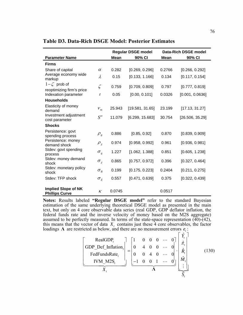
5.2 Posteriors: Regular vs. Data-Rich DSGE Model
Using the Gibbs sampler with the Metropolis step outlined in section 3.1, we estimate the
data-rich DSGE model. In addition, we have also estimated the regular DSGE model
using standard Bayesian techniques (Random Walk Metropolis-Hastings algorithm, see
An and Schorfheide, 2007). The underlying theoretical New Keynesian core is the same
as in the data-rich DSGE model. The difference comes in the measurement equation (41):
we keep only four core observable data series (real GDP, GDP deflator inflation, the
federal funds interest rate and the inverse velocity of money based on the M2S
aggregate), impose the factor loadings as in (130) and assume perfect measurement of all
four model concepts (see the notes to Table D3, p.76).
The only parameters of direct interest here are the deep structural parameters θ of
an underlying DSGE model, and we report the posterior means and 90 percent credible
intervals of these in the columns of Table D3. We find the capital share of output and the
average price markup to be in line with estimates from regular – few observables, perfect
measurement – DSGE estimation. We find little evidence of dynamic indexation by
intermediate goods firms in both versions of the model. The implied average duration of
nominal price contracts is about 1 (1 0.797)− = 4.9 quarters. On the one hand, this is
close to what Aruoba and Schorfheide (2009) find in their money-in-the-utility
specification of a DSGE model and what Del Negro and Schorfheide (2008) document
under the “standard” agnostic prior about nominal price rigidities (their Table 6, p. 1206).
On the other hand, this is much higher than the price contracts duration of about 3
quarters found by Smets and Wouters (2007) and Schorfheide, Sill and Kryshko (2010).
38
In the context of a data-rich DSGE model similar to ours, Boivin and Giannoni’s (2006)
estimates imply that the firms change prices very slowly – on average once per at least 7
quarters. The 4.9 quarters found in the data-rich version is quite higher than the duration
of price contracts documented for the regular DSGE model (1 (1 0.759) 4.15− =
quarters). The implication of this difference is that the implied slope of the New
Keynesian Phillips curve11 measuring the elasticity of current inflation to real marginal
costs (and to real output) falls from 0.0745 to 0.0517 as we move from the perfect
measurement, few observables to a richer data set in estimation of the same underlying
DSGE model. This means, for example, that the cost of disinflation associated with
achieving a 1 percent reduction in the rate of inflation at the expense of tolerating
negative real output growth, as predicted by the data-rich DSGE model, turns out to be
more sizable than the output cost of disinflation predicted by the traditional regular
DSGE model.
As anticipated, we have obtained a fairly high elasticity of money demand. Our
estimate of mν in the data-rich DSGE model case implies that a 100-basis-points increase
in the interest rate leads to a 3.2 percent decline in real money balances. A very large
estimate of the investment adjustment cost parameter (30.8 in data-rich versus 11.1 in the
11 We say implied slope because our underlying theoretical DSGE model is linearized around positive steady-state inflation rate ( 2.5%Aπ = ) and assumes the absence of static price indexation by the non-optimizing intermediate goods firms ( 1π∗∗ = ). This implies that we have a dynamic New Keynesian Phillips curve with additional lags of real marginal costs tMC . In a more conventional model where the non-optimizing intermediate goods firms index their prices to the steady-state inflation rate (π π∗∗ ∗= =
1 400Aπ= + ), the NK Phillps curve features only current marginal costs, the coefficient next to which mcγ we report:
1 1 2 1ˆ ˆ ˆ( )t t t t mc tE MCπ ππ γ π γ π γ− += + +
Note that (79) and (82) imply money demand equation12:
( )(1 )
1 1(1 )1 (1 )
1
.( )( 1)
m m
m
m
t t tt t
t t t t
m R AM EP U x R Z
ν νν
να
β χπ
−
+ +−−
∗ +
⎧ ⎫⎛ ⎞ ⎛ ⎞⎪ ⎪= = ⎨ ⎬⎜ ⎟ ⎜ ⎟′ − ⎝ ⎠⎝ ⎠ ⎪ ⎪⎩ ⎭ (85)
(2) Firms’ optimality conditions
1
tt tk
t
WK HR
αα
=−
(86)
( )1(1 )1 1
1
kt t
tt
W RMC
Z
ααα α
α α
−−⎛ ⎞ ⎛ ⎞= ⎜ ⎟ ⎜ ⎟−⎝ ⎠ ⎝ ⎠
(87)
( ) ( )(1 )
(1 ) 1(1) (1 ) (1)
1| 11 1
oo pt
t t t t t t t tot t
pf p Y E fp
λλ λ
ι ιλ λζβ π ππ
+−+
− −−∗∗ + +
+ +
⎧ ⎫⎛ ⎞⎪ ⎪= + Ξ⎨ ⎬⎜ ⎟⎝ ⎠⎪ ⎪⎩ ⎭
(88)
12 We deflate nominal money stock 1tm + by tP (and not 1tP+ ) since it has been chosen in period t based on realization of period t disturbances. We denote corresponding real money balances by 1 1t t tM m P+ += .
60
( ) ( )(1 ) 1(1 ) (1 )1(2) (1 ) (2)
1| 11 1
oo pt
t t t t t t t t tot t
pf p MC Y E fp
λλ λ λ
ι ιλ λζβ π ππ
+− −+ +
− − −−∗∗ + +
+ +
⎧ ⎫⎛ ⎞⎪ ⎪= + Ξ⎨ ⎬⎜ ⎟⎝ ⎠⎪ ⎪⎩ ⎭
(89)
(1) (2)(1 )t tf fλ= + (90)
( ) ( )1 1
(1 )1(1 ) ,o
t t t tpλ
ι ιλ λπ ζ π ζ π π−
− −−− ∗∗
⎡ ⎤= − +⎢ ⎥⎣ ⎦
(91)
where we have denoted o ot t tp P P= and where equilibrium requires t tK k= , t tH h= .
(3) Taylor rule
1 2
,
(1 )
21,, where ~ (0, )
RR
R tt t t tR t R
R R Y e NR R Y
ρρ ψ ψεπ ε σ
π
−
−
∗ ∗ ∗ ∗
⎛ ⎞⎛ ⎞ ⎛ ⎞ ⎛ ⎞⎜ ⎟= ⎜ ⎟ ⎜ ⎟ ⎜ ⎟⎜ ⎟⎝ ⎠ ⎝ ⎠ ⎝ ⎠⎝ ⎠
(92)
(4) Aggregate demand and supply
11t t t tt
X I Y Yg
⎛ ⎞+ + − =⎜ ⎟
⎝ ⎠ (93)
11 ( )t t t tt
Y Z K H FD
α α−= − (94)
where equilibrium requires that t tX x= and t tI i= , and that:
(1 )(1 ) (1 )
11 (1 ) .ot
t t tt t
D D p
λι ι λ λ
λπ πζ ζπ π
+−− +
−− ∗∗−
⎡ ⎤⎛ ⎞ ⎛ ⎞⎡ ⎤⎢ ⎥= + −⎜ ⎟ ⎜ ⎟ ⎣ ⎦⎢ ⎥⎝ ⎠ ⎝ ⎠⎣ ⎦
(95)
(5) Aggregate disturbances (technology, money demand, government spending and
monetary policy):
1 ,ln (1 ) ln lnt Z Z t Z tZ Z Zρ ρ ε∗ −= − + + (96)
Taylor Rule 1 1 2 ,ˆ ˆ ˆˆ(1 )( )t R t R t t R tR R Yρ ρ ψ π ψ ε−= + − + +
64
Aggregate Demand and Supply ˆ ˆ ˆt t tY Y D= +
ˆ ˆ ˆ ˆ1 ( (1 ) )t t t tFY Z K HY
α α∗
⎛ ⎞= + + + −⎜ ⎟⎝ ⎠
1 (1 )0
1 11 1 (1 )ˆ ˆˆ ˆ ˆ(1 ) o
t t t t tpD p DD
λ ιλπλ λ ι λζ ζ π π
λ π λ λ
+− −
∗ ∗∗− −
∗ ∗
⎛ ⎞ ⎛ ⎞+ + +⎛ ⎞= − − + + −⎜ ⎟ ⎜ ⎟ ⎜ ⎟⎝ ⎠⎝ ⎠ ⎝ ⎠
ˆ ˆ ˆ ˆt t t tX IY X I g
X I X I∗ ∗
∗ ∗ ∗ ∗
= + ++ +
Aggregate Disturbances
21 , ,
ˆ ˆ , ~ (0, )t Z t Z t Z t ZZ Z iid Nρ ε ε σ−= +
21 , ,ˆ ˆ , ~ (0, )t t t t iid Nχ χ χ χχ ρ χ ε ε σ−= +
21 , ,ˆ ˆ , ~ (0, )t g t g t g t gg g iid Nρ ε ε σ−= +
2, ~ (0, )R t Riid Nε σ
65
Appendix B. Details of Markov Chain Monte Carlo Algorithm Appendix B1. Data-Rich DSGE Model: Gibbs Sampler: Step 2.2.a): Generating Unobserved States TS
To sample the unobserved states TS from ( | , ; )T Tp S XΓ θ , given the state-space model
parameters Γ and the structural DSGE model parameters θ , we will use the Carter-Kohn
(1994) forward-backward algorithm. We begin by quasi-differencing the measurement
equation (41)
t t tX S e= +Λ(θ) (99)
to obtain the iid normal errors: ( ) ( )t t tL X L S v− = − +I Ψ I Ψ Λ(θ) . Since the matrix
polynomial multiplying tS is of order 1, we can stack the additional lag of tS and rewrite
our linear Gaussian state-space system as follows:
[ ]1
( ) ( ) tt t
t
SX v
S −
⎡ ⎤= − ⋅ +⎢ ⎥
⎣ ⎦Λ θ ΨΛ θ
Λ
(100)
1
1 2
1
( ) ( ),t t
tt t
t t
S SS S
S S
ε−
− −
−
⎡ ⎤ ⎡ ⎤⎡ ⎤ ⎡ ⎤= +⎢ ⎥ ⎢ ⎥⎢ ⎥ ⎢ ⎥
⎣ ⎦ ⎣ ⎦⎣ ⎦ ⎣ ⎦
G θ 0 H θI 0 0
HG
(101)
or more compactly:
t t tX S v= +Λ (102)
1t t tS S ε−= +G H (103)
66
where 1t t tX X X −= −Ψ , ~ ( , )tv iid N 0 R , and ~ ( , ( ))t iid Nε 0 Q θ . For convenience,
collect all the parameter matrices in , , , , ( )Ξ = Λ R G H Q θ .
As in Carter-Kohn (1994), we first apply the Kalman filter to the state-space
system (102)-(103) to generate the filtered DSGE states |t tS and their covariance matrices
|t tP , for 1..t T= (forward pass of the algorithm):
1| |
1| |
1| 1|
1| 1|
( ( ) )prediction
t t t t
t t t t
t t t t t
t t t t
S S
X Sfη
+
+
+ +
+ +
⎧ =⎪ ′ ′= +⎪⎨ = −⎪⎪ ′= +⎩
GP GP G HQ θ H
ΛΛP Λ R
(104)
1| 1 1| 1|
1| 1 1| 1|
updating t t t t t t t
t t t t t t t
S S η+ + + +
+ + + +
⎧ = +⎪⎨ = −⎪⎩
KP P K ΛP
(105)
where 11| 1|t t t t tf −+ +′=K P Λ is the Kalman gain and 1|t tη + is the period t prediction error.
Second, starting from |T TS and |T TP , we roll back in time and draw the elements of TS
from a sequence of conditional Gaussian distributions. We draw TS from its conditional
distribution given parameters Ξ and data TX
| || , ~ ( , )TT T T T TS X N SΞ P . (106)
We generate tS for 1, 2, ..., 1t T T= − − by proceeding backwards and by drawing from
1 1
1 | , | ,| , , ~ ( , )
t t
tt t t t S t t S
S S X N S ∗ ∗+ +
∗+ Ξ P , (107)
where 1,...,t
tX X X= and
67
( )1
1
| | | 1 || , tt t t t t t t t tt t S
S S S S∗+
−∗ ∗ ∗ ∗ ∗ ∗
+⎡ ⎤′ ′= + + −⎣ ⎦
P G G P G Q G (108)
1
1
| | | || , tt t t t t t t tt t S∗
+
−∗ ∗ ∗ ∗ ∗⎡ ⎤′ ′= − +⎣ ⎦
P P P G G P G Q G P . (109)
Notice that the covariance matrix uΣ of the error term t tu ε= H in state transition
equation (103) is singular:
( ) ( ) ( )
( ) ( )u t t t tE u u E ε ε′⎡ ⎤
′ ′ ′= = = ⎢ ⎥⎣ ⎦
H θ Q θ H θ 0Σ H H 0 0 (110)
Therefore, we use the approach of Kim and Nelson (1999b, p. 194-196) and condition the
distribution of tS on only a non-identity-related part of 1tS + (namely 1tS ∗+ ) that
corresponds to the non-singular upper-left corner of uΣ (otherwise, if we conditioned on
full state vector 1tS + , we would be unable to draw tS , since the covariance matrix in
(107) would be singular). This requires that
1 1, ,t t uS S∗ ∗ ∗+ + ′= = =M G MG Q MΣ M , (111)
where M is the appropriate selection matrix consisting of 0s and 1s.
To initialize the Kalman filter (104)-(105), we set 0|0S and 0|0P to the
unconditional mean and covariance of the DSGE states tS .
Appendix C. Data: Description and Transformations SW Trans
# Short Name Mnemonic Code Description
Core Series
Real Output1. RGDP 4 Real Per-capita Gross Domestic Product2. IP_TOTAL 4 Per-capita Industrial Production Index: Total3. IP_MFG 4 Per-capita Industrial Production Index: Manufacturing
Inflation4. PGDP 4 GDP Deflator Inflation5. PCED 4 Personal Consumption Expenditure Deflator Inflation6. CPI_ALL 4 Consumer Price Index (All Items) Inflation
Nominal Interest Rate7. FedFunds 4 Interest Rate: Federal Funds (effective), % per annum8. TBill_3m 4 Interest Rate: U.S. Treasury bills, secondary market, 3 month, % per annum9. AAABond 4 Bond Yield: Moody's AAA Corporate, % per annum
Inverse Velocity of Money (M/Y)10. IVM_M1S_det 4 Inverse Velocity of Money based on M1S aggregate11. IVM_M2S 4 Inverse Velocity of Money based on M2S aggregate12. IVM_MBase_bar 4 Inverse Velocity of Money based on adjusted Monetary Base
Non-Core Series
Output and Components1. IP_CONS_DBLE IPS13 3* INDUSTRIAL PRODUCTION INDEX - DURABLE CONSUMER GOODS2. IP_CONS_NONDBLE IPS18 3* INDUSTRIAL PRODUCTION INDEX - NONDURABLE CONSUMER GOODS3. IP_BUS_EQPT IPS25 3* INDUSTRIAL PRODUCTION INDEX - BUSINESS EQUIPMENT4. IP_DBLE_MATS IPS34 3* INDUSTRIAL PRODUCTION INDEX - DURABLE GOODS MATERIALS5. IP_NONDBLE_MATS IPS38 3* INDUSTRIAL PRODUCTION INDEX - NONDURABLE GOODS MATERIALS6. IP_FUELS IPS306 3* INDUSTRIAL PRODUCTION INDEX - FUELS7. PMP PMP 0 NAPM PRODUCTION INDEX (PERCENT)8. RCONS GDP252 3* Real Personal Consumption Expenditures, Quantity Index (2000=100) , SAAR9. RCONS_DUR GDP253 3* Real Personal Consumption Expenditures - Durable Goods , Quantity Index (2000=100), SAAR
10. RCONS_SERV GDP255 3* Real Personal Consumption Expenditures - Services, Quantity Index (2000=100) , SAAR11. REXPORTS GDP263 3* Real Exports, Quantity Index (2000=100) , SAAR12. RIMPORTS GDP264 3* Real Imports, Quantity Index (2000=100) , SAAR13. RGOV GDP265 3* Real Government Consumption Expenditures & Gross Investment, Quantity Index (2000=100), SAAR
40. SFYBAAC sFYBAAC 0 FYBAAC-Fygt10FYBAAC: BOND YIELD: MOODY'S BAA CORPORATE (% PER ANNUM)
41. BUS_LOANS BUSLOANS 3 Commercial and Industrial Loans at All Commercial Banks (FRED) Billions $ (SA)42. CONS_CREDIT CCINRV 3* CONSUMER CREDIT OUTSTANDING - NONREVOLVING(G19)43. DLOG_EXR_US EXRUS 2 UNITED STATES;EFFECTIVE EXCHANGE RATE(MERM)(INDEX NO.)44. DLOG_EXR_CHF EXRSW 2 FOREIGN EXCHANGE RATE: SWITZERLAND (SWISS FRANC PER U.S.$)45. DLOG_EXR_YEN EXRJAN 2 FOREIGN EXCHANGE RATE: JAPAN (YEN PER U.S.$)46. DLOG_EXR_GBP EXRUK 2 FOREIGN EXCHANGE RATE: UNITED KINGDOM (CENTS PER POUND)47. DLOG_EXR_CAN EXRCAN 2 FOREIGN EXCHANGE RATE: CANADA (CANADIAN $ PER U.S.$)48. DLOG_SP500 FSPCOM 2 S&P'S COMMON STOCK PRICE INDEX: COMPOSITE (1941-43=10)49. DLOG_SP_IND FSPIN 2 S&P'S COMMON STOCK PRICE INDEX: INDUSTRIALS (1941-43=10)50. DLOG_DJIA FSDJ 2 COMMON STOCK PRICES: DOW JONES INDUSTRIAL AVERAGE
Investment, Inventories, Orders51. NAPMI PMI 0 PURCHASING MANAGERS' INDEX (SA)52. NAPM_NEW_ORDRS PMNO 0 NAPM NEW ORDERS INDEX (PERCENT)53. NAPM_VENDOR_DEL PMDEL 0 NAPM VENDOR DELIVERIES INDEX (PERCENT)54. NAPM_INVENTORIES PMNV 0 NAPM INVENTORIES INDEX (PERCENT)55. RINV_GDP GDP256 3* Real Gross Private Domestic Investment, Quantity Index (2000=100) , SAAR56. RNONRESINV_STRUCT GDP259 1 Real Gross Private Domestic Investment - Nonresidential - Structures, Quantity Index (2000=100), SAA57. RNONRESINV_BEQUIPT GDP260 3* Real Gross Private Domestic Investment - Nonresidential - Equipment & Software
Prices and Wages58. RAHE_CONST CES277R 3* REAL AVG HRLY EARNINGS, PROD WRKRS, NONFARM - CONSTRUCTION (CES277/PI071)59. RAHE_MFG CES278R 3 REAL AVG HRLY EARNINGS, PROD WRKRS, NONFARM - MFG (CES278/PI071)60. P_COM PSCCOMR 2 Real SPOT MARKET PRICE INDEX:BLS & CRB: ALL COMMODITIES(1967=100) (PSCCOM/PCEPIL
PSCCOM: SPOT MARKET PRICE INDEX:BLS & CRB: ALL COMMODITIES(1967=100)PCEPILFE: PCE Price Index Less Food and Energy (SA) Fred
61. P_OIL PW561R 2 PPI Crude (Relative to Core PCE) (pw561/PCEPiLFE)pw561: PRODUCER PRICE INDEX: CRUDE PETROLEUM (82=100,NSA)
62. P_NAPM_COM PMCP 2 NAPM COMMODITY PRICES INDEX (PERCENT)63. RCOMP_HOUR LBPUR7 1* REAL COMPENSATION PER HOUR,EMPLOYEES:NONFARM BUSINESS(82=100,SA)64. ULC LBLCPU 1* UNIT LABOR COST: NONFARM BUSINESS SEC (1982=100,SA)65. PCED_DUR GDP274A 2 Personal Consumption Expenditures: Durable goods Price Index66. PCED_NDUR GDP275A 2 Personal Consumption Expenditures: Nondurable goods Price Index67. PCED_SERV GDP276A 2 Personal Consumption Expenditures: Services Price Index68. PINV_GDP GDP277A 2 Gross private domestic investment Price Index69. PINV_NRES_STRUCT GDP280A 2 GPDI Price Index: Structures70. PINV_NRES_EQP GDP281A 2 GPDI Price Index: Equipment and software Price Index71. PINV_RES GDP282A 2 GPDI Price Index: Residential Price Index72. PEXPORTS GDP284A 2 GDP: Exports Price Index73. PIMPORTS GDP285A 2 GDP: Imports Price Index74. PGOV GDP286A 2 Government consumption expenditures and gross investment Price Index
Other75. UTL11 UTL11 0 CAPACITY UTILIZATION - MANUFACTURING (SIC)76. UMICH_CONS HHSNTN 1 U. OF MICH. INDEX OF CONSUMER EXPECTATIONS(BCD-83)77. LABOR_PROD LBOUT 1* OUTPUT PER HOUR ALL PERSONS: BUSINESS SEC(1982=100,SA)
Notes: Transformation codes: 0 – nothing; 1 – log(); 2 – dlog(); 3 – log of the ratio of subaggregate to aggregate; 4 – transformation described in the main text, pp. 29. Asterisk (*) indicates the transformed variable has been further linearly detrended.
Source of data: Stock and Watson (2008), “Forecasting in Dynamic Factor Models Subject to Structural Instability,” available online at http://www.princeton.edu/~mwatson/ddisk/hendryfestschrift_replicationfiles_April28_2008.zip
Full sample available: 1959:Q1-2006:Q4. Sample used in estimation: 1984:Q1-2005:Q4.
All series available at monthly frequency have been converted to quarterly by simple averaging in native units.
74
Appendix D. Tables and Figures Table D1. Data-Rich DSGE Model: Parameters Fixed During Estimation - Calibration and Normalization Parameter Name Mnemonics Value
Depreciation rate δ 0.014 Risk aversion in HH utility function γ 1 Money demand shock in steady state *χ 1
Share of govt spending in steady state *g 1.2 Fixed costs in production F 0 MP rule: response to inflation 1ψ 1.82
MP rule: response to output gap 2ψ 0.18
MP rule: int rate smoothing parameter Rρ 0.78
Persistence: TFP shock Zρ 0.98
Steady state inflation (in % pa) Aπ 2.5
Steady state real interest rate (in % pa) Ar 2.84
Price indexation parameter **π 1
Steady state real GDP *Y 1
Log inverse velocity of money in SS * *log( / )M Y 0.778 Steady state of log average inverse labor productivity * *log( / )H Y –3.5
Transformations: 1 ; 1
1 400 400A
Arπβ π∗= = +
+
75
Table D2. Data-Rich DSGE Model: Prior Distributions Parameter Name Domain Density Para 1 Para 2
Firms Share of capital α [0;1) Beta 0.3 0.025 Average economy wide markup λ R+ Gamma 0.15 0.01 1 ζ− prob of reoptimizing firm’s price
Notes: Para 1 and Para 2 are (i) the means and the standard deviations for Beta, Gamma, and Normal distributions; (ii) the upper and the lower bound of support for the Uniform distribution; (iii) s and ν for the Inverse Gamma distribution, where
Regular DSGE model Data-Rich DSGE model Parameter Name Mean 90% CI Mean 90% CI Firms Share of capital α 0.282 [0.269, 0.296] 0.2766 [0.266, 0.292] Average economy wide markup λ 0.15 [0.133, 1.166] 0.134 [0.117, 0.154]
Stdev: TFP shock Zσ 0.557 [0.471, 0.639] 0.375 [0.322, 0.439] Implied Slope of NK Phillips Curve κ 0.0745 0.0517
Notes: Results labeled “Regular DSGE model” refer to the standard Bayesian estimation of the same underlying theoretical DSGE model as presented in the main text, but only on 4 core observable data series (real GDP, GDP deflator inflation, the federal funds rate and the inverse velocity of money based on the M2S aggregate) assumed to be perfectly measured. In terms of the state-space representation (40)-(42), this means that the vector of data tX contains just these 4 core observables, the factor loadings Λ are restricted as below, and there are no measurement errors te :
Notes: Structural shocks are GOV - government spending, CHI - money demand, MP - monetary policy, and Z - neutral technology.Data-Rich DSGE Model: iid errors; dataset = dfm3.txt; algorithm: Jungbacker-Koopman; 20K draws, 4K burn-in; VD: posterior meanRegular DSGE Model: no measurement errors; dataset = 4 primary observables; 100K draws, 20K burn-in; VD: posterior mean
79
Figure D1. Data-Rich DSGE Model (iid errors): Estimated Model States
-0.8
-0.4
0.0
0.4
0.8
1.2
84 86 88 90 92 94 96 98 00 02 04
PI_T
-1.5
-1.0
-0.5
0.0
0.5
1.0
1.5
2.0
84 86 88 90 92 94 96 98 00 02 04
R_TREG_R_T(R_T_CIL,R_T_CIH)
R_T
-8
-6
-4
-2
0
2
4
6
84 86 88 90 92 94 96 98 00 02 04
X_T
-8
-4
0
4
8
12
84 86 88 90 92 94 96 98 00 02 04
GOV_T
-16
-12
-8
-4
0
4
8
84 86 88 90 92 94 96 98 00 02 04
CHI_T
-3
-2
-1
0
1
2
3
84 86 88 90 92 94 96 98 00 02 04
Z_T
post
erio
r mea
n an
d 90
% C
I
Notes: Figure depicts the posterior means and 90% credible intervals of the data-rich DSGE model state variables (blue line and bands): inflation (PI_T,
tπ ), nominal interest rate (R_T, tR ), real consumption (X_T, tx ), government spending shock (GOV_T, tg ), money demand shock (CHI_T, tχ ), and neutral technology shock (Z_T, tZ ). Red line corresponds to the smoothed versions of the same variables in a regular DSGE model estimation derived by Kalman smoother at posterior mean of deep structural parameters (see notes to Table D3 for definition of “regular DSGE estimation”).
80
Figure D2. Impulse Responses to Structural Shocks: Primary Observables
-.1
.0
.1
.2
.3
.4
.5
.6
.7
.8
5 10 15 20 25 30 35 40
Data-Rich DSGERegular DSGE
GOV -> Real GDP
-.30
-.25
-.20
-.15
-.10
-.05
.00
.05
5 10 15 20 25 30 35 40
GOV -> GDP Def Inflation
.00
.01
.02
.03
.04
.05
.06
5 10 15 20 25 30 35 40
GOV -> FedFunds Rate
-.09
-.08
-.07
-.06
-.05
-.04
-.03
-.02
-.01
.00
5 10 15 20 25 30 35 40
GOV -> Real M2S
0.0E+00
5.0E-19
1.0E-18
1.5E-18
2.0E-18
2.5E-18
3.0E-18
3.5E-18
4.0E-18
5 10 15 20 25 30 35 40
CHI -> Real GDP
-2.4E-32
-2.0E-32
-1.6E-32
-1.2E-32
-8.0E-33
-4.0E-33
0.0E+00
5 10 15 20 25 30 35 40
CHI -> GDP Def Inflation
-7.0E-33
-6.0E-33
-5.0E-33
-4.0E-33
-3.0E-33
-2.0E-33
-1E-33
0.0E+00
5 10 15 20 25 30 35 40
CHI -> FedFunds Rate
.0
.1
.2
.3
.4
.5
.6
.7
.8
.9
5 10 15 20 25 30 35 40
CHI -> Real M2S
-.6
-.5
-.4
-.3
-.2
-.1
.0
.1
5 10 15 20 25 30 35 40
R -> Real GDP
-.35
-.30
-.25
-.20
-.15
-.10
-.05
.00
.05
5 10 15 20 25 30 35 40
R -> GDP Def Inflation
.0
.1
.2
.3
.4
.5
.6
.7
.8
5 10 15 20 25 30 35 40
R -> FedFunds Rate
-.8
-.7
-.6
-.5
-.4
-.3
-.2
-.1
.0
5 10 15 20 25 30 35 40
R -> Real M2S
.1
.2
.3
.4
.5
.6
.7
.8
5 10 15 20 25 30 35 40
Z -> Real GDP
-.9
-.8
-.7
-.6
-.5
-.4
-.3
-.2
5 10 15 20 25 30 35 40
Z -> GDP Def Inflation
-.7
-.6
-.5
-.4
-.3
-.2
-.1
5 10 15 20 25 30 35 40
Z -> FedFunds Rate
.00
.05
.10
.15
.20
.25
.30
.35
.40
5 10 15 20 25 30 35 40
Z -> Real M2S
Shocks: GOV - government spending; CHI - money demand; R - monetary policy; Z - technology
81
Figure D3. Impact of Monetary Policy Innovation on Core Macro Series: Regular vs. Data-Rich DSGE Model
-.6
-.5
-.4
-.3
-.2
-.1
.0
.1
5 10 15 20 25 30 35 40
Real GDP
-.35
-.30
-.25
-.20
-.15
-.10
-.05
.00
.05
5 10 15 20 25 30 35 40
GDP Def Inflation
.0
.1
.2
.3
.4
.5
.6
.7
.8
5 10 15 20 25 30 35 40
Data-Rich DSGERegular DSGE
Fed Funds Rate
-1.0
-0.8
-0.6
-0.4
-0.2
0.0
0.2
5 10 15 20 25 30 35 40
Real M1S
-.04
.00
.04
.08
.12
.16
5 10 15 20 25 30 35 40
IP Total
-.002
.000
.002
.004
.006
.008
.010
.012
5 10 15 20 25 30 35 40
PCE Def Inflation
-.1
.0
.1
.2
.3
.4
.5
.6
.7
.8
5 10 15 20 25 30 35 40
3m TBill Rate
-.8
-.7
-.6
-.5
-.4
-.3
-.2
-.1
.0
5 10 15 20 25 30 35 40
Real M2S
-.04
-.02
.00
.02
.04
.06
.08
5 10 15 20 25 30 35 40
IP Manufacturing
.00
.01
.02
.03
.04
.05
.06
.07
.08
.09
5 10 15 20 25 30 35 40
CPI Inflation
-.1
.0
.1
.2
.3
.4
.5
5 10 15 20 25 30 35 40
AAA Bond Yield
-1.4
-1.2
-1.0
-0.8
-0.6
-0.4
-0.2
0.0
5 10 15 20 25 30 35 40
Real MBase
82
Figure D4. Impact of Technology Innovation on Core Macro Series: Regular vs. Data-Rich DSGE Model
.1
.2
.3
.4
.5
.6
.7
.8
5 10 15 20 25 30 35 40
Real GDP
-.9
-.8
-.7
-.6
-.5
-.4
-.3
-.2
5 10 15 20 25 30 35 40
GDP Def Inflation
-.7
-.6
-.5
-.4
-.3
-.2
-.1
5 10 15 20 25 30 35 40
Data-Rich DSGERegular DSGE
Fed Funds Rate
-.3
-.2
-.1
.0
.1
.2
.3
5 10 15 20 25 30 35 40
Real M1S
.00
.05
.10
.15
.20
.25
.30
.35
.40
5 10 15 20 25 30 35 40
IP Total
-.26
-.24
-.22
-.20
-.18
-.16
-.14
5 10 15 20 25 30 35 40
PCE Def Inflation
-.40
-.35
-.30
-.25
-.20
-.15
-.10
5 10 15 20 25 30 35 40
3m TBill Rate
.00
.05
.10
.15
.20
.25
.30
.35
.40
5 10 15 20 25 30 35 40
Real M2S
-.1
.0
.1
.2
.3
.4
.5
5 10 15 20 25 30 35 40
IP Manufacturing
-.28
-.26
-.24
-.22
-.20
-.18
-.16
-.14
5 10 15 20 25 30 35 40
CPI Inflation
-.25
-.20
-.15
-.10
-.05
.00
.05
5 10 15 20 25 30 35 40
AAA Bond Yield
-.4
-.3
-.2
-.1
.0
.1
.2
5 10 15 20 25 30 35 40
Real MBase
83
CHAPTER 2. DATA-RICH DSGE AND DYNAMIC FACTOR MODELS
1 Introduction Dynamic factor models (DFM) and dynamic stochastic general equilibrium (DSGE)
models are widely used for empirical research in macroeconomics. The traditional areas
of DFM application are the construction of coincident and leading indicators (e.g., Stock
and Watson 1989, Altissimo et al. 2001) and the forecasting of macro time series (Stock
and Watson 1999, 2002a, b; Forni, Hallin, Lippi and Reichlin 2003; Boivin and Ng
2005). DFMs are also used for real-time monitoring (Giannone, Reichlin, Small 2008;
Aruoba, Diebold, and Scotti 2009), in monetary policy applications (e.g., the Factor
Augmented VAR approach of Bernanke, Boivin, and Eliasz 2005, Stock and Watson
2005) and in the study of international business cycles (Kose, Otrok, Whiteman 2003,
2008; Del Negro and Otrok 2008). The micro-founded optimization-based DSGE models
primarily focus on understanding the sources of business cycle fluctuations and on
assessing the importance of nominal rigidities and various types of frictions in the
economy. Recently, they appear to have been able to replicate well many salient features
of the data (e.g., Christiano, Eichenbaum, and Evans 2005; Smets and Wouters 2003,
2007). As a result, the versions of DSGE models extended to open economy and
84
multisector contexts are increasingly used as tools for projections and policy analysis at
major central banks (Adolfson et al. 2007, 2008; Edge, Kiley and Laforte 2009; Coenen,
McAdam and Straub 2008).
The empirical factor literature argues that the co-movement of large panels of
macroeconomic and financial data can be captured by relatively few common unobserved
factors. Early work by Sargent and Sims (1977) found that the dynamic index model with
two indices fits well the real variables in their panel. Giannone, Reichlin and Sala (2004)
claim that the number of common shocks, or, in their terminology, the stochastic
dimension of the U.S. economy, is two. Based on recent theoretical work developing
more formal number-of-factors criteria, several authors (e.g., Bai and Ng 2007; Hallin
and Liška 2007; Stock and Watson 2005) have argued for a higher number of dynamic
factors that drive large U.S. macroeconomic panels – ranging from four to seven.
The dynamics in DSGE models are also often governed by a handful of state
variables and exogenous processes such as preference and/or technology shocks. Boivin
and Giannoni (2006) combine a DSGE and a factor model into a data-rich DSGE model,
in which DSGE states are factors and factor dynamics are subject to DSGE model
implied restrictions. They argue that the richer information coming from large
macroeconomic and financial panels can provide better estimates of the DSGE states and
of the structural shocks driving the economy. On top of that, Boivin and Giannoni (2006)
showed – and we confirm their conclusions in Chapter 1 – that the data-rich DSGE model
delivers different estimates of deep structural parameters of the model compared to
standard non-data-rich estimation.
85
In this chapter, we take both a data-rich DSGE model and an empirical dynamic
factor model to the same rich data set, and ask: How similar or different would be the
latent empirical factors extracted by a factor model versus the estimated data-rich DSGE
model states? Do they span a common factor space? Or – in other words – can we predict
the true estimated DFM latent factors from the DSGE model states with a fair amount of
accuracy? We ask this question for three reasons. First, the factor spaces comparison may
serve as a useful tool for evaluating a DSGE model. Recent research has shown that
misspecification remains a concern for valid inference in DSGE models (Del Negro,
Schorfheide, Smets and Wouters 2007 – DSSW hereafter). If a DSGE model is taken to a
particular small set of observables, misspecification often manifests itself through the
inferior fit. Dynamic factor models usually fit well and perform well in forecasting. So if
it turns out that the spaces spanned by two models are close, that is good news for a
DSGE model. This means that a DSGE model overall captures the sources of co-
movement in the large panel of data as a sort of a core, and that the differences in fit
between a data-rich DSGE model and a DFM are potentially due to restricted factor
loadings in the former. Second, it is well known that the latent common components
extracted by dynamic factor models from the large panels of data do not mean much in
general. That’s one of the biggest weaknesses of DFMs. If factor spaces in two models
are closely aligned, this facilitates the economic interpretation of a dynamic factor model,
since the empirical factors become isomorphic to the DSGE model state variables with
clear economic meaning. Third, if factor spaces are close, we are able to propagate the
structural shocks in otherwise completely non-structural dynamic factor model to obtain
86
predictions for a broad range of macro series of interest.14 This way of doing policy
analysis is more reliable, because, on top of the impulse responses derived in the data-
rich DSGE model, which might be misspecified, we are able to generate a second set of
responses to the same shocks in the context of a factor model that is primarily data-driven
and fits better.
We compare a data-rich DSGE model with a standard New Keynesian core to an
empirical dynamic factor model by estimating both on a rich panel of U.S.
macroeconomic and financial data compiled by Stock and Watson (2008). The specific
version of the data-rich DSGE model is taken from Chapter 1. The estimation involves
Bayesian Markov Chain Monte Carlo (MCMC) methods.
We find that the spaces spanned by the empirical factors and by the data-rich
DSGE model states are very close meaning that, using a collection of linear regressions,
we are able to predict the true estimated factors from the DSGE states fairly accurately.
Given the accuracy, we can use this predictive link to map in every period the impact of
any structural DSGE shock on the data-rich DSGE states into the empirical factors. We
then multiply the responses of empirical factors by the DFM factor loadings to generate
the impulse responses of data indicators to structural shocks. Applying this procedure, we
propagate monetary policy and technology innovations in an otherwise non-structural
dynamic factor model to obtain predictions for many more series than just a handful of 14 This is similar in spirit to the Factor Augmented VAR approach (originally implemented by Bernanke, Boivin and Eliasz (2005) and also by Stock and Watson (2005) to study the impact of monetary policy shocks on a large panel of macro data) and similar to the structural factor model of Forni, Giannone, Lippi and Reichlin (2007). The paper by Bäurle (2008) is the closest work related to the analysis in this chapter. It offers a method to incorporate the prior information from a DSGE model in estimation of a dynamic factor model and analyzes the impact of the monetary policy shocks on both the factors and selected data series.
87
traditional macro variables, including measures of real activity, price indices, labor
market indicators, interest rate spreads, money and credit stocks, and exchange rates. For
instance, contractionary monetary policy realistically leads to a decline in housing starts
and in residential investment, to a hump-shaped positive response of the unemployment
rate peaking in the 5th quarter after the shock before returning to normal, to the negative
rates of commodity price inflation, to a widening of interest rate spreads, to a contraction
of consumer credit and to an appreciation of the dollar – despite the fact that our DSGE
model does not model these features explicitly.
The chapter is organized as follows. In Section 2 we present the variant of a
dynamic factor model and a quick snapshot of the data-rich DSGE model to be used in
empirical analysis. Our econometric methodology to estimate two models is discussed in
Section 3. Section 4 describes our data set and transformations. In Section 5 we proceed
by conducting the empirical analysis. We begin by discussing the choice of the prior
distributions of dynamic factor model’s parameters. Second, we analyze the estimated
empirical factors and the posterior estimates of the DSGE model state variables and
explore how well they are able to capture the co-movements in the data. Third, we
compare the spaces spanned by the latent empirical factors and by the data-rich DSGE
model state variables. Finally, we use the proximity of the factor spaces to propagate the
monetary policy and technology innovations in an otherwise non-structural dynamic
factor model to obtain the predictions for the macro series of interest. Section 6
concludes.
88
2 Two Models In this section, we begin by describing the variant of a dynamic factor model. Then, we
present a quick snapshot of the data-rich DSGE model with a New Keynesian core to be
estimated on the same large panel of macro and financial series.
2.1 Dynamic Factor Model
We choose to work with the version of the dynamic factor model as originally developed
by Geweke (1977) and Sargent and Sims (1977) and recently used by Stock and Watson
(2005). If the forecasting performance is a correct guide to choose the appropriate factor
model specification, the literature remains rather inconclusive in that respect. For
example, Forni, Hallin, Lippi and Reichlin (2003) found supportive results for the
generalized dynamic factor specification over the static factor specification, while Boivin
and Ng (2005) documented little differences for the competing factor specifications.
Let tF denote the 1N × vector of common unobserved factors that are related to a
1J × large15 ( J N ) panel of macroeconomic and financial data tX according to the
following factor model:
t t tX F e= +Λ (131)
1 , ~ ( , )t t t tF F iid Nη η−= +G 0 Q (132)
1 , ~ ( , ),t t t te e v v iid N−= +Ψ 0 R (133)
15 A typical panel includes from one to two hundred series: e.g. Stock and Watson’s (2005) database has J = 132, while in Giannone, Reichlin and Sala (2004) J = 190. The number of common factors is usually in single digits.
89
where Λ is the J N× matrix of factor loadings, te is the idiosyncratic errors allowed to
be serially correlated, G is the N N× matrix that governs common factor dynamics and
tη is the vector of stochastic innovations. The factors and idiosyncratic errors are
assumed to be uncorrelated at all leads and lags: ,( ) 0, all , and t i sE F e i t s= . As in Stock
and Watson (2005), we assume that matrices Q , R and Ψ are diagonal, which implies
we have an exact dynamic factor model: , ,( ) 0i t j sE e e = , , all and i j t s≠ . This is in
contrast to the approximate DFM of Chamberlain and Rothschild (1983) that relaxes this
assumption and allows for some correlation across idiosyncratic errors ,i te and ,j te , i j≠ .
As written, the model is already in static form, since data series tX load only on
contemporaneous factors and not on their lags.16
2.2 Data-Rich DSGE Model
The specific version of the data-rich DSGE model that we choose to work with in this
chapter is taken from Chapter 1, Section 2.
Its New Keynesian business cycle core features capital as the factor of production,
nominal rigidities in price setting, and investment adjustment costs. The real money stock
enters households’ utility in additively separable fashion. The economy is populated by
households, final and intermediate goods-producing firms and a central bank (monetary
authority). A representative household works, consumes, saves, holds money balances
16 In general, a measurement equation is often written as ( )t t tX L f eλ= + , with data loading on current and lagged dynamic factors tf . However, assuming ( )Lλ has at most p lags, and defining ( ,..., )t t t pF f f −′ ′ ′= , we can rewrite it as (131). Here tF is the vector of static factors as opposed to dynamic factors tf . To make things simpler, in the model (131)-(133), however, the static and dynamic factors coincide.
90
and accumulates capital. It consumes the final output manufactured by perfectly
competitive final good firms. The final good producers produce by combining a
continuum of differentiated intermediate goods supplied by monopolistically competitive
intermediate goods firms. To manufacture their output, intermediate goods producers hire
labor and capital services from households. Also, when optimizing their prices,
intermediate goods firms face the nominal price rigidity a la Calvo (1983), and those
firms that are unable to re-optimize may index their price to lagged inflation. Monetary
policy is conducted by the central bank setting the one-period nominal interest rate on
public debt via a Taylor-type interest rate feedback rule. Given the interest rate, the
central bank supplies enough nominal money balances to meet equilibrium demand from
households.
In Chapter 1, Section 2 we have shown that if θ is the vector of deep structural
parameters characterizing preferences and technology in our DSGE model and tε is the
vector of exogenous shocks, then the equilibrium dynamics of the data-rich DSGE model
can be summarized by the transition equation of the non-redundant DSGE model state
variables tS :
1 , where ~ (0, )t t t tS S iid Nε ε−= +G(θ) H(θ) Q(θ) (134)
and the collection of measurement equations connecting the core macro series FtX and
the non-core informational macro series StX to the DSGE model states:
,F Ft tS t St t
tt
X eS
X eeX
⎡ ⎤ ⎡ ⎤⎡ ⎤= +⎢ ⎥ ⎢ ⎥⎢ ⎥
⎢ ⎥ ⎢ ⎥⎣ ⎦⎣ ⎦ ⎣ ⎦
F
S
Λ (θ)Λ
Λ(θ)
(135)
91
where the measurement errors te may be serially correlated, but uncorrelated across
different data indicators ( , Ψ R are diagonal):
1 , ~ ( , ).t t t te e v v iid N−= +Ψ 0 R (136)
Notice that the state-space representation of the data-rich DSGE model (134)-(136) is
very much like the dynamic factor model (131)-(133) in which transition of the
unobserved factors is governed by a DSGE model solution and where some factor
loadings are restricted by the economic meaning of the DSGE model concepts.
3 Econometric Methodology This section discusses the estimation techniques for the two models considered in this
chapter. First, we refer the reader to Chapter 1 on the details about a Markov Chain
Monte Carlo algorithm to estimate the data-rich DSGE model, including the choice of the
prior for factor loadings. Second, we describe the Gibbs sampler to estimate a dynamic
factor model.
3.1 Estimation of the Data-Rich DSGE Model
We refer the reader to Chapter 1, Section 3.1 and Chapter 1’s appendices regarding the
implementation details of the MCMC algorithm to estimate our data-rich DSGE model.
3.2 Estimation of the Dynamic Factor Model
Consider the original dynamic factor model described in section 2.1:
t t tX F e= +Λ (137)
1 , ~ ( , )t t t tF F iid Nη η−= +G 0 Q (138)
92
1 , ~ ( , ).t t t te e v v iid N−= +Ψ 0 R (139)
Let us collect the state-space matrices into , , ,Γ = Λ Ψ R G and the latent empirical
factors into 1 2, , ,TTF F F F= … . Similar to the data-rich DSGE model (134)-(136), (137)
-(139) is a linear Gaussian state-space model, and we are interested in joint inference
about model parameters Γ and latent factors TF . Unlike in the data-rich DSGE model,
though, we no longer have deep structural parameters determining the behavior of
matrices in transition equation (138).
We sidestep the problem of a proper dimension of factor space by assuming that
dim( ) 6tF N= = , the number of non-redundant model states in the data-rich DSGE
model. In contrast, the dynamic factor literature has devoted considerable attention to
developing the objective criteria that would determine the proper number of static factors
by trading the fit against complexity (Bai and Ng, 2002) and of dynamic factors (e.g., Bai
and Ng 2007, Hallin and Liska 2007, Amengual and Watson 2007, Stock and Watson
2005) in DFMs similar to the one above. However, our choice is indirectly supported by
the work of Stock and Watson (2005) and Jungbacker and Koopman (2008), who,
roughly based on these criteria, find seven dynamic and seven static factors driving a
similar panel of macro and financial data.
A principal components analysis of the data set TX reveals that our choice for the
number of factors is not an unreasonable one. As Table F1 demonstrates, the first 6
principal components account for about 75 percent of the variation in the data. The scree
plot in Figure F1 shows a very flat slope of the ordered eigenvalues curve when going
93
from the 6th to 7th eigenvalue. Putting in the 7th principal component would add 4.4
percent to the total variance of the data explained, a fairly marginal improvement over the
already high cumulative proportion of 75 percent.
Another problem associated with the dynamic factor model (137)-(139) is that the
scales and signs of factors tF and of factor loadings Λ are not separately identified.
Regarding scales, take any invertible N N× matrix P and notice that the transformed
model is observationally equivalent to the original one:
t t t
t
X F e
F
= +-1ΛP PΛ
(140)
1
1
, ~ ( , )t t t t
t t
F F iid N
F F
η η−
−
′= +-1P PGP P 0 PQPG Q
(141)
Regarding signs, for the moment think of (137)-(139) as a model with only one factor.
Then multiply by -1 the transition equation (138), as well as the factor loading and the
factor itself in measurement equation (137). We obtain the new model, yet it is
observationally equivalent to the original.
We follow the factor literature (e.g. Geweke and Zhu 1996; Jungbacker and
Koopman 2008) and make the following normalization assumptions to tell factors apart
from factor loadings: (i) set N=Q I to fix the scale of factors; (ii) require one loading in
Λ to be positive for each factor (sign restrictions); and (iii) normalize some factor
loadings in Λ to pin down specific factor rotation.
94
Denote by 1Λ the upper N N× block of Λ so that [ ]; ′′ ′= 1 2Λ Λ Λ . One way to
implement (ii) and (iii) would be to assume that 1Λ is lower triangular (i.e.,
0 for , 1, 2,..., 1ij j i i Nλ = > = − ) with strictly positive diagonal 0, 1,ii i Nλ > = (see
Harvey 1989, p.451). However, our data set in estimation, to be described later in the
section Data, will consist of core and non-core macro and financial series. Furthermore,
within the core series we will have four blocks of variables: real output, inflation, the
nominal interest rate and the inverse velocity of money, respectively; each block contains
several measures of the same concept. For example, the output block comprises real
GDP, total industrial production and industrial production in the manufacturing sector;
the inflation block includes GDP deflator inflation, CPI inflation and personal
consumption expenditures inflation. For this reason, we choose another alternative to
implement normalizations (ii) and (iii) – the block-diagonal scheme that to some degree
exploits the group structure of the core series in data tX :
95
1 2 3 4 5 6F F F F F FReal output #1 1 1 1 0 0 0Real output #2 1 1 1 0 0 0Real output #3 1 1 1 0 0 0
depreciations, credit stocks, stock returns) and, together with appropriate transformations
to eliminate trends, are described in Chapter 1, Appendix C. To save space, we refer the
reader to Chapter 1, Section 4 that describes in detail the construction of all data
indicators included in our data set.
Because measurement equations (135) and (137) are modeled without intercepts,
we estimate a dynamic factor model and a data-rich DSGE model on a demeaned data
set. Also, in line with standard practice in the factor literature, we standardize each time
series so that its sample variance is equal to unity (however, we do not scale the core
series when estimating the data-rich DSGE model).
5 Empirical Analysis The next step in our analysis is to take a dynamic factor model and a data-rich DSGE
model to the data using the MCMC algorithms described above and to present the
empirical results. We begin by discussing the choice of the prior distributions of dynamic
factor model’s parameters. Second, we analyze the estimated empirical factors and the
estimates of the DSGE model state variables and explore how well they are able to
capture the co-movements in the data. Third, we compare the spaces spanned by the
latent empirical factors and by the data-rich DSGE model state variables. Finally, we use
100
the proximity of the factor spaces to propagate the monetary policy and technology
innovations in an otherwise non-structural dynamic factor model and obtain the
predictions from both models for the core and non-core macro and financial series of
interest.
5.1 Priors and Posteriors
Since we estimate the DFM (137)-(139) and the data-rich DSGE model (134)-(136) using
Bayesian techniques, we have to provide prior distributions for both models’ parameters.
Let us first turn to a dynamic factor model. Let kΛ and kkR be the factor loadings
and a variance of the measurement error innovation for the kth measurement equation,
1..k J= . Similarly to Boivin and Giannoni (2006) and Kose, Otrok and Whiteman
(2008), we assume a joint Normal-InverseGamma prior distribution for ( ),k kkRΛ so that
2 0 0~ ( , )kkR IG s ν with location parameter 0 0.001s = and degrees of freedom 0 3ν = , and
the prior mean of factor loadings is centered around the vector of zeros | ~k kkRΛ
1,0 0( , )k kkN R −Λ M with ,0k =Λ 0 and 0 N=M I . The prior for the kth measurement
equation’s autocorrelation kkΨ , all k , is (0,1)N . We are making it perfectly tight,
however, because there could be data series with stochastic trends we seek to capture
with potentially highly persistent dynamic factors and not with highly persistent
measurement errors. This implies that all measurement errors are iid mean-zero normal
random variables. Finally, as explained in Section 3.2, for the factor transition matrix G ,
101
we implement a version of a Minnesota prior (Lubik and Schorfheide, 2005) and tilt the
transition equation (138) to a collection of univariate random walks.17
In our data-rich DSGE model, we have two groups of parameters: state-space
model parameters comprising matrices Λ , Ψ and R , and deep structural parameters θ
of an underlying DSGE model. The prior for the state-space matrices is elicited
differently for the core and the non-core data indicators contained in tX . Regarding the
non-core measurement equations, the prior for ( ),k kkRΛ and for kkΨ is identical to the
one assumed in DFM. The prior distribution for the factor loadings in the core
measurement equations follows the same scheme as elaborated in Chapter 1, Section 5.1.
Our choice of prior distribution for the deep structural parameters of a DSGE model is
exactly identical to the one presented in Chapter 1, Section 5.1.
We use the Gibbs sampler presented above in section 3.2 and the Gibbs sampler
with Metropolis step outlined in Chapter 1, Section 3.1 to estimate our empirical dynamic
factor model and the data-rich DSGE model, respectively. The only parameters of direct
interest are the deep structural parameters θ of an underlying DSGE model, and we have
already discussed them extensively in Chapter 1. We do not discuss the posterior
estimates of DFM parameters here either, since we are more interested in comparing
factor spaces spanned by the estimated latent factors and by the DSGE model states.
However, all the parameter estimates are collected in the technical appendix to this
chapter, which is available upon request.
17 The hyperparameters in the actual implementation of the Minnesota prior were set as follows: 5τ = ,
0.5d = , 1ι = , 1w = , 0λ = , 0μ = . We have also truncated the prior to the region consistent with the stationarity of the factor transition equation.
102
5.2 Empirical Factors and Estimated DSGE Model States
Our empirical analysis proceeds by plotting the estimated empirical factors extracted by a
dynamic factor model and the estimated DSGE state variables from our data-rich DSGE
model.
Figure D1 (Chapter 1) depicts the posterior means and 90 percent credible
intervals of the estimated data-rich DSGE model states. These include three endogenous
variables (model inflation ˆtπ , the nominal interest rate ˆtR and real household
consumption ˆtX ) and three structural AR(1) shocks (government spending tg , money
demand tχ and neutral technology tZ ). In Chapter 1 we have noted four observations.
First, all three structural disturbances exhibit large swings and prolonged deviations from
zero capturing the persistent low-frequency movements in the data. Second, the estimated
data-rich DSGE model states are much smoother than their counterparts in the regular
DSGE model, because in the data-rich context, the model states are the common
components of a large panel of data, and they have to capture well not only a few core
macro series (as is the case in the regular DSGE model), but also very many non-core
informational series. The third observation is that the money demand shock tχ appeared
to be very different in the data-rich versus the regular DSGE model estimation, owing
primarily to the fact that in the data-rich DSGE model it helped explain housing
variables, consumer credit and non-GDP measures of output at the cost of the poorer fit
for the IVM_M2S. The fourth observation was a counterfactual behavior of government
103
spending shock and real consumption during recessions: the former tended to fall and the
latter to rise when times are bad.
We proceed by discussing the latent empirical factors extracted by our DFM from
the same rich data set. Figure F2 plots the posterior means and 90 percent credible
intervals of the estimated factors. First, note that unlike the DSGE model states, these
factors have in general no economic interpretation. This is less true of factors F3-F6,
because of the assumed normalization scheme (142). Second, while factors 3 and 5
indeed look much like the data on real output and nominal interest rate, factors 4 and 6 –
despite the normalization – do not. This shows that the exclusion normalizations favoring
a certain ex-ante meaning of a particular factor are not a sufficient condition to guarantee
this meaning ex-post after estimation. The third observation is that the credible intervals
for F1 and F2 – the latent factors common to all macro and financial series in the panel –
are not uniformly wide or narrow, as is more or less the case for factors F3-F6. During
several years prior to 1990-91 recession, the 90 percent credible bands for factor F1
expand, and then quickly shrink after recession is over. The same pattern is observed for
factor F2 for several years preceding the 2001 recession. One interpretation of this
finding could be that the volatility of these two factors is not constant over time and
follows a regime-switching dynamics over the business cycle. Clearly, to have a stronger
case, one might like to estimate a DFM on the full postwar sample of available U.S. data.
5.3 How Well Factors Trace Data
Let us now turn to the question of how well the factors and the DSGE states are able to
trace the actual data. A priori we should expect that the unrestricted dynamic factor
104
model will do a better job on that dimension than the data-rich DSGE model whose
cross-equation restrictions might be misspecified and the factor loadings in which might
be unduly restricted. And that’s indeed what we find and what can be concluded from
inspecting Table F2 and Table F3 which present the (posterior mean of) fraction of the
unconditional variance of the data series captured by the empirical factors and by the
DSGE model states. On average, the data-rich DSGE model states “explain” about 75
percent of variance for the core macro series and 72 percent of variance for the non-core.
The latent empirical factors extracted by a DFM are able to account for 95 and 94 percent
of the variance for the core and non-core series, respectively. So overall, the empirical
factors capture more than the DSGE states.
More specifically, within the core series it is the measures of inflation and of
inverse money velocities that are traced relatively more poorly than the real output and
nominal interest rates in both models. The same picture is observed in the non-core block
of series: price and wage inflation measures and the financial variables in both models
tend to have a higher fraction of unconditional variance due to measurement errors. In the
data-rich DSGE model, the state variables capture about 15 to 25 percent of the variance
in exchange rate depreciations and stock returns, but about 65 to 85 percent of the
variance of interest rate spreads and credit stocks. This is not surprising given that our
theoretical model does not have New Open-Economy Macroeconomics mechanisms
(e.g., Lubik and Schorfheide, 2005 or Adolfson, Laseén, Linde, Villani, 2005, 2008) and
does not feature financial intermediation (e.g., Bernanke, Gertler, Gilchrist, 1999). In the
dynamic factor model, these percentages are much higher: the latent factors explain about
105
97-98 percent of the variance of the interest spreads and credit stocks, about 65-82
percent of the variability in exchange rate depreciations and 80-82 percent of stock
returns (Table F4). This suggests that our DSGE model is potentially misspecified along
this “financial” dimension.
5.4 Comparing Factor Spaces
Up to this point, we have done two things: (i) we have estimated the empirical latent
factors in a dynamic factor model and the DSGE states in a data-rich DSGE model; and
(ii) we have established that both factors and DSGE states are able to explain a
significant portion of the co-movement in the rich panel of U.S. macro and financial
series. From Figure D1 (Chapter 1) and Figure F2 we have learned that the states and the
factors look quite different; therefore now we come to our central question: can the
empirical factors and the estimated DSGE model state variables span the same factor
space? Or, in other words, can we predict the true estimated DFM latent factors from the
DSGE model states with a fair amount of accuracy?
Let ( )pmtF and ( )pm
tS denote the posterior means of the empirical factors and of the
data-rich DSGE model state variables. For each latent factor ( ),
pmi tF , we estimate, by
Ordinary Least Squares, the following simple linear regression:
( ) ( ), 0, 1, ,
pm pmi t i i t i tF S uβ ′= + +β (147)
with mean zero and homoscedastic error term ,i tu . We report the 2R s for the collection of
linear predictive regressions (147) in Table F7. Denoting the OLS estimates by
106
0 0,1 0,ˆ [ ,..., ]Nβ β ′=β and by 1 1,1 1,
ˆ [ ,..., ]N ′=β β β , we then construct the predicted empirical
factors ( )ˆ pmtF :
( ) ( )0 1
ˆˆ pm pmt tF S= +β β (148)
The Figure F3 overlays true estimated DFM factors ( )pmtF versus those predicted by the
DSGE states ( )ˆ pmtF .
From both Table F7 and Figure F3 we can clearly conclude that the DSGE states
predict empirical factors really well and therefore the factor spaces spanned by the DSGE
model state variables and by the DFM latent factors are very closely aligned. What are
the implications of this important finding? First, this implies that a DSGE model indeed
captures the essential sources of co-movement in the large panel of data as a sort of a
core and that the differences in fit between a data-rich DSGE model and a DFM are
potentially due to restricted factor loadings in the former. Second, this also implies a
greater degree of comfort about propagation of structural shocks to a wide array of macro
and financial series – which is the essence of many policy experiments. Third, the
proximity of factor spaces facilitates economic interpretation of a dynamic factor model,
as the empirical factors are now isomorphic – through the link (148) – to the DSGE
model state variables with clear economic meaning.
5.5 Propagation of Monetary Policy and Technology Innovations
The final and the most appealing implication of the factor spaces proximity in the two
models is that it allows us to map the DSGE model state variables into DFM empirical
factors every period and therefore propagate any structural shocks from the DSGE model
107
in an otherwise completely non-structural dynamic factor model to obtain predictions for
a broad range of macro series of interest. Suppose dfm dsge−Λ and dfmΛ denote the posterior
means of factor loadings in the data-rich DSGE model (134)-(136) and in the empirical
DFM (137)-(139), respectively. Then, for any structural shock ,i tε , we can generate two
sets of impulse responses of a large panel of data tX :
where ,t h i tS ε+∂ ∂ is computed from the transition equation of the data-rich DSGE model
for every horizon 0,1,2,...h = and where we have used the link between tS and tF
determined by (148).
In what follows we focus on propagating monetary policy ,( )R tε and technology
,( )Z tε innovations in both the data-rich DSGE and the dynamic factor model to generate
predictions for the core and non-core macro series. The corresponding impulse response
functions (IRFs) are presented in Figure F4, Figure F5, Figure F6 and Figure F7. It is
natural to compare our results to findings in two strands of the literature: Factor
Augmented Vector Autoregression (FAVAR) literature (e.g. Bernanke, Boivin, Eliasz,
2005; Stock and Watson, 2005) and the regular DSGE literature (e.g. Christiano,
Eichenbaum, Evans, 2005; Smets and Wouters, 2003, 2007; DSSW 2007; Aruoba and
Schorfheide, 2009; Adolfson, Laseén, Linde, and Villani, 2008). In FAVAR studies, we
108
are able to obtain predictions for a rich panel of U.S. data similar to ours, but only of the
monetary policy innovations. In the regular DSGE literature, one can propagate any
structural shocks including monetary policy and technology innovations, but to a limited
number of core macro variables (e.g., real GDP, consumption, investment, inflation, the
interest rate, the wage rate and hours worked in Smets and Wouters, 2007). The
framework that we propose in this chapter is able to deliver on both fronts: we are able to
compute the responses of the core and non-core variables to both monetary policy and
technology shocks. Moreover, we will have two sets of responses: from the data-rich
DSGE model, which might be misspecified, and from the dynamic factor model that is
primarily data-driven and fits better.
At least from the perspective of monetary policy innovations, we tend to favor the
predictions obtained from the empirical dynamic factor model (150). It turns out (we
provide evidence below) that the two models’ predictions for the non-core variables are
fairly close. The responses of the core series, though, seem more plausible in the
empirical DFM case, since, for example, channeling the shock through the DFM helps
eliminate the puzzling behavior of price inflation observed in the data-rich DSGE model
context that we have documented in Chapter 1, Section 5.5.
One general observation from comparing IRFs should be emphasized from the
very beginning. The responses of core variables like real GDP, real consumption and
investment, and inflation in regular DGSE studies are often hump-shaped, matching well
the empirical findings from identified VARs. Our IRFs do not have many humps,
because the underlying theoretical DSGE model, as presented in Chapter 1, Section 2.2,
109
abstracts from, say, habit in consumption or variable capital utilization – mechanisms that
help get the humps in those often more elaborate models. This, however, can be fixed by
replacing the present DSGE model with a more elaborate one.
Let us turn first to the effects of monetary policy innovation, which are
summarized in Figure F4 and Figure F5. A contractionary monetary policy shock
corresponds to 0.75 percent (or 75 basis points) increase in the federal funds rate. As the
nominal policy rate rises and the opportunity costs of holding money for households
increase, we observe a strong liquidity effect associated with falling real money balances.
Also, high interest rates make the saving motive and buying more bonds temporarily a
more attractive option. This raises households’ marginal utility of consumption and
discourages current spending in favor of the future consumption. Because the household
faces investment adjustment costs and cannot adjust investment quickly, and government
spending in the model is exogenous, the lower consumption leads to a fall in aggregate
demand. The firms respond to lower demand in part by contracting real output and in part
by reducing the optimal price. Hence, the aggregate price level falls, but not as much
given nominal rigidities in the intermediate goods-producing sector.
Why do the monopolistically competitive firms respond to falling demand in part
by charging a lower price? The short answer is that because they are able to cut their
marginal costs. On the one hand, higher interest rates inhibit investment and the return on
capital is falling. On the other hand, firms may now economize on real wages. The
market for labor is perfectly competitive, since we assume no wage rigidities. This
implies that the real wage is equal to the marginal product of labor, but also that it is
110
equal to the household’s marginal rate of substitution between consumption and leisure,
as in (78). Since the disutility of labor in our model is fixed, and the marginal utility of
consumption is higher, the household accepts lower real wage and the firms are able to
pass on their losses in revenues to households by reducing their own wage bills.
Now given lower marginal costs, the New Keynesian Phillips curve suggests we
should observe falling aggregate prices and negative rates of inflation (in terms of a
deviation from the steady-state inflation). That’s what we see in the second column of
Figure F4. Notice that channeling the monetary policy shock through the pure dynamic
factor model helps correct the so-called “price puzzle”18 for the data-rich-DSGE-model-
implied responses of PCE deflator inflation and CPI inflation. Interestingly, a positive
response of CPI inflation to a monetary policy contraction is also documented in Stock
and Watson (2005), despite the fact that they use a data-rich Factor Augmented VAR. It
has been argued (e.g., Bernanke, Boivin and Eliasz, 2005) that the rich information set
helps eliminate this sort of anomaly.
As can be seen from the first column of Figure F4, the response of industrial
production (IP) to the monetary policy tightening seems counterfactual compared to
FAVAR findings (we have documented this finding in Chapter 1, Section 5.5 too). First,
this may have something to do with the inherent inertia of IP in responding to monetary
policy. It continues to be driven by excessive optimism from the previous phase of the
business cycle and it takes time to adjust to new conditions. But once IP falls below the
18 “Price puzzle” (Sims, 1992) refers to the counterfactual finding in the VAR literature that a measure of prices or inflation responds positively to a contractionary monetary policy shock associated with an unexpected increase in the policy interest rate.
111
trend, it remains subdued for a long time. Second, this may have something to do with the
way the monetary policy shock is identified in the FAVAR literature. By construction, in
a Factor Augmented VAR the industrial production is contained in the list of “slow
moving” variables, and the identification of the monetary policy shock is achieved by
postulating that it does not affect slow variables contemporaneously. Regarding the
responses of real GDP, we document that the data-rich DSGE and DFM models disagree
about the magnitude of the contraction. The DFM-implied response is almost negligible
implying that the costs of disinflation are very small (which is hard to believe), whereas
the data-rich-DSGE-model-implied response is about minus 0.5 percent – hump shape
aside, a value in the ballpark of findings in the regular DSGE literature.
If we look at the effects of the monetary policy tightening on non-core macro and
financial variables (Figure F5), they complete the picture for the core series with details.
The real activity measures, such as real consumption of durables, real residential
investment and housing starts, broadly decline. Prices go down as well; in particular, we
observe negative rates of commodity price inflation and investment deflator inflation.
The measures of employment fall (e.g., employment in the services sector) indicating
tensions in the labor market, while unemployment gains momentum with a lag before
eventually returning to normal. The interest rate spreads (for instance, the 6-month over
the 3-month Treasury bill rate) widen considerably, reflecting tighter money market
conditions and increased liquidity risks and credit risks. Consumer credit is contracted, in
part due to lower demand from borrowers facing higher interest rates and in part owing to
the reduced availability of funds. The dollar appreciates, reflecting intensified capital
112
inflows lured by higher returns in the domestic financial market. As a result, both export
and import price indices fall, thereby translating – according to the magnitudes in Figure
F5 – into a deterioration of the U.S. terms of trade.
Broadly speaking, the reported results are qualitatively very similar to the
FAVAR findings of Bernanke, Boivin and Eliasz (2005) and Stock and Watson (2005).
Except for the humps, they also accord well with the monetary policy effects on the core
variables documented in the regular DSGE literature. On top of that, the responses of the
non-core variables seem to provide a reasonable and consistent picture of monetary
tightening as well.
We plot the effects of a positive technology innovation in Figure F6 (core series)
and Figure F7 (non-core series). Following the positive TFP shock, real output broadly
increases (although there is a disagreement between the DFM and the data-rich DSGE
model as to the response of real GDP), as our economy becomes more productive and the
firms find it optimal to produce more. New demand comes primarily from higher capital
investment, reflecting much better future return on capital, and also from additional
household consumption fueled by greater income. The higher output on the supply side
plus improved efficiency implies a downward pressure on prices. Through the lenses of
the New Keynesian Phillips curve, the current period inflation is positively related to
expected future inflation and to current marginal costs. A positive technology shock has
raised production efficiency and reduced the current marginal costs (the elevated real
wage resulting from increased labor demand was not enough to prevent that). However,
because technology innovation is very persistent, the firms expect future marginal costs
113
and thus future inflation to be lower as well. This anticipation effect, coupled with
currently low marginal costs, leads to prices falling now, as is evident from column 2 of
the Figure F6.
The increase in real output above steady state and the fall of inflation below target
level, under the estimated monetary policy Taylor rule, requires the Fed to move the
policy rate in opposite directions. The fact that the Fed actually lowers the policy rate
means that the falling prices effect dominates, with other interest rates following the
course of the federal funds rate (column 3, Figure F6). Declining interest rates boost real
output even more, which in turn raises further the return on capital. As the positive
impact of technological innovation dissipates, this higher return, through the future
marginal costs channel, fuels inflationary expectations that ultimately translate into
contemporaneous upward price pressures. The Fed reacts by increasing the policy rate,
which explains the observed hump in the interest rate IRF. Given temporarily lower
interest rates, households choose to hold, with some lag, relatively higher real money
balances (from column 4, Figure F6, this applies more to M1S and the monetary base,
and less to the M2S aggregate that comprises a hefty portion of interest-bearing time
deposits). A part of the growing money demand comes endogenously from the elevated
level of economic activity.
These results – both in terms of the magnitudes and shapes of responses – align
fairly closely with findings in the regular DSGE literature (e.g., Smets and Wouters,
2007; Aruoba, Schorfheide, 2009; and DSSW 2007).
114
The responses of the non-core macroeconomic series (Figure F7) appear to enrich
the story for core variables with additional details. Following a positive technology
innovation, the subcomponents of real GDP (real consumption of durables, real
residential investment) or the components of industrial production (e.g., production of
business equipment) generally expand (although there is weaker agreement between the
predictions of the DFM and the data-rich DSGE model). Measures of employment (e.g.,
employment in the services sector) increase. However, this stands in contrast to the
results in Smets and Wouters (2003) and Adolfson, Laseén, Linde, Villani (2005), who
find in European data that employment actually falls after a positive stationary TFP
shock. As marginal costs fall, commodity price inflation (P_COM) and investment
deflator inflation (PInv_GDP) follow the overall downward price pressures trend. The
interest rate spreads (SFYGM6) shrink, in part reflecting the lower level of perceived
risks, while credit conditions ease, leading to growth in business loans. Despite the
interest rates being below average for a prolonged period of time, the dollar appreciates,
but by less than after the monetary tightening. Finally, the real wage (RComp_Hour)
increases, while average hours worked (Hours_AVG) decline. The rise in the real wage
and the initial fall in hours worked are in line with evidence documented by Smets and
Wouters (2007). However, the subsequent dynamics of hours are quite different: in Smets
and Wouters the hours turn significantly positive after about two years. Here they stay
below steady state for much longer. This may have something to do with a greater
amount of persistence in the technology process in our model.
115
6 Conclusions In this chapter, we have compared a data-rich DSGE model with a standard New
Keynesian core to an empirical dynamic factor model by estimating both on a rich panel
of U.S. macroeconomic and financial indicators compiled by Stock and Watson (2008).
We have established that the spaces spanned by the empirical factors and by the data-rich
DSGE model states are very closely aligned.
This key finding has several important implications. First, this finding implies that
a DSGE model indeed captures the essential sources of co-movement in the data and that
the differences in fit between a data-rich DSGE model and a DFM are potentially due to
restricted factor loadings in the former. Second, it also implies a greater degree of
comfort about the propagation of structural shocks to a wide array of macro and financial
series. Third, the proximity of factor spaces facilitated economic interpretation of a
dynamic factor model, since the empirical factors have become isomorphic to the DSGE
model state variables with clear economic meaning.
Most important, the proximity of factor spaces in the two models has allowed us
to propagate the monetary policy and technology innovations in an otherwise completely
non-structural dynamic factor model to obtain predictions for many more series than just
a handful of traditional macro variables, including measures of real activity, price indices,
labor market indicators, interest rate spreads, money and credit stocks, and exchange
rates. The responses of these non-core variables therefore provide a more complete and
comprehensive picture of the effects of monetary policy and technology shocks and may
serve as a check on the empirical plausibility of a DSGE model.
116
Appendix E. DFM: Gibbs Sampler: Drawing Transition Equation Matrix
We need to generate G from the conditional density ( | , , , , ; )T Tp F XG Q Λ Ψ R . Note,
however, that the dependence of G on the other state-space matrices – except for Q – is
exclusively through the factors. This is because given factors tF , the transition equation
(138) is a VAR(1):
1 , ~ ( , ), 1,...,t t t tF F iid N t Tη η−= + =G 0 Q . (151)
Therefore, ( | , , , , ; ) ( | , )T T Tp F X p F=G Q Λ Ψ R G Q .
Rewrite the VAR in matrix notation
Y X η= +G (152)
where Y , X and η are the ( 1)T N− × matrices with rows tF ′ , 1tF −′ and tη′ , respectively.
To specify a prior distribution for the VAR parameters, we follow Lubik and Schorfheide
(2005) and use a version of Minnesota Prior (Doan, Litterman, Sims 1994) implemented
with T ∗ dummy observations Y ∗ and X ∗ . The likelihood function of dummy
observations ( | , )p Y ∗ G Q combined with the improper prior distribution ( 1) 2N− + × GQ 1
induces the proper prior for the VAR parameters:
( 1) 2( , ) ( | , ) Np p Y − +∗∝ × GG Q G Q Q 1 , (153)
where G1 denotes an indicator function equal to 1 if all eigenvalues of G lie inside unit
circle. In actual implementation of Minnesota Prior, we set the hyperparameters as
117
follows 5, 0.5, 1,dτ ι= = = 1, 0, 0w λ μ= = = to generate Y ∗ and X ∗ . Essentially, our
prior is tilting the transition equation (151) to a collection of the univariate random walks.
Combining this prior with the likelihood function ( | , )p Y G Q , we obtain the
posterior density of the VAR parameters:
( 1) 2( , | ) ( | , ) ( , ) ( | , ) ( | , ) Np Y p Y p p Y p Y − +∗∝ = × GG Q G Q G Q G Q G Q Q 1 . (154)
It can be shown (e.g. Del Negro, Schorfheide 2004) that our posterior density
( , | ) ( , | )Tp Y p F=G Q G Q is truncated Normal-Inverse-Wishart:
*| ~ ( , ( ))Y IW T T N+ −Q Q (155)
| , ~ ( , )GY N × GG Q G Σ 1 (156)
where
( ) ( )1X X X X X Y X Y
−∗ ∗ ∗ ∗′ ′′ ′= + +G
( ) ( ) ( ) ( )1Y Y Y Y X Y X Y X X X X X Y X Y
−∗ ∗ ∗ ∗ ∗ ∗ ∗ ∗′′ ′ ′ ′′ ′ ′ ′= + − + + +Q
( ) 1
G X X X X−
∗ ∗′ ′= ⊗ +Σ Q .
As discussed in Section 3.2, to fix the scale of factors tF in estimation, we do not
estimate Q and instead set N=Q I . Given Q , we then only draw G using the posterior
distribution (156). Finally, we enforce the stationarity of factors by discarding those
draws of matrix G that have at least one eigenvalue greater than or equal to one in
absolute value (explosive eigenvalues).
118
Appendix F. Tables and Figures
Figure F1. DFM: Principal Components Analysis Data set: DFM3.TXT (standardized)
0
5
10
15
20
2 4 6 8 10 12 14 16 18 20
Scree Plot (Ordered Eigenvalues)
0
1
2
3
4
5
6
2 4 6 8 10 12 14 16 18 20
Eigenvalue Difference
119
Table F1. DFM: Principal Components Analysis Sample: 1984Q1 2005Q4 Included observations: 88 Computed using: Ordinary correlations Extracting 20 of 89 possible components
Eigenvalues: (Sum = 89, Average = 1) Cumulative Cumulative
Number Value Difference Proportion Value Proportion
Notes: Structural shocks are GOV – government spending, CHI – money demand, MP – monetary
policy and Z – neutral technology. Please see Chapter 1, Appendix C. Data: Description and Transformations, p. 72 for the corresponding mnemonics of data indicators reported here.
125
Table F6. Regressing Data-Rich DSGE Model States on DFM Factors
Model Concept R2
Inflation PI_t 0.984
Interest Rate R_t 0.991
Real Consumption X_t 0.998
Govt Spending shock GOV_t 0.999
Money Demand shock CHI_t 0.999
Technology shock Z_t 0.990
Notes: Each line reports the 2R from predictive linear regression:
( ) ( ), 0, 1, ,pm pm
i t i i t i tS F vα ′= + +α , where ( )
,pm
i tS is the posterior mean of the ith data-rich DSGE model state variable and ( )pm
tF is the posterior mean of the empirical factors extracted by DFM. Table F7. Regressing DFM Factors on Data-Rich DSGE Model States
Factors R2
Factor 1 0.979
Factor 2 0.924
Factor 3 0.949
Factor 4 0.981
Factor 5 0.989
Factor 6 0.991
Notes: Each line reports the 2R from predictive linear regression (see (147) in the main text):
( ) ( ), 0, 1, ,
pm pmi t i i t i tF S uβ ′= + +β ,
where ( ),
pmi tF is the posterior mean of the ith empirical factor
extracted by DFM and ( )pmtS is the posterior mean of the
data-rich DSGE model state variables.
126
Figure F2. Pure DFM (iid errors): Estimated Factors
-6
-4
-2
0
2
4
6
84 86 88 90 92 94 96 98 00 02 04
Factor 1
-4
-2
0
2
4
6
84 86 88 90 92 94 96 98 00 02 04
Factor 2
-6
-4
-2
0
2
4
6
8
84 86 88 90 92 94 96 98 00 02 04
Factor 3
-6
-4
-2
0
2
4
6
8
84 86 88 90 92 94 96 98 00 02 04
Factor 4
-6
-4
-2
0
2
4
6
8
10
84 86 88 90 92 94 96 98 00 02 04
Factor 5
-6
-4
-2
0
2
4
6
84 86 88 90 92 94 96 98 00 02 04
Factor 6
post
erio
r mea
n an
d 90
% C
I
Notes: The figure plots the posterior means and 90% credible intervals of the latent empirical factors extracted by the empirical DFM (137)-(139).
Figure F3. Do Empirical Factors and DSGE Model State Variables Span the Same Space?
-4
-3
-2
-1
0
1
2
3
84 86 88 90 92 94 96 98 00 02 04
Factor 1
-3
-2
-1
0
1
2
3
4
84 86 88 90 92 94 96 98 00 02 04
Factor 2
-6
-4
-2
0
2
4
6
8
84 86 88 90 92 94 96 98 00 02 04
Factor 3
-6
-4
-2
0
2
4
6
84 86 88 90 92 94 96 98 00 02 04
Factor 4
-4
-2
0
2
4
6
8
84 86 88 90 92 94 96 98 00 02 04
FACTOR5FACTOR5_F
Factor 5
-6
-4
-2
0
2
4
6
84 86 88 90 92 94 96 98 00 02 04
Factor 6
Pure DFM (iid errors): Estimated and Predicted FACTORS
post
erio
r mea
n
Notes: The figure plots the actual empirical factors extracted by the DFM (137)-(139) (blue line) and the empirical factors predicted by the data-rich DSGE
model state variables using (148) in the main text (red line).
128
Figure F4. Impact of Monetary Policy Innovation on Core Macro Series
-.6
-.5
-.4
-.3
-.2
-.1
.0
.1
5 10 15 20 25 30 35 40
R -> RGDP
-.30
-.25
-.20
-.15
-.10
-.05
.00
.05
5 10 15 20 25 30 35 40
R -> PGDP
.0
.1
.2
.3
.4
.5
.6
.7
.8
5 10 15 20 25 30 35 40
R -> FedFunds
-1.0
-0.8
-0.6
-0.4
-0.2
0.0
0.2
5 10 15 20 25 30 35 40
R -> IVM_M1S_det
-.04
.00
.04
.08
.12
.16
.20
5 10 15 20 25 30 35 40
R -> IP_total
-.06
-.05
-.04
-.03
-.02
-.01
.00
.01
.02
5 10 15 20 25 30 35 40
R -> PCED
-.1
.0
.1
.2
.3
.4
.5
.6
.7
.8
5 10 15 20 25 30 35 40
R -> TBill_3m
-2.4
-2.0
-1.6
-1.2
-0.8
-0.4
0.0
0.4
5 10 15 20 25 30 35 40
R -> IVM_M2S
-.08
-.04
.00
.04
.08
.12
.16
5 10 15 20 25 30 35 40
DFM-DSGEPDFM: all periods
R -> IP_mfg
-.02
.00
.02
.04
.06
.08
.10
5 10 15 20 25 30 35 40
R -> CPI_ALL
-.1
.0
.1
.2
.3
.4
.5
5 10 15 20 25 30 35 40
R -> AAABond
-1.4
-1.2
-1.0
-0.8
-0.6
-0.4
-0.2
0.0
0.2
5 10 15 20 25 30 35 40
R -> IVM_MBase_bar
Notes: The figure plots the impulse responses of data indicators to a 1-standard-deviation monetary policy innovation ,( )R tε computed in the data-rich DSGE model (blue
line, “DFM-DSGE”) and in empirical pure DFM (red line, “PDFM: all periods”) according to (149) and (150), respectively. The impact of structural shock is mapped from data-rich DSGE model into empirical DFM every period.
Data indicators are real GDP (RGDP), industrial production: total (IP_total), industrial production: manufacturing (IP_mfg), GDP deflator inflation (PGDP), PCE deflator inflation (PCED), CPI inflation (CPI_ALL), Federal Funds rate (FedFunds), 3-month T-Bill rate (TBill_3m), yield on AAA rated corporate bonds (AAABond), real money balances based on M1S aggregate (IVM_M1S_det), on M2S aggregate (IVM_M2S), and on adjusted monetary base (IVM_MBase_bar). See the corresponding mnemonics in Chapter 1, Appendix C. Data: Description and Transformations, p. 72.
129
Figure F5. Impact of Monetary Policy Innovation on Non-Core Macro Series
-.24
-.20
-.16
-.12
-.08
-.04
.00
.04
5 10 15 20 25 30 35 40
R -> RCons_Dur
-.24
-.20
-.16
-.12
-.08
-.04
.00
.04
5 10 15 20 25 30 35 40
R -> RResInv
-.16
-.14
-.12
-.10
-.08
-.06
-.04
-.02
.00
5 10 15 20 25 30 35 40
R -> HStarts_WST
-.14
-.12
-.10
-.08
-.06
-.04
-.02
.00
.02
5 10 15 20 25 30 35 40
R -> Emp_Services
-.004
.000
.004
.008
.012
.016
.020
5 10 15 20 25 30 35 40
R -> URate_all
-.06
-.05
-.04
-.03
-.02
-.01
.00
.01
5 10 15 20 25 30 35 40
R -> P_COM
-.20
-.16
-.12
-.08
-.04
.00
5 10 15 20 25 30 35 40
R -> PInv_GDP
-.16
-.14
-.12
-.10
-.08
-.06
-.04
-.02
.00
5 10 15 20 25 30 35 40
R -> Cons_Credit
.00
.04
.08
.12
.16
.20
.24
5 10 15 20 25 30 35 40
DFM-DSGEPDFM: all periods
R -> SFYGM6
-.02
.00
.02
.04
.06
.08
.10
.12
.14
.16
5 10 15 20 25 30 35 40
R -> DLOG_EXR_US
-.12
-.10
-.08
-.06
-.04
-.02
.00
.02
5 10 15 20 25 30 35 40
R -> PExports
-.08
-.07
-.06
-.05
-.04
-.03
-.02
-.01
.00
.01
5 10 15 20 25 30 35 40
R -> PImports
Notes: The figure plots the impulse responses of data indicators to a 1-standard-deviation monetary policy innovation ,( )R tε computed in the data-rich DSGE model (blue
line, “DFM-DSGE”) and in empirical pure DFM (red line, “PDFM: all periods”) according to (149) and (150), respectively. The impact of structural shock is mapped from data-rich DSGE model into empirical DFM every period.
Data indicators are real consumption of durables (RCons_Dur), real residential investment (RResInv), housing starts: West (HStarts_WST), employment in services sector (Emp_Services), unemployment rate (URate_all), commodity price inflation (P_COM), investment deflator inflation (PInv_GDP), consumer credit outstanding (Cons_Credit), 6-month over 3-month T-Bill rate spread (SFYGM6), US effective exchange rate depreciation (DLOG_EXR_US), exports price index (PExports), imports price index (PImports). See the corresponding mnemonics in Chapter 1, Appendix C. Data: Description and Transformations, p. 72.
130
Figure F6. Impact of Technology Innovation on Core Macro Series
-.3
-.2
-.1
.0
.1
.2
.3
.4
.5
5 10 15 20 25 30 35 40
Z -> RGDP
-.6
-.5
-.4
-.3
-.2
-.1
.0
5 10 15 20 25 30 35 40
Z -> PGDP
-.45
-.40
-.35
-.30
-.25
-.20
-.15
-.10
5 10 15 20 25 30 35 40
DFM-DSGEPDFM: all periods
Z -> FedFunds
-.3
-.2
-.1
.0
.1
.2
.3
5 10 15 20 25 30 35 40
Z -> IVM_M1S_det
-.1
.0
.1
.2
.3
.4
5 10 15 20 25 30 35 40
Z -> IP_total
-.28
-.24
-.20
-.16
-.12
-.08
5 10 15 20 25 30 35 40
Z -> PCED
-.40
-.35
-.30
-.25
-.20
-.15
-.10
5 10 15 20 25 30 35 40
Z -> TBill_3m
-.4
-.3
-.2
-.1
.0
.1
.2
.3
5 10 15 20 25 30 35 40
Z -> IVM_M2S
-.2
-.1
.0
.1
.2
.3
.4
.5
5 10 15 20 25 30 35 40
Z -> IP_mfg
-.28
-.24
-.20
-.16
-.12
-.08
-.04
5 10 15 20 25 30 35 40
Z -> CPI_ALL
-.28
-.24
-.20
-.16
-.12
-.08
-.04
.00
.04
5 10 15 20 25 30 35 40
Z -> AAABond
-.5
-.4
-.3
-.2
-.1
.0
.1
.2
5 10 15 20 25 30 35 40
Z -> IVM_MBase_bar
Notes: The figure plots the impulse responses of data indicators to a 1-standard-deviation technology innovation ,( )Z tε computed in the data-rich DSGE model (blue line,
“DFM-DSGE”) and in empirical pure DFM (red line, “PDFM: all periods”) according to (149) and (150), respectively. The impact of structural shock is mapped from data-rich DSGE model into empirical DFM every period.
Data indicators are real GDP (RGDP), industrial production: total (IP_total), industrial production: manufacturing (IP_mfg), GDP deflator inflation (PGDP), PCE deflator inflation (PCED), CPI inflation (CPI_ALL), Federal Funds rate (FedFunds), 3-month T-Bill rate (TBill_3m), yield on AAA rated corporate bonds (AAABond), real money balances based on M1S aggregate (IVM_M1S_det), on M2S aggregate (IVM_M2S), and on adjusted monetary base (IVM_MBase_bar). See the corresponding mnemonics in Chapter 1, Appendix C. Data: Description and Transformations, p. 72.
131
Figure F7. Impact of Technology Innovation on Non-Core Macro Series
-.3
-.2
-.1
.0
.1
.2
.3
.4
.5
5 10 15 20 25 30 35 40
Z -> RCons_Dur1
-.5
-.4
-.3
-.2
-.1
.0
.1
.2
.3
5 10 15 20 25 30 35 40
Z -> RResInv1
.00
.02
.04
.06
.08
.10
.12
5 10 15 20 25 30 35 40
Z -> IP_BUS_eqpt
.02
.03
.04
.05
.06
.07
.08
5 10 15 20 25 30 35 40
DFM-DSGEPDFM: all periods
Z -> Emp_Services
-.085
-.080
-.075
-.070
-.065
-.060
-.055
-.050
5 10 15 20 25 30 35 40
Z -> U_l5wks
-.16
-.14
-.12
-.10
-.08
-.06
-.04
5 10 15 20 25 30 35 40
Z -> P_COM
-.24
-.20
-.16
-.12
-.08
-.04
5 10 15 20 25 30 35 40
Z -> PInv_GDP
-.04
-.02
.00
.02
.04
.06
.08
5 10 15 20 25 30 35 40
Z -> BUS_LOANS
-.26
-.24
-.22
-.20
-.18
-.16
-.14
-.12
5 10 15 20 25 30 35 40
Z -> SFYGM6
.00
.01
.02
.03
.04
.05
5 10 15 20 25 30 35 40
Z -> DLOG_EXR_US
-.04
-.02
.00
.02
.04
.06
.08
.10
5 10 15 20 25 30 35 40
Z -> RComp_Hour
-.24
-.22
-.20
-.18
-.16
-.14
-.12
-.10
5 10 15 20 25 30 35 40
Z -> Hours_AVG
Notes: The figure plots the impulse responses of data indicators to a 1-standard-deviation technology innovation ,( )Z tε computed in the data-rich DSGE model (blue line,
“DFM-DSGE”) and in empirical pure DFM (red line, “PDFM: all periods”) according to (149) and (150), respectively. The impact of structural shock is mapped from data-rich DSGE model into empirical DFM every period.
Data indicators are real consumption of durables (RCons_Dur1), real residential investment (RResInv1), industrial production: business equipment (IP_BUS_eqpt), employment in services sector (Emp_Services), persons unemployed less than 5 weeks (U_l5wks), commodity price inflation (P_COM), investment deflator inflation (PInv_GDP), commercial and industrial loans (BUS_LOANS), 6-month over 3-month T-Bill rate spread (SFYGM6), US effective exchange rate depreciation (DLOG_EXR_US), real compensation per hour (RComp_Hour), average weekly hours worked (Hours_AVG). See the corresponding mnemonics in Chapter 1, Appendix C. Data: Description and Transformations, p. 72.
132
CHAPTER 3. DSGE MODEL BASED FORECASTING OF NON-MODELED VARIABLES
Joint work with Frank Schorfheide and Keith Sill
1 Introduction Dynamic stochastic general equilibrium (DSGE) models estimated using Bayesian
methods are increasingly being used by central banks around the world as tools for
projections and policy analysis. Examples of such models include the small open
economy model developed by the Sveriges Riksbank (Adolfson, Laseen, Linde, &
Villani, 2007, 2008; Adolfson, Andersson, Linde, Villani, & Vredin, 2007) the new area-
wide model developed at the European Central Bank (Coenen, McAdam, & Straub,
2008) and the Federal Reserve Board’s new estimated, dynamic, optimization-based
model (Edge, Kiley, & Laforte, 2009). These models extend the specifications studied by
Christiano, Eichenbaum, and Evans (2005) and Smets and Wouters (2003) to open
economy and multisector settings. A common feature of these models is that the decision
rules of economic agents are derived from assumptions about preferences and
technologies by solving intertemporal optimization problems.
133
Compared to previous generations of macroeconometric models, the DSGE
paradigm delivers empirical models with a strong degree of theoretical coherence. The
costs associated with this theoretical coherence are two-fold. First, tight cross-equation
restrictions could potentially introduce misspecification problems that manifest
themselves through an inferior fit compared to less-restrictive time series models (Del
Negro, Schorfheide, Smets, & Wouters, 2007 henceforth DSSW). Second, it is more
cumbersome to incorporate variables other than a core set of macroeconomic aggregates
such as real gross domestic product (GDP), consumption, investment, wages, hours,
inflation, and interest rates than in a traditional system-of-equations approach.
Nonetheless, in practical work at central banks it might be important to also generate
forecasts for economic variables that do not explicitly appear in medium-scale DSGE
models. This chapter focuses on this second problem.
In principle there are two options for generating forecasts for additional variables.
First, one could enlarge the structural model to incorporate these variables explicitly. The
advantage of a larger model is its ability to deliver a coherent narrative that can
accompany the forecasts. The disadvantages are that identification problems are often
exacerbated in large-scale models, the numerical analysis (e.g., estimation procedures
that utilize numerical optimization or posterior simulation routines) becomes more
tenuous, and the maintenance of the model requires more staff resources. The second
option is to develop a hybrid empirical model that augments a medium-scale core DSGE
model with auxiliary equations that create a link between explicitly modelled variables
and non-modelled variables. For the sake of brevity we will refer to the latter as non-core
134
variables. One could interpret these auxiliary equations as log-linear approximations of
agents’ decision rules in a larger DSGE model. This chapter explores the second
approach.
Recently, Boivin and Giannoni (2006, henceforth BG) integrated a medium-scale
DSGE model into a dynamic factor model for a large cross section of macroeconomic
indicators, thereby linking non-core variables to a DSGE model. We will refer to this
hybrid model as DSGE-DFM. The authors jointly estimated the DSGE model parameters
and the factor loadings for the non-core variables. Compared to the estimation of a “non-
structural” dynamic factor model, the BG approach leads to factor estimates that have
clear economic interpretation. The joint estimation is conceptually very appealing, in part
because it exploits information that is contained in the non-core variables when making
inferences about the state of the economy.19 The downside of the joint estimation is its
computational complexity, which currently makes it impractical for real time forecasting
applications.
This chapter proposes a simpler two-step estimation approach for an empirical
model that consists of a medium-scale DSGE model for a set of core macroeconomic
variables and a collection of measurement equations or auxiliary regressions that link the
state variables of the DSGE model with the non-core variables of interest to the analyst.
In the first step we estimate the DSGE model using the core variables as measurements.
Based on the DSGE model parameter estimates, we use the Kalman filter to obtain
estimates of the latent state variables given the most recent information set. We then use 19 Formally, when the term “state of the economy” is used, we mean information about the latent state variables that appear in the DSGE model.
135
the filtered state variables as regressors to estimate simple linear measurement equations
with serially correlated idiosyncratic errors.
There are three advantages of our procedure. First, since the DSGE model
estimation is fairly tedious and delicate, in real time applications the DSGE model could
be re-estimated infrequently (for instance, once a year). Second, the estimation of the
measurement equations is quick and can easily be repeated in real time as new
information arrives or interest arises in additional non-core variables. The estimated
auxiliary regressions can then be used to generate forecasts of the non-core variables.
Third, our empirical model links the non-core variables to the fundamental shocks that
are believed to drive business cycle fluctuations. In particular, the model allows monetary
policy shocks and other structural shocks to propagate through to non-core variables.
This allows us to study the effect of unanticipated changes in monetary policy on a broad
set of economic variables.20
The remainder of the chapter is organized as follows. The DSGE model used for
the empirical analysis is described in Section 2; we are using a variant of the Christiano et
al. (2005) and Smets and Wouters (2003) model, which is described in detail by DSSW.
Our econometric framework is presented in Section 3. Section 4 summarizes the results
of our empirical analysis. We estimate the DSGE model recursively based on US
quarterly data, starting with a sample from 1984:I to 2000:IV, and generate estimates of
the latent states as well as pseudo-out-of-sample forecasts for a set of core variables (the
20 The goal of our analysis is distinctly different from that of recent work by Giannone, Monti, and Reichlin (2008) and Monti (2008), who develop state space models that allow the analyst to use high frequency data or professional forecasts to update or improve the DSGE-model based forecasts of the core variables.
136
growth rates of output, consumption, investment, nominal wages, the GDP deflator, as
well as the levels of interest rates and hours worked). We then estimate measurement
equations for four additional variables: personal consumption expenditures (PCE)
inflation, core PCE inflation, the unemployment rate, and housing starts. We provide
pseudo-out-of-sample forecast error statistics for both the core and non-core variables
using our empirical model and compare them to simple AR(1) forecasts. Finally, we
study the propagation of monetary policy shocks to auxiliary variables, as well as features
of the joint predictive distribution. Section 5 concludes and discusses future research.
Details of the Bayesian computations are relegated to the Appendix.
2 The DSGE Model We use a medium-scale New Keynesian model with price and wage rigidities, capital
accumulation, investment adjustment costs, variable capital utilization, and habit
formation. The model is based on the work of Smets and Wouters (2003) and Christiano
et al. (2005), and this specific version is taken from DSSW. For the sake of brevity we
present only the log-linearized equilibrium conditions, and refer the reader to the above-
referenced papers for the derivation of these conditions from assumptions about
preferences and technologies.
The economy is populated by a continuum of firms that combine capital and labor
to produce differentiated intermediate goods. These firms all have access to the same
Cobb–Douglas production function with capital elasticity α and total factor productivity
tA . The total factor productivity is assumed to be non-stationary. We denote its growth
137
rate by 1ln( )t t ta A A −= , which is assumed to have a mean of γ . Output, consumption,
investment, capital, and the real wage can be detrended by tA . In terms of the detrended
variables, the model has a well-defined steady state. All variables that appear
subsequently are expressed as log-deviations from this steady state.
The intermediate goods producers hire labor and rent capital in competitive
markets, and face identical real wages, tw , and rental rates for capital, ktr . Cost
minimization implies that all firms produce with the same capital–labor ratio
kt t t tk L w r− = − (157)
and have marginal costs
(1 ) kt t tmc w rα α= − + (158)
The intermediate goods producers sell their output to perfectly competitive final
good producers, which aggregate the inputs according to a CES function. Profit
maximization of the final good producers implies that
,
1ˆ ˆ( ) 1 ( ( ) ).f t
t t t tf
y j y p j peλλ
⎛ ⎞⎜ ⎟− = − + −⎜ ⎟⎝ ⎠
(159)
Here ˆ ˆ( )t ty j y− and ( )t tp j p− are the quantity and price for the good j relative to the
quantity and price of the final good. The price tp of the final good is determined from a
zero-profit condition for the final good producers.
We assume that the price elasticity of the intermediate goods is time-varying.
Since this price elasticity affects the mark-up that intermediate goods producers can
138
charge over marginal costs, we refer to ,f tλ as the mark-up shock. Following Calvo
(1983), we assume that a certain fraction of the intermediate goods producers pζ is
unable to re-optimize their prices in each period. These firms adjust their prices
mechanically according to steady state inflation π∗ . All other firms choose their prices to
maximize the expected discounted sum of future profits, which leads to the following
equilibrium relationship, known as the New Keynesian Phillips curve:
1 ,
(1 )(1 ) 1[ ] p pt t t t f t
p p
E mcζ β ζ
π β π λζ ζ+
− −= + + (160)
where tπ is inflation and β is the discount rate.21 Our assumption on the behavior of
firms which are unable to re-optimize their prices implies the absence of price dispersion
in the steady state. As a consequence, we obtain a log-linearized aggregate production
function of the form
ˆ (1 )t t ty L kα α= − + (161)
Eqs. (158), (157) and (161) imply that the labor share tlsh equals the marginal costs in
terms of log-deviations: t tlsh mc= .
There is a continuum of households with identical preferences, which are
separable in consumption, leisure, and real money balances. Households’ preferences
display a degree of (internal) habit formation in consumption, captured by the parameter
h. The period t utility is a function of 1ln( )t tC hC −− . Households supply monopolistically
21 We used the following re-parameterization: , ,[(1 )(1 ) (1 )]f t p p f f f tλ ζ β ζ λ λ λ= − − + , where fλ is the
steady state of ,f tλ .
139
differentiated labor services. These services are aggregated according to a CES function
that leads to a demand elasticity 1 1 wλ+ . The composite labor services are then supplied
to the intermediate goods producers at a real wage tw . To introduce nominal wage
rigidity, we assume that in each period, a certain fraction wζ of households is unable to
re-optimize their wages. These households adjust their nominal wage by the steady state
wage growth ( )e π γ∗+ . All other households re-optimize their wages. The first-order
conditions imply that
1 1 1 1[ ]
1 11 (1 ) 1
t w t t t t t
wl t t t t t
l w w w
w E w w a
L w b
ζ β π
ζ β ν ξ φν λ λ ζ β
+ + + += + Δ + + +
⎛ ⎞−+ × − − + +⎜ ⎟+ + −⎝ ⎠
(162)
where tw is the optimal real wage relative to the real wage for aggregate labor services,
tw , and lν is the inverse Frisch labor supply elasticity in a model without wage rigidity
( 0wζ = ) and differentiated labor. Moreover, tb is a shock to the household’s discount
factor22 and tφ is a preference shock that affects the household’s intratemporal
substitution between consumption and leisure. The real wage paid by intermediate goods
producers evolves according to
11 w
t t t t tw
w w a wζπζ−
−= − − + (163)
22 For the estimation we re-parameterize the shock as follows: 2 2( ) ( )t tb e e h e h bγ γ γ β= − +
140
Households are able to insure against the idiosyncratic wage adjustment shocks
with state contingent claims. As a consequence, they all share the same marginal utility of
consumption tξ , which is given by the expression:
2 2
1 1
1 1
( )( ) ( ) [ ]
( ) ( ) ( ) [ ]t t t t t
t t t t t
e h e h e h c he E c a
he c a e e h b h e h E b
γ γ γ γ
γ γ γ γ
β ξ β β
β+ +
− +
− − = − + + + +
+ − + − − − (164)
where tc is consumption. In addition to state-contingent claims, households accumulate
three types of assets: one-period nominal bonds that yield the return tR , capital tk , and
real money balances. Since the preferences for real money balances are assumed to be
additively separable and monetary policy is conducted through a nominal interest rate
feedback rule, money is block exogenous and we will not use the households’ money
demand equation in our empirical analysis.
The first order condition with respect to bond holdings delivers the standard Euler
equation:
1 1 1[ ] [ ] [ ].t t t t t t t tE R E E aξ ξ π+ + += + − − (165)
Capital accumulates according to the following law of motion:
21(2 )[ ] ( 1)[ (1 ) ],t t t t tk e k a e i S eγ γ γδ δ β μ− ′′= − − − + + − + + (166)
where ti is investment, δ is the depreciation rate of capital, and tμ can be interpreted as
an investment-specific technology shock. Investment in our model is subject to
adjustment costs, and S ′′ denotes the second derivative of the investment adjustment cost
function at the steady state. The optimal investment satisfies the following first-order
condition:
141
1 1 1 2
1 1[ ] [ ] ( )1 1 (1 )
kt t t t t t t t ti i a E i a
S e γ
β ξ ξ μβ β β− + += − + + + − +
′′+ + + (167)
where ktξ is the value of the installed capital, which evolves according to:
1 1 1 1(1 ) (1 (1 ) ) ( ) .k k kt t t t t t t t te E E e r Rγ γξ ξ β δ ξ ξ δ β π− −
+ + + +⎡ ⎤ ⎡ ⎤− = − − + − − − −⎣ ⎦ ⎣ ⎦ (168)
The capital utilization tu in our model is variable, and ktr in all previous
equations represents the rental rate of effective capital 1t t tk u k −= + . The optimal degree
of utilization is determined by
.k
kt t
ru ra∗=′′
(169)
Here a′′ is the derivative of the per-unit-of-capital cost function ( )ta u , evaluated
at the steady state utilization rate. The central bank follows a standard feedback rule:
1 1 2 ,ˆ(1 )( ) ,t R t R t t R R tR R yρ ρ ψ π ψ σ ε−= + − + + (170)
where ,R tε represents monetary policy shocks. The aggregate resource constraint is given
by:
ˆ (1 ) .1
k
t t t t tc i ry g c i u gy y eγ δ∗ ∗ ∗
∗∗ ∗
⎡ ⎤⎛ ⎞= + + + +⎢ ⎥⎜ ⎟− +⎝ ⎠⎣ ⎦
(171)
Here c y∗ ∗ and i y∗ ∗ are the steady state consumption-output and investment-output
ratios, respectively, and (1 )g g∗ ∗+ corresponds to the government share of the aggregate
output. The process tg can be interpreted as the exogenous government spending shock.
It is assumed that fiscal policy is passive, in the sense that the government uses lump-sum
taxes to satisfy its period budget constraint.
142
There are seven exogenous disturbances in the model, and six of them are
assumed to follow AR(1) processes:
1 ,
1 ,
, , 1 ,
1 ,
1 ,
1 ,
(1 )
.
f f f
t a t a a a t
t t t
f t f t t
t g t g g t
t b t b b t
t t t
a a
g g
b b
μ μ μ
λ λ λ
φ φ φ
ρ ρ γ σ ε
μ ρ μ σ ε
λ ρ λ σ ε
ρ σ ε
ρ σ ε
φ ρ φ σ ε
−
−
−
−
−
−
= + − +
= +
= +
= +
= +
= +
(172)
We assume that the innovations of these exogenous processes, as well as the monetary
policy shock ,R tε , are independent standard normal random variates, and collect them in
the vector tε . We stack all of the DSGE model parameters in the vector θ . The equations
presented in this section form a linear rational expectations system that can be solved
numerically, for instance using the method described by Sims (2002).
3 Econometric Methodology Our econometric analysis proceeds in three steps. First, we use Bayesian methods to
estimate the linearized DSGE model described in Section 2 on seven core
macroeconomic time series. Second, we estimate so-called auxiliary regression equations
that link the state-variables associated with the DSGE model to various other
macroeconomic variables which are of interest to the analyst but are not explicitly
included in the structural DSGE model (non-core variables). Finally, we use the
estimated DSGE model to forecast its state variables, and then map these state forecasts
into predictions for the core and non-core variables.
143
3.1 DSGE Model Estimation
The solution of the linear rational expectations system given in Section 2 can be
expressed as a vector autoregressive law of motion for a vector of non-redundant state
variables ts :
1 1( ) ( )t t ts s εθ θ ε−= Φ +Φ (173)
The coefficients of the matrices 1Φ and εΦ are functions of the DSGE model parameters
θ , and the vector ts is given by
,[ , , , , , , , , , , ] .t t t t t t t t t t t f ts c i k R w a b gφ μ λ ′=
The variables tc , ti , tk , tR , and tw are endogenous state variables, whereas the
remaining elements of ts are exogenous state variables. When estimating the DSGE
model based on a sequence of observations 1[ , , ]TTY y y= … , it is convenient to construct
a state-space model by specifying a system of measurement equations that link the
observables ty to the states ts .
The vector ty used in our empirical analysis consists of quarter-to-quarter growth
rates (measured in percentages) of real GDP, consumption, investment and nominal
wages, as well as a measure of the number of hours worked, GDP deflator inflation, and
the federal funds rate. Since some of our observables include growth rates, we augment
the set of model states ts by lagged values of output, consumption, investment, and real
wages. More specifically, notice that lagged consumption, investment, and real wages are
elements of the vector 1ts − . Moreover, according to the DSGE model solution, the lagged
144
output, 1ˆty − , can be expressed as a linear function of the elements of 1ts − . Thus, we can
write
1 1 1 1 1ˆ[ , , , ] ( )t t t t S ty c i w M sθ− − − − −′ =
for a suitably chosen matrix ( )SM θ , and define
1[ , , ( )] .t t t Ss s Mς θ−′ ′ ′ ′= (174)
This allows us to express the set of measurement equations as
0 1( ) ( ) .t ty A Aθ θ ς= + (175)
The state space representation of the DSGE model is comprised of Eqs. (173)-(175).
Under the assumption that the innovations tε are normally distributed, the
likelihood function for the DSGE model, denoted by ( | )Tp Y θ , can be evaluated using
the Kalman filter. The Kalman filter also generates a sequence of estimates of the state
vector tς :
| ( ) [ | , ],tt t tE Yς θ ς θ= (176)
where 1[ , , ]ttY y y= … . Our Bayesian estimation of the DSGE model combines a prior
( )p θ with the likelihood function ( | )Tp Y θ in order to obtain a joint probability density
function for data and parameters. The posterior distribution is given by
( | ) ( )( | )( )
TT
T
p Y pp Yp Yθ θθ = (177)
where ( ) ( | ) ( )T Tp Y p Y p dθ θ θ= ∫ .
145
We employ the Markov chain Monte Carlo (MCMC) methods described in detail
by An and Schorfheide (2007) to implement the Bayesian inference. More specifically, a
random-walk Metropolis algorithm is used to generate draws from the posterior
distribution ( | )Tp Yθ , and averages of these draws (and suitable transformations) serve
as approximations for the posterior moments of interest.
3.2 Linking Model States to Non-Core Variables
Due to the general equilibrium structure, the variables that are included in state-
of-the-art DSGE models are limited to a set of core macroeconomic indicators. However,
in practice an analyst might be interested in forecasting a broader set of time series. For
instance, the DSGE model described in Section 2 generates predictions for the numbers
of hours worked, but does not include unemployment as one of the model variables. We
use tz to denote a particular variable that is not included in the DSGE model but is of
interest to the forecaster nonetheless. We will express tz as a function of the DSGE
model state variables ts . According to Eq. (174), one can easily recover ts from the
larger vector tς using a selection matrix M with the property t ts Mς= . As was
discussed in the previous subsection, the Kalman filter delivers a sequence | ( )t tς θ ,
1, ,t T= … . We use |t tς to denote an estimate of | ( )t tς θ that is obtained by replacing θ
with the posterior mean estimate Tθ . Define | |ˆt t t ts Mς= , and let23
20 | 1 1ˆ , , ~ (0, ).t t t t t t t tz s N ηα α ξ ξ ρξ η η σ−′= + + = + (178)
23 At this point it is important to ensure that the state vector does not contain redundant elements, since if it did, the auxiliary regression (Eq. (178)) would suffer from perfect collinearity.
146
Moreover, tξ is a variable-specific noise process. The parameters of this auxiliary
regression are collected in the vector 0 1[ , , , ]ηψ α α ρ σ′ ′= . As for the estimation of the
DSGE model, we use Bayesian methods for the estimation of the auxiliary regression
(Eq. (178)).
A few remarks about our setup are in order. First, Eqs. (173)–(175), and (178) can
be interpreted as a factor model. The factors are given by the state variables of the DSGE
model, the measurement equation associated with the DSGE model describes how our
core macroeconomic variables load on the factors, and auxiliary regressions of the form
of Eq. (178) describe how additional (non-core) macroeconomic variables load on the
factors. The random variable tξ in Eq. (178) plays the role of an idiosyncratic error term.
Second, our setup can be viewed as a simplified version of BG’s framework.
Unlike BG, we do not attempt to estimate the DSGE model and the auxiliary equations
simultaneously. While we are therefore ignoring any information about ts which is
contained in the tz variables, our analysis reduces the computational burden considerably
and can be used for real time forecasting more easily. The BG approach is
computationally cumbersome. A Markov chain Monte Carlo algorithm has to iterate over
the conditional distributions of θ , ψ , and the sequence of states 1[ , , ]TTS s s= … .
Drawing from the posterior of TS is computationally costly because it requires forward
and backward iterations of the Kalman filter. Drawing from the distribution of θ requires
a Metropolis–Hastings step, and, unlike in a standalone estimation of the DSGE model,
the proposal density needs to be tailored as a function of ψ . In turn, it is more difficult to
147
ensure that the resulting Markov chain mixes properly and converges to its ergodic
distribution at a sufficiently fast rate. Our framework de-couples the estimation of the
DSGE model and the analysis of the auxiliary regressions. If necessary, additional non-
core variables can easily be analyzed without the DSGE model having to be re-estimated.
We view this as a useful feature for real-time applications.
Third, in addition to ignoring the information in the tz s about the latent states, we
take one more shortcut. Rather than using estimates of |t ts that depend on θ , we
condition on the posterior mean of θ in our construction of |t ts . As a consequence, our
posterior draws of the DSGE and auxiliary model parameters are uncorrelated, and we
potentially understate the posterior uncertainty about ψ . However, in practice we have
found that there are few gains from using a more elaborate sampling procedure.
We proceed by re-writing Eq. (178) in a quasi-differenced form as
1 0 1|1 1 1
0 0 | 1| 1 1
ˆ
ˆ ˆ(1 ) [ ] , 2, ,t t t t t t
z s
z s s t T
α α ξ
α α ρ α η− −
′= + +
′ ′= + − + − + = … (179)
Instead of linking the distribution of 1ξ to the parameters ρ and 2ησ , we assume that
21 ~ (0, )Nξ τ and discuss the choice of τ below. A particular advantage of the Bayesian
framework is that we can use the DSGE model to derive a prior distribution for the α s
for any variables tz that are conceptually related to variables that appear in the DSGE
model. Let 0 1[ , ]α α α′ ′= . Our prior takes the form
where ( , )N Vμ denotes a normal distribution with mean μ and covariance matrix V ,
( , )U a b is a uniform distribution on the interval ( , )a b , and ( , )IG sν signifies an inverse
gamma distribution with density 2 2( 1) 2( | , ) s
IGp s eν ν σσ ν σ − + −∝ . To avoid a proliferation of
hyperparameters, we use the same τ to characterize the standard deviation of 1ξ and the
prior for ησ .
We choose the prior mean ,0αμ based on the DSGE model’s implied factor
loadings for a model variable, say †tz , that is conceptually similar to tz . For concreteness,
suppose that tz corresponds to PCE inflation. Since there is only one type of final good,
our DSGE model does not distinguish between, say, the GDP deflator and a price index
of consumption expenditures. Hence, a natural candidate for †tz is final good inflation.
Let [.]DEθ denote an expectation taken under the probability distribution generated by the
DSGE model, conditional on the parameter vector θ . We construct ,0αμ using a
population regression of the form
( ) 1 †,0 [ ] [ ],D D
t t t tE s s E s zα θ θμ−
′= (181)
where [1, ]t ts s′ ′= and in practice θ is replaced by its posterior mean Tθ . If †tz is among
the observables, then this procedure recovers the corresponding rows of 0 ( )A θ and 1( )A θ
in the measurement equation (175). Details on the choice of †tz are provided in the
empirical section. Our prior covariance matrix is diagonal with the following elements
149
1 1,0 0
1
( ) , , , .J
diag Vαλ λλω ω
⎡ ⎤= ⎢ ⎥⎣ ⎦
… (182)
Here 0λ and 1λ are hyperparameters that determine the degree of shrinkage for the
intercept 0α and the loadings 1α of the state variables. We scale the diagonal elements of
,0Vα by 1jω− , 1, ,j J= … , where jω denotes the DSGE model’s implied variance of the
j th element of |t ts (evaluated at the posterior mean of θ ).24 Draws from the posterior
distribution can easily be obtained using the Gibbs sampler described in Appendix.
3.3 Forecasting
Suppose that the forecast origin coincides with the end of the estimation sample, denoted
by T . Forecasts from the DSGE model are generated by sampling from the posterior
predictive distribution of T hy + . For each posterior draw ( )iθ we start from ( )|ˆ ( )i
T Tς θ and
draw a random sequence ( ) ( )1, ,i i
T T hε ε+ +… . We then iterate the state transition equation
forward to construct
( ) ( ) ( ) ( ) ( )| 1 1|
( ) ( ) ( ) ( )| | 1|
( ) ( ) , 1, ,
, ( ) .
i i i i iT h T T h T T h
i i i iT h T T h T T h T S
s s h H
s s M
εθ θ ε
ς θ
+ + − +
+ + + −
= Φ +Φ =
′⎡ ⎤′ ′ ′=⎣ ⎦
… (183)
Finally, we use the measurement equation to compute
( ) ( ) ( ) ( )| 0 1 |( ) ( ) .i i i i
T h T T h Ty A Aθ θ ς+ += + (184)
24 Instead of assuming that the elements of α are independent, one could use the inverse of the covariance matrix of |t ts to construct a non-diagonal prior covariance matrix for α . To the extent that some of the elements of ts are highly correlated, such a prior will be highly non-informative in the corresponding directions of the α parameter space. We found this feature unattractive and decided to proceed with a diagonal ,0Vα .
150
The posterior mean forecast |ˆT h Ty + is obtained by averaging the ( )|
iT h Ty + s.
A draw from the posterior predictive distribution of a non-core variable T hz + is
obtained as follows. Using the sequence ( ) ( )1| |, ,i i
T T T H Ts s+ +… constructed in Eq. (183), we
iterate the quasi-differenced version (Eq. (179)) of the auxiliary regression forward:
( )( ) ( ) ( ) ( ) ( ) ( ) ( ) ( ) ( ) ( )| 1 0 | 1| 1(1 ) ,i i i i i i i i i i
T h T T h T h T T h T T hz z s sρ α ρ ρ α η+ + − + + − +′ ′= + − + − +
where the superscript i for the parameters of Eq. (178) refers to the i th draw from the
posterior distribution of ψ , and ( )iT hη + is a draw from a 2( )(0, )iN ησ . The point forecast
|ˆT h Tz + is obtained by averaging the ( )|
iT h Tz + s. While our draws from the posterior
distribution of θ and ψ are independent, we still maintain much of the correlation in the
joint predictive distribution of T hy + and T hz + , because the i th draw is computed from the
same realization of the state vector ( )|
iT h Ts + .
4 Empirical Application We use post-1983 US data to recursively estimate the DSGE model and the auxiliary
regression equations and to generate pseudo-out-of-sample forecasts. We begin with a
description of our data set and the prior distribution for the DSGE model parameters.
Next, we discuss the estimates of the DSGE model parameters and its forecast
performance for the core variables. Third, we estimate the auxiliary regressions and
examine their forecasts of PCE inflation, core PCE inflation, the unemployment rate, and
housing starts. Finally, we explore the multivariate aspects of the predictive distribution
151
generated by our model. We report conditional forecast error statistics and illustrate the
joint predictive distribution, as well as the propagation of a monetary policy shock to the
core and non-core variables.
4.1 Data and Priors
Seven series are included in the vector of core variables ty that is used for the estimation
of the DSGE model: the growth rates of output, consumption, investment, and nominal
wages, as well as the levels of hours worked, inflation, and the nominal interest rate.
These series are obtained from Haver Analytics (Haver mnemonics are in italics). Real
output is computed by dividing the nominal series (GDP) by the population 16 years and
older (LN16N) as well as the chained-price GDP deflator (JGDP). Consumption is
defined as nominal personal consumption expenditures (C) less the consumption of
durables (CD). We divide by LN16N and deflate using JGDP. Investment is defined as
CD plus the nominal gross private domestic investment (I). It is converted to real per-
capita terms similarly. We compute quarter-to-quarter growth rates as the log difference
of the real per capita variables and multiply the growth rates by 100 to convert them into
percentages.
Our measure of hours worked is computed by taking the non-farm business sector
hours of all persons (LXNFH), dividing it by LN16N, and then scaling it to get the mean
quarterly average hours to about 257. We then take the log of the series, multiplied by
100 so that all figures can be interpreted as percentage deviations from the mean.
Nominal wages are computed by dividing the total compensation of employees (YCOMP)
152
by the product of LN16N and our measure of average hours. Inflation rates are defined as
log differences of the GDP deflator and converted into percentages. The nominal interest
rate corresponds to the average effective federal funds rate (FFED) over the quarter, and
is annualized.
Observations for the non-core variables were also obtained from Haver Analytics.
We consider PCE inflation, core PCE inflation, the unemployment rate, and housing
starts as candidates for tz in this chapter. We extract quarterly data on the chain price
index for personal consumption expenditures (JC) and personal consumption
expenditures less food and energy (JCXF). Inflation rates are calculated as 100 times the
log difference of the series. The unemployment rate measure is the civilian
unemployment rate for ages 16 years and older (LR). Finally, housing starts are defined
as millions of new privately owned housing units started (HST).We use quarterly
averages of seasonally adjusted monthly data, converted to an annual rate.
Our choice of the prior distribution for the DSGE model parameters follows
DSSW and the specification of what is called a “standard” prior by Del Negro and
Schorfheide (2008). The prior is summarized in the first four columns of Table 1 and
Table 2. To make this chapter self-contained we briefly review some of the details of the
prior elicitation.
153
Table 1. Prior and Posterior of DSGE Model Parameters: Part 1 Parameter Prior Posterior Density Para 1 Para 2 Mean 90% Interval Household h Beta 0.70 0.05 0.65 [0.58, 0.72] a′′ Gamma 0.20 0.10 0.30 [0.13, 0.47]
Rρ Beta 0.50 0.20 0.86 [0.83, 0.89] Para 1 and Para 2 list the means and standard deviations for the Beta, Gamma, and Normal distributions; the upper and lower bound of the support for the Uniform distribution; and s and ν for the Inverse Gamma (InvGamma) distribution, where
2 2( 1) 2( | , ) sIGp s eν ν σσ ν σ − + −∝ . The joint prior distribution is
obtained as a product of the marginal distributions tabulated in the table, with this product truncated at the boundary of the determinacy region. Posterior summary statistics are computed based on the output of the posterior sampler. The following parameters are fixed: 0.025δ = , 0.3wλ = . Estimation sample: 1984:I to 2007:III.
The priors for parameters that affect the steady state relationships, e.g. the capital
share α in the Cobb–Douglas production function or the capital depreciation rate, are
chosen to be commensurate with pre-sample (1955 to 1983) averages in the US data. The
priors for the parameters of the exogenous shock processes are chosen such that the
implied variance and persistence of the endogenous model variables is broadly consistent
with the corresponding pre-sample moments. Our priors for the Calvo parameters that
154
control the degree of nominal rigidity are fairly agnostic and span values that imply
flexible as well as rigid prices and wages.
Table 2. Prior and Posterior of DSGE Model Parameters: Part 2 Parameter Prior Posterior Density Para 1 Para 2 Mean 90% Interval Shocks 400γ Gamma 2.00 1.00 1.57 [1.13, 2.02] g∗ Gamma 0.30 0.10 0.29 [0.13, 0.43]
aρ Beta 0.20 0.10 0.19 [0.10, 0.29]
μρ Beta 0.80 0.05 0.80 [0.74, 0.87]
fλρ Beta 0.60 0.20 0.67 [0.30, 0.94]
gρ Beta 0.80 0.05 0.96 [0.95, 0.98]
bρ Beta 0.60 0.20 0.85 [0.78, 0.93]
φρ Beta 0.60 0.20 0.98 [0.96, 0.99]
aσ InvGamma 0.75 2.00 0.62 [0.54, 0.69]
μσ InvGamma 0.75 2.00 0.53 [0.38, 0.68]
fλσ InvGamma 0.75 2.00 0.18 [0.15, 0.21]
gσ InvGamma 0.75 2.00 0.33 [0.29, 0.37]
bσ InvGamma 0.75 2.00 0.36 [0.28, 0.45]
φσ InvGamma 4.00 2.00 2.90 [1.99, 3.80]
Rσ InvGamma 0.20 2.00 0.14 [0.12, 0.16] Notes: see Table 1, p. 153
Our prior for the central bank’s response to inflation and output movements is
roughly centered at Taylor’s (1993) values. The prior for the interest rate smoothing
parameеer Rρ is almost uniform on the unit interval. The 90% interval for the prior
distribution on lν implies that the Frisch labor supply elasticity lies between 0.3 and 1.3,
reflecting the micro-level estimates at the lower end, and the estimates of Chang and Kim
155
(2006) and Kimball and Shapiro (2008) at the upper end. The density for the adjustment
cost parameter S ′′ spans the values that Christiano et al. (2005) find when matching
DSGE and vector autoregression (VAR) impulse response functions. The density for the
habit persistence parameter h is centered at 0.7, which is the value used by Boldrin,
Christiano, and Fisher (2001). They find that 0.7h = enhances the ability of a standard
DSGE model to account for key asset market statistics. The density for a′′ implies that
utilization rates rise by 0.1%–0.3% in response to a 1% increase in the return to capital.
4.2 DSGE Model Estimaton and Forecasting of Core Variables
The first step of our empirical analysis is to estimate the DSGE model. While we
estimate the model recursively, starting with the sample 1984:I to 2000:IV and ending
with the sample 1984:I to 2007:III, we will focus our discussion of the parameter
estimates on the final estimation sample. Summary statistics for the posterior distribution
(means and 90% probability intervals) are provided in Table 1 and Table 2. For long
horizon forecasts, the most important parameters are γ , π∗ and β . Our estimate of the
average technology growth rate implies that output, consumption, and investment all
grow at an annualized rate of 1.6%. According to our estimates of π∗ and β , the target
inflation rate is 2.9% and the long-run nominal interest rate is 5.5%. The cross-equation
restrictions of our model generate a nominal wage growth of about 4.5%.
Our policy rule estimates imply a strong response of the central bank to inflation
1ˆ 3.05ψ = and a tempered reaction to deviations of output from its long-run growth path
2ˆ 0.06ψ = . As was discussed by Del Negro and Schorfheide (2008), estimates of wage
156
and price stickiness based on aggregate price and wage inflation data tend to be
somewhat fragile. We obtain ˆ 0.66pζ = and ˆ 0.25wζ = , which means that wages are
nearly flexible and the price stickiness is moderate. According to the estimated Calvo
parameter, firms re-optimize their prices every three quarters.
The technology growth shocks have very little serial correlation, and the estimated
innovation standard deviation is about 0.6%. These estimates are consistent with direct
calculations based on Solow residuals. At an annualized rate, the monetary policy shock
has a standard deviation of 56 basis points. Both the government spending shock tg and
the labor supply shock tφ have estimated autocorrelations near unity. The labor supply
shock captures much of the persistence in the hours series.
We proceed by plotting estimates of the exogenous shocks in Figure 1. These
shocks are included in the vector t ts Mς= that is used as regressor in the auxiliary model
(178). Formally, we depict filtered latent variables, , |ˆ j t ts , conditional on the posterior
mean Tθ for the period 1984:I to 2007:III. In line with the parameter estimates reported
in Table 1 and Table 2, the filtered technology growth process appears to be essentially
iid. The processes tg and tφ exhibit long-lived deviations from zero, and partially
capture low frequency movements of the exogenous demand components and hours
worked, respectively. tμ is the investment-specific technology shock. Its low frequency
movements capture trend differentials in output, consumption, and investment.
157
Figure 1. Latent State Variables of the DSGE Model
Notes: The six panels of the figure depict time series of the elements of |t ts .
Estimation sample: 1984:I to 2007:III.
At this point a comparison between our estimates of the latent shock processes
and the estimates reported by BG is instructive. By construction, our filtered state
variables |t ts are moving averages of the observables ty . In contrast, BG’s estimates of
the latent states are functions not only of ty (in our notation), but also of all of the other
observables included in their measurement equations, namely numerous measures of
inflation as well as 25 principal components constructed from about 70 macroeconomic
time series. Due to differences in the model specification and data definitions, it is
difficult to directly compare our estimates of the latent states with those reported by BG.
158
However, BG overlay smoothed states obtained from the direct estimation of their DSGE
model with estimates obtained from their DSGE-DFM. The main difference between the
estimated DSGE and DSGE-DFM states is that some of the latter, namely productivity,
preferences, and government spending, are a lot smoother. The most likely reason for this
is that the DSGE-DFM measurement equations for the seven core variables contain
autoregressive measurement errors, which absorb some of the low frequency movements
in these series.
Table 3 summarizes pseudo-out-of-sample root mean squared error (RMSE)
statistics for the seven core variables that are used to estimate the DSGE model: the
growth rates of output, consumption, investment and nominal wages, as well as log hours
worked, GDP deflator inflation, and the federal funds rate. We report RMSEs for
horizons h = 1; 2; 4 and 12, and compare the DSGE model forecasts to those from an
AR(1) model, which is recursively estimated by OLS.25 The h-step-ahead growth rate
(inflation) forecasts refer to percentage changes between periods 1T h+ − and T h+ .
Boldface entries in the table indicate that the RMSE of the DSGE model is lower than
that of the AR(1) model. We used the Harvey, Leybourne, and Newbold (1998) version
of the Diebold and Mariano (1995) test for equal forecast accuracy of the DSGE and the
AR(1) model, employing a quadratic loss function. However, due to the fairly short
forecast period, most of the loss differentials are insignificant.
25 The h-step-ahead forecast is generated by iterating one-step-ahead predictions forward, ignoring parameter uncertainty: , | 0, 1, , 1|
ˆ ˆˆ ˆi T h T OLS OLS i T h Ty yβ β+ + −= + , where the OLS estimators are obtained from the regression , 0 1 , 1 ,i t i t i ty y uβ β −= + + .
159
Table 3. RMSE Comparison: DSGE Model versus AR(1) Series Model h = 1 h = 2 h = 4 h = 12 Output Growth (Q%) DSGE 0.51 0.50 0.41 0.36 AR(1) 0.50 0.49 0.44 0.37 Consumption Growth (Q%) DSGE 0.39 0.38 0.39 0.39 AR(1) 0.37 0.37 0.34 0.31 Investment Growth (Q%) DSGE 1.44 1.56 1.47** 1.52 AR(1) 1.56 1.67 1.60 1.60 Nominal Wage Growth (Q%) DSGE 0.67 0.70 0.66 0.56 AR(1) 0.59 0.59 0.59 0.56 100 x log Hours DSGE 0.52** 0.88** 1.44** 2.07** AR(1) 0.66 1.20 2.08 3.40 Inflation (Q%) DSGE 0.22 0.23 0.19** 0.24 AR(1) 0.22 0.23 0.22 0.23 Interest Rate (A%) DSGE 0.71 1.34 2.13 2.25 AR(1) 0.54** 1.00** 1.73 2.93 We report RMSEs for the DSGE and AR(1) models. Numbers in boldface indicate a lower RMSE of the DSGE model. The RMSEs are computed based on recursive estimates, starting with the sample 1984:I to 2000:IV and ending with the samples 1984:I to 2007:III (h = 1), 1984:I to 2007:II (h = 2), 1984:I to 2006:III (h = 4), and 1984:I to 2004:III (h = 12), respectively. The h-step-ahead growth (inflation) rate forecasts refer to percentage changes between the periods T + h – 1 and T + h. * (**) indicates significance of the two-sided modified Diebold–Mariano test of equal predictive accuracy under quadratic loss at the 10% (5%) level.
The RMSEs for one-quarter-ahead forecasts of output and consumption obtained
from the estimated DSGE model are only slightly larger than those associated with the
AR(1) forecasts. The DSGE model generates lower RMSEs for forecasts of investment
and hours worked, while the RMSEs for inflation rates are essentially identical across the
two models. The AR(1) model performs better than the DSGE model for forecasting
nominal wage growth and interest rates. The accuracy of long-run forecasts is sensitive to
mean growth estimates, which are restricted to be equal for output, consumption, and
investment. Moreover, the DSGE model implies that the nominal wage growth equals
output plus inflation growth in the long-run.
160
In Table 4 we are comparing the pseudo-out-of-sample RMSEs obtained using
our estimated DSGE model to those reported in three other studies, namely those of (i)
DSSW, (ii) Edge et al. (EKL, 2009), and (iii) Smets and Wouters (2007). Since the
studies all differ with respect to the forecast period, we report sample standard deviations
over the respective forecast periods, computed from our data set. Unlike the other three
studies, EKL use real time data.
Table 4. One-Step-Ahead Forecast Performance of DSGE Models
Study Forecast Period Output Growth Q%
Inflation Q%
Interest Rate A%
Shorfheide, Sill, Kryshko 2001:I to 2007:IV 0.51 0.22 0.71 (0.47) (0.22) (1.68) DSSW 1985:IV to 2000:I 0.73 0.27 0.87 (0.52) (0.25) (1.72) Edge et al. (2009) 1996:III to 2004:IV 0.45 0.29 0.83 (0.57) (0.20) (1.96) Smets, Wouters (2007) 1990:I to 2004:IV 0.57 0.24 0.43 (0.57) (0.22) (1.97) Schorfheide, Sill, Kryshko: RMSEs, the DSGE model is estimated recursively with data starting in 1984:I. DSSW (2007, Table 2): RMSEs, VAR approximation of the DSGE model estimated based on rolling samples of 120 observations. Edge et al. (2009, Table 5) RMSEs, the DSGE model is estimated recursively using real time data starting in 1984:II. Smets andWouters (2007, Table 3): RMSEs, the DSGE model is estimated recursively, starting with data from 1966:I. The numbers in parentheses are sample standard deviations for the forecast period, computed from the Schorfheide, Sill, Kryshko data set. Q% is the quarter-to-quarter percentage change, and A% is an annualized rate.
Overall, the RMSEs reported by DSSW are slightly worse than those in the other
three studies. This might be due to the fact that DSSW use a rolling window of 120
observations to estimate their DSGE model and start forecasting in the mid 1980s,
whereas the other papers let the estimation sample increase and start forecasting in the
1990s. Only EKL are able to attain an RMSE for output growth that is lower than the
161
sample standard deviation. The RMSEs for the inflation forecasts range from 0.22 to 0.29
and are very similar across studies. They are only slightly larger than the sample standard
deviations. Finally, the interest rate RMSEs are substantially lower than the sample
standard deviations, because the forecasts are able to exploit the high persistence of the
interest rate series.
4.3 Forecasting Non-Core Variables with Auxiliary Regressions
We now turn to the estimation of the auxiliary regressions for PCE inflation, core
PCE inflation, the unemployment rate, and housing starts. The following elements are
included in the vector ts , which appears as regressor in Eq. (178):
,[ , , , , , , , , , , ]t t t t t t t t t t t t f ts M c i k R w a b gς φ μ λ ′= =
To construct a prior mean for 1α , we link each tz with a conceptually related
DSGE model variable †tz and use Eq. (181). More specifically, we link the two measures
of PCE inflation to the final good inflation tπ , the unemployment rate to a scaled version
of log hours worked tL , and housing starts to scaled percentage deviations ti of
investment from its trend path; see Table 5 below. Our DSGE model has only one final
good, which is domestically produced and used for both consumption and investment.
Hence, using the same measurement equation for both inflation in consumption
expenditures and GDP seems reasonable. Linking the unemployment rate with the hours
worked can be justified by the observation that most of the variation in the hours worked
over the business cycle is due to changes in employment rather than variation along the
intensive margin. Finally, housing starts can be viewed as a measure of investment,
162
namely investment in residential structures. Since the housing starts series has no
apparent trend, we link it to investment deviations from trend.
Table 5. Non-Modelled and Related DSGE Model Variables
Non-Modelled Variable DSGE Model Variable Transformation
PCE Inflation Final good inflation tπ None Core PCE Inflation Final good inflation tπ None Unemployment Rate Hours worked tL 0.31 tL− Housing Starts Investment ti 0.033 ti Here, tπ , tL and ti are the DSGE model variables that appear in the DSGE model description in Section 2 of this chapter.
The four panels of Figure 2 depict the sample paths of the non-core variables tz
and the related DSGE model variables †tz . The GDP deflator and hours worked are
directly observable, while the investment series ti is latent and obtained from |t ts . The
inflation measures are highly correlated. PCE inflation is more and core PCE inflation
less volatile than GDP deflator inflation. In the bottom left panel we re-scale and re-
center log hours such that it is commensurate with the unemployment rate. These two
series are also highly correlated. The bottom right panel shows that the investment series
implied by the DSGE model is somewhat smoother than the housing starts series.
However, except for the period from 2000 to 2002, the low frequency movements of the
two series are at least qualitatively similar.
163
Figure 2. Non-Core Variables and Related DSGE Model Variables
Notes: The top two panels show quarter-to-quarter inflation rates. In the bottom panels we add constants to the scaled log hours worked and investment deviations from the trend to match the
means of the unemployment rate and housing starts over the period 1984:I to 2007:III.
To proceed with the Bayesian estimation of Eq. (179) we have to specify the
hyperparameters. In our framework, τ can be interpreted as the prior standard deviation
of the idiosyncratic error 1ξ . We set τ equal to 0.12 (PCE inflation), 0.11 (core PCE
inflation), 0.40 (unemployment rate), and 0.10 (housing starts). These values imply that
the prior variance of 1ξ is about 15% to 20% of the sample variance of 1z . We set the
degrees of freedom parameter ν of the inverted gamma prior for ησ equal to 2, and
restrict 0 1λ λ λ= = to one of three values: 1.00, 0.10, and 510− . The value 510λ −=
164
corresponds to a dogmatic prior, under which the posterior estimate and prior mean
essentially coincide. As we increase λ , we allow the factor loading coefficients α to
differ from the prior mean.
The estimates of the auxiliary regressions are summarized in Table 6. Rather than
providing numerical values for the entire α vector, we focus on the persistence and the
standard deviation of the innovation to the idiosyncratic component. By construction,
1| ,0t ts αμ′ , where 1,0αμ is the prior mean of 1α , reproduces the time paths of the GDP
deflator inflation, log hours worked, and investment deviations from trend. Thus, for
510λ −= the idiosyncratic error term tξ essentially picks up the discrepancies between
non-core variables and the related DSGE model variables depicted in Figure 2. For the
two inflation series, the estimate of ησ falls as we increase the hyperparameter. The
larger the value of λ , the more of the variation in the variable is explained by | 1ˆt ts α′ ′ ,
where 1α is the posterior mean of 1α . For instance, the variability of the core PCE
inflation captured by the factors is five times as large as the variability due to the
idiosyncratic disturbance tξ if λ is equal to one. This factor drops to 1.4 if the prior is
tightened. For PCE inflation the idiosyncratic disturbance is virtually serially
uncorrelated, whereas for core PCE inflation the serial correlation ranges from 0.2
( 1λ = ) to 0.5 ( 510λ −= ).
For unemployment, setting 510λ −= implies that the prior and posterior means of
the factor loadings α are essentially identical. Unemployment loads on tc , ti , tk , tμ ,
165
and tg . The intuition is that output in our model can be obtained from consumption,
investment, and government spending (see Eq. (171)), while the hours worked can be
determined from the production function as a function of output and capital (see Eq.
(161)). If the hyperparameter is raised to 0.1 or 1.0, then unemployment also loads on the
interest rate, wages, and the shocks ta and tb . However, in general we find it difficult to
interpret the estimates of particular elements of 1α , because some of the variables
contained in the vector ts are endogenous equilibrium objects which themselves respond
to the exogenous state variables in turn. Hence, we will focus below on the estimate of
| 1t ts α′ and the response of tz to structural shocks. The most striking feature of the
unemployment estimates is the high persistence of tξ , with ξρ estimates around 0.98.
For housing starts, the measurement error process is slightly less persistent than
for unemployment, but the signal-to-noise ratio is generally low, which is not surprising
in view of the fairly large discrepancy between housing starts and ti shown in the bottom
right panel of Figure 2. Unlike for the other three non-core series, the lowest signal-to-
noise ratio for housing starts is obtained for 1λ = . An increase in λ from 510− to 1
decreases the variability of | 1ˆ ˆt ts a′ by more than the variability of the measurement error
process, as is evident from the bottom right panel of Figure 3.
Figure 3 displays the time path of 0 | 1ˆ ˆt tsα α′+ for different choices of the
hyperparameter. Consider the two inflation series. For 510λ −= , the factor predicted path
for the two inflation rates is essentially identical and reproduces the GDP deflator
inflation. As λ is increased to one, they follow the two PCE inflation measures more
closely, which is consistent with the estimates of ρ and ησ reported in Table 6. The
predicted paths for the unemployment rate behave in a markedly different manner. If we
set 1λ = , then the predicted path resembles the actual path fairly closely except at the
end of the sample. Hence, the implied tξ series stays close to zero until about 2002, and
then drops to about –2% between 2002 and 2006. As we decrease λ to 510− , the
predicted path shifts downward. The estimate of 1ξ is roughly 2%, and subsequently tξ
approximately follows a random walk process that captures the gap between the path
predicted by the factors and the actual unemployment series.
167
Figure 3. Non-Core Variables and Factors
Notes: The figure depicts the actual (blue, solid) path of the non-core variables, as well as the factor predictions 0 | 1,ˆ ˆt t Tsα α′+ for 510λ −= (red, dashed) and 1λ = (black, dotted).
The last column of Table 6 contains log marginal likelihood values ln ( )Tp Zλ for
the four auxiliary regression models as a function of the hyperparameter λ . These values
168
can be used to make a data-driven hyperparameter choice that trades off in-sample fit
against the complexity of the regression model.26 According to the marginal likelihoods,
the preferred choice for λ is 0.1 for core PCE inflation and the unemployment rate and
510− for PCE inflation and housing starts. The log marginal data density can also be
interpreted as a one-step-ahead predictive score:
1
10
ln ( ) ( | , ) ( | ) .T
T t tt
tp Z p z Z p Z dλ λψ ψ ψ
−
+=
=∑∫ (185)
Thus, we would expect the λ rankings obtained from one-step-ahead pseudo-out-of-
sample forecast error statistics to be comparable to the rankings obtained from the
marginal likelihoods.
Forecast error statistics for the non-modelled variables are provided in Table 7.
We compare the RMSEs of the forecasts generated by our auxiliary models to two
alternative models. First, as in Section 4.2, we consider an AR(1) model for tz which is
estimated by OLS and from which we generate h-step-ahead forecasts by iterating one-
step-ahead predictions forward. Second, we consider multi-step least squares regressions
of the form
0 1 2t t h t h tz y z uβ β β− −′= + + + (186)
estimated for horizons 1h = , 2, 4 and 12. Recall that the filtered states |t ts are essentially
moving averages of ty and its lags. Hence, both Eqs. (179) and (186) generate
predictions of t hz + as a function of tz as well as ty and its lags. However, the restrictions
26 A detailed discussion of hyperparameter selection based on marginal likelihoods is given, for instance, by DSSW.
169
imposed on the parameters of the implied prediction functions are very different. While
our least squares estimation of Eq. (186) leaves the coefficient vector essentially
unrestricted and excludes additional lags of ty , the auxiliary regression model (179) tilts
the estimates of 1α toward loadings derived from the DSGE model, and additional lags
of ty implicitly enter the prediction through the filtered state vector.
Table 7. Root Mean Squared Errors for Auxiliary Regressions
Non-Core Series and Models λ h = 1 h = 2 h = 4 h = 12
We report RMSEs for the DSGE, AR(1) and regression models. Numbers in boldface indicate that DSGE model or a regression model (186) attains a lower RMSE than AR(1) model. The RMSEs are computed based on recursive estimates, starting with the sample 1984:I to 2000:IV and ending with the samples 1984:I to 2007:III (h = 1), 1984:I to 2007:II (h = 2), 1984:I to 2006:III (h = 4), and 1984:I to
170
2004:III (h = 12), respectively. The h-step-ahead growth (inflation) rate forecasts refer to percentage changes between the periods T + h – 1 and T + h. * (**) indicates significance of the two-sided modified Diebold–Mariano test of equal predictive accuracy under quadratic loss at the 10% (5%) level.
Over short horizons, our auxiliary regression models attain a lower RMSE than
the AR(1) benchmark for PCE inflation, the unemployment rate, and housing starts. The
improvements in the unemployment forecasts are significant. For one-step-ahead
forecasts, the preferred choice of λ is 510− . For PCE inflation and housing starts, the
value of λ that yields the highest marginal likelihood also generates the lowest RMSE.
For the unemployment rate, the marginal likelihoods for 0.1λ = and 510− are very
similar, and so are the RMSE statistics. The only discrepancy between RMSEs and the
marginal likelihood ranking arises for core PCE inflation. We conjecture that the
different rankings could be due in part to the persistent deviations of core PCE inflation
from | 1ˆt ts α′ at the beginning of the sample, as is evident from the top right panel of Figure
3. According to Eq. (185), the predictive accuracy at the beginning of the sample affects
the marginal likelihood, but it does not enter our RMSE statistics, which are computed
from 2001 onward. Over longer horizons, core PCE and unemployment forecasts from
our auxiliary regressions dominate the AR(1) forecasts, whereas the PCE inflation and
housing starts forecasts are slightly less precise. Except for short- to medium-term core
PCE inflation forecasts, our auxiliary regressions with 510λ −= are slightly better than
the forecasts obtained from the simple predictive regression (Eq. (186)).
171
4.4 Multivariate Considerations
So far the analysis has focused on univariate measures of forecast accuracy. A
conservative interpretation of our findings and those reported elsewhere, e.g. Adolfson et
al. (2007, 2008) and Edge et al. (2009), is that by and large the univariate forecast
performance of DSGE models is not worse than that of competitive benchmark models,
such as simple AR(1) specifications or more sophisticated Bayesian VARs. The key
advantage of DSGE models, and the reason why central banks are considering them for
projections and policy analysis, is that these models use modern macroeconomic theory
to explain and predict the comovements of aggregate time series over the business cycle.
Historical observations can be decomposed into the contributions of the underlying
exogenous disturbances, such as technology, preference, government spending, or
monetary policy shocks. Future paths of the endogenous variables can be constructed
conditional on particular realizations of the monetary policy shocks that reflect potential
future nominal interest rate paths. While it is difficult to quantify some of these desirable
attributes of DSGE model forecasts and trade them off against forecast accuracy in an
RMSE sense, we will focus on three multivariate aspects. First, we conduct posterior
predictive checks for the correlation between core and non-core variables captured by our
framework. Second, we present impulse response functions to a monetary policy shock
and document the way in which the shock is transmitted to the non-core variables through
our auxiliary regression equations. Third, we examine some features of the predictive
density that our empirical model generates for the core and non-core variables.
172
Posterior predictive checks for correlations between the non-core and core
variables are summarized in Table 8 for 510λ −= , which is the value of λ that leads to
the lowest one-step-ahead forecast RMSE. Using the posterior draws for the DSGE and
auxiliary model parameters, we simulate a trajectory of 100 tz and ty observations and
compute sample correlations of interest. The posterior predictive distribution of these
sample correlations is then summarized by 90% credible intervals. Moreover, we report
sample correlations computed from US data. The empirical model captures the
correlations between non-core and core variables well, provided that the actual sample
correlations do not lie too far in the tails of the corresponding posterior predictive
distribution. With the exception of the correlations between output growth and the
unemployment rate, all of the correlations computed from US data lie inside the
PCE Inflation, 510λ −= 90% CI [-0.46, 0.01] [0.50, 0.91] [0.11, 0.63] Data -0.07 0.75 0.42 Core PCE Inflation, 510λ −= 90% CI [-0.47, 0.03] [0.50, 0.91] [0.07, 0.63] Data 0.01 0.68 0.61 Unemployment Rate, 510λ −= 90% CI [-0.32, 0.09] [-0.26, 0.36] [-0.24, 0.63] Data 0.15 0.17 0.12 Housing Starts, 510λ −= 90% CI [-0.11, 0.33] [-0.26, 0.33] [-0.47, 0.43] Data 0.23 0.05 -0.22 We report 90% credible intervals of the posterior predictive distribution for the sample correlations of non-modelled variables with core variables. The data entries refer to sample correlations calculated from US data.
173
An important aspect of monetary policy making is assessing the effect of changes
in the federal funds rate. In the DSGE model we represent these changes – unanticipated
deviations from the policy rule – as monetary policy shocks. An attractive feature of our
framework is that it generates a link between the structural shocks that drive the DSGE
model and other non-modeled variables through the auxiliary regressions. We can then
compute the impulse response function of tz to a monetary policy shock as follows:
1, ,
t h t h
R t R t
z s αε ε+ +′∂ ∂=
∂ ∂
where ,t h R ts ε+′∂ ∂ is obtained from the DSGE model.
In Figure 4 we plot impulse responses of the four non-core variables (right panels)
and the four related DSGE model variables (left panels: output, inflation, investment, and
hours) to a one standard deviation monetary policy shock. The one standard deviation
increase to the monetary policy shock translates into a 40 basis point increase in the funds
rate, measured at an annual rate. The estimated DSGE model predicts that output and
hours worked will drop by 10 basis points in the first quarter and return to their trend
paths after seven quarters. Investment is more volatile, and drops by about 19 basis
points. Quarter-to-quarter inflation falls by 10 basis points and returns to its steady state
within two years. Regardless of the choice of hyperparameter, the PCE inflation
responses closely resemble the GDP deflator inflation responses both qualitatively and
quantitatively. The core PCE inflation, unemployment, and housing starts responses are
more sensitive to the choice of hyperparameter. If λ is equal to 510− and we force the
factor loadings to match those of hours worked, the unemployment rises by about 3.5
174
basis points one period after impact. As we relax the hyperparameter, which worsens the
RMSE of the unemployment forecast, the initial effect of the monetary policy shock on
unemployment is dampened. Likewise, the core PCE response drops from 10 basis points
to about 4 basis points. The annualized number of housing starts drops by about 6000
units for 510λ −= and by 22,000 units if 1λ = . Unlike for core PCE inflation, housing
starts respond more strongly to a monetary policy shock if the restrictions on the factor
loadings are relaxed.
Figure 4. Impulse Response to a Contractionary Monetary Policy Shock
Core variables: output, GDP deflator inflation, hours, investment
Notes: (i) Core variables: we depict log-level responses for output, hours and investment. (ii) Non-core variables: we overlay two responses, corresponding to the auxiliary regressions estimated with 510λ −=
(red, solid) and 1λ = (blue, dashed). Estimation sample: 1984:I to 2007:III.
Our empirical model generates a joint density forecast for the core and non-core
variables, which reflects the uncertainty about both the parameters and future realizations
of shocks. A number of different methods for evaluating multivariate predictive densities
175
exist. To assess whether the probability density forecasts are well calibrated, that is, are
consistent with empirical frequencies, one can construct the multivariate analog of a
probability integral transformation of the actual observations and test whether these
transformations are uniformly distributed and serially uncorrelated. A formalization of
this idea is provided by Diebold, Hahn, and Tay (1999).
From now on we will focus on log predictive scores (Good, 1952). To fix ideas,
consider the following simple example. Let 1, 2,[ , ]t t tx x x ′= be a 2 1× vector and consider
Notes: The panels depict a scatter plot of draws from the one-step-ahead predictive distribution. The three filled circles denote the actual value (small, light blue), the unconditional mean predictor
(medium, yellow), and the conditional mean mean predictor (large, brown). We set 510λ −= .
180
Table 9 and Table 10 provide RMSE ratios of conditional and unconditional
forecasts. To put these numbers into perspective, we also report the ratio of the
conditional versus the unconditional variance computed from a t-distribution with 5ν =
degrees of freedom and a normal distribution (ν = ∞ ). Using the subscript j to index the
pseudo-out-of-sample forecasts, we define the average theoretical RMSE ratio as given
below:
( )( )1 121 1
1, 1, 11, 1, 1, 22, 21, 11, 12,21
122,
1
1 ( ) ( )( )
J
j j j j j j j j jJj
J
jJj
x xR
νν ν μ μ
ν
− −−−
=
=
′+ − Σ − Σ −Σ Σ Σ=
Σ
∑
∑ (189)
The results obtained when conditioning on the interest rate, reported in Table 9,
are somewhat disappointing. Although the bivariate correlations between the interest rate
and the other variables are non-zero and would imply a potential RMSE reduction of up
to 20% (except for housing starts), the RMSE obtained from the conditional forecasts
exceeds that from the unconditional forecasts.28 If we condition on the realization of the
GDP deflator inflation (Table 10), then the results improve and we observe an RMSE
reduction, at least for output growth and PCE inflation, although not as large as that
predicted by ( )R ν .
28 2001:IV and 2006:III are not representative, since conditioning in these periods leads to a reduction of the forecast error.
181
Table 9. RMSE Ratios: Conditional (on Interest Rates) vs. Unconditional Forecasts
Series h = 1 h = 2 h = 4 h = 12 Output Growth (Q%) Actual 1.08 1.18 1.22 1.17 (Theory) (0.93, 0.96) (0.92, 1.03) (0.91, 1.09) (0.92, 0.97) 100 x log Hours Actual 1.23 1.42 1.57 2.05 (Theory) (0.96, 1.00) (0.96, 1.06) (0.95, 1.13) (0.92, 0.95) Inflation (Q%) Actual 1.14 1.18 1.86 2.02 (Theory) (0.80, 0.82) (0.83, 0.91) (0.85, 0.98) (0.82, 0.86) PCE Inflation (Q%) Actual 0.96 1.00 1.40 1.68
510λ −= (Theory) (1.00, 1.06) (1.00, 1.17) (1.00, 1.20) (1.00, 0.99) Using the draws from the posterior predictive distribution of two variables 1x and 2x , we construct conditional mean forecasts for 2x given 1x , assuming that the predictive distribution is Student-t with
5ν = or ν = ∞ degrees of freedom. We report RMSE ratios for conditional and unconditional recursive h-step-ahead pseudo-out-of-sample forecasts, with the theoretical reductions ( )R ∞ and (5)R in parentheses (see (189) for a definition).
Table 10. RMSE Ratios: Conditional (on GDP Deflator Inflation) vs. Unconditional Forecasts
Series h = 1 h = 2 h = 4 h = 12 Output Growth (Q%) Actual 0.94 0.91 0.94 1.04 (Theory) (0.94, 0.88) (0.74, 0.70) (0.75, 0.68) (0.98, 0.90) 100 x log Hours Actual 1.01 1.03 1.06 0.92 (Theory) (0.98, 0.92) (0.74, 0.70) (0.73, 0.65) (0.98, 0.90) PCE Inflation (Q%) Actual 0.71 0.68 0.83 0.83
Estimation of an Open Economy DSGE Model with Incomplete Pass-Through,” Sveriges Riksbank Working Paper Series, #179, March
Adolfson, Malin, Laseén, Stefan, Linde, Jesper and Mattias Villani (2007), “Forecasting Performance of an Open Economy Dynamic Stochastic General Equilibrium Model,” Econometric Reviews, 26, pp. 289-328
Adolfson, Malin, Andersson, M., Linde, Jesper, Villani, Matias, and Vredin, A. (2007), “Modern Forecasting Models in Action: Improving Macroeconomic Analyses at Central Banks,” International Journal of Central Banking, 3, pp. 111–144
Adolfson, Malin, Laseén, Stefan, Linde, Jesper and Mattias Villani (2008), “Evaluating an Estimated New Keynesian Small Open Economy Model,” Journal of Economic Dynamics and Control, 32, pp. 2690-2721
Altissimo, F., Bassanetti, A., Cristadoro R., Forni, Mario, Hallin, Marc, Lippi, Marco, and Lucrezia Reichlin (2001), “EuroCOIN: A Real Time Coincident Indicator of the Euro Area Business Cycle,” Center for Economic Policy Research Discussion Paper 3108
Altug, Sumru (1989), “Time-to-Build and Aggregate Fluctuations: Some New Evidence,” International Economic Review, 30 (4), pp. 889-920
Amengual, D. and Mark Watson (2007), “Consistent Estimation of the Number of Dynamic Factors in a Large N and T Panel,” Journal of Business and Economic Statistics, pp. 91-96
An, Sungbae and Frank Schorfheide (2007), “Bayesian Analysis of DSGE Models,” Econometric Reviews, 26, pp. 113-172
Aruoba, S. Borağan, Diebold, Francis and Chiara Scotti (2009), “Real-Time Measurement of Business Conditions,” Journal of Business and Economic Statistics, 24 (4), pp. 417-427 (October)
Aruoba, S. Borağan and Frank Schorfheide (2009), “Sticky Prices versus Monetary Frictions: An Estimation of Policy Trade-offs,” NBER Working Paper No 14870
Bai, Jushan and Serena Ng (2002), “Determining the Number of Factors in Approximate Factor Models,” Econometrica, 70 (1), pp. 191-221
Bai, Jushan and Serena Ng (2007), “Determining the Number of Primitive Shocks in Factor Models,” Journal of Business and Economic Statistics, 25 (1), pp. 52-60
Barndorff-Nielsen, O. and G. Schou (1973), “On the Parameterization of Autoregressive Models by Partial Autocorrelations,” Journal of Multivariate Analysis, 3, pp. 408–419
Bauwens, Luc, Lubrano, Michel, and Jean-François Richard (1999), Bayesian Inference in Dynamic Econometric Models, New York, NY: Oxford University Press
190
Bäurle, Gregor (2008), “Priors from DSGE Models for Dynamic Factor Analysis,” University of Bern Discussion Paper, No 08-03, August
Bernanke, Ben S. (2004), “The Great Moderation,” Federal Reserve Board, Remarks by Governor Ben S. Bernanke, February 20, 2004 (available online at http://www.federalreserve.gov/BOARDDOCS/SPEECHES/2004/20040220/default.htm)
Bernanke, Ben, Boivin, Jean and Piotr Eliasz (2005), “Measuring the Effects of Monetary Policy: A Factor Augmented Vector Autoregressive (FAVAR) Approach,” Quarterly Journal of Economics, 120, pp. 387-422
Bernanke, Ben, Gertler, Mark and Simon Gilchrist (1999), “The Financial Accelerator in a Quantitative Business Cycle Framework,” in J. Taylor, M. Woodford (eds.), Handbook of Macroeconomics, Vol. 1, Chapter 21, pp. 1341-1393
Blanchard, Olivier and Charles Kahn (1980), “The Solution of Linear Difference Models under Rational Expectations,” Econometrica, 48 (5), pp. 1305-1311
Boivin, Jean and Marc Giannoni (2006), “DSGE Models in a Data-Rich Environment,” Manuscript, HEC Montreal and Columbia University
Boivin, Jean and Serena Ng (2005), “Understanding and Comparing Factor Based Macroeconomic Forecasts,” International Journal of Central Banking, 1, pp. 117-152
Boldrin, M., Christiano, L. and Jonas Fisher (2001), “Habit Persistence, Asset Returns, and the Business Cycle,” American Economic Review, 91, pp. 149–166
Calvo, Guillermo (1983), “Staggered Prices in a Utility-Maximizing Framework,” Journal of Monetary Economics, 12 (3), pp. 383-398
Carter, Christopher and Robert Kohn (1994), “On Gibbs Sampling for State Space Models,” Biometrika, 81 (3), pp. 541-553
Chamberlain, Gary and M. Rothschild (1983), “Arbitrage, Factor Structure and Mean-Variance Analysis in Large Asset Markets,” Econometrica, 70, pp. 191-221
Chang, Y. and S.-B. Kim (2006), “From Individual to Aggregate Labor Supply: A Quantitative Analysis Based on a Heterogeneous Agent Macroeconomy,” International Economic Review, 47, pp. 1–27
Chib, Siddhartha (1995), “Marginal Likelihood from the Gibbs Output,” Journal of the American Statistical Association, 90, pp. 1313-1321
Chib, Siddhartha (2001), “Markov Chain Monte Carlo Methods: Computation and Inference”, in J.J. Heckman and E. Leamer (eds.), Handbook of Econometrics. Vol. 5, Elsevier Science BV, Chapter 57
Chib, Siddhartha and Edward Greenberg (1994), “Bayes Inference in Regression Models with ARMA (p, q) Errors,” Journal of Econometrics, 64, pp. 183-206
Christiano, Lawrence, Eichenbaum, Martin and Charles Evans (2005), “Nominal Rigidities and the Dynamic Effects of a Shock to Monetary Policy,” Journal of Political Economy, 113 (1), pp. 1-45
191
Coenen, Günter, McAdam, Peter and Roland Straub (2008), “Tax Reform and Labour-Market Performance in the Euro Area: A Simulation-Based Analysis Using the New Area-Wide Model,” Journal of Economic Dynamics and Control, 32, pp. 2543-2583
Cynamon, Barry, Dutkowsky, Donald and Barry Jones (2006), “Redefining the Monetary Aggregates: A Clean Sweep,” Eastern Economist Journal, 32 (4), pp. 661-672
Dawid, A. P. (1992), “Prequential Analysis, Stochastic Complexity and Bayesian Inference,” in J. M. Bernado, et al. (Eds.), Bayesian Statistics, Vol. 4 (pp. 109–125), Oxford University Press
Del Negro, Marco and Christopher Otrok (2008), “Dynamic Factor Models with Time-Varying Parameters. Measuring Changes in International Business Cycles,” Federal Reserve Bank of New York Staff Report, #325
Del Negro, Marco and Frank Schorfheide (2004), “Priors from General Equilibrium Models for VARs,” International Economic Review, 45 (2), pp. 643- 673
Del Negro, Marco and Frank Schorfheide (2008), “Forming Priors for DSGE Models (And How It Affects the Assessment of Nominal Rigidities),” Journal of Monetary Economics, 55, pp. 1191-1208
Del Negro, Marco, Schorfheide, Frank, Smets, Frank and Raf Wouters (2007), “On the Fit of New Keynesian Models,” Journal of Business and Economic Statistics, 25, pp. 123-162
Diebold, Francis, Hahn, J., and A. Tay (1999), “Multivariate Density Forecast Evaluation and Calibration in Financial Risk Management: High Frequency Returns on Foreign Exchange,” Review of Economics and Statistics, 81, pp. 661–673
Diebold, Francis and Roberto Mariano (1995), “Comparing Predictive Accuracy,” Journal of Business and Economic Statistics, 13, pp. 253–263
Doan, Thomas, Litterman, Robert and Christopher Sims (1984), “Forecasting and Conditional Projections Using Realistic Prior Distributions,” Econometric Reviews, 3 (4), pp. 1-100
Edge, Rochelle, Kiley, Michael and Jean-Philippe Laforte (2009), “A Comparison of Forecast Performance between Federal Reserve Staff Forecasts, Simple Reduced-Form Models, and a DSGE Model,” Finance and Economics Discussion Series 2009-2010, Federal Reserve Board of Governors
Erceg, C., Henderson, D. and Andrew Levin (2000), “Optimal Monetary Policy with Staggered Wage and Price Contracts,” Journal of Monetary Economics, 46 (2), pp. 281-313
Forni, Mario, Giannone, Domenico, Lippi, Marco and Lucrezia Reichlin (2007), “Opening the Black Box: Structural Factor Models with Large Cross-Sections,” Manuscript, Center for Economic and Policy Research (CEPR)
Forni, Mario, Hallin, Marc, Lippi, Marco, and Lucrezia Reichlin (2003), “Do Financial Variables Help Forecasting Inflation and Real Activity in the Euro Area?” Journal of Monetary Economics, 50, pp. 1243-1255
192
Geweke, John (1977), “The Dynamic Factor Analysis of Economic Time Series,” in D.J. Aigner and A.S. Goldberger (eds.), Latent Variables in Socio-Economic Models, Amsterdam, North-Holland Publishing, Ch. 19
Geweke, John (2005), Contemporary Bayesian Econometrics and Statistics, Hoboken, New Jersey: John Wiley and Sons, Inc
Geweke, John and Guofu Zhu (1996), “Measuring the Pricing Error of the Arbitrage Pricing Theory,” Review of Financial Studies, 9 (2), pp. 557-587
Giannone, Domenico, Monti, Francesca, and Lucrezia Reichlin (2008), “Incorporating Conjunctural Analysis in Structural Macroeconometric Models,” Manuscript, ECARES and London Business School
Giannone, Domenico, Reichlin, Lucrezia, and Luca Sala (2004), “Monetary Policy in Real Time,” NBER Macroeconomics Annual 2004, pp. 161-200
Giannone, Domenico, Reichlin, Lucrezia, and D. Small (2008), “Nowcasting: The Real-Time Informational Content of Macroeconomic Data,” Journal of Monetary Economics, 55, pp. 665-676
Good, I. J. (1952), “Rational Decisions,” Journal of the Royal Statistical Society, Series B, 14, pp. 107–114
Greenwood, Jeremy, Hercowitz, Zvi, and Per Krusell (1998), “Long-Run Implications of Investment-Specific Technological Change,” American Economic Review, 87 (3), pp. 342-362
Hallin, Marc and Roman Liška (2007), “Determining the Number of Factors in General Dynamic Factor Model,” Journal of the American Statistical Association, 102, pp. 603-617
Harvey, Andrew (1989), Forecasting, Structural Time Series Models and the Kalman Filter, Cambridge: Cambridge University Press
Harvey, D., Leybourne, S. and P. Newbold (1998), “Tests for Forecast Encompassing,” Journal of Business and Economic Statistics, 16, pp. 254–259
Ireland, Peter (2004), “A Method for Taking Models to the Data,” Journal of Economic Dynamics and Control, 28 (6), pp. 1205-1226
Jungbacker, Borus and Siem Jan Koopman (2008), “Likelihood-Based Analysis for Dynamic Factor Models,” Manuscript, Department of Econometrics, VU University Amsterdam
Kim, Chang-Jin and Charles Nelson (1999a), “Has the U.S. Economy Become More Stable? A Bayesian Approach Based on a Markov-Switching Model of the Business Cycle,” The Review of Economics and Statistics, 81, pp. 608 – 616
Kim, Chang-Jin and Charles Nelson (1999b), State-Space Models with Regime Switching, Cambridge, MA: MIT Press
Kimball, M. and M. Shapiro (2008), “Labor Supply: Are the Income and Substitution Effects Both Large or Both Small?” NBER Working Paper No 14208
193
King, Robert and Mark Watson (2002), “System Reduction and Solution Algorithms for Solving Linear Difference Systems under Rational Expectations,” Computational Economics, 20, pp. 57-86
Klein, Paul (2000), “Using the Generalized Schur Form to Solve a Multivariate Linear Rational Expectations Model,” Journal of Economic Dynamics and Control, 24, pp. 1405-1423
Kose, M. Ayhan, Otrok, Christopher, and Charles Whiteman (2003), “International Business Cycles: World, Region and Country Specific Factors,” American Economic Review, 93 (4), pp. 1216-1239
Kose, M. Ayhan, Otrok, Christopher, and Charles Whiteman (2008), “Understanding the Evolution of World Business Cycles,” Journal of International Economics, 75, pp. 110-130
Leeper, Eric and Christopher Sims (1994), “Toward a Modern Macroeconomic Model Usable for Policy Analysis,” NBER Macroeconomics Annual 1994, pp. 81-117
Levin, Andrew, Onatsky, Alexei, Williams, John and Noah Williams (2005), “Monetary Policy under Uncertainty in Micro-Founded Macroeconometric Models,” NBER Macroeconomic Annual 2005, pp. 229-287
Lubik, Thomas and Frank Schorfheide (2004), “Testing for Indeterminacy: An Application to U.S. Monetary Policy,” American Economic Review, 94 (1), pp. 190-217
Lubik, Thomas and Frank Schorfheide (2005), “A Bayesian Look at New Open Economy Macroeconomics,” NBER Macroeconomics Annual 2005, pp. 313–366
McCallum, Bennett T. (1983), “On Non-Uniqueness in Rational Expectations Models: An Attempt at Perspective,” Journal of Monetary Economics, 11 (March), pp. 139-168
McCallum, Bennett T. (1999), “Role of the Minimal State Variable Criterion in Rational Expectations Models,” International Tax and Public Finance, 6 (November), pp. 621-639
McCallum, Bennett T. (2003), “The Unique Minimum State Variable RE Solution is e-Stable in All Well Formulated Linear Models,” NBER Working Paper No 9960, September
McConnell, Margaret and Gabriel Perez-Quiros (2000), “Output Fluctuations in the United States: What has Changed since the Early 1980’s,” American Economic Review, Vol. 90, No. 5, pp. 1464-1476
Moench, Emanuel, Ng, Serena and Simon Potter (2008), “Dynamic Hierarchical Factor Models,” Manuscript, Federal Reserve Bank of New York and Columbia University
Monti, Francesca (2008), “Forecast with Judgement and Models,” National Bank of Belgium Working Paper, #153, December
194
Sargent, Thomas (1989), “Two Models of Measurements and the Investment Accelerator,” Journal of Political Economy, 97, pp. 251-287
Sargent, Thomas and Christopher Sims (1977), “Business Cycle Modeling Without Pretending to Have too Much A-priori Economic Theory,” in C.Sims et al. (eds.), New Methods in Business Cycle Research, Federal Reserve Bank of Minneapolis, Minneapolis
Schorfheide, Frank, Sill, Keith and Maxym Kryshko (2010), “DSGE Model Based Forecasting of Non-Modeled Variables,” International Journal of Forecasting (forthcoming, July)
Sidrauski, Miguel (1967), “Rational Choice and Patterns of Growth in a Monetary Economy,” American Economic Review, 57 (2), pp. 534-544
Sims, Christopher (1992), “Interpreting the Macroeconomic Time Series Facts: The Effects of Monetary Policy,” European Economic Review, 36 (5), pp. 975-1000
Sims, Christopher (2002), “Solving Rational Expectations Models,” Computational Economics, 20, pp. 1-20
Smets, Frank and Raf Wouters (2003), “An Estimated Stochastic Dynamic General Equilibrium Model for the Euro Area,” Journal of the European Economic Association, 1, pp. 1123-1175
Smets, Frank and Raf Wouters (2007), “Shocks and Frictions in U.S. Business Cycles: A Bayesian DSGE Approach,” American Economic Review, 97, pp. 586-606
Stock, James and Mark Watson (1989), “New Indices of Coincident and Leading Economic Indicators,” NBER Macroeconomics Annual 1989, pp. 351-394
Stock, James and Mark Watson (1999), “Forecasting Inflation,” Journal of Monetary Economics, 44, pp. 293-335
Stock, James and Mark Watson (2002a), “Macroeconomic Forecasting Using Diffusion Indexes,” Journal of Business and Economic Statistics, 20, pp. 147-162
Stock, James and Mark Watson (2002b), “Forecasting Using Principal Components from a Large Number of Predictors,” Journal of the American Statistical Association, 97, pp. 1167-1179
Stock, James and Mark Watson (2002c), “Has the Business Cycle Changed and Why?” NBER Working Paper No 9127, September
Stock, James and Mark Watson (2005), “Implications of Dynamic Factor Models for VAR Analysis,” NBER Working Paper No 11467
Stock, James and Mark Watson (2008), “Forecasting in Dynamic Factor Models Subject to Structural Instability,” in The Methodology and Practice of Econometrics, A Festschrift in Honour of Professor David F. Hendry, Jennifer Castle and Neil Shephard (eds), Oxford: Oxford University Press (http://www.princeton.edu/~mwatson/papers/hendryfestschrift_stockwatson_April282008.pdf)
195
Taylor, John (1993), “Discretion versus Policy Rules in Practice,” Carnegie-Rochester Conference Series on Public Policy, 39, pp. 195-214
Tierney, Luke (1994), “Markov Chains for Exploring Posterior Distributions,” Annals of Statistics, 22, pp. 1701-1762
Uhlig, Harald (1999), “A Toolkit for Analyzing Non-Linear Dynamic Stochastic Models Easily,” in Ramon Marimon and Andrew Scott (eds), Computational Methods for the Study of Dynamic Economies, Oxford University Press, New York, pp. 30-61
Walsh, Carl (2003), Monetary Theory and Policy, 2nd edition, Cambridge, MA: MIT Press
Woodford, Michael (2003), Interest and Prices: Foundations of a Theory of Monetary Policy, Princeton: Princeton University Press