Essays in International Finance and Banking

Essays in International Finance and BankingAnh Quoc Pham

Submitted in partial fulfillment of therequirements for the degree of

Doctor of Philosophyin the Graduate School of Arts and Sciences

COLUMBIA UNIVERSITY

2019

© 2019Anh Quoc PhamAll rights reserved

ABSTRACT

Essays in International Finance

Anh Quoc Pham

This dissertation studies the implications of financial intermediaries on international

financial markets and bank lending.

Chapter 1 explores the relevance of financial intermediaries for the pricing of foreign ex-

change. Recent theoretical work has highlighted the importance of financial intermediaries

in rationalizing exchange rate movements and I empirically assess whether the theoretical

predictions hold true in the data. I show that financial intermediary capital, a proxy for

their health and/or risk-bearing capacity, provides an economic source of risk that helps

explain both the carry trade and the cross-section of currency returns across a variety

of strategies. Currencies that more positively co-move with intermediary capital provide

high excess returns as intermediaries must be compensated for currency depreciation and

losses at times when their capital erodes and their marginal utility is high. I demonstrate

the dominance of intermediary-based asset pricing theories over consumption-based asset

pricing theories, thus rationalizing theoretical models with a central role for financial inter-

mediaries in asset markets. I then show that intermediary capital provides one economic

source of risk embedded within the more dominant carry factor and serves as an orthog-

onal source of risk to the global risk embedded within the dollar factor. This paper thus

serves as motivation for the further development of open economy models with financial

intermediaries and a deeper understanding of the underlying economic sources of risks that

underlie the factor structure of exchange rates.

Chapter 2 studies the impact of US monetary policy shocks on international bank lending

at the aggregate level. I ask whether country-banking systems that are more exposed

to dollar funding decrease their cross-border lending by more than less exposed countries

following contractionary US monetary policy announcements. For a given country borrower,

I show that this is indeed the case as a 25 basis point increase in the previous quarter

decreases cross-border lending supply growth by 4% more from a country-banking system

that is 10% more reliant on dollar funding. This is mainly driven by decreases in cross-

border lending to banks and the non-bank private sector, highlighting potential channels

for the international transmission of US monetary policy.

Chapter 3 assesses the effects of the US money market fund reform of October 2016 on

syndicated bank lending and more broadly examines the relevance of dollar funding from US

money market funds. I exploit the heterogeneity in foreign banks’ reliance on US money

market funds to uncover whether the decline in dollar funding attributed to the reform

affected their lending. I find that although larger exposure to US money market dollar

funding is attributed with larger declines following the reform, this did not pass through to

dollar denominated lending, contrary to conventional wisdom. I find that banks substituted

for some of the loss in dollar funding by increasing borrowing from US government money

market funds, but this was not sufficient to offset the loss in funding. My results thus

suggest that global banks have access to substitute sources of dollar funding that smoothed

the loss in dollar funding on lending.

Contents

List of Figures iii

List of Tables iv

Acknowledgements vii

1 Intermediary-Based Asset Pricing and the Cross-Sections of Exchange

Rate Returns 1

1.1 Introduction . . . . . . . . . . . . . . . . . . . . . . . . . . . . . . . . . . . . 1

1.2 Literature Review . . . . . . . . . . . . . . . . . . . . . . . . . . . . . . . . 10

1.3 Data . . . . . . . . . . . . . . . . . . . . . . . . . . . . . . . . . . . . . . . . 18

1.4 Empirical Results . . . . . . . . . . . . . . . . . . . . . . . . . . . . . . . . . 36

1.5 Determinants of the FX Factors . . . . . . . . . . . . . . . . . . . . . . . . . 59

1.6 Conclusion . . . . . . . . . . . . . . . . . . . . . . . . . . . . . . . . . . . . 65

2 The Role of Dollar Funding and US Monetary Policy in International

Bank Lending 69

2.1 Introduction . . . . . . . . . . . . . . . . . . . . . . . . . . . . . . . . . . . . 69


i

2.3 Data . . . . . . . . . . . . . . . . . . . . . . . . . . . . . . . . . . . . . . . . 77

2.4 Econometric Methodology . . . . . . . . . . . . . . . . . . . . . . . . . . . . 81

2.5 Results . . . . . . . . . . . . . . . . . . . . . . . . . . . . . . . . . . . . . . . 86

2.6 Potential Critiques . . . . . . . . . . . . . . . . . . . . . . . . . . . . . . . . 101

2.7 Conclusion . . . . . . . . . . . . . . . . . . . . . . . . . . . . . . . . . . . . 107

3 International Bank Lending and the October 2016 US Money Market

Fund Reform 108

3.1 Introduction . . . . . . . . . . . . . . . . . . . . . . . . . . . . . . . . . . . . 108


3.3 US Money Market Funds and the October 2016 Reform . . . . . . . . . . . 116

3.4 Data . . . . . . . . . . . . . . . . . . . . . . . . . . . . . . . . . . . . . . . . 119

3.5 Identification . . . . . . . . . . . . . . . . . . . . . . . . . . . . . . . . . . . 123

3.6 Results . . . . . . . . . . . . . . . . . . . . . . . . . . . . . . . . . . . . . . . 131

3.7 Discussion of Results . . . . . . . . . . . . . . . . . . . . . . . . . . . . . . . 145

3.8 Conclusion . . . . . . . . . . . . . . . . . . . . . . . . . . . . . . . . . . . . 149

Bibliography 151

Chapter 1 Appendix 158

A.1 Taming the FX Factor Zoo . . . . . . . . . . . . . . . . . . . . . . . . . . . 158

A.2 Eroded Profitability of FX Strategies . . . . . . . . . . . . . . . . . . . . . . 161

ii

A.3 Capital Flows and Intermediary Risk . . . . . . . . . . . . . . . . . . . . . . 176

List of Figures

1.1 Daily Foreign Exchange Turnover Breakdown . . . . . . . . . . . . . . . . . . . 3

1.2 Intermediary Capital Ratio and Shock Series . . . . . . . . . . . . . . . . . . . 21

1.3 Cumulative Returns of FX Portfolio Strategies . . . . . . . . . . . . . . . . . . 34

1.4 Carry Trade Mean Excess Returns and Intermediary Capital Betas . . . . . . . 49

1.5 Mean Excess Returns and Intermediary Capital Betas . . . . . . . . . . . . . . 51

1.6 Mean Excess Returns and HML Carry Betas . . . . . . . . . . . . . . . . . . . 58

2.1 Total International Claims . . . . . . . . . . . . . . . . . . . . . . . . . . . . . . 70

2.2 International Claims and Liabilities by Currency Denomination . . . . . . . . . 72

3.1 Cross-Border Claims by BIS Reporting Banks by Currency Denomination . . . 109

3.2 Cross-Border Claims by BIS Reporting Banks by Nationality . . . . . . . . . . 110

3.3 Total Assets of US Prime Money Market Funds . . . . . . . . . . . . . . . . . . 117

3.4 US Money Market Funding to Non-US Banks . . . . . . . . . . . . . . . . . . . 118

A.1 Heatmap of Parameter Combinations . . . . . . . . . . . . . . . . . . . . . . . . 161

A.2 Dollar Betas vs. Capital Flow Elasticities . . . . . . . . . . . . . . . . . . . . . 179

iii

A.3 Average Forward Discount vs. Capital Flow Elasticities . . . . . . . . . . . . . 180

List of Tables

1.1 Summary Statistics for Intermediary Capital . . . . . . . . . . . . . . . . . . . 22

1.2 Correlations of Intermediary Shocks and Equity Indices . . . . . . . . . . . . . 23

1.3 Portfolio Excess Return Summary Statistics . . . . . . . . . . . . . . . . . . . . 32

1.4 Systematic Variation in Exchange Rate Changes (Developed) . . . . . . . . . . 38

1.5 Systematic Variation in Exchange Rate Changes (Emerging) . . . . . . . . . . 40

1.6 Risk Price of Intermediary Capital Shocks vs. Global Market Return and Con-

sumption . . . . . . . . . . . . . . . . . . . . . . . . . . . . . . . . . . . . . . . 44

1.7 Risk Price of Intermediary Capital Shocks vs. Exchange Rate Factors . . . . . 53

1.8 Determinants of Foreign Exchange Factors . . . . . . . . . . . . . . . . . . . . . 61

2.1 Summary Statistics . . . . . . . . . . . . . . . . . . . . . . . . . . . . . . . . . . 82

2.2 US Monetary Pass-through to Dollar Borrowing Rates . . . . . . . . . . . . . . 88

2.3 Baseline Regression . . . . . . . . . . . . . . . . . . . . . . . . . . . . . . . . . 90

2.4 Full Regression with Controls . . . . . . . . . . . . . . . . . . . . . . . . . . . . 92

2.5 Full Regression with Sector Controls . . . . . . . . . . . . . . . . . . . . . . . . 95

2.6 Counterparty Sector Specific Regressions . . . . . . . . . . . . . . . . . . . . . 96

2.7 Maturity Regressions . . . . . . . . . . . . . . . . . . . . . . . . . . . . . . . . . 99

2.8 Local Regressions . . . . . . . . . . . . . . . . . . . . . . . . . . . . . . . . . . . 101

iv

2.9 Full Sample vs. Excluding US . . . . . . . . . . . . . . . . . . . . . . . . . . . . 106

3.1 Quarterly Summary Statistics . . . . . . . . . . . . . . . . . . . . . . . . . . . . 123

3.2 Cross-Sectional Summary Statistics . . . . . . . . . . . . . . . . . . . . . . . . . 124

3.3 Cross-Sectional Bartik Instrument . . . . . . . . . . . . . . . . . . . . . . . . . 132

3.4 Cross-Sectional Regressions on Lending Composition . . . . . . . . . . . . . . . 135

3.5 First Stage of Time Series Bartik Instrument . . . . . . . . . . . . . . . . . . . 136

3.6 Quarterly Change in Lending in Dollars . . . . . . . . . . . . . . . . . . . . . . 137

3.7 Quarterly Change in Lending in All Currencies . . . . . . . . . . . . . . . . . . 139

3.8 Quarterly Change in Fraction of Dollar-Denominated Loans . . . . . . . . . . . 140

3.9 Quarterly Change in Fraction of Number of Dollar-Denominated Loans . . . . 141

3.10 Quarterly Change in Government and Bond Funding . . . . . . . . . . . . . . . 142

3.11 Within Firm Estimator . . . . . . . . . . . . . . . . . . . . . . . . . . . . . . . 144

3.12 Within Sector Estimator . . . . . . . . . . . . . . . . . . . . . . . . . . . . . . . 145

A.1 Risk Price of Intermediary Capital Shocks vs. S&P 500 excluding Finance Re-

turn and Consumption . . . . . . . . . . . . . . . . . . . . . . . . . . . . . . . . 162

A.2 Risk Price of Intermediary Capital Shocks vs. S&P 500 excluding Finance Re-

turn and FX Factors . . . . . . . . . . . . . . . . . . . . . . . . . . . . . . . . . 163

A.3 Portfolios Decomposed . . . . . . . . . . . . . . . . . . . . . . . . . . . . . . . . 165

A.4 Carry . . . . . . . . . . . . . . . . . . . . . . . . . . . . . . . . . . . . . . . . . 168

A.5 Dollar . . . . . . . . . . . . . . . . . . . . . . . . . . . . . . . . . . . . . . . . . 170

A.6 Intermediary Capital . . . . . . . . . . . . . . . . . . . . . . . . . . . . . . . . . 171

A.7 Momentum . . . . . . . . . . . . . . . . . . . . . . . . . . . . . . . . . . . . . . 173

A.8 Volatility . . . . . . . . . . . . . . . . . . . . . . . . . . . . . . . . . . . . . . . 174

v

A.9 Value . . . . . . . . . . . . . . . . . . . . . . . . . . . . . . . . . . . . . . . . . 175

A.10 Capital Flow Elasticities . . . . . . . . . . . . . . . . . . . . . . . . . . . . . . . 178

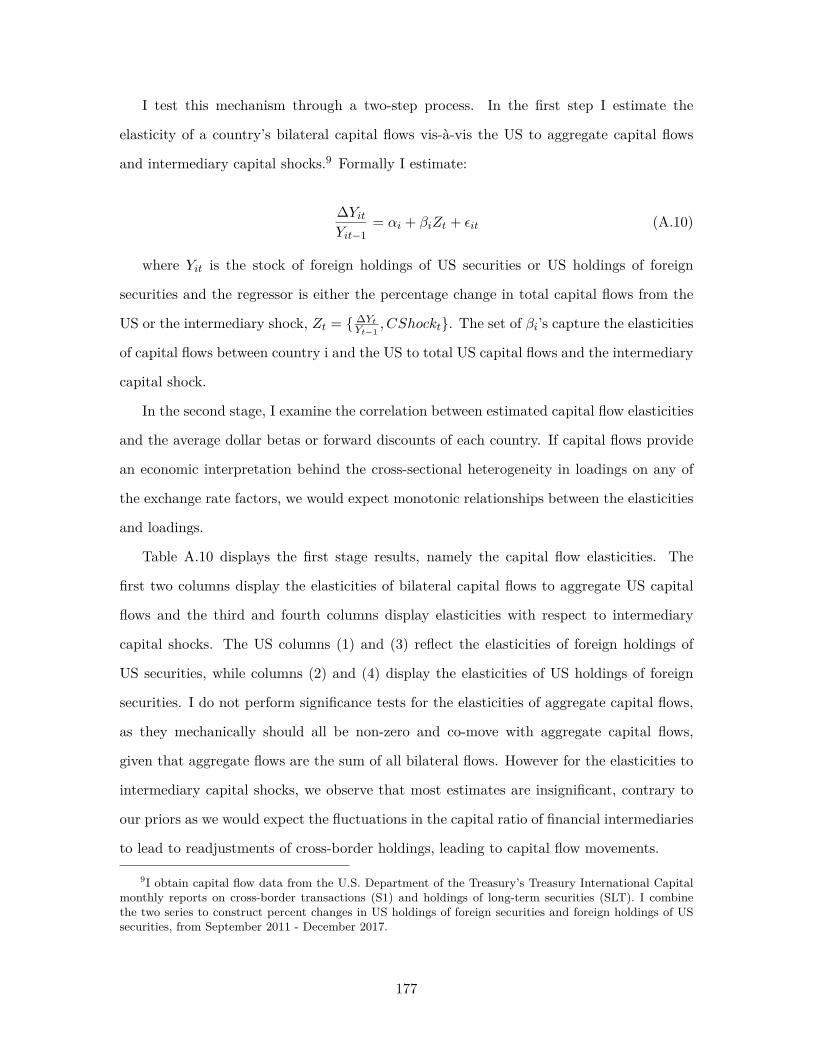
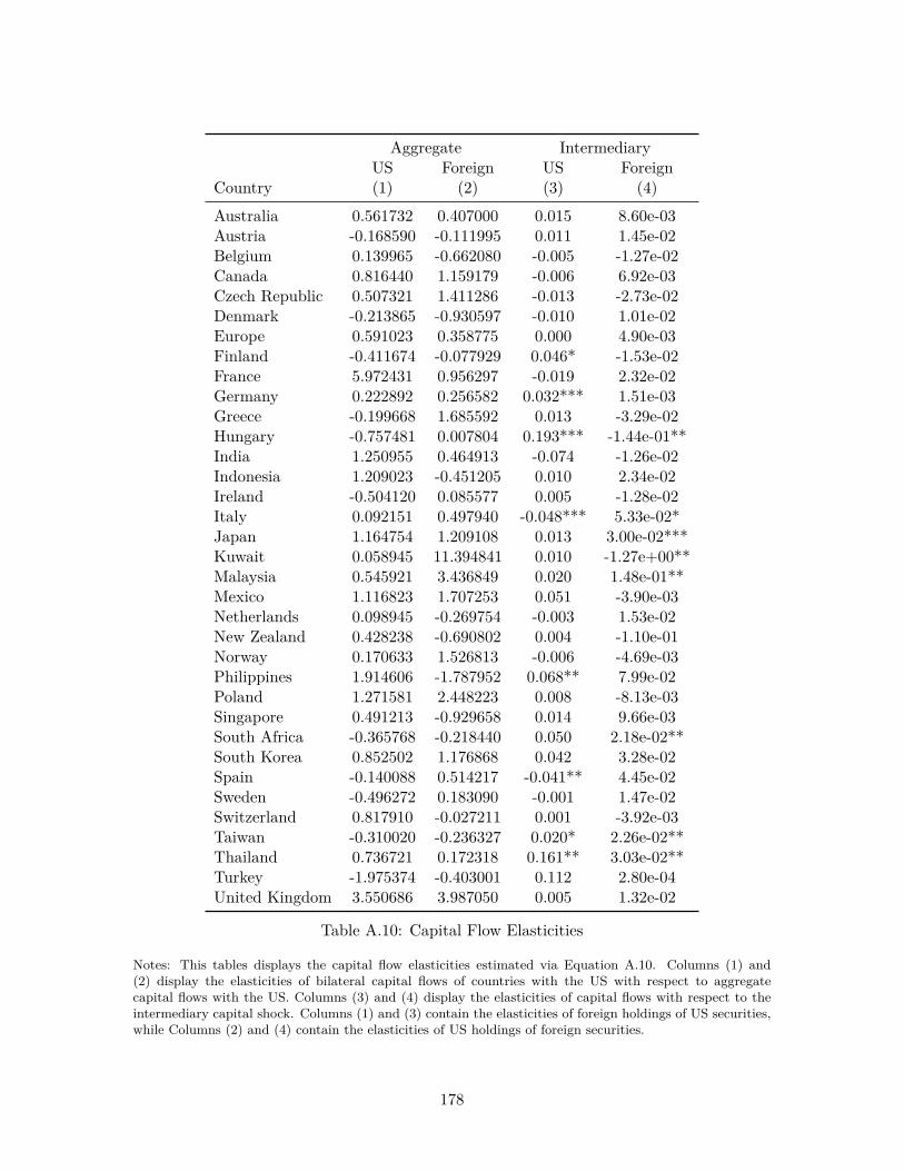
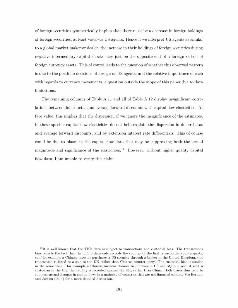
A.11 Correlation Between Capital Flow Elasticities and Dollar Betas . . . . . . . . . 182

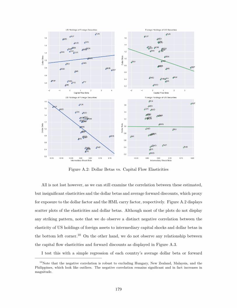
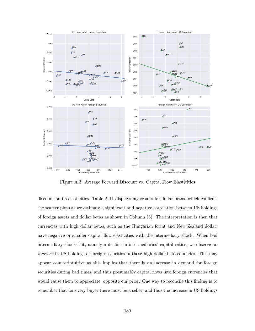
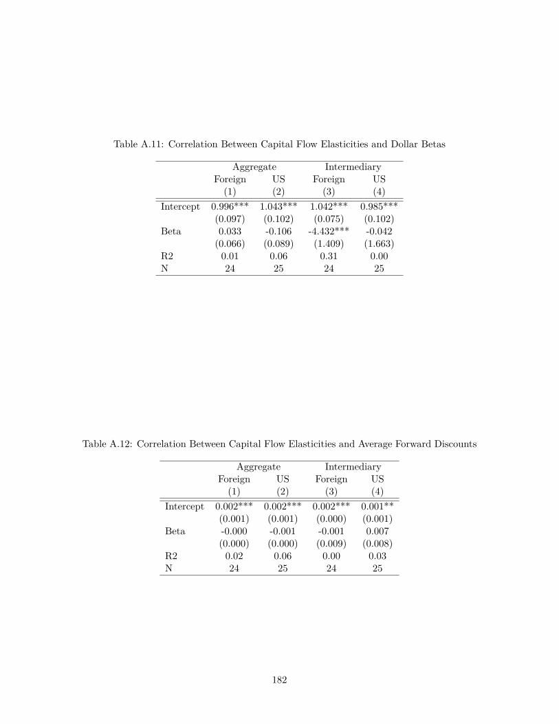
A.12 Correlation Between Capital Flow Elasticities and Average Forward Discounts . 182

vi

Acknowledgements

This dissertation would not have been possible without the guidance and support of my

advisors Richard Clarida, Jennifer La’O, Jón Steinsson, and Jesse Schreger. I owe an

invaluable debt to each of them for taking the time to provide excellent mentorship during

my doctoral studies.

To Rich - I thank you for being the first to get me involved with research, providing

immense guidance and support along the way, and opening doors for me that would not

have been available otherwise. My graduate and future career paths are largely indebted

to you and your role in it was and will always be invaluable.

To Jen-Jen - I cannot thank you enough for your kindness and generosity in taking on

and supporting a young student. You constantly helped and pushed me during my studies

when times were the most difficult, constantly making sure that I was on the right track,

connected to the right individuals, and made opportunities available to me that have helped

shape my career.

To Jón - I thank you for helping me uncover how to critically think about and form

research ideas, questions, and how to approach them in the most effective manner - to

always be a skeptic and constantly strive for a deeper understanding.

To Jesse - I thank you for guiding me through the world of empirical international

vii

finance, taking the time to work closely with me on various topics and projects and help

me navigate the academic world. You taught me how to properly structure an argument

and approach research in a careful and methodological manner, something that I will carry

on well into my career and future.

I also thank various other faculty members that provided useful feedback and support

on my projects: Robert Hodrick, Emi Nakamura, Olivier Darmouni, Matthieu Gomez,

Harrison Hong, Michael Woodford, Patrick Bolton, Martin Uribe, and Stephanie Schmitt-

Grohe. I thank my classmates and other colleagues, especially Cameron LaPoint, Robert

Ainsworth, Michael Connolly, Cynthia Balloch, Falk Gruebelt, Juan Herreno, Chun-Che

Chi, Tyler Abbott, Paolo Cavallino, and Igor Cesarec for useful comments and support

throughout the Ph.D. I thank all participants of the Monetary Economics and Financial

Economics colloquia at Columbia University as well as the Becker Friedman Institute for

providing an opportunity to connect with like-minded scholars and researchers through the

Macro Financial Modeling Project.

Most importantly, I thank my family and friends. You all supported me during this

arduous journey and provided the counsel, reprieve, companionship, and love that made

this dissertation possible. I owe you all the world.

viii

Chapter 1

Intermediary-Based Asset Pricing

and the Cross-Sections of

Exchange Rate Returns

1.1 Introduction

Exchange rates have been a long-standing puzzle for researchers in international macroe-

conomics and finance. Early work by Meese and Rogoff (1983) identified the exchange

rate disconnect, namely the failure of empirical models utilizing monetary and macroeco-

nomic fundamentals as regressors to out-perform a random walk in out-of-sample forecasts

of exchange rates despite the use of ex-post realized values that theory suggests should be

relevant in exchange rate determination. The uncovered interest parity (UIP), one of the

main tenets of international finance that dictates exchange rates must adjust in expectation

to equate returns across countries with differing interest rates, has also failed as Hansen

and Hodrick (1980) and Fama (1984) show that currencies with higher interest rates tend

1

to appreciate rather depreciate, contradicting this basic relationship and giving rise to the

forward premium puzzle and the profitable carry trade strategy. Since the advent of these

studies, scholars have been in search of a cohesive explanation and mechanism to address

these empirical irregularities that contradict the seemingly well-founded theory.

Recent progress has been made on the theoretical front, introducing the notion of fi-

nancial intermediaries and shocks into open economy models that help alleviate some of

the inconsistencies between the models and data (Gabaix and Maggiori 2015, Itskhoki and

Mukhin 2017). At the core of these models is the notion that empirically consistent exchange

rate movements require the presence of constrained agents who intermediate and partici-

pate in foreign exchange markets. Their role as the marginal investors in these markets

causes fluctuations in their risk-bearing capacities to influence exchange rate movements

and consequently serve a central role in exchange rate determination. The risk-based in-

terpretation suggests that if currencies pay off poorly when these intermediaries are more

constrained, precisely when they have lower wealth and highly value an additional unit of

wealth, these currencies are deemed as risky and should provide higher expected returns to

compensate for this downside risk. From a general equilibrium perspective, risky curren-

cies depreciate upon the realization of negative shocks that erode financial intermediaries’

risk-bearing capacity in order to set up a future appreciation that yields higher expected

returns in order to incentivize agents to hold these currencies.

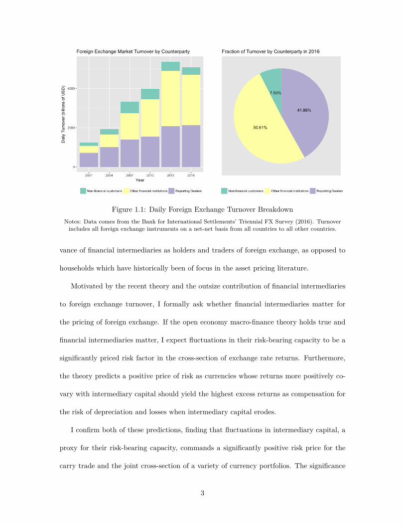
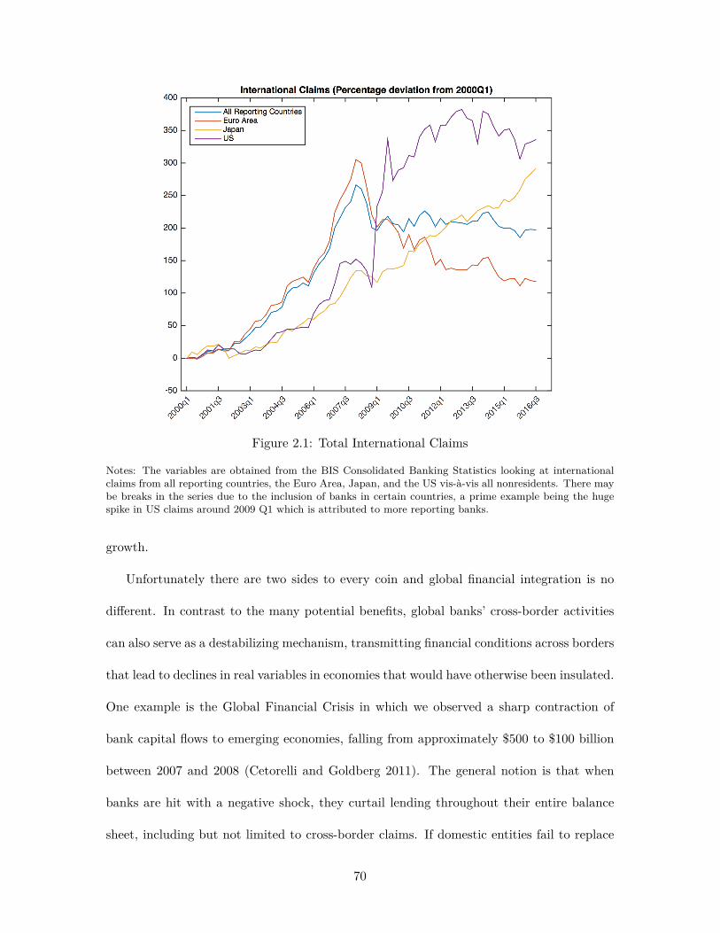
Figure 1.1 displays the composition of foreign exchange volume from the Bank for Inter-

national Settlements Triennial FX survey (2016) over the past decade and a half. The de-

composition shows that an overwhelming portion of exchange rate turnover is attributed to

financial institutions, with the latest survey in 2016 displaying financial institution turnover

of over 90% of the total. The turnover data demonstrates the outsize importance and rele-

2

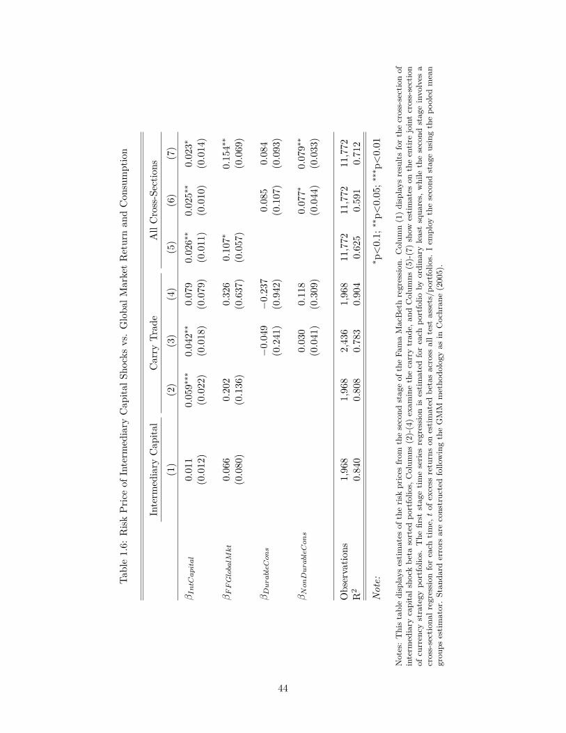
Figure 1.1: Daily Foreign Exchange Turnover BreakdownNotes: Data comes from the Bank for International Settlements’ Triennial FX Survey (2016). Turnoverincludes all foreign exchange instruments on a net-net basis from all countries to all other countries.

vance of financial intermediaries as holders and traders of foreign exchange, as opposed to

households which have historically been of focus in the asset pricing literature.

Motivated by the recent theory and the outsize contribution of financial intermediaries

to foreign exchange turnover, I formally ask whether financial intermediaries matter for

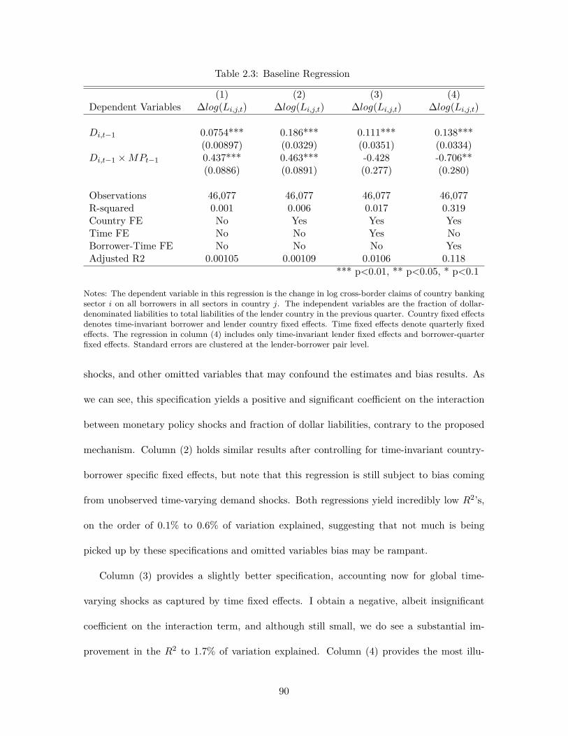
the pricing of foreign exchange. If the open economy macro-finance theory holds true and

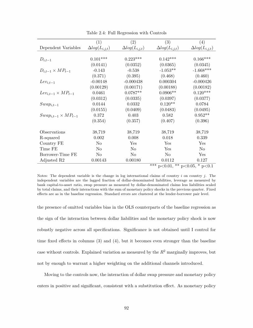
financial intermediaries matter, I expect fluctuations in their risk-bearing capacity to be a

significantly priced risk factor in the cross-section of exchange rate returns. Furthermore,

the theory predicts a positive price of risk as currencies whose returns more positively co-

vary with intermediary capital should yield the highest excess returns as compensation for

the risk of depreciation and losses when intermediary capital erodes.

I confirm both of these predictions, finding that fluctuations in intermediary capital, a

proxy for their risk-bearing capacity, commands a significantly positive risk price for the

carry trade and the joint cross-section of a variety of currency portfolios. The significance

3

of intermediary capital risk for the carry trade indicates that the existence of constrained

intermediaries at the center of foreign exchange markets may provide one explanation for

the failure of the uncovered interest parity as currencies with high interest rates may not

depreciate enough and in fact appreciate due to compensation for the risk of larger depre-

ciations and losses when intermediary capital erodes and agents become more constrained.

The relevance of intermediary capital for the wider joint cross-section suggests that inter-

mediary capital risk underlies a wide range of exchange rate risk premia and thus serves

as a systematic source of global risk. My evidence thus validates open economy models

with a central role for financial intermediaries in foreign exchange markets as I confirm

the risk-based interpretation of exchange rate risk premia through the lens of financial

intermediaries.

Following my confirmation of intermediary-based asset pricing models for exchange

rates, I assess their performance in comparison to a traditional consumption-based asset

pricing model. This exercise serves to elucidate whether financial intermediaries or house-

holds are the most relevant marginal investors, revealing whether models actually require

financial intermediaries. I find that intermediary capital risk remains significant for both

the carry trade and joint cross-section upon inclusion of consumption growth, consistent

with intermediary-based asset pricing as it is intermediary capital risk rather than house-

hold consumption risk that prices foreign exchange, in line with intermediaries’ roles as the

marginal investors.

I also compare fluctuations in intermediary capital to previously identified exchange

rate factors, namely the high-minus-low (HML) carry and dollar and global dollar factors

of Lustig, Roussanov, and Verdelhan (2011, 2014) and Verdelhan (2018), in order to deter-

mine whether the risk-bearing capacity of financial intermediaries serves as one economic

4

explanation for the risk contained within these factors. While factors constructed through

portfolio-based methods provide an appealing proxy for underlying and generally unobserv-

able risk factors, the economic sources of these risks are not clearly identified. I seek to

fill this void by delineating whether intermediary capital serves as an independent source

or one of the many sources of risk contained within these factors, shedding light upon the

economic content of the HML carry and global dollar factors. I find that the HML carry

factor serves as the most robust pricing factor for exchange rates, subsuming the previously

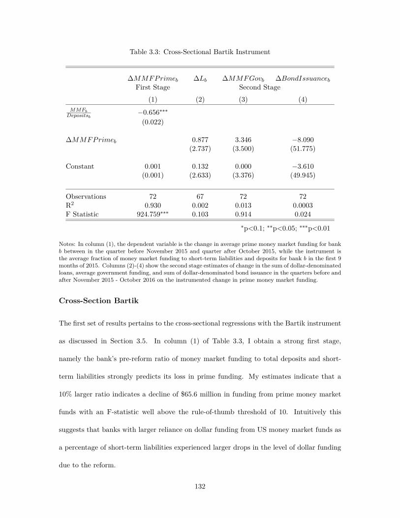
significant intermediary capital risk, thus providing evidence that intermediary capital risk

serves as a sub-component of the HML carry factor which contains a wider set of economic

shocks and risk. Intermediary capital appears to be an independent and more relevant

source of exchange rate risk compared to the dollar and global dollar factors, but interme-

diary capital does positively co-vary with the latter factor, suggestive that some of the risk

contained within the global dollar factor is related to the risk-bearing capacity of financial

intermediaries.

Taking a step back, recall that in standard asset pricing theory the value of an asset

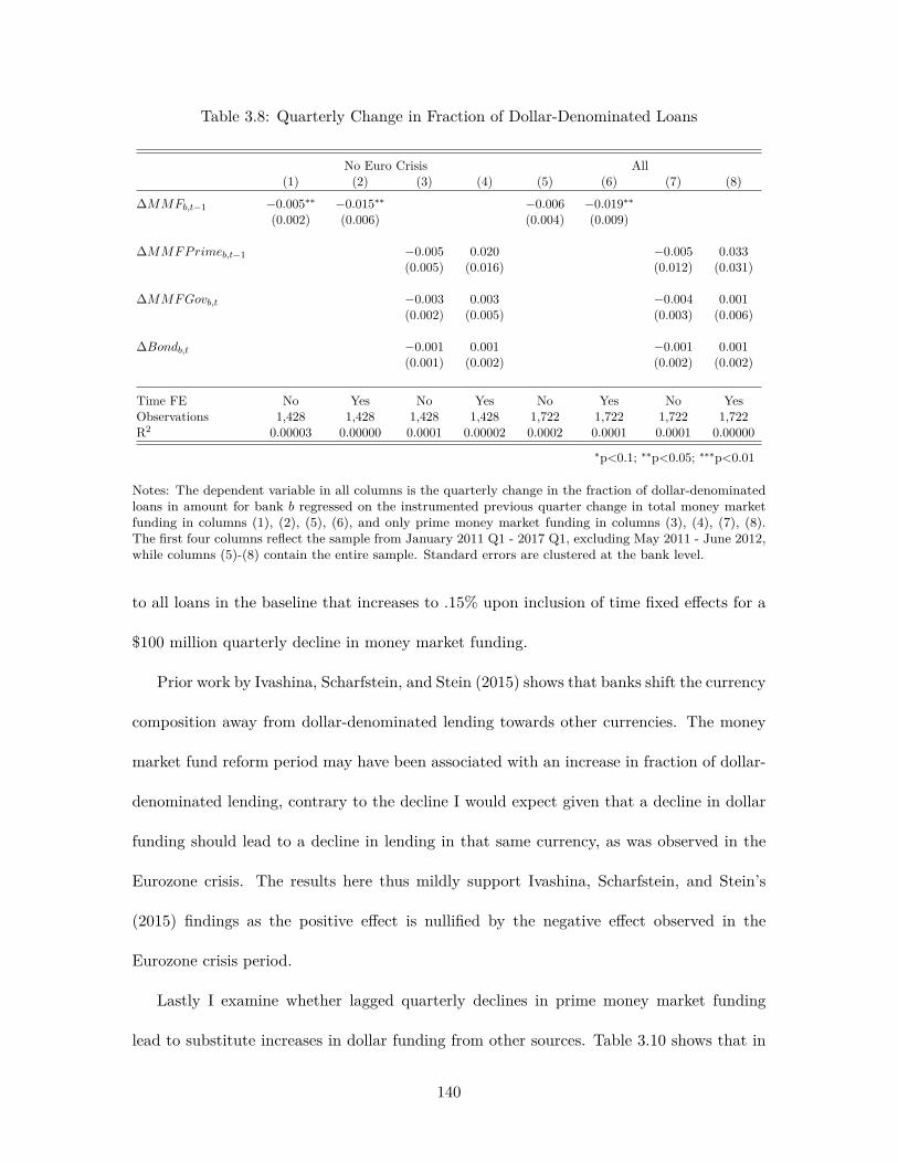
is determined by the marginal investor’s trade-off between current and future consumption

in combination with the asset’s prospective cash-flows, where the marginal investor is the

agent holding the asset. The relative value of consumption is given by the marginal utility

or pricing kernel of this agent and thus asset prices and expected returns should jointly

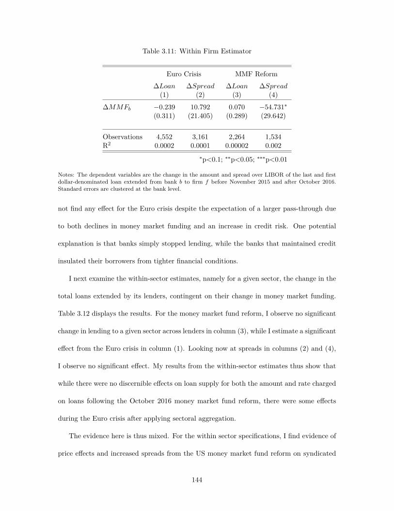
fluctuate with her marginal utility. Assets that provide poor returns when the marginal

investor encounters low consumption, and equivalently high marginal utility, should provide

higher expected returns as otherwise the agent would have no incentive to hold this riskier

asset. Traditional asset pricing models have focused on households as the marginal investors,

a by-product of representative agent models where households are the sole bearers of assets,

5

and have investigated the relevance of measures of households’ marginal utility such as

consumption growth to test this theory. These models however have generally failed and/or

entertain implausible coefficients for risk aversion (Mehra and Prescott 1985, Lustig and

Verdelhan 2007).

The outsize importance of financial intermediaries in the trading and holding of financial

assets motivates a shift towards the analysis of the marginal utilities and pricing kernels of

these more relevant agents in both theory and empirics, suggesting that we must focus on

their presumably central role in asset pricing instead of that of households. The recently

well-developed closed-economy macro-finance literature has shown that models with real-

istic, time-varying risk premia (Brunnermeier and Sannikov 2014, He and Krishnamurthy

2013, Garleanu and Pedersen 2011) hinge on the presence of constrained financial interme-

diaries as the marginal investors. The level of constraint of these intermediaries, whether

through a measure of their leverage, equity capital ratio, or margin requirements, thus en-

ters as a state variable and determinant of their marginal utility and assets are then priced

via the following mechanism: when intermediaries are more constrained, their marginal

utilities are high as they would prefer higher consumption or wealth but are unable to

borrow or lever up due to their constraint. It is then the covariance of asset returns with

these determinants of marginal utility that dictates the size and presence of risk premia as

assets that provide poor returns during periods of high constraints and consequently high

marginal utility must yield larger expected returns to compensate for this downside risk.

This intuition can be extended to foreign exchange markets. When the marginal utility

of intermediaries is high, perhaps due to negative shocks that lower their net worth and

constrain their ability to trade or absorb losses, currencies that depreciate are considered

risky assets as they lose value during bad times and should provide higher expected returns

6

to compensate. Similarly, currencies that appreciate when intermediaries are more con-

strained should provide lower expected returns as they serve as insurance or hedges in the

face of adverse shocks. This risk-based interpretation of exchange rate returns motivates

the recent portfolio-based studies of exchange rates and the approach of this paper.

I confirm the validity of this mechanism by looking at the relevance of fluctuations in

the capital ratios of financial intermediaries, examining whether these financial shocks are

priced into the cross-section of exchange rate returns across portfolios of various strategies

above and beyond other economic factors, namely consumption growth and the broader

market return, and currency-specific factors such as the HML carry, dollar, and global

dollar factors. I construct and employ currency portfolios to mitigate the influence of

idiosyncratic country-specific risk and more accurately estimate betas while also assessing

whether the risk premia captured by a wide range of cross-sections of currencies may be

rationalized by the central role of financial intermediaries, a potential economic source of

systematic global risk. While the recent literature has mainly focused on the identification

of novel cross-sections of returns and sources of common variation across exchange rates

through portfolio-based methods, little has been said about the fundamental economic

determinants of the sources of risk that drive the heterogeneity in currency returns. I

delineate the relevance of fluctuations in intermediary capital as an economic source of risk

embedded in the various cross-sections of foreign exchange returns and assess whether it is

distinct from or merely a component of the previously identified risk factors that do not

yet have definitive economic interpretations.

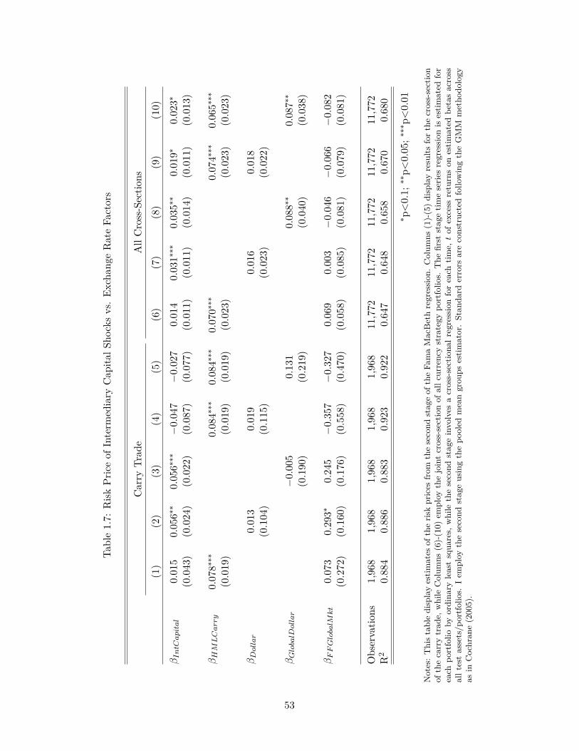
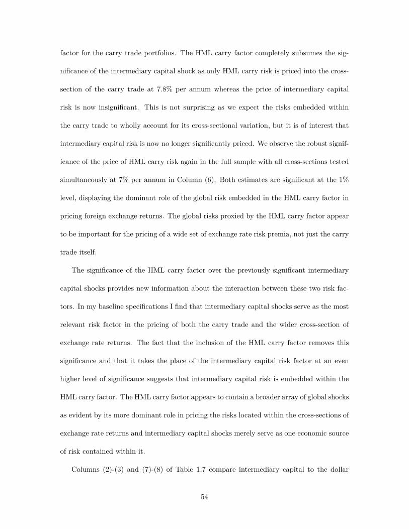
As alluded to before, I find that intermediary capital is a significant risk factor for the

pricing of the carry trade and joint cross-section of foreign exchange portfolio returns when

compared to consumption growth and the broader equity market. Currencies that more

7

positively co-vary with fluctuations in intermediary capital, or high intermediary capital

beta currencies, provide higher excess returns and vice-versa, in line with intuition and

providing support for the relevance of the risk-bearing capacity of financial intermediaries

as an economic source of risk for exchange rates. My results confirm the validity of this

mechanism as I show that intermediary capital commands a significant and positive risk

price when examining the carry trade in isolation and the joint cross-section of currency

portfolios covering a diverse set of risk premia. My findings show that financial intermedi-

aries provide one explanation for the forward premium puzzle and failure of the uncovered

interest parity, rationalizing the higher excess returns captured by high interest rate curren-

cies through a risk-based interpretation of exchange rate movements, while also identifying

intermediary capital as a source of global risk that underlies a broad set exchange rate risk

premia.

I also show that while intermediary capital risk serves as a significant risk factor relative

to other proposed economic risk factors, it is subsumed by the portfolio-generated HML

carry factor as intermediary capital risk is no longer or only marginally significant upon the

inclusion of the robustly priced HML carry risk factor. This finding does not preclude the

relevance of intermediary capital risk and in fact clarifies its role in relation to previously

identified sources of global risk embedded in the cross-section of exchange rates. The

fact that the price of intermediary capital risk is previously significant and subsequently

overshadowed by the HML carry risk factor shows that it may be one source of risk contained

within the latter factor. Previous studies have shown the relevance of the HML carry risk

factor, but have not yet conclusively identified its economic determinants with respect to

financial shocks. The results here suggest that HML carry is the dominant risk factor

for exchange rates and that intermediary capital shocks are one economic source of risk

8

embedded within it.

In addition to the findings on the interplay of intermediary capital risk with the HML

carry risk factor, I also provide an analysis of its connection with the dollar and global

dollar factors of Lustig, Roussanov, and Verdelhan (2011) and Verdelhan (2018). I find

that intermediary capital risk maintains its relevance when compared to these two factors

and that the relevance of the risk embedded in the dollar factors for the cross-section of

exchange rates hinges on the isolation of the global risk obtained by parsing out the US-

specific component of risk - the global dollar factor is significantly priced in the wider

cross-section of currency returns whereas the dollar factor itself is not.

I proceed to formally examine whether intermediary capital shocks explain some compo-

nent of the HML carry and global dollar factors given that I hypothesize that intermediary

capital risk serves an one economic source of shocks embedded in these two factors, while

also exploring the relevance of other candidate sources of global risk. I find that interme-

diary capital is a robust source of risk contained within the HML carry factor, consistent

with the economic relevance of intermediary risk for the pricing of foreign exchange. I also

document the relevance of other economic sources of risk, namely risk aversion, liquidity,

and US real activity for the HML carry factor, in line with previous studies and theory,

and the co-movement of intermediary capital, liquidity, and US real activity for the global

dollar factor, shedding light upon potential economic sources of risk contained within this

less studied factor.

The paper proceeds as follows. Section 1.2 discusses where this paper lies in the broader

literature. Section 1.3 describes the core data, portfolio construction methodology, and

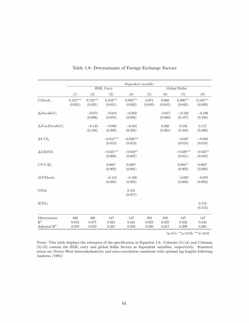
various summary statistics. Section 1.4 outlines the regression specifications, and displays

and discusses the empirical asset pricing results. Section 1.5 examines the economic deter-

9

minants of the portfolio-based exchange rate factors. Section 1.6 concludes.

1.2 Literature Review

This paper relates to a few strands of literature, most notably that on intermediary-based

asset pricing and the portfolio, risk-based studies of exchange rates. More broadly it leans

on the intuition from closed economy macro-finance models and seeks to validate recent

open economy general equilibrium models that include financial intermediaries and shocks.

The notion of intermediary-based asset pricing has been identified and tested by previous

researchers, but a deeper examination of its relevance for exchange rates has not. Adrian,

Etula, and Muir (2014) were the first to empirically test for the relevance of intermediaries

in asset pricing, using the leverage of the US broker dealer sector as a proxy for the marginal

value of wealth of financial intermediaries to find significant prices of intermediary risk for

the excess returns of various portfolios of US equities and bonds, and out-performance in

a variety of other metrics, above and beyond that of mainstream asset pricing models.

He, Kelly, and Manela (2017) perform a more expansive assessment, constructing their

proxy for the marginal value of wealth of intermediaries via the net worth, or capital

ratio, of primary dealers with the New York Fed, and test their factor on stocks, bonds,

credit default swaps, exchange rates, and commodities, finding a significant risk price of

intermediary capital. It is important to note that these two seminal papers have conflicting

findings as Adrian, Etula, and Muir (2014) find evidence for pro-cyclical leverage and a

positive price of intermediary leverage risk, whereas He, Kelly, and Manela (2017) find

evidence for counter-cyclical leverage and a positive price of intermediary capital risk. These

findings are contradictory as leverage should simply be the inverse of the capital ratio

and thus the prices of risk should be inverted as well. While macro-finance models can

10

generate both results depending on whether the intermediary has a debt or equity constraint

respectively, I follow He, Kelly, and Manela (2017) as their measure of intermediary shocks is

available at the monthly level in contrast to the quarterly frequency of the leverage measure

from Adrian, Etula, and Muir (2014). My paper departs from both by shifting focus to

the foreign exchange market, employing a wider set of exchange rate cross-sections, and

studying the relevance and interplay of intermediary shocks against previously established

risk factors in the empirical foreign exchange asset pricing literature in search of an economic

interpretation for the global shocks that drive foreign exchange returns.

Related to the connection between financial shocks and exchange rates, Adrian, Etula,

and Shin (2015) show that measures of short-term US dollar funding, namely primary

dealer repos and commercial paper outstanding, forecast appreciations of the dollar and

estimate a dynamic asset pricing model following Adrian, Crump, and Moench (2015) to

find significant prices of carry and short-term dollar funding risk for the entire cross-section

of individual currency excess returns. I deviate from their work by focusing the relationship

between the carry trade and intermediary capital to uncover whether intermediary capital

prices the carry trade and thus helps explains the forward premium puzzle, and the joint

cross-section of currency portfolios to identify the existence of a systematic global risk factor

with a meaningful economic interpretation. I also link the intermediary shocks back to their

relationship with the HML carry and global dollar factors.

The empirical international finance literature on exchange rates has shifted towards

portfolio-based tests of risk premia and the identification of novel cross-sections of currency

excess returns. This was first applied by Lustig and Verdelhan (2007) who form portfolios of

currencies based on their interest rate differentials and find significant prices of consumption

risk in the cross-section of exchange rate returns, arguing that exposure to US consumption

11

risk explains the carry trade and the forward premium puzzle. Lustig, Roussanov, and

Verdelhan (2011) continue this approach and find that the cross-section of carry trade

returns is driven by two factors, namely a level and slope factor. They show that sorting

currencies by their forward discounts as a proxy for interest rate differentials leads to a

monotonic relationship in excess returns by portfolio and identify the high-minus-low (HML)

carry factor that is significantly priced in the cross-section and highly correlated with the

currency slope factor. In addition, they find that the level factor is highly correlated with the

average excess returns of foreign currencies against the dollar and establish this level factor

as the dollar factor. Building on Backus, Foresi, and Telmer (2001), they interpret their

findings through the lens of an affine model of exchange rates that identifies the necessity

of heterogeneous loadings on a global factor that can be proxied by the HML carry factor

in order to theoretically generate the cross-section of carry trade returns.

The level or dollar factor is explored in subsequent papers, namely Lustig, Roussanov,

and Verdelhan (2014) and Verdelhan (2018). These papers identify cross-sections of cur-

rency returns distinct from the carry trade hinged on going long foreign currencies and short

the US dollar when the average forward discount is positive, with the risk of depreciation

of foreign currencies when bad shocks hit in times with high US volatility and thus high

US investor marginal utility. This paper can rationalize this mechanism as US investor

marginal utility may be proxied by the risk-bearing capacity of financial intermediaries if

they are indeed the marginal investors in currency markets. Verdelhan (2018) highlights

the share of systematic variation in bilateral exchange rates, noting the outsize importance

of the average change in the US dollar against all foreign currencies, or what he calls the

dollar factor, in the explained variation of exchange rate movements. He identifies a sepa-

rate cross-section based on heterogeneous movements relative to this dollar factor, namely

12

the dollar betas, and establishes the notion of a global dollar factor by taking the difference

between high and low dollar beta sorted portfolios to isolate the global risk factor driving

this separate cross-section that is purged of US-specific risk. He then finds that this cross-

section of dollar portfolios is distinct from the carry trade and rationalizes its existence by

positing an affine model with two orthogonal global shocks to generate both cross-sections,

each of which can be proxied by the HML carry and global dollar factors. My paper seeks

to shed light upon the economic content of these factor in relation to intermediary-based

asset pricing.

I borrow from and build upon this line of papers by forming portfolios of currencies

as test assets sorted by forward discounts as in Lustig, Roussanov, and Verdelhan (2011),

dollar betas as in Verdelhan (2018), and a variety of other cross-sections previously identified

in the literature (Asness, Moskowitz, and Pedersen (2013), Menkhoff et al. 2012a, 2012b),

and utilize the identified risk factors, namely the HML carry, dollar, and global dollar

factors to compare to the intermediary capital shocks. I employ portfolios to reduce the

influence of idiosyncratic, country-specific risk and combine portfolios from this diverse set

of cross-sections to assess whether financial intermediaries serve as a source of systematic

global risk that is present in exchange rate risk premia. My goal is similar to this line

of research as I attempt to find another cross-section of currency returns and risk, but

also complement it by examining the interplay between the intermediary shocks, previously

identified exchange rate factors, and various cross-sections of currency portfolio returns.

More importantly, given the portfolio-based approach of identifying risk factors, previous

papers do not explicitly identify the economic source of the shocks contained within the

HML carry and global dollar risk factors or an explanation of the heterogeneous loadings

on these shocks in the lens of affine exchange rate models, although Lustig, Roussanov, and

13

Verdelhan (2011) and Verdelhan (2018) do draw some connections between equity market

volatility and the HML carry factor, and systematic exposure to global capital flows and

the global dollar factor, respectively.

There also exists an immense literature on the carry trade and this paper contributes

by highlighting that fluctuations in intermediary capital serve as one economic explanation

behind its existence. Lustig and Verdelhan (2007) find the significance of US consumption

growth, borrowing from Yogo’s (2006) D-CAPM model to show that currency portfolios

sorted on interest rate differentials align with consumption betas, providing evidence in

support of consumption-based asset pricing as applied to foreign exchange. Burnside (2011)

debates their findings on the basis of econometric issues, arguing that after accounting for

the estimated regressors problem associated with the first-stage consumption betas and

properly adjusting standard errors, he finds no significant risk price of consumption growth.

My work builds upon both by comparing the relevance of intermediary capital to that of

consumption growth, constructing standard errors that correct for the estimated first stage

betas, and clarifying whether it is intermediaries or households that price the carry trade and

broader cross-section of exchange rate returns. This exercise serves to distinguish between

traditional consumption- and intermediary-based asset pricing models and validate whether

the introduction of financial intermediaries into open economy models is warranted.

A series of papers examines the relevance of crash risk and peso problems to account for

the carry trade. Brunnermeier, Nagel, and Pedersen (2008) identify the negative skewness

of the carry trade, revealing the presence of infrequent, but large carry trade draw-downs

and show that increases in global risk aversion coincide with carry trade losses. Burnside

et al. (2011) argue for the relevance of peso problems as they find that traditional risk

factors fail to price the carry trade, while the hedged carry trade provides lower returns

14

compared to the traditional un-hedged version, indicative of compensation for downside

risk. They proceed to show that the peso problem stems from high values of the marginal

investor’s stochastic discount factor in the peso state rather than large losses. Jurek (2014)

provides a similar analysis and constructs a crash-neutral carry trade by hedging with out-

of-the-money options, but he comes to a different conclusion. He shows that although

the hedged carry trade provides slightly lower returns compared to the un-hedged version,

there still exist significant excess returns to both and compensation for a peso state can

only account for one-third of carry trade returns, which he interprets as an inability of peso

problems to fully account for the existence of the carry trade. Lettau, Maggiori, and Weber

(2014) document the downside-CAPM model that significantly prices the carry trade and

a wide variety of assets, arguing for the asymmetry between risk premia associated with

market declines and increases. Farhi and Gabaix (2016) introduce rare disaster risk into

an open economy model, suggesting that some countries have higher interest rates because

their currencies disproportionately depreciate when disasters arrive and investors must be

compensated for this disaster risk through positive expected returns.

This paper connects to this literature by showing that financial intermediaries’ risk-

bearing capacity can be one way to rationalize crash risk. Burnside et al.’s (2011) finding

that marginal utilities are disproportionately high in peso states for which the carry trade

is compensated for is consistent with intermediary-based asset pricing as in times when

intermediary capital is low and they are constrained, their marginal utility of wealth and

thus stochastic discount factor is high, with risk premia sharply rising when intermediaries

are almost or fully constrained. One class of peso event can then be financial crises in which

intermediaries are constrained and demand higher risk premia, consistent with the closed-

economy intermediary-based asset pricing literature. Similarly, down-side and disaster risk

15

can be viewed through the lens of intermediary-based asset pricing as currencies that more

positively load onto intermediary capital risk should disproportionately depreciate upon

realizations of large negative capital shocks that lead intermediaries to become increasingly

or completely constrained.1 Furthermore, the relevance of global risk-aversion can also

be interpreted through intermediary-based asset pricing as intermediaries with lower risk-

bearing capacities should endogenously become more risk averse, thus commanding higher

risk-premia and I confirm Brunnermeier, Nagel, and Pedersen’s (2008) finding that risk

aversion is negatively associated with carry trade returns.

Menkhoff et al. (2012), Hassan (2013), Daniel, Hodrick, and Lu (2017), Ready, Rous-

sanov, and Ward (2017), Richmond (2016), and Jiang (2018) provide a variety of alternate

explanations for the cross-section of carry trade returns due to volatility risk, country size,

dollar and equity risk, commodity exporters, trade networks, and fiscal risks, respectively,

and I look to add to this literature by examining whether intermediary capital risk can

also provide an economic explanation of the carry trade. I go beyond these papers by

assessing whether intermediary capital accounts for not only the carry trade, but also the

joint cross-section of a variety of currency portfolios, showing that intermediary-based as-

set pricing alone provides an elegant and fundamental economic explanation to the forward

premium puzzle and reveals an economic risk factor that underlies a wide set of exchange

rate risk premia. In addition, the economic interpretations behind the shocks contained in

the dollar and global dollar factors identified by Lustig, Roussanov, and Verdelhan (2011)

and Verdelhan (2018) are less widely studied and I approach both through the lens of finan-

cial intermediaries, and a provide a formal analysis of potential determinants of the global

1This paper does not explicitly account for non-linearities in the asset pricing tests. Non-linearities arehowever explicitly modeled in the closed economy macro-finance literature, e.g. He and Krishnamurthy(2013) and Brunnermeier and Sannikov (2014).

16

dollar factor.2

The empirical intermediary-based asset pricing literature is based predictions from the

closed economy macro-finance literature that hinges upon the existence of constrained fi-

nancial intermediaries. Brunnermeier and Sannikov (2014), He and Krishnamurthy (2013),

Danielsson, Shin, and Zigrand (2011), Adrian and Boyarchenko (2012), Garleanu and Ped-

ersen (2011), Brunnermeier and Pedersen (2009) explore macro-finance models with con-

strained intermediaries whose relative risk-bearing capacities, net worth, and/or leverage

matter for the behavior of risk premia and thus asset prices. Most closely related to this

paper is He and Krishnamurthy (2013) who construct a model in which financial inter-

mediaries serve as the marginal investors in risky assets as households are restricted from

holding these assets and can only gain exposure by funding intermediaries who invest on

their behalf. Intermediary net worth, and equivalently risk-bearing capacity, plays a central

role as households only invest up to a fraction of the intermediary’s net worth, which can

be interpreted as providing an incentive for intermediaries to optimally choose their port-

folios as poor choices will negatively erode their capital and dry up their funding, leaving

them more constrained. Non-linearities arise in the model because when the intermediary

becomes fully constrained, risk premia sharply rise, in contrast to the unconstrained region.

The notion of financial intermediaries in macroeconomic models has also been extended

to the open economy. Gabaix and Maggiori (2015) develop an open economy model with a

constrained global financier/bank that intermediates all international bond trades and show

that their model produces intuitive exchange rate movements that emphasize the role of the

risk-bearing capacity of financial intermediaries and portfolio flows in exchange rate deter-

2In Appendix A.3 I explore whether capital flow elasticities to fluctuations in intermediary capital alignwith the dollar betas, finding a positive relationship between the two. My results point towards capital flowsin relation to intermediary capital as an economic rationale behind the pattern of dollar betas.

17

mination. Their paper also contains theoretical predictions regarding the carry trade and

the risk-bearing capacity of financial intermediaries as they show that carry trade returns

erode upon realizations of shocks that negatively impact the intermediary’s risk-bearing ca-

pacity and that intermediaries must be compensated for holding currencies that depreciate

upon the realization of tighter financial conditions - I confirm their theoretical predictions in

both asset pricing and standard regression tests. Itskhoki and Mukhin (2017) emphasize the

role of financial shocks in general equilibrium open economy models, namely through a UIP

wedge, to produce empirically consistent exchange rate movements. The financial shocks in

their model can be interpreted as fluctuations in the risk-bearing capacity of financial inter-

mediaries that drive deviations from the UIP as more constrained intermediaries will be less

inclined to remove and balance deviations in the UIP and must be compensated via higher

expected returns to hold high interest rate currencies that run the risk of depreciation. This

paper thus seeks to validate the role of financial intermediaries for consistent exchange rate

behavior by measuring whether risks emanating from their existence can account for the

cross-sectional heterogeneity in excess returns across currencies and the predictions of the

models are borne out in the data. I however abstract from writing down a full structural

open economy model with constrained financial intermediaries, leaving that open to future

research.

1.3 Data

Currencies

I obtain daily spot and forward data from Datastream, combining Barclays and

WM/Reuters data as the former extends farther back but with less currencies, whereas

18

the latter contains the full set of currencies. To remain consistent with previous studies, I

splice the datasets in January 1997, using the Barclays data prior to this date and only the

WM/Reuters data after. I obtain an end-of-the-month series for each currency from Jan-

uary 1983 to March 2018 subject to availability. All spot and forward rates are expressed

in US dollars, or quoted as foreign currency units per dollar. The dataset covers the fol-

lowing countries: Australia, Austria, Belgium, Canada, Czech Republic, Denmark, Euro

area, Finland, France, Germany, Greece, Hong Kong, Hungary, India, Indonesia, Ireland,

Italy, Japan, Kuwait, Malaysia, Mexico, Netherlands, New Zealand, Norway Philippines,

Poland, Portugal, Saudi Arabia, Singapore, South Africa, South Korea, Spain, Sweden,

Switzerland, Taiwan, Thailand, Turkey, the United Arab Emirates, and the United King-

dom. Countries that adopted the euro are kept until January 1999, and I contrast with the

existing literature by omitting the pegged currencies of Hong Kong, Saudi Arabia, and the

United Arab Emirates.

To remain consistent with the previous literature, I delete the following observations

as in Lustig, Roussanov, and Verdelhan (2011) and corresponding papers due to large

failures of covered interest parity: South Africa from July 1985 to August 1985, Malaysia

from August 1998 to June 2005, Indonesia from December 2005 to May 2007, Turkey from

October 2000 to November 2001, and United Arab Emirates from June 2006 to November

2006. Note that since the financial crisis there have been widespread deviations in covered

interest parity (Du, Tepper, Verdelhan 2018), but I abstain from deleting observations in

the latter part of the sample given the prevalence of deviations for most developed countries.

19

Intermediary Capital Shocks

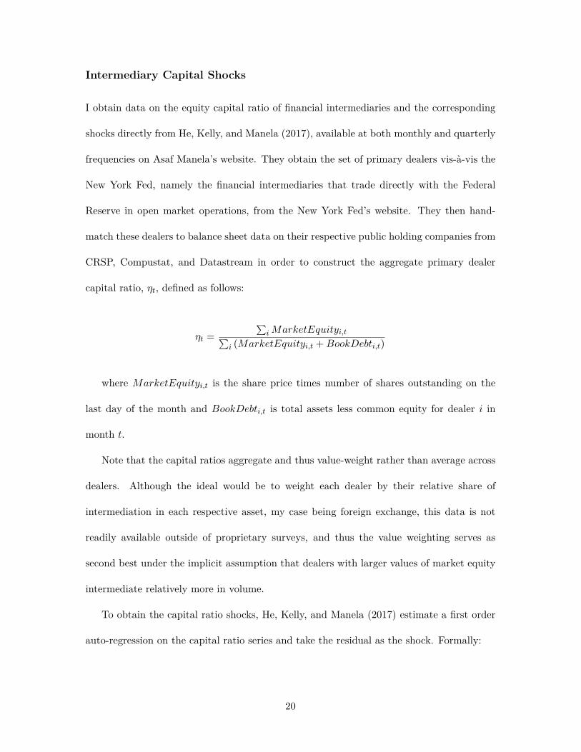
I obtain data on the equity capital ratio of financial intermediaries and the corresponding

shocks directly from He, Kelly, and Manela (2017), available at both monthly and quarterly

frequencies on Asaf Manela’s website. They obtain the set of primary dealers vis-à-vis the

New York Fed, namely the financial intermediaries that trade directly with the Federal

Reserve in open market operations, from the New York Fed’s website. They then hand-

match these dealers to balance sheet data on their respective public holding companies from

CRSP, Compustat, and Datastream in order to construct the aggregate primary dealer

capital ratio, ηt, defined as follows:

ηt =

∑iMarketEquityi,t∑

i (MarketEquityi,t +BookDebti,t)

where MarketEquityi,t is the share price times number of shares outstanding on the

last day of the month and BookDebti,t is total assets less common equity for dealer i in

month t.

Note that the capital ratios aggregate and thus value-weight rather than average across

dealers. Although the ideal would be to weight each dealer by their relative share of

intermediation in each respective asset, my case being foreign exchange, this data is not

readily available outside of proprietary surveys, and thus the value weighting serves as

second best under the implicit assumption that dealers with larger values of market equity

intermediate relatively more in volume.

To obtain the capital ratio shocks, He, Kelly, and Manela (2017) estimate a first order

auto-regression on the capital ratio series and take the residual as the shock. Formally:

20

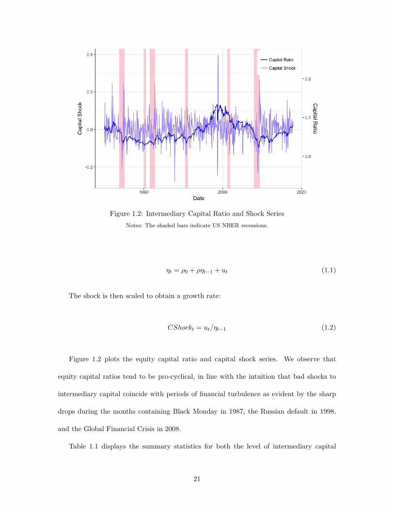
Figure 1.2: Intermediary Capital Ratio and Shock SeriesNotes: The shaded bars indicate US NBER recessions.

ηt = ρ0 + ρηt−1 + ut (1.1)

The shock is then scaled to obtain a growth rate:

CShockt = ut/ηt−1 (1.2)

Figure 1.2 plots the equity capital ratio and capital shock series. We observe that

equity capital ratios tend to be pro-cyclical, in line with the intuition that bad shocks to

intermediary capital coincide with periods of financial turbulence as evident by the sharp

drops during the months containing Black Monday in 1987, the Russian default in 1998,

and the Global Financial Crisis in 2008.

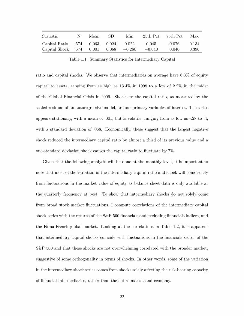
Table 1.1 displays the summary statistics for both the level of intermediary capital

21

Statistic N Mean SD Min 25th Pct 75th Pct MaxCapital Ratio 574 0.063 0.024 0.022 0.045 0.076 0.134Capital Shock 574 0.001 0.068 −0.280 −0.040 0.040 0.396

Table 1.1: Summary Statistics for Intermediary Capital

ratio and capital shocks. We observe that intermediaries on average have 6.3% of equity

capital to assets, ranging from as high as 13.4% in 1998 to a low of 2.2% in the midst

of the Global Financial Crisis in 2009. Shocks to the capital ratio, as measured by the

scaled residual of an autoregressive model, are our primary variables of interest. The series

appears stationary, with a mean of .001, but is volatile, ranging from as low as -.28 to .4,

with a standard deviation of .068. Economically, these suggest that the largest negative

shock reduced the intermediary capital ratio by almost a third of its previous value and a

one-standard deviation shock causes the capital ratio to fluctuate by 7%.

Given that the following analysis will be done at the monthly level, it is important to

note that most of the variation in the intermediary capital ratio and shock will come solely

from fluctuations in the market value of equity as balance sheet data is only available at

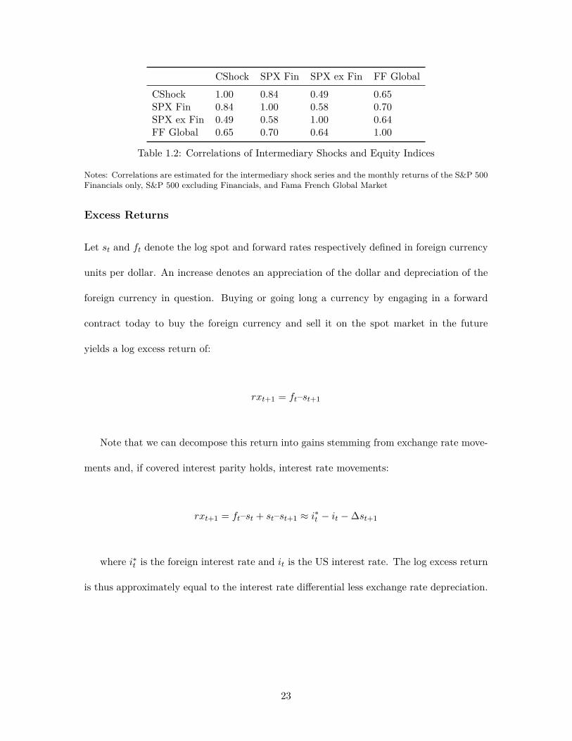
the quarterly frequency at best. To show that intermediary shocks do not solely come

from broad stock market fluctuations, I compute correlations of the intermediary capital

shock series with the returns of the S&P 500 financials and excluding financials indices, and

the Fama-French global market. Looking at the correlations in Table 1.2, it is apparent

that intermediary capital shocks coincide with fluctuations in the financials sector of the

S&P 500 and that these shocks are not overwhelming correlated with the broader market,

suggestive of some orthogonality in terms of shocks. In other words, some of the variation

in the intermediary shock series comes from shocks solely affecting the risk-bearing capacity

of financial intermediaries, rather than the entire market and economy.

22

CShock SPX Fin SPX ex Fin FF GlobalCShock 1.00 0.84 0.49 0.65SPX Fin 0.84 1.00 0.58 0.70SPX ex Fin 0.49 0.58 1.00 0.64FF Global 0.65 0.70 0.64 1.00

Table 1.2: Correlations of Intermediary Shocks and Equity Indices

Notes: Correlations are estimated for the intermediary shock series and the monthly returns of the S&P 500Financials only, S&P 500 excluding Financials, and Fama French Global Market

Excess Returns

Let st and ft denote the log spot and forward rates respectively defined in foreign currency

units per dollar. An increase denotes an appreciation of the dollar and depreciation of the

foreign currency in question. Buying or going long a currency by engaging in a forward

contract today to buy the foreign currency and sell it on the spot market in the future

yields a log excess return of:

rxt+1 = ft–st+1

Note that we can decompose this return into gains stemming from exchange rate move-

ments and, if covered interest parity holds, interest rate movements:

rxt+1 = ft–st + st–st+1 ≈ i∗t − it −∆st+1

where i∗t is the foreign interest rate and it is the US interest rate. The log excess return

is thus approximately equal to the interest rate differential less exchange rate depreciation.

23

Portfolio Construction

As pioneered by Lustig and Verdelhan (2007) for foreign exchange, who were influenced by

Fama-French (1993) and the subsequent empirical asset pricing literature, recent studies in

the international finance literature have focused on using portfolio methods to identify and

explain cross-sections of currency returns. Currencies are ranked and sorted into portfolios

based on a country- or currency-specific characteristic such as their forward discount or

exposure to a factor, analogous to sorting equities on size or book-to-market ratios, upon

which one takes the average excess returns of the currencies in each portfolio. The main

benefit of this approach is that the averaging of multiple currencies in each portfolio should

purge each portfolio of idiosyncratic country-specific shocks and isolate the variation in

excess returns due solely to the criterion of the portfolio sorts and thus relative exposure

to a source of risk with the main drawback being the sharp decrease in sample size.3 In

addition as explained in Cochrane (2005), utilizing portfolios of assets rather than the assets

themselves enhances the measurement of betas as portfolios tend to have lower residual

variance and more stable betas over time, mitigating measurement error issues in the asset

pricing tests. Furthermore, given that characteristics may be highly variable for currencies,

measuring betas using portfolios sorted by characteristics provides more stable estimates

as characteristic-specific betas may be less volatile.

This paper adopts the portfolio construction approach and constructs a variety of cur-

rency portfolios in order to examine whether intermediary capital shocks price the carry

trade, the broader joint cross-section, and reveal their own cross-section of excess returns.

I discuss each in turn.

3Note that given the limited number of currencies, this approach of nullifying idiosyncratic risk is ofcourse not as effective compared to equities which are more numerous.

24

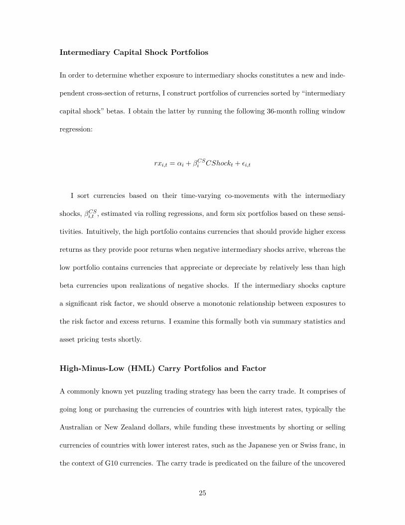
Intermediary Capital Shock Portfolios

In order to determine whether exposure to intermediary shocks constitutes a new and inde-

pendent cross-section of returns, I construct portfolios of currencies sorted by “intermediary

capital shock” betas. I obtain the latter by running the following 36-month rolling window

regression:

rxi,t = αi + βCSi CShockt + ϵi,t

I sort currencies based on their time-varying co-movements with the intermediary

shocks, βCSi,t , estimated via rolling regressions, and form six portfolios based on these sensi-

tivities. Intuitively, the high portfolio contains currencies that should provide higher excess

returns as they provide poor returns when negative intermediary shocks arrive, whereas the

low portfolio contains currencies that appreciate or depreciate by relatively less than high

beta currencies upon realizations of negative shocks. If the intermediary shocks capture

a significant risk factor, we should observe a monotonic relationship between exposures to

the risk factor and excess returns. I examine this formally both via summary statistics and

asset pricing tests shortly.

High-Minus-Low (HML) Carry Portfolios and Factor

A commonly known yet puzzling trading strategy has been the carry trade. It comprises of

going long or purchasing the currencies of countries with high interest rates, typically the

Australian or New Zealand dollars, while funding these investments by shorting or selling

currencies of countries with lower interest rates, such as the Japanese yen or Swiss franc, in

the context of G10 currencies. The carry trade is predicated on the failure of the uncovered

25

interest parity as theory suggests that higher interest rate countries’ currencies should

depreciate sufficiently to offset interest rate differentials and equate expected returns across

currencies, a prediction inconsistent with the data as the strategy yields sizeable returns.

This anomaly gives rise to the forward premium puzzle.

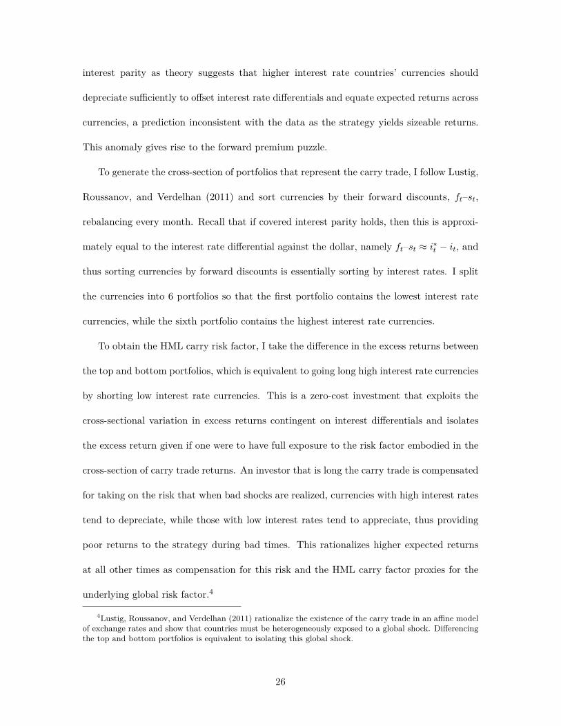
To generate the cross-section of portfolios that represent the carry trade, I follow Lustig,

Roussanov, and Verdelhan (2011) and sort currencies by their forward discounts, ft–st,

rebalancing every month. Recall that if covered interest parity holds, then this is approxi-

mately equal to the interest rate differential against the dollar, namely ft–st ≈ i∗t − it, and

thus sorting currencies by forward discounts is essentially sorting by interest rates. I split

the currencies into 6 portfolios so that the first portfolio contains the lowest interest rate

currencies, while the sixth portfolio contains the highest interest rate currencies.

To obtain the HML carry risk factor, I take the difference in the excess returns between

the top and bottom portfolios, which is equivalent to going long high interest rate currencies

by shorting low interest rate currencies. This is a zero-cost investment that exploits the

cross-sectional variation in excess returns contingent on interest differentials and isolates

the excess return given if one were to have full exposure to the risk factor embodied in the

cross-section of carry trade returns. An investor that is long the carry trade is compensated

for taking on the risk that when bad shocks are realized, currencies with high interest rates

tend to depreciate, while those with low interest rates tend to appreciate, thus providing

poor returns to the strategy during bad times. This rationalizes higher expected returns

at all other times as compensation for this risk and the HML carry factor proxies for the

underlying global risk factor.4

4Lustig, Roussanov, and Verdelhan (2011) rationalize the existence of the carry trade in an affine modelof exchange rates and show that countries must be heterogeneously exposed to a global shock. Differencingthe top and bottom portfolios is equivalent to isolating this global shock.

26

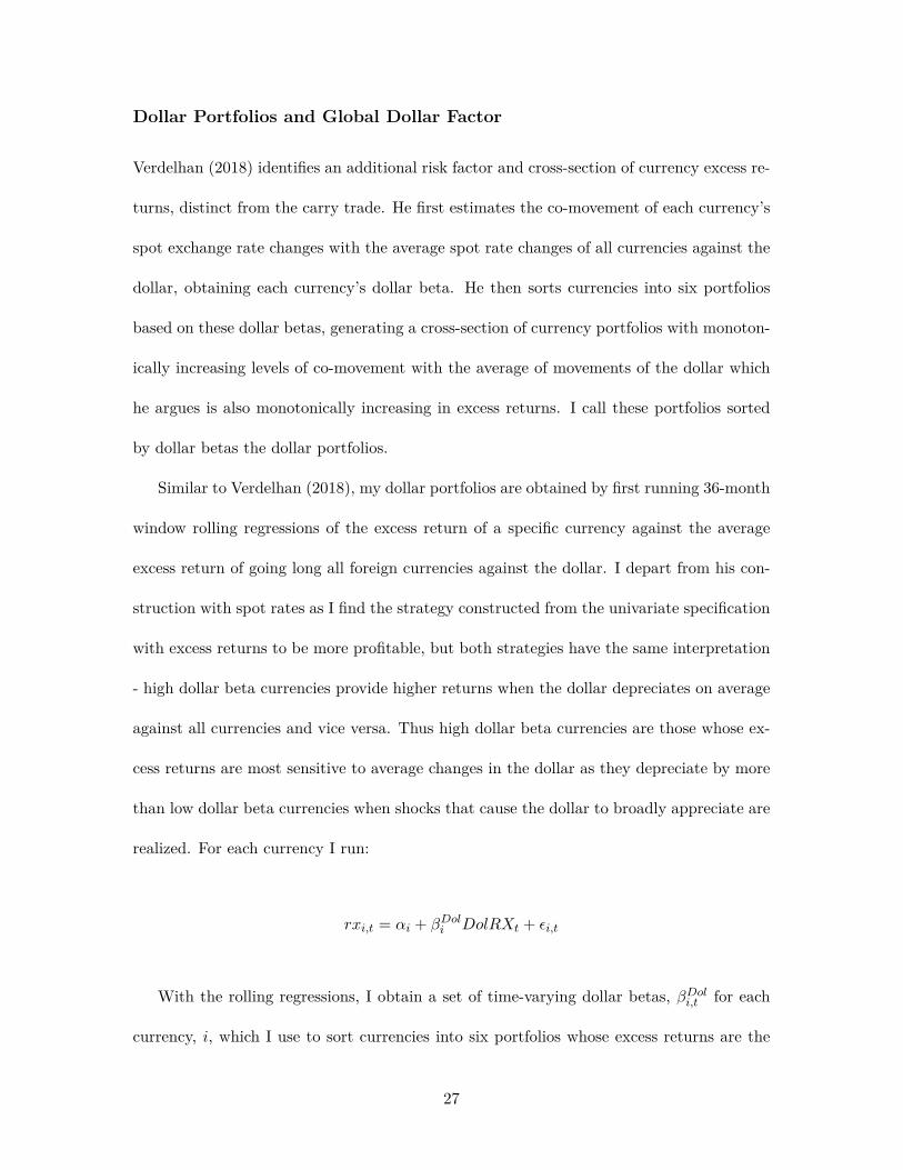
Dollar Portfolios and Global Dollar Factor

Verdelhan (2018) identifies an additional risk factor and cross-section of currency excess re-

turns, distinct from the carry trade. He first estimates the co-movement of each currency’s

spot exchange rate changes with the average spot rate changes of all currencies against the

dollar, obtaining each currency’s dollar beta. He then sorts currencies into six portfolios

based on these dollar betas, generating a cross-section of currency portfolios with monoton-

ically increasing levels of co-movement with the average of movements of the dollar which

he argues is also monotonically increasing in excess returns. I call these portfolios sorted

by dollar betas the dollar portfolios.

Similar to Verdelhan (2018), my dollar portfolios are obtained by first running 36-month

window rolling regressions of the excess return of a specific currency against the average

excess return of going long all foreign currencies against the dollar. I depart from his con-

struction with spot rates as I find the strategy constructed from the univariate specification

with excess returns to be more profitable, but both strategies have the same interpretation

- high dollar beta currencies provide higher returns when the dollar depreciates on average

against all currencies and vice versa. Thus high dollar beta currencies are those whose ex-

cess returns are most sensitive to average changes in the dollar as they depreciate by more

than low dollar beta currencies when shocks that cause the dollar to broadly appreciate are

realized. For each currency I run:

rxi,t = αi + βDoli DolRXt + ϵi,t

With the rolling regressions, I obtain a set of time-varying dollar betas, βDoli,t for each

currency, i, which I use to sort currencies into six portfolios whose excess returns are the

27

average of the excess returns of the currencies contained in each. Furthermore, following

Verdelhan (2018), I condition these portfolios by shorting portfolios if the average forward

discount of advanced economies is negative as forward discounts may contain information

about future returns.

To obtain the global dollar factor, I take the difference between the high and low dollar

beta portfolios to obtain a zero-cost investment that goes long high dollar beta currencies

and short dollar beta currencies. Differencing the two dollar portfolios purges the US-

specific information component of the dollar factor if we assume that all portfolios equally

load onto US-specific risk, and isolates the global risk factor that each currency or portfolio

is differentially exposed to in the cross-section.5 Note that in contrast to the dollar strategy

itself, I do not take into account going long or short depending on the average level of

forward discounts in order to omit information contained in the average forward discounts

and isolate the shocks that solely affect average excess returns against the dollar. Although

slightly more nuanced, the risk embodied in these portfolios is that when shocks occur that

cause the dollar to appreciate, high dollar beta currencies tend to depreciate more than low

dollar beta currencies, and thus going long the former and short the latter as a zero-cost

strategy bears the risk of poor returns in times of dollar appreciation and justifies higher

expected returns at all other times.

Momentum Portfolios

In addition to the intermediary capital, carry, and dollar portfolios, I construct a set of

momentum portfolios, following Menkhoff et al. (2012a). Currencies are ranked on their

previous month’s excess returns with the idea that winners continue their out-performance

5Verdelhan (2018) provides a full affine model that illustrates this mechanism formally.

28

while losers extend their losses. I construct six portfolios as with the other cross-sections,

with the highest portfolio containing the currencies that have the largest lagged excess

returns and vice-versa for the lowest portfolio. A momentum factor can also be extracted as

in the previous cases by taking the difference between the high and low portfolios, forming

a zero-cost strategy that goes long previously well-performing currencies and short poor

performers.

Volatility Portfolios

Menkhoff et al. (2012b) examine the carry trade from the perspective of foreign exchange

volatility, positing that carry trade returns are rationalized because the strategy performs

poorly during bouts of high volatility. I construct a measure of monthly foreign exchange

volatility as in their paper:

σFXt =

1

Tt

∑τ∈Tt

[ ∑i∈Nτ

( |∆sτ,i|Nτ

)]

where |∆τ,i| is the absolute log change in the spot rate of currency i on day τ . Tt

and Nτ signify the number of trading days in a given month and currencies on a given

day, respectively. Monthly foreign exchange volatility is equal to the monthly average of

the daily averages of absolute daily log spot changes. Volatility-sorted portfolios are then

constructed by regressing each currency’s excess returns on the residuals of an AR(1) model

of the σFXt series and sorting currencies by their past βvol

t in a series of rolling regressions,

i.e.

rxi,t = αi + βV oli V olt + ϵi,t

29

where V olt is the residual from the first order autoregression of the volatility series.6

Currencies with the largest covariances with volatility innovations should yield low ex-

cess returns as they perform similar to hedges against volatility, yielding high returns in

bouts of elevated volatility. On the other hand, currencies with little or no covariance with

volatility should yield higher excess returns as they may depreciate and pay off poorly when

volatility is elevated. Note that the pattern of excess returns and high-minus-low are con-

structed opposite all of the other portfolios as the “high” portfolio here contains currencies

with the lowest exposures and volatility betas.

Value Portfolios

Finally, I construct currency value portfolios as in Asness, Moskowitz, and Pedersen (2013).

Currencies are sorted by their value, computed as the 5-year change in purchasing power

parity (PPP) or real exchange rate (RER) given by the negative ratio of the log average

spot rate from 4.5 to 5.5 years ago and the log spot rate today less the difference in inflation

between the foreign country and the US, as measured by changes in the CPI.

V aluei,t = log

(RERi,t

RERi,t−60

)= −log(

s̄t−55,t−65

st)−

[log

(P ft

P̄t−55,t−65

)− log

(Pt

P̄t−55,t−65

)]

The intuition is that currencies with large increases in their PPP have become more un-

dervalued because higher PPP’s, equivalent to real exchange rates, imply that the domestic

currency is too weak given the relative price levels. The domestic currency eventually needs

to appreciate against the dollar in order to push the real exchange rate back to unity and

equate purchasing power across currencies, hence investing in the currency now provides

6I also construct the portfolios with the difference in the volatility series as the factor and find qualita-tively similar results.

30

good value as it will eventually appreciate and yield higher excess returns down the line.

Note that the construction of these portfolios differs from Asness, Moskowitz, and Ped-

ersen (2013) as I do not focus only on G10 currencies and generate a larger number of

portfolios, namely six versus their three.

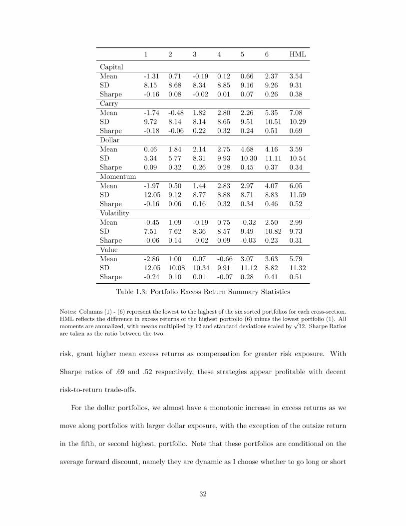
Portfolio Summary Statistics

Table 1.3 displays summary statistics for each of the portfolios described in the previous

sections. Moments are annualized and in percentage terms, namely means are multiplied

by 12, whereas standard deviations are multiplied by√12. I display each portfolio’s mean

excess return, standard deviation, and Sharpe ratio to elucidate which strategies appear to

be the most profitable before conducting the formal asset pricing tests.

The intermediary capital shock portfolios do not display monotonically increasing mean

excess returns but suggest profitability. The top portfolio indeed yields the highest mean

return of 2.4%, whereas the bottom portfolio yields a negative return of -1.3%. Combined,

a high-minus-low portfolio of going long the top and short the bottom portfolio appears

mildly profitable with a mean excess return of 3.5% per annum and a Sharpe ratio of .38.

However given the lack of a discernible pattern in mean excess returns across portfolios, it

is unlikely that intermediary capital shocks constitute their own cross-section.

The carry and momentum portfolios are almost and definitively monotonically increasing

in returns across portfolios with the high-minus-low, or zero-cost-investment, strategies

yielding mean excess returns of 7.1% and 6.1% per annum respectively. The pattern of

increasing mean excess returns supports the existence of a risk-based explanation of foreign

exchange returns as it shows that currencies with higher forward discounts or larger previous

momentum, both of which implicitly proxy for larger exposures to some source of global

31

1 2 3 4 5 6 HMLCapitalMean -1.31 0.71 -0.19 0.12 0.66 2.37 3.54SD 8.15 8.68 8.34 8.85 9.16 9.26 9.31Sharpe -0.16 0.08 -0.02 0.01 0.07 0.26 0.38CarryMean -1.74 -0.48 1.82 2.80 2.26 5.35 7.08SD 9.72 8.14 8.14 8.65 9.51 10.51 10.29Sharpe -0.18 -0.06 0.22 0.32 0.24 0.51 0.69DollarMean 0.46 1.84 2.14 2.75 4.68 4.16 3.59SD 5.34 5.77 8.31 9.93 10.30 11.11 10.54Sharpe 0.09 0.32 0.26 0.28 0.45 0.37 0.34MomentumMean -1.97 0.50 1.44 2.83 2.97 4.07 6.05SD 12.05 9.12 8.77 8.88 8.71 8.83 11.59Sharpe -0.16 0.06 0.16 0.32 0.34 0.46 0.52VolatilityMean -0.45 1.09 -0.19 0.75 -0.32 2.50 2.99SD 7.51 7.62 8.36 8.57 9.49 10.82 9.73Sharpe -0.06 0.14 -0.02 0.09 -0.03 0.23 0.31ValueMean -2.86 1.00 0.07 -0.66 3.07 3.63 5.79SD 12.05 10.08 10.34 9.91 11.12 8.82 11.32Sharpe -0.24 0.10 0.01 -0.07 0.28 0.41 0.51

Table 1.3: Portfolio Excess Return Summary Statistics

Notes: Columns (1) - (6) represent the lowest to the highest of the six sorted portfolios for each cross-section.HML reflects the difference in excess returns of the highest portfolio (6) minus the lowest portfolio (1). Allmoments are annualized, with means multiplied by 12 and standard deviations scaled by

√12. Sharpe Ratios

are taken as the ratio between the two.

risk, grant higher mean excess returns as compensation for greater risk exposure. With

Sharpe ratios of .69 and .52 respectively, these strategies appear profitable with decent

risk-to-return trade-offs.

For the dollar portfolios, we almost have a monotonic increase in excess returns as we

move along portfolios with larger dollar exposure, with the exception of the outsize return

in the fifth, or second highest, portfolio. Note that these portfolios are conditional on the

average forward discount, namely they are dynamic as I choose whether to go long or short

32

the currencies against the dollar depending on if the average forward discount is positive

or negative, respectively. The top portfolio has a mean excess return of 4.2%, while the

high-minus-low yields 3.6% per annum with a Sharpe ratio of .34. In contrast to the carry

and momentum portfolios, the high-minus-low does worse than simply going long the top

portfolio as shorting the bottom portfolio does not yield additional returns.

The top volatility portfolio contains currencies that are the least exposed to foreign

exchange volatility and exhibits the highest returns compared to those that are relatively

more exposed.7 This is in line with intuition as the currencies in the bottom portfolio,

which have the higher volatility betas, tend to provide higher returns when volatility is

high, and thus serve as insurance or a hedge that should yield lower excess returns at all

other times. The high-minus-low yields a mean excess return of 3% with a Sharpe ratio of

.31, improving upon the return of only the top portfolio due to the shorting of the bottom

portfolio.

Finally for the value portfolios, while we do not obtain a strict monotonic pattern in

excess returns, we observe a significant spread between the high and low portfolios. The

best value portfolio yields a mean excess return of 3.6% per annum, while the worst value

portfolio performs poorly with a mean loss of 2.9% per annum. The high-minus-low thus

provides significant mean excess returns at 5.8% and a Sharpe ratio of .51, comparable to

the momentum cross-section.

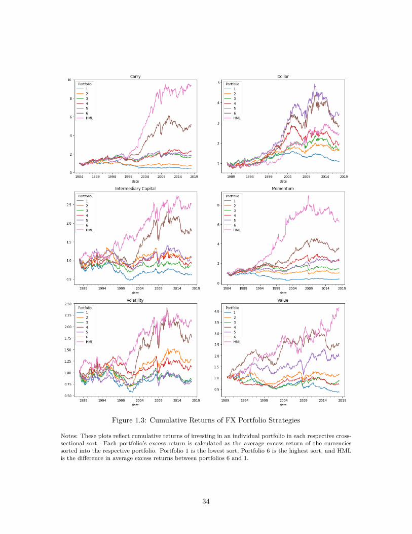
Figure 1.3 displays the cumulative returns from investing $1 in each portfolio. As was

suggested by the summary statistics, an investor would have increased their initial in-

vestments to under $10 and a little over $6 if following the carry trade and momentum

7Recall that the top volatility portfolio, namely portfolio 6, contains currencies with the lowest volatilitybetas, whereas the bottom portfolio contains those with the highest volatility betas. I use this conventionto remain consistent with the other portfolios in which the top portfolio contains risky currencies, while thebottom has the least risky.

33

Figure 1.3: Cumulative Returns of FX Portfolio Strategies

Notes: These plots reflect cumulative returns of investing in an individual portfolio in each respective cross-sectional sort. Each portfolio’s excess return is calculated as the average excess return of the currenciessorted into the respective portfolio. Portfolio 1 is the lowest sort, Portfolio 6 is the highest sort, and HMLis the difference in average excess returns between portfolios 6 and 1.

34

high-minus-low strategies, respectively. Furthermore for the cross-section of carry and mo-

mentum portfolios, the cumulative returns appear to almost be monotonically increasing

across portfolios, in line with the summary statistics. This builds support for the existence

of a risk-based explanation for the cross-section of returns as it appears that increased load-

ings or exposure to potential risk factors and shocks are associated with consistently higher

returns.

Cumulative returns to the dollar strategy are less impressive, as the initial outlay in-

creases to a little less than three-fold by 2014 before declining persistently since then. An

investor would have been better off only going long the top portfolios as indicated by the

larger cumulative and excess returns without shorting the bottom portfolio, which recall

has positive mean excess returns and erodes profitability. All portfolios however decline

from 2015 onwards, presumably due to dollar appreciation.

The intermediary capital portfolios do not display monotonicity in terms of cumulative

returns, but the high-minus-low portfolio does steadily increase the initial outlay 2.5 times

over the sample period. The cumulative return peaks in 2015 before sharply dropping and

stagnating since then. The volatility portfolios display mild capital gains up until 2009 in

which we observe a sharp drop for all portfolios. There is a recovery following this sharp

drop, but returns essentially stagnate from then on.

Cumulative returns from the value strategy appear consistently profitable, although not

to the magnitude of the carry and momentum strategies. An initial investment increases

four fold by the end of the sample, but note the periods of persistent declines, most notably

from 2004 to 2007, 2010 to 2012, and 2014 to 2015. In contrast to all other strategies, the

value strategy is unique in consistently being profitable over the past 3 years.8

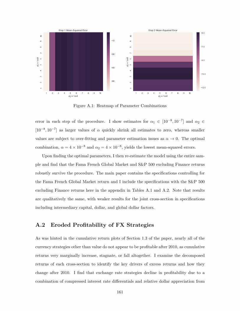
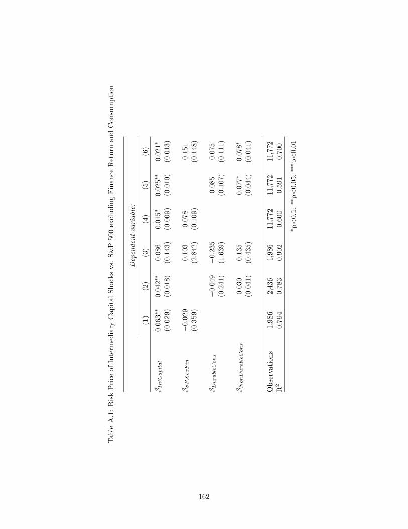
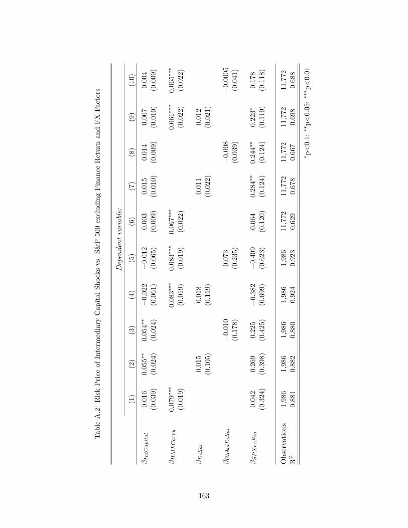
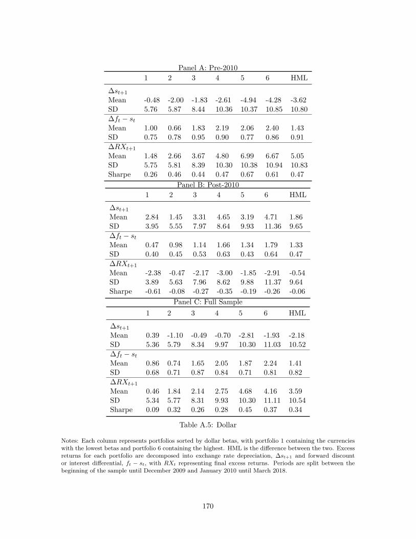
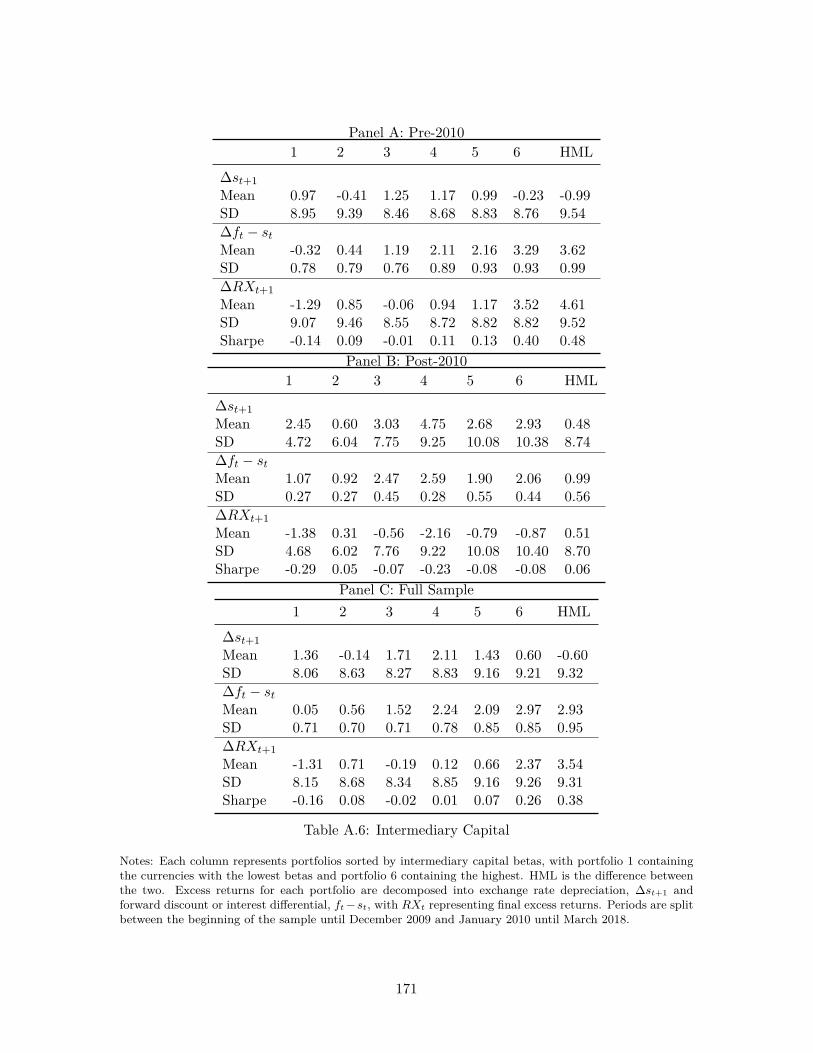
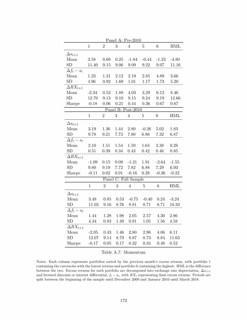
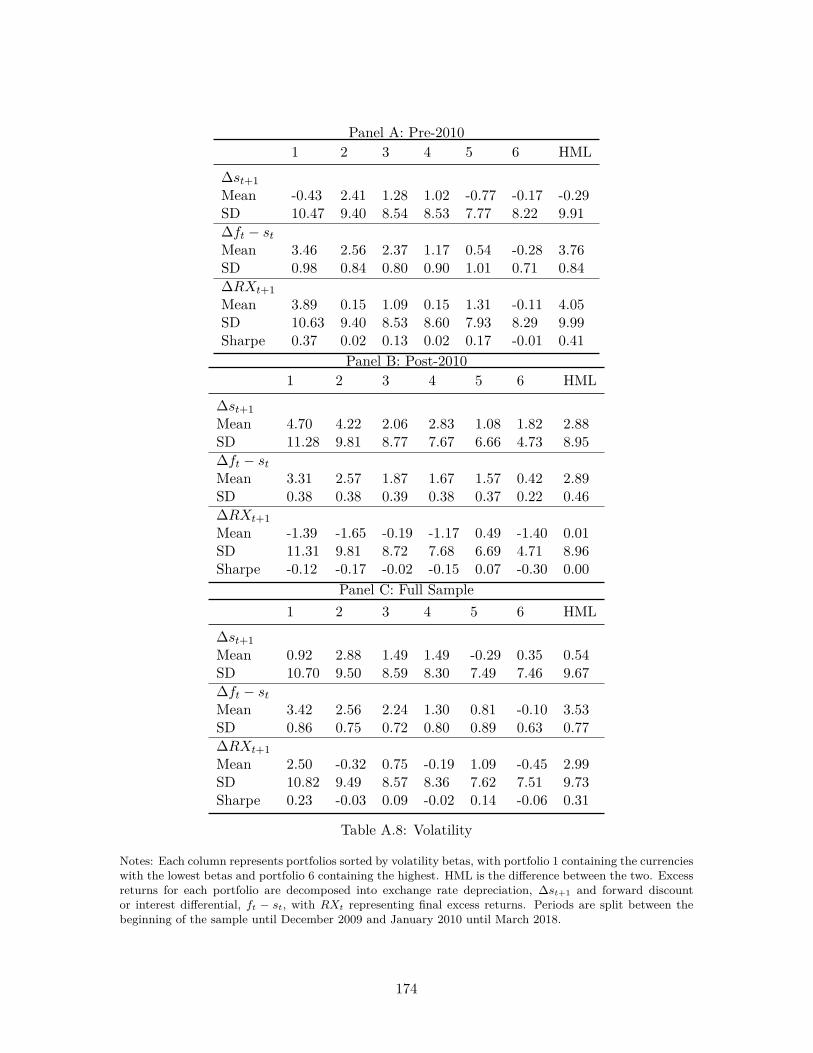
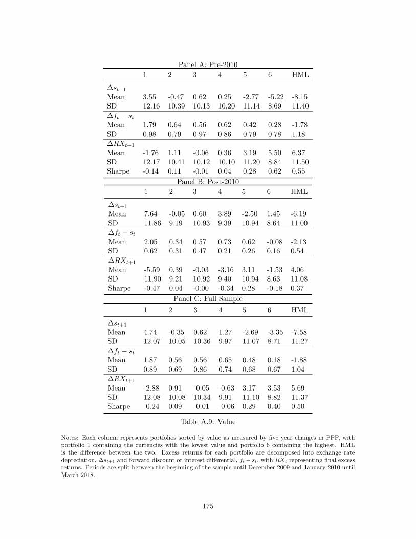
8Note that nearly all of the strategies except value appear to reach peaks in 2010 and have not beennearly as profitable since then. I examine this further in the Appendix A.2 by deconstructing portfolio

35

1.4 Empirical Results

I shift now to a formal empirical analysis of the relationship between intermediary capital

and exchange rate movements. I begin with a brief analysis of exchange rate movements

with the intermediary capital shocks and the HML carry and dollar factors to assess whether

currencies exhibit the predicted patterns, namely whether risky currencies depreciate and

safe haven currencies appreciate when negative capital shocks are realized. I then proceed

to conduct asset pricing tests to evaluate the relevance of intermediary capital compared to

the market return and consumption growth. My findings align with the theoretical predic-

tions outlined in the introduction and literature review in Sections 1.1 and 1.2, supporting

the central role of financial intermediaries in exchange rate determination and providing

evidence in favor of open economy, intermediary-based asset pricing models.

The latter part of this section examines the interplay of intermediary capital with the

HML carry, dollar, and global dollar factors. My asset pricing tests display the dominance

of the HML carry factor as a significant source of risk for exchange rates and the sub-

sumption of intermediary capital risk upon inclusion of the HML carry factor suggests that

intermediary capital risk is one of the many sources of risk embedded within the HML carry

factor. My results with the dollar and global dollar factor maintain the relevance of finan-

cial intermediaries, and show that the global component of dollar risk, as isolated by the

global dollar factor, significantly prices the joint cross-section of exchange rate portfolios.

returns into interest rate and exchange rate depreciation components for the pre- and post-2010 periodsfor each cross-section and find that a combination of compressed interest rate differentials and unfavorabledollar appreciation lead to declines in currency strategy returns.

36

Spot Changes and Intermediary Shocks

I first examine whether intermediary capital shocks contain any information content beyond

that held in the spot changes of the HML carry and dollar factors. The former takes the

difference between exchange rate changes of the currencies with the largest and smallest

forward discounts, which proxy for interest rate differentials, while the latter reflects the

average of all exchange rate changes against the dollar. I estimate the following for each

currency:

∆si,t = αi + βHMLi HML−i,t + βDol

i Dol−i,t + βCSi CShockt + ϵi,t (1.3)

Note that HML−i,t and Dol−i,t exclude the currency on the left-hand-side to avoid

regressing on the same variable. This regression estimates the size and direction of exchange

rate movements with respect to systematic variation. For example, if the dollar on average

appreciates by one percent, βDoli yields the amount country i’s currency depreciates in

percentage terms.

The results for the G11 currencies are displayed in Table 1.4. Column (1) displays

the sensitivities of exchange rate movements to the risks contained within carry trade as

measured by spot rate movements. We observe a positive co-movement of traditionally risky

currencies, such as the Australian and New Zealand dollars, with that of the carry trade,

namely when the carry trade appreciates, these currencies do as well, in line with intuition.

Similarly for traditional safe haven, low interest rate currencies such as the Japanese yen

and Swiss franc, we observe negative coefficients, suggesting that these currencies appreciate

when the carry trade is depreciating.

Column (2) displays the systematic co-movements of currencies with the average changes

37

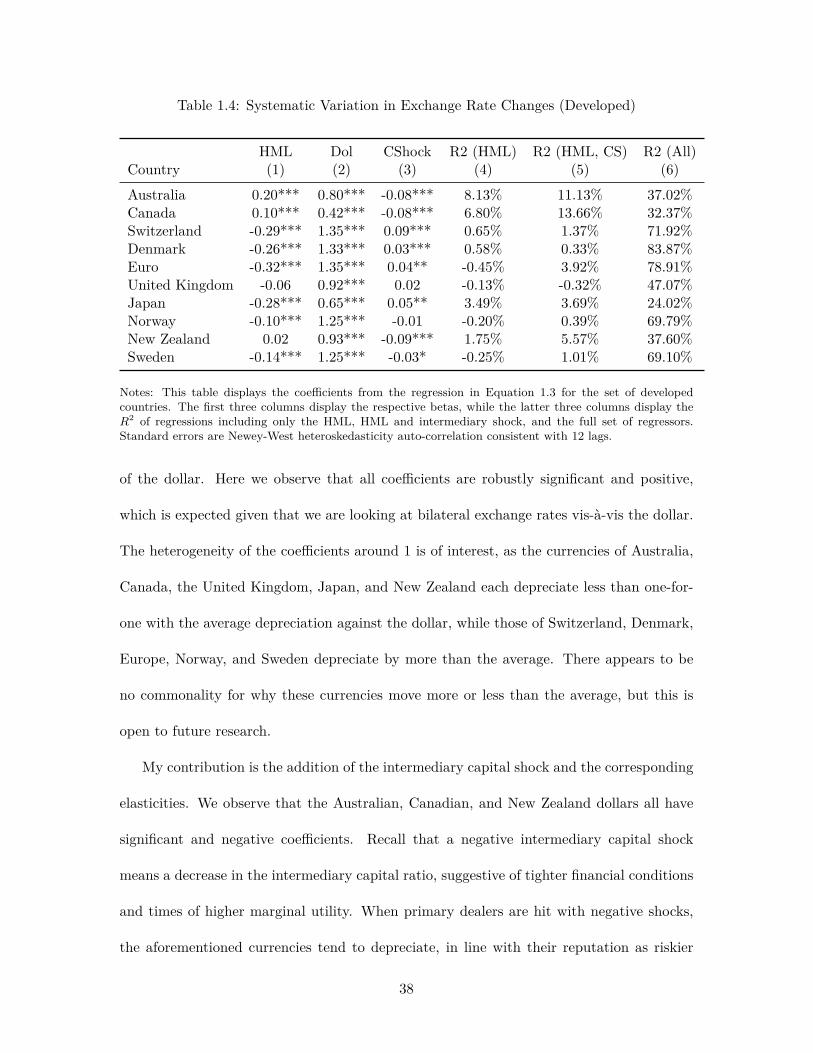
Table 1.4: Systematic Variation in Exchange Rate Changes (Developed)

HML Dol CShock R2 (HML) R2 (HML, CS) R2 (All)Country (1) (2) (3) (4) (5) (6)Australia 0.20*** 0.80*** -0.08*** 8.13% 11.13% 37.02%Canada 0.10*** 0.42*** -0.08*** 6.80% 13.66% 32.37%Switzerland -0.29*** 1.35*** 0.09*** 0.65% 1.37% 71.92%Denmark -0.26*** 1.33*** 0.03*** 0.58% 0.33% 83.87%Euro -0.32*** 1.35*** 0.04** -0.45% 3.92% 78.91%United Kingdom -0.06 0.92*** 0.02 -0.13% -0.32% 47.07%Japan -0.28*** 0.65*** 0.05** 3.49% 3.69% 24.02%Norway -0.10*** 1.25*** -0.01 -0.20% 0.39% 69.79%New Zealand 0.02 0.93*** -0.09*** 1.75% 5.57% 37.60%Sweden -0.14*** 1.25*** -0.03* -0.25% 1.01% 69.10%

Notes: This table displays the coefficients from the regression in Equation 1.3 for the set of developedcountries. The first three columns display the respective betas, while the latter three columns display theR2 of regressions including only the HML, HML and intermediary shock, and the full set of regressors.Standard errors are Newey-West heteroskedasticity auto-correlation consistent with 12 lags.

of the dollar. Here we observe that all coefficients are robustly significant and positive,

which is expected given that we are looking at bilateral exchange rates vis-à-vis the dollar.

The heterogeneity of the coefficients around 1 is of interest, as the currencies of Australia,

Canada, the United Kingdom, Japan, and New Zealand each depreciate less than one-for-

one with the average depreciation against the dollar, while those of Switzerland, Denmark,

Europe, Norway, and Sweden depreciate by more than the average. There appears to be

no commonality for why these currencies move more or less than the average, but this is

open to future research.

My contribution is the addition of the intermediary capital shock and the corresponding

elasticities. We observe that the Australian, Canadian, and New Zealand dollars all have

significant and negative coefficients. Recall that a negative intermediary capital shock

means a decrease in the intermediary capital ratio, suggestive of tighter financial conditions

and times of higher marginal utility. When primary dealers are hit with negative shocks,

the aforementioned currencies tend to depreciate, in line with their reputation as riskier

38

currencies as they yield poor returns when intermediaries need them most. In terms of

economic magnitude, a one standard deviation intermediary capital shock is associated with

approximately a half of a percent in depreciation. In contrast, if we instead look at the haven

currencies, namely the Japanese yen and Swiss franc, we observe positive coefficients, with

economic magnitudes of a quarter and a half percent appreciation respectively. Consistent

with intuition, safe haven currencies tend to appreciate when negative intermediary capital

shocks hit.

Columns (4)–(6) display the R2’s of the regressions with only the HML, HML and

intermediary capital shock, and the full specification, respectively. We can see that the

intermediary capital shock adds some explained variation, suggesting that intermediary

capital shocks provide some additional information content above and beyond that of the

carry trade itself. The full specification has quite high R2’s of up to 83% for the Danish

krone and 78% for the euro, showing that average changes in the dollar account for an

outsize portion of exchange rate movements, as found by Verdelhan (2018). In other words,

currencies appear to share a large amount of systematic variation as a lot of their movements

are linked to broad movements of the dollar against all currencies.

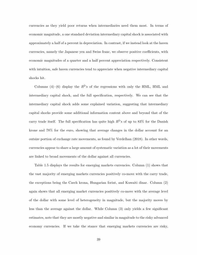
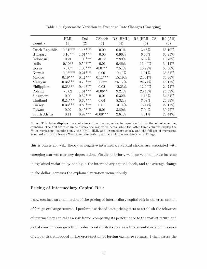
Table 1.5 displays the results for emerging markets currencies. Column (1) shows that

the vast majority of emerging markets currencies positively co-move with the carry trade,

the exceptions being the Czech krona, Hungarian forint, and Kuwaiti dinar. Column (2)

again shows that all emerging market currencies positively co-move with the average level

of the dollar with some level of heterogeneity in magnitude, but the majority moves by

less than the average against the dollar. While Column (3) only yields a few significant

estimates, note that they are mostly negative and similar in magnitude to the risky advanced

economy currencies. If we take the stance that emerging markets currencies are risky,

39

Table 1.5: Systematic Variation in Exchange Rate Changes (Emerging)

HML Dol CShock R2 (HML) R2 (HML, CS) R2 (All)Country (1) (2) (3) (4) (5) (6)Czech Republic -0.31*** 1.48*** -0.00 0.01% 3.48% 65.10%Hungary -0.16*** 1.61*** -0.00 0.96% 6.60% 66.25%Indonesia 0.21 1.00*** -0.12 2.89% 5.32% 10.76%India 0.10** 0.50*** -0.01 9.46% 11.46% 34.14%Korea -0.07 1.06*** -0.07** 7.51% 16.29% 53.56%Kuwait -0.05*** 0.21*** 0.00 -0.40% 1.01% 36.51%Mexico 0.19*** 0.47*** -0.11*** 15.19% 24.91% 34.36%Malaysia 0.36*** 0.70*** 0.05** 25.17% 24.74% 48.17%Philippines 0.23*** 0.44*** 0.02 12.23% 12.06% 24.74%Poland -0.02 1.61*** -0.06** 9.21% 20.46% 74.59%Singapore 0.00 0.52*** -0.01 0.32% 1.15% 54.34%Thailand 0.24*** 0.66*** 0.04 8.32% 7.98% 24.39%Turkey 0.33*** 0.83*** 0.01 13.14% 13.44% 29.17%Taiwan 0.02 0.45*** -0.01 3.80% 7.04% 39.25%South Africa 0.11 0.99*** -0.08*** 2.61% 4.81% 28.44%

Notes: This table displays the coefficients from the regression in Equation 1.3 for the set of emergingcountries. The first three columns display the respective betas, while the latter three columns display theR2 of regressions including only the HML, HML and intermediary shock, and the full set of regressors.Standard errors are Newey-West heteroskedasticity auto-correlation consistent with 12 lags.

this is consistent with theory as negative intermediary capital shocks are associated with

emerging markets currency depreciation. Finally as before, we observe a moderate increase

in explained variation by adding in the intermediary capital shock, and the average change

in the dollar increases the explained variation tremendously.

Pricing of Intermediary Capital Risk

I now conduct an examination of the pricing of intermediary capital risk in the cross-section

of foreign exchange returns. I perform a series of asset pricing tests to establish the relevance

of intermediary capital as a risk factor, comparing its performance to the market return and

global consumption growth in order to establish its role as a fundamental economic source

of global risk embedded in the cross-section of foreign exchange returns. I then assess the

40

significance of intermediary capital risk in combination with the HML carry, dollar, and

global dollar factors to shed light upon its relationship with these exchange rate factors.

I show the following in turn: First, intermediary capital shocks provide an economic

source of risk that underpins the carry trade, robust to the inclusion of consumption growth

which reflects the relevance of financial intermediaries’ pricing kernels over those of house-

holds. Although intermediary capital shocks do not constitute their own, independent

cross-section of returns, the results show that they do matter for the carry trade and the

joint cross-section of all currency portfolios. Second, the HML carry factor subsumes the

risk embedded in the intermediary capital shocks and prices both the carry trade and the

entire cross-section of currency portfolios, pointing towards intermediary capital risk as a

component of the broader HML carry risk. In addition, the global component of the dollar

factor as a proxy for global shocks independent of those contained within the HML carry

factor matters for the cross-section of excess returns, whereas the dollar factor, un-purged

of US-specific risk, does not.

My estimation of the prices of risk follows the standard two-stage Fama-MacBeth pro-

cedure. In the first stage, for each test portfolio I run a time series regression of its excess

returns on a constant and the candidate risk factors to obtain a set of portfolio-specific

betas. Formally:

rxi,t = αi + βi’ft + ϵi,t for i = 1, ..., N (1.4)

where ft is a vector of factors and βi is the vector of factor loadings for portfolio i, and

N is the number of test portfolios. In the second stage, I estimate the prices of risk by

running a cross-sectional regression for each time period t and take the average to obtain

the final estimates:

41

rxi,t = λtβi’+ νi,t for t = 1,…, T (1.5)

The coefficient of interest is λ̂ =∑

λ̂t/T , namely the vector of risk prices for each

factor. I estimate the first stage betas with ordinary least squares, and compute the second

stage risk prices using the pooled mean group estimator. Per Burnside’s (2011) critique of

Lustig and Verdelhan (2007), I construct GMM standard errors following Cochrane (2005)

to alleviate concerns about standard errors as our second stage regressors, namely the first

stage betas, are estimated.9

Before diving into the results, note that in contrast to previous studies that use the US

market return, I employ the Fama French global market return as my control risk factor. I

utilize the Feng et al. (2017) two-pass procedure which employs machine learning techniques

as the immense number of pre-existing factors in the empirical asset pricing literature make

the selection of baseline factors both tedious and inconsistent given the difference in esti-

mates depending on which factors are included in the asset pricing regressions. I perform

this control factor selection procedure as empirical asset pricing studies for exchange rates

have not yet carefully found the correct factors to serve as controls in baseline specifica-

tions, making studies generally incomparable. I fill this void by formally identifying the

Fama French global market return as the most relevant control factor in comparison to

other factors for exchange rates, and argue that future studies of exchange rate risk factors

9Another option is the Shanken (1992) correction. Suppose we have N test portfolios, K factors, and Tperiods. Per Cochrane (2005), the Shanken corrected variance-covariance is computed as:

V =1

T

((β′β)−1β′Σβ(β′β)−1(1 + λ′Σ−1

f λ) + Σf

)where β′ is an N × K matrix containing the estimated betas from the first stage in Equation ??, Σ =

Cov(ϵ′t,′ ϵt) is the N×N variance-covariance matrix of the residuals from Equation 1.4, λ′ is an K×1 vector

of the estimated average risk prices from Equation 1.5, and Σf = Cov(f ′t , ft) is theK×K variance-covariance

matrix of the factors.

42

should always be compared to this baseline.10 Interested readers are encouraged to refer to

Appendix A.1 where I provide a full discussion of the factor selection procedure.

Intermediary Capital as an Economic Risk Factor

Table 1.6 displays the results from the asset pricing tests of intermediary capital shocks

with the global market return and consumption growth to examine the relevance of financial

intermediary capital risk in the pricing of foreign exchange risk. I depart from the previous

literature by using the Fama French global market return given its survival in the factor

selection procedure, and also employ a wider set of exchange rate portfolios when testing

for the significance of intermediary capital risk.11

Column (1) shows the risk prices estimated on the cross-section of six currency portfolios

sorted by intermediary capital shock betas. If intermediary capital risk constitutes its own

cross-section of excess returns, I expect a significant and positive price of intermediary

capital risk as currencies that depreciate upon realizations of negative intermediary capital

shocks provide lower excess returns at bad times and are thus deemed risky, compensating

investors for the aforementioned risk by providing higher expected returns at all other times.

We do not observe a significant price of intermediary capital risk or the global market, thus

eliminating the existence of this independent cross-section of exchange rate excess returns.

However moving to Column (2), we observe a significant price of intermediary risk for

the cross-section of carry trade portfolios sorted by forward discounts. Intermediary capital

10My selection procedure also highlights the S&P 500 excluding financials as a factor, but for parsimony Ionly include the results with the global market return given the limited number of test portfolios, especiallyfor the carry trade. The results with this other control factor in lieu of the global market are included inthe Appendix A.1 and results are similar.

11He, Kelly, and Manela (2017) test their factor against the carry trade and momentum portfolios fromLettau, Maggiori, and Weber (2014) and Menkhoff et al. (2012), finding significant and positive prices ofrisk. I augment their results by extending the sample period up to the end of 2017 and testing on a widerset of currency portfolios to capture additional cross-sections of exchange rates from the literature.

43

Table1.6:

Risk

Priceof

Interm

ediary

Cap

italS

hocksvs.Globa

lMarketReturnan

dCon

sumption

Interm

ediary

Cap

ital

Carry

Trad

eAllCross-Sectio

ns(1)

(2)

(3)

(4)

(5)

(6)

(7)

βIntC

apital

0.01

10.05

9∗∗∗

0.04

2∗∗

0.07

90.02

6∗∗

0.02

5∗∗

0.02

3∗(0.012

)(0.022

)(0.018

)(0.079

)(0.011

)(0.010

)(0.014

)

βFFGloba

lMkt

0.06

60.20

20.32

60.10

7∗0.15

4∗∗

(0.080

)(0.136

)(0.637

)(0.057

)(0.069

)

βDurableC

ons

−0.04

9−0.23

70.08

50.08

4(0.241

)(0.942

)(0.107

)(0.093

)

βNonDurableC

ons

0.03

00.11

80.07

7∗0.07

9∗∗

(0.041

)(0.309

)(0.044

)(0.033

)

Observatio

ns1,96

81,96

82,43

61,96

811

,772

11,772

11,772

R2

0.84

00.80

80.78

30.90

40.62

50.59

10.71

2

Not

e:∗ p<0.1;

∗∗p<

0.05

;∗∗∗p<

0.01

Notes:Thistabledisplays

estim

ates

oftheris

kprices

from

thesecond

stag

eof

theFa

maMacBethregressio

n.Colum

n(1)displays

results

forthecross-sectionof

interm

ediary

capitals

hock

beta

sorted

portfolio

s,Colum

ns(2)-(4)exam

inethecarrytrad

e,an

dColum

ns(5)-(7)show

estim

ates

ontheentir

ejointcross-section

ofcu

rren

cystrategy

portfolio

s.The

first

stag

etim

eserie

sregressio

nis

estim

ated

foreach

portfolio

byordina

ryleastsqua

res,

while

thesecond

stag

einvolves

across-sectiona

lregressionforeach

time,

tof

excess

returnson

estim

ated

betasacross

allt

estassets/p

ortfolios.

Iem

ploy

thesecond

stag

eusingthepo

oled

mean

grou

psestim

ator.Stan

dard

errors

areconstruc

tedfollo

wingtheGMM

metho

dology

asin

Cochran

e(200

5).

44

risk is priced into the carry trade at 5.9% per annum, implying that high interest rate

currency portfolios have high intermediary capital betas as their returns more positively

co-move with the intermediary capital shocks, and are thus compensated for the risk of low

returns when intermediary capital erodes. This provides support for intermediary capital

as a fundamental economic source of risk embedded in exchange rates and provides an

explanation for the forward premium puzzle as investors appear to be rewarded for holding

high interest rate currencies that run the risk of depreciation when intermediary capital

declines. Notice that intermediary capital risk is priced despite the presence of the global

market return showing that it contains more information than equity prices - I interpret this

as reflecting the outsize importance of intermediary capital as proxying for the risk-bearing

capacity of relevant financial intermediaries that theory suggests.

This result is not limited to the cross-section of the carry trade - it also holds for the

joint cross-section of all currency portfolios. Column (5) displays the risk price estimates

from the sample that simultaneously employs all of the constructed portfolios, namely

intermediary capital, carry, dollar, momentum, volatility, and value as described in Section

1.3, each of which presumably captures different sources of risk premia and anomalies in

exchange rates. I find a significant price of intermediary capital risk at 2.6% per annum.

While smaller in magnitude than the estimate from the carry trade portfolios alone, this

finding supports the importance of intermediary capital in the pricing of exchange rates as

using the broader set of portfolios identifies one systematic economic source of global risk

that is embedded within a wide range of exchange rate risk premia, invariant to the type

of sorting and portfolio construction. Furthermore given the low excess returns of all other

cross-sections of exchange rates, it is not surprising that I obtain a smaller estimate.12

12I also test each cross-section independently in the online appendix. None of the other cross-sectionsof foreign exchange returns exhibit significant intermediary capital risk prices when estimated individually,

45

An additional finding is the significance of the global market return for the entire cross-

section of foreign exchange returns at 10.7% per annum. Previous studies have had difficul-

ties explaining exchange rate excess returns with the market return (Daniel, Hodrick, and

Lu 2017), but I find that it is global market risk that may be the relevant factor, at least for

the wider cross-section of exchange rate excess returns. The significance of this estimate

is in line with its relevance as a baseline control factor and supports the two-stage factor

selection procedure.

The significance of the intermediary capital shock for the risk pricing of the carry trade

and the wider cross-section of foreign exchange excess returns leads one to question whether

it is a distinct economic source of risk independent of the consumption growth risk found

by Lustig and Verdelhan (2007). One could argue that intermediaries are just a veil for

households and that intermediary capital risk may just proxy for household consumption

growth risk. If this is true, models with financial intermediaries may then be adding an

additional layer of complexity that is not necessarily warranted. I examine this notion by

performing my asset pricing tests with US durable and non-durable consumption growth

as additional risk factors to determine whether it is consumption growth, intermediary

shocks, or a combination of the two that account for excess returns in exchange rates. This

exercise clarifies the relevance of financial intermediaries versus households in the pricing

of exchange rates.

Column (3) of Table 1.6 displays the results from the Fama MacBeth regressions with

intermediary capital shocks and durable and non-durable US consumption growth as risk

factors for the carry trade. I find that intermediary risk is still significant and positively

priced at 4.2% per annum, while the consumption growth factors are not priced. My

but this could be due to the depressed returns in the past decade.

46

results show that intermediary capital risk is more important than household consumption

risk in explaining the carry trade as investors appear to be compensated for co-movement of

exchange rate returns with fluctuations in the financial intermediaries’ pricing kernel rather

than that of households. My findings validate the notion that open economy models require

constrained intermediaries at the center of asset markets in order to account for the failure

of the UIP and existence of the forward premium puzzle as the prediction and pattern of

high interest rate currencies more positively co-varying with intermediary capital and thus

subject to larger relative depreciations upon the realization of negative intermediary capital

shocks is borne out in the data.

This finding is again extended to the entire cross-section of foreign exchange portfolios as

indicated in Column (6). As before, we find a smaller, but significant price of intermediary

risk at 2.5% per annum, verifying the robust importance of intermediary capital risk for

the joint cross-section of exchange rate returns. In contrast to estimates with the carry

trade alone, I also obtain a positive and significant price of non-durable consumption risk,

providing support for Lustig and Verdelhan’s (2007) original finding. However given the

significance of intermediary risk for both carry and entire cross-sections, I interpret this as

highlighting the larger importance of the financial intermediary’s pricing kernel over that

of the households. It is important to keep in mind that I am not claiming that households

are completely irrelevant to pricing exchange rates or asset pricing in general, merely that

financial intermediaries may the be more relevant marginal investor given the recent success

of the theory and my more robust findings in support of intermediary capital risk. My

results provide support for the importance of including constrained financial intermediaries

in open economy macro-economic models in order to reconcile some of the inconsistencies

between the theory and data.

47

Columns (4) and (7) serve as robustness checks by controlling for the global market

return as well. For the carry trade I find that in contrast to before, none of the factors are

now significant as displayed in Column (4). However, I rationalize this finding in two ways:

first, note that the global market return is correlated with the intermediary capital shocks

as displayed in Table 1.2 and thus its inclusion may dilute the significance of intermediary

capital risk, especially if the relevant components of consumption growth and the capital

shocks are also partially contained within the global market return. Second, given that I

only have six portfolios in the carry trade cross-section, the regression has almost as many

regressors as test portfolios - the risk prices may then be mis-estimated and the lack of

significance may be a by-product of this.13

On the other hand, the full specification in Column (7) for the joint cross-section retains

the significance of intermediary capital risk. Risk prices are presumably more precisely es-

timated in this larger sample given the increased number of portfolios and I find that

intermediary capital is again a significant and positively priced risk factor for exchange

rates at 2.3% per annum. The risk price of intermediary capital decreases in the level of

significance, which I attribute to dilution due to the inclusion of the global market return,

which is also significantly priced at 15.4% per annum. Given that non-durable consumption

growth remains significantly priced, my results thus suggest that while financial intermedi-

aries have the more robust pricing kernels, the risk embedded in consumption growth also

plays a role, consistent with Lustig and Verdelhan (2007) and intuition as one would expect

real shocks to be relevant for a wider set of exchange rate risk premia.

To visualize the effectiveness of intermediary capital in pricing the cross-sections of for-

13I have also run specifications with only one type of consumption growth risk that include the globalmarket return. I find significance for intermediary capital risk in the specification with only intermediarycapital shocks, non-durable consumption growth, and the Fama French global market return.

48

Figure 1.4: Carry Trade Mean Excess Returns and Intermediary Capital Betas

This figure displays the mean excess returns of each portfolio of the carry trade cross-section, namelycurrencies sorted on forward discounts. The x-axis contains intermediary capital betas, estimated for eachportfolio by regressing its excess returns across the whole sample on a constant and the intermediary capitalshock. The line reflects the best fit for the relationship between average portfolio returns and betas.

eign exchange, Figures 1.4 and 1.5 display scatter plots of mean portfolio returns against

intermediary capital betas. Figure 1.4 shows that the carry trade portfolios are monotoni-

cally increasing both in mean excess returns and intermediary capital betas, implying that

the carry trade and forward premium puzzle may be explained through the lens of inter-

mediary capital risk as it is apparent that higher interest rate currencies are precisely those

that are more exposed to intermediary capital shocks. These currencies enjoy higher excess

returns because their larger co-movement with intermediary capital leads to depreciations

and losses when intermediary capital erodes, coinciding with times of high intermediary

marginal utility that require increased compensation and risk premia for downside risk.

49

Figure 1.5 displays the analogous plot for the joint cross-section of all currency portfo-

lios. I obtain a similar pattern as with the carry portfolios - high portfolios enjoy higher

excess returns and coincide with larger intermediary capital betas, while lower portfolios

yield lower excess returns and have lower and even negative intermediary capital betas.

Risky currency portfolios are again those that exhibit larger mean excess returns which are

rationalized by relatively larger co-movements with intermediary capital, while the safer

currency portfolios exhibit low or even negative co-movement with intermediary capital,

in line with the intuition that currencies which appreciate upon the realization of negative

intermediary capital shocks serve as hedges and should provide lower returns. Although not

strict, I do observe a generally monotonic relationship between portfolios and intermediary

capital betas as the bottom left, middle, and top right of the plot contain the low and less

risky, intermediate, and high and most risky portfolios, respectively.

It is important to note that this pattern holds despite the different measures upon which

each cross-section is sorted and constructed. The robust pattern between intermediary

capital betas and portfolio excess returns is invariant to the sorting characteristic, lending

credence to the notion that intermediary capital risk in fact underpins a wide set of exchange

rate risk premia and thus serves a systematic source of global risk. Currency portfolios that

are deemed as risky due to their larger exposure to risk factors are also more exposed to

fluctuations in intermediary capital, implying that intermediary capital risk is embedded

and compensated for in a variety of cross-sections of exchange rates and risk premia.

In summary, I have found that intermediary capital shocks are a significantly priced risk

factor for the cross-section of carry trade returns and the wider cross-section of all currency

portfolio returns. My results point towards the central role that financial intermediaries

play in open economy models in order to give rise to deviations in the UIP and the forward

50

Figure 1.5: Mean Excess Returns and Intermediary Capital Betas

This figure displays the mean excess returns of each portfolio of the joint cross-section of exchange rates,which includes six portfolios for intermediary capital, carry, dollar, momentum, volatility, and value. Thex-axis contains intermediary capital betas, estimated for each portfolio by regressing its excess returns acrossthe whole sample on a constant and the intermediary capital shock. The line reflects the best fit for therelationship between average portfolio returns and betas.

premium puzzle as high interest rate currency portfolios provide higher mean excess returns

as compensation for larger exposures to fluctuations in intermediary capital. I also show

that intermediary capital risk underpins a number of exchange rate risk premia as the

positive relationship between intermediary capital betas and risky portfolios holds for the

joint cross-section, invariant to the criteria of sorting, thus providing evidence in favor of

intermediary risk-bearing capacity as a systematic source of global risk.

Furthermore, I find that intermediary capital risk remains a significantly priced risk

factor when compared to household consumption risk, providing evidence in support of

financial intermediaries as the marginal investors in open economy asset pricing models as

51

opposed to households. The evidence is strongest for the carry trade as intermediary capital

risk is significantly priced whereas consumption risk is not, consistent with the notion that

open economy models require constrained intermediaries to resolve some of the discrepancies

between theory and empirics. While my results do not preclude the relevance of households

in the pricing of exchange rate risk as non-durable consumption growth risk is significantly

priced in the joint cross-section, the more robust evidence in favor of intermediary capital

risk leans towards the larger relevance of the intermediaries.

Intermediary Shocks vs. Portfolio FX Factors

I now investigate whether intermediary capital shocks provide additional information con-

tent and serve as a risk factor beyond previously identified exchange rate risk factors. I

estimate the prices of risk for the carry trade and joint cross-section of exchange rate returns

using the intermediary capital shocks, HML carry, dollar, and global dollar factors as risk

factors. The intuition is that if the HML carry and global dollar factors offer excess returns,

the covariances or betas with their returns represent relative exposures to sources of global

risk that underlie the existence of excess returns within their respective cross-sections. If

intermediary capital shocks serve as a distinct source of risk from these two factors, we

expect significant prices of intermediary risk in addition to that of the HML carry, dollar,

and global dollar factors. On the other hand, if the risk embedded in intermediary capital

shocks is merely a component of these factors, we expect insignificant risk prices as they

should be subsumed by factors that contain a wider set of shocks and risk. I show evi-

dence for the latter point, highlighting the role of fluctuations in intermediary capital as an

economic source of global risk contained within the HML carry factor.

Column (1) in Table 1.7 compares the intermediary capital shocks and the HML carry

52

Table1.7:

Risk

Priceof

Interm

ediary

Cap

italS

hocksvs.Ex

chan

geRateFa

ctors

Carry

Trad

eAllCross-Sectio

ns(1)

(2)

(3)

(4)

(5)

(6)

(7)

(8)

(9)

(10)

βIntC

apital

0.01

50.05

6∗∗

0.05

6∗∗∗

−0.04

7−0.02

70.01

40.03

1∗∗∗

0.03

5∗∗

0.01

9∗0.02

3∗(0.043

)(0.024

)(0.022

)(0.087

)(0.077

)(0.011

)(0.011

)(0.014

)(0.011

)(0.013

)

βHM

LCarry

0.07

8∗∗∗

0.08

4∗∗∗

0.08

4∗∗∗

0.07

0∗∗∗

0.07

4∗∗∗

0.06

5∗∗∗

(0.019

)(0.019

)(0.019

)(0.023

)(0.023

)(0.023

)

βDollar

0.01

30.01

90.01

60.01

8(0.104

)(0.115

)(0.023

)(0.022

)

βGloba

lDollar

−0.00

50.13

10.08

8∗∗

0.08

7∗∗

(0.190

)(0.219

)(0.040

)(0.038

)

βFFGloba

lMkt

0.07

30.29

3∗0.24

5−0.35

7−0.32

70.06

90.00

3−0.04

6−0.06

6−0.08

2(0.272

)(0.160

)(0.176

)(0.558

)(0.470

)(0.058

)(0.085

)(0.081

)(0.079

)(0.081

)

Observatio

ns1,96

81,96

81,96

81,96

81,96

811

,772

11,772

11,772

11,772

11,772

R2

0.88

40.88

60.88

30.92

30.92

20.64

70.64

80.65

80.67

00.68

0∗ p<0.1;

∗∗p<

0.05

;∗∗∗p<

0.01

Notes:Thistabledisplayestim

ates

oftheris

kprices

from

thesecond

stag

eof

theFa

maMacBethregressio

n.Colum

ns(1)-(5)displayresults

forthecross-section

ofthecarrytrad

e,while

Colum

ns(6)-(10)

employ

thejointcross-sectionof

allc

urrenc

ystrategy

portfolio

s.The

first

stag

etim

eserie

sregressio

nisestim

ated

for

each

portfolio

byordina

ryleastsqua

res,

while

thesecond

stag

einvolves

across-sectiona

lregressionforeach

time,

tof

excess

returnson

estim

ated

betasacross

allt

estassets/p

ortfolios.

Iem

ploy

thesecond

stag

eusingthepo

oled

meangrou

psestim

ator.Stan

dard

errors

areconstruc

tedfollo

wingtheGMM

metho

dology

asin

Cochran

e(200

5).

53

factor for the carry trade portfolios. The HML carry factor completely subsumes the sig-

nificance of the intermediary capital shock as only HML carry risk is priced into the cross-

section of the carry trade at 7.8% per annum whereas the price of intermediary capital

risk is now insignificant. This is not surprising as we expect the risks embedded within

the carry trade to wholly account for its cross-sectional variation, but it is of interest that

intermediary capital risk is now no longer significantly priced. We observe the robust signif-

icance of the price of HML carry risk again in the full sample with all cross-sections tested

simultaneously at 7% per annum in Column (6). Both estimates are significant at the 1%

level, displaying the dominant role of the global risk embedded in the HML carry factor in

pricing foreign exchange returns. The global risks proxied by the HML carry factor appear

to be important for the pricing of a wide set of exchange rate risk premia, not just the carry

trade itself.

The significance of the HML carry factor over the previously significant intermediary

capital shocks provides new information about the interaction between these two risk fac-

tors. In my baseline specifications I find that intermediary capital shocks serve as the most

relevant risk factor in the pricing of both the carry trade and the wider cross-section of

exchange rate returns. The fact that the inclusion of the HML carry factor removes this

significance and that it takes the place of the intermediary capital risk factor at an even

higher level of significance suggests that intermediary capital risk is embedded within the

HML carry factor. The HML carry factor appears to contain a broader array of global shocks

as evident by its more dominant role in pricing the risks located within the cross-sections of

exchange rate returns and intermediary capital shocks merely serve as one economic source

of risk contained within it.

Columns (2)-(3) and (7)-(8) of Table 1.7 compare intermediary capital to the dollar

54

and global dollar factors for the carry trade and joint cross-sections, respectively. In both

cases, we find the robust significance of the price of intermediary capital risk for the carry

and full cross-sections as before at 5.6% and between 3.1% and 3.5% respectively, further

supporting the role of intermediary capital as a fundamental economic source of risk. The

dollar factor itself fails to serve as significant risk factor, but the global dollar factor enters

in as a priced risk factor at 8.8% per annum for the joint cross-section.

The finding that dollar risk is not priced whereas global dollar risk is sheds light upon

how heterogeneous exposures to global shocks help explain the cross-section of foreign ex-

change returns. Despite my early confirmation of Verdelhan’s (2018) finding that a large

amount of exchange rate fluctuations are explained by average changes in the dollar, I find

here that it is only the global component, namely risks that are purged of US-specific risk,

that matters for pricing the cross-section. This is surprising as we would expect a risk factor

that contains more information to have a higher likelihood of being significantly priced in

the cross-section. Note however that Lustig, Roussanov, and Verdelhan (2011) show that

the dollar factor is akin to a level factor as all currencies load onto it equally. It is not

surprising then that it contains no significant pricing power as there is no heterogeneity in

exposure to this risk factor, so it should not account for the cross-sectional heterogeneity

in returns. On the other hand, the global component of this factor should be differentially

loaded upon as shown by Verdelhan (2018), allowing an assessment of its risk pricing and

relevance for the cross-section of exchange rate returns.

Columns (4) and (9) of Table 1.7 display the results of the asset pricing tests with

the HML and dollar factors simultaneously as risk factors. It is again apparent that the

HML carry factor is the dominant pricing factor as we observe significant prices of risk

for the cross-sections of the carry trade and all portfolios at 8.4% and 7.2% per annum

55

respectively. Intermediary capital is again subsumed for the carry trade, but it is marginally

significant for the joint cross-section with a risk price of 1.9%. The results show that while

intermediary capital serves as a relevant risk factor for both the carry and joint cross-sections

in absence of the HML carry factor, the HML carry factor serves as the more dominant

pricing factor, either mitigating or eliminating the relevance of intermediary capital entirely.

I interpret this as evidence that the HML carry factor encapsulates a wider array of sources

of global risk of which intermediary capital is one. Furthermore note that dollar risk is never

significantly priced, despite earlier findings that a large amount of exchange rate fluctuations

are explained by average changes in the dollar, which presumably represent one source of

risk, consistent with my previous findings when comparing intermediary capital and dollar

risk without the HML carry factor.

Columns (5) and (10) of Table 1.7 display a similar exercise but instead using the global

dollar factor, which recall is the difference in excess returns between high and low dollar-beta

currency portfolios. While the dollar factor itself contains information about US-specific

shocks as bilateral exchange rates vis-à-vis the dollar must contain some information about

the US pricing kernel, when we take the difference between the dollar portfolios, we purge

US-specific shocks and isolate the global source of risk present in the average excess returns

against the dollar. HML carry risk is again significantly priced for the carry trade and

all portfolios at 8.4% and 6.5% per annum respectively. As in the case with the dollar

factor, intermediary capital risk is also marginally priced at 2.3% per annum for the joint

cross-section, but not the carry. Furthermore note that in contrast to the specification

without US risk purged, we now obtain a significant risk price for the global dollar factor

for the entire cross-section of foreign exchange returns at 8.7% per annum. This confirms

the previous result that global risk is pertinent in the pricing of exchange rate risk and

56

contains risks that are independent of those contained within the HML carry factor.

One might ask whether the marginal significance of intermediary capital risk in the

joint cross-section in the specifications in Columns (9) and (10) invalidates the claim that

intermediary capital is contained within the HML carry factor as it should be insignificant

upon the inclusion of the factor that subsumes it. Concerns may be alleviated under the

assumption that the HML carry factor contains a number of risks, which include intermedi-

ary capital. It could be the case that there are times when intermediary capital fluctuates,

but other risks contained in the HML carry factor also move, nullifying the effect of in-

termediary capital risk on the carry trade and leaving a net zero effect on the HML carry

factor. However if intermediary capital risk is still relevant for exchange rate risk premia,

the capital shock alone would capture this variation, whereas it would be overlooked and

awash if only proxied by the HML carry factor. I posit that the marginal significance

of intermediary capital risk despite the inclusion of the HML carry factor captures this

relationship.

Figure 1.6 displays the scatter plot of mean portfolio returns and HML carry betas for

all cross-sections. As with the intermediary capital betas, we observe a relatively monotonic

relationship between mean portfolio excess returns and exposure to the HML carry factor as

measured by each portfolio’s HML carry beta. Lower, less risky portfolios are contained in

the bottom left of the plot, while the risky, high portfolios occupy the upper right of the plot.

The plot thus supports the notion that the HML carry factor contains sources of global risk

that currency portfolios are all differentially exposed to, with the most exposed yielding the

highest excess returns as compensation for HML carry risk and the least exposed yielding

lower returns due to the relative safety in the face of adverse shocks that erode the HML

carry factor.

57

Figure 1.6: Mean Excess Returns and HML Carry Betas

Notes: This figure displays the mean excess returns of each portfolio of the joint cross-section of exchangerates, which includes six portfolios for intermediary capital, carry, dollar, momentum, volatility, and value.The x-axis contains HML carry betas, estimated for each portfolio by regressing its excess returns acrossthe whole sample on a constant and the HML carry factor. The line reflects the best fit for the relationshipbetween average portfolio returns and betas.

My asset pricing tests have thus illuminated the following: first, intermediary capital

shocks provide an economic source of risk behind the carry trade and the broader cross-

section of currency portfolios, improving upon consumption growth factors despite not

constituting their own cross-section. Intermediary capital risk thus provides an explanation

for the existence for the carry trade and forward premium puzzle, and provides an economic

source of global risk that is systematically contained in a large number of cross-sections of

exchange rates and their corresponding risk premia. Second, the HML carry factor subsumes

the risk embedded in the intermediary capital shocks and more dominantly prices the carry

trade and entire cross-section of currency portfolios, suggesting that intermediary capital

58

risk is contained within the HML carry factor. Third, intermediary capital remains a robust

economic source of risk for exchange rates in both the carry and joint cross-section when

compared to the dollar and global dollar factors. Finally, the global component of the dollar

factor as a proxy for broader global shocks appears more relevant than the dollar factor

alone for the joint cross-section of currency portfolios, showing that it is global risk that

is priced and that one must fully purge idiosyncratic, country-specific risk to identify this

relationship.

1.5 Determinants of the FX Factors

In the previous sections, I showed that intermediary capital shocks price the carry trade

and the joint cross-section of currency portfolios, but also found that they were subsumed

by the HML carry factor. Given that the latter is formed via portfolio methods and thus its

economic determinants and sources of risk are ambiguous, I aim to uncover the economic

sources of the shocks contained within it. For completeness, I also examine the sources of

shocks contained in the global dollar factor given its outsize role in explained variation of

bilateral exchange rate movements.

My approach entails examining the contemporaneous correlations of candidate shocks

with the excess returns that proxy for each factor, a simple exercise that identifies the most

meaningful shocks behind these risk factors. The candidate shocks are inspired by Verdelhan

(2018) who suggests fundamental economic shocks coming from the risk-bearing capacity

of intermediaries, US monetary policy, risk aversion, liquidity, and real activity. I proxy for

each in turn using the He, Kelly, and Manela (2017) intermediary capital shocks as before,

the Nakamura and Steinsson (2018) high frequency identified US monetary policy shocks,

changes in the level of the VIX, changes in the Libor-OIS spread, the Chicago Fed’s National

59

Activity Index, and durable and non-durable US consumption growth, respectively. The

regression specification is:

rxt = α+ β’ft + ϵt (1.6)

where

ft = [CShockt,∆DurableCt,∆NonDurableCt,∆V IXt,∆LibOISt, CFNAIt,MPShockt]

.

Table 1.8 displays the results of this regression, where Columns (1)-(4) examine the HML

carry factor. The univariate specification in Column (1) shows that intermediary capital

shocks indeed positively co-move with the HML carry factor, supporting the notion that

fluctuations in intermediary capital are a fundamental economic source of risk contained in

the cross-section of the carry trade and equivalently the HML carry factor. Furthermore

given that the HML carry factor also prices the entire cross-section of foreign exchange

portfolios, this provides further evidence that intermediaries and their capital play a central

role in the pricing of broader exchange rate risk.

Column (2) examines the role of consumption growth; if households are relevant and

their pricing kernels matter for the existence of the carry trade, I expect a positive and

significant correlation of durable and/or non-durable consumption growth with the HML

carry factor. Consistent with the asset pricing tests, I find an insignificant correlation be-

tween consumption growth and the HML carry factor, whereas intermediary capital shocks

remain significantly positive. The evidence again points towards the importance of financial

intermediaries over households as the relevant marginal investors whose marginal utilities

60

Table 1.8: Determinants of Foreign Exchange Factors

Dependent variable:HML Carry Global Dollar

(1) (2) (3) (4) (5) (6) (7) (8)CShockt 0.121∗∗∗ 0.125∗∗∗ 0.103∗∗∗ 0.083∗∗∗ 0.071 0.068 0.200∗∗∗ 0.184∗∗∗

(0.021) (0.021) (0.031) (0.032) (0.045) (0.045) (0.045) (0.039)

∆DurableCt −0.071 −0.013 −0.003 −0.017 −0.102 −0.100(0.066) (0.078) (0.076) (0.069) (0.107) (0.103)

∆NonDurableCt −0.144 −0.094 −0.104 0.266 0.103 0.117(0.194) (0.339) (0.334) (0.261) (0.484) (0.480)

∆V IXt −0.041∗∗∗ −0.038∗∗∗ −0.027 −0.020(0.013) (0.013) (0.019) (0.019)

∆LibOISt −0.021∗∗∗ −0.018∗∗ −0.028∗∗∗ −0.025∗∗(0.008) (0.007) (0.011) (0.010)

CFNAIt 0.003∗ 0.003∗ 0.004∗∗ 0.003∗(0.002) (0.001) (0.002) (0.002)

MPShockt −0.119 −0.109 −0.097 −0.078(0.085) (0.085) (0.093) (0.092)

GDolt 0.101(0.077)

HMLt 0.154(0.125)

Observations 406 406 147 147 358 358 147 147R2 0.072 0.077 0.321 0.331 0.023 0.025 0.332 0.343Adjusted R2 0.070 0.070 0.287 0.293 0.020 0.017 0.299 0.305

∗p<0.1; ∗∗p<0.05; ∗∗∗p<0.01

Notes: This table displays the estimates of the specification in Equation 1.6. Columns (1)-(4) and Columns(5)-(8) contain the HML carry and global dollar factors as dependent variables, respectively. Standarderrors are Newey-West heteroskedasticity and auto-correlation consistent with optimal lag lengths followingAndrews (1991)

61

matter for the pricing of foreign exchange and existence of the forward premium puzzle.

Column (3) assesses whether other economic sources of risk are embedded within the

HML carry factor and whether they wash out the importance of intermediary capital.

Intermediary capital shocks remain a robust component of the HML carry factor, retaining

their level of significance and only mildly decreasing in magnitude. For the other economic

sources of risk, we observe negative and significant correlations of the HML carry factor

with changes in the VIX and Libor-OIS spreads, and a marginally positive correlation

with real activity as measured by the Chicago Fed’s National Activity Index. Given the

VIX’s role as a proxy for broader risk aversion and equity market volatility, this finding is

consistent with the previous literature that shows the carry trade does poorly at times of

high volatility and risk aversion (Brunnermeier, Nagel, and Pedersen 2008, Clarida, Davis,

Pedersen 2009). Similarly, the negative relationship between the HML carry return and

changes in the Libor-OIS spread suggest that times of higher funding costs and/or low

liquidity are associated with poor returns for the carry trade, a finding related to Pastor

and Stambaugh (2003).

The significance of the Chicago Fed National Activity Index sheds light upon the rele-

vance of real activity for the HML carry factor. The positive estimate is in line with intuition

as we expect real activity to be expanding during good times which coincide with positive

excess returns for the carry trade, whereas when adverse real global shocks hit, carry trade

returns should erode as currencies that are more exposed to the shocks depreciate while the

safer currencies that are used as funding appreciate. This finding is encouraging because

while this paper argues for the outsize relevance of financial intermediaries and consequently

financial activity, negative shocks that affect real activity and production that should also

serve as an additional economic source of global risk are found to be relevant determinants

62

of the dominant HML carry factor that underlies foreign exchange risk.

In terms of explained variation, the univariate specification shows that intermediary

shocks account for 7% of the variation in the HML carry factor. Consumption factors

do not increase the R2 or adjusted R2 by much, again supportive of the dominant role

of financial intermediaries over households for the pricing of exchange rate risk. The full

specification reaches an adjusted R2 of 28.7%, showing that while intermediary capital risk

is a component of the total risk contained in the HML carry factor, other economic sources

of risk such as risk aversion, liquidity, and real activity also play a significant role. However

given that these determinants only explain up to a third of the variation in the HML carry

factor, there is still much work to be done in uncovering its other economic determinants.

Columns (5)-(8) display similar specifications for the global dollar factor. In the baseline

specifications in Columns (5) and (6), I do not find a significant correlation with intermedi-

ary capital shocks, suggestive that intermediary capital risk is distinct from that contained

within the global dollar factor. However upon controlling for other economic sources of risk,

I obtain a positive and significant estimate for the intermediary capital shocks.14 Given

that intermediary capital risk was not subsumed by the global dollar factor in the asset

pricing tests yet I find a positive correlation here signifies that while intermediary capital

risk may not be wholly contained in the global dollar factor, they do share some common

variation, namely shocks that affect intermediary capital may also affect other sources of

risk embedded within the global dollar factor.

With regards to the other economic determinants, liquidity, as proxied by the Libor-OIS

14Note that the sample size significantly decreases upon controlling for the Libor-OIS spread, which isonly available from 2002, and the Nakamura and Steinsson monetary policy shocks which are only availableup to 2014. A univariate specification run from 2002 onwards displays a significant price of intermediarycapital risk, suggesting that the linkage between the global dollar factor and intermediary capital shocksarose in the last two decades.

63

spread, is negatively correlated with the global dollar factor, consistent with the intuition

that global risk and liquidity are inversely related. In bad times when liquidity becomes

thin, investors shift their portfolios towards safer assets and safe haven currencies which

include US treasury bonds and the dollar. The dollar appreciates upon the realization of

these capital flows and currencies that depreciate the most vis-à-vis the dollar yield poorer

excess returns. Given that the global dollar factor reflects being long these currencies, the

strategy suffers and the risk of being long currencies more exposed to depreciation against

the dollar is realized.

It is surprising that my proxy for real activity, the Chicago Fed National Activity In-

dex, is marginally significant, albeit with the correct positive sign, as the global dollar is

presumably purged of US-specific risk. Given the marginal significance, I interpret this

finding as reflecting US real activity as a weak proxy for broader global real activity, but it

could also be the case that differencing the dollar portfolios does not fully purge the factor

from US-specific risk. This could arise if for example currencies pairs vis-à-vis the dollar

are differentially exposed to US-specific shocks.15

In Columns (4) and (8), I assess whether the global dollar and HML carry factors are

jointly determined and significantly co-vary. This specification clarifies whether one of these

factors subsumes the other or they share common variation outside of the aforementioned

economic determinants. I find that neither serves as a significant covariate with the other,

supporting Verdelhan’s (2018) finding that these factors represent two orthogonal sources

of global risk.

I have thus confirmed the previous hypothesis that intermediary capital is an economic

source of risk that is contained within the HML carry factor. My findings on the relevance of

15This however is inconsistent with Verdelhan’s (2018) baseline affine model of exchange rates.

64

other economic sources of risk such as risk aversion, liquidity, and, marginally, real activity

reveal that the HML carry factor contains a broad array of economic shocks including

but not limited to intermediary capital risk. Further work must be done to uncover other

economic sources of risk embedded within the HML carry factor which I have shown plays a

dominant role in the pricing of risk embedded within the cross-sections of foreign exchange.

Fluctuations in intermediary capital also appear to be related to the global dollar factor,

although this relationship significantly arises in the past two decades. Liquidity and real

activity risk are embedded within this factor in line with intuition, but note that the

significance of my proxy of real US activity is counterintuitive, given that the global factor

should be purged of US-specific risk. This leads me to posit that US real activity may serve

as a proxy for broader real activity risk that is captured by fluctuations in the global dollar

factor, but may also suggest that individual currencies differentially load onto US-specific

risk. One can rationalize the latter point through the lens of heterogeneity in financial and

trade linkages of countries with the US.

1.6 Conclusion

Does intermediary capital matter for the pricing of exchange rates? I find that the answer is

yes as the risk-bearing capacity of financial intermediaries helps explain the carry trade and

pattern of excess returns of the joint cross-section of a wide number of currency portfolios.

Intermediary capital shocks carry a significant risk price for both, improving upon the Fama

French global market return as well as durable and non-durable consumption growth, thus

pointing towards the central relevance of financial intermediaries for the pricing of exchange

rates and identifying a fundamental economic source of risk that drives the cross-section

of foreign exchange returns. The central role of financial intermediaries and their risk-

65

bearing capacity rationalizes the existence of the forward premium puzzle as the differential

exposures of currencies to intermediary capital risk align with the pattern of carry trade

returns, a result that extends to the joint cross-section of currency portfolios. My findings of

a positive and significant risk price of intermediary capital shocks for the joint cross-section

show that they serve as a systematic source of global risk with a meaningful economic

interpretation that underlies a wide variety of exchange rate risk premia.

My comparison of the intermediary capital shocks to the HML carry factor reveals

the latter as the most dominant pricing factor in the carry and joint cross-sections of

exchange rates and that its presence in the asset pricing tests removes or dampens the

significance of the price of intermediary capital risk. Combining this result with my previous

findings suggests that intermediary capital risk must be a component of the global risk

embedded within the portfolio generated HML carry factor as it is significantly priced in

all other specifications without this larger factor that subsumes it. I verify this claim by

showing that intermediary capital shocks positively and significantly correlate with the HML

carry factor. In addition, I explore other potential economic determinants and show that

changes in the VIX and Libor-OIS spread, proxies for market volatility and risk aversion,

and liquidity, respectively, are negatively correlated with carry trade returns, in line with

empirical findings by previous researchers and the theoretical predictions of the macro-

finance literature. I also show evidence for the relevance of real activity for the HML carry

factor.

Analogously, I also explore the interaction of intermediary capital shocks with the dollar

and global dollar factors identified by Verdelhan (2018) to assess their relative performance

against these foreign exchange risk factors that are systematically responsible for an outsize

portion of exchange rate movements. I find that intermediary capital risk is significantly

66

priced in relation to these factors, displaying the importance of the risks emanating from

fluctuations in the risk-bearing capacity of financial intermediaries for exchange rate risk

premia. Intermediary capital shocks robustly price both the carry trade and joint cross-

section of currency portfolios and I uncover the relevance of the global dollar factor purged

of US-specific risk for the pricing of the wider cross-section. In contrast, the dollar factor

itself which still contains US-specific risk fails to be significantly priced, showing that the

risk premia in the cross-section of exchange rates stems from exposure to global shocks as

inclusion of US-specific risk appears to dilute the relevant information contained in dollar

factor.

Focusing on the global dollar factor, I find that intermediary capital shocks positively

correlate with this global factor only after controlling for a variety of other potential shocks.

This finding however is primarily due to the linkage between the two arising in the past

two decades. Furthermore, I uncover the significance of liquidity and, surprisingly, US real

activity for the global dollar factor, despite the fact that it should be purged of US-specific

information. I interpret the latter finding as either US real activity serving as a proxy for

global real activity and/or heterogeneous exposure to US risk that prevents it from being

fully removed.

My findings thus validate open economy models with financial intermediaries, providing

empirical support for this theoretically successful class of models. I show that financial

intermediaries help us better understand existing exchange rate factors as fluctuations in

their risk-bearing capacity serve as a fundamental economic source of risk that generates the

carry trade and broader joint cross-sections of exchange rate excess returns. Future work

may be done in terms of finding more complete measures of intermediary capital shocks and

risk-bearing capacity, perhaps constructing shocks for other participants in foreign exchange

67

markets such as large buy-side investors, e.g. hedge funds, asset managers, and other

institutional investors. It may very well be the case that we are missing a key piece of the

intermediary-based asset pricing by not utilizing their pricing kernels as an additional risk

factor. Furthermore, given my findings on the central relevance of financial intermediaries,

it would be of interest to fully derive an open economy intermediary-based asset pricing

model to clearly outline and interpret my findings in general equilibrium. I leave these

exercises open to future research.

68

Chapter 2

The Role of Dollar Funding and

US Monetary Policy in

International Bank Lending

2.1 Introduction

Motivated by theory, the growth of financial integration in the international banking sector

could yield important diversification benefits. Global banks can provide an additional

source of funding for local businesses that may substitute for local lending during domestic

downturns and expand growth prospects in normal times due to access to funding that

is unconstrained by the level of domestic savings. The introduction of foreign banks can

also help import improved institutional and regulatory standards (Cetorelli and Goldberg

2011), potentially accelerating the pace of financial development in emerging economies.

Furthermore, with increased global financial integration, capital can be more easily allocated

to where it provides the best marginal product, which may subsequently improve real global

69

Figure 2.1: Total International Claims

Notes: The variables are obtained from the BIS Consolidated Banking Statistics looking at internationalclaims from all reporting countries, the Euro Area, Japan, and the US vis-à-vis all nonresidents. There maybe breaks in the series due to the inclusion of banks in certain countries, a prime example being the hugespike in US claims around 2009 Q1 which is attributed to more reporting banks.

growth.

Unfortunately there are two sides to every coin and global financial integration is no

different. In contrast to the many potential benefits, global banks’ cross-border activities

can also serve as a destabilizing mechanism, transmitting financial conditions across borders

that lead to declines in real variables in economies that would have otherwise been insulated.

One example is the Global Financial Crisis in which we observed a sharp contraction of

bank capital flows to emerging economies, falling from approximately $500 to $100 billion

between 2007 and 2008 (Cetorelli and Goldberg 2011). The general notion is that when

banks are hit with a negative shock, they curtail lending throughout their entire balance

sheet, including but not limited to cross-border claims. If domestic entities fail to replace

70

this gap in lending, domestic businesses presumably experience tighter borrowing conditions

that may lead to worse real outcomes.

The previous discussion however has abstracted from the fact that different countries

have different currencies. Banks may engage in international lending with counterparties in

countries with different currencies, providing the additional margin of currency denomina-

tion when granting cross-border credit. One might expect banks to prefer to lend in their

own currency in order to utilize their domestic currency deposits, generally their primary

source of funding, and avoid tight funding conditions or currency mismatches on their bal-

ance sheet that leave them vulnerable to fluctuations in exchange rates. However Figure 2.2

paints a different picture, displaying the dominant role of the dollar. Dollar-denominated

lending encapsulates nearly two-thirds of all international lending, twice the amount of

euro-denominated lending, the next most common currency choice. In other words, global

banks tend to lend a significant amount in dollars despite not necessarily having stable

dollar deposit base.

Thus far I have painted the picture of a world with significant cross-border activities

of global banks that are primarily lending and borrowing in dollars, invariant to their own

domestic currency. Unable to obtain dollars for lending from insured deposits, these banks

must then obtain dollar financing from uninsured sources such as US money market funds

and other banks, or engage in swap markets, exchanging domestic currency for dollars

(Ivashina, Scharfstein, and Stein 2015). Under the assumption that there exist some limits

to arbitrage in swap markets1, an increase in the cost of dollar funding from US money

markets or other banks decreases the spread on lending in dollars, which should lead to a

1If there exist no limits to arbitrage, banks could simply swap their domestic deposits for US dollars atexactly the same cost as borrowing dollars directly from insured sources, preventing a need to utilize costlieruninsured funding.

71

Figure 2.2: International Claims and Liabilities by Currency Denomination

Notes: This graph displays the total volume of international claims and liabilities in the positive and negativeaxes respectively for all BIS reporting banks. The data is sourced from Table 5A of the BIS LocationalBanking Statistics.

decline in dollar-denominated loans. This manifests into an overall decline in cross-border

lending activity if the substitution towards lending in other currencies is not sizeable enough

to offset the reduction in dollar-denominated loans.

This paper aims to examine this hypothesis by attempting to answer the following

questions. First, do funding conditions in the US affect the amount of cross-border lending

abroad? If so, through which channel(s) does this spillover operate? How do global banks

adjust their balance sheets in response to these shocks?

I approach this question by focusing on the relationship between monetary policy in

the United States and the activities of global banks as proxied by aggregate data from the

72

BIS, searching for evidence of an international bank lending channel of monetary policy.

The original bank lending channel posits that contractionary monetary policy leads to a

decrease in reserves and thus a decline in the size of deposits. Banks then have to substitute

the decline in deposits with an alternative source of funding which can be more costly under

the existence of financial frictions.2 Given the higher cost of funding, banks will then cut

back on supply, completing the transmission of monetary policy to lending.

The mechanism that I look to identify is quite similar as it relies on the existence of a

friction for global banks in obtaining dollar financing. The idea is that US monetary pol-

icy shocks pass through to the borrowing rates of global banks for dollar funding, namely

contractionary shocks should make it costlier to obtain dollars in US money or interbank

Eurodollar markets. As previously described, higher costs in dollar funding lead banks to

decrease international dollar lending, and potentially total international lending if substi-

tution effects are not large enough. It follows then that banks with larger dollar funding

exposure should experience larger declines in international claims as it should be more

difficult to compensate for the decline in dollar funding.

I first show that contractionary monetary policy shocks as borrowed from the high

frequency identification literature indeed passes through to higher borrowing rates in dollar

money and interbank markets. For a variety of interest rates and horizons, I find an almost

one-for-one pass-through of the shocks to LIBOR and Eurodollar deposit rates by the end of

the days of US monetary policy announcements, an effect that does not significantly reverse

in the following weeks. This is consistent with persistent pass-through of US monetary

policy to offshore dollar borrowing rates.

Moving to international lending, I find that lender country banking systems with a

2If the world is frictionless as in Modigliani-Miller, banks would be able to costlessly substitute thedecline in deposits with other funding, thus leaving the asset side of their balance sheet unchanged.

73

higher fraction of dollar to total liabilities have larger declines in lending growth following

contractionary monetary policy shocks, consistent with the proposed mechanism. This

result is robust to controlling for leverage and dollar swap pressure, sector fixed effects, and

removing the US as either lenders or borrowers. After dividing my sample into counterparty

sectors, I show that these results are primarily driven by contractions in lending to the non-

bank private and banking sectors, suggestive of real international effects associated with

US monetary policy. I then explore whether global banks differentially alter their lending

at short and long maturities, as well as local lending in local currency, another form of

cross-border credit. I show that long-term lending is slightly more affected by monetary

policy shocks and that local currency lending is not affected.

The paper proceeds as follows. Section 2.2 discusses the related literature. Section 2.3

describes the data sources and provides summary statistics. Section 2.4 outlines the econo-

metric methodology and identification strategy. Section 2.5 presents results. Section 2.6

provides alternative explanations and issues with and potential confounders of the results.

Section 2.7 concludes.


This paper is primarily related to the empirical literature on global banks and their role

in transmitting shocks across borders. The seminal contributions by Peek and Rosengren

(1997, 2000) document the decline in lending by US branches of Japanese banks following

the collapse of the Nikkei in the early 1990s, a shock to the capital of a subset of global banks.

Khwaja and Mian (2008) develop a novel identification strategy involving borrower fixed

effects to estimate the effects of the liquidity shock caused by the nuclear tests in Pakistan

in 1998 on bank lending, finding a decline after controlling for contemporaneous demand

74

shocks. Schnabl (2012) follows their identification strategy and examines the effect of the

1998 Russian default on the lending of international and domestic banks in Peru, finding

that reductions in lending were greatest for banks that were more reliant on international

funding and did not have alternate funding sources. Other papers that look at the effects

of liquidity shocks through global banks include Acharya and Schnabl (2010), Chava and

Purnanandum (2011), Correa, Sapriza, and Zlate (2012), and Acharya, Afonso, and Kovner

(2017).

Most similar to this paper is Cetorelli and Goldberg (2011) who employ the Khwaja

and Mian (2008) methodology to aggregate international bank lending data to examine

the change in loan growth extended from advanced to emerging economies before and

after the 2007-2009 crisis. Exploiting the heterogeneity of dollar exposure of advanced

economy lenders, they find that lenders that were more exposed to dollar funding ex-

ante had lower ex-post lending growth to emerging markets. I differ from their paper

by making use of the time dimension in my analysis as opposed to only examining the

difference between the pre- and post crisis periods. Furthermore, I focus on the relationship

between US monetary policy shocks, dollar funding exposure as proxied by fraction of

dollar-denominated liabilities, and international lending growth to advanced and emerging

economies alike.

My mechanism draws upon the international bank lending channel that has been posited

and explored by a number of researchers. The story most closely related to my own comes

from Ivashina, Scharfstein, and Stein (2015). They construct a theoretical model that

illustrates how a global bank with local currency deposits and lending in dollars and local

currency will choose to substitute away from dollar lending if the cost of dollar funding

increases in both direct funding and swap markets. The authors proceed to verify this

75

mechanism by focusing on the period between May 2011 and June 2012, namely the peak

of the European sovereign debt crisis that affected the creditworthiness of Eurozone banks

and decreased access to wholesale dollar funding from US money market funds. Using

syndicated loan data, they show that there is a decline in the participation of Eurozone

lenders in international loan syndicates during this crisis period which they attribute to a

loss in dollar funding from US money market funds.

I depart from Ivashina, Scharfstein, and Stein (2015) by focusing on the increased cost

of dollar funding coming from US monetary policy rather than a decrease in the supply. A

few other papers have looked at a similar relationship. Cetorelli and Goldberg (2012) look

at the response of global banks to US monetary policy, finding an internal transmission

of funds from foreign affiliates and decrease in foreign loans following contractionary US

monetary policy. Brauning and Ivashina (2017) examine the response of global banks to

changes in the interest rate on excess reserves finding that global banks shift funds towards

holding reserves in higher interest rate countries, a capital flow that places pressure on swap

markets, increasing the cost of funding and thus causing a decrease in loans denominated

in the higher interest rate currency.

Most related to this paper in this strand of literature is Morais, Peydro, and Ruiz (2015)

who use Mexican banking micro-data to examine the effects of interest rate changes and

quantitative easing (QE) from the Federal Reserve, European Central Bank (ECB), and

Bank of England (BoE) on international bank lending to Mexico. The authors find that

monetary policy changes only affect banks of the same nationality, for example ECB policy

only curtails the lending of European banks, but not necessarily US banks. Similarly, a

recent paper by Ongena, Schindele, and Vonnak (2017) examine the differential responses

following changes to domestic and foreign monetary policy using a Hungarian supervisory

76

dataset. Both papers have better identified empirical specifications attributed to their usage

of micro-data, but my paper serves to provide supporting evidence that looks at a wider

range of countries to further encourage the study of the international bank lending channel.

Lastly, this paper is broadly related to the literature on determinants of global banking

capital flows. Most papers have focused on the role of the VIX, which proxies for global risk

aversion or uncertainty, as a major push factor in capital flows as in Forbes and Warnock

(2012), Rey (2015), Broner et al. (2013), Bruno and Shin (2015a), Avdjiev et al. (2017).

Rey (2015) and Bruno and Shin (2015b) take this one step further and posit a global

financial cycle driven by US monetary policy through a risk-taking channel, suggesting that

expansionary US monetary policy increases risk-taking which lowers the VIX, leading to a

loosening of global bank balance sheets and allowing an increase in cross-border lending.

Although my paper also looks at the relationship between US monetary policy and global

bank lending, I emphasize the different mechanism of the international bank lending channel

involving dollar funding costs and remain agnostic about the effects on and of risk-taking.

2.3 Data

Data Construction

My dataset comes from four sources: the Bank for International Settlements’ International

Banking Statistics, the International Monetary Fund’s Balance of Payments and Financial

Indicators, the World Bank’s World Development Indicators, and Bloomberg.

The international bank lending data come from the Bank for International Settlements

Consolidated and Locational Banking Statistics. The Consolidated Banking Statistics con-

tain the aggregated bilateral claims of all banks with main headquarters in the reporting

77

country vis-à-vis counterparty countries on immediate counterparty and ultimate risk bases.

Importantly, this measure of lending includes activities of foreign subsidiaries and branches,

but attribute them to the home country of the parent bank. The data is generally not gran-

ular as claims cannot be subdivided into instrument type, counterparty sector, or currency

denomination for immediate counterparty basis. Additional granularity with respect to

counterparty sectors is available for the ultimate risk basis, but the variable definition con-

founds exactly to whom the loan is granted as it measures who ultimately collateralizes the

loan. This data is available semi-annually from 1983 Q2 – 1999 Q4, and quarterly from

2000 Q1 – 2016 Q3. I utilize the quarterly data from 2000 Q1 – 2016 Q3 which contains 31

reporting countries and 219 counterparty countries.

The locational banking statistics provide the aggregate bilateral claims and liabilities on

all banks in reporting countries. The distinction between the locational and consolidated

statistics is that the former reports on a residential basis, namely claims are attributed to the

country in which they are booked as opposed to the country in which the parent bank resides

as in the consolidated statistics. I utilize the ability of the locational banking statistics to

divide claims and liabilities vis-à-vis all non-residents into currency denomination, using

the fraction of dollar to total liabilities as my proxy for exposure to dollar funding. I take

the amount of dollar-denominated liabilities for all banks with headquarters in a given

country as the amount of dollar-denominated liabilities in a given country instead of the

location where the liability was booked to remain consistent with the consolidated basis of

my bilateral claims. This data is only available for 12 reporting countries quarterly from

2000 Q1 - 2016 Q3. Given my interest in dollar funding exposure, the locational banking

statistics limit my sample to the bilateral data available for these 12 reporting country

lenders.

78

Data on country banking characteristics comes from the World Bank’s World Devel-

opment Indicators. I obtain the ratio of country banking sector capital to assets available

annually from 2000 Q1 – 2016 Q4, with a break for some countries between 2004-2005.

Given the quarterly frequency of my lending data, in order to exploit this higher frequency

with annual data, I left-piecewise interpolate the annual leverage data to construct quar-

terly data. For example I set leverage in all quarters of 2000 equal to the annual leverage

in 2000, all quarters of 2001 equal to the annual leverage in 2001, and so forth.

My monetary policy shocks are the policy news shocks from Nakamura and Steinsson

(2018), available online on either of the authors’ websites. The measure is constructed

via high frequency identification, namely they measure unanticipated changes in realized

and expected federal (Fed) funds rates, and expected Eurodollar futures rates at 2-, 3-,

and 4-quarters ahead horizons over the 30-minute window enclosing Federal Open Market

Committee (FOMC) announcements. The idea is if no other relevant information is revealed

during this 30-minute window, the measures capture the pure surprises in monetary policy

stemming from the FOMC announcement. Nakamura and Steinsson then construct the

policy news shock as the first principle component of the unanticipated changes in the five

aforementioned interest rates. It is important to note that this measure captures the effect of

the monetary policy shock across a larger portion of the yield curve as short movements are

captured by the Fed funds rate changes, while movements further out in the term structure

are captured by the Eurodollar futures rates changes. This serves as an improvement over

only the change in the Fed funds rate as up until December 2015, the Fed funds rate was

stagnant at the zero lower bound and US monetary policy primarily comprised of forward

guidance.

In an ideal setting, I would have more high frequency data on banking claims to isolate

79

the effects of these monetary policy shocks on lending. However given the quarterly peri-

odicity of the BIS data, I am unable to exploit the daily frequency of the monetary policy

shocks. Instead, I aggregate all of the monetary policy shocks in a given quarter and use

that as my quarterly monetary policy shock measure.

Lastly, the interest rate data comes from the money market monitor in Bloomberg. I

obtain daily, end-of-day rates for a variety of Eurodollar and US LIBOR rates from 2000 to

present. I match these with the dates of scheduled and unscheduled FOMC announcements

from the Nakamura and Steinsson data in order to study the pass-through of US monetary

policy shocks to dollar interest rates relevant for global banks.

Summary Statistics

Table 2.1 displays summary statistics of my sample. The 12 available lender countries

are Belgium, Canada, France, Germany, Italy, Japan, the Netherlands, Spain, Sweden,

Switzerland, the United Kingdom, and the United States with 216 potential counterparty

countries from 2000Q1 to 2016Q3, yielding an upper bound sample size of 61,497 after

accounting for missing values. International lending growth, computed as the difference in

log international claims to a particular counterparty, ranges from mean and median declines

of 1.8% in Belgium and Canada, respectively, to mean and median growth in the United

States of 2.4% and 1.7% as measured across all counterparties and quarters. The mean

and median over all lenders, counterparties, and quarters are 0.8% and approximately 0%,

respectively.

I construct dollar funding exposure as the fraction of dollar-denominated liabilities to

total liabilities for a given lender country as obtained from the BIS Locational Banking

Statistics. I obtain this measure for all 12 lender countries in my sample in each of the 67

80

quarters from 2000Q1 to 2016Q3 for a total of 804 observations. The mean and median over

all lender countries and quarters are 43.6% and 39.6%, respectively, with a minimum of 9%

as observed in Belgium and a maximum of 84.8% in the United States. Aside from Canada

and the United States, all means and medians lie between 19% and 56%, confirming the

role of the dollar in international financing.

The remaining variables are monetary policy shocks as drawn from Nakamura and

Steinsson (2018), leverage as measured by theWorld Bank’s bank capital-to-assets ratio, and

my measure of dollar swap pressure. The monetary shocks have a mean of approximately

0 and median of .007, ranging from -.187 to .082, with a positive value corresponding to a

hawkish announcement reflecting potential monetary tightening by the FOMC. Dollar swap

pressure is computed as the difference between dollar-denominated claims and liabilities over

total claims as obtained from the BIS Locational Banking Statistics. As with the fraction

of dollar liabilities, this is available for all 12 countries for the 67 quarters between 2000Q1

and 2016Q3. The mean is -.003 and median is -.013, reflecting an overall lack of pressure

when averaging across all lenders and quarters as a more positive value denotes a larger

currency mismatch in the balance sheet. Lastly leverage as measured annually has a mean

of 5.714 and median of 5.294, ranging from 2.7 to 12.7.

2.4 Econometric Methodology

Establishing the existence of an international bank lending channel requires the disentan-

glement of loan demand and loan supply, a common identification problem in the literature.

I am interested in the effects on loan supply that result from monetary policy shocks and

thus must account for concurrent shocks to loan demand, otherwise estimates for the supply

effects will be biased and confounded.

81

Table 2.1: Summary Statistics

International Lending Growth

Country Mean Median SD Min Max NBelgium -0.018 0.000 0.494 -5.714 4.736 9150Canada -0.014 -0.018 0.302 -2.112 2.211 394France 0.013 0.000 0.428 -4.564 4.585 11981Germany 0.004 0.005 0.134 -1.124 1.010 719Italy 0.009 -0.005 0.338 -3.121 3.218 1117Japan 0.017 0.008 0.319 -4.248 5.953 6725Netherlands 0.009 0.015 0.163 -0.933 0.896 1056Spain 0.013 0.000 0.436 -6.019 5.863 9638Sweden -0.002 -0.004 0.634 -6.396 7.711 2893Switzerland 0.017 -0.001 0.574 -7.649 7.312 3075United Kingdom 0.011 0.000 0.440 -5.056 5.602 11185United States 0.024 0.017 0.229 -2.176 1.494 3564Total 0.008 0.000 0.436 -7.649 7.711 61497

Fraction of Dollar Liabilities

Country Mean Median SD Min Max NBelgium 0.202 0.225 0.066 0.090 0.331 67Canada 0.703 0.696 0.045 0.512 0.787 67France 0.370 0.366 0.042 0.299 0.474 67Germany 0.389 0.388 0.029 0.323 0.467 67Italy 0.209 0.192 0.066 0.105 0.362 67Japan 0.543 0.530 0.075 0.386 0.659 67Netherlands 0.325 0.311 0.053 0.245 0.463 67Spain 0.359 0.369 0.046 0.247 0.427 67Sweden 0.390 0.364 0.090 0.269 0.615 67Switzerland 0.552 0.549 0.043 0.461 0.640 67United Kingdom 0.414 0.414 0.036 0.307 0.481 67United States 0.782 0.794 0.037 0.703 0.848 67Total 0.436 0.396 0.179 0.090 0.848 804

Independent Variables

Mean Median SD Min Max NMonetary Policy Shocks -0.000 0.007 0.047 -0.187 0.082 53Dollar Swap Pressure -0.003 -0.013 0.112 -0.280 0.309 804Leverage 5.714 5.294 1.972 2.700 12.739 704

82

The general approach to parsing out loan supply from demand shocks follows the iden-

tification strategy of Khwaja and Mian (2008). With bilateral data, the researcher has the

identity of the borrower and lender, allowing them to control for borrower fixed effects that

soak up demand shocks that would otherwise have been in the residual and bias coefficient

estimates. Under the requirement that borrowers obtain loans from multiple lenders, the

borrower fixed effects remove the average of loans granted across all lenders, effectively

controlling for the borrower’s average loan demand and yielding the within borrower es-

timate of the lending supply shock. The researcher is then estimating the effect on loan

supply offered to a given borrower conditional on a lender’s exposure to the shock. More

specifically suppose the lending supply schedule is given by the following:

∆Li,j = αj + βDi + ϵi,j (2.1)

where ∆Li,j is the change in loans from bank i to borrower j, Di is bank i’s exposure

to the shock, and αj contains unobservable characteristics or shocks to borrower j.

Without including borrower fixed effects, if the unobserved shock to borrower j, αj ,

is correlated with the monetary policy shock, the estimate of β will be biased. However

once borrower fixed effects are accounted for, demand shocks should be controlled for thus

isolating the effect on loan supply. Note that the identifying assumption is then that

borrowers demand the same type of loans from all lenders, namely there are not borrower-

lender specific interactions.

The previous discussion focuses on a differences-in-differences methodology, looking at

the change in loan supply before and after a single shock event. I depart from this method-

ology and exploit the variation in the time series data on bank lending and monetary

shocks. The immediate benefit is an increase in sample size attributed to the time dimen-

83

sion. Monetary policy shocks occur following every FOMC announcement, so with eight

announcements per year, we have at least one shock per quarter. Furthermore, if effects

occur with lag, we may trace out the dynamics over time. Abstracting from the latter

notion I estimate the following:

∆Li,j,t = αi + αj,t + β0Di,t−1 + β1Di,t−1 × USMPt−1 + ϵi,j,t (2.2)

where ∆Li,j,t is the change in log loans from the banking sector in country i to all

borrowers in country j between quarter t and t− 1. USMPt−1 is the sum of the previous

quarter’s monetary shocks and Di,t−1 is a proxy for dollar funding exposure in country

i. My fixed effects or unobservables are now αi and αj,t, the lender time-invariant and

borrower-time fixed effects, respectively.

Some important differences arise here. First given my aggregate data, the borrowers and

lenders are all sectors in a given country receiving a loan from all banks in a lender country,

respectively. Thus one may think of the fixed effects as country-borrower or country-

banking sector specific. My results will only be suggestive as I cannot identify whether the

monetary policy shock is affecting country- or bank-specific supply, or both. Second, we

have another margin for shocks, namely the magnitude of the monetary policy shock in

addition to the ex-ante exposure of the lender country as opposed to only exposure in the

previous specification. Third and most importantly, because we are no longer looking at a

single shock, country-borrower fixed effects alone cannot entirely control for demand shocks

as they are time-invariant, namely they only capture unobserved characteristics that remain

static over the entire sample. Some examples of this include countries that rely primarily

on external financing or very financially integrated countries that on average have a higher

amount of international loan demand than other countries.

84

In order to control for demand shocks, I include country-borrower-time fixed effects,

captured by αj,t. Analogous to the borrower fixed effects in the differences-in-differences

regression, these fixed effects control for the average of loan demand for a given country in

a given quarter across all lenders. Without including these time-varying fixed effects and if

loan demand in country j in quarter t covaried with either the monetary policy shock, the

level of exposure in country i, or both, the estimate of the sensitivity of lending to monetary

shocks conditional on the level of dollar funding exposure will be biased.

The idea then is if country j experiences a demand shock in a given quarter, averaging

out its demand across lenders for that quarter should control for the shock, leaving only the

potential lending supply shock. This requires the country to borrow from multiple lenders

which allows me to measure the within-country effect, namely the effect of monetary shocks

on loan supply to a given country contingent on a lender country’s dollar exposure.

Given the country-borrower-time fixed effects, collinearity prevents me from including

time-varying regressors that are not lender-specific. The identification strategy limits the

regressors to time-varying lender-specific variables and interactions. Alternatively if we

were interested in time-varying country borrower characteristics, I could include time fixed

effects. However, this would assume that demand shocks are homogeneous across all bor-

rowers, a much stronger assumption than that required by the country-borrower-time fixed

effects.

My specification thus controls for confounding demand shocks by exploiting the bilateral

nature of the BIS data that allows me to control for the average country-borrower loan

demand across all lenders in a given quarter and identify the effect on loan supply. The

coefficient of interest, β1, measures the sensitivity of the effect of monetary shocks on loan

supply conditional on a lender’s exposure to dollar funding. This is completely analogous to

85

Cetorelli and Goldberg (2011) with the main difference being the additional time dimension,

building upon their differences-in-differences approach that focused only on the Lehman

crisis.

2.5 Results

Pass-Through

Before examining the impacts on international bank lending, it is important to document

the pass-through of US monetary policy shocks as my mechanism operates through an

increase in the cost of dollar funding. The policy shock measures changes in the actual and

expected current and future path of dollar interest rates following FOMC announcements.

Given no arbitrage in money and interbank markets, changes in the market expectation of

interest rates of one source of dollar funding should thus lead to changes in dollar borrowing

rates in related markets.

I confirm this by regressing changes in Eurodollar and US LIBOR rates at a variety

of maturities on the policy indicator. To measure the extent of pass-through, I calculate

the announcement effect by regressing the change of a particular interest rate between the

end of the announcement day and the end of the previous day. A positive and significant

coefficient on the indicator suggests initial pass-through of the policy shock to relevant

borrowing rates for global banks. This result would support the notion that a surprise

contraction in US monetary policy leads to a realized increase in dollar borrowing rates

both on- and offshore.

It is important to note that an announcement effect may not necessarily translate to

persistent pass-through as the rates may initially adjust to match the monetary policy

86

shock, but markets may be overreacting and not actually adjust borrowing rates over the

medium and long term. Global banks presumably utilize dollar funding markets multiple

times in a quarter, not only on FOMC announcement days, so the mechanism crucially

depends on persistent pass-through as this would imply altered dollar borrowing rates long

after the announcement.

To measure the extent of persistent pass-through, I follow the finance literature and mea-

sure the extent to which there is a reversal of the announcement effect. If the pass-through

is persistent, we should observe little to no reversal of the effect of the shock on interest

rates at future horizons. Specifically, I regress the change between the relevant interest

rate on the day after the announcement and one, two, four, and twelve weeks following

the announcement on the policy shock. If there is a reversal, we should see a negative and

significant coefficient on the indicator as this implies that after the initial announcement

effect the market moves rates in the opposite direction, nullifying the announcement effect

and implying only a transitory pass-through.

My regression specification is thus:

∆Rt = α+ βUSMPt + ϵt (2.3)

where ∆Rt is the change in the relevant interest rate for the window of interest, namely

the announcement or future reversals.

Table 2.2 shows evidence consistent with initial pass-through. In column (1), we see

that the US monetary policy shock has a positive and significant effect on offshore dollar

rates as measured by the Eurodollar deposits rates and interbank dollar borrowing rates as

measured by the LIBOR at all horizons. With the exception of the 1-month LIBOR rate,

the coefficient is quite large, ranging from .725 for the 3-month LIBOR, to 1.178 for the

87

Table 2.2: US Monetary Pass-through to Dollar Borrowing Rates

1-month LIBOR Rate(1) (2) (3) (4) (5)

VARIABLES Announcement 1 Week 2 Week 1 Month 1 Quarter

Monetary Shock 0.0544** 0.0226 0.243* 1.239 0.694(0.0254) (0.0958) (0.127) (1.019) (1.387)

Observations 100 103 101 47 101R-squared 0.045 0.001 0.036 0.032 0.003

3-month LIBOR Rate(1) (2) (3) (4) (5)


Monetary Shock 0.725*** -0.817 -0.566 0.824 2.187(0.0926) (1.881) (0.604) (3.358) (1.637)


3-month Eurodollar Deposit Rate(1) (2) (3) (4) (5)


Monetary Shock 1.178*** -0.0603 -0.0539 1.166 -0.0642(0.144) (0.0820) (0.201) (1.039) (1.427)


6-month Eurodollar Deposit Rate(1) (2) (3) (4) (5)


Monetary Shock 1.024*** -0.191 -0.326 0.717 -0.282(0.147) (0.133) (0.235) (1.030) (1.433)


1-year Eurodollar Deposit Rate(1) (2) (3) (4) (5)


Monetary Shock 1.046*** -0.413** -0.898*** -0.245 -0.833(0.156) (0.191) (0.304) (1.078) (1.463)


Standard errors in parentheses*** p<0.01, ** p<0.05, * p<0.1

88

3-month Eurodollar rate, suggesting almost complete pass-through.

Columns (2) to (5) examine the extent of potential reversals of this announcement effect

at the 1-, 2-, 4-, and 12- week horizons. With the exception of the 1-year Eurodollar rate,

there is no evidence of reversal as nearly all coefficients are insignificant. Although we do

observe some negative coefficients, the magnitudes are quite small relative to the initial

announcement effect, suggesting that while there may be a reversal, it is quite mild and

rates still persistently respond to US monetary policy shocks.

The results thus show that there is an announcement effect of US monetary policy

shocks on a variety of dollar funding rates that is persistent for at least up to one quarter

in the future. This supports the notion that US monetary policy can indeed influence the

cost of obtaining dollars both at home and abroad in the expected direction, a cost that

will presumably be passed on to those that borrow and lend in dollars. I now proceed to

examine the effect on international lending in the following section.

Baseline

I begin my empirical investigation with the baseline specification of the change in log in-

ternational loans on the fraction of dollar liabilities and its interaction with the aggregated

policy shock. If my mechanism is indeed at play, I expect a negative and significant coeffi-

cient on the interaction term, suggesting that monetary policy shocks decrease international

lending growth with increasing magnitude contingent on the fraction of dollar-denominated

liabilities to total liabilities for a given lender country’s banking system.

The results are displayed in Table 2.3. Column (1) is the OLS regression with no

fixed effects, our potentially most problematic regression. A lack of fixed effects will fail

to account for country-specific characteristics, time-varying shocks, simultaneous demand

89

Table 2.3: Baseline Regression

(1) (2) (3) (4)Dependent Variables ∆log(Li,j,t) ∆log(Li,j,t) ∆log(Li,j,t) ∆log(Li,j,t)

Di,t−1 0.0754*** 0.186*** 0.111*** 0.138***(0.00897) (0.0329) (0.0351) (0.0334)

Di,t−1 ×MPt−1 0.437*** 0.463*** -0.428 -0.706**(0.0886) (0.0891) (0.277) (0.280)

Observations 46,077 46,077 46,077 46,077R-squared 0.001 0.006 0.017 0.319Country FE No Yes Yes YesTime FE No No Yes NoBorrower-Time FE No No No YesAdjusted R2 0.00105 0.00109 0.0106 0.118

*** p<0.01, ** p<0.05, * p<0.1

Notes: The dependent variable in this regression is the change in log cross-border claims of country bankingsector i on all borrowers in all sectors in country j. The independent variables are the fraction of dollar-denominated liabilities to total liabilities of the lender country in the previous quarter. Country fixed effectsdenotes time-invariant borrower and lender country fixed effects. Time fixed effects denote quarterly fixedeffects. The regression in column (4) includes only time-invariant lender fixed effects and borrower-quarterfixed effects. Standard errors are clustered at the lender-borrower pair level.

shocks, and other omitted variables that may confound the estimates and bias results. As

we can see, this specification yields a positive and significant coefficient on the interaction

between monetary policy shocks and fraction of dollar liabilities, contrary to the proposed

mechanism. Column (2) holds similar results after controlling for time-invariant country-

borrower specific fixed effects, but note that this regression is still subject to bias coming

from unobserved time-varying demand shocks. Both regressions yield incredibly low R2’s,

on the order of 0.1% to 0.6% of variation explained, suggesting that not much is being

picked up by these specifications and omitted variables bias may be rampant.

Column (3) provides a slightly better specification, accounting now for global time-

varying shocks as captured by time fixed effects. I obtain a negative, albeit insignificant

coefficient on the interaction term, and although still small, we do see a substantial im-

provement in the R2 to 1.7% of variation explained. Column (4) provides the most illu-

90

minating results as I am now controlling for time-varying borrower-country fixed effects.

This specification more convincingly and cleanly absorbs unobserved credit demand, and,

as hypothesized, we observe a negative and significant coefficient on the interaction between

monetary policy shocks and fraction of dollar-denominated liabilities. Concerns about omit-

ted variables may be somewhat alleviated as we observe a sharp increase in both the raw

and adjusted R2, with the former jumping to almost 32%, and the latter to 11.8%, over ten

times that of the prior specification.

Controls

I now augment the baseline regression with lender country banking sector leverage and dollar

swap pressure. Leverage is captured by the banking sector’s ratio of capital to assets with

the idea that more highly levered country banking sectors should be relatively more sensitive

to funding shocks. Dollar swap pressure is captured by the difference between a given

country’s banking sector’s dollar-denominated claims and liabilities, scaled by the country’s

total claims. If a banking sector has more dollar-denominated claims than liabilities, it is

lending more than borrowing in dollars, and thus must be funding these claims by swapping

currency for dollars. Given that global banks can choose whether to obtain dollars either

directly through borrowing in money and interbank markets or swapping domestic currency

for dollars, controlling for the latter controls for the notion that if the cost of direct dollar

borrowing increases, banks can substitute for dollar funding by engaging in swap markets.

We thus expect an opposite effect of the interaction between the monetary shock and swap

pressure compared to that of the proxy for dollar exposure as access to swap markets should

help alleviate the decline in lending attributed to the increase in funding costs.

My results are presented in Table 2.4. First, the inclusion of controls has confirmed

91

Table 2.4: Full Regression with Controls


Di,t−1 0.101*** 0.223*** 0.142*** 0.166***(0.0141) (0.0352) (0.0365) (0.0345)

Di,t−1 ×MPt−1 -0.143 -0.538 -1.053** -1.668***(0.371) (0.395) (0.468) (0.460)

Levi,t−1 -0.00148 -0.000438 0.000304 -0.000426(0.00129) (0.00171) (0.00188) (0.00182)

Levi,t−1 ×MPt−1 0.0461 0.0787** 0.0906** 0.120***(0.0312) (0.0335) (0.0397) (0.0377)

Swapi,t−1 0.0144 0.0332 0.120** 0.0784(0.0155) (0.0409) (0.0483) (0.0495)

Swapi,t−1 ×MPt−1 0.372 0.403 0.582 0.952**(0.354) (0.357) (0.407) (0.396)


*** p<0.01, ** p<0.05, * p<0.1

Notes: The dependent variable is the change in log international claims of country i on country j. Theindependent variables are the lagged fraction of dollar-denominated liabilities, leverage as measured bybank capital-to-asset ratio, swap pressure as measured by dollar-denominated claims less liabilities scaledby total claims, and their interactions with the sum of monetary policy shocks in the previous quarter. Fixedeffects are as in the baseline regression. Standard errors are clustered at the lender-borrower pair level.

the presence of omitted variables bias in the OLS counterparts of the baseline regression as

the sign of the interaction between dollar liabilities and the monetary policy shock is now

robustly negative across all specifications. Significance is not obtained until I control for

time fixed effects in columns (3) and (4), but it becomes even stronger than the baseline

case without controls. Explained variation as measured by the R2 marginally improves, but

not by enough to warrant a higher weighting on the additional channels introduced.

Moving to the controls now, the interaction of dollar swap pressure and monetary policy

enters in positive and significant, consistent with a substitution effect. As monetary policy

92

in the US appears more contractionary, lenders perhaps find it more profitable to lend in

dollars funded by swap markets instead of borrowing in dollar funding markets, thus leading

them to increase their international lending. This then offsets the reduction in international

lending stemming from increased cost of dollar funding, leaving the overall effect on total

international lending potentially ambiguous.

We may check the overall effect on total lending by performing a back-of-the-envelope

calculation. The means of the fraction of dollar funding and swap pressure are .436 and

-.003, respectively, hence a one-standard deviation shock to monetary policy of .047 leads

to a decrease in cross-border lending vis-à-vis one country borrower by 3.42% from dollar

funding and almost no change from dollar swap pressure. The dollar funding channel

dominates, namely the substitution to dollar swap markets is not enough to offset increased

costs, and we thus should expect lower international lending following a contractionary

shock.

A lower levered or more capitalized banking system appears to be associated with a

positive effect of monetary shocks on lending growth holding the fraction of dollar funding

and swap pressure constant. In magnitudes, with a mean of 5.714, a one-standard deviation

shock yields an increase in cross-border lending of 3.22%. The net effect of monetary policy

shocks on lending is thus still negative, namely -0.20%, but it appears that well capitalized

banking sectors tend to be economies that are relatively insulated from dollar funding shocks

coming from changes in US monetary policy.

Sector Fixed Effects

The previous analysis has abstracted from the specific sector of counterparties, a limita-

tion of the banking claims data when using the immediate counterparty basis. The BIS

93

Consolidated Banking Statistics also include total claims on an ultimate risk basis that

provides granularity in counterparty sectors. I exploit this rich feature of the data in order

to examine whether the patterns documented in the previous sections remain robust to the

inclusion of borrower-country-sector-time fixed effects, a specification that more precisely

controls for potential demand shocks, and to analyze potential heterogeneity in the response

of international claims to specific sectors.

I begin by looking at the original specification with controls, but with observations now

at the lender country, borrower-country-sector, and time level. With borrower fixed effects

now at the sectoral level, we should observe an improvement in controlling for borrower

demand as the specification now accounts for the heterogeneity in borrower demand across

sectors. As before, my regressions range from no fixed effects, time-invariant fixed effects,

global time fixed effects, and borrower-sector-specific time-varying fixed effects.

The patterns identified in the previous section remain robust as displayed in Table

2.5, namely the negative interaction between the fraction of dollar funding and monetary

policy shocks and the positive interactions between lender country leverage, dollar swap

pressure, and monetary policy shocks are as before. The magnitudes of these coefficients

have become much larger and I now obtain 1% significance across all specifications. More

carefully controlling for demand shocks by accounting for the heterogeneity in the response

of lending to particular sectors in a given counterparty country has in fact strengthened the

results, providing additional evidence in favor of the international bank lending channel.

Subsamples Sectors and Controls

I now exploit the granularity of the ultimate risk basis data in order to study the heteroge-

neous response of international bank lending to monetary policy shocks across counterparty

94

Table 2.5: Full Regression with Sector Controls

(1) (2) (3) (4)Dependent Variable ∆log(Li,j,s,t) ∆log(Li,j,s,t) ∆log(Li,j,s,t) ∆log(Li,j,s,t)

Di,t−1 0.249*** 0.517*** 0.258*** 0.308***(0.0236) (0.0681) (0.0691) (0.0710)

Di,t−1 ×MPt−1 -5.567*** -6.400*** -6.882*** -8.112***(1.252) (1.347) (1.431) (1.388)

Levi,t−1 -0.0129*** -0.0124*** -0.00782* -0.00857*(0.00206) (0.00317) (0.00455) (0.00475)

Levi,t−1 ×MPt−1 0.465*** 0.528*** 0.669*** 0.779***(0.101) (0.108) (0.119) (0.119)

Swapi,t−1 -0.0658*** 0.0382 0.147 0.0968(0.0205) (0.0850) (0.0894) (0.0979)

Swapi,t−1 ×MPt−1 1.233** 1.219** 2.332*** 3.028***(0.540) (0.542) (0.691) (0.761)

Observations 50,393 50,393 50,393 50,393R-squared 0.003 0.007 0.021 0.372Country FE No Yes Yes YesSector FE No Yes Yes NoTime FE No No Yes NoBorrower-Sector-Time FE No No No YesAdjusted R2 0.00239 0.00231 0.0155 0.102

*** p<0.01, ** p<0.05, * p<0.1

Notes: The dependent variable is the change in log international claims of the banking sector in country ion sector s in country j. Sectors are classified by bank, non-bank financial, official, and non-bank private.Sector FE denotes time-invariant sector fixed effects, while borrower-sector-time FE denotes fixed effectsat the country-sector-quarter level, namely αj,s,t as opposed to αj,t. Standard errors are clustered at thelender-borrower country pair level.

sectors. In particular, I estimate regressions as in the previous sections on the subsamples

of each counterparty sector in order to identify which are most affected or immune to

the monetary shocks and provide some broader insight into how global banks adjust their

international lending in response to dollar funding shocks at an aggregate level.

The BIS data disaggregates counterparty sectors into banks, non-bank financial insti-

tutions, the official sector, and the non-bank private sector, for each of which I construct

subsamples and run the previous regressions. Note that for brevity I have only included

the full regression specifications with time-varying borrower country fixed effects and only

95

Table 2.6: Counterparty Sector Specific Regressions

Counterparty Banks Non-Bank Financial Official Non-Bank PrivateVariables (1) (2) (3) (4) (5) (6) (7) (8)

Di,t−1 0.372*** 0.300** 4.846 25.27 -0.125 0.00629 0.222*** 0.268***(0.0900) (0.124) (8.279) (17.96) (0.106) (0.132) (0.0704) (0.0870)

Di,t−1 ×MPt−1 -0.0791 -0.507* -2.377 -7.539 0.238 -0.0380 -0.631*** -1.222***(0.187) (0.270) (5.595) (10.12) (0.238) (0.331) (0.112) (0.174)

Levi,t−1 -0.0111 -1.222 -0.00188 0.00139(0.00889) (0.853) (0.00951) (0.00606)

Levi,t−1 ×MPt−1 0.249** 17.55 0.349** 0.449***(0.107) (12.99) (0.144) (0.0820)

Swapi,t−1 -0.0265 -14.62 0.493** 0.103(0.187) (15.81) (0.230) (0.108)

Swapi,t−1 ×MPt−1 0.165 471.9 2.985** 1.477*(1.307) (374.0) (1.353) (0.796)

Observations 18,948 15,932 855 855 15,994 13,511 23,985 20,095R-squared 0.351 0.365 0.267 0.273 0.348 0.377 0.354 0.398Adjusted R2 0.0970 0.0983 -0.0414 -0.0402 0.0609 0.0811 0.115 0.151

*** p<0.01, ** p<0.05, * p<0.1

Notes: The dependent variable is the change in log international claims of the banking sector in countryi on the counterparty sector in country j. This regression is estimated on four different subsamples thatisolate the counterparty sectors. In the interest of space, I only display the baseline and full specificationresults that include lender country time-invariant and borrower country-time fixed effects. Standard errorsare clustered at the lender-borrower country pair level.

compare the baseline specification to that with the two controls.

Table 2.6 displays my results for each of the subsamples and specifications. First note

that the interaction between contractionary monetary policy shocks and fraction of dollar-

denominated liabilities is negative for all sectors except the official sector. Furthermore we

consistently see a positive interaction for leverage and swap pressure.

The strongest results reside with non-bank private sector counterparties, with coeffi-

cients of -0.631 in the baseline and -1.222 in the full specification in columns (7) and (8).

This yields a 2.5% decline in lending to non-bank private sector counterparties in aggregate

following a one standard deviation monetary policy shock. It appears then that the decline

in international lending from global banks hits the non-bank private sector the hardest,

namely firms and households. If they are unable to substitute international bank lending

for an alternate source, say from domestic banks, we should expect to see real international

96

spillovers and effects from the US monetary shock.

The next set of results in columns (1) and (2) pertain to banking sector counterparties.

We observe a negative interaction between the fraction of dollar funding and monetary

shocks, but significance is only marginally obtained in the full specification with controls.

The magnitude is much lower than that observed in the non-bank private sector subsample

at -0.507, suggesting that the monetary shocks more strongly affect lending to the non-bank

private sector than banks. For reference, this yields a 1.03% decline in cross-border lending

to banking sector counterparties following a one standard deviation shock.

Results for the non-bank financial sector yield no significance as displayed in columns

(3) and (4), but this could be attributed to the small sample size. Note however that the

sign on the interaction between fraction of dollar funding and monetary shocks is negative

as expected, and that the magnitudes on coefficients are quite large. This may of course

just be due to small sample bias.

Finally for the official sector in columns (5) and (6), note that there is no significance

on the interaction between fraction of dollar liabilities and monetary shocks and the sign is

in fact positive. More interestingly we observe a large and positive significant interaction

between dollar swap pressure and monetary shocks at 2.985, above and beyond that of

the non-bank private sector. This then suggests that with higher dollar rates and swap

pressure, global banks will in fact increase their cross-border claims on official sectors. This

is consistent with the notion of carry trade, as higher rates abroad should lead domestic

agents to borrow in their own currency and lend in foreign currency to take advantage of

higher interest differentials.

To summarize, I have found that lending to the non-bank private sector is most sensitive

to US monetary policy shocks, followed by the banking sector. The official sector, while not

97

significantly affected by monetary shocks through their interaction with lender’s fraction

of dollar-denominated liabilities, appears to be positively impacted by monetary shocks

through the interaction with dollar swap pressure, suggesting an increase in cross-border

claims potentially due to participation in the carry trade.

Maturity

I next examine whether global banks differentially adjust claims of different maturities

following US monetary shocks. The consolidated banking statistics on an immediate coun-

terparty basis distinguish between claims of all maturities and those up to and including

one year, the latter of which I consider short-term lending. I take the difference between

these two series to construct my measure of longer-term lending and run regressions on the

subsamples of short, long, and all maturity lending.

My results are displayed in Table 2.7. At first glance, we see that the interactions

between fraction of dollar funding and monetary shocks are negative for all maturities and

significant in the full specifications, suggesting a homogeneous response to higher dollar

funding costs. Note however that significance and magnitude are larger for the longer

maturity claims, at -1.494 in the full specification compared to -1.343 for short maturity

claims.

Short maturity claims fail to have significance in the interaction between leverage and

monetary shocks, but are estimated with a positive coefficient, consistent with previous

results. Long maturity claims have both a positive and significant coefficient of .149, slightly

higher than that estimated for all maturities.

Short maturity claims further differentiate from longer term and all maturity claims in

their positive and significant coefficients on lender country leverage and dollar swap pressure.

98

Table 2.7: Maturity Regressions

Maturity Short-Term Long-Term All(1) (2) (3) (4) (5) (6)

Di,t−1 0.181*** 0.256*** 0.150*** 0.149*** 0.138*** 0.166***(0.0468) (0.0562) (0.0428) (0.0501) (0.0334) (0.0345)

Di,t−1 ×MPt−1 -0.492 -1.343* -0.217 -1.494** -0.706** -1.668***(0.391) (0.689) (0.400) (0.678) (0.280) (0.460)

Levi,t−1 0.00552** -0.00300 -0.000426(0.00264) (0.00238) (0.00182)

Levi,t−1 ×MPt−1 0.0835 0.149*** 0.120***(0.0549) (0.0485) (0.0377)

Swapi,t−1 0.278*** -0.0791 0.0784(0.0788) (0.0696) (0.0495)

Swapi,t−1 ×MPt−1 0.411 0.604 0.952**(0.718) (0.468) (0.396)

Observations 34,002 28,063 31,744 25,999 46,077 38,719R-squared 0.393 0.401 0.414 0.434 0.319 0.339Adjusted R2 0.147 0.141 0.169 0.184 0.118 0.127

*** p<0.01, ** p<0.05, * p<0.1

Notes: The dependent variable is the change in log international claims of the banking sector in country i onthe counterparty sector in country j. This regression is estimated on three different subsamples, short-termclaims with maturity less than and up to 1 year, claims of all maturities, and long-term claims obtainedby subtracting short-term claims from all claims. In the interest of space, I only display the baseline andfull specification results that include lender country time-invariant and borrower country-time fixed effects.Standard errors are clustered at the lender-borrower country pair level. *** p<0.01, ** p<0.05, * p<0.1

In contrast to longer maturity lending growth, short maturity lending growth appears to be

higher in countries that are either more highly levered or exhibit a large amount of dollar

swap pressure. Note that these effects are invariant to the interaction with the monetary

policy shocks, suggesting that these differences remain even in the absence of shocks.

Local Lending

Recall that the consolidated banking statistics attribute banks’ claims to their parents’

locations, namely those coming from offices in their headquartered countries and those

booked at their foreign affiliates located abroad are both categorized as credit from the

parent country. Given that not all international lending is done cross-border as banks may

99

choose to extend loans abroad through their affiliates located in the borrower country, it

is of interest to examine whether there is a differential response of this type of lending

following US monetary shocks.

Analogous to the previous sections, I regress the change in log local claims on the

fraction of dollar funding, its interaction with the monetary policy shock, and the controls

and their interactions. Note that the local claims in the BIS data only include those booked

in local currency. For example, local claims booked vis-à-vis counterparties in Argentina

will only include those denominated in Argentine Pesos. Given the limited availability of

data, this exercise should serve as both a placebo as well as a check for a substitution

effect. Specifically, I expect either no change in local lending as increased dollar funding

costs should not affect lending denominated in domestic currency or should increase local

lending as I expect that banks would replace the decline in dollar-denominated loans with

loans in the domestic currency.

Consistent with my conjecture, in Table 2.8 we do not observe a statistically signifi-

cant interaction between the monetary shock and fraction of dollar-denominated liabilities,

successfully passing the placebo test. Furthermore the sign of the interaction depends on

whether I include controls, thus providing inconclusive evidence regarding the existence of

a substitution effect.

Note however that lack of conclusive evidence for a substitution effect does not invalidate

its existence as my prior regressions were looking at changes in international or cross-

border lending whereas this set of results pertains to local lending. If we were to observe a

substitution effect, it would more likely appear in changes in international lending in foreign

currency, a level of granularity not available in my dataset.3

3Ivashina, Scharfstein, and Stein (2015) use syndicated loan data to show that there is indeed a shiftin lending from dollar-denominated loans to euro denominated loans at Eurozone banks in the midst of the

100

Table 2.8: Local Regressions


Di,t−1 0.118*** 0.535*** 0.421*** 0.276**(0.0294) (0.0887) (0.0935) (0.113)

Di,t−1 ×MPt−1 0.414 -0.597 -0.781 -0.778(0.581) (0.634) (0.638) (0.811)

Levi,t−1 -0.00778*** -0.00424 0.00289 0.00391(0.00278) (0.00351) (0.00378) (0.00480)

Levi,t−1 ×MPt−1 -0.0240 0.0622 0.117** 0.131**(0.0451) (0.0497) (0.0522) (0.0660)

Swapi,t−1 -0.0403 -0.200* 0.0899 0.0272(0.0324) (0.106) (0.114) (0.136)

Swapi,t−1 ×MPt−1 -0.162 -0.237 0.203 0.566(0.531) (0.535) (0.652) (0.812)


*** p<0.01, ** p<0.05, * p<0.1

Notes: The dependent variable is the change in log local lending of banks located in country j with head-quarters in country i to borrowers in country j denominated in the local currency of country j. Theindependent variables, fixed effects, and regression specifications are as in previous exercises. Standarderrors are clustered at the lender-borrower country pair level.

2.6 Potential Critiques

The previous empirical analysis is not immune to critiques regarding the identification

strategy, proxy variables used, and usage of aggregate data. I discuss a few potential

critiques in this section.

Endogeneity and Identification

This paper seeks to estimate the causal effect of US monetary policy shocks on international

bank lending which relies heavily on the assumption of exogeneity of the monetary policy

Euro crisis.

101

shocks themselves. One might argue that the shocks used are not exogenous as it could be

the case that even though Nakamura and Steinsson’s measure cleanly isolates the changes

in relevant interest rates through high frequency identification, because we are looking at

quarterly horizons, other events could have occurred in that time period that have caused

the change in monetary policy, the fraction of dollar liabilities, and cross-border lending.

This would then leave my regression subject to omitted variables bias which would confound

my estimates.

One counterargument to this point is that when controlling for global time fixed effects

in my specifications, which would soak up variation from events occurring in each quarter

that could lead to omitted variables bias, my results remain robust in the sense that I almost

always obtain a negative interaction between monetary shocks that is significant once all

controls are added to the specification. In this sense, concerns may be somewhat alleviated

as my effect still holds despite controlling for potential shocks that otherwise would have

biased results.

This of course does not completely exonerate my results as it is easy to think of a

situation in which the FOMC adjusts monetary policy due to factors that also affect inter-

national lending. In this case, I am then not measuring the causal effect of US monetary

policy shocks on international lending, but rather the effect of whatever factors lead the

FOMC to adjust monetary policy on international lending. In this case, the only way to

estimate the causal effect would be to find an instrument for US monetary policy, one exam-

ple being oil price shocks. Unfortunately oil price shocks would likely violate the exclusion

restriction as oil prices affect credit supply and demand outside of their effects on dollar

interest rates.

102

Fraction of Dollar Liabilities as Proxy for Dollar Funding Exposure

The bulk of my analysis relies on the usage of the fraction of dollar-denominated liabili-

ties as a proxy for a lender country’s banking system reliance on dollar funding or dollar

funding exposure. It is not necessarily the case that all of these dollar liabilities come from

uninsured wholesale dollar funding sources such as US money markets or the interbank

market and thus a country’s sensitivity to US monetary policy shocks may be much less

than that measured by the fraction of all dollar-denominated liabilities. If the fraction of

dollar-denominated liabilities overstates dollar funding exposure, my estimates would in

fact understate the effect of a monetary policy shock on cross-border lending, which should

not be a problem as we have then established a lower bound on the effect.

However, it could also be the case that fraction of dollar liabilities understates dollar

funding exposure. This scenario seems more likely as global banks use uninsured dol-

lar funding sources only for short term dollar funding, so scaling by all liabilities rather

than short-term liabilities can understate the exposure. The ideal measure would be the

fraction of dollar funding from US money markets and the interbank market over all short-

term dollar-denominated liabilities, a variable that to the best of my knowledge cannot be

constructed.4 In this case if dollar funding exposure is understated by my measure, my

estimates would overstate the effect of monetary shocks on lending.

Another issue with using my proxy is that it may not reflect dollar funding exposure

and instead other reflects differences in banking sector balance sheets, a point discussed by

Cetorelli and Goldberg (2011). In this case, my empirical results would not be confirming

my proposed mechanism of increased cost of dollar funding leading to a curtailing of in-

4Ivashina, Scharfstein, and Stein (2015) construct the sum of money market fund holdings and scaleit by the sum of bank deposits and short-term debt, but note that short-term dollar denominated debt isunavailable.

103

ternational lending and would instead be providing evidence for some other balance sheet

mechanism in the veil of my own.

Lack of Granularity to Pin Down Mechanism

The previous point on an inability to clearly attribute the decline in lending to the dollar

funding channel extends further given that the aggregate data lacks granularity with respect

the currency denomination of lending. The cross-border claims data from the BIS fails to

break down the volume of lending done in individual currencies when examining bilateral

lending relationships. I thus am unable to determine specifically whether the volume of

dollar-denominated loans decreases following the monetary shock in line with the proposed

mechanism.

With only data on total cross-border lending vis-à-vis counterparty country borrowers,

I cannot verify whether the decline in lending is due to a curtailing of dollar-denominated

loans due to the higher funding costs or a decline in overall loans perhaps due to US

monetary policy proxying for broader economic conditions. The results from Section 2.5

do provide some reassuring evidence as we do not see a response in local currency lending

following monetary shocks, but as discussed, we could better determine the channel through

which US monetary policy decreases lending with access to the currency breakdown of

cross-border lending, allowing us to document the change in dollar-denominated lending

and explore to what extent a substitution towards lending in other currencies occurs.

Usage of aggregate country data also makes it difficult to definitively attribute the effects

to banking sector specific or country-specific factors. Because I do not have individual bank

lender data, my independent variables may be capturing country-specific rather than bank-

specific factors that affect exposure of cross-border lending to US monetary policy, the latter

104

of which I am interested in. The inability to disentangle bank-specific from country-specific

factors makes it difficult to assert that the dollar funding exposure of individual banks

leads to a decline in international lending following monetary shocks as my regressions

could just be picking up variation coming from country-specific factors rather than bank-

specific factors. The ideal scenario would be to have bank-specific lending data and dollar

funding exposure with the nationality of each bank identified, allowing me to average out the

country specific factors and isolate the bank-specific effects. To the best of my knowledge,

the available data does not permit this exercise.

Results Driven by US

The final potential critique is that my results may be driven primarily by the inclusion of

US borrowers and lenders. If this were the case, declines in international lending following

contractionary US monetary policy shocks may perhaps not be attributable to the offshore

dollar funding mechanism that I argue for, but rather the traditional bank lending channel

and mechanical response of US banks facing higher domestic funding costs. Declines in

observed lending could also be due to decreased borrowing demand by US counterparties

due to contractionary monetary policy at home, although this effect should have already

been absorbed by the borrower-time fixed effects. I alleviate this concern by running my

regressions on the sample excluding US lenders and borrowers and comparing the results

to the full sample to determine whether there are any significant differences.

Table 2.9 displays my results for the full and non-US subsample. In both the baseline

and full specifications, my result remains robust as we observe a negative and significant

interaction between fraction of dollar liabilities and the monetary policy shock. The magni-

tude of this interaction becomes even larger when excluding the US, increasing from -0.706

105

Table 2.9: Full Sample vs. Excluding US

(1) (2) (3) (4)VARIABLES ∆log(Li,j,t) ∆log(Li,j,t) ∆log(Li,j,t) ∆log(Li,j,t)

Di,t−1 0.138*** 0.161*** 0.166*** 0.192***(0.0334) (0.0358) (0.0345) (0.0369)

Di,t−1 ×MPt−1 -0.706** -1.642*** -1.668*** -3.525***(0.280) (0.573) (0.460) (0.836)

Levi,t−1 -0.000426 -0.00376*(0.00182) (0.00215)

Levi,t−1 ×MPt−1 0.120*** 0.126***(0.0377) (0.0411)

Swapi,t−1 0.0784 0.0941(0.0495) (0.0585)

Swapi,t−1 ×MPt−1 0.952** 1.831***(0.396) (0.504)

Observations 46,077 42,736 38,719 35,670R-squared 0.319 0.324 0.339 0.346US in Sample Yes No Yes NoAdjusted R2 0.118 0.107 0.127 0.113

*** p<0.01, ** p<0.05, * p<0.1

Notes: The regressions in (1) and (3) are the same as in Section 2.5 including lender and borrower-timefixed effects. Columns (2) and (4) run these regressions on the sample excluding US lenders and borrowers.Standard errors are clustered at lender-borrower country pair level.

to -1.642 in the baseline and up to -3.525 from -1.668 in the full specification. The mean of

dollar funding exposure is 40.4% for the sample excluding the US, so a back-of-the-envelope

calculation yields a larger decline in international lending of 3.12% in comparison to 1.45%

for the full sample in response to a one-standard deviation shock in the baseline regression.

It follows then that my results are not being driven by the inclusion of US borrowers and

lenders as my results remain robust and get larger in magnitude once I exclude them. Given

that the proposed mechanism should be stronger for non-US banks, this provides further

support in favor of the existence of the international bank lending channel for US monetary

policy.

106

2.7 Conclusion

In this paper I explore the relevance of US monetary policy for international bank lend-

ing, finding evidence for the transmission of US monetary policy to cross-border credit. I

document the pass-through of US monetary policy shocks to offshore and interbank dollar

borrowing rates relevant for global banks. I then use bilateral international banking data to

examine the effects of US monetary policy shocks on international lending by global banks,

controlling for loan demand shocks by employing country borrower-time fixed effects. I find

a negative interaction between a country lender’s fraction of dollar liabilities and monetary

policy shocks, suggesting a larger decline in cross-border lending for more dollar funding

exposed country lenders in response to a contractionary monetary policy shock. This re-

sult remains robust to adding in leverage and dollar swap pressure and their interactions

with monetary policy as controls, controlling for sectors, and excluding US borrowers and

lenders. Furthermore I show that this effect is primarily relevant for lending to non-bank

private and bank borrowers.

The results of this paper are merely suggestive as a precise empirical analysis of the

international bank lending channel requires micro-data containing bank-firm-loan level in-

formation that would more tightly estimate effects, control for confounding demand effects,

and separate bank- and country-specific factors affecting international lending. In addi-

tion, definitively establishing the causal link between US monetary policy and bank lending

requires an exogenous instrument for monetary shocks, an exercise saved for future work.

107

Chapter 3

International Bank Lending and

the October 2016 US Money

Market Fund Reform

3.1 Introduction

One stylized fact in international finance has been the dominant role of the dollar as the

currency of choice for cross-border claims and liabilities. Its omnipresence in international

lending markets leads one to ask what are the relevant implications and potential for in-

ternational spillovers, namely does the outsize role of the dollar cause shocks emanating

from the US to propagate across borders? This paper seeks to answer one dimension of this

question by focusing on the relevance of dollar funding US money market funds and their

potential effects on international bank lending.

Figure 3.1 displays the total cross-border claims of all reporting Bank for International

Settlements (BIS) banks decomposed into currency denomination. A large portion of cross-

108

Figure 3.1: Cross-Border Claims by BIS Reporting Banks by Currency Denomination

Notes: This graph displays the total volume of international claims and liabilities in the positive and negativeaxes respectively for all BIS reporting banks. The data is sourced from Table 5A of the BIS LocationalBanking Statistics.

border claims are denominated in dollars - approximately $14 trillion out of the $29 trillion

dollars, or about 40%, in outstanding cross-border claims by global banks as of 2017 Q1.

One may posit that the prevalence of the dollar may be a by-product of the size of the US

economy and banking sector. However if we look further and decompose this $14 trillion

of dollar-denominated cross-border claims into US and non-US banks, it is apparent from

Figure 3.2 that the lion share of these claims are in fact extended by non-US banks. In

other words, foreign banks, or what I call global banks, extend the majority of cross-border

dollar credit in the world.

What is the relevance of this stylized fact? To start, we must consider the differences

between US and global banks. At the most primitive level, banks are responsible for taking

on deposits, generally from domestic households or businesses. Hence it is likely that a

bank’s deposit base, its primary source of funding, is mostly denominated in its domestic

109

Figure 3.2: Cross-Border Claims by BIS Reporting Banks by Nationality

Notes: This graph displays the total volume of dollar-denominated international claims for all US andnon-US BIS reporting banks. The data is sourced from the BIS Locational Banking Statistics.

currency - for example, German banks have euro deposits and Japanese banks have yen

deposits. Foreign banks may still raise dollar deposits abroad, but note that in the US,

only US banks have insured dollar deposits via the Federal Deposit Insurance Corporation

(FDIC), while foreign bank dollar deposits are uninsured.1 US banks thus have a stable

source of dollar funding through deposits, whereas the dollar deposits of foreign banks may

be uncertain from a stability standpoint and vulnerable to runs.2

Global banks need not only rely on domestic deposits for dollar funding. Some other

sources include swapping foreign currency into dollars, offshore (Eurodollar) deposits,

dollar-denominated bond issuance, and short-term unsecured borrowing from other banks

1Dollar deposits of foreign banks are secured if obtained through an established subsidiary domiciled inthe United States.

2The intuition is that during bad times, US banks are less likely to undergo a bank run and flightydeposits a la Diamond and Dybvig (1983) because their deposits are insured. Foreign banks on the otherhand appear more vulnerable and risky to depositors who likely will withdraw funds during a crisis.

110

or financial institutions. This paper focuses on the latter, namely short-term foreign bank

borrowing from US money market funds, and examines whether a shock to this source

of dollar funding affects their international lending behavior with regards to the currency

composition of their loan portfolio and total volume of dollar-denominated loans.

To answer this question, I focus on the effects of the US money market fund reform

enacted in October 2016. Following the Global Financial Crisis of 2008-2009, the Securi-

ties and Exchange Commission (SEC) sought to improve regulation on US money market

funds given the run that occurred following the collapse of Lehman Brothers.3 It targeted

prime funds, namely those responsible for extending short-term dollar credit to domestic

and foreign financial institutions, changing rules regarding the general valuation of and

redemption from these funds during potential liquidity crises. As a result, these funds lost

their attractiveness to investors who subsequently withdrew a large portion of their money,

moving them to funds not subject to the new rules and effectively removing a substantial

source of dollar funding for foreign banks.

I exploit this arguably exogenous shock to dollar funding markets and utilize the cross-

sectional heterogeneity of banks’ reliance on US money market funds prior to the shock to

isolate the effect of a loss of dollar funding on international lending volume and compo-

sition. I find that despite the large magnitude of the loss in dollar funding, the effect on

international syndicated lending is largely ambiguous, leaning more towards a lack of an

effect, suggestive of banks’ ability to substitute for other sources of dollar funding in line

with evidence from the BIS Quarterly Review (2017).

3The Reserve Primary Fund held exposure to Lehman Brothers in commercial paper. FollowingLehman’s bankruptcy in September 2008, these assets became worthless, causing the fund to decreaseits net asset value to 97 cents a share from the standard dollar per share, effectively “breaking the buck,”one of the first times witnessed in history by a money market fund. Although the losses from Lehman onlyaccounted for less than 1.5% of the fund’s balance sheet, investors rapidly began withdrawing funds out offear. This widespread fear spread to other funds, even those without exposure to Lehman and AIG, thusproviding an example of one of the worst runs in money market funds in history.

111

My analysis entails two approaches. The first employs a Bartik instrument in which

I proxy for the exposure or treatment of each bank to the decline in US money market

funding with the pre-reform share of money market funding to total short-term liabilities.

I use the Bartik instrument in two ways: cross-sectionally by examining the pre- and post-

reform lending for each bank and dynamically by utilizing the time series variation from

2011 to 2017 in money market funding to assess whether changes in money market funding

in the previous quarter lead to declines in lending in the following quarter. My results

from the cross-sectional specifications do not provide evidence of a contraction in lending

following the reform, while those from the dynamic specifications are unable to find robustly

significant effects after accounting for global shocks as captured by time fixed effects and

alternate sources of dollar funding.

The second approach also exploits cross-sectional variation, but employs the within

estimator as pioneered by Khwaja and Mian (2008). This approach identifies the effect of

the US money market fund reform on bank lending by controlling for borrower demand

with borrower fixed effects which I employ at the individual borrower and borrower-sector

levels. As with the specifications with the Bartik instrument, I do not find a consistently

significant effect of the decline in dollar funding from US money market funds on lending

volume. I do however find an effect on the prices of loans as I obtain a significant increase

in loan spreads over LIBOR following the reform when controlling for individual borrower

fixed effects. This result however does not hold in the sectoral specifications.

With regards to composition, I do not find evidence of a robustly significant change

in the fraction of dollar-denominated loans relative to all loans before and after the shock

period, as well as over time as identified by the quarterly time series specifications. I

do obtain some significant estimates in the time series that suggest that the fraction of

112

dollar-denominated loans increases in both value and quantity contrary to my prior, but

these results do not survive the more well-identified specifications that isolate the loss in

funding from prime funds and control for alternate sources of dollar funding coming from

government funds and dollar bond issuance. Given the findings, I again conclude that the

results lean towards a lack of an effect.

My results thus suggest that the US money market fund reform did not have a significant

impact on foreign bank lending, a surprising result given the magnitude of the loss in dollar

funding. I provide some evidence of substitute sources of dollar funding such as increased

funding from US government money market funds and dollar bond issuance. Banks may

have been able to smooth their dollar funding needs across other dimensions as well such as

obtaining increased offshore dollar deposits, but data limitations prevent me from exploring

this hypothesis. There does not appear to be a significant relationship between dollar

funding from US money market funds and international bank lending, both in volume

and composition, illuminating the fact that perhaps not all dollar funding sources are as

important as expected.

The paper proceeds as follows. Section 3.2 discusses the relevant literature. Section

3.3 provides the institutional background behind US money market funds and the October

2016 reform. Section 3.4 describes the data and provides some summary statistics on bank

lending and money market funding. Section 3.5 explains the identification strategy and

empirical methodology. Section 3.6 displays the empirical results. Section 3.7 provides a

discussion of the results. Section 3.8 concludes.

113


To the best of my knowledge, this is the first paper to closely examine the implications of

the US money market fund reform with careful treatment of the econometrics and causal

interpretation. There has been previous work examining the linkage between US money

market funds and foreign bank lending, namely Ivashina, Scharfstein, and Stein (2015).

They focus on the European Sovereign Debt Crisis of 2011-2012 and argue that during this

period US money market funds withdrew their dollar funding to Eurozone banks, which,

in combination with strained swap markets4, lead to a dry-up in dollar funding. They

find that Eurozone banks shifted their lending portfolios away from dollar-denominated

loans and towards euro-denominated loans, and firms that had previously borrowed from

Eurozone banks had a lower probability of obtaining a dollar-denominated loan. Similarly,

Correa, Sapriza, and Zlate (2012) focus on the US subsidiaries of foreign banks, finding

that during the same period foreign banks lost a large portion of time deposits, which they

attribute to US money market funds, and subsequently decreased their dollar-denominated

lending, controlling for sector fixed effects. This paper looks to answer similar questions

through the same channel, but differentiates from the literature by focusing on a more

plausibly exogenous shock5 and carefully estimating the effects on international lending by

exploiting bank-level exposure to US money market funds.

This paper in essence examines the effect of a liquidity shock on bank lending. In par-

ticular, I employ the Khwaja and Mian (2008) within-firm estimator in a few specifications

to isolate the effect of the shock on credit supply by controlling for borrower demand. Re-

4If swap markets are frictionless, the cost of swapping foreign currency into dollars should equal the costof borrowing directly in dollars

5Eurozone banks could have cut back lending due to other concerns revolving around the EuropeanSovereign Debt Crisis.

114

lated papers include Peek and Rosengren (2000) and Schnabl (2012) who find that shocks

from abroad may transmit across borders into lending through global banks. I focus on a

similar mechanism of liquidity shocks affecting international bank lending, but with partic-

ular emphasis on the role of the dollar and its related funding markets. Acharya, Afonso,

and Kovner (2017) find that foreign banks differentially lost dollar funding relative to US

banks during the asset-backed commercial paper freeze of 2007, and as a result passed on

higher interest rates through their dollar-denominated loans. I examine this notion, but

with respect to the decline in dollar liquidity attributed to money market funds.

There also exists a literature on money market funds with regards to their role as lenders

and susceptibility to runs. Most closely related is Chernenko and Sunderam (2014) who

find that money market funds exposed to Eurozone banks experienced large outflows during

the Euro crisis of 2011 which lead to a decline in short-term financing for borrowers heavily

reliant on such funds. This paper builds upon this notion, looking at the effects of the

decline in short-term financing on loans extended by these lenders. Schmidt et al. (2016)

examine the money market fund run following the Lehman bankruptcy, noting that more

sophisticated investors, namely institutional as opposed to retail investors, withdrew funds

much faster, providing support for imposing fees and gates on redemptions from certain

types of money market funds. Kaperczyk and Schnabl (2013) also look at the Lehman run,

instead shedding light on the risk-taking behavior of money market funds that lead to runs

in bad times. The money market fund reform was not a run as in the previous episodes

studied in the literature, but bears similarities in the sense of fund outflows and a decline

in short-term debt financing for banks.

Lastly, given the alternative sources of dollar funding, this paper broadly relates to

the literature on relating deviations in the covered interest parity (CIP) to dollar funding

115

markets and lending. Traditionally, if the CIP held, banks could frictionlessly substitute

for dollar funding by borrowing in domestic currency and swapping into dollars. However

turbulence in dollar funding markets can spill over to swap markets, leading to deviations in

CIP as was observed in the second half of 2007 (Baba, Packer, and Nagano (2008), Coffey,

Hrung, and Sarkar (2009)), and more recently researchers have found a relationship among

deviations in CIP, cross-border bank lending, and the strength of the US dollar (Avdjiev

et al. 2017). Deviations in the CIP since the Global Financial Crisis have been identified

by Du et al. (2016) and Rime et al. (2017), with authors arguing for the role of limited

risk-bearing capacity of arbitrageurs to eliminate the mispricing. This paper takes the

deviations in CIP as given, assuming that banks may find it more costly to finance dollar

lending via swap markets, and are thus more sensitive to shocks to dollar funding markets

as in the model in Ivashina, Scharfstein, and Stein (2015).

3.3 US Money Market Funds and the October 2016 Reform

Money market funds are mutual funds that invest in relatively safe, short-term debt secu-

rities. They serve as liquid investments that provide potentially higher returns than cash

equivalents as they mainly hold government securities and commercial paper. This paper

focuses on prime funds, namely those that invest in the commercial paper and certificates

of deposits of financial institutions, and to a lesser extent, government funds which hold

US treasuries, agency debt, and the related repurchase agreements (repos).

Investors purchase shares of the fund, which conventionally are priced at a net asset

value (NAV) of $1 per share, and receive dividends for holding this share. Up until October

2016, money market funds maintained stable NAV’s of $1, with a recent exception being

the Reserve fund following the Lehman collapse in October 2008, leading the fund to “break

116

Figure 3.3: Total Assets of US Prime Money Market Funds

the buck” as its NAV declined to less than $1.

US prime money market funds are of particular relevance as they provide short-term

liquidity to both US and foreign financial institutions. Banks may issue certificates of

deposits or commercial paper, or engage in repo transactions with these money market

funds, providing them short-term dollar funding to be paid back and generally rolled over

maturities of less than a year. Figure 3.3 displays the total assets of all US prime money

market funds. These funds held a quantitatively large amount of short-term bank liabilities

at approximately $1.8 trillion from 2011 to 2015. Focusing only on foreign counter-parties

in Figure 3.4, observe that prime funds provided $1.1 trillion of dollar funding to foreign

banks, which presumably was used to finance dollar-denominated loans or assets.

The October 2016 money market fund reform was adopted on July 23rd, 2014 to address

the risk of investor runs on money market funds. The reform re-classified prime funds into

institutional and retail prime funds, distinguished by the type of investor in the funds, and

117

Figure 3.4: US Money Market Funding to Non-US BanksNotes: Data come from Money Market Fund Monitor from the US Office of Financial Research.

enacted rules on the institutional prime funds in order to provide safeguarding measures

in the case of a future run. In particular, institutional prime funds were required to have

a daily floating NAV based on the current market value of their portfolio as opposed to

the stable $1 NAV typical in money market funds prior in order to allow share prices to

more accurately track the market values and dis-incentivize investors from withdrawing

their money during bad times.

The reform also introduced new rules on liquidity fees and redemption gates to further

discourage and prevent runs. The liquidity fees impose a fee of up to two percent on all

redemptions if a money market fund’s level of “weekly liquid assets” falls below 30% of

total assets, and a minimum fee of one percent if weekly liquid assets fall below 10% of

118

total assets.6 This rule in effect allows fund managers to impose a discretionary fee during

particularly bad times to dis-incentivize investors from withdrawing funds. In the case that

this fails, fund managers can also impose a gate on redemptions, preventing investors from

withdrawing funds for up to 10 business days if the fund’s level of weekly liquid assets falls

below 30%.

All in all, the reform reduced the general safety and attractiveness of institutional prime

funds by potentially removing liquidity benefits during bad times. Investors responded by

withdrawing an enormous amount of funds, with outflows starting in late 2015. As shown in

Figure 3.3, total assets of prime funds dropped from $1.8 trillion to $700 billion by October

2016, when the reform was officially enacted. Foreign banks in particular lost approximately

$500 billion in funding, which was not offset by the corresponding increase in funding of

about $200 billion from government funds as displayed in Figure 3.4.

I thus use this gradual, yet precipitous drop in funding from institutional prime funds

as the shock to the dollar funding of foreign banks. The decline appears quantitatively

large at first glance as banks lost over 50% of their prior funding in aggregate. I provide

a rough measure of how relevant this shock was for foreign banks in relation to the size of

their balance sheets, but first introduce the data.

3.4 Data

The dataset comes from a few sources: the Office of Financial Research’s Money Market

Fund Monitor, Thomson Reuters Dealscan, Orbis BankFocus, and Datastream.

The main source of heterogeneity stems from foreign banks’ exposures or prior reliance

6“Weekly liquid assets” refer to cash or government securities with remaining maturities of less than 60days and securities that may be liquidated into cash within a week.

119

on US money market funds. The Office of Financial Research (OFR) provides the U.S.

Money Market Fund Monitor which tracks the investment portfolios of all U.S. money mar-

ket funds, disaggregated into specific fund, fund type, borrower, and type of instrument at

the monthly frequency from January 2011. For each bank, I observe the type of instrument

that each specific type of fund holds, e.g. the amount of commercial paper or certificates of

deposits issued by Deutsche Bank held by all prime funds. I aggregate these instruments

by summing at the bank level to obtain the bank-specific level of money market funding,

split into prime and government funds.

The data from the OFR lists banks at the bank-holding company level, so I match

this data with quarterly and annual bank-holding company level balance sheet data from

Orbis BankFocus. I assume that balance sheet variables are constant in a given quarter

and construct scaled money market fund exposures by dividing the level of money market

funding from the OFR data by the total amount of short-term liabilities of a given bank.

Given the ultimate interest in effects on bank lending, I merge the bank money market

fund exposures and balance sheet variables with the syndicated loan data from Thomson

Reuters Dealscan. Dealscan provides origination data on international syndicated loans,

namely those with multiple lenders, and one can observe the total loan amount, borrower,

currency denomination, and in some cases the spread charged over LIBOR. One issue is

that many of the loan observations do not include the share that each lender contributed,

so I extend the sample following Chodorow-Reich’s (2014) imputation method7 in order

to more accurately ascribe the amount of credit extended by each lender in a syndicate.

7I assume that syndicates with similar structures have similar compositions of loan amounts. For exampleif I observe that syndicates with 1 lead arranger and 1 participants split the loan amount by 60% and 40%,I assume that all syndicates of with this structure have the same composition. In general, I take the sharesto be the mean loan amount share for either the lead arrangers or participants over all loans of the samesyndicate structure. My results remain robust to utilizing the original, non-imputed data.

120

Furthermore, I attribute loans at the bank-holding company level, e.g. loans extended by

subsidiaries of HSBC in other countries will still be attributed to HSBC.

Lastly, I obtain data on dollar bond issuance at the bank-holding company level from

Datastream. For each bank-holding company I aggregate the amount of dollar bond issuance

at the quarterly level to obtain the time-varying bank-specific level of dollar funding from

bond markets.

My dataset manifests into two forms. First, I have a quarterly panel of banks with

the aggregate amount and fraction of dollar-denominated loans matched with their scaled

money market fund exposure. Second, I have a cross-section of bank-firms where I observe

the last loan extended before my shock period, which I describe in the following section,

and the first loan extended after, matched with the change in the bank’s money market

fund exposure over the same time period.

Summary Statistics

Table 3.1 provides preliminary summary statistics for the dataset. The quarterly average of

total US money market funding is about $15 billion per bank, going as high as $145 billion.

As described previously, most of this comes from prime money market funds, who provide

$12.7 billion on average to each bank, with government funds providing the remaining $3

billion.

Taking into account now the size of the bank, I scale the money market fund exposures

by the liabilities and short-term deposits of each bank to get a better sense of the relative

exposures of each bank. On average, US money market funding accounts for 3.9% of

liabilities, but note that this number understates the relevance as I am only interested in

dollar-denominated liabilities, whereas the denominator includes all currency liabilities. As

121

expected, the bulk of this fraction comes from prime funds at 3.5% of liabilities.

Looking at quarterly changes in funding, I observe a mean drop of $297 million per

quarter overall, with a $443 million quarterly decline in prime funding. This is skewed

towards zero by the more numerous quarters in which money market funding barely changed

and thus seems small relative to the total amount of funding for each bank. However if

we take the mean over the reform period from November 2015 to October 2016, I obtain

a mean quarterly drop of $1.3 billion in funding. A more precise measure of the drop in

money market funding will come shortly.

Summarizing the loan data, I observe an average loan size from a given bank of $62.6

million with a spread of 232 basis points over LIBOR and maturity of 56 months. The

average dollar loan size is a bit larger at $77.8 million per loan, but with similar spread and

maturity of 231 basis points and 55 months, respectively. Lastly, looking at the number

of loan originations, I see that on average each bank extends 121 loans, with 56, or 45%,

of those loans being dollar-denominated. Note the heterogeneity however as the standard

deviation in loan amount and number are both quite large, suggesting that some banks are

much larger and extend many loans relative to the average bank in the sample.

I now examine the cross-section directly around the shock period, namely the difference

between the quarter before November 2015 and quarter after October 2016, in Table 3.2.

The average bank lost $8.3 billion in dollar funding from US prime funds, which after

accounting for an increase in funds from government funds, netted to a mean loss of $5.2

billion in funding. It is important to note however that some banks actually increased

their dollar funding during this period, as I observe a maximum increase of $35.8 billion

in money market funding over the period, attributed to BNP Paribas, or Deutsche Bank,

which saw an increase of $20 billion. These banks are examples in which government funding

122

Table 3.1: Quarterly Summary Statistics

N Mean SD Min Max MedianTotal MMF 5079 15.768 21.505 0.000 145.229 4.144Prime MMF 5079 12.758 16.628 0.000 88.725 3.660Gov MMF 5079 3.009 7.768 0.000 93.567 0.000Total MMF Scaled 5079 0.039 0.049 0.000 0.377 0.020Prime MMF Scaled 5079 0.034 0.045 0.000 0.377 0.017Gov MMF Scaled 5079 0.005 0.012 0.000 0.215 0.000∆Total 1719 -0.297 3.884 -43.021 23.717 0.000∆Prime 1719 -0.443 3.391 -32.172 12.584 0.000∆Gov 1719 0.146 1.822 -18.578 24.593 0.000Loan Amount 218658 62.586 132.601 0.000 12500.000 31.553Spread 104819 232.660 153.940 1.000 4645.000 195.000Maturity 214924 56.666 40.528 0.000 725.000 60.000Dollar Loan 95887 77.846 150.359 0.000 12500.000 41.577Dollar Spread 70334 231.460 148.857 1.000 1450.000 187.500Dollar Maturity 94195 54.989 30.754 0.000 721.000 60.000Quarterly No. Loans 1799 121.549 170.632 1.000 1722.000 56.000Quarterly No. $ Loans 1716 55.879 75.075 1.000 434.000 20.000Fraction $ Loans 1716 0.450 0.253 0.018 1.000 0.413

increased substantially during this period, which either counteracted and even superceded

the previous reliance on prime funding.

The average decline in US money market funding to liabilities is 1.5%, which is a little

less than half the pre-reform average of 3.9%, while the ratio of prime funding to liabilities

dropped by 2.1%. Government funding increased by .6% on average, which was not enough

to cover the decline in funding for most banks, bar a few exceptions that were previously

mentioned. Lastly, contrary to our priors, there was average loan growth rather than decline

in the quarter before and after the period as the median is 5.4%.

3.5 Identification

As with most of the empirical bank lending literature, I focus on the effect of credit supply

rather than credit demand shocks. In order to argue for causality, I require a plausibly

123

Table 3.2: Cross-Sectional Summary Statistics

N Mean SD Min Max Median∆MMF 72 -5.203 11.298 -46.045 35.853 -1.616∆Prime 72 -8.317 11.873 -52.282 2.766 -1.650∆Gov 72 3.113 7.545 -0.165 39.308 0.000∆MMFScaled 72 -0.015 0.036 -0.123 0.188 -0.008∆PrimeScaled 72 -0.021 0.028 -0.123 0.018 -0.013∆GovScaled 72 0.006 0.023 -0.000 0.186 0.000MMF/Liabilities 73 0.035 0.041 0.000 0.176 0.023∆Loans 67 0.944 5.848 -1.000 47.375 0.054

exogenous shock to banks that leads to a decrease in their dollar funding that did not

simultaneously cause them to contract their supply of loans for other reasons, such as

current business cycle conditions or sentiment, and/or affect their borrowers’ demand for

loans.

I approach this by exploiting the heterogeneity across banks in exposure to US money

market funds. Under the assumption that the reform was exogenous to the lending period

in question in the sense that it was not motivated by contemporaneous events, a plausible

notion given that it was agreed upon well in advance in 2014, examining the differences

across banks contingent on their relative reliances on dollar funding from US prime funds

provides a more convincing estimate of what I call the “US dollar funding channel.” The

general idea is that examining the cross-section of bank lending should shed light upon how

international bank lending is affected by dry-ups in dollar liquidity.

I employ two approaches to identification. The first comprises of cross-sectional regres-

sions that exploit the heterogeneity of banks’ exposures to money market funds by utilizing

a Bartik instrument, namely I construct an instrument using the exogenous variation in pre-

reform exposure to money market funds that isolates the decline in money market dollar

funding due solely to the reform itself. I use this instrument as my treatment variable and

examine its effects at both the cross-sectional and time series dimensions on international

124

bank lending around the US money market fund reform and the period from 2011 to 2017.

The second approach should be familiar to consumers of the empirical bank liquidity

literature as I employ the Khwaja and Mian (2008) within firm estimator. This identification

strategy is built upon the availability of bank-firm matched loan level data where one can

observe borrowers who have multiple bank lenders. The idea is that with bank-firm pairs,

one can control for firm-borrower fixed effects in order to control for credit demand, and

effectively estimate the change in loans extended to a given firm contingent on their lenders’

exposures to the shock. This exercise more clearly isolates the effects of credit supply on

firm-specific lending, but the first approach serves to elucidate how the reform affected the

composition of lending with regards to currency choice.

Cross-sectional Regressions with Bartik Instrument

The Bartik instrument is constructed under the assumption that the cross-sectional hetero-

geneity in banks’ reliance on US money market funds is uncorrelated to both the reform

and any other phenomena that may affect bank lending during the period in question. As is

required by any instrumental variables approach, I require a strong first stage, namely that

banks have heterogeneous exposures to US money market funds and thus to the reform itself

contingent on their pre-exposure, banks’ pre-reform exposures significantly correlate with

their relative losses in prime funding, and the exclusion restriction must be satisfied. The

exclusion restriction requires that the money market reform does not affect international

bank lending aside from its effect on banks’ dollar funding from US prime funds.

I construct my instrument as follows. I compute each bank’s scaled money market fund

exposure, ϕb, as the average fraction of total US money market funding to total deposits and

short-term liabilities in 2015 between January and September. I exclude the latter months

125

of the year as the treatment period begins in October 2015. Note that this will understate

bank exposure to money market funds as the denominator contains liabilities denominated

in all currencies, whereas I am interested in the fraction relative to dollar-denominated

liabilities. Specifically:

ϕb =MMFb,2015

Depositsb,2015(3.1)

For the first stage, I regress each bank’s change in money market funding, ∆MMFb,

between October 2015 to October 2016 on ϕb. Note that I do not multiply by the aggregate

change in money market funding as it would be equivalent to multiplying the exposure by

a constant, given that there is only cross-sectional heterogeneity in the pre-reform shares,

not the aggregate shock. All this changes is the sign of coefficient as the interpretation has

changed, but results are consistent in either specification.

∆MMFb = γϕb + νb (3.2)

For the second stage, I regress the percentage change in dollar-denominated loans ex-

tended by bank b, %∆Lb, or other dependent variables of interest such as loans in all

currencies, fraction of dollar-denominated loans, and other forms of dollar funding, in the

quarter before and after the shock period, which I define as November 2015 to October

2016, on the fitted first stage, ∆ ˆMMF b:

%∆Lb = β∆ ˆMMF b + ϵb (3.3)

If the first stage is strong, namely the heterogeneity of each bank’s change in money

market funding is correlated with their pre-reform exposures, and we assume that the

126

money market fund reform only affected bank lending through the change in each bank’s

supply of dollars from money market funds, β identifies the relevance of the “US dollar

funding channel,” or the effect of changes in dollar funding from US money market funds

on international dollar bank lending.

The intuition behind the Bartik instrument is that in the first stage I am isolating

variation in the change in money market funding for a given bank due to their exogenous

exposure before the shock occurred. We are fixing the size of the treatment of the decline in

money market funding for a given bank due to the reform and examining how much of the

measured decline is predicted by its pre-reform exposure. Given that I am utilizing the fitted

value of the change in a bank’s money market funding in the second stage, I am effectively

examining the effect of the change of money market funding on bank lending due solely to

exposure to the aggregate shock, or treatment. If we believe the exclusion restriction, then

I have identified an instrument that allows us to identify the causal relationship between a

bank’s US money market dollar funding and its syndicated lending.

Time Series Regressions with Bartik Instrument

The previous exercise by construction is limited by the number of banks in the sample and

estimates thus may be subject to low power. I maneuver around this by exploiting the time

dimension of my panel, looking instead at quarterly changes in both money market funding

and lending across my entire sample from 2011-2017.

Similar to the cross-sectional regressions, I rely on the exogeneity of each bank’s scaled

exposure to dollar funding from US money market funds. The difference is that I construct

the Bartik instrument by multiplying this exogenous share, ϕb, taken as the mean of scaled

money market funding from 2011 to 2015, with the aggregate quarterly change in money

127

market funding, ∆MMFt. Formally the first stage is now:

∆MMFb,t = αb + γϕb ×∆MMFt + νb,t (3.4)

where I have now included bank fixed effects, αb, and my instrument now includes the

aggregate change in money market funding. The Bartik instrument works to isolate the

change in bank-specific money market funding attributed to the aggregate decline holding

fixed the exposure.

The second stage is now:

∆Lb,t = αb + β∆ ˆMMF b,t−1 + ϵb,t (3.5)

The coefficient β then measures the effect of a quarterly decline in money market fund-

ing on quarterly loan growth in the following quarter, controlling for unobservable bank

characteristics via the bank fixed effects. The time series dimension in effect utilizes in-

formation both from periods in which money market funding did not change by much and

treatment periods in order to estimate whether loan growth was statistically different in the

latter. Finding a significant β would then suggest that loan growth is affected by changes

in dollar money market funding.

However, it could also be the case that there are other shocks occurring in quarters where

money market funding is falling that are unrelated to US money markets funds specifically,

such as a decline in sentiments. In this case we may mistakenly attribute the effect of the

sentiments on lending growth to money market funds when we in fact just have an omitted

variables problem.

One specification that may alleviate this potential issue introduces time fixed effects

128

into the first and second stages:

∆MMFb,t = αb + αt + γϕb ×∆MMFt + νb,t (3.6)

∆Lb,t = αb + αt + β∆ ˆMMF b,t−1 + ϵb,t (3.7)

We now control for unobservable shocks that occur in quarter t, thus isolating shocks

to money market funding. However note that we potentially could have a collinearity issue

in the sense that because the money market fund reform was an aggregate shock from 2015

Q4 to 2016 Q3, any variation induced by the reform could be absorbed or dampened by

the time fixed effects. Formally this is not an issue because the Bartik instrument is bank-

quarter specific, but because the bank-specific part of the instrument is unchanging over

time, the only source of variation is the aggregate change in money market funding, which

could remove some statistical significance by “splitting” the effect between the fixed effects

and coefficient of interest.

In addition to the inclusion of time fixed effects, for robustness I also construct the

Bartik instrument and the first stage using changes in prime money market funding rather

than total US money market funding. Because prime funds were specifically affected by the

reform, these specifications should more cleanly identify the effect of the reform, as well as

capture any potential relationship between foreign bank lending and dollar money market

funding. Furthermore in these specifications I can control for alternate sources of dollar

funding such as US government money market funds and dollar bond issuance without

concern for collinearity due to the decomposition of money market funding, allowing for a

more careful treatment of omitted variable bias.

129

Within-Firm Estimator

The within-firm estimator looks to control for credit demand shocks and isolate the effect

of credit supply shocks on bank lending. It accomplishes this by controlling for borrower

fixed effects, which removes the average in loan demand for a given borrower across all

lenders. The remaining regressor is then the lender exposure to the shock, which yields

the within-firm estimator, or the effect of the shock on the outcome variable in question

contingent on a lender’s exposure to the shock.

I examine the following specification:

∆Lb,f = αf + β∆MMFb + ϵb,f (3.8)

where ∆Lb,f is the change in loans extended by bank b to firm f , αf is a firm fixed

effect, and ∆MMFb is the lender’s change in money market funding. Differences are taken

as the first loan extended by bank b to firm f after October 2016 and the last loan extended

before November 2015.

The main identifying assumption is that firms demand the same types of loans from

all banks, namely there are not bank-firm specific interactions that would otherwise not be

captured in the regression. If this were the case, we may still have an unobserved variable

in the residual that could be correlated with the change in lender money market funding

that would confound our estimates.

I also explore a specification that looks at bank-industry pairs, similar to Correa,

Sapriza, and Zlate (2012), in order to exploit a larger portion of my loan data. I apply

this approach because it may be unlikely that a firm will have obtained a new loan after

October 2016 if it obtained one between 2012-2016 given the average loan maturity of 5

130

years. Without a pre- and post bank-firm loan observation, I cannot employ the within-firm

estimator, which significantly reduces my sample. However under the assumption that firms

in the same industry demand the same types of loans across banks and their loan demand

responds homogeneously to shocks, examining the difference between loans extended by a

bank to an industry before and after the shock may also identify the effect of a decline in

money market funding on bank lending.

Specifically I take the difference between the mean of loans extended by bank b to a

given industry s before and after the shock, ∆Lb,s, and again regress it on the bank-specific

change in money market funding, controlling now for industry fixed effects, αs. Formally:

∆Lb,s = αs + β∆MMFb + ϵb,s (3.9)

The coefficient β thus informs the change in total loans extended to a given sector

contingent on a bank-lender’s change in money market funding.

I have presented a variety of specifications that I employ to explore the relevance of

US money market funding for foreign bank lending. I approach the problem in a number

of ways using a Bartik instrument and the within-firm estimator in order to thoroughly

examine this relationship. I proceed now to discuss the results.

3.6 Results

This section presents the empirical results from the specifications described in the previous

section. The results are split into the cross-sectional and time-series Bartik regressions, and

within-firm and industry estimates.

131

Table 3.3: Cross-Sectional Bartik Instrument

∆MMFPrimeb ∆Lb ∆MMFGovb ∆BondIssuancebFirst Stage Second Stage

(1) (2) (3) (4)MMFb

Depositsb−0.656∗∗∗(0.022)

∆MMFPrimeb 0.877 3.346 −8.090(2.737) (3.500) (51.775)

Constant 0.001 0.132 0.000 −3.610(0.001) (2.633) (3.376) (49.945)

Observations 72 67 72 72R2 0.930 0.002 0.013 0.0003F Statistic 924.759∗∗∗ 0.103 0.914 0.024

∗p<0.1; ∗∗p<0.05; ∗∗∗p<0.01

Notes: In column (1), the dependent variable is the change in average prime money market funding for bankb between in the quarter before November 2015 and quarter after October 2015, while the instrument isthe average fraction of money market funding to short-term liabilities and deposits for bank b in the first 9months of 2015. Columns (2)-(4) show the second stage estimates of change in the sum of dollar-denominatedloans, average government funding, and sum of dollar-denominated bond issuance in the quarters before andafter November 2015 - October 2016 on the instrumented change in prime money market funding.

Cross-Section Bartik

The first set of results pertains to the cross-sectional regressions with the Bartik instrument

as discussed in Section 3.5. In column (1) of Table 3.3, I obtain a strong first stage,

namely the bank’s pre-reform ratio of money market funding to total deposits and short-

term liabilities strongly predicts its loss in prime funding. My estimates indicate that a

10% larger ratio indicates a decline of $65.6 million in funding from prime money market

funds with an F-statistic well above the rule-of-thumb threshold of 10. Intuitively this

suggests that banks with larger reliance on dollar funding from US money market funds as

a percentage of short-term liabilities experienced larger drops in the level of dollar funding

due to the reform.

132

For the second stage, I regress the percentage change in loans in the quarter before and

after the shock period on the fitted value of the change in prime funding from the first

stage. Results are displayed in column (2), which do not yield a significant effect from the

loss in prime funding on loans. I find that despite the large decline in dollar funding to

foreign banks, they did not reduce their dollar lending, contrary to what one would expect

if dollar funding from US money market funds mattered.

The lack of a statistically significant effect on lending leads to the question of what

may have prevented the transmission of decreased dollar funding to dollar lending. One

potential avenue, outlined by the BIS (2017), is that foreign banks may have accessed other

sources of dollar funding to substitute for the decline in funding from US money market

funds. For example, according to the BIS (2017), Canadian banks increased their dollar

bond issuance, while Japanese banks saw an increase in offshore dollar deposits. If banks

could easily substitute for dollar funding from these alternate sources, it becomes easier to

reconcile the lack of an effect on dollar lending.

To test for this effect, I utilize the same first stage and change my outcome variable

to observable potential sources of alternate dollar funding, namely US government money

market funds and dollar bond issuance. The former reflects the fact that some of the dollars

that left prime funds flowed into government funds, some of which engaged in repo trans-

actions with foreign banks, providing one source of substitute short-term dollar funding.

The latter draws upon the anecdotal evidence about Canadian banks, which could have

also occurred at other foreign banks.

Columns (3) and (4) display the second stage of the regressions with the change in

government fund funding and bond issuance in the quarter prior and following the shock

period. I again obtain no significant estimates, suggesting that either there was not a uni-

133

form response to the reform, unobservable sources of dollar funding such as offshore deposits

were more important for supporting lending, or another unobservable factor supported bank

lending.

The previous results on loan growth only pertained to the total amount of dollar-

denominated credit extended by foreign banks. I also look at how the reform may have

impacted the composition of bank lending with regards to the fraction of dollar-denominated

loans to all loans. Table 3.4 displays the second stage results from these analogue regressions,

examining the potential effects on total loan growth and fraction of dollar-denominated

loans in both number of loans and loan amounts.

As before, I do not obtain significant estimates of an effect of a decline in dollar funding

from prime funds on loan growth or composition. Column (2) examines the effect on loans

denominated in all currencies, including the dollar, finding a negative albeit insignificant

coefficient. One could interpret this as an increase in loan supply in other currencies which

may be larger than the contraction in dollar-denominated loans, thus expanding the total

loan supply, but the coefficient is insignificant. Columns (4) and (5) display estimates of

the effects on the change in number of dollar-denominated and total loans, finding positive

coefficients that are in line with priors, but highly insignificant. Columns (3) and (6) display

the effects on the change in fraction of dollar-denominated loans to all loans in both amount

and number, which again yields insignificant estimates.

Time Series Bartik

Given that the cross-sectional sample has only 72 observations at most, namely the number

of banks with finite loan growth, the lack of significant estimates could be attributed to low

power. One way to get around this is to exploit the time series dimension of the data and

134

Table 3.4: Cross-Sectional Regressions on Lending Composition

%∆Loans$ %∆Loansall ∆DollarLoansLoans ∆#Loans$ ∆#Loansall ∆ #Loans$

#Loansall

(1) (2) (3) (4) (5) (6)∆MMFPrimeb 0.877 −0.606 0.202 4.815 1.854 0.149

(2.737) (0.403) (0.132) (8.280) (20.973) (0.115)

Constant 0.132 0.687∗ −0.209 0.200 7.400 −0.174(2.633) (0.389) (0.127) (7.987) (20.232) (0.110)

Observations 67 72 72 72 72 72R2 0.002 0.031 0.033 0.005 0.0001 0.024

∗p<0.1; ∗∗p<0.05; ∗∗∗p<0.01

Notes: This table displays the second stage regressions of the percentage change in dollar-denominated loans,all currency denominated, change in fraction of amount of dollar-denominated loans to all loans, change innumber of dollar-denominated loans, change in total number of loans, and change in fraction of number ofloans where the changes are taken as the percentage changes or differences of the sum of loans in the quarterbefore and after the treatment period.

instead look at quarterly changes in lending. Because the drop in money market funding

occurred over the course of a year rather than sharply in one instance, one could argue that

looking for persistent quarterly changes during the shock period provides a better estimate

of any effects.

I alter the previous regression by adding the time dimension, namely in the first stage

I regress the quarterly change in prime money market funding to bank b on its pre-shock

ratio of money market funding times the aggregate change in money market funding in the

same quarter. The second stage then regresses the quarterly change in lending for bank b

on the lagged fitted value of the change in funding from prime money market funds from

the first stage.

The first stage results are displayed in Table 3.5. By exploiting the time dimension, I

drastically increase the sample size. By including more time periods, including quarters that

were not the shock period, I can better estimate whether the changes in lending differed

from normal periods, contingent on the actual changes in money market funding during

135

Table 3.5: First Stage of Time Series Bartik Instrument

No Euro Crisis All(1) (2) (3) (4) (5) (6) (7) (8)

ϕb ×∆MMFt 0.260∗∗∗ 0.229∗∗∗ 0.245∗∗∗ 0.206∗∗∗(0.036) (0.037) (0.041) (0.041)

ϕb ×∆MMFPrimet 0.076∗∗ 0.047 0.068∗∗ 0.037(0.030) (0.032) (0.027) (0.028)

∆MMFGovb,t+1 −0.329∗∗ −0.230∗ −0.226∗∗ −0.139(0.134) (0.118) (0.108) (0.092)

∆Bondb,t+1 −0.073∗ −0.052 −0.069∗ −0.047(0.042) (0.049) (0.041) (0.049)

Time FE No Yes No Yes No Yes No YesObservations 1,428 1,428 1,428 1,428 1,722 1,722 1,722 1,722R2 0.087 0.044 0.060 0.024 0.060 0.027 0.029 0.009F Statistic 128.753∗∗∗ 61.262∗∗∗ 28.463∗∗∗ 10.616∗∗∗ 104.300∗∗∗ 45.160∗∗∗ 16.512∗∗∗ 4.720∗∗∗

∗p<0.1; ∗∗p<0.05; ∗∗∗p<0.01

Notes: The dependent variable in all columns is the quarterly change in prime money market funding forbank b. The first four columns reflect the sample from January 2011 Q1 - 2017 Q1, excluding May 2011- June 2012, while columns (5)-(8) contain the entire sample. Columns (3), (4), (7), (8) control for nextquarter’s change in government money market funding and bond issuance as the dependent variables in thesecond stage will be in the quarter ahead, e.g. regressions are on previous quarter change in money marketfunding. Standard errors are clustered at the bank level.

each period. I estimate on two samples, one excluding the Euro crisis between May 2011 -

June 2012, and one including it, with the goal of observing whether including an additional

treatment period provides similar and robust results. In the baseline first stage regressions

with no controls, I observe a significant and strong first stage in both samples, robust to

the inclusion of time fixed effects as displayed in columns (1), (2), (6), and (7).

Controlling now for contemporaneous sources of substitute funding, namely the change

in funding from government funds and bond issuances in the current quarter, I again find

a significant first stage as indicated in columns (3) and (7). Furthermore I observe the

significance of government and bond funding, suggesting a negative correlation between

substitute sources of funding and prime funding. Intuitively, an increase in government

or bond funding is associated with a decline in prime funding in the previous quarter,

136

Table 3.6: Quarterly Change in Lending in Dollars


∆MMFb,t−1 0.101∗∗∗ −0.116 0.125∗∗∗ −0.143(0.035) (0.125) (0.048) (0.132)

∆MMFPrimeb,t−1 −0.048 0.690 −0.135 0.636(0.089) (0.512) (0.132) (0.663)

∆MMFGovb,t −0.021 0.178 −0.050 0.092(0.035) (0.142) (0.047) (0.112)

∆Bondb,t −0.012 0.042 −0.017 0.039(0.012) (0.037) (0.017) (0.040)

Time FE No Yes No Yes No Yes No YesObservations 1,428 1,428 1,428 1,428 1,722 1,722 1,722 1,722R2 0.0001 0.00001 0.0001 0.00000 0.0002 0.0001 0.0002 0.0001

∗p<0.1; ∗∗p<0.05; ∗∗∗p<0.01

Notes: The dependent variable in all columns is the quarterly change in dollar-denominated loans for bankb regressed on the instrumented previous quarter change in total money market funding in columns (1), (2),(5), (6), and only prime money market funding in columns (3), (4), (7), (8). The first four columns reflectthe sample from January 2011 Q1 - 2017 Q1, excluding May 2011 - June 2012, while columns (5)-(8) containthe entire sample. Standard errors are clustered at the bank level.

suggestive of substitution effects. Note however that this is merely correlational and will be

explicitly examined shortly. Furthermore in the full specification with time fixed effects and

controls in columns (4) and (8), I lose significance of the Bartik instrument. This however

could be due to collinearity as was described in Section 3.5.

Moving now to the second stage, I first examine the quarterly change in dollar-

denominated lending in Table 3.6. In the baseline regressions with no controls or time

fixed effects, I obtain a positive and significant effect of money market funding on dollar

loan growth, namely a $100 million decline in money market funding in the previous quarter

lead to a 1% reduction in dollar-denominated loans in the current quarter. The magnitude

slightly increases to 1.25% when including the Eurozone crisis as displayed in column (5).

Note however that this estimate is not robust to including time fixed effects or controls.

137

In the purest interpretation, the time fixed effects remove any common time series variation,

attributed to common global shocks or conditions in a given quarter. It is important to keep

in mind that the money market fund reform could be considered an aggregate shock in the

sense that all banks lost funding for the same reason, so the fixed effects may actually be

slightly collinear with the change in funding, absorbing some of the statistical significance.

On the other hand, the fact that the effects dissipate upon inclusion of other substitute

sources of dollar funding as displayed in columns (3) and (7) provides further evidence

against a significant effect of the reform on lending. By controlling for dollar funding from

government funds and increased dollar bond issuance, the specification isolates the effect

of a loss of dollar funding specifically from prime money market funds, whereas the prior

specifications may have been subject to omitted variables bias. Given that including time

fixed effects and/or alternate sources of dollar funding eliminates the statistical significance

of the effect of dollar money market funding on loan growth, this suggests that substitute

sources of dollar funding temper the effects of declines in money market funding.

Expanding our dependent variable now to lending in all currencies, I search for a dif-

ferential effect contingent on currency denomination. Table 3.7 displays the second stage

regressions of quarterly changes in loans of all currencies on changes in money market

funding to examine whether a decline in dollar funding could have lead to contractions or

expansions of lending in currencies not limited to the dollar. Surprisingly I find a signifi-

cantly positive effect in the baseline regressions in columns (1) and (5), with a declines of

1.11% and 1.16% of all loans for a $100 million decline in money market funding for the

sample excluding and including the Euro crisis, respectively. This is robust to the inclusion

of time fixed effects as shown in columns (2) and (6), which shrinks the magnitude of the

effect in half to .68% and .74% per $100 million decline, respectively.

138

Table 3.7: Quarterly Change in Lending in All Currencies


∆MMFb,t−1 0.111∗∗∗ 0.068∗ 0.116∗∗∗ 0.074∗∗(0.020) (0.037) (0.029) (0.035)

∆MMFPrimeb,t−1 0.126 0.473 0.145 0.604(0.153) (0.452) (0.218) (0.838)

∆MMFGovb,t 0.020 −0.023 −0.0004 −0.116(0.017) (0.055) (0.022) (0.199)

∆Bondb,t 0.012∗ 0.026 0.011∗ 0.026(0.006) (0.023) (0.006) (0.034)


∗p<0.1; ∗∗p<0.05; ∗∗∗p<0.01

Notes: The dependent variable in all columns is the quarterly change in all loans for bank b regressed onthe instrumented previous quarter change in total money market funding in columns (1), (2), (5), (6), andonly prime money market funding in columns (3), (4), (7), (8). The first four columns reflect the samplefrom January 2011 Q1 - 2017 Q1, excluding May 2011 - June 2012, while columns (5)-(8) contain the entiresample. Standard errors are clustered at the bank level.

These results however are not robust to the inclusion of controls as indicated in columns

(3), (4), (7), and (8), further supporting the notion that any effects on lending are mitigated

by other dollar funding sources. The results here thus show that alternate sources of dollar

funding can also insulate spillovers to lending in all currencies, not just dollars.

Next I examine the effect on the currency composition of each bank’s loan portfolio by

looking at the change in the fraction of the total amount and number of dollar-denominated

loans to all loans for a given bank in each quarter. Tables 3.8 and 3.9 display my results,

which suggest marginally significant negative relationships between money market funding

and the currency composition banks’ loan portfolios, although the magnitudes are quite

small and not robust to the inclusion of controls. We obtain similar results with loan

amounts and loan counts, namely an increase of .05% in dollar-denominated loans relative

139

Table 3.8: Quarterly Change in Fraction of Dollar-Denominated Loans


∆MMFb,t−1 −0.005∗∗ −0.015∗∗ −0.006 −0.019∗∗(0.002) (0.006) (0.004) (0.009)

∆MMFPrimeb,t−1 −0.005 0.020 −0.005 0.033(0.005) (0.016) (0.012) (0.031)

∆MMFGovb,t −0.003 0.003 −0.004 0.001(0.002) (0.005) (0.003) (0.006)

∆Bondb,t −0.001 0.001 −0.001 0.001(0.001) (0.002) (0.002) (0.002)


∗p<0.1; ∗∗p<0.05; ∗∗∗p<0.01

Notes: The dependent variable in all columns is the quarterly change in the fraction of dollar-denominatedloans in amount for bank b regressed on the instrumented previous quarter change in total money marketfunding in columns (1), (2), (5), (6), and only prime money market funding in columns (3), (4), (7), (8).The first four columns reflect the sample from January 2011 Q1 - 2017 Q1, excluding May 2011 - June 2012,while columns (5)-(8) contain the entire sample. Standard errors are clustered at the bank level.

to all loans in the baseline that increases to .15% upon inclusion of time fixed effects for a

$100 million quarterly decline in money market funding.

Prior work by Ivashina, Scharfstein, and Stein (2015) shows that banks shift the currency

composition away from dollar-denominated lending towards other currencies. The money

market fund reform period may have been associated with an increase in fraction of dollar-

denominated lending, contrary to the decline I would expect given that a decline in dollar

funding should lead to a decline in lending in that same currency, as was observed in the

Eurozone crisis. The results here thus mildly support Ivashina, Scharfstein, and Stein’s

(2015) findings as the positive effect is nullified by the negative effect observed in the

Eurozone crisis period.

Lastly I examine whether lagged quarterly declines in prime money market funding

lead to substitute increases in dollar funding from other sources. Table 3.10 shows that in

140

Table 3.9: Quarterly Change in Fraction of Number of Dollar-Denominated Loans


∆MMFb,t−1 −0.003 −0.016∗∗∗ −0.003 −0.019∗∗(0.003) (0.005) (0.005) (0.008)

∆MMFPrimeb,t−1 0.002 0.028∗∗ −0.001 0.026(0.004) (0.014) (0.008) (0.023)

∆MMFGovb,t −0.0001 0.006 −0.001 0.002(0.002) (0.006) (0.002) (0.005)

∆Bondb,t −0.002 0.001 −0.002 0.0004(0.002) (0.002) (0.002) (0.002)


∗p<0.1; ∗∗p<0.05; ∗∗∗p<0.01

Notes: The dependent variable in all columns is the quarterly change in the fraction of dollar-denominatedloans by number of loans for bank b regressed on the instrumented previous quarter change in total moneymarket funding in columns (1), (2), (5), (6), and only prime money market funding in columns (3), (4), (7),(8). The first four columns reflect the sample from January 2011 Q1 - 2017 Q1, excluding May 2011 - June2012, while columns (5)-(8) contain the entire sample. Standard errors are clustered at the bank level.

the baseline regressions with no time fixed effects, a $100 million decline in prime funding

leads to a $20.6 million increase in dollar funding from government money market funds in

the following quarter, while dollar bond financing surprisingly decreases by $11.6 million,

with the magnitude of these effects increasing in the full sample with the Euro crisis. Note

however that these effects are not robust to the inclusion of time fixed effects.

In contrast to the cross-sectional regressions, I do now find a significant effect of money

market funding on foreign banks’ dollar and total loan growth at the quarterly frequency

in the baseline regressions with no controls or time fixed effects. The composition of banks’

loan portfolios slightly change, tilting more towards dollar-denominated lending with de-

clines in money market funding, contrary to conventional wisdom. However it is important

to note that these effects largely dissipate upon the inclusion of time fixed effects, which

control for contemporaneous aggregate shocks, and controls for other sources of dollar

141

Table 3.10: Quarterly Change in Government and Bond Funding

No Euro Crisis All∆MMFGovb,t ∆Bondb,t ∆MMFGovb,t ∆Bondb,t(1) (2) (3) (4) (5) (6) (7) (8)

∆MMFb,t−1 −0.206∗∗∗ −0.025 0.116∗∗ −0.001 −0.209∗∗∗ −0.028 0.121∗∗ 0.0003(0.041) (0.067) (0.048) (0.063) (0.079) (0.104) (0.053) (0.068)


∗p<0.1; ∗∗p<0.05; ∗∗∗p<0.01

Notes: The dependent variables are the quarterly change in the sum of government fund funding in columns(1), (2), (5), (6) and quarterly change in the sum of dollar bond issuance in columns (3),(4), (7), (8). Thefirst four columns reflect the sample from January 2011 Q1 - 2017 Q1, excluding May 2011 - June 2012,while columns (5)-(8) contain the entire sample. Standard errors are clustered at the bank level.

funding. Furthermore looking at the response of these alternate sources of dollar fund-

ing, I find significant responses of government funding and bond financing, albeit with the

bond financing in the opposite direction as expected. As before, time fixed effects remove

any statistical significance, leading one to question whether these responses are truly due to

changes in money market funding or contemporaneous shocks perhaps unrelated to changes

in funding.

Within Estimator

The final set of results pertains to the within-firm and within-sector specifications. As will

be shown, I find mixed results of an effect on lending and expand my analysis to include the

European sovereign debt crisis to compare to the money market fund reform. I do not find

evidence of effects on loan quantity in the within-firm estimates, but do find a significant

effect on loan spreads following the money market fund reform, suggestive of pricing rather

than quantity changes. On the other hand the within-sector estimates suggest a significant

effect on lending during the Eurozone crisis. The lack of robustly estimated effects leads me

142

to underweight these findings and lean towards viewing money market funds as not causing

significantly large contractions in lending, at least in the two episodes that I study.

Table 3.11 displays the results of the within-firm estimates for the Euro crisis sample

that runs from 2009 to 2015, and the MMF sample that covers 2013 to 2017. Recall that

each bank-firm observation takes the difference between the last loan extended before the

shock period and the first loan extended after the shock for a given bank-firm pair, which I

regress on the change in money market funding to bank b from the beginning to the end of

the shock period. As shown in columns (1) and (3), I do not obtain a significant effect from

the change in money market funding on lending. For a given firm, I cannot reject the null

that the change in lending is the same across all lenders, regardless of their loss in money

market funding. This stands in contrast to the findings of Ivashina, Scharfstein, and Stein

(2015) as they find a decrease in the probability of a firm obtaining a dollar-denominated

loan if it was previously reliant on credit from Eurozone banks. My findings show that in

the case that a firm was able to obtain a dollar-denominated loan after either the Euro

crisis or the money market reform, the change in the amount of the loan was negligible and

insignificant.

Given that banks may also adjust lending through interest rates offered on loans, I exam-

ine whether the change in lender dollar funding affected the spread on dollar-denominated

loans in columns (2) and (4). For the money market fund reform in column (4), I find that a

$1 billion decline in funding increased spreads over LIBOR by 54.7 basis points. Intuitively

this says that for a given firm, lenders that experienced larger declines in money market

funding passed on higher dollar rates to borrowers. This is similar to the results found

by Acharya, Afonso, and Kovner (2017) who find that foreign banks increased the interest

rates on loans during the asset-backed commercial paper freeze of 2007. I surprisingly do

143

Table 3.11: Within Firm Estimator

Euro Crisis MMF Reform∆Loan ∆Spread ∆Loan ∆Spread(1) (2) (3) (4)

∆MMFb −0.239 10.792 0.070 −54.731∗(0.311) (21.405) (0.289) (29.642)

Observations 4,552 3,161 2,264 1,534R2 0.0002 0.0001 0.00002 0.002

∗p<0.1; ∗∗p<0.05; ∗∗∗p<0.01

Notes: The dependent variables are the change in the amount and spread over LIBOR of the last and firstdollar-denominated loan extended from bank b to firm f before November 2015 and after October 2016.Standard errors are clustered at the bank level.

not find any effect for the Euro crisis despite the expectation of a larger pass-through due

to both declines in money market funding and an increase in credit risk. One potential

explanation is that banks simply stopped lending, while the banks that maintained credit

insulated their borrowers from tighter financial conditions.

I next examine the within-sector estimates, namely for a given sector, the change in the

total loans extended by its lenders, contingent on their change in money market funding.

Table 3.12 displays the results. For the money market fund reform, I observe no significant

change in lending to a given sector across lenders in column (3), while I estimate a significant

effect from the Euro crisis in column (1). Looking now at spreads in columns (2) and (4),

I observe no significant effect. My results from the within-sector estimates thus show that

while there were no discernible effects on loan supply for both the amount and rate charged

on loans following the October 2016 money market fund reform, there were some effects

during the Euro crisis after applying sectoral aggregation.

The evidence here is thus mixed. For the within sector specifications, I find evidence of

price effects and increased spreads from the US money market fund reform on syndicated

144

Table 3.12: Within Sector Estimator

Euro Crisis MMF Reform∆Loan ∆Spread ∆Loan ∆Spread(1) (2) (3) (4)

∆MMFb 0.830∗∗ −90.203 −0.375 26.303(0.408) (68.208) (0.425) (64.364)

Observations 3,748 2,970 2,327 1,695R2 0.001 0.001 0.0003 0.0001

∗p<0.1; ∗∗p<0.05; ∗∗∗p<0.01

Notes: The dependent variables are the change in the average amount and spread over LIBOR over all loansextended by bank b to sector s between January 2012 - November 2015 and October 2016 - March 2017.Standard errors are clustered at the bank level.

dollar bank lending, but do not find quantity effects as there was no significant change in

loan amounts. For the Euro crisis, the within firm results show no evidence of an effect at

all. In contrast, looking within sector, I find evidence of an effect on loan amounts during

the Euro crisis, but no effects on spreads, and no overall effect on the US money market

fund reform. The lack of consistency across my results in this section makes it difficult to

assert and conclusively state that US money market funds matter for international bank

lending.

3.7 Discussion of Results

From the results in the previous sections, the evidence appears mixed but leans more heavily

towards the lack of a significant effect of declines in US money market funding on dollar-

denominated lending by foreign banks. Although I do obtain some significant estimates,

namely in the time series estimates, these effects were not robust to the inclusion of time

fixed effects and other sources of dollar funding. Furthermore given the lack of significance

in the more carefully identified specifications, namely the within-firm and sector estimators,

145

I lean my conclusion towards a lack of an effect.

To summarize, I obtained a strong first stage in both the cross-sectional and time-series

regressions, finding that the fixed scaled exposure to money market funding correlated

highly with the size of the decline in prime money market funding as banks with higher

exposure observed larger declines following the aggregate drop in prime funding. Looking

at the second stage effect on dollar-denominated loans however yielded mixed results that

were mostly insignificant in the sense that nothing was detected in the cross-section, and in

the time series, any significant effects disappeared upon controlling for other time-varying

shocks via time fixed effects and other sources of contemporaneous dollar funding. I also

tried controlling for lagged substitute dollar funding as one could argue that contemporane-

ous measures reflect contemporaneous shocks akin to time fixed effects, however my results

remain robust, invariant to the timing of the control variables.

The lack of estimated effects on lending are supported by the within estimators. In

the firm- and sector-specific specifications, I fail to find a significant effect of the change

in money market funding on the loan supply extended to a given firm or sector for both

the Eurozone crisis and the money market fund reform. I do find a marginally significant

effect of the money market fund reform on the loan spreads extended to a given firm as

they experience an increase in the interest rate on their post reform loans from banks that

had larger declines in money market funding. This suggests that although there are not

quantity effects from the reform, there may have been price effects as banks simply passed

on higher dollar funding costs to their borrowers consistent with evidence found by Acharya

et al. (2017) in their study on the ABCP freeze of 2007. Furthermore I find evidence of

the decline in money market funding during the Eurozone crisis having a contractionary

effect on lending, but given the lack of an effect in the within-firm estimates, I interpret

146

this result with caution.

I obtain similar results for lending in all currencies, namely no significant effects after

controlling for substitute sources of dollar funding. Without the controls, I do find a positive

relationship between money market funding and lending in all currencies, namely a decline

in money market funding leads to a quarterly decline of lending in all currencies that

remains significant, although marginally, upon inclusion of time fixed effects in contrast to

the results focusing solely on dollar-denominated loans. This is suggestive of the notion

that the dollar is the funding currency relevant for lending in all currencies, not just the

dollar, given that I find marginally significant effects for lending in all currencies as opposed

to no effects when looking at only dollar-denominated lending.

This notion is extended when looking at the quarterly change in the fraction of dollar-

denominated loans in response to a change in money market funding. The cross-sectional re-

sults again display a lack of an effect, both on the number and fraction of dollar-denominated

loans relative to all loans, while I obtain significantly negative estimates for the effect of

money market funding on the fraction of dollar-denominated loans. In other words the re-

sults without controls suggest that a decline in money market funding leads to an increase

in the fraction of dollar-denominated, contrary to conventional wisdom. However given

that this result is not robust to the inclusion of controls, the magnitude of the effect is

quite small and arguably insignificant, and statistical significance appears haphazardly, I

argue the evidence points towards another lack of an effect.

One explanation for the results is the existence of substitute dollar funding from other

sources. Although I do not estimate a significant effect from an increase in government

fund funding or bond issuance once controlling for time fixed effects, it could be the case

that dollar funding substitution is widely heterogeneous across banks in the sense that a few

147

may have issued bonds, some others may obtained repo dollar funding from the government

funds, and perhaps others found offshore dollar deposits, as expressed by the BIS (2017).

Thus because the responses are so heterogeneous across banks, it may be hard to detect

systematic responses with respect to specific sources of dollar funding. Furthermore it could

be the case that there are time-varying unobserved characteristics of banks not captured

by the bank and time fixed effects that contribute to their resilience to funding shocks.

Another possible explanation stems from relationship based banking. It could be the

case that although banks saw a decline in dollar funding, they do not cut back on lending

to firms with which they have previously established relationships, choosing instead to

either pass on the higher costs or absorb the costs themselves. In this sense, bank-firm

relationships may serve as insurance mechanisms, with banks absorbing costs when negative

funding shocks hit, and profiting when dollar funding costs decrease, maintaining a constant

loan supply to their borrowers in either case.

This is somewhat supported if we combine the results of Ivashina, Scharfstein, and

Stein (2015) with those found in this paper. They find that firms face a lower probability

of obtaining a dollar-denominated loan contingent on having a Eurozone bank in their last

loan syndicate. Thus while they examine the extensive margin, this paper looks at the

intensive margin, namely what happens to loan terms if they are extended again. One

interpretation of my lack of significant effects is that banks choose to continue lending only

to firms with which they have established relationships, and thus choose to insulate the

loan terms from funding shocks to preserve the relationship. On the other hand, for firms

with which they do not have such a long-standing relationship, banks may choose to either

increase the spreads, decrease loan amounts, or just not lend altogether. If we assume that

the majority of loans extended were to firms with good relationships with their borrowers,

148

then this notion of loan term insulation to preserve relationships may help justify some of

the results.

3.8 Conclusion

This paper has examined the effects of the US money market fund reform of October

2016 in search of effects on international bank lending in both currency denomination and

composition. The results were somewhat inconclusive and skew more heavily towards the

lack of a significant effect. I find that despite the large drop in dollar funding from US money

markets from November 2015 to October 2016, foreign banks did not significantly cut back

on their dollar-denominated loans, nor fraction of dollar-denominated loans relative to other

currency denominated loans once controlling for time fixed effects and substitute sources of

alternate dollar funding.

Furthermore, although increased dollar funding from government money market funds

provided substitute funding, it was not sufficient enough to offset the loss in funding from

prime funds and cannot be solely attributed as the source of substitute funding to insulate

all banks. While I do find an increase in government funding associated with a decline in

prime funding, suggestive of some substitution, I find the opposite for dollar bond issuance

in the sense that I observe a decrease in bond issuance following a decline in prime funding.

Note however that both of these results are not robust to the inclusion of time fixed effects.

I also examine the Eurozone crisis to compare to the money market fund reform and

again find mixed results depending on the specification. For specifications with borrower-

firm fixed effects, I find that there was no significant effect on loan amounts, but there was

an increase in spreads associated with the money market fund reform. In contrast for the

specifications that look at the borrower-sector level and include the associated borrower

149

fixed effects, I find a significant effect for the Eurozone crisis, but not the money market

fund reform. The lack of consistency between the two specifications and robustness leads

me to question and discount the results when assessed in context with the other exercises

that did not yield significant effects overall.

The results from this paper suggest that the dollar funding mechanism is quite complex

as foreign banks appear to have a multitude of options with which to substitute for dollar

funding, each of which are heterogeneously utilized depending on the individual bank. As

a result, this paper has shown that focusing solely on money market funding and bond

issuance may be insufficient to capture alternate sources and thus I cannot definitively

identify whether there is an effect on bank lending from declines in dollar funding from

money markets. One important source may be off-shore dollar deposits as well as interbank

loans, both of which are difficult to account for in the data. Future work may hopefully

find and incorporate this data in the study of bank financing decisions and how they affect

loan supply.

In addition, following upon the notion of bank-firm relationships as an insurance mech-

anism, one can examine whether funding costs counter-cyclically affect bank profits. This

paper was one example of a dollar funding shock due to a decline in liquidity from money

market funds, but we can extend this notion to other shocks to funding costs as well. I

reserve this project for future work.

150

Bibliography

1. Acharya, Viral V & Schnabl, Philipp. 2010. “Do Global Banks Spread Global Im-balances? Asset-Backed Commercial Paper during the Financial Crisis of 2007–09,”IMF Economic Review, 58(1): 37-73.

2. Acharya, Viral V. & Afonso, Gara & Kovner, Anna. 2017. “How do global banksscramble for liquidity? Evidence from the asset-backed commercial paper freeze of2007,” Journal of Financial Intermediation, 30(C): 1-34.

3. Adrian, Tobias & Boyarchenko, Nina. 2012. “Intermediary Leverage Cycles andFinancial Stability,” Staff Reports 567, Federal Reserve Bank of New York, revised01 Feb 2015.

4. Adrian, Tobias & Crump, Richard K. & Moench, Emanuel. 2015. “Regression-Based Estimation of Dynamic Asset Pricing Models,” Journal of Financial Economics,118(2): 211-244.

5. Adrian, Tobias & Etula, Erkko & Muir, Tyler. 2014. “Financial Intermediaries andthe Cross-Section of Asset Returns,” Journal of Finance, 69(6): 2557-2596.

6. Adrian, Tobias & Etula, Erkko & Shin, Hyun Song. 2015. “Risk Appetite andExchange Rates,” Staff Reports 361, Federal Reserve Bank of New York.

7. Adrian, Tobias & Moench, Emanuel & Shin, Hyun Song. 2013. “Dynamic LeverageAsset Pricing,” Staff Reports 625, Federal Reserve Bank of New York, revised 01 Dec2014.

8. Asness, Clifford S. & Frazzini, Andrea. 2013. “The Devil in HML’s Details,” TheJournal of Portfolio Management, 39(4).

9. Asness, Clifford S. & Frazzini, Andrea & Pedersen, Lasse Heje. 2017. “Quality MinusJunk,” Working Paper.

10. Asness, Clifford S. & Moskowitz, Tobias J. & Pedersen, Lasse Heje. 2013. “Value andMomentum Everywhere,” Journal of Finance, 68(3): 929-985.

11. Avdjiev, Stefan & Hardy, Bryan & Kalemli-Ozcan, Sebnem & Servén, Luis. 2017.“Gross Capital Inflows to Bank, Corporates and Sovereigns, NBER Working PaperNo. 23116.

12. Baba, Naohiko & Packer, Frank & Nagano, Teppei. 2008. ”The spillover of money

151

market turbulence to FX swap and cross-currency swap markets,” BIS QuarterlyReview, March.

13. Backus, David K. & Foresi, Silverio & Telmer, Chris I. 2001. “Affine Term StructureModels and the Forward Premium Anomaly,” Journal of Finance, 56(1): 279-304.

14. Bernanke, Ben S & Blinder, Alan S. 1992. “The Federal Funds Rate and the Channelsof Monetary Transmission,” American Economic Review, 82(4): 901-921.

15. Bertaut, Carol C. & Judson, Ruth. 2014. “Estimating U.S. Cross-Border SecuritiesPositions: New Data and New Methods,” International Finance Discussion Papers1113, Board of Governors of the Federal Reserve System (U.S.).

16. BIS Quarterly Review, March 2017. “Highlights of global financial flows.”https://www.bis.org/publ/qtrpdf/r_qt1703b.htm

17. Brauning, Falk and Ivashina, Victoria. 2017. “Monetary Policy and Global Banking,”NBER Working Papers 23316, National Bureau of Economic Research, Inc.

18. Broner, Fernando & Didier, Tatiana & Erce, Aitor & Schmukler, Sergio L. 2013.“Gross capital flows: Dynamics and crises,” Journal of Monetary Economics, 60(1):113-133.

19. Brunnermeier, Markus K. & Nagel, Stefan & Pedersen, Lasse H., 2008. “Carry Tradesand Currency Crashes,” in NBER Macroeconomics Annual 2008, 23: 313-347.

20. Brunnermeier, Markus K. & Pedersen, Lasse Heje. 2009. “Market Liquidity andFunding Liquidity,” Review of Financial Studies, 22(6): 2201-2238.

21. Brunnermeier, Markus K. & Sannikov, Yuliy. 2014. “A Macroeconomic Model witha Financial Sector,” American Economic Review, 104(2): 379-421.

22. Bruno, Valentina & Shin, Hyun Song. 2015a. “Capital flows and the risk-takingchannel of monetary policy,” Journal of Monetary Economics, 71(C): 119-132.

23. Bruno, Valentina & Shin, Hyun Song. 2015b. “Cross-Border Banking and GlobalLiquidity,” Review of Economic Studies, 82(2): 535-564.

24. Burnside, Craig & Eichenbaum, Martin & Kleshchelski, Isaac & Rebelo, Sergio. 2011.“Do Peso Problems Explain the Returns to the Carry Trade?,” Review of FinancialStudies, 24(3): 853-891.

25. Burnside, Craig & Eichenbaum, Martin & Rebelo, Sergio. 2011. “Carry Trade andMomentum in Currency Markets,” Annual Review of Financial Economics, 3(1): 511-535.

26. Burnside, Craig. 2011. “The Cross Section of Foreign Currency Risk Premia andConsumption Growth Risk: Comment,” American Economic Review, 101(7): 3456-3476.

152

https://www.bis.org/publ/qtrpdf/r_qt1703b.htm

27. Burnside, Craig & Eichenbaum, Martin & Kleshchelski, Isaac & Rebelo, Sergio. 2011.“Do Peso Problems Explain the Returns to the Carry Trade?,” Review of FinancialStudies, 24(3): 853-891.

28. Cetorelli, Nicola & Goldberg, Linda. 2011. “Global Banks and International ShockTransmion: Evidence from the Crisis,” IMF Economic Review, 59(1): 41-76.

29. Cetorelli, Nicola & Goldberg, Linda. 2012. “Liquidity management of U.S. globalbanks: Internal capital markets in the great recession,” Journal of International Eco-nomics, 88(2): 299-311.

30. Chava, Sudheer & Purnanandam, Amiyatosh. 2011. “The effect of banking crisis onbank-dependent borrowers,” Journal of Financial Economics, 99(1): 116-135.

31. Chernenko, Sergey & Sunderam, Adi. 2014. “Frictions in Shadow Banking: Evidencefrom the Lending Behavior of Money Market Mutual Funds,” Review of FinancialStudies, 27(6): 1717-1750.

32. Chodorow-Reich, Gabriel. 2014. ”The Employment Effects of Credit Market Disrup-tions: Firm-level Evidence from the 2008-9 Financial Crisis,” The Quarterly Journalof Economics, 129(1): 1-59.

33. Claessens, Stijn & Horen, Neeltje. 2014. “Foreign Banks: Trends and Impact,”Journal of Money, Credit and Banking, 46(s1): 295-326.

34. Clarida, Richard & Davis, Josh & Pedersen, Niels. 2009. “Currency Carry TradeRegimes: Beyond the Fama Regression,” Journal of International Money and Finance,28(8): 1375-1389.

35. Cochrane, John H. 2005. Asset Pricing.

36. Coffey, Niall & Hrung, Warren B. & Sarkar, Asani. 2009. ”Capital constraints,counterparty risk, and deviations from covered interest rate parity,” Staff Reports393, Federal Reserve Bank of New York.

37. Correa, Ricardo & Sapriza, Horacio & Zlate, Andrei. 2012. “Liquidity shocks, dollarfunding costs, and the bank lending channel during the European sovereign crisis,”International Finance Discussion Papers 1059, Board of Governors of the FederalReserve System (U.S.).

38. Daniel, Kent & Hodrick, Robert J. & Lu, Zhongjin. 2017. “The Carry Trade: Risksand Drawdowns,” Critical Finance Review, 6(2): 211-262.

39. Danielsson, Jon & Song Shin, Hyun & Zigrand, Jean-Pierre. 2011. “Balance SheetCapacity and Endogenous Risk,” LSE Research Online Documents on Economics43141, London School of Economics and Political Science, LSE Library.

40. Della Corte, Pasquale & Riddiough, Steven J. & Sarno, Lucio. 2016. “CurrencyPremia and Global Imbalances,” Review of Financial Studies, 29(8): 2161-2193.

153

41. Diamond, Douglas W. & Dybvig, Philip H. 1983. “Bank Runs, Deposit Insurance,and Liquidity,” Journal of Political Economy, 91(3): 401-419.

42. Du, Wenxin & Tepper, Alexander & Verdelhan, Adrien. 2018. “Deviations fromCovered Interest Rate Parity,” Journal of Finance, 73(3): 915-957.

43. Fama, Eugene F. 1984. “Forward and Spot Exchange Rates,” Journal of MonetaryEconomics, vol. 14(3): 319-338.

44. Fama, Eugene F. & French, Kenneth R. 1993. “Common Risk Factors in the Returnson Stocks and Bonds,” Journal of Financial Economics, 33(1): 3-56.

45. Farhi, Emmanuel & Gabaix, Xavier. 2016. “Rare Disasters and Exchange Rates,”The Quarterly Journal of Economics, 131(1): 1-52.

46. Feng, Guanhao & Giglio, Stefano & Xiu, Dacheng, 2017. “Taming the Factor Zoo.”Working Paper.

47. Financial Times, “US money market fund reform: an explainer,” October 14, 2016.https://www.ft.com/content/93679bf0-0be4-11e6-9456-444ab5211a2f

48. Frazzini, Andrea & Pedersen, Lasse Heje. 2014. “Betting Against Beta,” Journal ofFinancial Economics, 111(1): 1-25.

49. Forbes, Kristin J. & Warnock, Francis E. 2012. “Capital flow waves: Surges, Stops,Flight, and Retrenchment,” Journal of International Economics, 88(2): 235-251.

50. Gabaix, Xavier & Maggiori, Matteo. 2015. “International Liquidity and ExchangeRate Dynamics,” The Quarterly Journal of Economics, 130(3): 1369-1420.

51. Gârleanu, Nicolae & Pedersen, Lasse Heje. 2011. “Margin-based Asset Pricing andDeviations from the Law of One Price,” Review of Financial Studies, 24(6): 1980-2022.

52. Hansen, Lars Peter & Hodrick, Robert J. 1980. “Forward Exchange Rates as OptimalPredictors of Future Spot Rates: An Econometric Analysis,” Journal of PoliticalEconomy, 88(5): 829-853.

53. Hassan, Tarek A. 2013. “Country Size, Currency Unions, and International AssetReturns,” Journal of Finance, 68(6): 2269-2308.

54. Hassan, Tarek A. & Mano, Rui C. 2018. “Forward and Spot Exchange Rates in aMulti-currency World,” NBER Working Papers 20294, National Bureau of EconomicResearch, Inc.

55. He, Zhiguo & Kelly, Bryan & Manela, Asaf. 2017. “Intermediary Asset Pricing: NewEvidence from Many Asset Classes,” Journal of Financial Economics, 126(1): 1-35.

56. He, Zhiguo & Krishnamurthy, Arvind. 2013. “Intermediary Asset Pricing,” AmericanEconomic Review, 103(2): 732-770.

154

https://www.ft.com/content/93679bf0-0be4-11e6-9456-444ab5211a2f

57. Itskhoki, Oleg & Mukhin, Dmitry. 2017. “Exchange Rate Disconnect in GeneralEquilibrium,” NBER Working Papers 23401, National Bureau of Economic Research,Inc.

58. Ivashina, Victoria, Scharfstein, David, Stein, Jeremy. 2015. “Dollar Funding and theLending Behavior of Global Banks,” The Quarterly Journal of Economics, 130(3):1241-1281.

59. Jiang, Zhengyang. 2018. “Fiscal Cyclicality and Currency Risk Premium,” WorkingPaper.

60. Jurek, Jakub W. 2014. “Crash-Neutral Currency Carry Trades,” Journal of FinancialEconomics, 113(3): 325-347.

61. Kacperczyk, Marcin & Schnabl, Philipp. 2013. “How Safe Are Money Market Funds?”The Quarterly Journal of Economics, 128(3): 1073-1122.

62. Kashyap, Anil K. & Stein, Jeremy C. 2000. “What Do a Million Observations onBanks Say about the Transmission of Monetary Policy?,” American Economic Review,90(3): 407-428.

63. Khwaja, Asim Ijaz & Mian, Atif. 2008. “Tracing the Impact of Bank Liquidity Shocks:Evidence from an Emerging Market,” American Economic Review, 98(4): 1413-1442.

64. Lettau, Martin & Maggiori, Matteo & Weber, Michael. 2014. “Conditional Risk Pre-mia in Currency Markets and Other Asset Classes,” Journal of Financial Economics,114(2): 197-225.

65. Lustig, Hanno & Roussanov, Nikolai & Verdelhan, Adrien. 2011. “Common RiskFactors in Currency Markets,” Review of Financial Studies, 24(11): 3731-3777.

66. Lustig, Hanno & Roussanov, Nikolai & Verdelhan, Adrien. 2014. “CountercyclicalCurrency Risk Premia,” Journal of Financial Economics, 111(3): 527-553.

67. Lustig, Hanno & Verdelhan, Adrien. 2007. “The Cross Section of Foreign CurrencyRisk Premia and Consumption Growth Risk,” American Economic Review, 97(1):89-117.

68. Meese, Richard A. & Rogoff, Kenneth. 1983. “Empirical Exchange Rate Models ofthe Seventies : Do They Fit Out of Sample?,” Journal of International Economics,14(1-2): 3-24.

69. Mehra, Rajnish & Prescott, Edward C. 1985. “The Equity Premium: A Puzzle,”Journal of Monetary Economics, 15(2): 145-161.

70. Menkhoff, Lukas & Sarno, Lucio & Schmeling, Maik & Schrimpf, Andreas. 2012.“Currency Momentum Strategies,” Journal of Financial Economics, 106(3): 660-684.

155

71. Menkhoff, Lukas & Sarno, Lucio & Schmeling, Maik & Schrimpf, Andreas. 2012.“Carry Trades and Global Foreign Exchange Volatility,” Journal of Finance, 67(2):681-718.

72. Morais, Bernardo & Peydro, Jose Luis & Ruiz, Claudia. 2015. “The InternationalBank Lending Channel of Monetary Policy Rates and QE: Credit Supply, Reach-for-Yield, and Real Effects,” International Finance Discussion Papers 1137, Board ofGovernors of the Federal Reserve System (U.S.).

73. Mueller, Philippe & Tahbaz-Salehi, Alireza & Vedolin, Andrea. 2017. “ExchangeRates and Monetary Policy Uncertainty,” Journal of Finance, 72(3): 1213-1252.

74. Nakamura, Emi & Steinsson, Jón. 2018. “High Frequency Identification of Mone-tary Non-Neutrality: The Information Effect,” The Quarterly Journal of Economics,133(3): 1283-1330.

75. Ongena, Steven & Schindele, Ibolya & Vonnák, Dzsamila. 2017. “In Lands of ForeignCurrency Credit, Bank Lending Channels Run Through?,” MNB Working Papers2017/6, Magyar Nemzeti Bank (Central Bank of Hungary).

76. Pastor, Lubos & Stambaugh, Robert F. 2003. ”Liquidity Risk and Expected StockReturns,” Journal of Political Economy, 111(3): 642-685.

77. Peek, Joe & Rosengren, Eric S. 1997. “The International Transmission of FinancialShocks: The Case of Japan,” American Economic Review, 87(4): 495-505.

78. Peek, Joe & Rosengren, Eric S. 2000. “Collateral Damage: Effects of the JapaneseBank Crisis on Real Activity in the United States,” American Economic Review,90(1): 30-45.

79. Ready, Robert & Roussanov, Nikolai & Ward, Colin. 2017. “Commodity Trade andthe Carry Trade: A Tale of Two Countries,” Journal of Finance, 72(6): 2629-2684.

80. Rey, Helene. 2015. “Dilemma not Trilemma: The global Financial Cycle and Mon-etary Policy Independence,” NBER Working Papers 21162, National Bureau of Eco-nomic Research, Inc.

81. Richmond, Robert. 2016. “Trade Network Centrality and Currency Risk Premia,”Working Paper.

82. Rime, Dagfinn & Schrimpf, Andreas & Syrstad, Olav. 2017. “Segmented moneymarkets and covered interest parity arbitrage,” BIS Working Papers 651, Bank forInternational Settlements.

83. Schmidt, Lawrence & Timmermann, Allan & Wermers, Russ. 2016. “Runs on MoneyMarket Mutual Funds,” American Economic Review, 106(9): 2625-2657.

84. Schnabl, Philipp. 2012. “The International Transmission of Bank Liquidity Shocks:Evidence from an Emerging Market,” Journal of Finance, 67(3): 897-932.

156

85. SEC Press Release, “SEC Adopts Money Market Fund Reform Rules”, July 23, 2014.https://www.sec.gov/news/press-release/2014-143

86. Shanken, Jay. 1992. “On the Estimation of Beta-Pricing Models,” Review of FinancialStudies, 5(1): 1-33.

87. Verdelhan, Adrien. 2018. “The Share of Systematic Variation in Bilateral ExchangeRates,” Journal of Finance, 73(1): 375-418.

88. Yogo, Motohiro. 2006. “A Consumption-Based Explanation of Expected Stock Re-turns,” Journal of Finance, 61(2): 539-580.

157

https://www.sec.gov/news/press-release/2014-143

Chapter 1 Appendix

A.1 Taming the FX Factor Zoo

One aspect missing from the exchange rate asset pricing literature is a consensus on the

set of baseline control factors to consider when testing the existence and relevance of a new

pricing factor. Papers have generally followed the equity pricing literature primarily using

the market return or consumption growth as baseline factors, but there is no guarantee that

the hallmark asset pricing factors are relevant or correct for exchange rates. This may be

due to the difficulty of identifying risk factors for exchange rates, but the literature could

nonetheless benefit from a common baseline as studies are otherwise difficult to compare.

I attempt to fill this void by applying the double selection procedure of Feng et al.

(2017) in order to uncover the existence of baseline factors with which I can compare

the intermediary capital shocks. I closely follow their paper, compiling a series of readily

available risk factors previously identified in the literature, in search of baseline factors that

survive regularization to determine the most relevant factors that we may use as benchmarks

in future studies. My set of control factors are AQR’s factors: Devil’s HML (Asness and

Frazzini 2013), Betting Against Beta (Frazzini and Pedersen 2014), Quality Minus Junk

(Asness, Frazzini, and Pedersen 2017), Value, and Momentum (Asness, Moskowitz, and

Pedersen 2013) and the Fama French factors: market excess return, size, value, profitability,

and investment, and their global equivalents, and the S&P 500 excluding financials return.

The procedure involves the application of machine learning techniques, namely regular-

ization through the use of the LASSO (least absolute shrinkage and selection operator), that

tests a wide number of factors simultaneously and yields a parsimonious set of factors that

158

best describe the cross-section of returns. The usage of LASSO may be substituted with

other feature selection methods from the machine learning toolbox including but not limited

to other regularization operators (elastic net, ridge regression), random forests, boosting,

and neural networks.

Suppose we have a set of new factors to test, {gt}, a set of factors that we want to use

as controls, {ht}, and a cross-section of returns, Ri,t. The goal is to find the parsimonious

set of factors in {ht} such that our estimates of risk prices from the factors in {gt} are not

or less susceptible to omitted variable bias.

The first step involves running a cross-sectional LASSO regression of average returns

on the covariances between returns and factors in {ht}, namely the following:

minλh

{n−1||r̄ − ˆCov(rt, ht)λ||2 + α1n

−1||λ||1}

This step is analogous to directly estimating the second step of the Fama MacBeth

procedure as our regressors, ˆCov(rt, ht) are the β’s from the first stage of Fama MacBeth and

we are thus estimating the risk prices of each factor. The main difference is the inclusion of

the penalty term that increases with the number of non-zero estimates of regressors, biasing

estimates towards zero which isolates only the most relevant factors. The α1 coefficient is a

tuning parameter that controls the relative size of the penalty, with α1 = 0 reverting back

to ordinary least squares, and α1 → ∞ shrinking all estimates to zero. Let {I1} denote the

set of factors selected in the first step.

The second step employs a second pass of LASSO aimed at capturing any factors in

{ht} that may have been missed in the first step. Some factors may have been shrunken

to zero because they do not hold large relative importance as priced risk factors for the

cross-section of returns, but one may nonetheless need them as controls if they covary with

the covariance of our set of new candidate factors in {gt} and returns. Omission of these

factors would then leave the estimates of risk prices for the candidate factors susceptible to

omitted variable bias that may confound our final estimates as the error term would contain

factors that co-vary with both the β’s and returns. Formally for each factor jt ∈ {gt} I

estimate the following:

159

minχj

{n−1|| ˆCov(rt, jt)− ˆCov(rt, ht)χj ||2 + α2n

−1||χj ||1}

The previous specification yields a set of estimates, χj , for each factor jt ∈ {gt}. The

α2 parameter again controls for how stringent the penalty term is. Our final set of control

factors F is thus the union of the selected factors in the first step, {I1}, and those in the

second step {I2}, which includes selected factors in any of our second stage regressions. We

are then equipped with a set of baseline factors F that we control for in any future asset

pricing exercises.

Parameter Selection

One of the most important tasks for the researcher in machine learning is the selection of the

algorithm’s tuning parameters. Model performance and thus selection is quite dependent

on the values of these parameters, so I discuss my approach to the selection of (α1, α2), the

shrinkage parameters in each phase of the two-step procedure.

Recall that as α → 0, LASSO estimates tend towards OLS, whereas α → ∞ increasingly

shrinks all estimates towards zero. I must tune the α parameter to avoid overfitting and

parameter estimation instability issues with low values of α as α → 0, while simultaneously

ensuring that α is not too high such that all estimates are shrunk towards zero and the

LASSO estimates are less informative for feature selection. Furthermore given that there

are a relatively low number of test assets due to the limited number of exchange rates and

cross-sections in comparison to the thousands of equities, one must more carefully select

the shrinkage parameters as estimates are quickly shrunk to zero as α increases.

I tune the parameters using k-fold cross validation to limit over-fitting. I first construct a

grid of (α1, α2) values and perform the two-step procedure for each respective pair on 2 folds,

fitting the model on each fold and testing it on the other. For each pair, I compute the mean-

squared error on each fold and take the means to determine the respective combination’s

loss.

Figure A.1 displays the heat-map for parameter combinations and the mean-squared

160

Figure A.1: Heatmap of Parameter Combinations

error in each step of the procedure. I show estimates for α1 ∈ [10−8, 10−7] and α2 ∈

[10−8, 10−7] as larger values of α quickly shrink all estimates to zero, whereas smaller

values are subject to over-fitting and parameter estimation issues as α → 0. The optimal

combination, α = 4× 10−8 and α2 = 4× 10−8, yields the lowest mean-squared errors.

Upon finding the optimal parameters, I then re-estimate the model using the entire sam-

ple and find that the Fama French Global Market and S&P 500 excluding Finance returns

robustly survive the procedure. The main paper contains the specifications controlling for

the Fama French Global Market return and I include the specifications with the S&P 500

excluding Finance returns here in the appendix in Tables A.1 and A.2. Note that results

are qualitatively the same, with weaker results for the joint cross-section in specifications

including intermediary capital, dollar, and global dollar factors.

A.2 Eroded Profitability of FX Strategies

As was hinted in the cumulative return plots of Section 1.3 of the paper, nearly all of the

currency strategies other than value do not appear to be profitable after 2010, as cumulative

returns very marginally increase, stagnate, or fall altogether. I examine the decomposed

returns of each cross-section to identify the key drivers of excess returns and how they

change after 2010. I find that exchange rate strategies decline in profitability due to a

combination of compressed interest rate differentials and relative dollar appreciation from

161

TableA.1:Risk

Priceof

Interm

ediary

Cap

italS

hocksvs.S&

P50

0exclud

ingFina

nceReturnan

dCon

sumption

Dep

ende

ntva

riab

le:

(1)

(2)

(3)

(4)

(5)

(6)

βIntC

apital

0.06

3∗∗

0.04

2∗∗

0.08

60.01

5∗0.02

5∗∗

0.02

1∗(0.029

)(0.018

)(0.143

)(0.009

)(0.010

)(0.013

)

βSPXex

Fin

−0.02

90.10

30.07

80.15

1(0.359

)(2.842

)(0.109

)(0.148

)

βDurableC

ons

−0.04

9−0.23

50.08

50.07

5(0.241

)(1.639

)(0.107

)(0.111

)

βNonDurableC

ons

0.03

00.13

50.07

7∗0.07

8∗(0.041

)(0.435

)(0.044

)(0.041

)

Observatio

ns1,98

62,43

61,98

611

,772

11,772

11,772

R2

0.79

40.78

30.90

20.60

00.59

10.70

0∗ p<0.1;

∗∗p<

0.05

;∗∗∗p<

0.01

162

TableA.2:Risk

Priceof

Interm

ediary

Cap

italS

hocksvs.S&

P50

0exclud

ingFina

nceReturnan

dFX

Factors

Dep

ende

ntva

riab

le:

(1)

(2)

(3)

(4)

(5)

(6)

(7)

(8)

(9)

(10)

βIntC

apital

0.01

60.05

5∗∗

0.05

4∗∗

−0.02

2−0.01

20.00

30.01

50.01

40.00

70.00

4(0.039

)(0.024

)(0.024

)(0.061

)(0.065

)(0.009

)(0.010

)(0.009

)(0.010

)(0.009

)

βHM

LCarry

0.07

9∗∗∗

0.08

3∗∗∗

0.08

3∗∗∗

0.06

7∗∗∗

0.06

1∗∗∗

0.06

5∗∗∗

(0.019

)(0.019

)(0.019

)(0.022

)(0.022

)(0.022

)

βDollar

0.01

50.01

80.01

10.01

2(0.105

)(0.119

)(0.022

)(0.021

)

βGloba

lDollar

−0.01

00.07

3−0.00

8−0.00

05(0.178

)(0.235

)(0.039

)(0.041

)

βSPXex

Fin

0.04

20.26

90.22

5−0.38

2−0.40

90.06

40.28

4∗∗

0.24

4∗∗

0.22

3∗0.17

8(0.324

)(0.398

)(0.425

)(0.699

)(0.623

)(0.120

)(0.124

)(0.124

)(0.119

)(0.118

)

Observatio

ns1,98

61,98

61,98

61,98

61,98

611

,772

11,772

11,772

11,772

11,772

R2

0.88

10.88

20.88

00.92

40.92

30.62

90.67

80.66

70.69

80.68

8∗ p<0.1;

∗∗p<

0.05

;∗∗∗p<

0.01

163

2010 onwards.

Table A.3 displays the high-minus-low returns for each of the currency strategies, de-

composed into the attribution from the forward discount, or equivalently interest rate dif-

ferential, and exchange rate movements. It is evident that mean excess returns are higher

before 2010, with some strategies such as the dollar, momentum, and volatility providing

mean losses providing dismal performance from 2010 onwards.

The intermediary capital strategy initially generates excess returns through a combi-

nation of carry at 3.6% and relative exchange rate appreciation of 1%. Note that these

returns are attributed to the differences in forward discounts and exchange rate movements

between the top and bottom portfolios, namely the high intermediary capital shock beta

currencies on average had a 3.6% spread in the forward discount over the bottom, and

on average appreciated relative to the bottom currencies, yielding a pre-2010 mean excess

return of 4.6%.

In panel B, observe that both the forward discount/carry spread has declined to 1% and

that the high currencies now depreciate relative to the bottom currencies, eroding returns

by .5%. It is thus apparent that the intermediary capital shock strategy has experienced

decreased mean excess returns due to a combination of interest rate differential compression

and unfavorable spot exchange rate movements.

The carry exhibits the same decline in mean excess returns due to a compression of

interest rate spreads. Before 2010, the bulk of the profitability of the carry trade stemmed

from outsize interest rate differentials as indicated by a difference in average forward dis-

counts of 15.2%. This was offset by 6.1% of exchange rate depreciation of the top carry

currencies relative to the bottom, yielding a mean excess return of 9.1% per annum. As with

the intermediary capital strategy, the excess return attributed to the difference in forward

discounts, or equivalently the carry component, declined from 2010 onwards, decreasing by

over half to 7.2% per annum. Relative spot exchange rate movements remained relatively

similar, and thus it appears that the carry trade has declined primarily due to a compression

of interest rate differentials, which may be attributed to broad central bank easing follow-

ing the Global Financial Crisis and the corresponding low-interest rate monetary policy

regimes.

164

Panel A: Pre-2010Capital Carry Dollar Momentum Volatility Value

∆st+1

Mean -0.99 6.06 -3.62 -4.80 -0.29 -8.15SD 9.54 10.16 10.80 11.16 9.91 11.40∆ft − stMean 3.62 15.15 1.43 3.66 3.76 -1.78SD 0.99 5.37 0.91 5.20 0.84 1.18∆RXt+1

Mean 4.61 9.09 5.05 8.46 4.05 6.37SD 9.52 11.07 10.83 12.66 9.99 11.50Sharpe 0.48 0.82 0.47 0.67 0.41 0.55

Panel B: 2010 - 2017Capital Carry Dollar Momentum Volatility Value

∆st+1

Mean -0.99 6.06 -3.62 -4.80 -0.29 -8.15SD 9.54 10.16 10.80 11.16 9.91 11.40∆ft − stMean 3.62 15.15 1.43 3.66 3.76 -1.78SD 0.99 5.37 0.91 5.20 0.84 1.18∆RXt+1

Mean 4.61 9.09 5.05 8.46 4.05 6.37SD 9.52 11.07 10.83 12.66 9.99 11.50Sharpe 0.48 0.82 0.47 0.67 0.41 0.55

Panel C: Full SampleCapital Carry Dollar Momentum Volatility Value

∆st+1

Mean -0.60 6.13 -2.18 -3.24 0.54 -7.58SD 9.32 9.52 10.52 10.33 9.67 11.27∆ft − stMean 2.93 13.27 1.41 2.86 3.53 -1.88SD 0.95 4.80 0.82 4.58 0.77 1.04∆RXt+1

Mean 3.54 7.14 3.59 6.11 2.99 5.69SD 9.31 10.33 10.54 11.63 9.73 11.37Sharpe 0.38 0.69 0.34 0.52 0.31 0.50

Table A.3: Portfolios Decomposed

Notes: Each column represents the decomposition of the high-minus-low for each respective cross-sectionof foreign exchange. Changes are computed as the mean differences in the averages of spot exchange ratedepreciation, forward discounts, and excess returns of currencies between the high and low portfolios.

165

The dollar strategy attributes most of its excess returns to favorable exchange rate

movements. The bulk of profits stem from the appreciation of high relative to low dollar

beta currencies, at 3.6% before 2010, which in combination with a 1.4% carry yielded a

5.1% mean excess return. However from 2010 onwards, the high dollar beta currencies on

average depreciated by more than their low equivalents, eroding returns by 1.9% rather

than contributing to them, leaving a mean loss of .5%. Given the relative stability of

the difference in average forward discounts, it is apparent that the dollar strategy suffered

mainly due to broad based currency depreciation that affected high dollar beta currencies

by more than their low counterparts.

Before 2010, the momentum strategy benefits from a combination of exchange rate

movements and carry, with the former generating 4.8% and the latter adding 3.7% to

yield mean excess returns of 8.5% per annum. Following 2010, both components decline

as the strategy faces compressed relative interest rate differentials at .3%, and exchange

rate depreciation at 1.8% as opposed to the previous appreciation that generated over half

of mean excess returns, resulting in very poor post-2010 mean excess returns at -1.6%

per annum. This strategy thus suffers due to a combination of lower carry and relative

depreciation.

The volatility strategy erodes primarily due to relative exchange rate depreciation.

While relative carry decreased from 3.8% to 2.9%, the decline in mean excess returns is

mainly due to the shift of low volatility beta currencies from appreciating relative to the

high beta currencies, to depreciating by 2.9%.8 The carry and spot rate components thus

nullify each other and yield a mean excess return of 0% in the post-2010 period.

Value is the only strategy that retains some semblance of profitability following 2010.

The strategy mainly derives its profits from favorable exchange rate appreciation, consis-

tent with intuition as high value currencies are precisely those that are undervalued and

expected to appreciate over time. Before 2010, the high value currency portfolio on average

appreciates by 8.2% relative to the low value portfolio, and while this does decline to 6.2%

in the post 2010, relative appreciation remains a positive contributor to the value strategy’s

8Recall that for the volatility strategy, the “high” currencies, namely those that outperform, are actuallythose with lower betas.

166

mean excess returns.

The carry component detracts from value strategy returns in both partitions of the

sample. Consistent with previous findings relative forward discounts decreased from -1.8%

to -2.1% in the pre- and post-2010 periods, both of which dampened returns. Value prof-

itability however remained robust due to the outsize contribution of favorable exchange rate

movements, yielding mean excess returns of 6.4% and 4.1% in the pre- and post- periods,

respectively.

It is thus apparent that all currency strategies have declined in profitability from the

recent period following the Global Financial Crisis. Strategies whose returns relied heavily

on the carry component, namely the intermediary capital shock, carry, and momentum

strategies, suffered due to compressed relative interest rate differentials as proxied by for-

ward discounts, whereas all strategies faced decreased profitability due to unfavorable spot

exchange rate movements. In particular, the dollar, momentum, and volatility strategies

faced relative portfolio depreciation in contrast to previously beneficial mean portfolio ap-

preciation, resulting in poor returns in the past decade. The value strategy is unique in

remaining profitable in the recent period, deriving the bulk of its returns from relative

currency appreciation and containing negative carry throughout.

My results suggest that global low interest rate monetary policies may have been respon-

sible for the steep declines in systematic exchange rate strategies in combination with broad

based dollar appreciation that yielded unfavorable relative currency depreciation. Given the

eroded profitability of exchange rate strategies, I reiterate that the lack of identification of

significant risk prices may be due to compressed returns in the recent period.

Decomposition By Portfolio

Table A.4 displays the decomposition of the excess returns of each of the carry trade port-

folios as well as the high-minus-low into realized exchange rate depreciation and forward

discount. The latter captures the interest rate differential, or the carry, while the former

reflects exchange rate movements that generally erode the return on the carry of interest.

The failure of the uncovered interest parity is the empirical fact that exchange rates do not

depreciate enough to offset the gains of carry, leading to positive excess returns.

167

Pre-20101 2 3 4 5 6 HML

∆st+1

Mean -1.82 -0.87 -2.41 -1.16 1.01 4.24 6.06SD 9.04 8.41 8.21 8.82 9.63 10.64 10.16∆ft − stMean -3.88 -1.00 0.50 2.00 4.00 11.27 15.15SD 4.78 0.55 0.54 0.54 0.60 2.54 5.37∆RXt+1

Mean -2.06 -0.13 2.91 3.16 2.99 7.03 9.09SD 10.48 8.42 8.30 8.88 9.62 10.76 11.07Sharpe -0.20 -0.02 0.35 0.36 0.31 0.65 0.82

Post-20101 2 3 4 5 6 HML

∆st+1

Mean 0.07 1.78 2.29 -0.10 2.72 6.43 6.37SD 6.85 7.09 7.61 7.92 9.24 9.65 7.14∆ft − stMean -0.97 -0.20 0.56 1.56 2.66 6.21 7.18SD 0.24 0.14 0.14 0.23 0.24 0.19 0.34∆RXt+1

Mean -1.04 -1.99 -1.73 1.65 -0.06 -0.23 0.81SD 6.84 7.08 7.60 7.91 9.25 9.68 7.18Sharpe -0.15 -0.28 -0.23 0.21 -0.01 -0.02 0.11

Full Sample1 2 3 4 5 6 HML

∆st+1

Mean -1.37 -0.25 -1.30 -0.91 1.41 4.76 6.13SD 8.57 8.12 8.09 8.61 9.53 10.41 9.52∆ft − stMean -3.19 -0.82 0.52 1.90 3.69 10.08 13.27SD 4.20 0.50 0.48 0.49 0.56 2.31 4.80∆RXt+1

Mean -1.82 -0.57 1.82 2.80 2.27 5.32 7.14SD 9.74 8.12 8.15 8.65 9.53 10.54 10.33Sharpe -0.19 -0.07 0.22 0.32 0.24 0.50 0.69

Table A.4: CarryNotes: Each column represents a portfolio of the carry trade, with portfolio 1 containing the currencieswith the lowest forward discounts and portfolio 6 containing the highest. HML is the difference betweenthe two. Excess returns for each portfolio are decomposed into exchange rate depreciation, ∆st+1 andforward discount or interest differential, ft − st, with RXt representing final excess returns. Periods aresplit between the beginning of the sample until December 2009 and January 2010 until March 2018.

168

Prior to 2010, we observe a forward discount of 11.3% per annum on the top portfolio

and a forward premium of 3.9% on the bottom portfolio, leading to a carry of 15.2% for the

HML portfolio. This is eroded by an average of 6.1% of exchange rate depreciation, leading

to a mean excess return of 9.1% for the HML carry and an impressive Sharpe ratio of .82.

In contrast, forward discounts and premiums have been compressed from 2010 onwards,

as on average the top and bottom portfolios yield only 6.2% and -1% respectively, leading

to a much lower HML carry of 7.2%. Currencies also appear to have broadly depreciated

against the dollar, with the top portfolio depreciating 6.4% on average per month annu-

alized, whereas the bottom portfolio has also depreciated .1% on average, leading to a

high-minus-low average depreciation of 6.4%, not too dissimilar from the pre-2010 period.

Thus while we do have additional depreciation, the largely compressed forward discounts

appear to be responsible for the steep decline in excess returns in the post-2010 period.

It thus apparent that the carry trade became less profitable due to a combination of

decreased forward discounts, or lower interest rate differentials, and increased exchange

rate depreciation. The former can be attributed to central banks’ zero and low interest rate

policies since the Global Financial Crisis, while the latter implies an improved, although

imperfect resurgence of the uncovered interest parity, the source of which is outside the

scope of this paper and open to future research.

The decomposition of dollar portfolio returns in Table A.5 show that the majority of

excess returns are attributed to currency movements rather than carry. The pre-2010 period

displays a meager 1.4% carry per annum, whereas spot rate changes were as large as 3.6%.

The HML has a mean excess return of 5.1% per annum, largely due to the appreciation

of the high dollar exposure basket, with a reasonable Sharpe ratio of .47. However in the

post-2010 period, while forward discounts mildly compress, the major difference is the shift

from broad currency appreciation to depreciation in all portfolios. Instead of exchange rate

movements serving as the primary driver of excess returns, they now erode excess returns,

leading to negative mean returns of -.5% and an abysmal Sharpe ratio of -.06.

The intermediary capital portfolios display similar patterns as the carry portfolios,

namely the decline in excess returns primarily due to smaller forward discounts, and thus

carry, that is slightly amplified by increased currency depreciation as displayed in Table

169

Panel A: Pre-20101 2 3 4 5 6 HML

∆st+1

Mean -0.48 -2.00 -1.83 -2.61 -4.94 -4.28 -3.62SD 5.76 5.87 8.44 10.36 10.37 10.85 10.80∆ft − stMean 1.00 0.66 1.83 2.19 2.06 2.40 1.43SD 0.75 0.78 0.95 0.90 0.77 0.86 0.91∆RXt+1

Mean 1.48 2.66 3.67 4.80 6.99 6.67 5.05SD 5.75 5.81 8.39 10.30 10.38 10.94 10.83Sharpe 0.26 0.46 0.44 0.47 0.67 0.61 0.47

Panel B: Post-20101 2 3 4 5 6 HML

∆st+1

Mean 2.84 1.45 3.31 4.65 3.19 4.71 1.86SD 3.95 5.55 7.97 8.64 9.93 11.36 9.65∆ft − stMean 0.47 0.98 1.14 1.66 1.34 1.79 1.33SD 0.40 0.45 0.53 0.63 0.43 0.64 0.47∆RXt+1

Mean -2.38 -0.47 -2.17 -3.00 -1.85 -2.91 -0.54SD 3.89 5.63 7.96 8.62 9.88 11.37 9.64Sharpe -0.61 -0.08 -0.27 -0.35 -0.19 -0.26 -0.06

Panel C: Full Sample1 2 3 4 5 6 HML

∆st+1

Mean 0.39 -1.10 -0.49 -0.70 -2.81 -1.93 -2.18SD 5.36 5.79 8.34 9.97 10.30 11.03 10.52∆ft − stMean 0.86 0.74 1.65 2.05 1.87 2.24 1.41SD 0.68 0.71 0.87 0.84 0.71 0.81 0.82∆RXt+1

Mean 0.46 1.84 2.14 2.75 4.68 4.16 3.59SD 5.34 5.77 8.31 9.93 10.30 11.11 10.54Sharpe 0.09 0.32 0.26 0.28 0.45 0.37 0.34

Table A.5: Dollar

Notes: Each column represents portfolios sorted by dollar betas, with portfolio 1 containing the currencieswith the lowest betas and portfolio 6 containing the highest. HML is the difference between the two. Excessreturns for each portfolio are decomposed into exchange rate depreciation, ∆st+1 and forward discountor interest differential, ft − st, with RXt representing final excess returns. Periods are split between thebeginning of the sample until December 2009 and January 2010 until March 2018.

170

Panel A: Pre-20101 2 3 4 5 6 HML

∆st+1

Mean 0.97 -0.41 1.25 1.17 0.99 -0.23 -0.99SD 8.95 9.39 8.46 8.68 8.83 8.76 9.54∆ft − stMean -0.32 0.44 1.19 2.11 2.16 3.29 3.62SD 0.78 0.79 0.76 0.89 0.93 0.93 0.99∆RXt+1

Mean -1.29 0.85 -0.06 0.94 1.17 3.52 4.61SD 9.07 9.46 8.55 8.72 8.82 8.82 9.52Sharpe -0.14 0.09 -0.01 0.11 0.13 0.40 0.48

Panel B: Post-20101 2 3 4 5 6 HML

∆st+1


Mean -1.38 0.31 -0.56 -2.16 -0.79 -0.87 0.51SD 4.68 6.02 7.76 9.22 10.08 10.40 8.70Sharpe -0.29 0.05 -0.07 -0.23 -0.08 -0.08 0.06


∆st+1

Mean 1.36 -0.14 1.71 2.11 1.43 0.60 -0.60SD 8.06 8.63 8.27 8.83 9.16 9.21 9.32∆ft − stMean 0.05 0.56 1.52 2.24 2.09 2.97 2.93SD 0.71 0.70 0.71 0.78 0.85 0.85 0.95∆RXt+1

Mean -1.31 0.71 -0.19 0.12 0.66 2.37 3.54SD 8.15 8.68 8.34 8.85 9.16 9.26 9.31Sharpe -0.16 0.08 -0.02 0.01 0.07 0.26 0.38

Table A.6: Intermediary Capital

Notes: Each column represents portfolios sorted by intermediary capital betas, with portfolio 1 containingthe currencies with the lowest betas and portfolio 6 containing the highest. HML is the difference betweenthe two. Excess returns for each portfolio are decomposed into exchange rate depreciation, ∆st+1 andforward discount or interest differential, ft−st, with RXt representing final excess returns. Periods are splitbetween the beginning of the sample until December 2009 and January 2010 until March 2018.

171

A.6. While there was previously a significant spread in forward discounts between the top

and bottom portfolios prior to 2010, forward discounts become relatively flat across port-

folios following 2010 leading to the low excess returns for the HML. Currencies depreciate

by more on average, leading to mean excess returns of .5%.

Volatility exhibits similar performance to intermediary and carry but in smaller magni-

tude as we observe excess returns driven by carry, and less so by exchange rate movements

prior to 2010. After 2010, we see that returns are mainly eroded due to exchange rate

depreciation, with the bottom portfolio depreciating the most out of all portfolios, putting

a sharp dent in excess returns.

The momentum strategy prior to 2010 derives its profitability from a balance of carry

and exchange rate appreciation, attributing slightly more towards the former as displayed

in Table A.7. The pre-2010 mean excess return was 8.5% per annum yielding a decent

Sharpe ratio of .67 that came from 3.7% of carry and 4.8% of exchange rate appreciation.

After 2010, momentum performs poorly, as the highest portfolio currencies have the largest

depreciations and the forward discount halves, while the lowest portfolio sees increased an

improved forward discount. Thus the mean excess return of -1.6% after 2010 primarily

comes from the poor performance of the top portfolio that both substantially depreciates

and loses carry.

As expected, value operates primarily through exchange rate movements as high value

currencies are precisely those that will appreciate over time as shown in Table A.9. Prior

to 2010, the HML appreciated 8.2% while carry was actually negative, removing 1.8% of

excess returns, for a final mean excess return of 6.4%. However after 2010, currencies overall

appear to have depreciated against the dollar. While higher valued currencies depreciated

by significantly less than low value currencies, the lack of currency appreciation for the high

portfolio shed a little under 2% of excess returns compared to the pre-2010 period. The carry

component has also slightly eroded as the highest portfolio now provides slightly negative

carry, while the low portfolio has a larger forward discount, both of which detriment mean

excess returns. However in contrast to the other strategies, value remains profitable in the

post 2010 period at 4.1% per annum with a Sharpe ratio of .37.

The evidence in this section clearly points towards a decline in the profitability in

172

Panel A: Pre-20101 2 3 4 5 6 HML

∆st+1

Mean 3.58 0.69 0.25 -1.84 -0.44 -1.23 -4.80SD 11.40 9.15 9.06 9.09 9.22 9.07 11.16∆ft − stMean 1.23 1.21 2.12 2.19 2.85 4.89 3.66SD 4.96 0.92 1.69 1.01 1.17 1.73 5.20∆RXt+1

Mean -2.34 0.52 1.88 4.03 3.29 6.12 8.46SD 12.70 9.13 9.10 9.15 9.24 9.19 12.66Sharpe -0.18 0.06 0.21 0.44 0.36 0.67 0.67

Panel B: Post-20101 2 3 4 5 6 HML

∆st+1

Mean 3.19 1.36 1.44 2.80 -0.26 5.02 1.83SD 9.78 9.21 7.73 7.80 6.86 7.32 6.87∆ft − stMean 2.10 1.51 1.54 1.59 1.64 2.38 0.28SD 0.51 0.39 0.34 0.43 0.42 0.46 0.85∆RXt+1

Mean -1.09 0.15 0.09 -1.21 1.91 -2.64 -1.55SD 9.80 9.19 7.72 7.82 6.88 7.29 6.93Sharpe -0.11 0.02 0.01 -0.16 0.28 -0.36 -0.22


∆st+1

Mean 3.48 0.85 0.53 -0.75 -0.40 0.24 -3.24SD 11.03 9.16 8.76 8.81 8.71 8.71 10.33∆ft − stMean 1.44 1.28 1.98 2.05 2.57 4.30 2.86SD 4.34 0.83 1.49 0.91 1.05 1.56 4.58∆RXt+1

Mean -2.05 0.43 1.46 2.80 2.96 4.06 6.11SD 12.07 9.14 8.79 8.87 8.73 8.84 11.63Sharpe -0.17 0.05 0.17 0.32 0.34 0.46 0.52

Table A.7: Momentum

Notes: Each column represents portfolios sorted by the previous month’s excess returns, with portfolio 1containing the currencies with the lowest returns and portfolio 6 containing the highest. HML is the differencebetween the two. Excess returns for each portfolio are decomposed into exchange rate depreciation, ∆st+1

and forward discount or interest differential, ft − st, with RXt representing final excess returns. Periods aresplit between the beginning of the sample until December 2009 and January 2010 until March 2018.

173

Panel A: Pre-20101 2 3 4 5 6 HML

∆st+1

Mean -0.43 2.41 1.28 1.02 -0.77 -0.17 -0.29SD 10.47 9.40 8.54 8.53 7.77 8.22 9.91∆ft − stMean 3.46 2.56 2.37 1.17 0.54 -0.28 3.76SD 0.98 0.84 0.80 0.90 1.01 0.71 0.84∆RXt+1

Mean 3.89 0.15 1.09 0.15 1.31 -0.11 4.05SD 10.63 9.40 8.53 8.60 7.93 8.29 9.99Sharpe 0.37 0.02 0.13 0.02 0.17 -0.01 0.41

Panel B: Post-20101 2 3 4 5 6 HML

∆st+1


Mean -1.39 -1.65 -0.19 -1.17 0.49 -1.40 0.01SD 11.31 9.81 8.72 7.68 6.69 4.71 8.96Sharpe -0.12 -0.17 -0.02 -0.15 0.07 -0.30 0.00


∆st+1

Mean 0.92 2.88 1.49 1.49 -0.29 0.35 0.54SD 10.70 9.50 8.59 8.30 7.49 7.46 9.67∆ft − stMean 3.42 2.56 2.24 1.30 0.81 -0.10 3.53SD 0.86 0.75 0.72 0.80 0.89 0.63 0.77∆RXt+1

Mean 2.50 -0.32 0.75 -0.19 1.09 -0.45 2.99SD 10.82 9.49 8.57 8.36 7.62 7.51 9.73Sharpe 0.23 -0.03 0.09 -0.02 0.14 -0.06 0.31

Table A.8: Volatility

Notes: Each column represents portfolios sorted by volatility betas, with portfolio 1 containing the currencieswith the lowest betas and portfolio 6 containing the highest. HML is the difference between the two. Excessreturns for each portfolio are decomposed into exchange rate depreciation, ∆st+1 and forward discountor interest differential, ft − st, with RXt representing final excess returns. Periods are split between thebeginning of the sample until December 2009 and January 2010 until March 2018.

174

Panel A: Pre-20101 2 3 4 5 6 HML

∆st+1

Mean 3.55 -0.47 0.62 0.25 -2.77 -5.22 -8.15SD 12.16 10.39 10.13 10.20 11.14 8.69 11.40∆ft − stMean 1.79 0.64 0.56 0.62 0.42 0.28 -1.78SD 0.98 0.79 0.97 0.86 0.79 0.78 1.18∆RXt+1

Mean -1.76 1.11 -0.06 0.36 3.19 5.50 6.37SD 12.17 10.41 10.12 10.10 11.20 8.84 11.50Sharpe -0.14 0.11 -0.01 0.04 0.28 0.62 0.55

Panel B: Post-20101 2 3 4 5 6 HML

∆st+1

Mean 7.64 -0.05 0.60 3.89 -2.50 1.45 -6.19SD 11.86 9.19 10.93 9.39 10.94 8.64 11.00∆ft − stMean 2.05 0.34 0.57 0.73 0.62 -0.08 -2.13SD 0.62 0.31 0.47 0.21 0.26 0.16 0.54∆RXt+1

Mean -5.59 0.39 -0.03 -3.16 3.11 -1.53 4.06SD 11.90 9.21 10.92 9.40 10.94 8.63 11.08Sharpe -0.47 0.04 -0.00 -0.34 0.28 -0.18 0.37


∆st+1

Mean 4.74 -0.35 0.62 1.27 -2.69 -3.35 -7.58SD 12.07 10.05 10.36 9.97 11.07 8.71 11.27∆ft − stMean 1.87 0.56 0.56 0.65 0.48 0.18 -1.88SD 0.89 0.69 0.86 0.74 0.68 0.67 1.04∆RXt+1

Mean -2.88 0.91 -0.05 -0.63 3.17 3.53 5.69SD 12.08 10.08 10.34 9.91 11.10 8.82 11.37Sharpe -0.24 0.09 -0.01 -0.06 0.29 0.40 0.50

Table A.9: Value

Notes: Each column represents portfolios sorted by value as measured by five year changes in PPP, withportfolio 1 containing the currencies with the lowest value and portfolio 6 containing the highest. HMLis the difference between the two. Excess returns for each portfolio are decomposed into exchange ratedepreciation, ∆st+1 and forward discount or interest differential, ft − st, with RXt representing final excessreturns. Periods are split between the beginning of the sample until December 2009 and January 2010 untilMarch 2018.

175

portfolio based currency strategies in the past decade. For strategies reliant on carry,

forward discounts have compressed, potentially due to ultra loose global monetary policy,

removing the previously dominant source of excess returns. For the remaining strategies,

currency movements were largely unfavorable as most currencies and portfolios depreciated

against the dollar, commonly in the top portfolios, causing mean excess returns to go from

positive to low or even negative between the two periods. The source for this broad based

depreciation is reserved to future research, but anecdotally may be related to the China

devaluation and EM sell-off in 2015-2016 as well as the dollar appreciation immediately

following the 2016 election. I use this evidence to emphasize that the previously identified

cross-sections of foreign exchange may no longer be valid given the poor performance in the

past decade, and thus the asset pricing tests in the following sections will have difficulty

picking up significant prices of risk given the lack of dispersion in returns.

A.3 Capital Flows and Intermediary Risk

I explore whether we can relate capital flows to various currencies’ exposures to the dollar

and HML carry factors in search of an economic interpretation behind these loadings.

Recall that these are precisely the dollar betas from the bilateral regressions in Tables 1.4

and 1.5 for the dollar factor, and the average forward discounts that proxy for interest rate

differentials for the HML carry factor. Verdelhan (2018) linked the systematic variation, or

R2, of the bilateral exchange rate movements to the R2 of a country’s capital outflows with

respect to aggregate capital flows.

I explore this notion by examining whether the elasticities of capital flows elucidate the

mechanism either behind the source of systematic variation or dependence on global risk

and provide an economic explanation for the heterogeneity in dollar betas and interest rate

differentials. The intuition is that countries with capital flows that are more sensitive to

aggregate capital flows or intermediary capital shocks are precisely the ones that are the

most exposed to the risk factors. When a bad intermediary capital shock hits, if aggregate

capital flows retrench, we expect that countries that experience larger capital outflows to

have depreciating currencies, in line with a portfolio balance approach.

176

I test this mechanism through a two-step process. In the first step I estimate the

elasticity of a country’s bilateral capital flows vis-à-vis the US to aggregate capital flows

and intermediary capital shocks.9 Formally I estimate:

∆YitYit−1

= αi + βiZt + ϵit (A.10)

where Yit is the stock of foreign holdings of US securities or US holdings of foreign

securities and the regressor is either the percentage change in total capital flows from the

US or the intermediary shock, Zt = { ∆YtYt−1

, CShockt}. The set of βi’s capture the elasticities

of capital flows between country i and the US to total US capital flows and the intermediary

capital shock.

In the second stage, I examine the correlation between estimated capital flow elasticities

and the average dollar betas or forward discounts of each country. If capital flows provide

an economic interpretation behind the cross-sectional heterogeneity in loadings on any of

the exchange rate factors, we would expect monotonic relationships between the elasticities

and loadings.

Table A.10 displays the first stage results, namely the capital flow elasticities. The

first two columns display the elasticities of bilateral capital flows to aggregate US capital

flows and the third and fourth columns display elasticities with respect to intermediary

capital shocks. The US columns (1) and (3) reflect the elasticities of foreign holdings of

US securities, while columns (2) and (4) display the elasticities of US holdings of foreign

securities. I do not perform significance tests for the elasticities of aggregate capital flows,

as they mechanically should all be non-zero and co-move with aggregate capital flows,

given that aggregate flows are the sum of all bilateral flows. However for the elasticities to

intermediary capital shocks, we observe that most estimates are insignificant, contrary to

our priors as we would expect the fluctuations in the capital ratio of financial intermediaries

to lead to readjustments of cross-border holdings, leading to capital flow movements.

9I obtain capital flow data from the U.S. Department of the Treasury’s Treasury International Capitalmonthly reports on cross-border transactions (S1) and holdings of long-term securities (SLT). I combinethe two series to construct percent changes in US holdings of foreign securities and foreign holdings of USsecurities, from September 2011 - December 2017.

177

Aggregate IntermediaryUS Foreign US Foreign

Country (1) (2) (3) (4)Australia 0.561732 0.407000 0.015 8.60e-03Austria -0.168590 -0.111995 0.011 1.45e-02Belgium 0.139965 -0.662080 -0.005 -1.27e-02Canada 0.816440 1.159179 -0.006 6.92e-03Czech Republic 0.507321 1.411286 -0.013 -2.73e-02Denmark -0.213865 -0.930597 -0.010 1.01e-02Europe 0.591023 0.358775 0.000 4.90e-03Finland -0.411674 -0.077929 0.046* -1.53e-02France 5.972431 0.956297 -0.019 2.32e-02Germany 0.222892 0.256582 0.032*** 1.51e-03Greece -0.199668 1.685592 0.013 -3.29e-02Hungary -0.757481 0.007804 0.193*** -1.44e-01**India 1.250955 0.464913 -0.074 -1.26e-02Indonesia 1.209023 -0.451205 0.010 2.34e-02Ireland -0.504120 0.085577 0.005 -1.28e-02Italy 0.092151 0.497940 -0.048*** 5.33e-02*Japan 1.164754 1.209108 0.013 3.00e-02***Kuwait 0.058945 11.394841 0.010 -1.27e+00**Malaysia 0.545921 3.436849 0.020 1.48e-01**Mexico 1.116823 1.707253 0.051 -3.90e-03Netherlands 0.098945 -0.269754 -0.003 1.53e-02New Zealand 0.428238 -0.690802 0.004 -1.10e-01Norway 0.170633 1.526813 -0.006 -4.69e-03Philippines 1.914606 -1.787952 0.068** 7.99e-02Poland 1.271581 2.448223 0.008 -8.13e-03Singapore 0.491213 -0.929658 0.014 9.66e-03South Africa -0.365768 -0.218440 0.050 2.18e-02**South Korea 0.852502 1.176868 0.042 3.28e-02Spain -0.140088 0.514217 -0.041** 4.45e-02Sweden -0.496272 0.183090 -0.001 1.47e-02Switzerland 0.817910 -0.027211 0.001 -3.92e-03Taiwan -0.310020 -0.236327 0.020* 2.26e-02**Thailand 0.736721 0.172318 0.161** 3.03e-02**Turkey -1.975374 -0.403001 0.112 2.80e-04United Kingdom 3.550686 3.987050 0.005 1.32e-02

Table A.10: Capital Flow Elasticities

Notes: This tables displays the capital flow elasticities estimated via Equation A.10. Columns (1) and(2) display the elasticities of bilateral capital flows of countries with the US with respect to aggregatecapital flows with the US. Columns (3) and (4) display the elasticities of capital flows with respect to theintermediary capital shock. Columns (1) and (3) contain the elasticities of foreign holdings of US securities,while Columns (2) and (4) contain the elasticities of US holdings of foreign securities.

178

Figure A.2: Dollar Betas vs. Capital Flow Elasticities

All is not lost however, as we can still examine the correlation between these estimated,

but insignificant elasticities and the dollar betas and average forward discounts, which proxy

for exposure to the dollar factor and the HML carry factor, respectively. Figure A.2 displays

scatter plots of the elasticities and dollar betas. Although most of the plots do not display

any striking pattern, note that we do observe a distinct negative correlation between the

elasticity of US holdings of foreign assets to intermediary capital shocks and dollar betas in

the bottom left corner.10 On the other hand, we do not observe any relationship between

the capital flow elasticities and forward discounts as displayed in Figure A.3.

I test this with a simple regression of each country’s average dollar beta or forward

10Note that the negative correlation is robust to excluding Hungary, New Zealand, Malaysia, and thePhilippines, which look like outliers. The negative correlation remains significant and in fact increases inmagnitude.

179

Figure A.3: Average Forward Discount vs. Capital Flow Elasticities

discount on its elasticities. Table A.11 displays my results for dollar betas, which confirms

the scatter plots as we estimate a significant and negative correlation between US holdings

of foreign assets and dollar betas as shown in Column (3). The interpretation is then that

currencies with high dollar betas, such as the Hungarian forint and New Zealand dollar,

have negative or smaller capital flow elasticities with the intermediary shock. When bad

intermediary shocks hit, namely a decline in intermediaries’ capital ratios, we observe an

increase in US holdings of foreign securities in these high dollar beta countries. This may

appear counterintuitive as this implies that there is an increase in demand for foreign

securities during bad times, and thus presumably capital flows into foreign currencies that

would cause them to appreciate, opposite our prior. One way to reconcile this finding is to

remember that for every buyer there must be a seller, and thus the increase in US holdings

180

of foreign securities symmetrically implies that there must be a decrease in foreign holdings

of foreign securities, at least vis-a-vis US agents. Hence if we interpret US agents as similar

to a global market maker or dealer, the increase in their holdings of foreign securities during

negative intermediary capital shocks may just be the opposite end of a foreign sell-off of

foreign currency assets. This of course leads to the question of whether this observed pattern

is due to the portfolio decisions of foreign or US agents, and the relative importance of each

with regards to currency movements, a question outside the scope of this paper due to data

limitations.

The remaining columns of Table A.11 and all of Table A.12 display insignificant corre-

lations between dollar betas and average forward discounts with capital flow elasticities. At

face value, this implies that the dispersion, if we ignore the insignificance of the estimates,

in these specific capital flow elasticities do not help explain the dispersion in dollar betas

and average forward discounts, and by extension interest rate differentials. This of course

could be due to biases in the capital flow data that may be suppressing both the actual

magnitude and significance of the elasticities.11 However, without higher quality capital

flow data, I am unable to verify this claim.

11It is well known that the TICs data is subject to transactions and custodial bias. The transactionsbias reflects the fact that the TIC S data only records the country of the first cross-border counter-party,so if for example a Chinese investor purchases a US security through a broker in the United Kingdom, thistransaction is listed as a sale to the UK rather than Chinese counter-party. The custodial bias is similarin the sense that if for example a Chinese investor chooses to purchase a US security but keep it with acustodian in the UK, the liability is recorded against the UK, rather than China. Both biases thus tend tosuppress actual changes in capital flows in a majority of countries that are not financial centers. See Bertautand Judson (2014) for a more detailed discussion.

181

Table A.11: Correlation Between Capital Flow Elasticities and Dollar Betas

Aggregate IntermediaryForeign US Foreign US(1) (2) (3) (4)

Intercept 0.996*** 1.043*** 1.042*** 0.985***(0.097) (0.102) (0.075) (0.102)

Beta 0.033 -0.106 -4.432*** -0.042(0.066) (0.089) (1.409) (1.663)

R2 0.01 0.06 0.31 0.00N 24 25 24 25

Table A.12: Correlation Between Capital Flow Elasticities and Average Forward Discounts

Aggregate IntermediaryForeign US Foreign US(1) (2) (3) (4)

Intercept 0.002*** 0.002*** 0.002*** 0.001**(0.001) (0.001) (0.000) (0.001)

Beta -0.000 -0.001 -0.001 0.007(0.000) (0.000) (0.009) (0.008)

R2 0.02 0.06 0.00 0.03N 24 25 24 25

182

Date post:	13-Mar-2022
Category:	Documents
Upload:	others
View:	3 times
Download:	0 times