+ All Categories
Home > Documents > Essays in Macro-Labor - Columbia University

Essays in Macro-Labor - Columbia University

Date post: 30-Oct-2021
Category:
Upload: others
View: 1 times
Download: 0 times
Share this document with a friend
107
Essays in Macro-Labor Agnieszka Dorn Submitted in partial fulfillment of the requirements for the degree of Doctor of Philosophy in the Graduate School of Arts and Sciences COLUMBIA UNIVERSITY 2019
Transcript

Essays in Macro-Labor

Agnieszka Dorn

Submitted in partial fulfillment of the

requirements for the degree of

Doctor of Philosophy

in the Graduate School of Arts and Sciences

COLUMBIA UNIVERSITY

2019

c©2019

Agnieszka Dorn

All Rights Reserved

ABSTRACT

Essays in Macro-Labor

Agnieszka Dorn

In the first chapter of this dissertation, I estimate the cyclicality of real wages for job stayers, and

hires from both employment and from unemployment, using an administrative matched employer-

employee dataset from Germany. I find that the wages of new hires appear to be less procyclical

than the wages of job stayers. The finding can be explained by countercyclical selection: when

aggregate productivity is low, worker-firm matches have to be unusually productive to warrant job

creation. The match productivity (quality) is not observed directly. However, the job duration

serves as a proxy for match quality. I find that the relationship between the initial aggregate condi-

tions and the subsequent risk of separation is negative: employment started when unemployment

is higher is at a decreased risk of ending with a separation to unemployment. This finding indicates

that match quality is countercyclically selected, rising during economic downturns.

Motivated by the empirical findings of the first chapter, I show that countercyclical selec-

tion over match quality arises naturally in a Diamond-Mortensen-Pissarides search and matching

model with two key components: match-specific productivity and turnover costs. In the model,

match-specific productivity undergoes countercyclical selection: when aggregate productivity is

low, match-specific productivity has to high to justify creating or maintaining a match. Due to

turnover costs, countercyclical selection for new hires is stronger than for job stayers. The rel-

ative cyclical properties of wages are induced by changes in average match-specific productivity

for new hires relative to job stayers. Lower match-specific productivity of matches started when

aggregate productivity is high leads to higher risk of subsequent separation. I calibrate the model

using external sources. Crucially, observed wage dispersion and hiring costs inform the match-

specific productivity distribution and a hiring cost parameter. The model-generated wages and job

durations have cyclical properties empirically established in the previous chapter: the wages of

new hires are less procyclical than the wages of job stayers, and jobs started when productivity is

higher are at a higher risk of subsequent separation.

In the third chapter, I examine the behavior of wages within employment spells, before sep-

arations from a job and after transitions between jobs. Using German administrative microdata,

I establish three empirical findings. First, the properties of wage changes within employment

spells and associated with job-to-job transitions are broadly similar and follow the same patterns

across demographic groups and time. In particular, the fraction of job-to-job transitions associated

with wage cuts, 31%, is not drastically higher than the fraction of wage cuts in all wage changes

within employment spells, 26%. Second, wages deteriorate in the year preceding separation from a

job, for all separations, including job-to-job transitions. The wage deterioration manifests both as

slower wage growth and as lowering of real wages expected given workers’ characteristics. Third,

for job-to-job transitions wage growth after accession is faster if the initial wage is lower than the

last wage in the previous job. This effect is not present for job-unemployment-job transitions. The

second finding supports the notion that some job-to-job transitions happen because of the worsened

job situation. However, the third finding suggests that, to some extent, workers might voluntarily

make job-to-job transition that decreases their wages in expectation of higher wage growth in the

future.

Table of Contents

List of Figures iii

List of Tables iv

Chapter 1 The Cyclicality of Wages and Match Quality: Empirical Evidence from

German Microdata 1

1.1 Introduction . . . . . . . . . . . . . . . . . . . . . . . . . . . . . . . . . . . . . . 1

1.2 Related Literature . . . . . . . . . . . . . . . . . . . . . . . . . . . . . . . . . . . 3

1.2.1 Cyclicality of Wages . . . . . . . . . . . . . . . . . . . . . . . . . . . . . 3

1.2.2 Match Quality . . . . . . . . . . . . . . . . . . . . . . . . . . . . . . . . . 5

1.3 Data . . . . . . . . . . . . . . . . . . . . . . . . . . . . . . . . . . . . . . . . . . 6

1.4 Empirical Results . . . . . . . . . . . . . . . . . . . . . . . . . . . . . . . . . . . 7

1.4.1 Wages: Specification . . . . . . . . . . . . . . . . . . . . . . . . . . . . . 8

1.4.2 Wages: Results . . . . . . . . . . . . . . . . . . . . . . . . . . . . . . . . 9

1.4.3 Separation Risk: Specification . . . . . . . . . . . . . . . . . . . . . . . . 11

1.4.4 Separation Risk: Results . . . . . . . . . . . . . . . . . . . . . . . . . . . 13

1.5 Conclusions . . . . . . . . . . . . . . . . . . . . . . . . . . . . . . . . . . . . . . 14

1.6 Bibliography . . . . . . . . . . . . . . . . . . . . . . . . . . . . . . . . . . . . . 16

1.7 Appendix A: Wage Cyclicality . . . . . . . . . . . . . . . . . . . . . . . . . . . . 22

1.8 Appendix B: Separation Risk . . . . . . . . . . . . . . . . . . . . . . . . . . . . . 23

Chapter 2 The Cyclicality of Wages and Match Quality: A Theoretical Explanation 25

2.1 Introduction . . . . . . . . . . . . . . . . . . . . . . . . . . . . . . . . . . . . . . 25

2.2 Related Literature . . . . . . . . . . . . . . . . . . . . . . . . . . . . . . . . . . . 27

2.2.1 Match-Specific Productivity . . . . . . . . . . . . . . . . . . . . . . . . . 27

i

2.2.2 Turnover Costs . . . . . . . . . . . . . . . . . . . . . . . . . . . . . . . . 29

2.3 Selection Effect: Stylized Example . . . . . . . . . . . . . . . . . . . . . . . . . . 30

2.4 Model . . . . . . . . . . . . . . . . . . . . . . . . . . . . . . . . . . . . . . . . . 34

2.4.1 Model Outline . . . . . . . . . . . . . . . . . . . . . . . . . . . . . . . . . 34

2.4.2 Value Functions . . . . . . . . . . . . . . . . . . . . . . . . . . . . . . . . 36

2.4.3 Equilibrium . . . . . . . . . . . . . . . . . . . . . . . . . . . . . . . . . . 37

2.4.4 Match Creation and Match Survival Thresholds . . . . . . . . . . . . . . . 38

2.4.5 Match-Specific Productivity for New Hires and Job Stayers . . . . . . . . . 39

2.4.6 Calibration . . . . . . . . . . . . . . . . . . . . . . . . . . . . . . . . . . 41

2.4.7 Properties of Model-Generated Data . . . . . . . . . . . . . . . . . . . . . 43

2.5 Conclusions . . . . . . . . . . . . . . . . . . . . . . . . . . . . . . . . . . . . . . 49

2.6 Bibliography . . . . . . . . . . . . . . . . . . . . . . . . . . . . . . . . . . . . . 51

2.7 Appendix A: Equilibrium Existence . . . . . . . . . . . . . . . . . . . . . . . . . 54

2.8 Appendix B: Monotone Iteration . . . . . . . . . . . . . . . . . . . . . . . . . . . 59

Chapter 3 Dynamics of Wages Around Job Transitions 62

3.1 Introduction . . . . . . . . . . . . . . . . . . . . . . . . . . . . . . . . . . . . . . 62

3.2 Previous Empirical Findings . . . . . . . . . . . . . . . . . . . . . . . . . . . . . 65

3.3 Data . . . . . . . . . . . . . . . . . . . . . . . . . . . . . . . . . . . . . . . . . . 67

3.4 Empirical Results . . . . . . . . . . . . . . . . . . . . . . . . . . . . . . . . . . . 68

3.4.1 Wage Changes Within Employment Spells . . . . . . . . . . . . . . . . . . 68

3.4.2 Wage Changes for Transitions . . . . . . . . . . . . . . . . . . . . . . . . 70

3.4.3 Pre-Separation Wage Dynamics . . . . . . . . . . . . . . . . . . . . . . . 74

3.4.4 Wage Dynamics After Transitions . . . . . . . . . . . . . . . . . . . . . . 78

3.5 Conclusions . . . . . . . . . . . . . . . . . . . . . . . . . . . . . . . . . . . . . . 80

3.6 Bibliography . . . . . . . . . . . . . . . . . . . . . . . . . . . . . . . . . . . . . 82

3.7 Appendix A: Samples . . . . . . . . . . . . . . . . . . . . . . . . . . . . . . . . . 84

3.8 Appendix B: Additional Statistics . . . . . . . . . . . . . . . . . . . . . . . . . . 92

ii

List of Figures

2.1 Match Quality Selection Effect . . . . . . . . . . . . . . . . . . . . . . . . . . . . 34

2.2 Response of Wages to a Positive Aggregate Shock . . . . . . . . . . . . . . . . . . 47

2.3 Response of Wages to a Negative Aggregate Shock . . . . . . . . . . . . . . . . . 48

3.1 Wage Changes . . . . . . . . . . . . . . . . . . . . . . . . . . . . . . . . . . . . . 72

3.2 Wage Changes in December . . . . . . . . . . . . . . . . . . . . . . . . . . . . . 72

iii

List of Tables

1.1 Wage Cyclicality Estimates . . . . . . . . . . . . . . . . . . . . . . . . . . . . . . 10

1.2 Estimates for Job Duration, Stratification . . . . . . . . . . . . . . . . . . . . . . . 14

1.3 Robustness of Wage Cyclicality . . . . . . . . . . . . . . . . . . . . . . . . . . . . 22

1.4 Estimates for Job Duration, No Stratification . . . . . . . . . . . . . . . . . . . . . 23

1.5 Estimates for Job Duration, All Hires, Stratification . . . . . . . . . . . . . . . . . 24

1.6 Estimates for Job Duration, All Hires, No Stratification . . . . . . . . . . . . . . . 24

2.1 Model Parameters . . . . . . . . . . . . . . . . . . . . . . . . . . . . . . . . . . . 42

2.2 Model Fit . . . . . . . . . . . . . . . . . . . . . . . . . . . . . . . . . . . . . . . 43

2.3 Wage Cyclicality Estimates for Model-Generated Wages . . . . . . . . . . . . . . 44

2.4 Wage Cyclicality Estimates for Model-Generated Wages, No Hiring Cost . . . . . 45

2.5 Estimates for Job Duration . . . . . . . . . . . . . . . . . . . . . . . . . . . . . . 45

3.1 Wage Changes for Job Stayers . . . . . . . . . . . . . . . . . . . . . . . . . . . . 69

3.2 Wage Changes for Job Stayers, by Age Group . . . . . . . . . . . . . . . . . . . . 70

3.3 Wage Changes for Job Stayers, by Education . . . . . . . . . . . . . . . . . . . . . 70

3.4 Wage Changes for EE and EUE Transitions . . . . . . . . . . . . . . . . . . . . . 73

3.5 Wage Changes for EE Transitions, by Age . . . . . . . . . . . . . . . . . . . . . . 73

3.6 Wage Changes for EE Transitions, by Education . . . . . . . . . . . . . . . . . . . 74

3.7 Wage Growth Pre-Separation . . . . . . . . . . . . . . . . . . . . . . . . . . . . . 76

3.8 Pre-Separation Wage Growth . . . . . . . . . . . . . . . . . . . . . . . . . . . . . 76

3.9 Pre-Separation Wage Dynamics . . . . . . . . . . . . . . . . . . . . . . . . . . . . 77

3.10 Wage Growth After Transitions . . . . . . . . . . . . . . . . . . . . . . . . . . . . 79

3.11 Wage Growth After Transitions . . . . . . . . . . . . . . . . . . . . . . . . . . . . 80

3.12 Sample for Job Stayers . . . . . . . . . . . . . . . . . . . . . . . . . . . . . . . . 84

iv

3.13 Sample for Job Stayers, by Age Group . . . . . . . . . . . . . . . . . . . . . . . . 84

3.14 Sample for Job Stayers, by Education . . . . . . . . . . . . . . . . . . . . . . . . 84

3.15 Sample for Job Stayers, by Year . . . . . . . . . . . . . . . . . . . . . . . . . . . 85

3.16 Sample for Job Stayers in the 1990s, by Period . . . . . . . . . . . . . . . . . . . . 86

3.17 Sample for Job Stayers in the 2000s, by Period . . . . . . . . . . . . . . . . . . . . 87

3.18 Sample for Separations . . . . . . . . . . . . . . . . . . . . . . . . . . . . . . . . 88

3.19 Sample for Separations, by Age . . . . . . . . . . . . . . . . . . . . . . . . . . . . 88

3.20 Sample for Separations, by Education . . . . . . . . . . . . . . . . . . . . . . . . 88

3.21 Sample for Separations, by Year . . . . . . . . . . . . . . . . . . . . . . . . . . . 89

3.22 Sample for Separations in the 1990s, by Period . . . . . . . . . . . . . . . . . . . 90

3.23 Sample for Separations in the 2000s, by Period . . . . . . . . . . . . . . . . . . . 91

3.24 Wage Changes for Job Stayers, by Year . . . . . . . . . . . . . . . . . . . . . . . 92

3.25 Wage Changes for Job Stayers in the 1990s, by Period . . . . . . . . . . . . . . . . 93

3.26 Wage Changes for Job Stayers in the 2000s, by Period . . . . . . . . . . . . . . . . 94

3.27 Wage Changes for EE Transitions, by Year . . . . . . . . . . . . . . . . . . . . . . 95

3.28 Wage Changes for EE Transitions in the 1990s, by Period . . . . . . . . . . . . . . 96

3.29 Wage Changes for EE Transitions in the 2000s, by Period . . . . . . . . . . . . . . 97

v

Acknowledgments

I am indebted to Andres Drenik and Jon Steinsson for invaluable advice, guidance and encourage-

ment the course of my studies. I thank Andreas Mueller and Hassan Afrouzi, Jennifer La’O, Chris-

tian Moser, Emi Nakamura, Stephanie Schmitt-Grohe, and seminar participants at the Columbia

University for comments and discussions.

vi

Chapter 1

The Cyclicality of Wages and Match

Quality: Empirical Evidence from German

Microdata

1.1 Introduction

Unemployment is volatile relative to aggregate shocks, as discussed in Shimer (2005) and Pis-

sarides (2009). Changes in incentives for job creation are an important driver of unemployment,

since it is driven more by fluctuations in job creation and job finding than by fluctuations in sepa-

rations.1 The incentives for job creation depend on the expected cost of labor, which is proxied by

the wages of new hires. Consequently, the cyclical behavior of wages is crucial for understanding

the cyclical behavior of unemployment.

To investigate the cyclicality of wages, I estimate the relationship between the real wages and

the unemployment rate using a matched employer-employee administrative dataset from Germany.

The dataset allows for differentiating between two types of hires,2 from employment and unem-

1See Hall (2005) or Shimer (2012) for a discussion of the decomposition of unemployment fluctuations.

2The differentiation between hires from employment and unemployment has been neglected in the wage cyclicalityliterature until recently. Notable recent exceptions are Getler, Huckfeldt and Trigari (2016) who find that the wages

1

ployment,3 and addressing the potential biases: due to worker heterogeneity, as discussed in Bils

(1985) and Solon, Barsky and Parker (1994); due to occupational down- or upgrading; and due to

the differences between cyclicality of employment at high- and low-paying firms.4

Contrary to expectations, the wages of new hires are less procyclical than the wages of job

stayers. This effect is stronger for hires from employment than for hires from unemployment. This

counterintuitive result requires an explanation.

I propose an explanation based on countercyclical changes in the quality of firm-worker matches.

Aggregate productivity has a direct effect on wages, as well as an indirect effect due to selection

on match quality that acts in the opposite direction to the direct effect. During downturns, worker-

firm pairs have to be unusually productive to warrant job creation. The average match quality for

new hires is higher than for job stayers. Low aggregate productivity has a direct, negative effect

on wages, as well as an indirect positive effect on the wages of new hires. In contrast, the opposite

happens during upturns, as even low-quality matches are productive enough to be created. High

aggregate productivity has a direct, positive effect on wages, as well as an indirect negative effect

on the wages of new hires.

The presence of the match quality selection effect is empirically validated. As observed in

Bowlus (1995), matches of better quality, which I conceptualize as match-specific productivity,

should last longer. I investigate the relationship between risk of separation to unemployment, a

proxy for match quality, and the unemployment rate at the start of a job. The relationship is nega-

of hires from employment are more procyclical and the wages of hires from unemployment are no more cyclical thanthose of job stayers, and Haefke, Sonntag, and van Rens (2013), who find that changes in the wages of hires fromunemployment closely follow aggregate labor productivity.

3Throughout the paper, ”unemployment” refers to both unemployment and non-employment.

4Recently, Moscarini and Postel-Vinay (2012), Kahn and McEntarfer (2014), and Haltiwanger, Hyatt and McEntarfer(2015) investigated the cyclical properties of employment and employment growth for different categories of firms.Their findings raise the possibility that lower-paying firms are responsible for a higher share of employment and hiresduring downturns, which would introduce procyclical bias into the estimates of wage cyclicality.

2

tive: higher unemployment at the start of a job is associated with a decreased risk of a job ending

with a separation to unemployment. This association is stronger for hires from employment than

for hires from unemployment. These results support my hypothesis that matches started during

downturns are positively selected, especially when they are created by a job-to-job transition.

1.2 Related Literature

In this section, I discuss how the results of this paper relate to the literature on the cyclical proper-

ties of real wages and the previous findings on the separation risk as a proxy for match quality.

1.2.1 Cyclicality of Wages

How do real wages react to business cycle conditions? At least since the Dunlop-Tarshis-Keynes

exchange, this simple question has been the subject of a large body of research and is still not

fully answered. In recent years, the interest in this issue was renewed after Shimer (2005) argued

that the Diamond-Mortensen-Pissarides search and matching model had difficulty reconciling fluc-

tuations in unemployment and fluctuations in productivity. As emphasized in Pissarides (2009),

establishing how real wages behave over the business cycle is crucial for understanding cyclical

fluctuations in unemployment. This paper belongs to a recent wave of papers that use microdata to

investigate the cyclicality of wages.

Up to the early 1990s, the consensus, based on studies using aggregate data, was that real

wages in the US were acyclical or, at best, weakly procyclical. These studies were suspected to

suffer from various forms of composition bias. As Stockman (1983) surmised, the composition of

the labor force changes over the business cycle: hours and employment of low-wage workers are

more procyclical than hours and employment of all workers, which induces a countercyclical bias

3

in an aggregate measure of wages. An opposite procyclical bias was identified in Chirinko (1980)

as arising from high cyclical sensitivity of high-wage industries such as durables manufacturing

and construction.

The use of individual level data shattered the previous consensus, starting with Bils (1985) and

Solon, Barsky and Parker (1994). Wages were usually found to be procyclical.

Newer papers differentiate not only between job stayers and new hires but also hires from

unemployment and employment. A recent example is Haefke, Sonntag and van Rens (2013),

which uses CPS cross-sectional data and finds that the elasticity of wages with respect to labor

productivity is higher for hires from unemployment than for job stayers, and even higher for hires

from employment, although the standard errors are large. A different conclusion is reached in

Gertler, Huckfeldt and Trigari (2016), which uses SIPP panel data and to finds that the wages of

job stayers are slightly procyclical, the wages of hires from unemployment are acyclical and the

wages of hires from employment are procyclical.

Studies of the US labor market suffer from data limitations. Suitable datasets are, at best,

panels. They contain scanty information on employers and often unsatisfactory information on

workers. Wages, earnings and hours are plagued by measurement error. The use of administra-

tive datasets reduces measurement error issues and allows to control for various potential sources

of composition bias. Recent examples are Carneiro, Guimaraes and Portugal (2012) and Mar-

tins, Solon and Thomas (2012), which use Portuguese Quadros de Pessoal, a matched employer-

employee dataset. In the first paper, the cyclicality of wages is estimated with controls for worker,

job and occupation fixed effects. The wages of new hires are found to be more procyclical than

the wages of job stayers. The second paper concentrates on hiring wages for a set of entry jobs,

which are found to be quite procyclical. Due to limitations of the dataset, these papers cannot

differentiate between hires from employment and those from unemployment.

4

For Germany, Stueber (2017) used a similar source of data as my paper, the employment bi-

ographies generated by the German social security system, but considered the period 1977-2009 at

a yearly frequency. The wages of new hires were found to be no more procyclical, when controlling

for worker and employer-occupation fixed effects, than the wages of job stayers.

1.2.2 Match Quality

Is match quality higher or lower in jobs started in periods of high unemployment than those started

in periods of low unemployment? Match quality, however defined, is not directly observable.

Bowlus (1995) introduced the idea that job duration can serve as a proxy for its quality - better

matches should last longer. Using job duration until transition to different employment or unem-

ployment as a proxy for match quality is equivalent to investigating the instantaneous probability

of separation conditional on previous survival (the hazard rate). Consequently, the relationship be-

tween the conditions at the start of a job and the subsequent risk of separation carries information

about the cyclical properties of the match quality for new hires.

Bowlus (1995), the first to use job duration as a proxy for match quality, found that a higher

initial unemployment rate increased the subsequent risk of separation. This finding, suggestive of

procyclical match quality, motivated Barlevy (2002) to formulate a theory of sullying recessions.

Baydur and Mukoyama (2018) used the competing risks model, finding that a higher initial unem-

ployment rate increased the risk of job-to-job transition but decreased the risk of separation into

nonemployment.

These papers used panel data from the National Longitudinal Survey of Youth, which precluded

controlling for firm heterogeneity. Kahn (2008) exploited a small matched dataset of Fortune 500

firms and their employees. Controlling for firm heterogeneity switched the sign of the relationship

between the separation risk and the initial unemployment rate from positive to negative. I observe

5

a similar phenomenon - controlling for firm heterogeneity plays a crucial role in the analysis of the

relationship between the conditions at the start of a job and the subsequent risk of separation. My

findings, together with Kahn (2008), indicate that the average match quality for new hires might

be countercyclical in the US as well as in Germany, contrary to most of previous findings. To

the best of my knowledge, this paper is the first to conduct such an analysis controlling for firm

heterogeneity and using a large matched sample of firm and workers.

1.3 Data

I use a German matched employer-employee dataset data provided by the Research Data Centre

of the Federal Employment Agency at the Institute for Employment Research (IAB). The Linked

Employer-Employee Data Longitudinal Model 1993-2010 (LIAB LM 9310) contains administra-

tive data on all workers that were employed at any time between 1999 and 2009 in one of the

establishments covered by the 2000-2008 panel of the IAB Establishment Panel. The sample of

establishments is drawn from the population of all establishments with employees subject to social

security and stratified with respect to industry, size and federal state. A detailed description is

provided in Klosterhuber, Heining and Seth (2014).

For each worker, I have information on all employment spells subject to social security between

1993 and 2010: an establishment identifier; sex; education; working hours (full-time or part-time);

employment status (indicators for special status such as traineeship, partial retirement and others);

daily earnings; occupation, with 120 occupational categories; and other information. Job tenure

can be precisely calculated.

The dataset lacks precise information on working hours, but I observe whether a worker works

full-time or part-time. Workers are classified as full-time if their contracted hours are the usual

6

working hours in the establishment. Consequently, when I restrict the sample to full-time workers,

the firm fixed effects control for differences in working hours across establishments.

The observations with daily earnings above the legally mandated contribution assessment ceil-

ing (Beitragsbemessungsgrenze) are topcoded. More than 10% of the observations are affected.

Using the Tobit regression with the same control variables as for the censored sample is com-

putationally infeasible. Instead, to establish that it is implausible that my results are affected by

censoring, I use a robustness check the replaces worker and firm fixed effects with the CHK esti-

mates from Card, Heining, Kline (2013). They estimated a Mincer-type wage model with additive

fixed effects for workers and establishments for all West German workers covered by social secu-

rity. The estimated worker fixed effects represent a component of a wage that a worker receives

wherever he works, controlling for his observable characteristics. The estimated firm fixed effects

represent a wage component common to all workers in a firm, controlling for their observable and

unobservable characteristics. The IAB provided a supplementary dataset with the CHK estimates.

The main sample is restricted to the spells of employment in West German establishments that

are the 2000-2008 panel cases of the IAB Establishment Panel. I restrict the sample to men aged

20-60. This restriction is adopted for comparability with earlier studies.

1.4 Empirical Results

This section presents the specification and the results for the estimation of the cyclicality of wages,

and for the estimation of the relationship between the risk of separation and the initial conditions.

7

1.4.1 Wages: Specification

The specification for estimating the cyclicality of wages follows Gertler, Huckfeldt and Trigari

(2016). Data are at a monthly frequency. Let wit denote the real wage paid in period t to individual

i. The wage equation is

log wit = πut + πENHE(i, t)ut + πUNHU(i, t)ut + αi + βj(i) + γ ′xxit + εit (1.1)

where ut is the unemployment rate, NHE(i, t) and NHU(i, t) are indicator variables that take

value one for new hires from employment and from unemployment, respectively. The controls are

worker fixed effects αi, firm fixed effects βj(i), where j(i) denotes i’s employer, and additional

variables contained in vector xit: indicators for both types of new hires; a time trend (calendar-

month dummies and a quadratic polynomial in time); an education-specific cubic polynomial in

age; a cubic polynomial in tenure when applicable; and occupation fixed effects.

Hires from employment are identified as workers that started their current job no more than

14 days after the end of their previous employment and without registering as an unemployed or a

jobseeker. Hires from unemployment are identified as workers that started their current job more

than 14 days after the end of their previous employment or after registering as an unemployed or

a jobseeker. The results are robust to changing the cutoff for differentiation between hires from

employment and unemployment to 31 days and to 7 days.

In Table 1.1, I present the estimates of the wage cyclicality for few variants of specification

(1.1). The results for the full specification are in column (7). Columns (1)-(6) show results for

specifications without some of the control variables. The results from the Tobit regression that

uses an uncensored sample, with the CHK effects replacing worker and firm fixed effects, are

shown in column 5 of Table 1.3. Columns (1)-(4) show results for variants of specification (1.1)

used for comparisons with the Tobit regression. The estimates for a sample that includes part-time

8

workers are shown in column 6 of 1.3.

The coefficients of interest are π, the semielasticity of wages with respect to the unemployment

rate ut, and the incremental effects for hires from employment and from unemployment, πE and

πU . The cyclicality of wages is captured by π, π + πE , and π + πU for job stayers, new hires from

unemployment and employment, respectively.

1.4.2 Wages: Results

The results in the first four columns on Table 1.1 show the estimates of π, πE , and πU for the

specifications that sequentially add more controls for worker heterogeneity: observable workers’

characteristics in column (2), worker fixed effects in column (3), and occupation fixed effects in

column (4). The estimates of wage cyclicality decrease substantially when controls are added. An

exception are occupation fixed effects, which addition leaves the estimates essentially unchanged.

These results are consistent with both job stayers and new hires having better observable and

unobservable characteristics when unemployment is higher. Cyclical occupational up- or down-

grading seems to have negligible effects.

The addition of firm fixed effects lowers the estimates in comparison with the specification

without any controls, as the comparison of columns (5) and (1) reveals. By themselves, these

results suggest countercyclical changes in the quality of firms that retain and hire workers, although

the firm fixed effects are difficult to interpret on their own since they might pick up differences in

workforce characteristics or differences in usuak working hours across firms.

The estimates from the specifications without and with firm fixed effects in addition to full

worker controls, presented in columns (3)-(4) and (6)-(7), reveal that the addition of firm fixed

effects is unimportant for the wage cyclicality of job stayers but lowers the cyclicality of wages for

new hires, in particular hires from unemployment, which suggests countercyclical changes in the

9

Tabl

e1.

1:W

age

Cyc

lical

ityE

stim

ates

(1)

(2)

(3)

(4)

(5)

(6)

(7)

π0.

634∗∗∗

0.35

0∗∗∗

−0.

097∗∗

−0.

091∗∗

0.39

2∗∗∗

−0.

097∗∗

−0.

091∗∗

(0.0

58)

(0.0

57)

(0.0

42)

(0.0

41)

(0.0

52)

(0.0

42)

(0.0

42)

πE

1.54

3∗∗

1.59

8∗∗

0.76

9∗∗∗

0.77

3∗∗∗

1.55

3∗∗∗

0.70

6∗∗∗

0.71

8∗∗∗

(0.6

71)

(0.7

37)

(0.2

23)

(0.2

38)

(0.3

79)

(0.1

61)

(0.1

78)

πU

3.16

7∗∗∗

2.78

3∗∗

0.41

0∗∗

0.45

0∗∗

1.08

6∗∗

0.33

8∗∗

0.38

4∗∗

(1.1

49)

(1.0

86)

(0.2

01)

(0.2

01)

(0.5

00)

(0.1

69)

(0.1

72)

adj.

R-s

q0.

014

0.22

70.

866

0.86

60.

396

0.86

70.

867

N24

7510

7924

7510

7924

7368

6624

6634

1924

7510

7324

7368

6624

6634

19

Firm

s34

3434

3434

2734

2134

2834

2734

21

Wor

kers

4439

8744

3987

4297

7442

6886

4439

8142

9774

4268

86

Wor

kerC

ontr

ols

No

Yes

Yes

Yes

No

Yes

Yes

Occ

upat

ion

FEN

oN

oN

oY

esN

oN

oY

es

Wor

kerF

EN

oN

oY

esY

esN

oY

esY

es

Firm

FEN

oN

oN

oN

oY

esY

esY

es

Not

es:*

p<.1

,**

p<.0

5,**

*p<

.01;

time-

clus

tere

dst

anda

rder

rors

inpa

rent

hese

s;un

cens

ored

obse

rvat

ions

forf

ull-

time

non-

trai

nee

wor

kers

.

10

quality of hiring firms.

The results for the full version of specification (1.1), shown in column (7) of Table 1.1, indicate

that the wages of job stayers are procyclical. However, the wages of new hires are less procyclical

than than the wages of job stayers, since the incremental effects πE and πU are estimated to be

positive. This effect is more pronounced for hires from employment than from unemployment.

Adding occupation fixed effects is again unimportant, as shown by the similarity of the results in

columns (7) and (6) which are obtained for the specifications with and without occupation fixed

effects, respectively.

The robustness check that estimates the wage cyclicality for the whole sample yields reassuring

results, presented in Table 1.3. I compare the results of the Tobit estimation on the whole sample,

column (5), to the analogous results in column (1) from the estimation that uses only the uncen-

sored observations. Both specifications use the CHK estimates as controls for worker and firm

heterogeneity. The estimated wage cyclicality is similar. In turn, the estimates in column (1) are

similar to the estimates in column (2), with occupation fixed effects, and the estimates in columns

(1) and (2) are similar to the fixed-effects results in columns (3) and (4).

I estimate the wage equation using a sample that includes part-time workers, adding fixed

effects for working hours and employment status. The results in column 6 of Table 1.3 are, again,

qualitatively similar to the main results.

1.4.3 Separation Risk: Specification

The risk of separation is captured by the hazard rate defined as the instantaneous probability that

worker i experiences an event, in this case a separation, conditional on the event not happening up

to time d from the start of exposure to risk, in this case hiring, and the information set summarized

11

in vector zid:

hid = lim∆d→0P (d ≤ Devent < d+ ∆d|Devent ≥ d, zid)

∆d,

where Devent is a random variable, the time from the exposure start when the event happens.

I use the Cox (1972) model of the hazard rate, in which the hazard rate takes the functional

form

hid = hjdexp(β′zid + εid)

where β is a vector of parameters common for all observations, and hjd is the baseline hazard

rate, which might differ across subsets (strata) of observations, in this case firms j = j(i). For

comparisons with previous papers, I estimate two versions of the Cox model: unstratified, in which

the baseline hazard rate is the same for all firms, hjd = hd; and stratified, in which the baseline

hazard rate hjd is allowed to vary across firms.

The stratified Cox model is a modification of the Cox proportional hazards model that allows

the baseline hazard to differ across strata. Stratification in the Cox model is a counterpart of adding

fixed effects to linear models. The strata in my estimation are firms, allowing for differences in the

baseline hazard across firms.

The information set for worker i at time d, captured in a vector zid, includes the unemployment

rate at the start of a job, uinitialij , the indicator for hires from unemployment, HUij , the indicator

interacted with the initial unemployment rate, a time trend, initial wage, current unemployment

rate and its square and other controls for observable worker heterogeneity.

The main estimation equation is

hid = hjdexp(αustartij + αUH

Uiju

startij + γ ′xxid + εid), (1.2)

where xid contains elements of zid other than ustartij and HUiju

startij .

12

For comparison with previous papers, I estimate the equation (1.2) in the stratified and unstrat-

ified version and pool together 2 types of hires, estimating

hid = hjdexp(αustartij + γ ′xxid + εid), (1.3)

also in the stratified and unstratified version.

The results of the estimation of (1.2) with and without stratification across firms are in Tables

1.2 and 1.4, respectively. The results of the estimation of (1.3) with and without stratification across

firms are in Tables 1.5 and 1.6. Columns (1) present the results for separations pooled together,

columns (2) for separations to employment, columns (3) for separations to unemployment.

In specification (1.2), the coefficients of interest are α, which captures the relationship between

the initial unemployment rate and the subsequent risk of separation for hires from employment,

and the incremental effect αU for hires from unemployment. For hires from unemployment, the re-

lationship between the initial unemployment rate and the subsequent risk of separation is captured

by α + αU . In specification (1.3), the coefficient of interest is α.

1.4.4 Separation Risk: Results

The main results from the stratified Cox model with the incremental effect for hires from unem-

ployment, presented in Table 1.2, suggest that a higher initial unemployment rate decreases the

subsequent risk of separation to unemployment but not the risk of a job-to-job transition. This

cyclical property is present, but attenuated, for hires from unemployment. When both types of

separations are considered together, as in some previous papers, the relationship between the ini-

tial unemployment rate and the subsequent risk of separation is negative.

The unstratified Cox model yields different results, presented in Table 1.4. A higher initial

unemployment rate decreases the subsequent risk of separation to employment. When both types

13

of separations are considered together, the relationship between the initial unemployment rate and

risk of separation is positive for hires from employment, although not significant for both types of

hires considered together, as shown in column (1) of Table 1.6.

Controlling for firm heterogeneity has similar effects as in Kahn (2008), which used a small

matched dataset with on large US firms and their employees. This raises a possibility that the

estimates of the relationship between the initial unemployment rate and the subsequent risk of

separation that neglect firm heterogeneity are biased.

Table 1.2: Estimates for Job Duration, Stratification

All Separations EE Separations EU Separations

(1) (2) (3)

α −4.532∗∗∗ −0.211 −13.18∗∗∗

(1.693) (2.122) (1.509)

αU 0.412 2.366 5.037∗∗∗

(1.031) (1.556) (1.093)

N 8465856 8465856 8465856

Firms 4137 4137 4137

Workers 269334 269334 269334

Notes: * p< .1, ** p<.05, *** p<.01; time-clustered standard errors in paren-

theses; stratification by establishment.

1.5 Conclusions

The relationship between the business cycle and real wages is one of the oldest topics in macroe-

conomics. I explored the previously neglected possibility that the cyclical changes in average

14

match quality are reflected in the estimates of wage cyclicality. Using German administrative mi-

crodata, I found evidence of the presence of countercyclical selection on match quality for new

hires. The estimates of both the wage cyclicality and the relationship between the initial condi-

tions and the subsequent risk of separation support my hypothesis of the match quality selection

effect. In the next chapter, I show that the match quality selection effect arises in a standard

Diamond-Mortensen-Pissarides search and matching model with two key features: match-specific

productivity and turnover costs.

15

Bibliography

[1] Baley, Isaac, Ana Figueiredo, and Robert Ulbricht. 2018. ”Mismatch Cycles.” Unpublished.

[2] Barlevy, Gaudi. 2002. ”The Sullying Effect of Recessions.” Review of Economic Studies

69(1), 65-96.

[3] Baydur, Ismail and Toshihiko Mukoyama. 2018. ”Employment Duration and Match Quality

over the Business Cycle.” Unpublished.

[4] Beaudry, Paul, and John DiNardo. 1991. ”The Effect of Implicit Contracts on the Movement

of Wages over the Business Cycle: Evidence from Micro Data.” Journal of Political Economy

99(4): 665-88.

[5] Bils, Mark. 1985. ”Real Wages over the Business Cycle: Evidence from Panel Data.” Journal

of Political Economy 93(4): 666-689.

[6] Bowlus, Audra. 1995. ”Matching Workers and Jobs: Cyclical Fluctuations in Match Quality.”

Journal of Labor Economics 13(2): 335-350.

[7] Braun, Helge. 2006. ”(Un)Employment Dynamics: The Case of Monetary Policy Shocks.”

Society for Economic Dynamics Meeting Papers 87.

16

[8] Card, David, Jorg Heining, and Patrick Kline. 2013. ”Workplace Heterogeneity and the Rise

of West German Wage Inequality.” Journal of Economics 128(3): 967-1015.

[9] Carneiro, Anabela, Paulo Guimaraes, and Pedro Portugal. 2012. ”Real Wages and the Busi-

ness Cycle: Accounting for Worker, Firm, and Job Title Heterogeneity.” Economic Journal:

Macroeconomics 4(2): 133-152.

[10] Chirinko, Robert. 1980. ”The Real Wage Rate over the Business Cycle.” Review of Eco-

nomics and Statistics 62(3): 459-461.

[11] Collatz, Lothar. 1966. ”Functional analysis and numerical mathematics.” New York: Aca-

demic Press.

[12] Den Haan, Wouter, Garey Ramey, and Joel Watson. 2000. ”Job destruction and propagation

of shocks.” American Economic Review 90(3): 482-498.

[13] Dube, Arindrajit, Eric Freeman, and Michael Reich. 2010. ”Employee Replacement Costs.”

Working Paper Series, Institute of Industrial Relations, UC Berkeley.

[14] Elsby, Michael, Bart Hobijn, and Aysegul Sahin. 2013. ”Unemployment Dynamics in the

OECD.” Review of Economics and Statistics 95(2): 530-548.

[15] Gertler, Mark, Christopher Huckfeldt, and Antonella Trigari. 2016. ”Unemployment Fluctua-

tions, Match Quality, and the Wage Cyclicality of New Hires.” National Bureau of Economic

Research Working Paper 22341.

[16] Gertler, Mark, and Antonella Trigari. 2009. ”Unemployment Fluctuations with Staggered

Nash Wage Bargaining.” Journal of Political Economy 117(1): 38-86.

17

[17] Hagedorn, Marcus, and Iourii Manovskii. 2013. ”Job Selection and Wages over the Business

Cycle.” American Economic Review 103(2): 771-803.

[18] Hall, Robert. 2005. ”Job Loss, Job Finding, and Unemployment in the U.S. Economy over

the Past Fifty Years.” NBER Macroeconomics Annual 20: 101-137.

[19] Haltiwanger, John, Henry Hyatt, and Erika McEntarfer. 2015. ”Reallocation of Workers

Across Employers by Firm Size and Firm Wage.” National Bureau of Economic Research

Working Papers 21235.

[20] Kahn Lisa. 2008. ”Job Durations, Match Quality and the Business Cycle: What We Can

Learn from Firm Fixed Effects.” Unpublished.

[21] Kahn, Lisa, and Erika McEntarfer. 2014. ”Employment Cyclicality and Firm Quality.” Na-

tional Bureau of Economic Research Working Paper 20698.

[22] Klosterhuber, Wolfram, Jorg Heining, and Stefan Seth. 2014. ”Linked employer-employee-

data from the IAB: LIAB longitudinal model 1993-2010 (LIAB LM 9310).” Datenreport.

Documentation on Labour Market Data 201308 en, Institut fuer Arbeitsmarkt- und Berufs-

forschung (IAB), Nuernberg.

[23] Krause, Michael, and Harald Uhlig. 2012. ”Transitions in the German labor market: Structure

and crisis.” Journal of Monetary Economics 59(1): 64-79.

[24] Krause, Michael, and Harald Uhlig. 2012. ”Transitions in the German labor market: Structure

and crisis.” Journal of Monetary Economics 59(1): 64-79.

18

[25] Martins, Pedro, Gary Solon, and Jonathan Thomas. 2012. ”Measuring What Employers

Do about Entry Wages over the Business Cycle: A New Approach.” Economic Journal:

Macroeconomics 4(4): 36-55.

[26] Mortensen, Dale. 1982. ”The Matching Process as a Noncooperative Bargaining Game.”

In Economics of Information and Uncertainty, edited by John J. McCall, 233-258. Chicago:

University of Chicago Press.

[27] Mortensen, Dale, and Eva Nagypal. 2007a. ”Labor-market Volatility in Matching Models

with Endogenous Separations.” Scandinavian Journal of Economics 109(4): 645-665.

[28] Mortensen, Dale, and Eva Nagypal. 2007b. ”More on Unemployment and Vacancy Fluctua-

tions.” Review of Economic Dynamics 10(3): 327-347.

[29] Mortensen, Dale, and Christopher Pissarides. 1994. ”Job Creation and Job Destruction in the

Theory of Unemployment.” Review of Economic Studies 61(3): 397-415.

[30] Moscarini, Giuseppe, and Fabien Postel-Vinay. 2012. ”The Contribution of Large and Small

Employers to Job Creation in Times of High and Low Unemployment.” American Economic

Review 102(6): 2509-2539.

[31] Muehlemann, Samuel, and Harald Pfeifer. 2016. ”The Structure of Hiring Costs in Germany:

Evidence from Firm-Level Data.” Industrial Relations: A Journal of Economy and Society

55(2): 193-218.

[32] Mustre-del-Rio, Jose. 2017. ”Job Duration Over the Business Cycle.” Unpublished.

[33] Nagypal, Eva. 2007. ”Labor-Market Fluctuations and On-the-Job Search.” Unpublished.

19

[34] Nordmeier, Daniela. 2014. ”Worker flows in Germany: Inspecting the time aggregation bias.”

Labour Economics 28: 70-83.

[35] Pissarides, Christopher. 2000. ”Equilibrium Unemployment Theory.” Cambridge, MA: MIT

Press.

[36] Pissarides, Christopher. 2009. ”The Unemployment Volatility Puzzle: Is Wage Stickiness the

Answer?” Econometrica 77(5): 1339-1369.

[37] Pissarides, Christopher, and Barbara Petrongolo. 2001. ”Looking into the Black Box: A

Survey of the Matching Function” Journal of Economic Literature 39(2): 390-431.

[38] Silva, Jose, and Manuel Toledo. 2009. ”Labor Turnover Costs and the Behavior of Vacancies

and Unemployment” Macroeconomic Dynamics 13(1): 76-96.

[39] Shimer, Robert. 2005. ”The Cyclical Behavior of Equilibrium Unemployment and Vacan-

cies.” American Economic Review 95(1): 25-49.

[40] Shimer, Robert. 2012. ”Reassessing the Ins and Outs of Unemployment.” Review of Eco-

nomic Dynamics 15(2): 127-148.

[41] Solon, Gary, Robert Barsky, and Jonathan Parker. 1994. ”Measuring the Cyclicality of Real

Wages: How Important Is Composition Bias?” Quarterly Journal of Economics 109(1): 1-26.

[42] Stockman, Alan. 1983. ”Aggregation Bias and the Cyclical Behavior of Real Wages.” Un-

published .

[43] Stueber, Heiko. 2017. ”The Real Wage Cyclicality of Newly Hired and Incumbent Workers

in Germany.” The Economic Journal 127(600): 522-546.

20

[44] Yashiv, Eran. 2006. ”Evaluating the performance of the search and matching model.” Euro-

pean Economic Review 50(4): 909-936.

21

Appendix A: Wage Cyclicality

Table 1.3: Robustness of Wage Cyclicality

(1) (2) (3) (4) (5) (6)

π −0.121∗∗∗ −0.123∗∗∗ −0.097∗∗ −0.091∗∗ −0.228∗∗∗ −0.018

(0.043) (0.043) (0.042) (0.042) (0.042) (0.044)

πE 0.922∗∗∗ 0.911∗∗∗ 0.706∗∗∗ 0.718∗∗∗ 0.916∗∗∗ 0.718∗∗∗

(0.250) (0.242) (0.161) (0.178) (0.215) (0.160)

πU 0.389 0.544∗ 0.338∗∗ 0.384∗∗ 0.306 0.121

(0.327) (0.305) (0.169) (0.172) (0.291) (0.121)

adj. R-sq 0.765 0.774 0.867 0.867 − 0.935

Firms 3434 3428 3427 3421 3439 3433

Controls Yes Yes Yes Yes Yes Yes

Occupation FE No Yes No Yes No Yes

Worker FE No No Yes Yes No Yes

Worker CHK Yes Yes No No Yes No

Firm FE No No Yes Yes No Yes

Firm CHK Yes Yes No No Yes No

Uncensored Yes Yes Yes Yes No Yes

Full-Time Yes Yes Yes Yes Yes No

Notes: * p< .1, ** p<.05, *** p<.01; time-clustered standard errors in parentheses.

22

Appendix B: Separation Risk

Table 1.4: Estimates for Job Duration, No Stratification

All Separations EE Separations EU Separations

(1) (2) (3)

α 4.170∗ 11.91∗∗∗ −9.941∗∗∗

(2.254) (3.286) (1.710)

αU −4.910∗∗ −5.862∗ 4.389∗∗∗

(2.111) (3.032) (1.658)

N 8465856 8465856 8465856

Firms 4137 4137 4137

Workers 269334 269334 269334

Notes: * p< .1, ** p<.05, *** p<.01; time-clustered standard errors in paren-

theses; stratification by establishment.

23

Table 1.5: Estimates for Job Duration, All Hires, Stratification

All Separations EE Separations EU Separations

(1) (2) (3)

α −3.959∗∗∗ 0.731 −9.044∗∗∗

(1.397) (1.726) (1.270)

N 8465856 8465856 8465856

Firms 4137 4137 4137

Workers 269334 269334 269334

Notes: * p< .1, ** p<.05, *** p<.01; time-clustered standard errors in paren-

theses; stratification by establishment.

Table 1.6: Estimates for Job Duration, All Hires, No Stratification

All Separations EE Separations EU Separations

(1) (2) (3)

α 1.467 9.872∗∗∗ −7.623∗∗∗

(1.528) (2.435) (1.424)

N 8465856 8465856 8465856

Firms 4137 4137 4137

Workers 269334 269334 269334

Notes: * p< .1, ** p<.05, *** p<.01; time-clustered standard errors in paren-

theses.

24

Chapter 2

The Cyclicality of Wages and Match

Quality: A Theoretical Explanation

2.1 Introduction

In the previous chapter, I use matched employer-employee administrative microdata from Germany

to establish two empirical facts: the wages of new hires are less procyclical than the wages of

job stayers, and there is a negative relationship between the initial unemployment rate and the

subsequent risk of separation. In this chapter, I show that these properties of wage cyclicality and

job duration arise naturally in a Diamond-Mortensen-Pissarides search and matching model with

match-specific productivity (”match quality”) and turnover costs in the form of a hiring cost.1

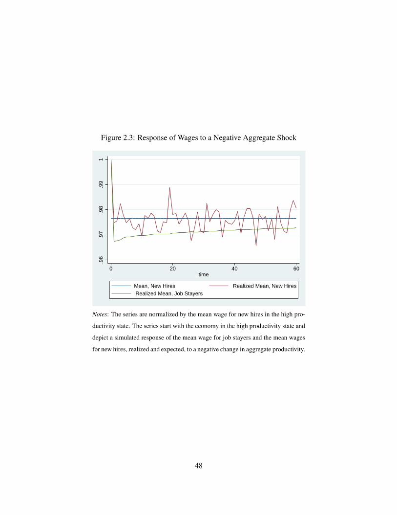
I outline a mechanism that explains how the wages of new hires can be less procyclical than for

job stayers due to the cyclical properties of the average match-specific productivity for two groups.

The wages are determined by Nash bargaining over the match surplus, which depends on aggregate

productivity and match-specific productivity. The average match-specific productivity moves in

1As discussed later, the presence of a firing cost has the same effect.

25

the opposite direction to aggregate productivity for both job stayers and new hires, which affects

the wages countercyclically. The presence of turnover costs drives a wedge between the lowest

viable match-specific productivity for new hires and job stayers, making changes in the average

match-specific productivity more pronounced for new hires. As a result, the average match-specific

productivity for new hires is countercyclical in both absolute terms and relative to job stayers,

which dampens procyclicality of the wages of new hires relative to the wages of job stayers.

The presence of low productivity matches that can be created only when productivity is high

drives a positive relationship between initial aggregate productivity and the subsequent risk of

separation, which translates into the negative relationship between the initial unemployment rate

and the separation risk. The low productivity matches undergo an endogenous separation when

aggregate productivity drops.

When aggregate productivity is high, even matches with low match-specific productivity are

productive enough to cover a hiring cost. The matches for job stayers are a mixture of matches

that survived previous periods of low aggregate productivity and matches created in recent periods

of high productivity. Consequently, the distribution of match-specific productivity of job stayers

stochastically dominates the distribution of match-specific productivity of new hires.

When aggregate productivity is low, the matches of new hires have high match-specific pro-

ductivity, because only such matches are productive enough to cover a hiring cost. The previously

created matches with low match-specific productivity are destroyed. The existing matches with

medium and high match-specific productivity are productive enough to survive, even though some

of them are not productive enough to cover a hiring cost. The matches of job stayers are a mix-

ture of matches created in previous periods which are productive enough to survive, and matches

created in recent periods of low productivity. Consequently, the distribution of match-specific pro-

ductivity of new hires stochastically dominates the distribution of match-specific productivity of

26

job stayers.

I calibrate the model using external sources to inform the value of a hiring cost and the dis-

tribution of match-specific productivity. I compare the cyclical properties of the model-generated

wages and the observed wages, and the properties of job duration for generated job spells and

the observed spells. The model-generated wages have similar cyclical properties as the observed

wages: the wages of new hires are less procyclical than the wages of job stayers. Matches created

when aggregate productivity are at a decreased risk of subsequent separation.

2.2 Related Literature

The key elements of the model I use are match-specific productivity and turnover costs. Both

features appeared in the previous literature. However, their interaction and consequences for the

cyclical properties of wages were unexplored.

2.2.1 Match-Specific Productivity

The match quality defined as the idiosyncratic productivity of a worker-firm pairing was popular-

ized by Jovanovic (1979 a,b; 1984). In the Jovanovic learning model, the match quality is a pure

experience good: it is assigned randomly when a job is created and its value is revealed over tenure

by observed output. Moscarini (2005) embeds this idea into the Diamond-Mortensen-Pissarides

search and matching model, with the match quality taking only one of two values. The conse-

quences for wages in a steady state are considered: the selection on match quality moves workers

to matches with higher perceived quality and higher wages, giving the wage distribution a long and

fat right tail, which is observed empirically.

Pries and Rogerson (2005) combine a variant of the Jovanovic learning model, in which the

27

match quality is partially an inspection and partexperience good, and the Diamond-Mortensen-

Pissarides search and matching model to investigate the steady state effects of, among others,

turnover costs in the form of dismissal costs. In this variant of the learning model, a firm and a

worker receive a signal before a match is formed, giving them a probability of the match being bad

or good. The match quality is then revealed gradually by output observations. Similarly to this

paper, the higher dissmisal costs push up the threshold for the signal about match quality above

which matches are accepted.

More generally, the standard assumption in the search and matching literature is that new

matches start with the same match-specific productivity, which later evolves, as in Mortensen

and Pissarides (1994), Pissarides (2009), and Fuijta and Ramey (2012). Matches were allowed to

start with randomly drawn productivity in Mortensen (1982) and Mortensen and Nagypal (2007b).

However, the consequences of the presence of match-specific productivity for the cyclical proper-

ties of wages were not investigated.

A paper closely related to mine is Gertler, Huckfeldt and Trigari (2016). They build a model

with match-specific productivity, which takes two values, and endogenous on-the-job search. The

model generates a procyclical selection effect for new hires from employment. An interesting im-

plication is that jobs created by a job-to-job transition during downturns should be at an increased

risk of ending with a subsequent job-to-job transition. The implication was not investigated in the

paper.

The consequences of match quality selection for wages appear in a different context in Hage-

dorn and Manovskii (2013). They argue that when wages depend on current conditions and match-

specific productivity, past selection over match quality makes wages appear to depend on past

labor market conditions summarized by the lowest unemployment rate during a job spell. Their

preferred proxies for match quality are derived from measures of labor market tightness during a

28

job spell and an employment cycle. In future empirical work, I plan to use information on past

and future labor market conditions to control for match quality in the estimation of cyclicality of

wages, along the lines of Beaudry and DiNardo (1991) and Hagedorn and Manovskii (2013), but

with a focus on the most adverse labor market conditions which a job survives.

2.2.2 Turnover Costs

Turnover (hiring or firing) costs were added to the search and matching model in Braun (2006),

Nagypal (2007), Silva and Toledo (2009) and Yashiv (2006). Turnover costs improve the perfor-

mance of the model by making firms’ net profits more responsive to changes in productivity.

Muehlemann and Pfeifer (2016) use a German firm-level survey from the 2000s to assess the

recruitment and adaptation costs generated by job creation. The average total hiring cost in Ger-

many was equal to more than 2 months of wage payments, with two-thirds of this cost incurred

when a worker was hired, and one-third generated by vacancy creation and screening of applica-

tions. I use the provided ratio of a hiring cost to wages in my model calibration. For the US, Dube

et al. (2010) assess the average total hiring cost to be approximately 1.1 of the monthly wages in

California, which suggests that the hiring cost should be twice as high in Germany as in the US.

A characteristic feature of the German labor market is that the firing costs are high. Unlike in

the US, an employee with a permanent contract that is dismissed on operational grounds is entitled

to severance pay equal to half of a monthly wage for each year of tenure, up to 12 monthly wages

for most workers, and even more for older workers with long tenure.

29

2.3 Selection Effect: Stylized Example

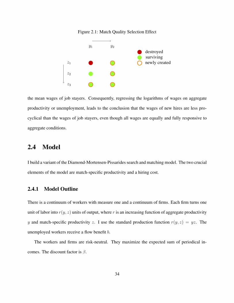
In this section, I use a stylized example to illustrate the mechanism generating the cyclical prop-

erties of wages and job duration. Aggregate productivity takes two values, low y1 and high y2;

match-specific productivity has three values z1, z2, and z3, such that z1 < z2 < z3; and agents are

myopic, discounting with factor 0. I leave vacancy creation decision unspecified, assuming only

that vacancies are created in both aggregate states, and that there are no more vacancies created in

the low productivity state than in the high productivity state.

A worker in a match with match-specific productivity z produces zy when aggregate produc-

tivity is y, receiving a fraction τ of his output. His employer receives (1− τ)zy. The worker quits

if his wage τzy is lower than the unemployment benefit b.2 The probability that an exogenous

separation occurs is δ.

When an unemployed worker and a vacancy-posting firm meet, they draw value z of match-

specific productivity from a fixed distribution. The firm has to incur a sunk cost h, but only if a

job is created. The firm wants to create a job if its per-period earnings would cover the hiring cost,

(1 − τ)zy ≥ h. The worker wants the job if his wage would be no less than the unemployment

benefit, τzy ≥ b.

Figure 1 summarizes the model under parameter values ensuring that the match quality selec-

tion effect is present. The parameters have to satisfy the inequalities

z3 ≥h

(1− τ)y1

> z2 ≥b

τy1

> z1 ≥h

(1− τ)y2

(2.1)

which is possible. When aggregate productivity is high, all possible matches produce enough

output to be preferable to unemployment for workers and to justify job creation for firms. There are

2For clarity of exposition, I assume that a firm and a worker split the match output zy, not the surplus zy − b. Thereasoning goes through when they split the surplus instead.

30

no endogenous separations. When aggregate productivity is low, the lowest-productivity matches

are destroyed, because workers find unemployment preferable. The medium-productivity matches

are preferable to unemployment for workers, but are not productive enough to cover the hiring cost,

which means that the existing medium-productivity matches survive but there no new medium-

productivity matches.

In the low productivity state, there are no less separations than in the high state - endogenous

separations happen only in the first period after a drop in aggregate productivity, and the rate of

exogenous separations is constant. Under the assumption that vacancy creation does not increase

in the low productivity state, and taking into account that some worker-firm meetings in the low

state do not lead to match creation due to drawing low match-specific productivity, there is less job

creation when aggregate productivity is low. Consequently, the unemployment rate rises in the low

productivity state.

Because unemployment is higher when aggregate productivity is lower, the relationships be-

tween the model outcomes, the wages and job durations, and aggregate productivity translate into

the relationships between the model outcomes and the unemployment rate. I show that the wages

and job durations generated in a model that satisfies the condition (2.1) have the desired cyclical

properties.

The relationship between the initial unemployment rate and the subsequent risk of separation is

negative. The risk of exegenous separation is constant and independent of initial conditions. Only

endogenous separations are those of workers that quit low-productivity matches when aggregate

productivity is low.

I proceed to show that the wages of new hires are less procyclical than the wages of job stayers.

The cyclical properties of wages result from the properties of the distributions of match-specific

productivity for new hires and job stayers. The distribution of match-specific productivity for new

31

hires stochastically dominates the distribution of match-specific productivity for job stayers when

aggregate productivity is low, but the reverse happens when aggregate productivity is high.

The distribution of match-specific productivity for new hires is the same as the underlying

distribution of match-specific productivities when aggregate productivity is high. When aggregate

productivity is low, all match-specific productivities of new hires are equal to z3. Consequently,

the mean wages of new hires are wH2 = τy2Ez and wH1 = τy1z3, in upturns and in downturns,

respectively.

When aggregate productivity is high, job stayers belong to one of three groups: workers that

were hired during the current upturn, with the same match-specific productivity distribution as

the underlying distribution of match-specific productivities, which mean is Ez; workers that were

hired during a previous upturn and remained employed during a downturn, with a match-specific

productivity distribution that is a truncation of the underlying distribution of match-specific pro-

ductivities without z1, which mean is Ez|z > z1; and workers that were hired during a previous

downturn, who are employed exclusively in matches with productivity z3. Let the fractions of the

second and third group of workers in the total number of employed workers be π and π′.

The distribution of match-specific productivity for job stayers during upturns is a mixture of

three distributions. Two of these distributions stochastically dominate the match-specific produc-

tivity distribution for new hires, one of them is the same distribution. Consequently, the distribution

of match-specific productivity for job stayers stochastically dominates the distribution of match-

specific productivity for new hires.

The mean wage of job stayers is

wS2 (π, π′) = (1− π − π′)τy2Ez + πτy2Ez|z > z1 + π′τy2z3

where π, π′ ∈ [0, 1], such that π + π′ ∈ [0, 1], depend on the rate of exegenous separations, and

32

history of vacancy creation and of aggregate states. The mean wage of job stayers, wS2 (π, π′), is

higher than the mean wage of new hires, wH2 = τy2Ez, as long as π + π′ < 1.

When aggregate productivity is low, job stayers belong to one of two groups: workers that were

hired during the current or a previous downturn, who are employed exclusively in matches with

productivity z3; or workers that were hired during a previous upturn and remain employed during

a downturn, with a match-specific productivity distribution that is a truncation of the underlying

distribution of match-specific productivities without z1, which mean is Ez|z > z1. Let the fraction

of the second group of workers in the total number of employed workers be γ.

The distribution of match-specific productivity for job stayers during downturns is a mixture

of 3 distributions. One of these distributions is stochastically dominated by the match-specific

productivity distribution for new hires, the other two are the same distribution. Consequently, the

distribution of match-specific productivity for new hires stochastically dominates the distribution

of match-specific productivity for job stayers.

The mean wage of job stayers is

wS1 (γ) = (1− γ)τy1z3 + γτy1Ez|z > z1

where γ ∈ [0, 1] depends on the rate of exegenous separations, and history of vacancy creation and

of aggregate states. The mean wage of job stayers, wS1 (γ), is lower than the mean wage of new

hires, wH1 = τy1z3, as long as γ > 0.

The inequalities wS1 (γ) < wH1 and wH2 < wS2 (π, π′) imply that

wS1 (γ)− wS2 (π, π′)

wS2 (π, π′)<wH1 − wH2

wH2,wH2 − wH1

wH1<wS2 (π, π′)− wS1 (γ)

wS1 (γ). (2.2)

When wH1 < wh2 , which is guaranteed by assuming that y1z3 < y2Ez, inequalities (2.2) show

that, in percentage terms, the mean wages of new hires respond less to aggregate productivity than

33

Figure 2.1: Match Quality Selection Effect

z3

z2

z1

y1 y2

destroyedsurvivingnewly created

the mean wages of job stayers. Consequently, regressing the logarithms of wages on aggregate

productivity or unemployment, leads to the conclusion that the wages of new hires are less pro-

cyclical than the wages of job stayers, even though all wages are equally and fully responsive to

aggregate conditions.

2.4 Model

I build a variant of the Diamond-Mortensen-Pissarides search and matching model. The two crucial

elements of the model are match-specific productivity and a hiring cost.

2.4.1 Model Outline

There is a continuum of workers with measure one and a continuum of firms. Each firm turns one

unit of labor into r(y, z) units of output, where r is an increasing function of aggregate productivity

y and match-specific productivity z. I use the standard production function r(y, z) = yz. The

unemployed workers receive a flow benefit b.

The workers and firms are risk-neutral. They maximize the expected sum of periodical in-

comes. The discount factor is β.

34

The aggregate productivity, y, is the same for all firms, with values in the set Y = {y1, y2, .., yNY },

where y1 < y2 < ... < yNY and NY ≥ 2. The aggregate productivity y is updated to y at the be-

ginning of the next period with probability fY (y, y), where fY : Y 2 → [0, 1].

The match-specific productivity, z, with values in the setZ = {z1, z2, .., zNZ}, where z1 < z2 <

... < zNZ and NZ ≥ 2, is fixed for each match after being drawn from a probability distribution

with a cumulative distribution function FZ . The match-specific productivity is drawn when a

worker and a firm meet, but before a worker is hired.

The notation for value functions is standard. The value of match to the firm, the value of match

to the worker, the value of unemployment to the worker, and the match surplus are denoted as

J(y, z), W (y, z), U(y), and S(y, z) = J(y, z) +W (y, z)− U(y).

The Nash bargaining divides the match surplus. The contract between a firm and its employee

specifies the wagew(y, z). The wage equalizes the worker’s surplusW (y, z)−U(y) with τS(y, z),

where τ ∈ [0, 1] is the workers’ bargaining power parameter.

There is a hiring cost h ≥ 0 that has to paid in the first period of employment. This is a sunk

cost that is incurred only if a job is created and that does not enter into the match surplus.

The firms create vacancies which meet workers through a frictional meeting process. The

number of meetings is determined by a CRS matching function M(u, v), which depends on the

mass of created vacancies, v, and the mass of workers looking for jobs, u. The probabilities that the

workers and vacancies meet is M(u, v)/u for workers and M(u, v)/v for the vacancies, which can

be written as functions of labor market tightness θ = v/u. An unemployed worker meets a vacancy

with probability p(θ) = M(1, θ), a vacancy meets a worker with probability q(θ) = M(θ−1, 1).

The zero profit condition determines vacancy creation. The firms’ expected profit from vacancy

creation depends on the probability of meeting a worker and the expected value of meeting a

worker, denoted as J(y). If the expected value exceeds the cost of vacancy creation, c > 0,

35

vacancies are created until the expected profit is driven to zero. If the expected value is less than

the cost of vacancy creation, no vacancies are created. Labor market tightness is determined in the

equilibrium as

θ(y) =

q−1(c/J(y)), if J(y) ≥ c

0. if J(y) < c.

(2.3)

Matches are destroyed if the surplus S(y, z) is negative and with the exogenous separation

probability δ ∈ (0, 1). For simplicity, I assume that the workers who lose a job cannot find a new

one in the same period.

2.4.2 Value Functions

The match surplus S is a sum of the firm’s surplus, J , and the worker’s surplus, W −U , where W

and U are the value of employment and unemployment. The Nash bargaining leads to the condition

J(y, z)

1− τ= S(y, z) =

W (y, z)− U(y, z)

τ.

The value accruing to an unemployed worker is

U(y) =b+ βE[(

1− p(θ(y)))U(y)

+ p(θ(y))

∫1{(1− τ)S(y, z) < h}dFZ(z)U(y)

+ p(θ(y))

∫1{(1− τ)S(y, z) ≥ h}W (y, z)dFZ(z)

]which can be rewritten as

U(y) =b+ βE[U(y) + p(θ(y))

∫1{(1− τ)S(y, z) ≥ h}τS(y, z)dFZ(z)

].

The value accruing to an employed worker is

W (y, z) =w(y, z) + βE[δU(y)

+ (1− δ)1{S(y, z) < 0}U(y)

+ (1− δ)1{S(y, z) ≥ 0}W (y, z)]

36

which can be rewritten as

W (y, z) =w(y, z) + βE[U(y) + (1− δ)1{S(y, z) ≥ 0}τS(y, z)

].

The value accruing to a firm employing a job stayer is

J(y, z) =r(y, z)− w(y, z) + βE(1− δ)1{S(y, z) ≥ 0}J(y, z)

which can be rewritten as

J(y, z) =r(y, z)− w(y, z) + βE(1− δ)1{S(y, z) ≥ 0}(1− τ)S(y, z).

The surplus S can be rewritten as

S(y, z) =r(y, z)− b+ βE[(1− δ)1{S(y, z) ≥ 0}S(y, z)−

p(θ(y))

∫1{(1− τ)S(y, z) ≥ h}τS(y, z)dFZ(z)

].

(2.4)

The expected value of meeting a worker is

J(y) =

∫1{(1− τ)S(y, z) ≥ h}((1− τ)S(y, z)− h)dFZ(z). (2.5)

2.4.3 Equilibrium

The equations (2.3)-(2.5) define a functional operator. An equilibrium is a surplus function S

satisfying the equation (2.4), where a market tigthness function θ is dictated by the equations (2.5)

and (2.3). The equilibrium is a fixed point of a functional operator.

The equilibrium operator is not continuous, which is the the only obstacle that precludes prov-

ing the equilibrium existence with the use of the Brouwer’s fixed-point theorem.3 I consider a

3The standard method of proving the equilibrium existence and uniqueness by proving that the equilibrium operatorsatisfies Blackwell’s sufficient conditions, as in Mortensen and Nagypal (2007b), is not applicable, because terms ofthe type 1{x ≥ 0}x introduce non-convexity.

37

proxy of the model. In the proxy model, the equilibrium operator is continuous. I prove the equi-

librium existence for the proxy model in Appendix A. If, in the equilibrium, the proxy model

reduces to the original model, then the equilibrium of the proxy model is also an equilibrium of the

original model. The discontinuity of the equlibrium operator stems from the presence of a hiring

cost that is excluded from the match surplus. The existence of an equilibrium in a model in which

a hiring cost enters the match surplus can be proved directly.

I use the Brouwer’s theorem, which does not guarantee the equilibrium uniqueness and is not

constructive. However, I take the advantage of the properties of the equilibrium operator, which can

be decomposed in a sum of its increasing and decreasing parts. I adopt a method that numerically

narrows the space of potential equilibria, which I discuss in Appendix B.

2.4.4 Match Creation and Match Survival Thresholds

When aggregate productivity is y, a match with match-specific productivity z is not endogenously

destroyed if the condition S(y, z) ≥ 0 is satisfied, and can be created if the condition S(y, z) ≥

h is satisfied. When S(y, z) is increasing in the second argument, z, there are match-specific

productivity thresholds for match survival and match creation,

zs(y) = minz∈Z{S(y, z) ≥ 0}

and

zc(y) = minz∈Z{S(y, z) ≥ h},

with the following properties: z > zs(y) implies that S(y, z) ≥ 0 and a match with match-specific

productivity z is not endogenously destroyed; z > zc(y) implies that S(y, z) ≥ h and a match with

match-specific productivity z can be created; and zc(y) ≤ zs(y), the threshold for match creation

38

is more demanding than for match survival. When S(y, z) is also increasing in the first argument,

y, the thresholds are non-increasing functions of aggregate productivity, y.

For the highest aggregate productivity, yNY , it can be assumed without loss of generality that

the thresholds for match survival and match creation coincide, zc(yNY ) = zs(yNY ) = z1, which

together with zs(y) ≤ zc(y) implies that

zc(yNY ) = zs(yNY ) ≤ zc(y) ≤ zs(y) (2.6)

for any aggregate productivity y.

2.4.5 Match-Specific Productivity for New Hires and Job Stayers

To illustrate the selection effect it is sufficient to consider two aggregate productivity states, low

y1 and high y2. In this section, I show that the selection effect is present if there are some matches

that can survive but cannot be created when aggregate productivity is low, zs(y1) < zc(y1), which

together with (2.6) implies that

zs(y1) < zc(y1) ≤ zc(y2) = zs(y2). (2.7)

There are four groups of workers whose match-specific productivity distributions I consider,

new hires and job stayers when aggregate productivity is low and when aggregate productivity is

high.

A match-specific productivity distribution for new hires, H(z; y), is a truncation of the un-

derlying match-specific productivity distribution, F , that restricts its domain to match-specific

productivities that are above the match creation threshold

H(z; y) =F (z)

1− F (zc(y)).

For high aggregate productivity, y2, the distributions H(z; y) and F (z) coincide.

39

The inequalities (2.7) guarantee that there are some matches that can survive but cannot be

created when aggregate productivity is low. The match-specific productivity distribution for such

matches is

P (z) =F (z)

1− F (zs(y1)).

When aggregate productivity is low, job stayers belong to one of two groups: workers that were

hired during the current or a previous episode of low productivity, whose match-specific produc-

tivity distribution is H(z; y1); or workers that were hired during an episode of high productivity

and remain employed during a downturn, whose match-specific productivity distribution is P (z).

The match-specific productivity distribution for job stayers is

G(z; y1, γ) = (1− γ)H(z, y1) + γP (z)

where γ ∈ [0, 1], the fraction of the second group of workers, decreases in the duration of low-

productivity episode.

When aggregate productivity is high, job stayers belong to one of three groups: workers that

were hired during the current episode of high productivity, whose match-specific productivity dis-

tribution is H(z; y2); workers that were hired during a previous episode of high productivity and

remained employed during a previous episode of low productivity, whose match-specific produc-

tivity distribution is P (z); or workers that were hired during a previous episode of low productivity,

whose match-specific productivity distribution is H(z; y1). The match-specific productivity distri-

bution for job stayers is

G(z, y2, π, π′) = (1− π − π′)H(z, y2) + πP (z) + π′H(z, y1)

where the fractions of the second and third group of workers are π and π′, which decrease in the

duration of high-productivity episode.

40

The inequalities (2.7) imply that the match-specific productivity distributions can be ordered

the sense of first-order stochastic dominance. The ordering H(z; y2), P (z) ≺ H(z; y1) implies the

ordering

H(z; y2) ≺ G(z, y2, π, π′), G(z; y1, γ) ≺ H(z; y1). (2.8)

The first-order stochastic dominance ordering (2.8) implies inequalities between the means

of the four distributions. The mean match-specific productivity for new hires when aggregate

productivity is high is the lowest of the four means, the mean match-specific productivity for new

hires when aggregate productivity is low is the of the four means, and the means for job stayers lie

between these two extremes. When the means ofH(z; y2),G(z, y2, π, π′),G(z; y1, γ) andH(z; y1)

are denoted as zH2 , zS2 (π, π′), zS1 (γ) and zH1 , the inequalities between the means are

zH2 < zS2 (π, π′), zS1 (γ) < zH1 (2.9)

The inequalities (2.9) lead to a conclusion that the mean match-specific productivity for new

hires is countercyclical, rising when aggregate productivity is lower, and that its cyclical changes

are smaller than the cyclical changes in the mean match-specific productivity for job stayers.

2.4.6 Calibration

The calibration is at a monthly frequency. The model has 11 parameters, summarized in Table 2.1.

For 4 parameters I use paremeters values that are common in the literature. I calibrate 7 remaining

parameters using external information.

41

Table 2.1: Model Parameters

Value Description Target/Source

h = 1.9 hiring cost Muehlemann and Pfeifer (2016)

σ = 0.3 sd of log match productivity Card, Heining, and Kline (2013)

β = 0.9966 discount factor standard, annual interest rate 4.17%

η = 0.5 matching function elasticity standard, Pissarides and Petrongolo (2001)

τ = 0.5 workers’ bargaining power standard, Hosios’ condition, τ = η

σy = 0.02 aggregate productivity sd standard, Shimer (2005)

ρ = 1/24 transition probabilities standard, 2-year long recessions

δ = 0.0095 exogenous separation rate separations, Elsby et al. (2013), Nordmeier (2014)

b = 0.55 unemployment benefit Krause and Uhlig (2012)

c = 0.42 vacancy creation cost un, job finding, Elsby et al. (2013), Nordmeier (2014)

κ = 0.35 matching efficiency un, job finding, Elsby et al. (2013), Nordmeier (2014)

The key features of the model are a hiring cost and match-specific productivity. I use external

sources to inform the value of the hiring cost and the match-specific productivity distribution.

The hiring cost h is calibrated to be approximately 1.3 of the mean monthly wage, as calculated

by Muehlemann and Pfeifer (2016) from a survey of German firms.

I follow the literature and assume that match-specific productivity has a lognormal distribution

with a standard deviation σ. The data moment used to calibrate σ is the standard deviation of

the residual log wages, taken from Card, Heining, and Kline (2013), who estimated the Mincer

equation for log wages using the whole universe of German labor market biographies.

The parameters β, η, τ and ρ have values standard in the literature. The aggregate productivity

is either low, 1 − σy, or high, 1 + σy. Tha parameter σy targets the standard deviation 0.02 of log

labor productivity, as in Shimer (2005).

The exogenous separation rate δ = 0.095 is equal to the lower values of the monthly separation

rate in the 2000s calculated in Nordmeier (2014) and consistent with previous calculations in Elsby

42

et al. (2013).

The unemployment benefit b is calibrated to target 0.4 of mean monthly labor income, as in

Krause and Uhlig (2012) for the post-Hartz period.

I use the standard matching function M(u, v) = κuηv(1−η).4. The vacancy creation cost c and

the matching function efficiency parameter κ are jointly calibrated to match the mean monthly job

finding rate calculated in Nordmeier (2014) and Elsby et al. (2013), around 0.055− 0.07, and the

mean monthly unemployment rate 0.09.

The model outcomes, summarized and compared with target moments in Table 2.2, are gen-

erated from simulations of the model with 2400 monthly observations on 10000 workers with 51

possible match-specific productivities.

Table 2.2: Model Fit

Outcome Target Description

1.29 1.3 hiring cost relative to w

0.11 0.14 sd of (residual) log wages

0.37 0.4 unemployment benefit relative to w

0.12 0.09 unemployment rate

0.01 0.01 separation rate

0.07 0.055-0.07 job finding rate

Notes: w denotes mean labor income.

2.4.7 Properties of Model-Generated Data

The first empirical finding of the previous chapter is that the wages of new hires are less procyclical

than the wages of job stayers. To confirm that this cyclical property arises in the model, I estimate

4The function has to be truncated by the condition M(u, v) ≤ min{u, v}, which is equivalent to a restriction θ ∈[κ1/η, κ1/(1−η)]

43

the wage equation

log wit = πut + πUNHU(i, t)ut + γNHU + εit (2.10)

where wit is the wage paid in period t in match i, ut is the unemployment rate, and NHU(i, t) is

an indicator variable that takes value one for new hires, using simulated wages.

Table 2.3 shows the averaged estimates from Equation 2.10. The wages have the key cyclical

property matching the empirical findings from the previous chapter: the estimated incremental

effect πU = 0.46 is positive and significant, and of similar magnitude as the analogous estimate in

the previous chapter. For all simulations, the estimates are significant and have the desired cyclical

properties.

Table 2.3: Wage Cyclicality Estimates for Model-Generated Wages

π −1.85

πU 0.46

Notes: Average values from 5 simulations of 2400 monthly observa-

tions on 20000 workers with 51 possible match-specific productivities.

To complete the analysis of cyclical properties of wages, I solve and simulate the model with-

out a hiring cost, setting h = 0. Table 2.4 shows averages of estimates of Equation 2.10 for

simulated wages. The baseline estimate of wage cyclicality, π, decreases from −1.85 to −2.54.

The incremental effect for wages of new hires, πU , is small and insignificant in all simulations.

The differences between the cyclical properties for the model with and without a hiring cost

are expected. The thresholds for match creation and match maintenance coincide in this model,

which implies the wages of job stayers and new hires have the same cyclicality. In the model with

a hiring cost, when aggregate productivity is low, a fraction of job stayers are workers that were

44

hired during the current episode of low productivity, whose match-specific productivity undergoes

the strongest selection, which decreases the cyclicality of wages of job stayers.

Table 2.4: Wage Cyclicality Estimates for Model-Generated Wages, No Hiring Cost

π −2.54

πU 0.09

Notes: Average values from 5 simulations of 2400 monthly observa-

tions on 20000 workers with 51 possible match-specific productivities.

The second empirical finding of the previous chapter is that unemployment at the beginning

of employment and the subsequent risk of separation are negatively related. For comparison with

model outcomes, I estimate the Cox (1972) model using simulated unemployment and job dura-

tions. The hazard rate hid for match i after d periods from hiring takes the functional form

hid = hdexp(αustarti + εid) (2.11)

where hd is the baseline hazard rate common to all matches and ustarti is the unemployment rate at

the creation of match i. Table 2.5 shows averages of estimates of Equation 2.11.

Table 2.5: Estimates for Job Duration

α −0.61

Notes: Average values from 5 simulations of 2400 monthly observa-

tions on 20000 workers with 51 possible match-specific productivities.

Finally, I illustrate the responses of wages to productivity changes: Figure 2.2 shows the simu-

lated response of mean wages to a positive shock to aggregate productivity, and Figure 2.3 shows

the simulated response of mean wages to a negative shock to aggregate productivity.

45

As seen in Figure 2.2, after the shock the mean wages of job stayers and new hires increase. The

mean wages wages of job stayers are higher than for new hires, due to the presence of workers that

were survived or were hired during previous episodes of low productivity, and gradually decrease

to the mean wages of new hires as the share of workers hired during the current episode of high

productivity.

Conversely, as Figure 2.3 shows, after the shock the mean wages of job stayers and new hires

decrease. The mean wages wages of job stayers are lower than for new hires, due to the presence

of workers that were hired during previous episodes of high productivity, and gradually increase

to the mean wages of new hires as the share of workers hired during the current episode of low

productivity.

46

Figure 2.2: Response of Wages to a Positive Aggregate Shock

11.

011.

021.

031.

04

0 20 40 60time

Mean, New Hires Realized Mean, New Hires Realized Mean, Job Stayers

Notes: The series are normalized by the mean wage for new hires in the low pro-

ductivity state. The series start with the economy in the low productivity state and

depict a simulated response of the mean wage for job stayers and the mean wages

for new hires, realized and expected, to a positive change in aggregate productivity.

47

Figure 2.3: Response of Wages to a Negative Aggregate Shock

.96

.97

.98

.99

1

0 20 40 60time

Mean, New Hires Realized Mean, New Hires Realized Mean, Job Stayers

Notes: The series are normalized by the mean wage for new hires in the high pro-

ductivity state. The series start with the economy in the high productivity state and

depict a simulated response of the mean wage for job stayers and the mean wages

for new hires, realized and expected, to a negative change in aggregate productivity.

48

2.5 Conclusions

The match quality selection effect arises in a standard Diamond-Mortensen-Pissarides search and

matching model with two additional features: match-specific productivity and turnover costs. The

cyclical selection on match quality explains the empirical findings of the previous chapter, the

wages of new hires being less procyclical than the wages of job stayers, and a negative relationship

between the initial unemployment rate and the subsequent risk of separation.

More generally, these two fairly realistic features could generate the same selection effect in

models with different wage-setting mechanisms. An example would be a model with staggered

multiperiod Nash bargaining in which workers’ wages are negotiated for the first time when they

are hired.5 Without the selection effect, the wages of new hires would be more procyclical than

the wages of job stayers, which are not fully flexible. With the selection effect induced by match-

specific productivities and turnover costs, the observed procyclicality of the wages of new hires

relative to job stayers would be attenuated. The estimation of the cyclicality of model-generated

wages could lead to an incorrect conclusion that the wages of new hires were no more or not much

more procyclical than the wages of job stayers.

The empirical results of the previous chapter suggest that the match quality selection effect

is stronger for hires from employment than from unemployment. The on-the-job search can be

incorporated into the model to account for job-to-job transitions. In the present form, the model

would not generate the stronger selection effect for hires from employment than for hires from un-

employment. However, a conceptually easy modification should resolve this issue. For simplicity,

I made match-specific productivity an inspection good, known to workers and firms immediately

upon meeting. I could relax this assumption, making match-specific productivity partially an ex-

5Unlike Gertler and Trigari (2009), where workers hired in-between wage renegotiations receive the ongoing wage.

49

perience good. Then, worker-firm pairs receive a signal about match-specific productivity upon

meeting. If they agree to form a match, the underlying productivity is revealed during first few

months of its duration.6 For hires from unemployment, the same force driving the selection effect

in the baseline model appears in the generalized model. For hires from employment, the selection

effect is enhanced: during downturns, the employed workers are concerned about a risk of job loss

in a new match, since unemployment spells are longer in expectation, and demand a higher signal

about match quality to accept an offer of a job-job transition.

6This is consistent with the observation that risk of separation is elevated during first few months on job, and goesdown sharply afterwards.

50

Bibliography

[1] Barlevy, Gaudi. 2002. ”The Sullying Effect of Recessions.” Review of Economic Studies

69(1), 65-96.

[2] Beaudry, Paul, and John DiNardo. 1991. ”The Effect of Implicit Contracts on the Movement

of Wages over the Business Cycle: Evidence from Micro Data.” Journal of Political Economy

99(4): 665-88.

[3] Braun, Helge. 2006. ”(Un)Employment Dynamics: The Case of Monetary Policy Shocks.”

Society for Economic Dynamics Meeting Papers 87.

[4] Collatz, Lothar. 1966. ”Functional analysis and numerical mathematics.” New York: Aca-

demic Press.

[5] Dube, Arindrajit, Eric Freeman, and Michael Reich. 2010. ”Employee Replacement Costs.”

Working Paper Series, Institute of Industrial Relations, UC Berkeley.

[6] Jovanovic, Boyan. 1979a. “Job Matching and the Theory of Turnover.” Journal of Political

Economy 87(5): 972-90.

[7] Jovanovic, Boyan. 1979b. “Firm-Specific Capital and Turnover.” Journal of Political Econ-

omy 87(6): 1246-60.

51

[8] Jovanovic, Boyan. 1984. “Matching, Turnover, and Unemployment.” Journal of Political

Economy 92(1): 108-22.

[9] Gertler, Mark, Christopher Huckfeldt, and Antonella Trigari. 2016. ”Unemployment Fluctua-

tions, Match Quality, and the Wage Cyclicality of New Hires.” National Bureau of Economic

Research Working Paper 22341.

[10] Gertler, Mark, and Antonella Trigari. 2009. ”Unemployment Fluctuations with Staggered

Nash Wage Bargaining.” Journal of Political Economy 117(1): 38-86.

[11] Hagedorn, Marcus, and Iourii Manovskii. 2013. ”Job Selection and Wages over the Business

Cycle.” American Economic Review 103(2): 771-803.

[12] Hall, Robert. 2005. ”Job Loss, Job Finding, and Unemployment in the U.S. Economy over

the Past Fifty Years.” NBER Macroeconomics Annual 20: 101-137.

[13] Krause, Michael, and Harald Uhlig. 2012. ”Transitions in the German labor market: Structure

and crisis.” Journal of Monetary Economics 59(1): 64-79.

[14] Krause, Michael, and Harald Uhlig. 2012. ”Transitions in the German labor market: Structure

and crisis.” Journal of Monetary Economics 59(1): 64-79.

[15] Mortensen, Dale. 1982. ”The Matching Process as a Noncooperative Bargaining Game.”

In Economics of Information and Uncertainty, edited by John J. McCall, 233-258. Chicago:

University of Chicago Press.

[16] Mortensen, Dale, and Eva Nagypal. 2007a. ”Labor-market Volatility in Matching Models

with Endogenous Separations.” Scandinavian Journal of Economics 109(4): 645-665.

52

[17] Mortensen, Dale, and Eva Nagypal. 2007b. ”More on Unemployment and Vacancy Fluctua-

tions.” Review of Economic Dynamics 10(3): 327-347.

[18] Mortensen, Dale, and Christopher Pissarides. 1994. ”Job Creation and Job Destruction in the

Theory of Unemployment.” Review of Economic Studies 61(3): 397-415.

[19] Nagypal, Eva. 2007. ”Labor-Market Fluctuations and On-the-Job Search.” Unpublished.

[20] Pissarides, Christopher. 2000. ”Equilibrium Unemployment Theory.” Cambridge, MA: MIT

Press.

[21] Pissarides, Christopher. 2009. ”The Unemployment Volatility Puzzle: Is Wage Stickiness the

Answer?” Econometrica 77(5): 1339-1369.

[22] Pissarides, Christopher, and Barbara Petrongolo. 2001. ”Looking into the Black Box: A

Survey of the Matching Function” Journal of Economic Literature 39(2): 390-431.

[23] Pries, Michael, and Richard Rogerson. 2005. ”Hiring Policies, Labor Market Institutions,

and Labor Market Flows.” Journal of Political Economy 113(4): 811-839.

[24] Silva, Jose, and Manuel Toledo. 2009. ”Labor Turnover Costs and the Behavior of Vacancies

and Unemployment” Macroeconomic Dynamics 13(1): 76-96.

[25] Yashiv, Eran. 2006. ”Evaluating the performance of the search and matching model.” Euro-

pean Economic Review 50(4): 909-936.

53

Appendix A: Equilibrium Existence

The equilibrium operator, denoted as T , is defined by the equations (2.3)-(2.5). I use notation

P (y) = p(θ(y)) for the composite vacancy-meeting probability, and subscript S for the depen-

dence on S, writing T as

T S(y, z) =r(y, z)− b+ βE[(1− δ)1{S(y, z) ≥ 0}S(y, z)−

P S(y)

∫1{(1− τ)S(y, z) ≥ h}τS(y, z)dFZ(z)

],

where

θS(y) =

q−1(c/JS(y)), if J(y) ≥ c

0. if J(y) < c

and

JS(y) =

∫1{(1− τ)S(y, z) ≥ h}((1− τ)S(y, z)− h)dFZ(z).

The operator T is not continuous. There are at most two sources of discontinuity: the compo-

nents 1{(1− τ)S(y, z) ≥ h}τS(y, z) and, potentially, the vacancy-meeting probability P S(y).7

In the proxy model, I replace the indicator function 1{(1 − τ)S(y, z) ≥ h} by a function

defined as

aS(y, z) =

0, if (1− τ)S(y, z)− h ≤ 0

1d

((1− τ)S(y, z)− h

), if 0 ≤ (1− τ)S(y, z)− h ≤ d

1, otherwise,

where d is a small positive number.

The function a has an intuitive explanation in the context of job creation decisions: when a

firm’s share of surplus does not cover the hiring cost, a job is not created; when a firm’s share of

7The components 1{S(y, z) ≥ 0}S(y, z) and 1{(1−τ)S(y, z) ≥ h}((1−τ)S(y, z)−h) are continuous with respectto S, similarly to a function 1{x ≥ 0}x, which is continuous with respect to x.

54

surplus is noticeably higher than the hiring cost, a job is created; when a firm’s share of surplus is

only slightly higher than the hiring cost, a job creation decision is randomized, with the creation

probability increasing in the net profit from job creation.

The second potential source of discontinuity is the vacancy-meeting probability, P S(y). Under

certain regularity conditions on q and p, which are satisfied for a matching function M(u, v) =

uv(uη+vη)1/η

, the function P S(y) depends continuosly on S. However, for the calibration exercise

I use the Cobb-Douglas matching function M(u, v) = κuηv(1−η), which makes θS(y) jump at

JS(y) = c. In this case, I have to replace the original vacancy-meeting probability, which is

P S(y) =κ1/η( JS(y)

c

)(1−η)/η

1{JS(y) ≥ c}

by

P S(y) =κ1/η( JS(y)

c

)(1−η)/η

αS(y) (2.12)

where

αS(y) =

0, if c ≥ J(y)

1+e−e

cJ(y)

+ 1+ee, if c+ ce ≥ J(y) ≥ c

1, if J(y) ≥ c+ ce,

where e is a small positive number. The replacement function P S(y) is equal to P S(y) when

JS(y) /∈ (c, c+ ce) and depends continuously on S.8 This modification corresponds to a situation

where some workers decide against looking for a job when economic conditions are so bad that the

net expected firm’s profit from vacancy creation conditional on meeting a worker is close to zero,

and where the proportion of such workers approaches zero continuously when the net expected

firm’s profit from vacancy creation conditional on meeting a worker approaches zero.

8Truncating the matching function M(u, v) = κuηv(1−η) ≤ min{u, v} leads to restriction PS(y), PS(y) ≤ 1.

55

I define the proxy equilibrium operator as

T S(y, z) =r(y, z)− b+ βE[(1− δ)1{S(y, z) ≥ 0}S(y, z)−

P S(y)

∫aS(y, z)τS(y, z)dFZ(z)

],

where P S = P S if functions p, q satisfy certain regularity conditions, and where P S is defined by

equation (2.12) for the Cobb-Douglas matching function.

An equilibrium of the (proxy) model is a fixed point of an operator, T , that maps a functional

space, S, into itself. To prove the existence of an equilibrium using the Brouwer’s fixed point

theorem, I show that the space S contains its own image under T , that the space is convex and

compact, and that the operator T is continuous.

I define the space of potential surplus functions, S , by the condition S ∈ S iff S : Y × Z →

[S, S]. The space is endowed with the maximum norm. The bounds

S =(r(yNY , zNZ )− b

)/(1− (1− δ)β

)and

S = r(y1, z1)− b− βτS.

are such that the space S contains its own image under T . It is easily checked that if S ≤ S(y, z) ≤

S for all y, z, then S ≤ T S(y, z) ≤ S for all y, z follows .

Compactness of S follows from the Bolzano-Weierstrass theorem applied to [S, S]|Y×Z|, since

set Y × Z is finite. Convexity of S is obvious.

It remains to prove that the operator T is continuous.

Lemma 2.5.1. The operator T is continuous, if (1) P S = P S , p is a differentiable function with

a derivative which is bounded and bounded away from zero, and q an invertible and differentiable

function with a derivative that is bounded away from zero on [0, A], for all A <∞, with q(0) = 1.

The operator T is continuous, if (2) P S is defined by the equation (2.12).

56

Proof. It is sufficient to show that there exists constant D such that

|T S2(y, z)− T S1(y, z)| ≤ D||S1 − S2||

for all S1, S2 ∈ S and all y ∈ Y , z ∈ Z.

Examination of the definition of T reveals that it suffices to prove that

|P S2(y)− P S2(y)| ≤ C||S2 − S1||.

for some constant C.

In the case (1), when functions p, q satisfy some regularity conditions, it is sufficient to prove

the existence of constants A, B such that

|θS2(y)− θS1(y)| ≤ A||S1 − S2||,

|p(θS2(y))− p(θS1(y))| ≤ B|θS2(y)− θS1(y)|,

because then C = AB satisfies the required condition. Since p is differentiable with a derivative

that is bounded and bounded away from zero, constant B = maxx∈[0,∞)|p′(x)| can be used.

The last step is to show that A = maxx∈[1,S]| 1q′(q−1(x)

|/c satisfies the required condition.

There are four cases to consider: JS2(y), JS1(y) ≥ c, JS2(y) ≥ c > JS1(y), JS1(y) ≥ c >

JS2(y) and c > JS2(y), JS1(y). It holds that JS is bounded from above by S and that |JS2(y)) −

57

JS1(y)| ≤ ||S1 − S2||. In the first case, it holds that

|θS2(y)− θS1(y)| = |q−1(c/JS2(y))− q−1(c/JS1(y))| = |∫ c/JS2 (y)

c/JS1 (y)

q−1′(x)dx|

≤ maxx∈[c/JS2 (y),c/JS1 (y)]|q−1′(x)| ∗ | c

JS2(y)− c

JS1(y)|

≤ maxx∈[1,S]|q−1′(x)| ∗ | c

JS2(y)− c

JS1(y)|

≤ maxx∈[1,S]|1

q′(q−1(x)| ∗ | c

JS2(y)− c

JS1(y)|

≤ maxx∈[1,S]|1

q′(q−1(x)| ∗ |(JS1(y)− JS2(y))/c|

≤ A||S1 − S2||.

In the second case, we have that θS1(y) = 0, and similar steps as above applied with substitution

of 0 for θS1(y) yield

|θS2(y)− θS1(y)| = |θS2(y)− 0| = |q−1(c/JS2(y))− q−1(1)|

≤ maxx∈[1,S]|1

q′(q−1(x)| ∗ |c− JS2(y))/c|

=≤ maxx∈[1,S]|1

q′(q−1(x)| ∗ (JS2(y))− c)/c

=≤ maxx∈[1,S]|1

q′(q−1(x)| ∗ (JS2(y))− JS1(y)))/c

≤ A||S1 − S2||.

The third case is analogous. Finally, in the fourth case, we have that |θS2(y)− θS1(y)| = 0.

In the case (2), when P S is defined by the equation (2.12), there are five cases to consider:

JS2(y), JS1(y) ≥ c + ce, JS2(y) ≥ c + ce ≥ JS1(y) ≥ c, c + ce ≥ JS2(y), JS1(y) ≥ c,

c + ce ≥ JS2(y) ≥ c ≥ JS1(y) and c > JS2(y), JS1(y). In each of these cases, it is easy to find

Ci, i ∈ {1, 2, 3, 4, 5}, such that |P S2(y)− P S2(y)| ≤ Ci||S2−S1||. The largest of Ci is the desired

constant C.

58

Appendix B: Monotone Iteration

To narrow down the set of possible equilibria, I use a method known in numerical functional

analysis, discussed in Collatz (1966). Consider a functional operator T : S → S, where S is a

space of real-valued functions from X to a compact set, which contains bounds S, S ∈ S such

that ∀x∈X S(x) ≤ S(x) ≤ S(x).

Suppose that T can be decomposed into an increasing (monotone) operator T 1 and a decreasing

(antitone) operator T 2: there are T 1, T 2 : S → S such that ∀x∈X T (x) = T 1(x) + T 2(x)

and such that if ∀x∈X S1(x) ≤ S2(x) for S1, S2 ∈ T , then ∀x∈X T 1S1(x) ≤ T 1S1(x) and

T 1S1(x) ≥ T 1S1(x).

We can define two sequences of functions, Sn and Sn, where the nitial elements are S0 = S

and S0 = S. The subsequent elements are defined as

Sn+1 = T 1Sn + T 2Sn

and

Sn+1 = T 1Sn + T 2Sn.

Lemma 2.5.2. The inequalities

S0(x) ≤ S1(x) ≤ ... ≤ Sn(x) ≤ Sn(x) ≤ ... ≤ S1(x) ≤ S0(x)

hold for all n ∈ N and x ∈ X .

Proof. By induction. The inequality S0(x) ≤ S0(x) holds by assumption. From Sn(x) ≤ Sn(x)

it follows that

Sn+1(x) = T 1Sn(x) + T 2Sn(x) ≤ T 1Sn(x) + T 2Sn(x) = Sn+1(x)

from the monotone properties of T 1, T 2.

59

Lemma 2.5.3. For any fixed point S∗ of the operator T and any n ∈ N, the inequalities

Sn(x) ≤ S∗(x) ≤ Sn(x)

hold for all x ∈ X .

Proof. By induction. The inequality S(x) = S0(x) ≤ S∗(x) ≤ S0(x) = S(x) holds by assump-

tion. From Sn(x) ≤ S∗(x) ≤ Sn(x), it follows that

Sn+1(x) = T 1Sn(x) + T 2Sn(x) ≤ S∗(x) ≤ T 1Sn(x) + T 2Sn(x) = Sn+1(x)

from the monotone properties of T 1, T 2.

From the first lemma, it follows that, for all x ∈ X , an ascending and bounded from above

sequence Sn(x) and a descending and bounded from below sequence Sn(x) have limits, S(x) and

S(x), since functions from the space S have values in a compact set. Consequently, it is possible

to numerically narrow down the set of fixed points of T , by constructing Sn and Sn and finding

their limits, which is done by iteration.

Both the original operator T and the proxy operator T are decomposable into monotone and

antitone parts. For the operator T , these parts are T 1 and T 2 such that

(T 1S)(y, z) = r(y, z)− b+ βE[(1− δ)1{S(y, z) ≥ 0}S(y, z)

]and

(T 2S)(y, z) = −βE[P S(y)

∫1{(1− τ)S(y, z) ≥ h}τS(y, z)dFZ(z)

].

For the operator T , these parts are T 1 and T 2 such that

(T 1S)(y, z) = r(y, z)− b+ βE[(1− δ)1{S(y, z) ≥ 0}S(y, z)

]60

and

(T 2S)(y, z) = −βE[P S(y)

∫aS(y, z)τS(y, z)dFZ(z)

].

61

Chapter 3

Dynamics of Wages Around Job Transitions

3.1 Introduction

Job-to-job transitions are a widespread feature of the labor market. A fraction of job-to-job tran-

sitions associated with a wage cut is surprisingly large, ranging from one fifth to more than one

third. In the German dataset used in this paper, the fraction of such transitions is 31%.1 This

phenomenon is a challenge for labor market models.

The goal is to empirically investigate the previously proposed explanations, using administra-

tive German microdata that provide information on whole employment history of a large sample of

workers recorded at daily frequency. I compare the evolution of wages for continuously employed

workers, workers making a job-to-job (EE) transition, workers making a job-unemployment-job

(EUE) transition, and workers who experience separation followed by a longer period of non-

employment.2

1Jolivet et al. (2006) use the data from the ECHP for Europe and the PSID for the US, concluding that in the 1990sthe fraction of such transition ranged from 20% in Belgium to 36% in Germany, and was 23% in the US. Tjaden andWellschmied (2014) find that the fraction to 34% in the PSID data from the 1990s, with the average wage cut of 20%.Other papers find similar values for the fraction of wage-decreasing wage cuts.

2Workers are classified as making an EE transition if they are observed leaving a job and starting another withoutregistering as unemployed within a short period, which is 0 to 9 days for most of the paper. Workers who register as

62

Wage changes associated with transitions are compared to wage changes within employment

spells. I find that wage changes associated with EE transitions and within-spell changes show

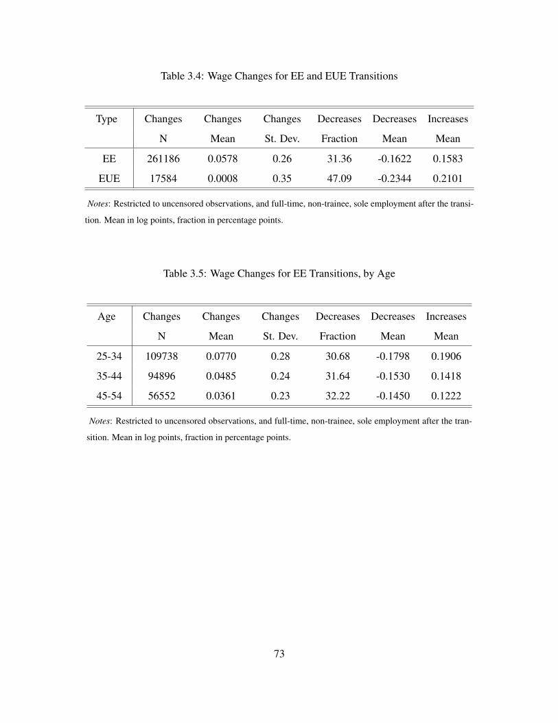
similar patterns across time and demographic groups. The fraction of wage cuts for EE transitions,

31%, is not drastically higher than for within-spell changes, 26%. In contrast, the fraction of cuts

is 47% for EUE transitions.

One group of explanations wage cuts associated with EE transitions posits that workers move

to a new job to escape a deteriorating match or to avoid an even worse situation in the future. In the

model of Moscarini (2005), continuous learning about initially unknown match quality can lead to

gradual deterioration of wages and eventual separation. In Nagypal (2005a), large shocks can lower

the value of a job, leading to an immediate separation or at least increased likelihood of a smaller

shock triggering separation. Alternatively, a reallocation shock, nicknamed ”Godfather shock,”

can force workers to choose between a random outside offer and unemployment, as in Jolivet,

Postel-Vinay and Robin (2006). Unlike a pure reallocation shock, a worsening job situation could

manifest as lowering of wages or wage growth.

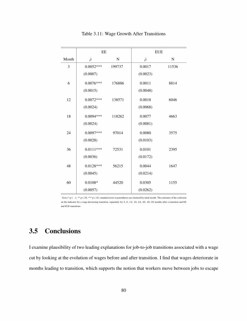
Examining the evolution of wages before separation, I find that wages deteriorate in the months

leading to separation, for all types of separations, even job-to-job transitions. The wage deteriora-

tion manifests in the year preceding transition as slower wage growth and lowering of real wages

conditioned on workers’ characteristics. Wage growth for workers who avoid separation is 3%. Be-

fore EE and EUE transitions, yearly wage growth is lower by half and two-thirds, respectively. For

other separations, wage growth is slightly negative. Real wages adjusted for workers’ characteris-

tics are lowered by 0.6% a year before separation, and lowered by 2-3% in the last pre-separation

quarter. For EE transitions, wages are lowered by 0.5% half a year before separation, and by

unemployed before or after separation and start a new job within a period of the same length are classified as makingan EUE transition.

63

around 1.5% immediately before separation. Other types of separations are preceded by more

wage deterioration. The observed wage deterioration supports the notion some of separations are

preceded by a worsening job situation, even for job-to-job transitions.

Another group of explanations proposes that workers move to a lower-paying job in the ex-

pectation of obtaining higher wages in the future. This motive arises if firms offer an increasing

wage-tenure profile, as in Coles and Burdett (2010) extension of the Burdett-Mortensen wage post-

ing model; if some firms offer attractive opportunities for accumulation of firm-specific or general

human capital; and in the Bertrand competition framework introduced in Robin and Postel-Vinay

(2002). In this framework, workers have no bargaining power, receiving take-it-or-leave-it offers

from firms. Wage growth results from the Bertrand competition in which firms engage when a

worker receives an outside offer, within the limit dictated by productivity in the current job. A

worker might make a job-to-job transition because of the option value of working for a more pro-

ductive firm with higher wage ceiling, despite the initial wage being lower.

Examining the evolution of wages after accession, I find that after EE transitions wages grow

faster for workers who accept an initial wage cut. Wage growth is negatively correlated with the

initial wage for all workers, and positively with previous wage for workers who move between

jobs. However, the finding on wage growth after EE transitions is robust to controlling for initial

and previous wages. This effect is not present for EUE transitions.

The findings of the paper suggest that both motivations for a job-to-job transition accompanied

by a wage cut are plausible. The observed wage deterioration indicates that some of separations

are preceded by a worsening job situation, even for job-to-job transitions. The positive correlation

between wage growth and the initial wage cut for job-to-job transitions suggests that at least some

of workers might accept lower initial wages in the exchange for higher future wage growth.

64

3.2 Previous Empirical Findings

Job-to-job transitions accompanied by a wage cut are a pervasive phenomenon in the labor markets.

Jolivet, Postel-Vinay and Robin (2006) use panels of worker data for 10 European countries and the

US, the European Community Household Panel and the Panel Study of Income Dynamics for the

mid-1990s. They find that the fraction of job-to-job transitions associated with a wage cut ranges

from around 18% in Portugal to 36% in Germany. The wage cuts exceed 10% for 10% to 20% of

transitions for most of the considered countries, with 29% in France, and exceed 20% for between

7% and 20% of transitions. Their explanation for these transition is the presence of reallocation

shocks, which force workers to choose between a random outside offer and unemployment.

Lopes de Melo (2007) looks at wage dynamics using the 1996 panel of the Survey of Income

Program and Participation. He finds a significant amount of wage cuts and more wage movements,

both downward and upward, in job-to-job transitions than for job stayers, with higher variance.

Wage growth is compared for workers that undertake a job-to-job transition with a wage decrease

in the first observed year and workers who keep their job initially, but experience a transition

afterwards. Wage growth is higher for the stayers in the low education group, but appears to be

lower in the high education group, supporting the notion that a wage cut might be accepted in the

expectation of higher future wages. The caveat is, however, a small sample size: the 4-year wage

growth is examined for 134 job-to-job transitions with wage cuts in the low education group and

34 in the high education group.

Tjaden and Wellschmied (2014) find that one third of job-to-job transitions are associated with

a wage cut in data from the Survey of Income and Program Participation for the 1993-1995 and

1996-1999. Additionally, workers who experience a wage cut are more likely to change jobs again.

Canon and Pavan (2014) investigate what happens to wages of workers before they make a job-

65

to-job transition. They use two measures of compensation from the National Longitudinal Survey

of Youth datasets 1979: usual wages earned and total labor earnings during the previous year.

They find evidence that wages decrease before a job-to-job transition, and argue that experiencing

a negative productivity and wage shock are more likely to change jobs. Additionally, they use the

1996 panel of the Survey of Income and Program Participation to investigate dynamics of monthly

labor income. They use dummies for future and past labor market transitions within the next 6

months and the previous 6 months. Workers who experience a transition in the recent past or the

imminent future experience a within-job wage growth 1% lower than stayers, in both cases.

Additional explanations for job-to-job transitions accompanied by wage cuts were investigated.

Workers might make a transition for non-pecuniary reasons, moving to a job that they value more

despite worse pay. Fujita (2010) finds that in the UK workers who are unsatisfied with non-

pecuniary characteristics of their job are roughly half of workers who search on the job and give job

dissatisfaction as a reason. The workers unsatisfied for non-pecuniary reasons obtain on average

lower wages conditional on moving than workers who search on the job due to low pay. Hall and

Mueller (2018) find that non-wage value of a job plays an important role for the job-acceptance

decisions of unemployed job seekers in the US. Sorkin (2018) finds evidence for movement to

lower-paying firms suggestive of compensating differentials in US administrative data. Addition-

ally, the observed wage cuts might be an artifact of measurement error, which was investigated in

Canon and Pavan (2014).

66

3.3 Data

I use German administrative microdata, the Sample of Integrated Labour Market Biographies for

1975-2010, which is 2% sample of German workers3 provided by the Research Data Centre of the

Federal Employment Agency at the Institute for Employment Research. A detailed description of

the dataset is provided in vom Berge, Koenig and Seth (2013).

For each worker, I have information on all employment spells covered by social security be-

tween 1975 and 2010: an establishment identifier, sex, education, location, working hours (full-

time or part-time), employment status (indicators for special status such as traineeship, partial

retirement and others), daily earnings, and other information. Job tenure can be precisely calcu-

lated. Every time conditions of employment change, a notification has to be submitted to the social

security system. Consequently, workers are observed at effectively daily frequency.

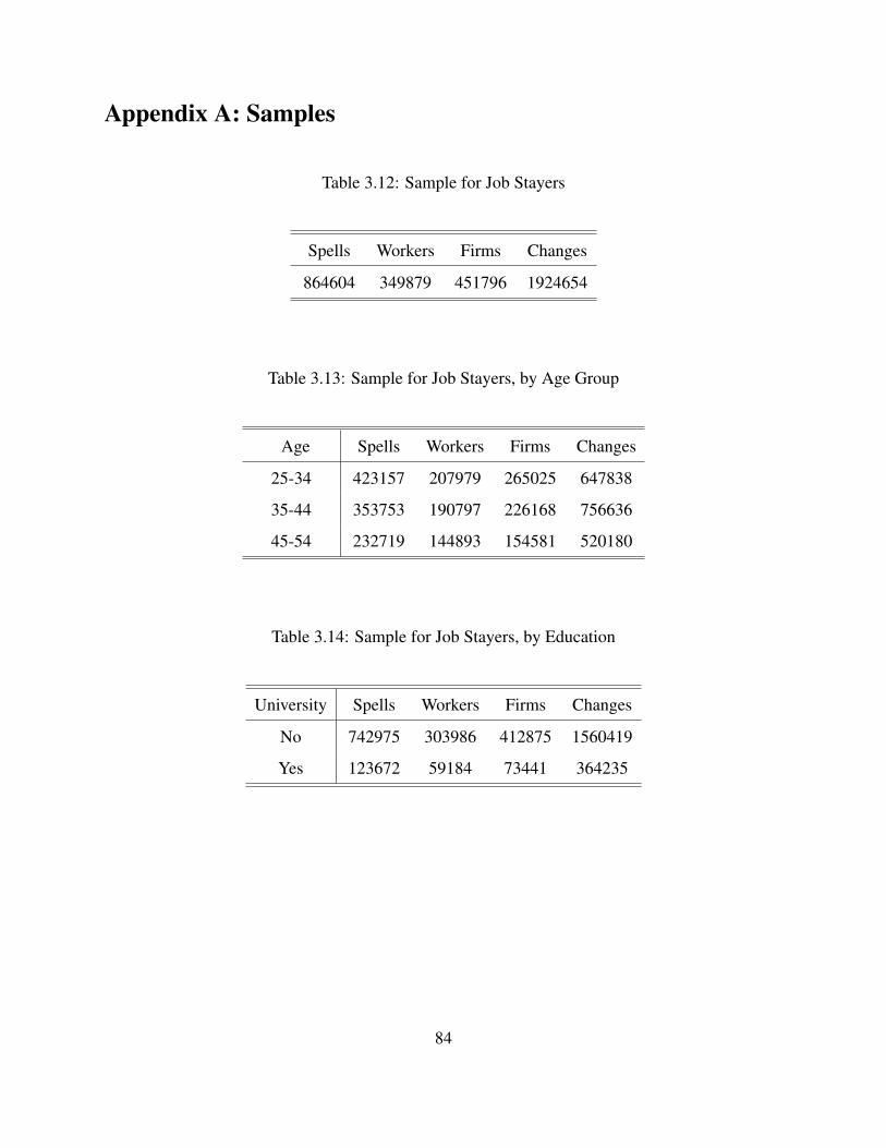
I restrict the sample to men between 25 and 54 years of age. The restriction is adopted for com-

parability with earlier studies. The lower bound of 25 years is customary, the upper bound of 54

years is lower than the usual bound of 60 years, in this case chosen to avoid issues raised by early

retirement. I further restrict the sample to employment spells in which a worker is employed con-

tinuously (with no gaps), as a full-time non-trainee, and without any parallel employment. Such

spells are more than a half of all employment spells. To calculate wage changes associated with

movement to a different job, I restrict the sample to movement to jobs in which a worker is initially

employed as a full-time non-trainee, and without any parallel employment. To investigate wage

dynamics after movement to a different job, I restrict the sample to movement from jobs in which

a worker was employed at the end of a spell as a full-time non-trainee, and without any parallel

employment. The observations with daily earnings above the legally mandated contribution as-

3Individuals appear in underlying data if at least once in the 1975-2010 period they are employees covered by thesocial security system or register as unemployed, job seekers or benefit recipients.

67

sessment ceiling (Beitragsbemessungsgrenze) are top-coded. Wages are defined as nominal daily

earnings of full-time workers. I calculate wage changes within and between employment spells

only for uncensored observations.

3.4 Empirical Results

This section starts with statistics on wage changes within employment spells, which serve as a

benchmark for wage changes associated with transitions. Then, dynamics of wages before separa-

tions and after accessions are examined.

3.4.1 Wage Changes Within Employment Spells

To provide a benchmark for wage changes experienced by workers moving between jobs, I estab-

lish the properties of wage changes within employment spells. The fraction of wage cuts is 26%

for all workers and stable across age groups, but much lower, 15%, for university-educated workers

than for the rest. Over the considered period, the fraction of wage cuts shows an upward trend. The

mean and dispersion of wage changes is higher for younger and less educated workers. Overall,

the mean wage change is 3%, with the standard deviation of 0.14. The mean wage decrease is

-8.7% and the mean wage increase is 7.1%. The results are summarized in Table 3.1.

For workers aged 25-34, 35-44, 45-54, the fraction of cuts is similar, close to 26%. Wage

changes are on average larger and more dispersed for the youngest workers. The results are sum-

marized in Table 3.2.

When workers are divided into groups with and without university education, the fraction of

cuts turns out to be much lower, 15%, in the high-education group, than in the low-education group,

28%. For the high-education group, wages changes are slightly larger with smaller dispersion. The

68

results are summarized in Table 3.3.

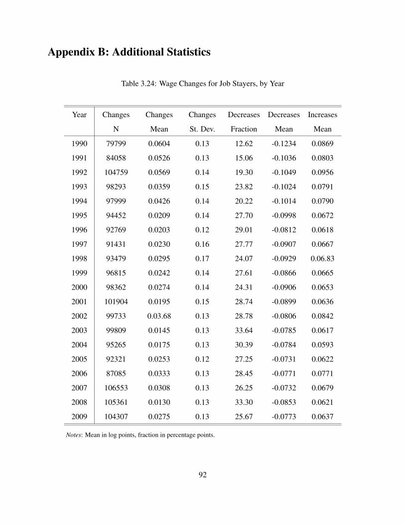
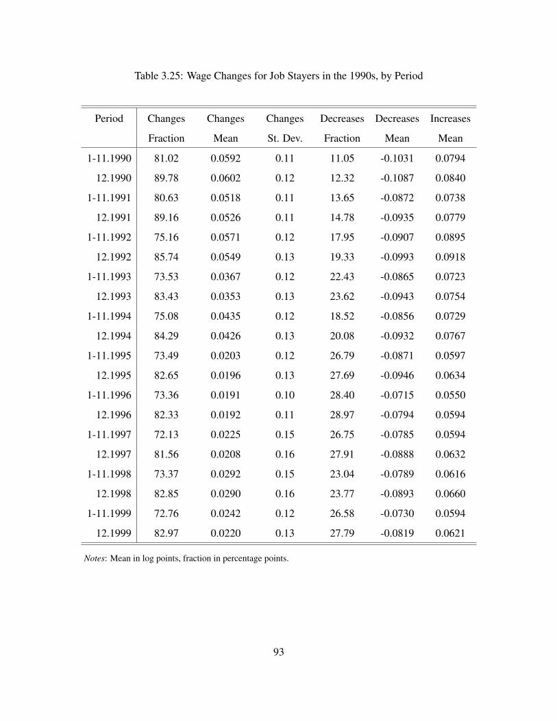
Since the sample covers 20 years, the properties of wage changes might have changed over

time. The statistics computed for each year separately turn out to be relatively stable over time,

excluding the first five years of the considered period. However, the fraction of cuts was higher in

the 2000s than the 1990s, 28% to 22%. In years 1990-1994, the fraction of cuts was noticeably

lower, 13%-24% in a year, than in 1995-2009, when it ranged from 24% to 34%. The mean and

dispersion of wage changes was slightly lower the later decade. The mean of wage changes in

1990-1994 ranged from 3.6% to 6%, in 1995-2009, from 1.3% to 3.7%. Unsurprisingly, the mean

wage change was the lowest in 2008, with the fraction of decreases close to the maximum observed

in the whole period. The results are summarized in Table 3.24.

The wage changes are not distributed uniformly over a year. More than 40% of all wage

changes observed in a year happen in December. The December wage changes have slightly higher

standard deviation and fraction of wage decreases. However, the differences are small. The results

are summarized in Table 3.25.

Table 3.1: Wage Changes for Job Stayers

Changes Changes Changes Decreases Decreases Increases

N Mean St. Dev. Fraction Mean Mean

1924654 0.0302 0.14 25.88 -0.0873 0.0713

Notes: Mean in log points, fraction in percentage points.

69

Table 3.2: Wage Changes for Job Stayers, by Age Group

Age Changes Changes Changes Decreases Decreases Increases

N Mean St. Dev. Fraction Mean Mean

25-34 647838 0.0405 0.16 25.88 -0.1001 0.0896

35-44 756636 0.0268 0.13 25.74 -0.0826 0.0647

45-54 520180 0.0224 0.12 26.08 -0.0783 0.0579

Notes: Mean in log points, fraction in percentage points.

Table 3.3: Wage Changes for Job Stayers, by Education

University Changes Changes Changes Decreases Decreases Increases

N Mean St. Dev. Fraction Mean Mean

No 11560419 0.0286 0.14 28.36 -0.0888 0.0750

Yes 364235 0.0374 0.12 15.27 -0.0750 0.0576

Notes: Mean in log points, fraction in percentage points.

3.4.2 Wage Changes for Transitions

For transitions, the fraction of wage cuts is 31% for EE transitions and 47% for EUE transitions.

The fraction of wage cuts for EE transitions is not drastically higher than 26% found for within-

spell wage changes. The mean wage change for EE transitions, 5.8%, is almost twice the mean

for within-spell changes, and dispersion is correspondingly higher. For EUE transition, the mean

wage change is 0.1% and dispersion is much higher than for EE transitions and job stayers. The

results are summarized in Table 3.4.

70

Across age and education groups, wage changes associated with EE transitions show similar

patterns to within-spell changes. The fraction of cuts is similar for workers aged 25-34, 35-44, 45-

54, but higher for low-education workers, 33%, than for high-education workers, 26%. The mean

and dispersion of changes are larger for younger workers, the mean is slightly, and dispersion

noticeably, larger for low-education than for high-education workers. The results are summarized

in Tables 3.5 and 3.6.

As for within-spell wage changes, the fraction of cuts associated with EE transitions shows an

upward trend in 1990-2009, while the mean and dispersion were relatively stable. In contrast to

within-spell changes, the fraction of cuts for EE transitions, was below the mean, 29%, in 2008,

but reached the maximum in the sample, 36.6%, in 2009, with the smallest observed mean. The

results are summarized in Table 3.26.

EE transitions are less concentrated in December than within-spell wage changes, with 26% on

average happening at the end of year. The mean and dispersion of wage changes, and the fraction

of wage cuts, are higher in the January-November period than in December An exception was

2009, when the mean change in the first 11 months was roughly equal to the mean for December,

with the fraction of cuts reaching the maximum in the sample. The results are summarized in Table

3.27.

Figures 3.1 and 3.2 show the distributions of wage changes within spells and for EE and EUE

transitions.

71

Figure 3.1: Wage Changes

Figure 3.2: Wage Changes in December

72

Table 3.4: Wage Changes for EE and EUE Transitions

Type Changes Changes Changes Decreases Decreases Increases

N Mean St. Dev. Fraction Mean Mean

EE 261186 0.0578 0.26 31.36 -0.1622 0.1583

EUE 17584 0.0008 0.35 47.09 -0.2344 0.2101

Notes: Restricted to uncensored observations, and full-time, non-trainee, sole employment after the transi-

tion. Mean in log points, fraction in percentage points.

Table 3.5: Wage Changes for EE Transitions, by Age

Age Changes Changes Changes Decreases Decreases Increases

N Mean St. Dev. Fraction Mean Mean

25-34 109738 0.0770 0.28 30.68 -0.1798 0.1906

35-44 94896 0.0485 0.24 31.64 -0.1530 0.1418

45-54 56552 0.0361 0.23 32.22 -0.1450 0.1222

Notes: Restricted to uncensored observations, and full-time, non-trainee, sole employment after the tran-

sition. Mean in log points, fraction in percentage points.

73

Table 3.6: Wage Changes for EE Transitions, by Education

University Changes Changes Changes Decreases Decreases Increases

N Mean St. Dev. Fraction Mean Mean

No 215539 0.0588 0.27 32.60 -0.1716 0.1702

Yes 45647 0.0532 0.20 25.51 -0.1057 0.1076

Notes: Restricted to uncensored observations, and full-time, non-trainee, sole employment after the transition.

Mean in log points, fraction in percentage points.

3.4.3 Pre-Separation Wage Dynamics

The evolution of wages before separation is investigated to examine whether movement between

jobs, in particular job-to-job transitions, are induced by worsening of an existing match. I find that

wages deteriorate in the months leading to separation, for all types of separations. The deterioration

is visible in lowered wage growth in the year preceding separation, and as lowered wage levels.

For EE transitions, the deterioration is weaker, but still present.

The yearly mean wage growth is 3% for workers who avoid separation, 1.8% for workers who

make an EE transition, 0.9% for workers who make an EUE transition, and -0.1 for workers who

undergo separation of different type, as shown in Table 3.7.

To check if differences in wage growth are not driven by composition of workers’ groups, I

estimate the equation

∆log wit = αEEit + αEUEit + αSit + βxit + εit (3.1)

where ∆log wit is the year-on-year difference in log wages for worker i in month t, αEEit , αEUEit ,

αSit are fixed effects for undergoing an EE transition, an EUE transition, or other separation, re-

spectively. The vector of controls, xit, contains tenure, an education-specific quadratic polynomial

74

in age, and federal state and month fixed effects. The results from the regression, shown in Table

3.8, indicate that the differences in wage growth are robust to controlling for compositional effects.

The deterioration in wages is stronger immediately before separation. To examine the evolution

of wages in the year before separation, I estimate the equation

log wit =J∑j=1

0∑k=−12

δj,kit + βyit + εit (3.2)

where wit is wage for worker i in month t, δj,kit are fixed effect for months in which worker i is k

months before separation of type j. The vector of controls, yit, contains a quadratic polynomial

in tenure, an education-specific cubic polynomial in age, and federal state and month fixed effects,

and a match fixed effect specific for a worker-firm pair. Equation 3.2 conditions wages on workers’

characteristics, average wages for a worker-firm pair and the overall wage level. Consequently, the

fixed effects for pre-separation months capture deterioration in expected real wages.

The results from the estimation of Equation 3.2 without differentiating between separations,

shown in column (1) of Table 3.9, indicate that on average wages are the lower, the closer is sepa-

ration, with deterioration by 0.6% a year before separation, and by 2-3% in the last pre-separation

quarter. The results from the estimation of Equation 3.2 with separations divided between EE

transitions, EUE transitions and other separations, shown in columns (2)-(4) of Table 3.9, indicate

that for EE transitions the deterioration starts later and is weaker than for other transitions. The

differences between EUE transitions and remaining separations are small.

Wage dynamics before job-to-job transitions with a gap of 0-9 days are markedly different than

for other separations. Additional regressions estimated, but not included, for workers undergoing

movement between jobs with and without unemployment registration with an employment gap of

10-31 and 32-93 days show that pre-separation wage dynamics for these group are similar to wage

dynamics preceding EUE with a gap of 0-9 days.

75

Table 3.7: Wage Growth Pre-Separation

Status N Mean St. Dev.

Stayers 19229442 0.0302 0.0952

EE 157582 0.0177 0.1345

EUE 9181 0.0089 0.1658

Other 145317 -0.0007 0.1992

Table 3.8: Pre-Separation Wage Growth

αEE αEUE αS

-0.0169*** -0.0196*** -0.0352***

(0.0018) (0.0022) (0.0016)

Notes:* p< .1, ** p<.05, *** p<.01; month-clustered standard errors in parentheses; 18908000 monthly

observations for 424238 worker-firm pairs, 265093 workers, 237397 firms, 149306 EE transitions, 8546 EUE

transitions and 139271 remaining separations.

76

Table 3.9: Pre-Separation Wage Dynamics

(1) (2) (3) (4)

Month All Separations EE Transitions EUE Transitions Other Separations

0 -0.0292*** -0.0155*** -0.0349*** -0.0436***

(0.0015) (0.0014) (0.0017) (0.0015)

1 -0.0253*** -0.0135*** -0.0324*** -0.0383***

(0.0012) (0.0013) (0.0015) (0.0012)

2 -0.0224*** -0.0121*** -0.0310*** -0.0343***

(0.0010) (0.0012) (0.0014) (0.0010)

3 -0.0189*** -0.0092*** -0.0280*** -0.0302***

(0.0009) (0.0010) (0.0011) (0.0009)

4 -0.0169*** -0.0080*** -0.0262*** -0.0274***

(0.0008) (0.0009) (0.0011) (0.0008)

5 -0.0152*** -0.0068*** -0.0245*** -0.0251***

(0.0007) (0.0009) (0.0010) (0.0008)

6 -0.0129*** -0.0050*** -0.0230*** -0.0223***

(0.0007) (0.0008) (0.0010) (0.0007)

7 -0.0113*** -0.0039*** -0.0213*** -0.0202***

(0.0006) (0.0007) (0.0011) (0.0007)

8 -0.0096*** -0.0026*** -0.0194*** -0.0180***

(0.0006) (0.0007) (0.0010) (0.0007)

9 -0.0075*** -0.0009 -0.0181*** -0.0154***

(0.0005) (0.0006) (0.0009) (0.0006)

10 -0.0060*** 0.0003 -0.0172*** -0.0134***

(0.0004) (0.0006) (0.0009) (0.0006)

11 -0.0052*** 0.0009 -0.0174*** -0.0121***

(0.0004) (0.0006) (0.0009) (0.0005)

12 -0.0058*** -0.0015*** -0.0166*** -0.0104***

(0.0004) (0.0005) (0.0009) (0.0004)

Notes:* p< .1, ** p<.05, *** p<.01; month-clustered standard errors in parentheses; 25891874 monthly observations for 790450 worker-firm

pairs, 341403 workers, 414361 firms, with 259029 EE transitions, 18667 EUE transitions and 512754 remaining separations. The estimates of fixed

effects for months pre-separation, from estimation for pooled separations in column (1) and for separations divided into 3 groups in columns (2)-(4).

77

3.4.4 Wage Dynamics After Transitions

The evolution of wages after movement between jobs is investigated to examine the plausibility

of the hypothesis that job-to-job transitions with wage cuts are undertaken in the expectation of

obtaining higher wages in the future. I find that for EE transitions wage growth is higher for

transitions associated with a wage cut.

Wages of workers whose wages initially decreased grow on average faster, for both EE and

EUE transitions, as summarized in Table 3.10. In general, wage growth is negatively correlated

with the initial wage, and, for workers who move between jobs, positively with previous wage.

Consequently, higher wage growth for transitions associated with a cut is expected. To check if

the relationship between wage cuts and subsequent growth is not fully driven by the initial and

preceding wages, I estimate the equation

∆klog wit = ρkit + βkzit + εkit (3.3)

where ∆klog wit is the difference of log wages of worker i in month t and month t − k, and

ρkit is a fixed effect for starting a job with lower wage than in the previous job. The vector of

controls, zit, contains tenure, an education-specific quadratic polynomial in age, and federal state

and month fixed effects, and initial and previous wages. The estimates of ρkit from estimating

Equation 3.3 separetely for workers making EE or EUE transitions and for k-month wage growth,

where k ∈ {3, 6, 12, 18, 24, 36, 48, 60}, are shown in Table 3.11.

The results for EE transitions indicate that wages of workers who accepted a wage cut grow

faster. After 3 months, the estimated difference in growth is 0.5%, with the raw difference of 1.9%

and the mean growth of 0.7% for all EE transitions; after 5 years, the difference in growth is 1.08%,

with the raw difference of 5.1% and the mean growth of 16.9%. The effect persists over time, but

becomes much smaller relative to overall wage growth. When the same equation is estimated for

78

EUE transitions, the wage cut fixed effects are not significant.

Table 3.10: Wage Growth After Transitions

Type Month 3 6 12 18 24 36 48 60

EE N 235177 206309 162227 137252 112942 83909 64595 50991

Mean 0.7 1.5 4.1 5.8 7.9 11.2 13.9 16.9

EE ↑ N 155999 139790 111813 95531 78938 59133 46028 36419

Mean 0.1 0.5 2.7 4.3 6.4 9.5 12.3 15.2

EE ↓ N 64677 54137 41130 34031 28052 20501 15600 12238

Mean 2.0 3.7 6.6 8.6 10.7 14.1 17.0 20.1

EUE N 13509 10225 7049 5410 4188 2795 1917 1356

Mean 1.2 2.6 5.2 7.3 9.4 13.1 16.5 19.0

EUE ↑ N 6685 5229 3746 2903 2242 1490 1018 729

Mean 0.7 1.7 3.8 5.6 7.7 10.7 14.1 15.7

EUE ↓ N 5709 4129 2698 2055 1589 1070 748 521

Mean 1.8 3.8 6.7 9.2 11.0 15.0 18.3 22.1

Notes: Restricted to uncensored observations, and full-time, non-trainee, sole employment after the transition.

Mean in log points. The signs ↑ and ↓ indicate transitions associated with wage increases and decreases.

79

Table 3.11: Wage Growth After Transitions

EE EUE

Month ρ N ρ N

3 0.0052*** 199737 0.0017 11536

(0.0007) (0.0023)

6 0.0076*** 176886 0.0011 8814

(0.0015) (0.0048)

12 0.0072*** 138571 0.0018 6046

(0.0024) (0.0068)

18 0.0094*** 118262 0.0077 4663

(0.0024) (0.0081)

24 0.0097*** 97014 0.0080 3575

(0.0028) (0.0103)

36 0.0111*** 72531 0.0101 2395

(0.0036) (0.0172)

48 0.0128*** 56215 0.0044 1647

(0.0045) (0.0214)

60 0.0108* 44520 0.0305 1155

(0.0057) (0.0262)

Notes:* p< .1, ** p<.05, *** p<.01; standard errors in parentheses are clustered by intial month. The estimates of the coeficient

on the indicator for a wage-decreasing transition, separately for 3, 6, 12, 18, 24, 36, 48, 60 months after a transition and EE

and EUE transitions.

3.5 Conclusions

I examine plausibility of two leading explanations for job-to-job transitions associated with a wage

cut by looking at the evolution of wages before and after transition. I find that wages deteriorate in

months leading to transition, which supports the notion that workers move between jobs to escape

80

a deteriorating match. However, wages grow faster for workers who accepted wage cuts, at least

after job-to-job transitions. Wage growth after movement between jobs associated with even short

unemployment is not positively associated with a wage cut.

Taken together, the findings suggest that both transitions induced by worsening of an existing

match, and acceptance of lower initial wage in the exchange for higher future wage growth are

present in the labor market.

81

Bibliography

[1] Canon, Maria, and Ronni Pavan. 2014. ”Wage dynamics and labor market transitions: a

reassessment through total income and “usual” wages.” Federal Reserve Bank of St. Louis

Working Paper Series.

[2] Burdett, Ken, and Melvyn Coles. 2010. ”Wage/tenure contracts with heterogeneous firms.”

Journal of Economic Theory 145(4): 1408-1435.

[3] Connolly, Helen, and Peter Gottschalk. 2008. ”Wage Cuts as Investment in Future Wage

Growth.” Labour 22(1): 1-22.

[4] Fujita, Shigeru. 2010. ”An empirical analysis of on-the-job search and job-to-job transitions.”

Working Papers 10-34, Federal Reserve Bank of Philadelphia, revised 01 Aug 2012.

[5] Jolivet, Gregory, Fabien Postel-Vinay, and Jean-Marc Robin. 2006. ”The empirical content

of the job search model: Labor mobility and wage distributions in Europe and the US.”

European Economic Review 50(4): 877-907.

[6] Hall, Robert and Andreas Mueller. 2018. ”Wage Dispersion and Search Behavior: The

Importance of Nonwage Job Values.” Journal of Political Economy 126(4): 1594-1637.

[7] Lopes de Melo, Rafael. 2007. ”Theories of Wage Determination and Wage Dynamics: An

Empirical Assessment.” mimeo.

82

[8] Moscarini, Giuseppe. 2005. ”Job Matching and the Wage Distribution.” Econometrica 73(2):

481-516.

[9] Nagypal, Eva. 2005a. ”On the extent of job-to-job transitions.” Manuscript, Northwestern

University.

[10] Nagypal, Eva. 2005a. ”Worker reallocation over the business cycle: The importance of

job-to-job transitions.” Manuscript, Northwestern University.

[11] Postel-Vinay, Fabien, and Jean-Marc Robin. 2002. ”Equilibrium Wage Dispersion with

Worker and Employer Heterogeneity.” Econometrica 70(6): 2295-2350.

[12] Sorkin, Isaac. 2018. ”Ranking Firms Using Revealed Preference.” Quarterly Journal of

Economics 133(3): 1331–1393.

[13] Tjaden, Volker, and Felix Wellschmied. 2014. ”Quantifying the Contribution of Search to

Wage Inequality.” American Economic Journal: Macroeconomics 6(1): 134-161.

[14] vom Berge, Philipp, Marion Koenig, and Stefan Seth. 2013. ”Sample of Integrated Labour

Market Biographies (SIAB) 1975-2010.” FDZ Datenreport. Documentation on Labour Mar-

ket Data from Institut fur Arbeitsmarkt- und Berufsforschung (IAB), Nuernberg.

83

Appendix A: Samples

Table 3.12: Sample for Job Stayers

Spells Workers Firms Changes

864604 349879 451796 1924654

Table 3.13: Sample for Job Stayers, by Age Group

Age Spells Workers Firms Changes

25-34 423157 207979 265025 647838

35-44 353753 190797 226168 756636

45-54 232719 144893 154581 520180

Table 3.14: Sample for Job Stayers, by Education

University Spells Workers Firms Changes

No 742975 303986 412875 1560419

Yes 123672 59184 73441 364235

84

Table 3.15: Sample for Job Stayers, by Year

Year Spells Workers Firms Changes

1990 109557 97969 66640 79799

1991 116279 104876 71270 84058

1992 154365 137149 94444 104759

1993 148404 133155 94775 98293

1994 145565 130626 95200 97999

1995 142544 128148 94250 94452

1996 140443 126828 93163 92769

1997 138613 125221 92749 91431

1998 138359 124929 92299 93479

1999 141756 126688 94391 96815

2000 145365 128756 95755 98362

2001 144415 129120 94594 101904

2002 138223 125810 90384 99733

2003 l32571 122165 86440 99809

2004 129430 119752 83794 95265

2005 126958 117607 81802 92321

2006 130948 120106 83236 87085

2007 137451 124400 86697 106653

2008 140696 127759 88312 105361

2009 139163 127665 68064 104307

85

Table 3.16: Sample for Job Stayers in the 1990s, by Period

Period Spells Workers Firms Changes

1-11.1990 108392 97332 65961 754773

12.1990 86297 86249 51582 77595

1-11.1991 115257 104322 70621 809611

12.1991 92093 92053 55531 82212

1-11.1992 152955 136526 93534 995873

12.1992 118114 118036 72544 101488

1-11.1993 147022 132537 93867 942189

12.1993 113984 113903 72635 95288

1-11.1994 144013 129907 94168 942265

12.1994 113408 113291 73960 95732

1-11.1995 141071 127422 93341 902713

12.1995 110858 110771 72923 91804

1-11.1996 139125 126175 92918 893365

12.1996 108968 108898 72441 90628

1-11.1997 137106 124500 91853 867614

12.1997 107432 107364 71793 88738

1-11.1998 136796 124127 91343 879824

12.1998 108278 108192 72217 90880

1-11.1999 140160 125922 93398 886092

12.1999 109925 109827 73530 92232

86

Table 3.17: Sample for Job Stayers in the 2000s, by Period

Period Spells Workers Firms Changes

1-11.2000 143575 127964 94714 909889

12.2000 111731 111627 73874 94829

1-11.2001 142996 128496 93736 918378

12.2001 111326 111244 72972 94010

1-11.2002 136965 125240 89592 908601

12.2002 108538 108468 70659 91622

1-11.2003 131365 121569 85713 888462

12.2003 106666 106603 69203 89448

1-11.2004 128240 119156 83048 874607

12.2004 105020 104969 67821 88326

1-11.2005 125682 116978 81032 850271

12.2005 105051 104985 67476 86984

1-11.2006 129561 119368 82432 776849

12.2006 108380 108298 69380 81453

1-11.2007 136032 123723 85892 936401

12.2007 112095 112017 71422 97138

1-11.2008 139421 127144 87539 968412

12.2008 115300 115239 73004 100112

1-11.2009 137857 127016 87283 953449

12.2009 115046 114969 73289 98094

87

Table 3.18: Sample for Separations

Spells Workers Firms EE EUE Other

757159 320122 412558 271548 19318 466293

Table 3.19: Sample for Separations, by Age

Age Spells Workers Firms EE

25-34 318634 156033 217089 113941

35-44 246446 128996 176252 97579

45-54 148994 86425 111079 58043

Table 3.20: Sample for Separations, by Education

University Spells Workers Firms EE

No 659341 279922 377604 224103

Yes 97818 49823 62090 47445

88

Table 3.21: Sample for Separations, by Year

Year Spells Workers Firms EE

1990 30378 25710 25269 11876

1991 31924 27609 26616 11973

1992 47956 41950 37092 19109

1993 47038 41432 36944 17067

1994 45284 39690 36316 16259

1995 45224 39803 35755 17203

1996 43079 37878 34901 14486

1997 42098 37061 34369 13657

1998 40661 36141 33352 14440

1999 41438 36406 34046 15501

2000 43417 37938 35434 17561

2001 42637 37416 34991 16096

2002 38567 34203 31577 13277

2003 33602 30141 27671 10501

2004 31617 28538 25984 9667

2005 28573 25689 23552 8846

2006 28954 25858 23319 10412

2007 31322 27720 25160 12402

2008 31899 28005 25730 11764

2009 31491 27919 25359 9451

89

Table 3.22: Sample for Separations in the 1990s, by Period

Period Spells Workers Firms EE

1-11.1990 24985 21135 21399 9279

12.1990 5393 5386 4670 2597

1-11.1991 26177 22650 22547 9231

12.1991 5747 5744 4952 2742

1-11.1992 38279 33551 31067 14230

12.1992 9677 9667 7489 4879

1-11.1993 37001 32644 30538 12222

12.1993 10037 10031 7732 4845

1-11.1994 34921 30677 29404 11690

12.1994 10363 10341 8252 4569

1-11.1995 33784 29622 28857 11512

12.1995 11440 11431 8164 5691

1-11.1996 33842 29860 28853 10164

12.1996 9237 9231 7149 4322

1-11.1997 33079 29211 28130 9731

12.1997 9019 9011 7293 3926

1-11.1998 31765 28355 27126 10363

12.1998 8896 8888 7257 4077

1-11.1999 33461 29621 28229 11723

12.1999 7977 7967 6894 3778

90

Table 3.23: Sample for Separations in the 2000s, by Period

Period Spells Workers Firms EE

1-11.2000 35076 30916 29552 13245

12.2000 8341 8332 6979 4316

1-11.2001 34358 30343 29121 12031

12.2001 8279 8269 6909 4065

1-11.2002 30958 27641 26238 9568

12.2002 7609 7600 6188 3709

1-11.2003 26993 24341 23006 7561

12.2003 6609 6606 5467 2940

1-11.2004 25234 22888 21276 6948

12.2004 6383 6376 5448 2719

1-11.2005 22884 20682 19339 6512

12.2005 5689 5678 4906 2334

1-11.2006 23381 21048 19265 7783

12.2006 5573 5569 4793 2629

1-11.2007 26040 23284 21269 9810

12.2007 5282 5274 4669 2592

1-11.2008 26157 23175 21653 9342

12.2008 5742 5733 4967 2422

1-11.2009 25117 22419 20577 7300

12.2009 6374 6368 5526 2151

91

Appendix B: Additional Statistics

Table 3.24: Wage Changes for Job Stayers, by Year

Year Changes Changes Changes Decreases Decreases Increases

N Mean St. Dev. Fraction Mean Mean

1990 79799 0.0604 0.13 12.62 -0.1234 0.0869

1991 84058 0.0526 0.13 15.06 -0.1036 0.0803

1992 104759 0.0569 0.14 19.30 -0.1049 0.0956

1993 98293 0.0359 0.15 23.82 -0.1024 0.0791

1994 97999 0.0426 0.14 20.22 -0.1014 0.0790

1995 94452 0.0209 0.14 27.70 -0.0998 0.0672

1996 92769 0.0203 0.12 29.01 -0.0812 0.0618

1997 91431 0.0230 0.16 27.77 -0.0907 0.0667

1998 93479 0.0295 0.17 24.07 -0.0929 0.06.83

1999 96815 0.0242 0.14 27.61 -0.0866 0.0665

2000 98362 0.0274 0.14 24.31 -0.0906 0.0653

2001 101904 0.0195 0.15 28.74 -0.0899 0.0636

2002 99733 0.03.68 0.13 28.78 -0.0806 0.0842

2003 99809 0.0145 0.13 33.64 -0.0785 0.0617

2004 95265 0.0175 0.13 30.39 -0.0784 0.0593

2005 92321 0.0253 0.12 27.25 -0.0731 0.0622

2006 87085 0.0333 0.13 28.45 -0.0771 0.0771

2007 106553 0.0308 0.13 26.25 -0.0732 0.0679

2008 105361 0.0130 0.13 33.30 -0.0853 0.0621

2009 104307 0.0275 0.13 25.67 -0.0773 0.0637

Notes: Mean in log points, fraction in percentage points.

92

Table 3.25: Wage Changes for Job Stayers in the 1990s, by Period

Period Changes Changes Changes Decreases Decreases Increases

Fraction Mean St. Dev. Fraction Mean Mean

1-11.1990 81.02 0.0592 0.11 11.05 -0.1031 0.0794

12.1990 89.78 0.0602 0.12 12.32 -0.1087 0.0840

1-11.1991 80.63 0.0518 0.11 13.65 -0.0872 0.0738

12.1991 89.16 0.0526 0.11 14.78 -0.0935 0.0779

1-11.1992 75.16 0.0571 0.12 17.95 -0.0907 0.0895

12.1992 85.74 0.0549 0.13 19.33 -0.0993 0.0918

1-11.1993 73.53 0.0367 0.12 22.43 -0.0865 0.0723

12.1993 83.43 0.0353 0.13 23.62 -0.0943 0.0754

1-11.1994 75.08 0.0435 0.12 18.52 -0.0856 0.0729

12.1994 84.29 0.0426 0.13 20.08 -0.0932 0.0767

1-11.1995 73.49 0.0203 0.12 26.79 -0.0871 0.0597

12.1995 82.65 0.0196 0.13 27.69 -0.0946 0.0634

1-11.1996 73.36 0.0191 0.10 28.40 -0.0715 0.0550

12.1996 82.33 0.0192 0.11 28.97 -0.0794 0.0594

1-11.1997 72.13 0.0225 0.15 26.75 -0.0785 0.0594

12.1997 81.56 0.0208 0.16 27.91 -0.0888 0.0632

1-11.1998 73.37 0.0292 0.15 23.04 -0.0789 0.0616

12.1998 82.85 0.0290 0.16 23.77 -0.0893 0.0660

1-11.1999 72.76 0.0242 0.12 26.58 -0.0730 0.0594

12.1999 82.97 0.0220 0.13 27.79 -0.0819 0.0621

Notes: Mean in log points, fraction in percentage points.

93

Table 3.26: Wage Changes for Job Stayers in the 2000s, by Period

Period Changes Changes Changes Decreases Decreases Increases

Fraction Mean St. Dev. Fraction Mean Mean

1-11.2000 73.36 0.0263 0.12 23.35 -0.0764 0.0576

12.2000 83.94 0.0258 0.13 24.22 -0.0875 0.0620

1-11.2001 73.31 0.0190 0.13 27.58 -0.0767 0.0554

12.2001 83.47 0.0157 0.14 28.54 -0.0863 0.0564

1-11.2002 73.98 0.0363 0.11 28.12 -0.0703 0.0780

12.2002 83.28 0.0337 0.12 28.96 -0.0777 0.0792

1-11.2003 74.00 0.0135 0.11 32.64 -0.0666 0.0524

12.2003 82.54 0.0079 0.12 34.43 -0.0762 0.0520

1-11.2004 73.96 0.0162 0.11 29.48 -0.0670 0.0511

12.2004 82.88 0.0126 0.12 30.88 -0.0756 0.0520

1-11.2005 72.78 0.0235 0.10 26.35 -0.0612 0.0538

12.2005 81.31 0.0224 0.12 27.30 -0.0707 0.0574

1-11.2006 65.22 0.0310 0.11 28.01 -0.0646 0.0682

12.2006 74.18 0.0298 0.12 28.56 -0.0748 0.0716

1-11.2007 75.89 0.0279 0.11 25.08 -0.0616 0.0579

12.2007 85.58 0.0260 0.12 26.14 -0.0718 0.0606

1-11.2008 75.83 0.0116 0.11 32.85 -0.0759 0.0545

12.2008 85.48 0.0097 0.12 33.79 -0.0833 0.0571

1-11.2009 74.38 0.0276 0.10 24.11 -0.0653 0.0571

12.2009 83.97 0.0255 0.11 25.16 -0.0747 0.0592

Notes: Mean in log points, fraction in percentage points.

94

Table 3.27: Wage Changes for EE Transitions, by Year

Year Changes Changes Changes Decreases Decreases Increases

N Mean St. Dev. Fraction Mean Mean

1990 11133 0.0715 0.27 27.04 -0.1949 0.1702

1991 11353 0.0741 0.26 29.50 -0.1741 0.1779

1992 18463 0.1011 0.26 24.41 -0.1770 0.1910

1993 16124 0.0554 0.26 32.37 -0.1723 0.1644

1994 15596 0.0608 0.25 28.76 -0.1816 0.1587

1995 16405 0.0518 0.25 31.52 -0.1599 0.1492

1996 14178 0.0449 0.23 33.47 -0.1468 0.1413

1997 13300 0.0442 0.25 33.27 -0.1597 0.1459

1998 13948 0.0621 0.27 31.99 -0.1522 0.1629

1999 15005 0.0569 0.26 30.40 -0.1703 0.1561

2000 16983 0.0649 0.26 31.08 -0.1536 0.1634

2001 15534 0.0470 0.27 34.15 -0.1566 0.1526

2002 12868 0.0453 0.27 31.61 -0.1638 0.1419

2003 10139 0.0367 0.25 36.28 -0.1505 0.1433

2004 9340 0.0448 0.24 31.35 -0.1565 0.1367

2005 8520 0.0435 0.26 33.43 -0.1560 0.1436

2006 10007 0.0562 0.27 33.76 -0.1526 0.1626

2007 11946 0.0619 0.26 32.72 -0.1554 0.1676

2008 11322 0.0667 0.26 29.04 -0.1628 0.1606

2009 9022 0.0356 0.25 36.57 -0.1522 0.1438

Notes: Restricted to uncensored observations, and full-time, non-trainee, sole employment after the tran-

sition. Mean in log points, fraction in percentage points.

95

Table 3.28: Wage Changes for EE Transitions in the 1990s, by Period

Period Changes Changes Changes Decreases Decreases Increases

N Mean St. Dev. Fraction Mean Mean

1-11.1990 792.82 0.0726 0.29 31.05 -0.2024 0.1967

12.1990 2412 0.0690 0.19 16.38 -0.1679 0.1154

1-11.1991 787.64 0.0746 0.29 33.17 -0.1980 0.2037

12.1991 2689 0.0647 0.19 19.23 -0.1562 0.1173

1-11.l992 1255.45 0.1035 0.29 28.69 -0.1967 0.2192

12.1992 4653 0.0866 0.18 16.33 -0.1404 0.1309

1-11.l993 1045.27 0.0610 0.29 36.41 -0.1991 0.2035

12.1993 4626 0.0417 0.16 23.19 -0.1262 0.0924

1-11.l994 100.1936 0.0637 0.28 32.61 -0.1997 0.1914

12.1994 4394 0.0510 0.16 20.87 -0.1229 0.0968

1-11.1995 989.18 0.0617 0.29 37.08 -0.1785 0.2030

12.1995 5524 0.0285 0.15 22.18 -0.1107 0.0681

1-11.1996 899.09 0.0511 0.26 37.60 -0.1651 0.1930

12.1996 4288 0.0272 0.14 25.77 -0.1013 0.0718

1-11.1997 859 0.0493 0.28 36.62 -0.1776 0.1915

12.1997 3851 0.0280 0.17 27.16 -0.1086 0.0789

1-11.1998 907.73 0.0661 0.30 36.55 -0.1678 0.1997

12.1998 3963 0.0502 0.20 21.55 -0.1171 0.0962

1-11.l999 1026.27 0.0648 0.29 32.46 -0.1964 0.1953

12.1999 3716 0.0374 0.20 26.10 -0.1178 0.0923

Notes: Restricted to uncensored observations, and full-time, non-trainee, sole employment after the transi-

tion. Mean in log points, fraction in percentage points.

96

Table 3.29: Wage Changes for EE Transitions in the 2000s, by Period

Period Changes Changes Changes Decreases Decreases Increases

N Mean St. Dev. Fraction Mean Mean

1-11.2000 1160.27 0.0732 0.28 32.76 -0.1737 0.1915

12.2000 4220 0.0413 0.19 25.69 -0.1200 0.0970

1-11.2001 1049.45 0.0525 0.29 37.53 -0.1722 0.1975

12.2001 3990 0.0260 0.17 25.84 -0.1176 0.0760

1-11.2002 837 0.0433 0.30 34.97 -0.1970 0.1670

12.2002 3661 0.0480 0.16 25.92 -0.0954 0.0982

1-11.2003 658.73 0.0456 0.28 37.85 -0.1757 0.1905

12.2003 2893 0.090 0.14 33.74 -0.0981 0.0636

1-11.2004 606.73 0.0513 0.27 34.03 -0.1772 0.1686

12.2004 2666 0.0205 0.15 27.76 -0.1049 0.0688

1-11.2005 566.64 0.0470 0.28 36.10 -0.1757 0.1739

12.2005 2287 0.0338 0.19 28.60 -0.1002 0.0875

1-11.2006 675 0.0617 0.30 36.69 -0.1739 0.1974

12.2006 2582 0.0389 0.18 25.56 -0.1163 0.0922

1-11.2007 855.91 0.0655 0.28 35.05 -0.1719 0.1934

12.2007 2531 0.0482 0.19 23.94 -0.1191 0.1009

1-11.2008 813 0.0715 0.27 31.25 -0.1752 0.1930

12.2008 2379 0.0411 0.17 25.18 -0.1134 0.0930

1-11.2009 629.55 0.0354 0.27 40.43 -0.1667 0.1679

12.2009 2097 0.0352 0.18 25.04 -0.1115 0.0842

Notes: Restricted to uncensored observations, and full-time, non-trainee, sole employment after the transi-

tion. Mean in log points, fraction in percentage points.

97


Recommended