133


Essays in Real Estate Research Band 9
Edited By N. B. Rottke , Eschborn , Germany J. Mutl , Wiesbaden , Germany

Die Reihe „Essays in Real Estate Research”, herausgegeben von Professor Dr. Nico B. Rottke FRICS und Professor Jan Mutl, Ph.D. umfasst aktuelle Forschungsarbe-iten der Promovenden der Lehrstühle und Professuren des Real Estate Manage-ment Institutes der EBS Business School. Forschungs- und Lehrschwerpunkte des Institutes bilden die interdisziplinären Aspekte der Immobilientransaktion sowie die nachhaltige Wertschöpfungskette im Immobilienlebenszyklus. Die Kapital-märkte werden als essenzieller Bestandteil der Entwicklung der Immobilienmärkte aufgefasst.
Die in der Regel empirischen Studien betrachten transaktions- und kapitalmark-tnahe Th emenbereiche aus dem Blickwinkel der institutionellen Immobiliengew-erbe- und -wohnungswirtschaft , wie bspw. Finanzierung, Kapitalmarktstruktur, Investition, Risikomanagement, Bewertung, Ökonomie oder Portfoliomanage-ment, aber auch angewandte Th emen wie Corporate Real Estate Management, Projektentwicklung oder Unternehmensführung. Die ersten 11 Bände der Reihe erschienen bis 2014 auch im Immobilien Manager Verlag, Köln.
Th e series “Essays in Real Estate Research”, published by Professor Dr. Nico B. Rottke FRICS and Professor Jan Mutl, Ph.D., includes current research work of doctoral students at the chairs and professorships of the Real Estate Management Institute of EBS Business School. Th e research and teaching focus of the Institute constitutes the interdisciplinary aspects of real estate transactions as well as the sustainable value creation chain within the real estate life cycle. Th e capital markets are regarded as essential components of the development of the real estate markets.
Th e mostly empirical studies consider transactional as well as capital market top-icsfrom the point of view of the institutional commercial and residential real estate industry, such as fi nance, capital market structure, investment, risk management, valuation, economics or portfolio management, but also applied topics such as
Edited By Nico B. Rottke Ernst & Young Real Estate GmbH Eschborn , Germany
Jan Mutl EBS Business School Wiesbaden , Germany

Anna Mathieu
Essays on the Impactof Sentiment on RealEstate Investments
With a Preface of the Editors byProf. Dr. Nico B. Rottke and Prof. Dr. Matthias Thomas
Essays in Real Estate Research ISBN 978-3-658-11636-1 ISBN 978-3-658-11637-8 (eBook) DOI 10.1007/978-3-658-11637-8 Library of Congress Control Number: 2015953452 Springer Gabler Previously published by Immobilien Manager Verlag, Cologne, 2013 © Springer Fachmedien Wiesbaden 2016 This work is subject to copyright. All rights are reserved by the Publisher, whether the whole or part of the material is concerned, specifi cally the rights of translation, reprinting, reuse of illus-trations, recitation, broadcasting, reproduction on microfi lms or in any other physical way, and transmission or information storage and retrieval, electronic adaptation, computer software, or by similar or dissimilar methodology now known or hereafter developed. The use of general descriptive names, registered names, trademarks, service marks, etc. in this publication does not imply, even in the absence of a specifi c statement, that such names are exempt from the relevant protective laws and regulations and therefore free for general use. The publisher, the authors and the editors are safe to assume that the advice and information in this book are believed to be true and accurate at the date of publication. Neither the publisher nor the authors or the editors give a warranty, express or implied, with respect to the material contained herein or for any errors or omissions that may have been made. Printed on acid-free paper Springer Gabler is a brand of Springer Fachmedien Wiesbaden Springer Fachmedien Wiesbaden is part of Springer Science+Business Media (www.springer.com)
Dr. Anna Mathieu EBS Business School Wiesbaden , Germany
Unchanged Reprint 2015 Up to 2014 the title was published in Immobilien Manager Verlag, Cologne, in the series „Schriftenreihe zur immobilienwirtschaftlichen Forschung“.

Preface of the Editor V
Preface of the Editor
The tremendous downturn of the U.S. housing market was one of the
drivers for the current global financial crisis, which had originated in
the U.S. market for mortgage backed securities in 2007. Until April
2009, the crash of the U.S. banking and its related shadow banking
system, in conjunction with the confidence crisis, has caused a direct
loss of nearly 3 Trillion dollars. Once more, the asset class “real
estate” had demonstrated its crucial role in global economics.
Against this background, the current crisis of the European Monetary
Union has illustrated very well which large impact sentiment has for
stock markets as well as for physical markets: reactions of market
participants can hardly be explained with underlying fundamentals
and efficient market theory.
Thus, the author of this Ph.D.-thesis, Ms. Dipl.-Kffr. Anna Mathieu,
has chosen a very current topic which she applies in the context of
real estate, more specifically, US Real Estate Investment Trusts and
direct residential real estate in the U.S. and investigates the
sentiment of various market participants. Therefore, the main part of
her dissertation is composed of three essays investigating the impact
of sentiment on real estate investments as follows:
• Impact of Investor Sentiment on U.S. REIT returns
• Investor Sentiment and the Return and Volatility of U.S.
REITs and Non-REITs during the Financial Crisis
• Impact of Consumer Sentiment on the Number of New Home
Sales in the U.S.

VI Preface of the Editor
The first stand-alone study (chapter 2) deals with the impact of
investor sentiment on REIT returns: after an introduction which tries
to motivate the study and the topic, defined as REITS being a special
investment class, the author conducts a literature review and
summarizes the existing results of sentiment research.
In this part of the thesis, the aim of the study is characterized as an
extension of the literature on REIT returns and volatility by
considering the impact of investor sentiment on REIT returns and
volatility. The author then describes her data set and her
methodology using US Equity REIT total returns and employing
several GARCH-models with and without sentiment. The author
concludes that REIT returns and return volatility are influenced by
investor sentiment being itself asymmetric: bearish sentiment having
a stronger impact on the volatility of REITs.
The second study, chapter 3, deals with investor sentiment and the
return and volatility of REITs and Non-REITs during the financial
crisis and the hypothesis is postulated that more sales happen when
consumer sentiment is high and less sales in unstable market
environments.
In this part as well, the aim of the study is to extend the literature on
sentiment by considering the impact of institutional investor
sentiment on returns and conditional volatility of different asset
classes in an unstable market environment using U.S. Equity REIT
returns, S&P 500 returns, and NASDAQ returns. The theoretical
background of the paper is described explaining four different effects
(the “holdmore- effect”, the “price pressure effect”, the “create space
effect” as well as the “Friedman effect”) which are then empirically
tested using the aforementioned data in connection with a GARCH-
M model. The hypothesis is stated that market sentiment has a higher
impact in extreme market environments such as the 2008-financial
crisis. The hypothesis is then tested and confirmed (with the
Preface of the Editor IIV
exception of NASDAQ-returns) using the aforementioned effects as
explanations.
The third study of this thesis, the fourth chapter of the disseration,
analyzes the impact of consumer sentiment on the number of new
home sales. At this point, the object of study changes from indirect
real estate – REITs – to direct real estate though.
The aim of the study is described with the investigation if consumer
sentiment has an impact on the decision of a household to buy a new
home. After a brief literature review, the author uses a data set from
1978 to 2010 is used with a total of 385 monthly observations from
the Federal Reserve Bank of St. Louis. Methodologically,
unobserved component models (instead of OLS regressions) are used
to utilize their advantage to identify coefficients of some observable
determinants of the dependent variable even if some independent
variables are omitted. Results show that consumer (here instead of
investor) sentiment has a significantly positive impact on the number
of new one-family home sales in the U.S.
Next to consumer sentiment, the mortgage rate is identified as
critical variable with a strong and significant impact.
The analysis thereby illustrates that 2008-financial crisis cannot be
predicted by the data.
The dissertation at hand has been accepted at EBS Business School
in autumn 2011 and graded with distinction. It provides practical
results for investigating the sentiment of two different market
participants (investors and consumers) in the U.S. residential market
and shows up room for further research to be conducted against this
background.

IIIV Preface of the Editor
Therewith, we sincerely do hope that this research project will be
well appreciated by both, real estate researchers and practitioners,
alike.
Wiesbaden, November 21st, 2012
Prof. Dr. Nico Rottke FRICS CRE Prof. Dr. Matthias Thomas MRICS
Aareal Endowed Chair Endowed Chair Real Estate Investment & Finance Real Estate Management Real Estate Management Institute EBS Business School EBS Universität für Wirtschaft und Recht

Preface of the Author IX
Preface of the Author
The dissertation at hand was created in the years 2008 to 2011
during the time as internal doctorate candidate at the Endowed Chair
of Real Estate Investment and Finance of Prof. Dr. Nico B. Rottke at
Real Estate Management Institue at the former European Business
School – now EBS Business School -
Many people supported me during the time of my dissertation and I
like to to express my greatest gratitude to them.
However, the greatest gratitude is dedicated to my family, first and
foremest my father and my mother who always believed in me and
who made this education possible at all. Both experienced all up and
downs in the creation of this doctoral thesis and supported me with
motivation and energy. Also, I’d like to thank my husband Matthias,
who moved close to my parents during my disseration and
pregnancy with our first daughther Charlotte as a favor for me. In
return, he did not only accept additional traveling but also supported
me with spiritual succor to finsish this work successfully. Finally, I
like to express my gratitude to my siblings Ulf and Elise for their
motivation and the recessary provision of diversion in desperate
times.

X Preface of the Author
In particular I have to thank my doctoral advisor and academic
teacher Mr. Prof. Dr. Nico B. Rottke as well as my second referee
Mr. Prof. Dr. Joachim Zietz for their acadamic supervision of my
work.
Both supervisors were always available to me and did actively
support me at anytime. Professor Rottke gave me the required
academic liberty in the creation process and supported my progress
with valuable discussions. Despite the huge spatial distance to
Professor Zietz in the United States of Amercia and the given time
lag he was a great constant I could count on at anytime though.
I received great support from my doctoral fellows at the Endowed
Chair of Real Estate Investment and Finance: I was able to discuss
the content of my thesis in several doctoral seminars and
conversations and got very useful hints and advice.
Dr. Anna Mathieu

Content Overview IX
Table of Contents
Preface of the Editor...........................................................................V
Preface of the Author ........................................................................IX
Table of Contents ............................................................................. XI
List of Abbreviations....................................................................... XV
List of Figures .............................................................................. XVII
List of Tables .................................................................................. XIX
1 Introduction ..................................................................................... 1
2 The Impact of Investor Sentiment on REIT Returns ...................... 9
2.1 Introduction ................................................................ 9
2.2 Literature Review ..................................................... 12
2.3 Data and Methodology ............................................. 17
2.3.1 Data ............................................................................ 17
2.3.2 The GARCH Model without Sentiment ..................... 18
2.3.3 The Sentiment Threshold GARCH Model ................. 19
2.4 Empirical Results...................................................... 20
2.4.1 Augmented Dickey-Fuller Test and KPSS Test......... 21
2.4.2 Summary Statistics ..................................................... 21
2.4.3 The GARCH Model without Sentiment ..................... 22

XII Content Overview
2.4.4 The Sentiment Threshold GARCH Model ................. 22
2.5 Conclusions ............................................................... 27
2.6 Appendix for Chapter Two ....................................... 30
3 Investor Sentiment and the Return and Volatility of REITs and
Non-REITs during the Financial Crisis.......................................... 40
3.1 Introduction ............................................................... 40
3.2 Theoretical Background ............................................ 42
3.3 Data and Methodology .............................................. 46
3.3.1 Data............................................................................. 46
3.3.2 The GARCH-M Model............................................... 48
3.3.3 Empirical Hypotheses ................................................. 51
3.4 Empirical Results ...................................................... 51
3.4.1 Summary Statistics ..................................................... 52
3.4.2 The GARCH-M Model............................................... 52
3.5 Conclusions ............................................................... 57
3.6 Appendix for Chapter Three ..................................... 60
4The Impact of Consumer Sentiment on the Number of
New Home Sales ............................................................................ 65
4.1 Introduction ............................................................... 65
4.2 Literature Review ..................................................... 69
4.3 Data ........................................................................... 71
4.4 Methodology ............................................................. 74

Content Overview IIIX
4.4.1 The Basic Unobserved Component Model (UCM) ... 75
4.4.2 A Model with Additional Components ...................... 76
4.5 Empirical Results...................................................... 79
4.5.1 Summary Statistics ..................................................... 79
4.5.2 UCM with all Variables ............................................. 80
4.5.3 UCM with Significant Variables ................................ 82
4.5.4 Other Models .............................................................. 84
4.6 Conclusion ................................................................ 86
4.7 Appendix for Chapter Four ...................................... 89
5 Dissertation Conclusions .............................................................. 99
References ...................................................................................... 105

List of Abbreviations XV
List of Abbreviations
AAII Association of Individual Investors
ADF Augmented Dickey-Fuller
AIC Akaike Information Criterion
BIC Bayesian Information Criterion
DSSW DeLong Shleifer Summers Waldmann
EMH Efficient Market Hypothesis
GARCH Generalized Autoregressive Conditional
Heteroscedasticity
II Investor Intelligence
KPSS Kwiatkowski–Phillips–Schmidt–Shin
NAV Net Asset Value
NSA Not Seasonally Adjusted
REIT Real Estate Investment Trust
SA Seasonally Adjusted
SAAR Seasonally Adjusted Annual Rate
UCM Unobserved Component Model

VIIX List of Figures
List of Figures
Figure 2.1: Kernel density function of AAII sentiment
indicator .................................................................... 38
Figure 2.2: Kernel density function of II sentiment indicator ..... 39
Figure 4.1: Dependent and explanatory variables over time ....... 93
Figure 4.2: Estimated density and histogram .............................. 94
Figure 4.3: Graphics of the different model results (Model I-IV)............................................................. 95
Figure 4.4: Residual graphics of the different models (Model I-V)................................................................ 97

List of Tables XIX
List of Tables
Table 2.1: Augmented Dickey-Fuller tests and KPSS tests, 544 weekly observations, observation period 1998/12/31 - 2009/05/28................................................ 30
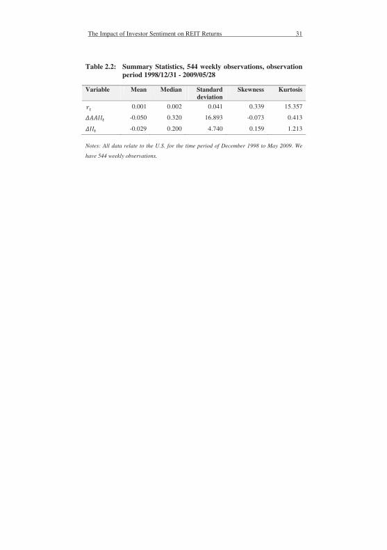
Table 2.2: Summary Statistics, 544 weekly observations,
observation period 1998/12/31 - 2009/05/28 .................31
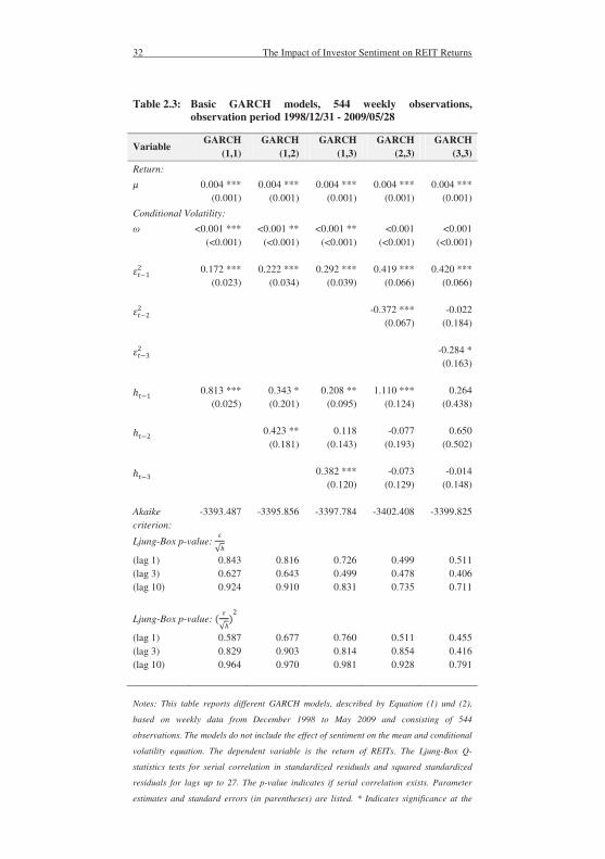
Table 2.3: Basic GARCH models, 544 weekly observations,
observation period 1998/12/31 - 2009/05/28 ..................32
Table 2.4: AAII sentiment threshold GARCH model , 544 weekly
observations, 1998/12/31 - 2009/05/28 .......................... 34
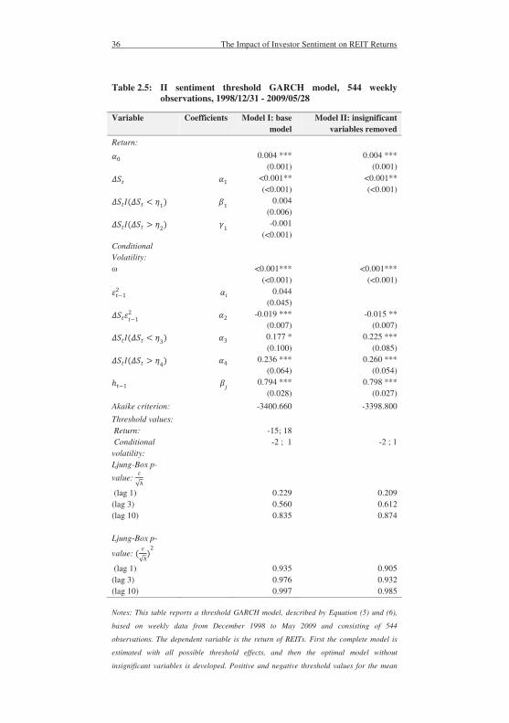
Table 2.5: II sentiment threshold GARCH model, 544 weekly observations, 1998/12/31 - 2009/05/28 .......................... 36
Table 3.1: Hypotheses, 627 weekly observations, observation period 1998/12/28 - 2010/12/27 ......................................60
Table 3.2: Summary Statistics, 627 weekly observations, observation period 1998/12/28 - 2010/12/27 .................. 61
Table 3.3: Investor sentiment and the financial crisis 2007, observation period 1998/12/28 - 2010/12/27 ....................62
Table 3.4: Hypotheses tests, 627 weekly observations, observation period 1998/12/28 - 2010/12/27 .................. 64
XX List of Tables
Table 4.1: Variable Definitions, 385 monthly observations,
observation period 1978/08 - 2010/08 ............ ........ . 89
Table 4.2: Summary Statistics, 385 monthly observations,
observation period 1978/08 - 2010/08 ...................... 90
Table 4.3: Results of the UCMs, 385 monthly observations,
observation period 1978/08 - 2010/08 ..................... 91
Table 4.4: Elasticities, 385 monthly observations, observation
period 1978/08 - 2010/08 .......................................... 92

Introduction 1
1 Introduction
In real estate capital markets several phenomena are observable that
are difficult to explain with the efficient market hypothesis. Property
companies typically offer market capitalizations that are smaller than
their net asset value (NAV), closed-end funds are usually traded at a
discount to their NAV and real estate investment trusts are often
mispriced. Attempts to explain these anomalies are at least
incomplete.
In financial markets, anomalies, such as excessive volatility of and
mean reversion in stock prices, are partly explained by the noise
trader theory. Black (1986) identifies noise traders to be responsible
for mispricing in financial markets. Noise traders suffer from
cognitive biases and disturb the market with their irrational trading.
A trigger for this is their reliance on investor sentiment, which is
defined by Baker and Wurgler (2007) as a prospect about the
development of future cash flows and investment risks based on
information that is not explained by fundamentals. This misguided
belief may be based, for example, on general market commentaries.
In what follows, we distinguish between investor sentiment and
consumer sentiment. Investor sentiment is specified as an aggregate
measurement of investors’ attitude towards prevalent market
conditions. It is usually determined as bullish, bearish or neutral.
A. Mathieu, Essays on the Impact of Sentiment on Real Estate Investments, Essays in Real Estate Research 9, DOI 10.1007/978-3-658-11637-8_1,© Springer Fachmedien Wiesbaden 2016

2 Introduction
Consumer sentiment, by contrast, reflects the perceptions individual
consumers have about the short-term and long-term prospects of the
economy in general and their personal financial situation in
particular.
De Long et al. (1990) first model the influence of noise trading on
assets considering the existence of arbitrage limits caused by noise
traders. In their model, noise traders act in concert on irrelevant
information, let prices deviate from fundamental values, and
introduce a systematic risk that is priced. This noise trader risk is
unpredictable as the beliefs of noise traders are uncertain. In the
short run, arbitrageurs face the risk that sentiment becomes more
extreme and prices deviate further from their fundamental values.
Arbitrageurs, who have to liquidate before the prices recover, risk to
lose money. The risk aversion and the short time horizon of
arbitrageurs in this model limit their willingness to take arbitrary
positions and impede the complete elimination of mispricing. Thus,
sentiment, respectively noise trading, has a persistent impact on
financial markets.
The importance of sentiment to understand the effectiveness of
financial markets is extensively studied in the financial literature.
However, until now only few studies exist investigating the impact
of sentiment on real estate markets or direct and indirect real estate
investments.
Introduction 3
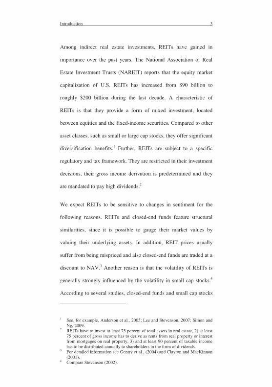
Among indirect real estate investments, REITs have gained in
importance over the past years. The National Association of Real
Estate Investment Trusts (NAREIT) reports that the equity market
capitalization of U.S. REITs has increased from $90 billion to
roughly $200 billion during the last decade. A characteristic of
REITs is that they provide a form of mixed investment, located
between equities and the fixed-income securities. Compared to other
asset classes, such as small or large cap stocks, they offer significant
diversification benefits.1 Further, REITs are subject to a specific
regulatory and tax framework. They are restricted in their investment
decisions, their gross income derivation is predetermined and they
are mandated to pay high dividends.2
We expect REITs to be sensitive to changes in sentiment for the
following reasons. REITs and closed-end funds feature structural
similarities, since it is possible to gauge their market values by
valuing their underlying assets. In addition, REIT prices usually
suffer from being mispriced and also closed-end funds are traded at a
discount to NAV.3 Another reason is that the volatility of REITs is
generally strongly influenced by the volatility in small cap stocks.4
According to several studies, closed-end funds and small cap stocks
1 See, for example, Anderson et al., 2005; Lee and Stevenson, 2007; Simon and Ng, 2009.
2 REITs have to invest at least 75 percent of total assets in real estate, 2) at least 75 percent of gross income has to derive as rents from real property or interest from mortgages on real property, 3) and at least 90 percent of taxable income has to be distributed annually to shareholders in the form of dividends.
3 For detailed information see Gentry et al., (2004) and Clayton and MacKinnon (2001).
4 Compare Stevenson (2002).
4 Introduction
are susceptible to the influence of investor sentiment.5 Since REITs
are to some degree similar to closed-end funds and related to small
cap stocks, it is likely that REIT returns and REIT return volatility
are also influenced by investor sentiment.
As REITs gain in importance and are often used as a hedging
instrument in a mixed-asset portfolio, it is important for shareholders
as well as for REIT managers to fully understand the return
generating process as well as the risk related to this investment class.
As investor sentiment is known to have significant influence in
financial markets, the relationship between sentiment and the real
estate capital market is important to be determined. Sentiment is a
factor that cannot be changed by actions of the REIT management or
by shareholders. Thus it is necessary to know how to handle this
factor and to anticipate its impact on the real estate capital market.
To provide an overall picture of the impact of sentiment on real
estate markets, it is helpful to consider not only indirect real estate
investments but also direct real estate investments. Direct real estate
markets are substantially different from financial markets. They are
characterized by heterogeneity, illiquidity, high transaction costs and
a lack of information.6 Unlike for stocks, no perfect substitutes exist
for properties. This makes a comparison of prices difficult. Further, a
5 Several studies investigate that closed-end funds and small cap stocks are influenced by investor sentiment, e.g. Lee et al. (1991), Chopra et al. (1993), Glushkov (2006).
6 Lin and Vandell (2007) identified these characteristics of real estate markets in their study.

Introduction 5
new home requires a high capital commitment and is not easily
resold quickly. We expect that these imperfections make real estate
markets susceptible to the influence of sentiment. In financial
markets, small imperfections, such as less liquidity, can cause more
activity of noise traders. Insecurity and risk combined with cognitive
biases let individuals rely on sentiment, when serves as an
orientation. As real estate markets are characterized by several
imperfections implying more risk and insecurity, they should be
even more prone to the influence of sentiment.
From a practitioner's point of view our work is of interest because
we illustrate for individuals as well as for real estate companies how
and to what degree sentiment influences direct real estate investment
decisions. A better understanding of the influencing factors of
investment decisions enables real estate companies to better
anticipate the demand and individuals to determine the optimal
investment date.
The purpose of the dissertation is to elucidate the impact of
sentiment on direct and indirect real estate investments. To achieve
this aim we compose three papers. In Paper one (Chapter two), we
analyze the impact of individual and institutional investor sentiment
on REIT returns. Our study applies a new methodology that enables
us to analyze simultaneously the impact of investor sentiment on
both the return and conditional return volatility of REITs. As bullish
and bearish sentiment may have a different impact on REIT returns
and REIT return volatility, we allow for asymmetries in our model.

6 Introduction
We expect that an increase in sentiment raises REIT returns, whereas
a decrease in sentiment may lower REIT returns. Further we
anticipate that both an increase and a decrease in investor sentiment
raise REIT return volatility.
In Paper two (Chapter three), we discuss a question that has so far
received no attention in the literature. We investigate the impact of
institutional investor sentiment on the formation of conditional
volatility and expected return both in a stable and an unstable market
environment. In particular, we compare an ordinary market situation
to the financial crisis that started in 2007. To capture different
investment classes, we analyze US Equity REIT returns, S&P 500
returns (large cap stocks) and NASDAQ returns (small cap stocks).
In an extreme market environment, we expect investor sentiment to
have a higher impact on the return generating process of REITs and
on REIT return volatility. Previous empirical tests of the impact of
investor sentiment have only considered ordinary market situations.
But noise traders enter the market in force in extreme market
situations. The financial crisis provides us a good opportunity to test
the behavior and the impact of noise traders under extreme market
conditions.
After a systematic analysis about the influence of investor sentiment
on indirect real estate investments, we turn in Paper three (Chapter
four) towards direct real estate markets. Our study is the first that
analyzes the impact of sentiment on residential real estate
investments. For this purpose, we investigate to what extent

Introduction 7
consumer sentiment and other key macroeconomic variables
influence the number of sales of new one-family homes in the U.S. If
households suffer from the same cognitive biases as financial
investors, consumer sentiment is bound to have an impact on their
decision process. We expect that a positive consumer sentiment
increases the number of new home sales, whereas a negative
consumer sentiment is attended by a decrease in sales of new homes.
In a positive market environment, employment is more stable and
households feel more confident to take on a large investment.
Negative consumer sentiment would indicate an unstable market
environment and would probably prevent households from investing
directly in real estate. The analysis is based on an unobserved
component model (UCM), which allows including observed
explanatory variables in a time series model along with unobserved
components, which absorb the impact of variables left out of the
study. This is important since it is not possible to obtain data for all
influencing variables or even to know what all the relevant variables
are, given the lack of a theory that relates sentiment to direct real
estate investments.
The remainder of the dissertation proceeds as follows. In Chapter
two we present Paper one. Using an asymmetric threshold GARCH
model, we test the impact of investor sentiment on the formation of
conditional volatility and expected return of REITs. We distinguish
between two different weekly sentiment indicators, one for
individual investor sentiment and one for institutional investor
8 Introduction
sentiment and use weekly US Equity REIT returns from December
1998 to May 2009.
Paper two is provided in Chapter three. In this study we use a
GARCH-M model to investigate the impact of institutional investor
sentiment on the formation of conditional volatility and expected
return both in an ordinary market situation and during the financial
crisis that started in 2007. We use a weekly sentiment indicator for
institutional investor sentiment, as well as weekly US Equity REIT
returns, S&P 500 returns and NASDAQ returns from December
1998 to December 2010.
In Chapter four we introduce Paper three. While Paper one and two
concentrate on the impact of investor sentiment on indirect real
estate markets, Paper three considers direct real estate markets.
Using an unobserved component model (UCM) we investigate the
impact of several macroeconomic influencing factors, particularly
consumer sentiment, on the number of new one-family home sales in
the U.S. We use monthly U.S. data from August 1978 to August
2010. Five different explanatory variables are considered: consumer
sentiment, the mortgage rate, real estate loans, the inflation rate and
the disposable personal income.
Chapter five summarizes the results.
The Impact of Investor Sentiment on REIT Returns 9
2 The Impact of Investor Sentiment on
REIT Returns
Co-authors of this chapter are N. Rottke and J. Zietz.
2.1 Introduction
The behavior of real estate investment trust (REIT) returns and REIT
return volatility is a key topic in the real estate literature. Various
studies concentrate on the return generating process of REITs. Chui
et al. (2003), for instance, examine the cross-sectional determinants
of expected REIT returns. Hsieh and Peterson (1997) find that risk
premiums on equity REITs are related to their market capitalization
and the book to market ratio. Clayton and MacKinnon (2003)
analyze the link between REIT prices and the value of direct real
estate owned by REITs.
Other papers focus on the volatility of REIT returns. Stevenson
(2002) examines volatility spillovers of REITs. Devaney (2001)
investigates the relationship between REIT volatility and interest
rates. Cotter and Stevenson (2004) analyze the volatility dynamics in
daily equity REIT returns and Hung and Glascock (2010) studies
momentum returns in REITs.
A. Mathieu, Essays on the Impact of Sentiment on Real Estate Investments, Essays in Real Estate Research 9, DOI 10.1007/978-3-658-11637-8_2,© Springer Fachmedien Wiesbaden 2016
10 The Impact of Investor Sentiment on REIT Returns
Several stylized facts have emerged thus far. First, according to
several studies REIT prices deviate from net asset values (for
example, Gentry et al., 2004; Clayton and MacKinnon, 2001).
Second, REITs provide a form of mixed investment, located between
equities and the fixed-income sector. They are unique in that they
offer significant diversification benefits over other asset classes, such
as small or large cap stocks and bonds.7 Third, following Stevenson
(2002) the volatility of REITs is generally influenced more strongly
by volatility in small cap stocks and in firms classified as value
stocks.
These stylized facts raise the question if REITs - as closed-end-funds
and small cap stocks - are exposed to the influence of investor
sentiment. There appear to be few studies that relate explicitly to
REITs. Most focus on small caps or closed-end funds. For example,
Lee et al. (1991) examine whether changes in closed-end fund
discounts are caused by market sentiment. Glushkov (2006)
investigates whether small cap and more volatile stocks with low
dividend yields are influenced by sentiment.
REITs are similar to closed-end funds, since it is possible to gauge
the market value of REITs by valuing the underlying assets. Further,
REIT prices usually suffer from being undervalued and closed-end
funds are traded at a discount to NAV. The basic characteristic that
7 See, for example, Anderson et al., 2005; Lee and Stevenson, 2007; Simon and Ng, 2009.
The Impact of Investor Sentiment on REIT Returns 11
distinguishes REITs from closed-end funds is the illiquid asset that
REITs own. Since REITs are similar to closed-end funds in terms of
their structure, and their volatility is influenced by small cap stock
volatility, REITs are probably influenced by market sentiment. To
what extent that is true, is the focus of this study.
More precisely, the current paper extends the literature on REIT
returns and volatility by considering the impact of investor sentiment
on REIT returns and volatility. Our main findings suggest that
individual investor sentiment is a significant factor in explaining
REIT returns and REIT return volatility. We can also identify
asymmetric sentiment threshold values for both the return and the
conditional volatility parts of the model. REIT returns increase in
bullish sentiment stages, whereas bearish sentiment has no impact on
the returns. The volatility increases in both sentiment stages, but bad
news tends to have a larger effect.
The remainder of the study proceeds as follows. Section two gives
an overview of the literature on investor sentiment as it is relevant to
REITs. Section three describes the data and the different empirical
models that are estimated. Section four discusses the empirical
results and section five concludes with a summary of the study’s
most important results.

12 The Impact of Investor Sentiment on REIT Returns
2.2 Literature Review
The idea to analyze REIT returns and REIT return volatility in
different sentiment stages is based on the noise trader theory (for
example, Black, 1986; DeLong et al., 1990). Noise traders seem to
act primarily in extreme sentiment stages. Accordingly, extreme
sentiment stages may cause changes in REIT returns and REIT
return volatility.
The aim of the noise trader theory has been to find explanations for
market anomalies, such as excessive volatility of and mean reversion
in stock prices, the small firm effect and under- or overreaction of
stock prices. These anomalies are difficult to explain with the
efficient market hypothesis.
The empirical evidence suggests that not all investors buy and hold
the market portfolio as recommended by economists. Instead,
according to Lease et al. (1974) some investors pick their stocks by
their own research and do not diversify their portfolio. Black (1986)
ascertains that these investors seem to form their beliefs on anything
but fundamentals and act irrationally on noise as if it were profitable
information. In other words, noise traders’ decisions to buy, sell, or
hold an asset are based on a “noisy” signal. Kahneman and Tversky
(1974) provide a multiplicity of possible cognitive biases in their
studies, such as anchoring, representativeness or availability that try
to explain reasons for the behavior of these investors.

The Impact of Investor Sentiment on REIT Returns 13
Early studies (Friedman, 1953; Fama, 1965) attach no importance to
the existence of so-called noise traders.8 They assume that an
investor trading on anything but fundamentals would be forced out
of the market by arbitrageurs. This would let prices return to their
fundamental values. However, continuing market anomalies
challenge the efficient market hypothesis.
DeLong et al. (1990) first model the influence of noise trading on
assets considering the existence of arbitrage limits caused by noise
traders. In their model, noise traders act in concert on irrelevant
information, let prices deviate from fundamental values, and
introduce a systematic risk that is priced. This noise trader risk is
unpredictable as the beliefs of noise traders are uncertain. In the
short run, arbitrageurs face the risk that sentiment becomes more
extreme and prices deviate further from their fundamental values.
Arbitrageurs, who have to liquidate before the prices recover, risk to
lose money. The risk aversion and the short time horizon of
arbitrageurs in this model limit their willingness to take arbitrary
positions and impede the complete elimination of mispricing.
Investor sentiment influences the behavior of noise traders: in
positive (negative) sentiment stages noise traders become extremely
optimistic (pessimistic) and buy (sell) more of the asset. In summary,
extreme sentiment stages let noise traders act and their trading has an
persistent impact on returns and raises return volatility.
8 Kyle (1985) first uses the term “noise trader” in their study.

14 The Impact of Investor Sentiment on REIT Returns
Noise traders react asymmetrically in positive and negative
sentiment stages. Bad news tends to have a larger negative effect on
the return and the conditional volatility than good news has a
positive effect. According to Barberis and Huang (2001) reasons for
these effects are the loss aversion and the narrow framing of
individuals. Loss aversion is the tendency of individuals to be more
sensitive to losses than to gains. Narrow framing indicates the bias of
individuals to focus on narrowly defined gains and losses.
The relationship between investor sentiment and noise trading is well
investigated for closed-end funds and small cap stocks, but there has
been little research for REITs. The question is whether and to what
extent REITs are also exposed to the influence of investor sentiment.
This is an important question because REITs have historically been
viewed as providing investors protection during market downturns.
In the literature, noise traders have not yet been exactly identified as
individual or institutional investors. DeLong et al. (1990) assume
that individual investors are more likely to be noise traders because
they tend to be less sophisticated and more prone to cognitive biases.
According to Weiss (1989), closed-end fund shares are primarily
held by individual investors. Following up on Weiss, Lee et al.
(1991) find a possible explanation for the closed-end fund puzzle
presented by Zweig (1973), which is one of the most persistent
puzzles related to the efficient market hypothesis. Lee et al. (1991)
discover that changes in closed-end fund discounts are highly
correlated with returns of small stocks that are mainly held by

The Impact of Investor Sentiment on REIT Returns 15
individual investors and infer that the previously unexplained
discounts are caused by market sentiment. Swaminathan (1996) and
Neal and Wheatley (1998) suggest that closed-end fund discounts
predict small firm returns. Glushkov (2006) reports that more
sentiment sensitive stocks have higher individual ownership and
Brown (1999) investigates the price volatility of closed-end funds
and finds a close relation to unusual levels of sentiment.
Chen et al. (1993) and Brown and Cliff (2005) do not support the
conventional wisdom that sentiment primarily affects individual
investors and small stocks. Hughen and McDonald (2005) further
show that the order-flow imbalances of small investors do not cause
large changes in fund discounts. Instead, fluctuations in fund
discounts are strongly correlated with trading activity of institutional
investors that have enough market power to strongly affect prices.
REIT institutional ownership is quite high. Clayton and MacKinnon
determine that, during the 1990-1998 period, institutional ownership
in REITs increased to over fifty percent. This stands in contrast to
closed-end funds, which are mainly held by individual investors. It
is, therefore, not clear if an indicator for individual or institutional
investor sentiment is better suited to measure the influence of
sentiment on REITs. To allow for this fact, we use both an individual
investor sentiment measure and an institutional investor sentiment
measure. The analysis will show which measure is more appropriate.

16 The Impact of Investor Sentiment on REIT Returns
Although there is a growing number of theoretical and empirical
studies that investigates the role of investor sentiment in financial
markets (for example, DeLong et al., 1990, Lee et al., 1991, Brown
and Cliff, 2004), only few have focused on the real estate sector. Lin
et al. (2009), for example, find that sentiment has a significant
positive impact on REIT returns. Clayton and MacKinnon (2001)
report that the discount to NAV in REIT pricing is caused by noise.
Falzon (2002) suggests a strong relationship between REITs and
small capital stocks, and finds the relationship is especially strong
with small capital value stocks. The relationship between sentiment
and REIT return volatility appears to be unexplored so far.
To investigate the relationship between REITs and sentiment, we
estimate several generalized autoregressive conditional
heteroscedasticity (GARCH) models, introduced by Bollerslev
(1986), with sentiment as the key explanatory variable. We
distinguish two sentiment indicators, one for individual investors and
one for institutional investors. For each indicator, we test for
nonlinearities that may arise from threshold effects. Not every
movement in the sentiment index may have a proportionate impact
on REIT return or volatility; only sentiment changes beyond a
certain critical value may have an impact. Our study is the first one
that analyses sentiment threshold values. Furthermore, we are the
first to allow the impact of positive and negative sentiment on REIT
return and volatility to be asymmetric. In studies about stocks, such
The Impact of Investor Sentiment on REIT Returns 17
asymmetries are found to be important (for example, Barberis and
Huang, 2001, Kirchler, 2009).
2.3 Data and Methodology
In this section we describe the data and several GARCH models that
we estimate to analyze the impact of individual and institutional
investor sentiment on REIT returns and REIT return volatility.
2.3.1 Data
The data consist of US equity REIT total returns and two different
US sentiment indicators. The REIT returns are derived as ,
where is the stock price of the REITs.
The first sentiment indicator is based on a survey regularly
conducted by the American Association of Individual Investors
(AAII) since July 1987. The association asks each week a random
sample of its members where they think the stock market will be in
six months. The responses, which are coded as up, down or the
same, are interpreted as bullish, bearish or neutral market sentiments.
Within the observation period, the responses are on average 39
percent bullish, 30 percent bearish and 31 percent neutral. Since the
association asks mainly individuals, this indicator is often interpreted
as a measure of individual investor sentiment.
18 The Impact of Investor Sentiment on REIT Returns
The second sentiment measure relies on the survey of Investor
Intelligence (II) founded in 1963. The association studies over a
hundred independent market newsletters every week and assesses
each author’s current stance on the market: bullish, bearish or
waiting for a correction. On average, 48 percent of the newsletters
expect future market movements to be bullish and 30 percent expect
bearish market movements within the observation period. Since
many of the authors of these market newsletters are market
professionals, this indicator is interpreted as a measure of
institutional investor sentiment. For both indicators, the percentage
of bullish investors minus the percentage of bearish investors (bull-
bear spread) is used to identify the market sentiment.
All variables consist of 544 observations and are observed weekly
from December 31, 1998 to May 28, 2009. The REIT data are
derived from the SNL Financial database and the data of the two
sentiment indicators are from Thomson Reuters Datastream.
2.3.2 The GARCH Model without Sentiment
We first estimate a GARCH model without sentiment to provide a
basis of comparison for the following models. The return equation of
the model takes the form
(1)

The Impact of Investor Sentiment on REIT Returns 19
where is the weekly return on US equity REITs, a time invariant
constant, and a disturbance term. The conditional volatility
equation of the model is given in standard format as
,
where is the conditional volatility of US equity REIT returns.
2.3.3 The Sentiment Threshold GARCH Model
The base model consisting of Equations (1) and (2) is expanded by
allowing for threshold values for the sentiment variable ( ). We
allow for asymmetric reactions with positive and negative threshold
values. The return equation of the model including investor
sentiment and asymmetry effects takes the form
where is an indicator variable, which is unity if
and zero if . The scalar denotes the threshold value for
negative changes in sentiment. is an indicator variable,
which is unity if and zero if . is the threshold
value for positive changes in sentiment. The conditional volatility
equation of the model is given as

20 The Impact of Investor Sentiment on REIT Returns
where and are indicator variables, which are
unity for the specified conditions and zero otherwise.
The zero/one indicator variables (I) in the mean and the conditional
volatility equations allow for asymmetric reactions to changes in the
direction and magnitude of the sentiment variable. The rationale for
the asymmetric terms is simple: they allow investors to react
differently to changes in bullish and bearish sentiment. This is in line
with the finance literature (for example, Glosten et al., 1993; Backus
and Gregory, 1993), which find bearish sentiment to have a larger
impact than periods of bullish sentiment.
The estimation of threshold values for both the mean return equation
and the conditional volatility equation enables us to compare the
relative sentiment sensitivity of the return and the conditional
volatility. The lower the sentiment threshold value is the higher is
the sentiment sensitivity. We expect the conditional volatility to have
lower threshold values compared to the returns of REITs, as
relatively small changes in sentiment may cause buy/sell actions of
investors and thus increase conditional volatility. The return however
may be only affected by more severe changes in investor sentiment.
2.4 Empirical Results
This section presents the empirical evidence on the impact of
sentiment on mean returns and conditional volatility.
The Impact of Investor Sentiment on REIT Returns 21
2.4.1 Augmented Dickey-Fuller Test and KPSS Test
Table 2.1 shows the results of the augmented Dickey-Fuller (ADF)
tests for a unit root. Stationarity requires a rejection of the null
hypothesis of a unit root. This is the case if the p-value of the ADF
test statistic is lower than the significance level = 1%. The ADF
test with constant reveals that all variables are stationary. We also
estimate the KPSS test, which has the null hypothesis of stationarity.
The null hypothesis is rejected if the critical value of 0.739 is
exceeded. This is the case for and . The variables
and are stationary.
Since both tests do not have the same conclusion, we use in level
form and for both sentiment indicators we employ first differences.
This ensures that all variables are stationary. Furthermore, it makes
economic sense to use the first differences of the sentiment variables
because changes in the sentiment variable are of primary interest.
2.4.2 Summary Statistics
As reported in Table 2.2 and measure changes in
investor sentiment and therefore capture innovations in individual
and institutional investor sentiment. The mean of both sentiment
indicators are small and negative over the sample period. has a
small, positive mean and displays a skewed, leptokurtic pattern.
and show a skewed and platykurtic distribution. The
relatively high standard deviation - particularly for -indicates

22 The Impact of Investor Sentiment on REIT Returns
that the low mean is due to the fact that positive and negative
changes in sentiment are offsetting.
2.4.3 The GARCH Model without Sentiment
First, we estimate several basic GARCH models, as described by
Equations (1) and (2). The coefficient estimates are reported in Table
2.3. For the purpose of comparison these models exclude sentiment
variables in the mean and conditional volatility equation. Across the
different GARCH models, most of the estimated GARCH
coefficients are significant. The analysis shows that GARCH effects
exist in both REIT returns and REIT return volatility.
To compare the different models and to select the most appropriate
one, we use the Akaike information criterion (AIC). It indicates that
a simple GARCH (2,3) model is the most appropriate one for the
data. For all GARCH models, the Ljung-Box p-values indicate that
no serial correlation exists in either the standardized residuals or the
squared standardized residuals. That means the null hypothesis of no
autocorrelation cannot be rejected. The models fit the data well.
2.4.4 The Sentiment Threshold GARCH Model
Next, we include investor sentiment in both the mean return and
conditional volatility equation of our model. Our purpose is to detect
asymmetries in the impact of sentiment as well as to investigate if
certain sentiment threshold values exist. Accordingly, we use a
GARCH model that allows for positive and negative sentiment

The Impact of Investor Sentiment on REIT Returns 23
threshold values. We estimate two models, one with an indicator for
individual investor sentiment (AAII) and one with an institutional
investor sentiment indicator (II).
AAII Sentiment Thresholds
The first model includes individual investor sentiment as an
explanatory variable in the mean and conditional volatility equations,
as described by Equations (3) and (4). The coefficient estimates are
reported in Table 2.4. We start with the estimation of the complete
model with all possible threshold effects. The results show primarily
significant coefficients, indicating a widespread impact of individual
investor sentiment on REIT returns. We estimate further models,
which exclude insignificant variables to improve the Akaike
information criterion (AIC) and get the optimal model.
For all three models of Table 2.4, the Ljung-Box p-values suggest
the absence of serial correlation in the standardized and squared
standardized residuals. We find that Model III is most suitable for
the data, since it has the lowest AIC value. To identify the threshold
values for the mean and the conditional volatility equations, we
estimate values in the range from 0 to 30 and from 0 to -30. These
ranges for the threshold values are determined on the basis of the
kernel density function of the sentiment changes in Figure 2.1.
Approximately at the points +30 and -30 are inflection points of the
graph, indicating the maximal respectively minimal range for the
threshold values.

24 The Impact of Investor Sentiment on REIT Returns
The threshold values for the mean equation (-21; 25) and for the
conditional volatility (-3; 8) equation do not differ between the three
models. The relatively small threshold values of the conditional
volatility equation suggest that even small changes in sentiment
influence the conditional volatility of REITs. Nearly every positive
or negative news seems to bias the trading behavior of REIT
investors. REIT returns however are only affected by relatively
strong changes in individual investor sentiment.
In the mean equation of the preferred Model III, positive and
negative changes in sentiment have almost no impact at the extreme
ends of the distribution of the sentiment variable, as the return is not
affected by changes in sentiment that are smaller than the negative
threshold value (-21) or larger than the positive threshold value
(25).9 If changes in sentiment are greater than the negative threshold
value (-21) or smaller than the positive threshold value (25), the
return increases approximately by 0.001 units. By contrast, we find
that sentiment has a significant impact on volatility. Bullish changes
in sentiment that exceed the positive threshold value result in
statistically significant increases in volatility; in particular, the
volatility changes approximately by 0.106. Bearish changes in
sentiment that fall below the negative threshold value let the
volatility increase by approximately 0.272. This finding is in line
with Glosten et al. (1993) who report that the magnitude of the
9 The addition of and respectively of and is approximately zero.

The Impact of Investor Sentiment on REIT Returns 25
change in market volatility is greater in bearish than in bullish
sentiment stages.
In summary, we can say that individual investor sentiment does
indeed capture the influence of market sentiment on REIT returns
and REIT return volatility. In the mean equation, we find only a
small influence of sentiment. In the conditional volatility equation,
we detect an asymmetric impact. In particular, the negative threshold
value is smaller and the negative sentiment has a stronger impact on
the conditional volatility of REITs than the positive one.
II Sentiment Thresholds
We estimate a sentiment threshold GARCH model with institutional
investor sentiment as the explanatory variable in the mean and
conditional volatility equations (Equations (3) and (4)). The
estimates of the coefficients are reported in Table 2.5. In Model I, we
estimate the complete model with all possible threshold effects.
Some of the coefficients are insignificant, which we remove in
Model II from the mean and volatility equation. The Ljung-Box p-
values report no serial correlation for either the standardized
residuals or the squared standardized residuals for the two models.
The models fit the data as serial correlation is effectively absent. We
find again that a GARCH (1,1) is most suitable for the data.
Threshold values are tested for the mean and the conditional
volatility equations in the range from 0 to 20 and from 0 to -20. The
ranges for the threshold values are determined on the basis of the

26 The Impact of Investor Sentiment on REIT Returns
kernel density function of the sentiment changes (Figure 2.2). In
Model I the threshold values for the mean equation are -15 and 18,
but the corresponding coefficients are not significant. Therefore, we
remove the insignificant variables in Model II. Changes in sentiment
without consideration of threshold effects raise the return by
approximately 0.001. Furthermore, we find that the threshold values
of the conditional volatility equation are smaller compared to the
model with the individual investor sentiment indicator, namely -2
and 1. In Model II, a one unit change in bullish sentiment raises the
volatility approximately by 0.24510. Bearish changes in sentiment let
the volatility increase by approximately 0.21011. These findings
contradict the results of Lee et al, who detect a negative correlation
between changes in investor sentiment and stock market volatility. It
is apparent that the two sentiment indicators, described in
Table 2.4 and Table 2.5, behave differently. The indicator of
individual investor sentiment fits the data better according to the
information criteria and provides more reasonable results. Since
investors are risk averse, bearish changes in sentiment should have a
stronger impact on conditional volatility than bullish changes in
sentiment; this is only the case for the individual investor sentiment
indicator. The results are interesting as institutional investors
primarily invest in REITs. Therefore, one would expect the indicator
10 The value 0.245 is derived from the addition of and 11 The value 0.240 is derived from the addition of and

The Impact of Investor Sentiment on REIT Returns 27
for institutional investor sentiment to be the more appropriate
explanatory variable for REIT returns and REIT return volatility.
Overall, our results contradict the conventional wisdom that only
small stocks are affected by noise trading (Baker and Wurgler,
2007). The results are, however, in line with the findings of Brown
and Cliff (2004), which do not support the conventional view. REITs
also seem to be sensitive to sentiment changes although they are
primarily held by institutions and not individuals. To measure the
influence of sentiment on REITs, the indicator for individual
investor sentiment is the most appropriate.
2.5 Conclusions
The purpose of this study has been to analyze the influence of
investor sentiment on REIT returns and REIT return volatility. This
is the first study to investigate if the impact of sentiment on REIT
returns and REIT return volatility is asymmetric. In studies about
stocks such asymmetries are found (for example, Barberis, N. and
Huang, M., 2001; Kirchler, M., 2009). This is also the first study to
analyze if nonlinear effects of the threshold type exist for sentiment.
In our analysis we use two different weekly sentiment indicators, one
for individual investor sentiment (AAII) and one for institutional
investor sentiment (II), as well as weekly US Equity REIT returns
from December 1998 to May 2009. We apply a GARCH framework

28 The Impact of Investor Sentiment on REIT Returns
to test the influence of investor sentiment on REIT returns and
conditional volatility. We find that including a sentiment variable as
an explanatory variable into a basic GARCH model improves the fit.
The same applies to including threshold effects for the sentiment
variables. For the indicator of individual investor sentiment, we
identify a small positive influence on REIT returns. In the
conditional volatility equation, we detect some weak asymmetry.
Negative sentiment changes have a stronger impact on the
conditional volatility of REITs. However, in bullish and bearish
sentiment stages, sentiment changes that exceed the threshold values
tend to increase volatility.
The inclusion of institutional investor sentiment in the model leads
to inferior models compared to the analysis with individual investor
sentiment. In the mean equation, we find again a small positive
influence of institutional investor sentiment on REIT returns. In the
volatility equation, positive and negative sentiment changes raises
volatility by a similar magnitude. Sentiment changes that fall below
the positive threshold value respectively exceed the negative
threshold value have a negative impact on the conditional volatility.
In summary, we ascertain that REIT returns and REIT return
volatility are influenced by investor sentiment. The indicator for
individual investor sentiment is the most appropriate indicator for
REITs. The impact of individual investor sentiment on REIT returns
and REIT return volatility is asymmetric: bearish sentiment has a
stronger impact on the volatility of REITs. This is consistent with

The Impact of Investor Sentiment on REIT Returns 29
Barberis and Huangs’ (2001) finding that investors are loss averse
and focus on narrowly defined gains and losses. Furthermore, the
influence of sentiment on the conditional volatility is higher than on
the mean return, as the corresponding threshold values are smaller
for the conditional volatility equation.
Sentiment is, contrary to conventional wisdom, not an individual
investor problem that only affects small capitalization stocks and
closed-end funds. It also affects REITs.

30 The Impact of Investor Sentiment on REIT Returns
2.6 Appendix for Chapter Two
Table 2.1: Augmented Dickey-Fuller tests and KPSS tests, 544 weekly observations, observation period 1998/12/31 - 2009/05/28
Variable ADF test KPSS test
0.002 (14) 0.318
0.004 (4) 0.009
< 0.001 (6) 2.439
0.001 (13) 0.009
< 0.001 (1) 1.062
< 0.001 (15) 0.015
Notes: This table provides augmented Dickey-Fuller (ADF) tests and KPSS tests for the
return, sentiment indices, changes in returns and changes in sentiment indices. The ADF
test statistic is calculated with a constant, no time trend is used, the p-values are shown and
the optimal lag choice is in parentheses. The KPSS test is done without time trend and the
critical values at different significance levels are: 10% (0.347), 5% (0.463), 2.5% (0.574),
1% (0.739). The weekly data consists of 544 observations from December 1998 to May
2009.
The Impact of Investor Sentiment on REIT Returns 31
Table 2.2: Summary Statistics, 544 weekly observations, observation period 1998/12/31 - 2009/05/28
Variable Mean Median Standard deviation
Skewness Kurtosis
0.001 0.002 0.041 0.339 15.357
-0.050 0.320 16.893 -0.073 0.413
-0.029 0.200 4.740 0.159 1.213
Notes: All data relate to the U.S. for the time period of December 1998 to May 2009. We
have 544 weekly observations.
32 The Impact of Investor Sentiment on REIT Returns
Table 2.3: Basic GARCH models, 544 weekly observations, observation period 1998/12/31 - 2009/05/28
Variable GARCH
(1,1) GARCH
(1,2) GARCH
(1,3) GARCH
(2,3) GARCH
(3,3)
Return:
0.004 *** (0.001)
0.004 *** (0.001)
0.004 *** (0.001)
0.004 *** (0.001)
0.004 *** (0.001)
Conditional Volatility:
<0.001 *** (<0.001)
<0.001 ** (<0.001)
<0.001 ** (<0.001)
<0.001 (<0.001)
<0.001 (<0.001)
0.172 *** (0.023)
0.222 *** (0.034)
0.292 *** (0.039)
0.419 *** (0.066)
0.420 *** (0.066)
-0.372 *** (0.067)
-0.022 (0.184)
-0.284 * (0.163)
0.813 *** (0.025)
0.343 * (0.201)
0.208 ** (0.095)
1.110 *** (0.124)
0.264 (0.438)
0.423 ** (0.181)
0.118 (0.143)
-0.077 (0.193)
0.650 (0.502)
0.382 *** (0.120)
-0.073 (0.129)
-0.014 (0.148)
Akaike criterion:
-3393.487
-3395.856
-3397.784
-3402.408
-3399.825
Ljung-Box p-value:
(lag 1) (lag 3) (lag 10)
0.843 0.627 0.924
0.816 0.643 0.910
0.726 0.499 0.831
0.499 0.478 0.735
0.511 0.406 0.711
Ljung-Box p-value:
(lag 1) (lag 3) (lag 10)
0.587 0.829 0.964
0.677 0.903 0.970
0.760 0.814 0.981
0.511 0.854 0.928
0.455 0.416 0.791
Notes: This table reports different GARCH models, described by Equation (1) und (2),
based on weekly data from December 1998 to May 2009 and consisting of 544
observations. The models do not include the effect of sentiment on the mean and conditional
volatility equation. The dependent variable is the return of REITs. The Ljung-Box Q-
statistics tests for serial correlation in standardized residuals and squared standardized
residuals for lags up to 27. The p-value indicates if serial correlation exists. Parameter
estimates and standard errors (in parentheses) are listed. * Indicates significance at the

The Impact of Investor Sentiment on REIT Returns 33
10% level, ** indicates significance at the 5% level, *** indicates significance at the 1%
level.

34 The Impact of Investor Sentiment on REIT Returns
Table 2.4: AAII sentiment threshold GARCH model, 544 weekly observations, 1998/12/31 - 2009/05/28
Variable Coefficient Model I: base model
Model II: insignificant
variables removed
Model III: more insignificant
variables removed
Return:
0.002 * (0.001)
0.002 ** (0.001)
0.002 ** (0.001)
<0.001*** (<0.001)
<0.001*** (<0.001)
<0.001*** (<0.001)
<-0.001 *** (<0.001)
<-0.001*** (<0.001)
<-0.001*** (<0.001)
<-0.001 ** (<0.001)
<-0.001 ** (<0.001)
<-0.001** (<0.001)
Conditional Volatility:
<0.001** (<0.001)
<0.001** (<0.001)
<0.001** (<0.001)
-0.035 (0.025)
0.004* (0.002)
0.004 (0.002)
0.254*** (0.061)
0.223 *** (0.047)
0.272 *** (0.032)
0.128 *** (0.047)
0.107 ** (0.052)
0.106 *** (0.034)
0.881*** (0.014)
0.863 *** (0.016)
0.870 *** (0.014)
Akaike criterion:
-3411.896 -3412.874 -3412.621
Threshold values: Return: Conditional volatility:
-21; 25 -3 ; 8
-21; 25
-3; 8
-21;25 -3 ; 8
Ljung-Box p-value:
(lag 1) (lag 3) (lag 10)
0.558 0.409 0.800
0.693 0.464 0.870
0.770 0.513 0.922
Ljung-Box p-value:
(lag 1) (lag 3) (lag 10)
0.197 0.168 0.566
0.404 0.705 0.913
0.443 0.538 0.894
Notes: This table reports a threshold GARCH model, described by Equation (5) und (6),
based on weekly data from December 1998 to May 2009 and consisting of 544
observations. The dependent variable is the return of REITs. First the complete model is
estimated with all possible threshold effects, and then the optimal model without
insignificant variables is developed. Positive and negative threshold values for the mean

The Impact of Investor Sentiment on REIT Returns 35
and the conditional volatility equations are reported. The Ljung-Box Q-statistics tests for
serial correlation in standardized and squared standardized residuals for lags up to 27. The
p-value indicates if serial correlation exists. Estimates and standard errors (in parentheses)
are listed. *Indicates significance at the 10% level, **indicates significance at the 5% level,
***indicates significance at the 1% level.
36 The Impact of Investor Sentiment on REIT Returns
Table 2.5: II sentiment threshold GARCH model, 544 weekly observations, 1998/12/31 - 2009/05/28
Variable Coefficients Model I: base model
Model II: insignificant variables removed
Return:
0.004 *** (0.001)
0.004 *** (0.001)
<0.001** (<0.001)
<0.001** (<0.001)
0.004 (0.006)
-0.001 (<0.001)
Conditional Volatility:
<0.001*** (<0.001)
<0.001*** (<0.001)
0.044(0.045)
-0.019 ***(0.007)
-0.015 ** (0.007)
0.177 *(0.100)
0.225 *** (0.085)
0.236 *** (0.064)
0.260 *** (0.054)
0.794 ***(0.028)
0.798 *** (0.027)
Akaike criterion: -3400.660 -3398.800
Threshold values: Return: Conditional volatility:
-15; 18 -2 ; 1
-2 ; 1
Ljung-Box p-
value:
(lag 1) (lag 3) (lag 10)
0.229 0.560 0.835
0.209 0.612 0.874
Ljung-Box p-
value:
(lag 1) (lag 3) (lag 10)
0.935 0.976 0.997
0.905 0.932 0.985
Notes: This table reports a threshold GARCH model, described by Equation (5) und (6),
based on weekly data from December 1998 to May 2009 and consisting of 544
observations. The dependent variable is the return of REITs. First the complete model is
estimated with all possible threshold effects, and then the optimal model without
insignificant variables is developed. Positive and negative threshold values for the mean

The Impact of Investor Sentiment on REIT Returns 37
and the conditional volatility equations are reported. The Ljung-Box Q-statistics tests for
serial correlation in standardized and squared standardized residuals for lags up to 27. The
p-value indicates if serial correlation exists. Estimates and standard errors (in parentheses)
are listed. *Indicates significance at the 10% level, **indicates significance at the 5% level,
***indicates significance at the 1% level.

38 The Impact of Investor Sentiment on REIT Returns
Figure 2.1: Kernel density function of AAII sentiment indicator
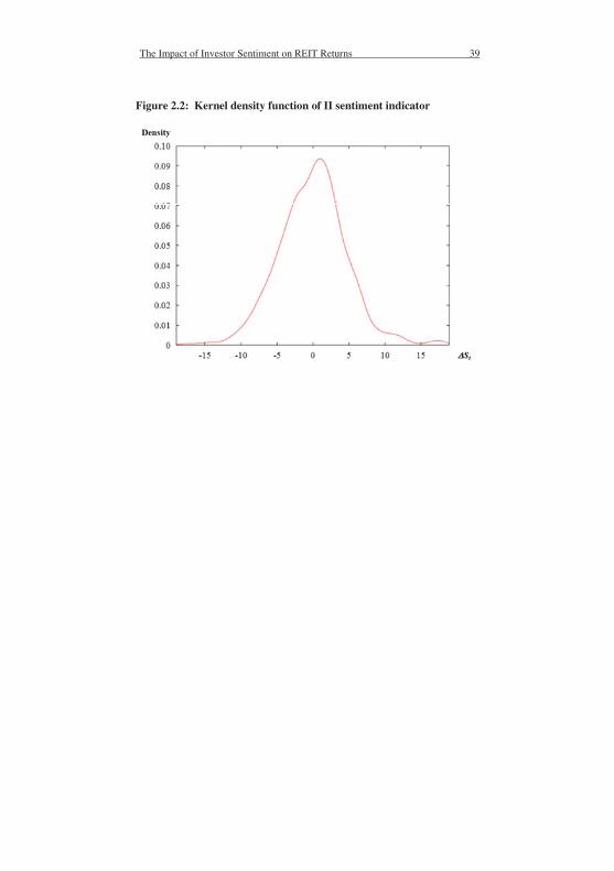
The Impact of Investor Sentiment on REIT Returns 39
Figure 2.2: Kernel density function of II sentiment indicator

40 REITs and Non-REITs during the Financial Crisis
3 Investor Sentiment and the Return
and Volatility of REITs and Non-
REITs during the Financial Crisis
Co-authors of this chapter are N. Rottke and J. Zietz.
3.1 Introduction
The participation of noise traders in financial markets has different
effects for returns and return volatility. Noise traders participate in
the market is based on an external, noisy signal that conveys no
information about fundamentals. Investor sentiment is such a signal.
Sentiment reflects the optimism or pessimism of the market and does
not need to be completely rational. The more extreme the sentiment
is, the more noise traders act in the market; their trading lets prices
deviate from their fundamental values. This deviation is persistent
and introduces a new kind of risk - the noise trader risk (Shleifer and
Summers, 1990, Sias et al., 2001, De Long et al., 1989).
The current paper extends the literature on sentiment by considering
the impact of institutional investor sentiment on returns and
conditional volatility of different asset classes in an unstable market
environment. We use a GARCH-M model to identify to what extent
returns and conditional volatilities are influenced by investor
A. Mathieu, Essays on the Impact of Sentiment on Real Estate Investments, Essays in Real Estate Research 9, DOI 10.1007/978-3-658-11637-8_3,© Springer Fachmedien Wiesbaden 2016

REITs and Non-REITs during the Financial Crisis 41
sentiment. To capture different investment classes, we analyze US
Equity REIT returns, S&P 500 returns (large cap stocks) and
NASDAQ returns (small cap stocks). As noise traders are more
active in extreme sentiment stages, we allow the impact of sentiment
on returns and return volatility to be different during the financial
crisis that started in 2007 than during tranquil times.
Our main findings suggest that for REIT and S&P 500 returns the
impact of investor sentiment on returns and return volatility is higher
during the financial crisis than in a tranquil market environment.
Further, the impact of return volatility on contemporaneous REIT
and S&P 500 returns is significantly higher during the financial
crisis. Generally, REIT returns and S&P 500 returns behave
similarly with regard to investor sentiment. NASDAQ returns are
influenced by market sentiment at large, with no particular
difference observable during the financial crisis.
The remainder of the study proceeds as follows. Section two
specifies the theoretical background of the study. Section three
describes the data, the methodology and the individual hypotheses.
Section four discusses the empirical results and section five
concludes with a summary of the study’s most important results.

42 REITs and Non-REITs during the Financial Crisis
3.2 Theoretical Background
Several theoretical models have been developed to show that
irrational trading has a long term impact on asset prices (Hirshleifer
et al., 2006, Dumas et al., 2005). De Long et al. (1990) (DSSW
hereafter) first model theoretically the influence of noise trading on
expected returns and conditional volatility. In their model, noise
traders act in concert with sentiment signals, let prices deviate from
fundamental values, and introduce a systematic risk that is priced.
This noise trader risk is unpredictable as the beliefs of noise traders
are prone to cognitive biases and thus uncertain.
Arbitrageurs face the risk, at least in the short run, that sentiment
becomes more extreme and prices deviate further from their
fundamental values. They risk losing money if they have to liquidate
before the prices recover. The risk aversion and the short time
horizon of arbitrageurs (Shleifer and Vishny, 1997), limit their
willingness to take arbitrary positions and impede the complete
elimination of mispricing. Consequently, investor sentiment has a
sustainable impact on asset prices.
Following the noise trader model of DSSW, several empirical
analyses test the theoretical framework for stocks and closed-end
funds. Lee et al. (1991) discover that changes in closed-end fund
discounts are highly correlated with returns of small stocks, which
are mainly held by individual investors. They infer that the
previously unexplained discounts are caused by market sentiment.

REITs and Non-REITs during the Financial Crisis 43
Brown and Cliff (2004) find that sentiment levels are strongly
correlated with contemporaneous market returns, but sentiment has
little predictive power for near-term future stock returns. Kelly
(1997) examines the influence of noise trader participation on
returns.12 He finds that a higher participation of noise traders is a
negative predictor of stock returns. Baker and Wurgler (2007)
suggest that speculative stocks, which are difficult to value and to
arbitrage, are likely to be disproportionately sensitive to broad waves
of investor sentiment. Brown (1999) first investigates the correlation
between changes in sentiment and return volatility. He suggests that
unusual levels of individual investor sentiment are associated with
greater volatility in closed-end fund returns.
In their noise trader model DSSW identify four effects noise trading
has on returns and return volatility. They identify four effects: the so
called “hold more” effect implies that noise traders with bullish
(bearish) sentiment increase (decrease) their demand for a particular
risky asset and thus raise (lower) the market risk. The higher (lower)
risk results in higher (lower) expected returns, which noise traders
may earn. The “price pressure” effect works in the opposite
direction. As noise traders overreact to optimistic or pessimistic
sentiment, the asset prices either over- or undershoot the
fundamental value. This mispricing induces “price pressure” and
12 According to Kelly (1997), noise traders tend to be lower-income individuals.
44 REITs and Non-REITs during the Financial Crisis
lowers expected returns. Depending on which effect dominates the
market returns increase or decrease.
Additionally, DSSW determine the “create space” effect. If the
variability of noise traders’ sentiment increases, sophisticated
investors must bear a greater price risk. Since these investors are risk
averse, they tend to limit their bets against noise traders, who thus
can earn higher expected returns. But noise traders typically act in
concert, namely they buy (sell) when other noise traders are buying
or selling. Consequently they buy high and sell low. The more
volatile noise traders’ sentiment is the higher is the capital loss they
suffer from their misperception (“Friedman effect”). Depending on
which effect dominates, a rise in conditional volatility lets market
returns increase or decrease.
Lee et al. (2002) first empirically test the four DSSW noise trader
effects for three different market indices. They find that sentiment is
an important factor in explaining market volatility, as volatility
increases (decreases) when the sentiment becomes more bearish
(bullish).
The activity of noise traders is positively correlated with the strength
of the market sentiment. The more positive or negative the market
sentiment is, the higher is the signal noise traders act on, and the
more are noise traders active in the market. For this reason we
investigate the influence of sentiment on returns also in the unstable
environment of the financial crisis that started in 2007. We analyze if
REITs and Non-REITs during the Financial Crisis 45
the influence of market sentiment on returns differs during the crisis
compared to more tranquil market periods.
Some assets are more susceptible to the influence of sentiment. But
it is still a matter of dispute which asset is the most sentiment
sensitive. Baker and Wurgler (2007) find that smaller stocks tend to
be more sensitive to changes in sentiment. Glushkov (2006)
considers more stock characteristics and identifies those stocks as
more sentiment-sensitive that are smaller, younger, with greater
short-sales constraints, higher idiosyncratic volatility, and lower
dividend yields. But Chen et al. (1993) and Brown and Cliff (2005)
both do not find a confirmation of the conventional wisdom that
sentiment primarily affects small stocks.
REITs have a similar structure as closed-end funds and closed-end
funds have been shown to be sentiment sensitive according to Lee et
al. (1991) and Chopra et al. (1993). Peterson and Hsieh (1997) report
that the REIT return behavior is similar to that of a portfolio of small
stocks. Lin et al. (2009) analyze sentiment and REITs and find that
sentiment has a significantly positive impact on REIT returns.
Further, Clayton and MacKinnon (2001) identify a relationship
between noise and the discount in REIT pricing. Hughen and
McDonald (2005) show that fluctuations in fund discounts are
strongly correlated with trading activity of institutional investors.
Following them, institutional investors mainly invest in large cap
stocks and have -compared to individual investors- enough market
power to strongly affect prices.

46 REITs and Non-REITs during the Financial Crisis
According to previous empirical studies, investor sentiment or noise
trading seem to influence the returns of small cap stocks as well as
large cap stocks and closed-end funds as well as REITs. These
studies analyze the influence of investor sentiment in ordinary
market situations. According to previous theoretical studies, investor
sentiment should affect returns as well as conditional return
volatility. Both appear to react most to the impact of extreme
optimism or pessimism. We add to this literature by testing explicitly
the impact of investor sentiment on both returns and conditional
volatility in the extremely pessimistic market environment of the
financial crisis. We use a GARCH-M model that enables us to also
test the four DSSW noise trader effects in this extreme situation. We
compare different investment classes in order to determine their
particular sentiment sensitivity.
3.3 Data and Methodology
In this section we describe the data and the model that we estimate to
analyze the impact of institutional investor sentiment on returns and
return volatility.
3.3.1 Data
The data consist of US Equity REIT returns, NASDAQ Composite
returns, S&P 500 returns and the US Investor Intelligence sentiment
indicator. The returns are derived as , where is the stock

REITs and Non-REITs during the Financial Crisis 47
price. The market indices NASDAQ Composite and S&P 500 are
used to characterize the overall market performance in comparison to
the performance of REITs. Both are value-weighted indices that
reflect the return of small (NASDAQ Composite) and large (S&P
500) capitalization stocks.
The sentiment measure relies on the survey of Investor Intelligence
(II) founded in 1963. The association studies over a hundred
independent market newsletters every week and assesses each
author’s current stance on the market: bullish, bearish or waiting for
a correction. On average, 48 percent of the newsletters expect future
market movements to be bullish and 29 percent expect bearish
market movements within the observation period. Since many of the
authors of these market newsletters are market professionals, this
indicator is interpreted as a measure of institutional investor
sentiment. The percentage of bullish investors minus the percentage
of bearish investors (bull-bear spread) is used to identify the market
sentiment.
The variables consist of 627 observations and are observed weekly
from December 31, 1998 to December 29, 2010. The REIT,
NASDAQ and S&P 500 data are derived from the SNL Financial
database and the data of the sentiment indicator are from Thomson
Reuters Datastream.

48 REITs and Non-REITs during the Financial Crisis
3.3.2 The GARCH-M Model
We employ the GARCH-M model as introduced by Engle et al.
(1987). It includes a heteroskedasticity term in the mean equation
and allows for a time varying risk premium.
The return equation of the model takes the form
(1)
where is a time invariant constant, is an autoregressive lag
parameter, measures the influence of own conditional volatility
on returns, and indicates the influence of investor sentiment on
the return generating process. We allow each of the parameters ,
and to vary in a linear and non-stochastic way between the
financial crisis (denoted as and equal to unity between 2007 and
2010) and before. This can be written as
(2)

REITs and Non-REITs during the Financial Crisis 49
or, if we multiply out, as
In Equation (1) to (3), is the weekly return on US Equity REITs or
on one of the two market indices (NASDAQ Composite, S&P 500).
denotes the weekly change in sentiment, as measured by the
Investor Intelligence (II) sentiment indicator. is a disturbance term
and . Our GARCH-M model allows the return to be
determined by the market sentiment and own conditional
volatility .The parameters , and of Equation (1) are
divided into crisis-independent terms and crisis-
dependent terms .
The conditional volatility equation of the model is given as
where the parameters are allowed to vary with the
financial crisis, such that
and . Inserting the determining
equations of parameters into Equation (4) gives
this can be multiplied out to give

50 REITs and Non-REITs during the Financial Crisis
(6)
The conditional volatility of the return is defined as a function
of squared values of the past residuals (ARCH factor), lagged
conditional volatility (GARCH factor) and the product of weekly
shifts in investor sentiment and lagged squared errors.13 As in Eq. (1)
each coefficient of equation (4) is split up into
crisis-independent terms and crisis-dependent terms
with the volatility dummy variable
being .
In GARCH-M models the mean of the return series is specified as an
explicit function of the conditional volatility of the process and
permits risk to be time-invariant. The coefficient in Eq. (1)
captures the dynamic pattern of the changing risk premium over
time. Following Merton (1980) and Campbell and Hentschel (1992),
is interpreted as the coefficient of the relative risk aversion of
investors. Periods of instability ( , for example the financial
crisis, may cause a different compared to periods of stability
( .14 As noise traders overreact to good and bad news, their
misperceptions increase during the financial crisis. These
misperceptions raise price uncertainty and crowd out risk-averse
13 Although the results are not reported herein, we find that without the squared and lagged error term in the sentiment terms the model does not estimate.
14

REITs and Non-REITs during the Financial Crisis 51
informed investors (Lee et al., 2002). When the coefficient is equal
to zero, the model reduces to a simple GARCH model.
3.3.3 Empirical Hypotheses
Market sentiment is an important factor in explaining the return
generating process of financial assets according to DSSW (1990),
Lee et al. (1991), and Brown and Cliff (2004). We expect that this
effect deepens in an extreme market environment such as the
financial crisis. To test this fact, we develop two hypotheses
concerning the impact of investor sentiment on volatility and returns
during the financial crisis. Further we test the hypothesis that the
impact of conditional volatility on contemporaneous returns
increases during the financial crisis. All hypotheses are based on the
model specified in Equations (3) and (6). The hypotheses are
summarized in Table 3.1.
3.4 Empirical Results
This section presents the empirical evidence on the impact of
institutional investor sentiment on mean returns and conditional
volatility of US Equity REITs, S&P 500 index and NASDAQ index
in a tranquil as well as in a turbulent market environment.

52 REITs and Non-REITs during the Financial Crisis
3.4.1 Summary Statistics
As reported in Table 3.2 the three different returns have similar
summary statistics. The returns are all negatively skewed and the
mean (<0.1) and the standard deviation (<4) are small compared to
those of the sentiment variable. The US Equity REIT returns and
S&P 500 returns display a leptokurtic, the NASDAQ returns a
platykurtic pattern.
The sentiment variable offers a high mean and standard deviation as
well as a negatively skewed, platykurtic pattern. The first difference
of the sentiment variable however has a positively skewed
platykurtic pattern.
The relatively high standard deviation for the sentiment indicator
indicates that the low mean is due to the fact that positive and
negative changes in sentiment are offsetting each other.
3.4.2 The GARCH-M Model
For each of the three financial assets we estimate a GARCH-M
model with investor sentiment as an explanatory variable in the
mean and conditional volatility equations. The coefficients and
standard errors for Equations (3) and (6) are shown in Table 3.3.
The S&P 500 and NASDAQ indices reflect the returns of large and
small capitalization stocks, respectively. REITs can be viewed as one
homogeneous industry of medium capitalization size. According to
previous studies (Hughen and McDonald, 2005, Glushkov, 2006, Lin

REITs and Non-REITs during the Financial Crisis 53
et al., 2008), each of the three returns should provide a good
opportunity to study the impact of investor sentiment. In the REIT
and S&P 500 models we exclude variables to the extent that they
lower the Log-Likelihood value. We test the exclusion restrictions
with the Likelihood Ratio Test and the corresponding p- values are
mentioned at the bottom of Table 3.3. However, all variables that are
relevant for the hypotheses tests are included. When we compare the
results for the three assets, REIT returns and S&P 500 returns seem
to behave similarly to each other, while the NASDAQ returns appear
to behave differently. These results contradict the analysis of
Peterson and Hsieh (1997), who report that REIT returns behave
similar to a portfolio of small stocks.
First we consider the impact of investor sentiment on returns ,
on conditional volatility , and the impact of conditional volatility
on contemporaneous returns before and after the crisis .
is positive for each return series, but only significant for REIT (at
the 1 percent level) and S&P 500 (at the 5 percent level) returns; an
increase of conditional volatility increases contemporaneous returns.
In the absence of any crisis, the “create space” effect dominates the
“Friedman” effect as indicated by the positive sign of . Higher
volatility means higher risk and higher returns. As risk averse,
sophisticated investors limit their bets, noise traders create their own
space and earn higher returns.

54 REITs and Non-REITs during the Financial Crisis
The impact of investor sentiment on returns before and after the
crisis is not tested for REIT returns, because the exclusion of
this parameter improves the model. For S&P 500 and NASDAQ
returns, is positive and significant. Bullish changes in sentiment
increase returns and bearish changes in sentiment decrease returns.
The impact of changes in investor sentiment on conditional return
volatility is significant and negative for S&P 500 and NASDAQ
returns. Bullish (bearish) changes in sentiment result in a decrease
(increase) of return volatility. This suggests that a rise in sentiment is
treated by investors similar to a reduction in volatility. In the model
for REIT returns only the impact of sentiment during the financial
crisis is tested.15
Next we compare the results before and after the financial crisis with
those during the crisis. We consider the three hypotheses
summarized in Table 3.1. The corresponding results are reported in
Table 3.4. Hypothesis 1 (H1: ) tests whether conditional
volatility has an impact on contemporaneous returns during the
financial crisis. is negative for each return series, but only
significant for REIT and S&P 500 returns. Since Hypothesis 1 (H1:
) can be rejected for REIT and S&P 500 returns, conditional
volatility has a negative impact on returns during the financial
15 The inclusion of the variable that tests the impact before and after the crisis worsens the information criteria and is therefore excluded.

REITs and Non-REITs during the Financial Crisis 55
crisis.16 The negative sign of indicates that the “Friedman” effect
tends to dominate the “create space” effect during the financial
crisis. Returns seem to be negatively affected when noise traders’
misperceptions are more severe. In a turbulent market environment
this effect becomes even stronger as the misperceptions strengthen.
These results are in line with Lee et al. (2002). They find a
dominating Friedman effect in bearish sentiment shifts. Nelson
(1991) also detects that the relation between volatility and expected
returns is negative, which means that investors require a lower risk
premium when volatility is high. As mentioned before, in ordinary
market situations the “create space” effect dominates the “Friedman”
effect, and higher volatility results in higher returns.
Hypothesis 2 (H2: ) tests the impact of investor sentiment on
returns during the financial crisis. A significant positive correlation
between returns and changes in sentiment during the crisis is found
for REIT (at the one percent level) and S&P 500 (at the five percent
level) returns; a positive change in sentiment increases REIT returns
and S&P 500 returns by approximately 0.2518 respectively 0.1401.
A negative change in sentiment decreases REIT returns and S&P
500 returns by 0.2518 respectively 0.140117. Both results are
contradictory to conventional wisdom that noise trading only affects
small stocks (Lee et al., 1991); but they are in line with Hughen and
16 The impact of conditional volatility on returns is the sum of 1b and 2b ; for
example, for REIT returns: 6.7854 - 20.2055 = -13.4201. 17 0.0730 + 0.0671 = 0.1401.
56 REITs and Non-REITs during the Financial Crisis
McDonald (2005), who find that large stocks are also exposed to
noise trader risk. The positive correlation between returns and
changes in sentiment indicates that the “hold-more” effect tends to
dominate the “price-pressure” effect. Noise traders’ optimism
(pessimism) in bullish (bearish) sentiment stages let hold them more
(less) of the asset than fundamentals would indicate and provide
them a higher (lower) risk premium due to increased (decreased)
demand. In ordinary market situations also the “hold-more” effect
dominates.
Hypothesis 3 (H3: ) examines the impact of investor
sentiment on conditional return volatility during the financial crisis.
As it is the case before and after the financial crisis, the impact
during the financial crisis is significant and negative for all three
indices. If we compare the impact of investor sentiment on
conditional volatility before and after ( ) as well as during ( )
the financial crisis in Table 3.3, we see that the negative impact of
investor sentiment triples for S&P 500 returns and quadruples for
NASDAQ returns during the crisis. These results are in line with the
noise trader theory. In extreme sentiment stages (for example, the
financial crisis) more noise traders are active in financial markets
and increase return volatility.
A direct impact of the financial crisis on the returns ( ) and the
conditional return volatility ( ) is only tested in the NASDAQ
return model as the inclusion in the REIT and S&P 500 return
REITs and Non-REITs during the Financial Crisis 57
models worsens the information criteria. The results are insignificant
for NASDAQ returns. We conclude that sentiment is more extreme
during the financial crisis and that sentiment affects returns. The
more extreme the sentiment is, the more pronounced is its impact on
returns and conditional return volatility. However, the financial crisis
does not directly influence returns or conditional return volatility.
3.5 Conclusions
This study investigates the impact of investor sentiment on the
formation of returns and conditional return volatility using a
GARCH-M model. In contrast to prior empirical studies, we test this
impact as a function of the market environment. In particular, we
compare an ordinary market situation to the financial crisis that
started in 2007. We do this for REITs and non-REITs in order to
represent the overall performance of the market and to identify
differences. Previous empirical tests of the noise trader theory only
consider ordinary market situations. But noise traders enter the
market in particular in extreme market situations. The financial crisis
provides us a good opportunity to test the behavior and the impact of
noise traders under extreme market conditions. We use a weekly
sentiment indicator for institutional investor sentiment, as well as
weekly US Equity REIT returns, S&P 500 returns and NASDAQ
returns from December 1998 to December 2010.

58 REITs and Non-REITs during the Financial Crisis
The results of our analysis indicate that investor sentiment has a
significant impact on all three returns. In ordinary market situations
the impact of investor sentiment is smaller compared to the impact
during the financial crisis and all three returns we examine behave in
a similar manner. This result is inconsistent with Lee et al. (2002)
who find that sentiment has the most profound impact on NASDAQ
returns. During the financial crisis, however, investor sentiment has
no impact on NASDAQ returns, but a significantly stronger impact
on REIT returns and S&P 500 returns. The correlation between the
returns and changes in sentiment is positive in both market
situations. That means the “hold-more” effect appears to dominate
the “price-pressure” effect. Noise traders’ optimism (pessimism)
increases (decreases) their demand and provides a higher (lower) risk
premium.
The impact of investor sentiment on conditional return volatility is
significant and negative for all three indices. Bullish (bearish)
changes in sentiment result in a decrease (increase) of return
volatility. Again the impact is higher during the crisis.
Our analysis also shows that conditional volatility has a negative
impact on contemporaneous REIT and S&P 500 returns during the
financial crisis. This indicates that the “Friedman” effect tends to
dominate the “create space” effect. Returns decrease when noise
traders’ misperceptions are more severe.

REITs and Non-REITs during the Financial Crisis 59
In summary, we find that both REIT and S&P 500 returns and
conditional return volatilities are strongly influenced by institutional
investor sentiment; and that applies in particular during extreme
market situations. In ordinary market situations, the influence of
institutional investor sentiment on all return classes we examine is
significantly smaller. The strength and the direction of the impact of
investor sentiment differ as a function of different market situations.
We conclude that investor sentiment should be considered for
investment decisions especially in an extreme market environment.

60 REITs and Non-REITs during the Financial Crisis
3.6 Appendix for Chapter Three
Table 3.1: Hypotheses, 627 weekly observations, observation period 1998/12/28 - 2010/12/27
Hypotheses
H1: The impact of volatility on returns is unaffected by the crisis 2( 0)b =
H2: The impact of sentiment on returns is unaffected by the crisis 2( 0)c =
H3: The impact of sentiment on return volatility is unaffected by the crisis
2( 0)e =
Notes: This table shows three research hypotheses concerning the impact of sentiment on
mean returns and conditional volatility during the financial crisis of 2007. The weekly data
consists of 627 observations from December 1998 to December 2010.

REITs and Non-REITs during the Financial Crisis 61
Table 3.2: Summary Statistics, 627 weekly observations, observation period 1998/12/28 - 2010/12/27
Variables Mean Median Standard deviation
Minimum Maximum Skewness Kurtosis
Returns:
US Equity REIT
0.0847 0.1054 3.6458 -23.7580 21.2050 -0.7171 8.4046
S&P 500 0.0040 0.1513 2.5726 -16.4510 10.1830 -0.4870 4.0472
NASDAQ 0.0327 0.3151 3.7072 -19.0660 14.7340 -0.5553 2.7079
Sentiment:
tS 19.4860 21.8000 14.0840 -32.2000 44.1000 -0.9001 0.7432
tSΔ 0.0141 0.2000 4.8472 -17.5000 18.1000 0.0344 1.1005
Notes: This table shows summary statistics for the data used in the analysis. The weekly
data consists of 627 observations from December 1998 to December 2010. The returns are
multiplied by 100 as the sentiment variable is huge compared with the returns.
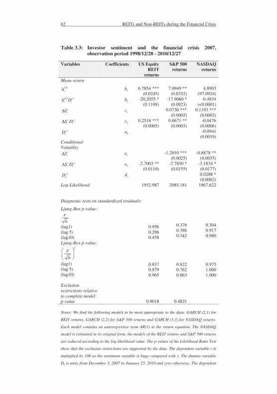
62 REITs and Non-REITs during the Financial Crisis
Table 3.3: Investor sentiment and the financial crisis 2007, observation period 1998/12/28 - 2010/12/27
Variables Coefficients US Equity REIT
returns
S&P 500 returns
NASDAQ returns
Mean return
0.5th 1b 6.7854 ***
(0.0245) 7.0949 **
(0.0332) 4.8903
(97.0924) 0.5 crt th D 2b -20.2055 *
(0.1199) -17.9060 *
(0.0923) -0.4834
(<0.0001) rtSΔ 1c 0.0730 ***
(0.0002) 0.1193 ***
(0.0002) r crt tS DΔ 2c 0.2518 ***
(0.0005) 0.0671 **
(0.0003) -0.0476
(0.0006) crtD 2a -0.0941
(0.0019) Conditional Volatility
vtSΔ 1e -1.2010 ***
(0.0025) -0.8878 **
(0.0035) v cvt tS DΔ 2e -2.7003 **
(0.0110) -2.7850 * (0.0155)
-3.1834 * (0.0177)
cvtD 2d 0.0288 *
(0.0002) Log-Likelihood 1952.987 2085.181 1867.622
Diagnostic tests on standardized residuals:
Ljung-Box p-value:
h
ε
(lag1) (lag 5) (lag10)
0.956 0.296 0.458
0.376 0.386 0.342
0.304 0.917 0.980
Ljung-Box p-value: 2
h
ε
(lag1) (lag 5) (lag10)
0.837 0.879 0.965
0.822 0.762 0.863
0.975 1.000 1.000
Exclusion restrictions relative to complete model: p-value
0.9018 0.4821
Notes: We find the following models to be most appropriate to the data: GARCH (2,1) for
REIT returns, GARCH (2,2) for S&P 500 returns and GARCH (3,3) for NASDAQ returns.
Each model contains an autoregressive term AR(1) in the return equation. The NASDAQ
model is estimated in its original form, the models of the REIT returns and S&P 500 returns
are reduced according to the log-likelihood value. The p-values of the Likelihood Ratio Test
show that the exclusion restrictions are supported by the data. The dependent variable r is
multiplied by 100 as the sentiment variable is huge compared with r. The dummy variable
Dt is unity from December 3, 2007 to January 25, 2010 and zero otherwise. The dependent

REITs and Non-REITs during the Financial Crisis 63
variables are the returns of REITs, S&P 500 and NASDAQ. The Ljung-Box Q-statistics tests
for serial correlation in standardized residuals and squared standardized residuals for lags
up to 27. Parameter estimates and standard errors (in parentheses) are listed. * Indicates
significance at the 10% level, ** indicates significance at the 5% level, *** indicates
significance at the 1% level.
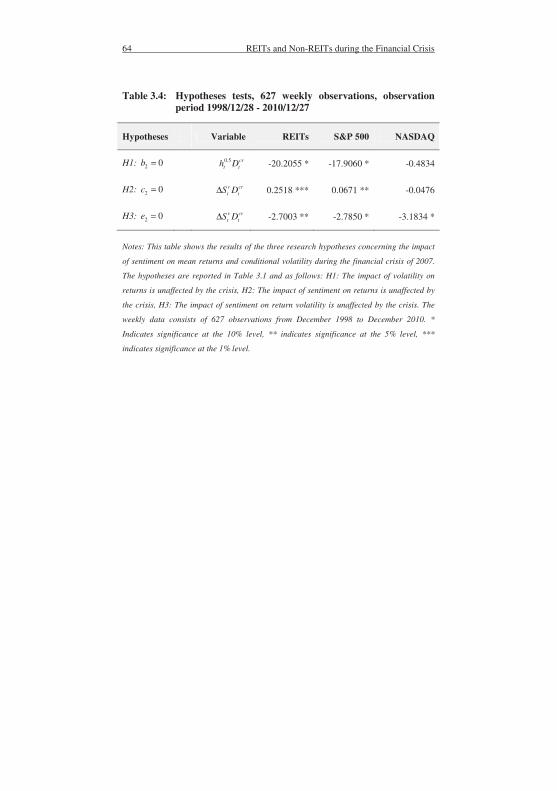
64 REITs and Non-REITs during the Financial Crisis
Table 3.4: Hypotheses tests, 627 weekly observations, observation period 1998/12/28 - 2010/12/27
Hypotheses Variable REITs S&P 500 NASDAQ
H1: 2 0b = 0.5 crt th D -20.2055 * -17.9060 * -0.4834
H2: 2 0c = r crt tS DΔ 0.2518 *** 0.0671 ** -0.0476
H3: 2 0e = v cvt tS DΔ -2.7003 ** -2.7850 * -3.1834 *
Notes: This table shows the results of the three research hypotheses concerning the impact
of sentiment on mean returns and conditional volatility during the financial crisis of 2007.
The hypotheses are reported in Table 3.1 and as follows: H1: The impact of volatility on
returns is unaffected by the crisis, H2: The impact of sentiment on returns is unaffected by
the crisis, H3: The impact of sentiment on return volatility is unaffected by the crisis. The
weekly data consists of 627 observations from December 1998 to December 2010. *
Indicates significance at the 10% level, ** indicates significance at the 5% level, ***
indicates significance at the 1% level.
Impact of Consumer Sentiment on New Home Sales 65
4 The Impact of Consumer Sentiment
on the Number of New Home Sales
Co-author of this chapter is J. Zietz.
4.1 Introduction
In financial markets the assumption that investors act fully rationally
and build their decisions on all available information has often been
challenged by phenomena that appear to contradict this paradigm,
such as excessive volatility or mean reversion of stock prices. One
explanation for these phenomena are the actions of so called noise
traders (Black, 1986). Noise traders suffer from cognitive biases,
such as overconfidence or overreaction.18 They rely to some degree
on sentiment and disturb the market with their irrational trading.
Baker and Wurgler (2007) define investor sentiment as a prospect
about the development of future cash flows and investment risks
based on information that is not justified by fundamentals. This
misguided belief may be based, for example, on general market
commentaries.
18 These cognitive biases have been researched by psychologists such as Tversky and Kahneman (1974, 1981), DeBondt and Thaler (1985), Barberis et al. (1998).
A. Mathieu, Essays on the Impact of Sentiment on Real Estate Investments, Essays in Real Estate Research 9, DOI 10.1007/978-3-658-11637-8_4,© Springer Fachmedien Wiesbaden 2016

66 Impact of Consumer Sentiment on New Home Sales
Efficient market theory assumes that the mispricing caused by noise
traders is quickly eliminated by the countertrading of sophisticated
arbitrageurs.19 But the trading of noise traders is unpredictable as the
beliefs of noise traders are uncertain. According to Daniel et al.
(2001) arbitrageurs are risk-averse; in the short run, however, they
face the risk that sentiment becomes more extreme and prices
deviate further from their fundamental values. The so called
systematic “noise trader risk” (DeLong et al. 1990) and the accruing
transaction costs (Shleifer and Vishny, 1997) prevent sophisticated
arbitrageurs to fully offset the mispricing. Thus, noise trading has a
persistent impact on financial markets.
Real estate markets are substantially different from financial
markets. They are characterized by heterogeneity, illiquidity, high
transaction costs and a lack of information (Lin and Vandell, 2007).
Unlike for stocks, for properties no perfect substitute exists. This
makes a comparison of prices difficult. Further, a new home requires
a high capital commitment and is not easily resold quickly.
Information on fundamentals is asymmetric between the seller and
the buyer of the property. In contrast to the builder the buyer does
not exactly know the quality and basic structure of the building.
According to Palomino (1996), noise traders in financial markets
primarily invest in small stocks that tend to be less liquid and more
19 Fama (1965) developed the efficient market hypothesis, Samuelson (1965) published a proof of the hypothesis and Fama (1970) improved the theory.

Impact of Consumer Sentiment on New Home Sales 67
volatile than large stocks. Thus, if small imperfections, such as less
liquidity, can cause more activity of noise traders in financial
markets, real estate markets that are characterized by several
imperfections should be even more prone to the influence of
sentiment than financial markets.
Even though real estate markets and stock markets differ, the
investors in these markets are not necessarily different. In capital
markets, noise traders are often identified as individual investors
(Glushkov, 2006). They are more prone to cognitive biases and,
therefore, more sensitive to changes in sentiment. New one-family
homes are not in the focus of institutional investors, but they are
interesting for individuals. As individuals react irrationally in their
stock investment decisions, why should they behave differently in
their real estate investment decisions? The risk that triggers irrational
behavior is similar in both markets (illiquidity, high transaction
costs) and even more pronounced in direct real estate markets. Thus,
if individuals rely on investor sentiment in capital markets, they
probably rely on consumer sentiment in direct real estate markets.
In our study we investigate if consumer sentiment has an impact on
the decision of a household to buy a new home. If consumer
sentiment has an impact, one would expect that positive consumer
sentiment is attended by more sales of new one-family homes. In a
positive market environment, employment is more stable and
households feel more confident to take on a large investment, such
as a house. Negative consumer sentiment would indicate an unstable

68 Impact of Consumer Sentiment on New Home Sales
market environment and would probably prevent households from
investing directly in real estate.
The decision of a household to buy a new one-family house depends
on several factors. Some of these factors are not easy measurable or
no relevant data exist. As not all influencing factors are available and
we are primarily interested in one variable, the consumer sentiment,
we use an unobserved component model (UCM) that can deal with
omitted variables far better than least squares.
We find that two of our five tested macroeconomic variables have a
statistically significant impact on the number of new one-family
home sales in the U.S. from 1978 to 2010. The consumer sentiment
has a significantly positive impact and the mortgage rate a strongly
negative impact on the number of new home sales. Taken together
both variables explain approximately 23 percent of the variation in
the number of new one-family home sales. Our analysis shows that
apart from monetary aspects expectations also strongly influence
investment decisions of individuals.
The remainder of the study proceeds as follows. In the literature
review we discuss sentiment studies in the field of real estate and,
more generally, studies relating to potential cognitive biases of
individuals. The methodology section presents different unobserved
component models that are used for our analysis. The results section
contains our empirical findings and the concluding section
summarizes the main aspects of the study.

Impact of Consumer Sentiment on New Home Sales 69
4.2 Literature Review
Behavioral finance literature has developed several cognitive biases
in the beliefs of investors that allow sentiment to play a role in
financial markets. Daniel et al. (1998 and 2001) explain patterns in
stock returns using two cognitive biases in investors’ beliefs:
“overconfidence” and “self-attribution”. “Overconfidence” about
private information lets investors overreact and causes long-lag
autocorrelations or excessive volatility. “Self-attribution” bias
(attributing success to their own expertise and failures to external
factors) extends overreaction and implies short-term momentum as
well as long-term reversals.
Barberis and Huang (2001) analyze the “mental accounting”, which
describes the evaluation of individuals concerning financial
transactions. Accordingly, individuals assign their assets to discrete,
non-transferable groups and each group is related to a different level
of utility. Investors’ attitude towards risk is described by the
cognitive biases “loss aversion” and “narrow framing”. Kahneman
and Tversky (1979) develop in their prospect theory the idea of “loss
aversion”, meaning that individuals are more sensitive to losses than
to gains. “Narrow framing” indicates that individuals look after
narrowly defined gains and losses. Barberis and Huang (2001) find
evidence that the beliefs of investors in individual stocks as well as
in a stock portfolio are influenced by both cognitive biases: “loss

70 Impact of Consumer Sentiment on New Home Sales
aversion” and “narrow framing”. All these cognitive biases let some
financial investors become susceptible to the impact of investor
sentiment. Their irrational trading causes financial markets to
become inefficient.
The impact of investor sentiment on indirect real estate investments,
such as real estate investment trusts or stocks of property companies,
has been analyzed in few studies. Barkham and Ward (1999)
investigate the discount of property company shares to their net asset
value (NAV). They conclude that, in addition to agency costs,
contingent taxation, and the liquidity of assets, investor sentiment
explains a significant part of these discounts. Other studies analyze
the relationship between investor sentiment and REIT returns. Lin et
al. (2009) find a strong impact of investor sentiment on the return
generating process of REITs. Clayton and MacKinnon (2002)
identify a relationship between sentiment and the discount to net
asset value in REIT pricing.
There has been only little research on the impact of sentiment on
direct real estate investment. Gallimore and Gray (2002) design a
questionnaire survey and ask UK investment decision makers if
investor sentiment plays a role in their decision making. They find
strong support for investor sentiment as an important source of
information. Ling (2005) analyzes the ability of institutional
managers to predict commercial real estate return performance. One
result of the study is the evidence for cognitive biases in the beliefs
of commercial real estate investors. The behavioral finance literature

Impact of Consumer Sentiment on New Home Sales 71
describes the associated behavior as “representativeness bias”, which
means that recent returns are overweighted and long-term
performance is underweighted. Clayton et al. (2009) investigate the
impact of fundamentals and investor sentiment on commercial real
estate valuation using an error correction model. They find evidence
that investor sentiment has a significant impact on real estate pricing.
As financial investors are susceptible to cognitive biases, households
may also be. A new home investment decision is of course different
from the decision to sell or buy stocks. An investment in a new home
is long-term; it implies higher capital spending and a resale is more
difficult given the illiquidity of the real estate market. But “loss
aversion” and “narrow framing” may also affect the beliefs of
individuals and, hence, influence their investment decision for direct
real estate investments. If households suffer from the same cognitive
biases as financial investors, consumer sentiment is bound to have an
impact on their decision process.
4.3 Data
We use monthly data from August 1978 to August 2010 on the
number of new home sales in the U.S., the consumer sentiment, the
mortgage rate, the inflation rate, real estate loans and the disposable
personal income. All data are from the Federal Reserve Bank of St.

72 Impact of Consumer Sentiment on New Home Sales
Louis data bank. The variables consist of 385 observations. Table 4.1
provides variable names and their definitions.
The Bureau of the Census publishes every month data on “new home
sales”, which reports sales of newly constructed one-family homes in
the U.S. This variable seems to be appropriate for our analysis
because it relates to transactions, unlike variables, such as building
permits or housing starts, which are only declarations of intent. The
data are reported at seasonally adjusted annual rates. Hamilton
(2008) also uses this variable to identify the impact of monetary
policy on new home sales.
To capture sentiment, we use a consumer sentiment index instead of
an investor sentiment index because it is primarily individuals and
not institutional investors who buy new one-family houses. We
employ the University of Michigan Consumer Sentiment Index
published monthly by the University of Michigan and Thomson
Reuters Datastream. The base year of the index (a value of 100) is
1966. Each month, the University of Michigan’s survey research
center interviews a random sample of approximately 500 U.S.
households. 50 core questions are asked with focus on the prospects
of the personal financial situation, the short-term general economy
and the long-term economic outlook. The data are not seasonally
adjusted. The consumer sentiment variable is a common variable in
studies that try to explain the relationship between movements in
consumer sentiment and the economic development (for example,
Souleles, 2004, Otoo, 1999).

Impact of Consumer Sentiment on New Home Sales 73
The mortgage rate is the 30-year conventional mortgage rate in
percentage format. It has a direct impact on the costs that accrue with
the purchase of a new home. The lower the mortgage rate is the
lower are the corresponding costs. Dua and Smyth (1995) analyze
the usefulness of the mortgage rate amongst other macroeconomic
variables to predict sales of homes.
The real estate loans variable is seasonally adjusted and based on
information from all commercial banks in the U.S. Real estate loans
are loans secured by real estate. Thus, we expect a positive
relationship between real estate loans and new home sales.
The University of Michigan inflation expectation is part of the
survey for the consumer sentiment index. Since 1977, the U.S.
households have been asked about their expectation concerning the
rise in prices over the next year and the next five to ten years. Bond
and Seiler (1998) find that residential real estate is a significant
hedge against expected and unexpected inflation. Thus, we expect a
positive relationship between the number of new home sales and the
inflation rate.
Disposable income is the difference between total personal income
and personal current taxes; the data are reported at seasonally
adjusted annual rates. Dua et al. (1999) also use this variable to
analyze the usefulness of different leading indicators in predicting
U.S. home sales. As a higher disposable income enables more

74 Impact of Consumer Sentiment on New Home Sales
individuals to buy a new home, we expect a positive relationship
between both variables.
Figure 4.1 shows time-plots of each data series. The new home sales
rate has its peak in 2005 and then declines until the end of 2008 from
approximately 1400 to 150; it shows five to ten year cyclical
behavior. The time series of the mortgage rate and the inflation rate
are similar with peaks in 1981 and 1980, when the U.S. were in a
deep recession. Consumer sentiment shows ten year cyclical
behavior and has its low in 1980 and in 2008, both times preceding a
recession. Real estate loans and disposable personal income behave
similarly and rise continuously.
4.4 Methodology
For our analysis we rely on an UC model instead of an OLS
regression. The key advantage of the UCM in our particular
application is the fact that it is possible to reliably identify the
coefficients of some observable determinants of the dependent
variable even if some independent variables are omitted. These other
independent variable may be known to play a role in determining the
dependent variable, but may be impossible to measure; alternatively,
and more to the point for the current application, there may not be a
reliable or generally accepted theory to suggest which these other
variables are. In any case, the influence of these omitted independent
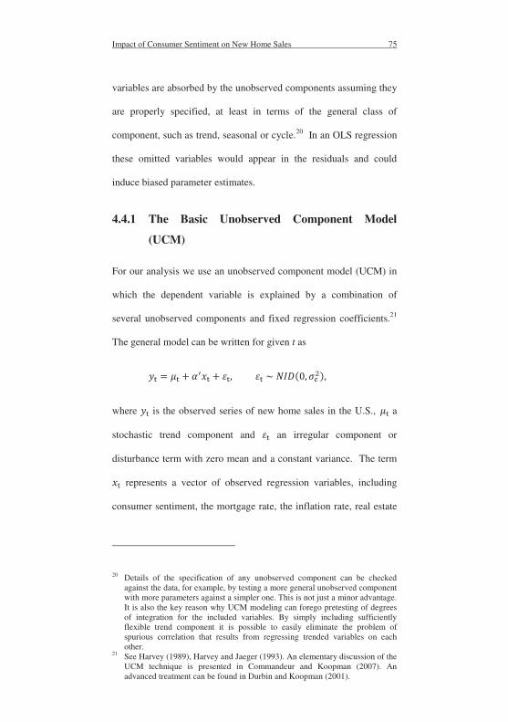
Impact of Consumer Sentiment on New Home Sales 75
variables are absorbed by the unobserved components assuming they
are properly specified, at least in terms of the general class of
component, such as trend, seasonal or cycle.20 In an OLS regression
these omitted variables would appear in the residuals and could
induce biased parameter estimates.
4.4.1 The Basic Unobserved Component Model
(UCM)
For our analysis we use an unobserved component model (UCM) in
which the dependent variable is explained by a combination of
several unobserved components and fixed regression coefficients.21
The general model can be written for given t as
where is the observed series of new home sales in the U.S., a
stochastic trend component and an irregular component or
disturbance term with zero mean and a constant variance. The term
represents a vector of observed regression variables, including
consumer sentiment, the mortgage rate, the inflation rate, real estate
20 Details of the specification of any unobserved component can be checked against the data, for example, by testing a more general unobserved component with more parameters against a simpler one. This is not just a minor advantage. It is also the key reason why UCM modeling can forego pretesting of degrees of integration for the included variables. By simply including sufficiently flexible trend component it is possible to easily eliminate the problem of spurious correlation that results from regressing trended variables on each other.
21 See Harvey (1989), Harvey and Jaeger (1993). An elementary discussion of the UCM technique is presented in Commandeur and Koopman (2007). An advanced treatment can be found in Durbin and Koopman (2001).

76 Impact of Consumer Sentiment on New Home Sales
loans and disposable personal income; is an appropriately
dimensioned vector of regression coefficients.
In the so-called local linear trend model the term is modeled as a
random walk with a stochastic drift term ,
(2)
(3)
where the level disturbance ( ), and the slope disturbance ( are
assumed uncorrelated with each other and also with the irregular
term ( ). The stochastic drift term also follows a random walk.
The trend component is fully determined by the variances
and , which are the only estimable parameters in the trend
Equations (2) and (3). In all of our models we set equal to zero;
this is similar to the approach taken by the Hodrick-Prescott filter
and generates a smooth trend model with a fixed level and a
stochastic drift. The only estimable parameter left for the stochastic
trend is .
4.4.2 A Model with Additional Components
In models where significant autocorrelation arises in the irregular
component, we supplement the trend component with a first-order
autoregressive component. The AR(1) component captures the fact
that the number of new home sales tends to be persistent over time.
For given observation t, Equation (1) then takes the form

Impact of Consumer Sentiment on New Home Sales 77
where the AR term can be written as
The AR(1) coefficient is restricted to be less than unity to represent
a stationary process. This is necessary to avoid a situation where the
AR(1) coefficient is confounded with the random walk component in
the stochastic trend.22 Instead of an AR(1) component we also try a
stochastic cycle component ( in some of our models. This
alternative unobserved component can be incorporated for given t as
follows:
with
(
where the stochastic cycle component is constructed as a sine-
cosine wave with the disturbances and and a damping factor ,
which satisfies . is the frequency (in radians) with
. If becomes zero or , the stochastic cycle becomes
an AR(1) process. The two disturbances and are white noise
and assumed mutually uncorrelated with zero means and common
22 See Koopman et al. (2009) STAMP 8.2

78 Impact of Consumer Sentiment on New Home Sales
variance . The period in months is . Stochastic cycles of
this type are appropriate to model the “pseudo-cyclical behavior” of
many time series (Koopman et al., 2009).

Impact of Consumer Sentiment on New Home Sales 79
4.5 Empirical Results
In this section we present the empirical evidence on the impact of
consumer sentiment and other explanatory variables on the number
of sales of new one-family homes in the U.S. In our analysis we test
four different models. Model I and Model II differ in the number of
the regression coefficients. In Model I we include all of our five
variables. In Model II and in Models III and IV we remove the
variables with insignificant coefficients and only analyze the impact
of consumer sentiment and the mortgage rate on the number of new
one-family home sales. Model III is similar to Model II, but the
AR(1) component is omitted. In Model IV we include a stochastic
cycle component.
4.5.1 Summary Statistics
Table 4.2lists the summary statistics for all variables. All variables
except for the inflation rate have a kurtosis smaller than three and,
therefore, display a platykurtic pattern; the inflation rate, however, is
leptokurtic, distributed with a kurtosis of approximately 3.97. The
consumer sentiment is the only negatively skewed variable; the other
variables are positively skewed. A negative skew means that the
distribution has relatively few low values. In Figure 4.2 we see that
the left tail of the density distribution of the consumer sentiment is
longer compared with the density distribution of the mortgage rate
or the new home sales. The distribution of the consumer sentiment

80 Impact of Consumer Sentiment on New Home Sales
is left-skewed. The other variables are right-skewed and have
relatively few high values but many low values.
4.5.2 UCM with all Variables
Model I in Table 4.3 includes a trend component, a first-order
autoregressive component, and a regression component with five
variables. The variables consumer sentiment and disposable personal
income have a positive sign whereas the mortgage rate, real estate
loans and inflation rate are negatively related to the number of new
home sales. The consumer sentiment and the mortgage rate are the
only variables with statistically significant coefficients; the three
other explanatory variables are insignificant and therefore excluded
from the further analysis. The statistical insignificance of the
inflation rate is interesting because several studies, for example
Hartzell et al. (1987) and Bond and Seiler (1998), identify real estate
investments as a good hedging instrument against anticipated and
unanticipated inflation. In Figure 4.1 we see that disposable personal
income and real estate loans increases continuously from 1978 until
2010 and the sales of new homes fluctuate relative intensely. This
can explain the result that no relation exists between the dependent
variable and the two explanatory variables. The Durbin Watson test
has a value of approximately two, which means that no
autocorrelation of the residuals exists. To compare the different
models we use R2 and Rd2 and the two information criteria Akaike
(AIC) and Bayesian (BIC). Rd2 compares the fit of the model with a

Impact of Consumer Sentiment on New Home Sales 81
random walk plus drift. It reveals how much of the variation in the
number of “new home sales” is explained by the regression variables
alone, whereas R2 measures how much is explained by the whole
right side of the equation, which includes all unobserved
components.

82 Impact of Consumer Sentiment on New Home Sales
4.5.3 UCM with Significant Variables
As three of the five explanatory variables are insignificant in Model
I, we include in Model II only the significant explanatory variables
consumer sentiment and the mortgage rate. The structure of the
model does not change, we have again a smooth trend model with a
fixed level and a stochastic drift, an AR(1) component and the
regression component. The variable consumer sentiment is now
significant at the five percent level; in Model I it is significant only
at the ten percent level. The mortgage rate is significant at the one
percent level in both models. To get an economic interpretation of
the estimated coefficients, we calculate elasticities at the mean for all
models and coefficients. The elasticities are listed in Table 4.4. The
impact of the mortgage rate is higher compared to that of the
consumer sentiment. A one percent increase in the mortgage rate in
Model II will lower new home sales by approximately 0.64 percent.
This result is intuitive as lower mortgage rates offer more people the
opportunity to buy a new home. The elasticity for consumer
sentiment of Model II is 0.13. A one percent increase in consumer
sentiment raises new home sales by approximately 0.13 percent. This
finding is in line with Weber and Devaney (1996), who ascertains
that consumer sentiment is useful to improve forecasts of housing
starts. Model II is the preferred model compared to Model I.
Although the coefficients of determination, Rd2 and R2, are larger in
Model I, the three additional included regression coefficients are

Impact of Consumer Sentiment on New Home Sales 83
insignificant. As a consequence, the information criteria AIC and
BIC are lower in Model II, which makes it the preferred model.

84 Impact of Consumer Sentiment on New Home Sales
4.5.4 Other Models
Model III provides a variation of Model II: the autoregressive
component is omitted. This lowers the Rd2 measure of fit compared
to Model II. As the two information criteria BIC and AIC are larger
in Model III compared to Models I and II, Model III is the inferior
model. Also, the Durbin Watson test has a value of approximately
1.5, which implies some residual autocorrelation.
Model IV modifies Model II by replacing the autoregressive
component with a stochastic cycle component. The stochastic cycle
component is specified in Equations (6)-(8). A cycle of the length of
twenty years appears appropriate for the data.23 In terms of the
coefficients of determination, Rd2 and R2, there is little change
relative to Model II. The same applies to the information criteria
AIC and BIC. As the coefficients of Model IV are also very close to
those of Model II, there is little point going from a simpler model,
with an autoregressive component, to a more complicated one, with
a cycle component.24 Thus, Model II remains the preferred model.
In Figure 4.3 we show for each model how much of the variation of
new home sales is explained by: (1) the stochastic trend, (2) the
stochastic trend plus the regression component, (3) the stochastic
23 We also try models with a cycle of five and ten years as well as multiple cycles; all of these models suffer from only weak convergence. As the time series of “new home sales” shows relatively irregular cycles, only a large cycle seems to be able to capture all the different structures.
24 We also test a model where we include both components, the autoregressive and the cycle component. But that does not change the results either.

Impact of Consumer Sentiment on New Home Sales 85
trend plus the autoregressive or cycle components and (4) by the
regression component alone. It is apparent that the regression
component alone can explain closely the downturn in new home
sales in the early 1980s and the subsequent upturn in the middle of
the 1980s. It can also capture the ups and downs during the 1990s.
However, the regression component (consumer sentiment and
mortgage rate) fails to predict the downturn around 1990 and, in
particular, the crisis around 2008. That means that the two recent
downturns (1990 and 2008) in new home sales are not predictable by
sentiment or the mortgage rate. There are other forces at work. These
are captured by our stochastic trend component. As a result, the trend
and the regression component taken together well approximate the
behavior of new home sales over time, either one alone does not.
Figure 4.4 provides some graphical evidence on the residual fit of
Models I through IV. The autocorrelation functions (ACF’s) show
no autocorrelation of the residuals of Model I, II and IV. In Model
III however the ACF’s display some autocorrelation of the residuals
at lags one and four. The QQ normality plots of Model II and IV
reveal that the residuals are nearly normally distributed. The Cusum
plot identifies no sign of a structural change as the upper and lower
limits are not crossed.
In summary, Model II is appropriate to explain the variation of the
number of new one-family home sales in the U.S. The variables
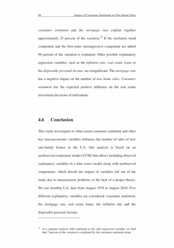
86 Impact of Consumer Sentiment on New Home Sales
consumer sentiment and the mortgage rate explain together
approximately 23 percent of the variation.25 If the stochastic trend
component and the first-order autoregressive component are added
96 percent of the variation is explained. Other possible explanatory
regression variables, such as the inflation rate, real estate loans or
the disposable personal income, are insignificant. The mortgage rate
has a negative impact on the number of new home sales. Consumer
sentiment has the expected positive influence on the real estate
investment decisions of individuals.
4.6 Conclusion
This study investigates to what extent consumer sentiment and other
key macroeconomic variables influence the number of sales of new
one-family homes in the U.S. Our analysis is based on an
unobserved component model (UCM) that allows including observed
explanatory variables in a time series model along with unobserved
components, which absorb the impact of variables left out of the
study due to measurement problems or the lack of a proper theory.
We use monthly U.S. data from August 1978 to August 2010. Five
different explanatory variables are considered: consumer sentiment,
the mortgage rate, real estate loans, the inflation rate and the
disposable personal income.
25 In a separate analysis with sentiment as the only regression variable, we find that 7 percent of the variation is explained by the consumer sentiment alone.

Impact of Consumer Sentiment on New Home Sales 87
We analyze UCMs with various structures: the models differ in the
number of explanatory variables and the inclusion of different
unobserved components. A smooth trend model together with an
AR(1) component and the two observed regression variables
consumer sentiment and mortgage rate appear to be most
appropriate for the data. The other explanatory regression variables
are insignificant. That includes the inflation rate, which is somewhat
surprising as it is often thought that inflation motivates individuals to
invest in real estate.
The results of our analysis indicate that consumer sentiment has a
significantly positive impact on the number of new one-family home
sales in the U.S. An increase in the consumer sentiment index
suggests that people expect a positive development of their personal
financial situation, both in the short-term and the long-term. These
prospects positively influence their investment decision concerning a
new home. A decrease in the consumer sentiment index, however,
suggests negative prospects and leads to a reduction in the number of
new home sales.
The mortgage rate is also significant and has the expected strongly
negative impact on the number of new home sales. Lower mortgage
rates offer the opportunity to buy a new home at lower costs. In
contrast to the consumer sentiment, the mortgage rate has a directly
calculable impact on the number of new home sales. The impact of
consumer sentiment on the investment decisions of individuals is
indirect and expressed in the expectations of individuals. Both

88 Impact of Consumer Sentiment on New Home Sales
variables taken together explain approximately 23 percent of the
variation in the number of new one-family home sales.
We further determine that the regression component (consumer
sentiment and mortgage rate) taken together with the stochastic trend
component well approximate the behavior of new home sales over
time. The regression component alone however captures only partly
the variation in new home sales. In particular it fails to predict the
crisis around 2008.
In summary, our study is the first to investigate the relation between
residential real estate and consumer sentiment. We add to the
understanding of private investment decisions and show that the
impact of sentiment is not a topic exclusively of interest for financial
markets. The results of the study show that the imperfections of
direct real estate markets, such as heterogeneity, illiquidity, high
transaction costs and insufficient information, induce risk and make
real estate markets susceptible to the impact of sentiment.

Impact of Consumer Sentiment on New Home Sales 89
4.7 Appendix for Chapter Four
Table 4.1: Variable Definitions, 385 monthly observations, observation period 1978/08 - 2010/08
Variables Variable Definition
New home sales New one-family homes sold: United States, in thousands,
seasonally adjusted annual rate (SAAR)
Consumer
sentiment
University of Michigan: Consumer Sentiment Index, first
quarter 1966 = 100, not seasonally adjusted (NSA)
Mortgage rate 30- year conventional mortgage rate, in percent
Real estate loans Real estate loans at all commercial banks, billions of
dollars, seasonally adjusted (SA)
Inflation rate University of Michigan inflation expectation, in percent
Disposable
personal income
Disposable personal income: per capita: current dollars,
seasonally adjusted annual rate (SAAR)
Notes: All data are collected from the Federal Reserve Bank of St. Louis.

90 Impact of Consumer Sentiment on New Home Sales
Table 4.2: Summary Statistics, 385 monthly observations, observation period 1978/08 - 2010/08
Variables Mean Standard Deviation
Minimum Maximum Skewness Kurtosis
New home sales
681.1500 211.4300 282.0000 1389.0000 0.8418 0.6234
Consumer sentiment
86.2790 13.0640 51.7000 112.0000 -0.4493 -0.5264
Mortgage rate
8.9370 2.8430 4.4300 18.4500 1.0997 0.9245
Real estate loans
877.6800 1071.9000 24.9000 3877.7000 1.4768 1.1403
Inflation rate
3.7490 1.8490 0.4000 10.4000 2.1653 3.9687
Disposable personal income
14407.0000 10883.0000 1938.0000 37419.0000 0.5416 -0.9723
Notes: All data relate to the U.S. for the time period of August 1978 to August 2010. We
have 385 monthly observations.

Impact of Consumer Sentiment on New Home Sales 91
Table 4.3: Results of the UCMs, 385 monthly observations, observation period 1978/08 - 2010/08
Variables Model I Model II Model III Model IV
Consumer sentiment 0.9526 *
(0.5300)
1.0257 **
(0.5202)
1.0792 **
(0.4747)
1.0286 **
(0.5203)
Mortgage rate -49.4396 ***
(5.3679)
-48.8059 ***
(5.2038)
-50.6575 ***
(4.6202)
-48.7972 ***
(5.2047)
Real estate loans -0.1200
(0.1204)
Inflation rate -1.2902
(5.3044)
Disposable personal income
0.0147
(0.0131)
Rd2 0.2399 0.2291 0.1710 0.2292
R2 0.9621 0.9616 0.9587 0.9616
AIC 7.6518 7.6423 7.7151 7.6422
BIC 7.7339 7.6936 7.7665 7.6936
Durbin-Watson 2.0015 1.9961 1.5450 2.0034
Notes: All models contain a smooth stochastic trend – a combination of a fixed level and a
stochastic slope. All data relate to the U.S. for the time period of August 1978 to August
2010. We have 385 monthly observations. The dependent variable is the number of new
one-family home sales in the U.S. Each model shows strong convergence. Model I-IV are
unobserved component models. Parameter estimates and root mean squared errors (in
parentheses) are listed. * Indicates significance at the 10% level, ** indicates significance
at the 5% level, *** indicates significance at the 1% level.
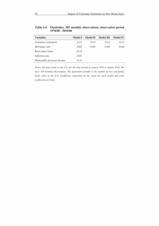
92 Impact of Consumer Sentiment on New Home Sales
Table 4.4: Elasticities, 385 monthly observations, observation period 1978/08 - 2010/08
Variables Model I Model II Model III Model IV
Consumer sentiment 0.12 0.13 0.14 0.13
Mortgage rate -0.65 -0.64 -0.66 -0.64
Real estate loans -0.15
Inflation rate -0.01
Disposable personal income 0.31
Notes: All data relate to the U.S. for the time period of August 1978 to August 2010. We
have 385 monthly observations. The dependent variable is the number of new one-family
home sales in the U.S. Coefficient elasticities at the mean for each model and each
coefficient are listed.

Impact of Consumer Sentiment on New Home Sales 93
Figure 4.1: Dependent and explanatory variables over time
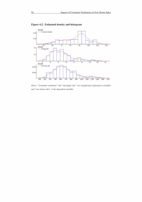
94 Impact of Consumer Sentiment on New Home Sales
Figure 4.2: Estimated density and histogram
Notes: “Consumer sentiment” and “mortgage rate” are (significant) explanatory variables
and “new home sales” is the dependent variable.

Impact of Consumer Sentiment on New Home Sales 95
Figure 4.3: Graphics of the different model results (Model I-IV)
Model I: contains a smooth stochastic trend, five explanatory
regression variables and an AR(1) component
Model II: contains a smooth stochastic trend, two explanatory
regression variables and an AR(1) component

96 Impact of Consumer Sentiment on New Home Sales
Model III: contains a smooth stochastic trend, two explanatory
regression variables and no AR(1) component
Model IV: contains a smooth stochastic trend, two explanatory
regression variables and a cycle component (20 years)

Impact of Consumer Sentiment on New Home Sales 97
Figure 4.4: Residual graphics of the different models (Model I-IV)
Model I: contains a smooth stochastic trend, five explanatory
regression variables and an AR(1) component
Model II: contains a smooth stochastic trend, two explanatory
regression variables and an AR(1) component
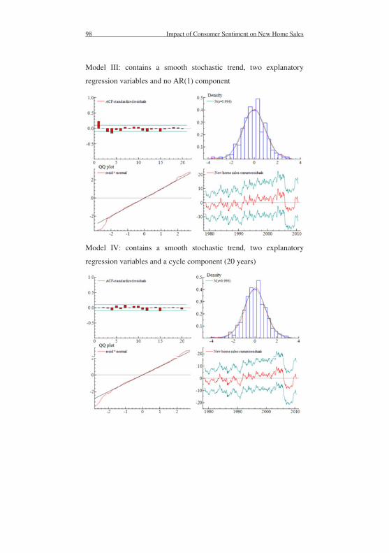
98 Impact of Consumer Sentiment on New Home Sales
Model III: contains a smooth stochastic trend, two explanatory
regression variables and no AR(1) component
Model IV: contains a smooth stochastic trend, two explanatory
regression variables and a cycle component (20 years)
Conclusions 99
5 Dissertation Conclusions
This dissertation is composed of three papers that examine the
impact of sentiment on direct and indirect real estate investments.
Papers one (Chapter two) and two (Chapter three) analyze the impact
of investor sentiment on real estate investment trusts (REITs) and
Paper three (Chapter four) investigates the relationship between
direct real estate investments and consumer sentiment.
In Paper one we analyze, on weekly data for the time period
December 1998 to May 2009, the influence of investor sentiment on
the returns and return volatilities of U.S. Equity REITS. We use two
different weekly sentiment indicators, one for individual investor
sentiment and one for institutional investor sentiment. Our main
findings suggest that individual investor sentiment is a significant
factor in explaining REIT returns and REIT return volatilities. We
can also identify asymmetric sentiment threshold values for both the
return and the conditional volatility parts of the model. Bad news
tends to have a more significant effect on the conditional volatility of
REITs than good news. In other words, bearish sentiment increases
REIT return volatility more than bullish sentiment does. This is
consistent with Barberis and Huangs’ (2001) finding that investors
are loss averse and focus on narrowly defined gains and losses.
A. Mathieu, Essays on the Impact of Sentiment on Real Estate Investments, Essays in Real Estate Research 9, DOI 10.1007/978-3-658-11637-8_5,© Springer Fachmedien Wiesbaden 2016

100 Conclusions
In terms of the mean return equation, we find that REIT returns
increase in bullish sentiment stages, whereas bearish sentiment has
no impact on REIT returns. This result is surprising as we expect a
decrease in REIT returns in bearish sentiment stages.
The results suggest that even small changes in sentiment have a
significant impact on the conditional volatility of REITs, as indicated
by relatively small corresponding threshold values. The threshold
values of the mean equation, however, are higher, which indicates
that not every small change in sentiment has an impact on REIT
returns.
In Paper two we investigate the differential impact of investor
sentiment on the formation of returns and conditional return
volatility of a REIT index as opposed to non-REIT market indices.
In contrast to prior empirical studies, we test this differential impact
as a function of the market environment and compare an ordinary
market situation to the financial crisis that started in 2007. We use a
weekly sentiment indicator for institutional investor sentiment and
study its impact on US Equity REIT returns, S&P 500 returns and
NASDAQ returns over the period from December 1998 to December
2010.
The results of our analysis indicate that investor sentiment has a
significant impact on the returns of all three asset classes. In ordinary
market situations, our different asset classes behave in a similar
manner. This result is inconsistent with Lee et al. (2002) who find
Conclusions 101
that sentiment has the most profound impact on small cap stocks,
which are primarily listed in the NASDAQ index.
During the financial crisis, the influence of investor sentiment on
REIT and S&P 500 returns is significantly stronger. NASDAQ
returns, however, are only affected by sentiment in tranquil markets,
indicating that these stocks are less influenced by extreme market
sentiment.
The correlation between the returns and changes in sentiment is
positive in both market situations. That means that noise traders’
optimism increases their demand and provides a higher risk
premium, which results in a higher return. However, if noise traders
are pessimistic they decrease their demand, lower the risk premium
and reduce the return.
We also find that REIT and S&P 500 returns are negatively
influenced by contemporaneous conditional volatility during the
financial crisis. This indicates that if noise traders’ misperceptions
are more severe and conditional volatility increases, then returns
decrease.
With regard to the conditional return volatility, we find a significant
and negative impact of investor sentiment for all three indices.
Bullish changes in sentiment result in a decrease of return volatility,
whereas bearish changes in sentiment lead to an increase of return
volatility. Again, the impact is significantly higher during the crisis.

102 Conclusions
Our analysis shows that REIT returns and conditional REIT return
volatility are significantly influenced by investor sentiment
especially in extreme sentiment stages. Therefore, although REITs
are subject to a specific regulatory and tax framework and offer
significant diversification benefits compared to other asset classes,
they should be treated similar to stocks. Shareholders and the
management of REITs should consider the development of investor
sentiment to better anticipate the return and conditional volatility of
REITs.
In Paper three we investigate to what extent consumer sentiment and
other key macroeconomic variables influence the number of sales of
new one-family homes in the U.S. Our analysis is based on an
unobserved component model (UCM) that allows omitting the
influence of variables that are difficult to obtain due to measurement
problems or the lack of a proper theory. We use monthly U.S. data
from August 1978 to August 2010. Five different explanatory
variables are considered: consumer sentiment, the mortgage rate, real
estate loans, the inflation rate and the disposable personal income.
The results of our analysis indicate that only two of our five
explanatory variables are significant: consumer sentiment and the
mortgage rate. Consumer sentiment has a significantly positive
impact on the number of new one-family home sales in the U.S. An
increase in the consumer sentiment index suggests that people expect
a positive development of their personal financial situation, both in
the short-term and the long-term. These prospects positively

Conclusions 103
influence their investment decision concerning a new home.
Likewise, a decrease in the consumer sentiment index suggests
negative prospects and leads to a reduction in the number of new
home sales.
The mortgage rate is also significant and has the expected strongly
negative impact on the number of new home sales. Lower mortgage
rates offer the opportunity to buy a new home at lower costs. In
contrast to the consumer sentiment variable, the mortgage rate has a
directly calculable impact on the number of new home sales. The
impact of consumer sentiment on the investment decisions of
individuals is indirect and expressed in the expectations of
individuals. Both variables taken together explain approximately 23
percent of the variation in the number of new one-family home sales.
We further determine that the regression component (sentiment
variable and mortgage rate) taken together with the stochastic trend
component well approximate the behavior of new home sales over
time. The regression component alone, however, captures only part
of the variation in new home sales. In particular, it fails to predict the
crisis around 2008.
Paper three adds to the understanding of private investment decisions
in real estate markets and shows that the impact of sentiment is not a
topic exclusively of interest for financial markets. The results of the
study show that the imperfections of direct real estate markets, such
as heterogeneity, illiquidity, high transaction costs and insufficient

104 Conclusions
information, induce risk and make real estate markets susceptible to
the impact of sentiment. This knowledge enables building companies
to consider consumer sentiment as an influencing factor in their
demand forecasts. Further, it can help individuals to optimize their
investment date, although there are several other non-measurable
factors besides sentiment that have an impact on this decision.

References 105
References
Anderson, R., Clayton, J., MacKinnon, G., Sharma, R. (2005).
“REIT returns and pricing: the small cap value factor.”
Journal of Property Research 22(4): 267-286.
Backus, D. K., Gregory, A. (1993). “Theoretical relations between
risk premiums and conditional variances.” Journal of
Business and Economic Statistics 11(2): 177–185.
Baker, M., Wurgler, J. (2007). “Investor sentiment in the stock
market.” Journal of Economic Perspectives 21(2): 129-151.
Barberis, N., Huang, M. (2001). “Mental accounting, loss aversion,
and individual stock returns.” Journal of Finance 56(4):
1247-1292.
Barberis, N., Shleifer, A. and Vishny, R. (1998). “A model of
investor sentiment.” Journal of Financial Economics, 49(3):
307–43.
Barkham, R. J., Ward, C. W. R. (1999). “Investor sentiment and
noise traders: discount to net asset value in listed property
companies in the U.K.” Journal of Real Estate Research
18(2): 291-312.
A. Mathieu, Essays on the Impact of Sentiment on Real Estate Investments, Essays in Real Estate Research 9, DOI 10.1007/978-3-658-11637-8,© Springer Fachmedien Wiesbaden 2016

106 References
Below, S. D., Stansell, S. R., Coffin, M. (2000). ”The determinants
of REIT institutional ownership: tests of the CAPM.” Journal
of Real Estate Finance and Economics 21(3): 263-278.
Black, F. (1986). “Noise.” Journal of Finance 41(3): 529-543.
Bollerslev, T. (1986). “Generalized autoregressive conditional
heteroscedasticity.” Journal of Econometrics 31(3): 307-327.
Bond, M. T., Seiler, M. J. (1998). “Real estate returns and inflation:
an added variable approach.” Journal of Real Estate
Research 15(3): 327-338.
Brown, G. W. (1999). “Volatility, sentiment and noise traders.”
Financial Analysts Journal 55(2): 82-90.
Brown, G. W., Cliff, M. T. (2004). “Investor sentiment and the near-
term stock market.” Journal of Empirical Finance 11(1): 1-
27.
Brown, G. W., Cliff, M. T. (2005). “Investor sentiment and asset
valuation.” Journal of Business 78(2): 405-440.
Campbell, J. Y., Hentschel, L. (1992). “No news is good news: an
asymmetric model of changing volatility in stock returns.”
Journal of Financial Economics 31(3): 281-318.
Chen, N. F., Kan, R., Miller, M. H. (1993). “Are the discounts on
closed-end funds a sentiment index?” Journal of Finance
48(2), 795-800.
References 107
Chopra, N., Lee, C. M. C., Shleifer, A., Thaler, R. (1993). “Yes,
discounts on closed-end funds are a sentiment index.”
Journal of Finance 48(2): 801-808.
Chui, A. C. W., Titman, S., and Wei, K. C. J. (2003).”The cross
section of expected REIT returns.” Real Estate Economics,
31(3): 451-479.
Clayton, J. F., Ling, D. C., Naranjo, A. (2009). “Commercial real
estate valuation: fundamentals versus investor sentiment.”
Journal of Real Estate Finance and Economics 38(1): 5-37.
Clayton, J. F., MacKinnon, G. H., (2001). “Explaining the discount
to NAV in REIT pricing: noise or information?” RERI
Working Paper.
Clayton, J. F., MacKinnon, G. H. (2002). “Departures from NAV in
REIT pricing: the private real estate cycle, the value of
liquidity and investor sentiment.” RERI Working Paper.
Clayton, J. F., MacKinnon, G. H. (2003). “The relative importance
of stock, bond and real estate factors in explaining REIT
returns.” Journal of Real Estate Finance and Economics
27(1): 39-60.
Commandeur, J. J. F., Koopman, S. J. (2007). “An introduction to
state space time series analysis.” Oxford University Press,
Oxford and New York.
108 References
Cotter, J., Stevenson, S. (2006). “Multivariate modeling of daily
REIT volatility.” Journal of Real Estate Finance and
Economics 32(3): 305-325.
Daniel, K. D., Hirshleifer, D. and Subrahmanyam, A. (1998).
“Investor psychology and security market under- and
overreactions.” Journal of Finance 53(6): 1839–1886.
Daniel, K. D., Hirshleifer, D., Subrahmanyam, A. (2001).
“Overconfidence, arbitrage and equilibrium asset pricing.”
Journal of Finance 56(3): 921–965.
De Bondt, W. F. M., Thaler, R. H. (1985). “Does the stock market
overreact?” Journal of Finance 40(3): 557–558.
DeLong, J. B., Shleifer, A., Summers, L. H., Waldmann, R. J.
(1989). “The size and incidence of losses from noise trading.”
Journal of Finance 44(3): 681-96.
DeLong, J. B., Shleifer, A., Summers, L. H., Waldmann, R. J.
(1990). “Noise trader risk in financial markets.” Journal of
Political Economy 98(4): 703-738.
Devaney, M. (2001). “Time varying risk premia for real estate
investment trusts: a GARCH-M.” Quarterly Review of
Economics and Finance 41(3): 335-346.
Dua, P., Miller, S. M., Smyth, D. J. (1999). “Using leading
indicators to forecast U.S. home sales in a bayesian vector
References 109
autoregressive framework.” Journal of Real Estate Finance
and Economics 18(2): 191-205.
Dua, P., Smyth, D. J. (1995). “Forecasting us home sales using bvar
models and survey data on households' buying attitudes for
homes.” Journal of Forecasting 14(3): 217-227.
Dumas, B., Kurshev, A., Uppal, R. (2005). “What can rational
investors do about excessivevolatility and sentiment
fluctuations?” NBER Working Paper.
Durbin, J., Koopman, S. J. (2001). “Time series snalysis by state
space methods.” Oxford University Press, Oxford and New
York.
Engle, R. F. (1982). “Autoregressive conditional heteroscedasticity
with estimates of variance of United Kingdom inflation.”
Econometrica 50: 987-1008.
Engle, R. F., Lilien, D. M., Robins, R. P. (1987). “Estimating time
varying risk premia in the term structure: the ARCH-M
model.” Econometrica 55: 391-407.
Falzon, R. (2002). “Stock market rotations and REIT valuation.”
Prudential Real Estate Investors, October: 1-10.
Fama, E. (1965). “The behavior of stock market prices." Journal of
Business 38(1), 34-105.
110 References
Fama, E. (1970).“Efficient capital markets: a review of theory and
empirical work.”Journal of Finance 25(2): 383–417.
Friedman, M. (1953). “The case for flexible exchange rates.” Essays
in Positive Economics, Chicago: University of Chicago
Press.
Gentry, W. M., Jones, C. M., Mayer, C. J. (2004). “REIT reversion:
stock price adjustments to fundamental value.” Working
Paper, Columbia University.
Ghosh, C., Miles, M., Sirmans, C. F. (1996). “Are REITs stocks?”
Real Estate Finance, Fall: 46-53.
Glosten, L. R., Jagannathan, R., Runkle, D. A. (1993). ”On the
relation between the expected value and the volatility of the
nominal excess return on stocks.” Journal of Finance 48(5):
1779-1801.
Glushkov, D. (2006). “ Sentiment beta.” Working Paper, University
of Pennsylvania.
Hamilton, J. D. (2008).” Daily monetary policy shocks and new
home sales.” Journal of Monetary Economics 55 (7): 1171-
1190.
Hartzell, D., Hekman, J. S., Miles, M. E. (1987). “Real estate
returns and inflation.” Real Estate Economics 15(1): 617-637.
References 111
Harvey, A. C. (1989). “Forecasting, structural time series models
and the kalman filter.” Cambridge University Press,
Cambridge.
Harvey, A. C., Jaeger, A. (1993). “Detrending, stylized facts and the
business cycle.” Journal of Applied Econometrics 8(3): 231-
247.
Hirshleifer, D., Subrahmanyam, A., Titman, S. (2006). “Feedback
and the success of irrational investors.” Journal of Financial
Economics 81(2): 311-338.
Hughen, J. C., McDonald, C. G. (2005). “Who are the noise
traders?” Journal of Financial Research 28(2): 281-298.
Hung, S.-Y. K., Glascock, J. L. (2010). “Volatilities and momentum
returns in real estate investment trust.” Journal of Real Estate
Finance and Economics 41(2): 126-149.
Kahneman, D., Tversky, A. (1979). “Prospect theory: an analysis of
decision under risk.” Econometrica 47(2): 263-292.
Kelly, M. (1997). “Do noise traders influence stock prices?” Journal
of Money, Credit and Banking 29(3): 351-364.
Kirchler, M. (2009). “Underreaction to fundamental information and
asymmetry in mispricing between bullish and bearish
markets. An experimental study.” Journal of Economic
Dynamics and Control 33(2): 491-506.

112 References
Koopman, S. J., Harvey, A. C., Doornik, J. A., Shephard, N.(2009).
“Structural time series analyser, modeller and predictor
STAMP 8.2.” Timber Lake Consultants Press, London.
Kyle, A. S., (1985). “Continuous auctions and insider trading.”
Econometrica 53(6): 1315-1535.
Lease, R. C., Lewellen, W. G., Schlarbaum, G. G. (1974). “The
individual investor: attributes and attitudes.” Journal of
Finance 29(2): 413-433.
Lee, W. Y., Jiang, C. X., Indro, D. C. (2002). “Stock market
volatility, excess returns, and the role of investor sentiment.”
Journal of Banking and Finance 26(12): 2277-2299.
Lee, C., Shleifer, A., Thaler, R. (1991). “Investor sentiment and the
closed-end fund puzzle.” Journal of Finance 46(1): 75-109.
Lee, S., Stevenson, S. (2007). “The substitutability of REITs and
value stocks.” Applied Financial Economics 17(7): 541-557.
Lin, C. Y., Rahman, H., Yung, K. (2009). “Investor sentiment and
REIT returns.” Journal of Real Estate Finance and
Economics 39(4): 450-471.
Lin, Z., Vandell, K. D. (2007). “Illiquidity and pricing biases in the
real estate market.” Real Estate Economics 35(3): 291–330.
References 113
Ling, D. C. (2005). “A random walk down main street: can experts
predict returns on commercial real estate?“ Journal of Real
Estate Research 27(2): 137-154.
Merton, R. C. (1980). “On estimating the expected return on the
market: an exploratory investigation.” Journal of Financial
Economics 8(4): 323-361.
Neal, R., Wheatley, S. M. (1998). “Do measures of investor
sentiment predict returns?” Journal of Financial and
Quantitative Analysis 33(4): 523-547.
Nelson, D. B. (1991). “Conditional heteroskedasticity in asset
returns: a new approach.” Econometrica 59: 347-370.
Otoo, M. W. (1999). “Consumer sentiment and the stock market.”
FEDS Working Paper, No. 99-60.
Palomino, F. (1996). “Noise trading in small markets.” Journal of
Finance 51(4): 1537-1550.
Peterson, J. D., Hsieh, C. (1997). “Do common risk factors in the
returns on stocks and bonds explain returns on REITs?” Real
Estate Economics 25(2): 321-345.
Samuelson, P. (1965). “Proof that properly anticipated prices
fluctuate randomly.” Industrial Management Review 6(2):
41-49.
114 References
Shleifer, A., Summers, L. H. (1990). “The noise trader approach to
finance.” Journal of Economic Perspectives 4(2): 19-33.
Shleifer, A., Vishny, R. (1997). “The limits to arbitrage.” Journal of
Finance 52(1): 35–55.
Sias, R. W., Starks, L. T., Tinic, S. M. (2001). “Is noise trader risk
priced?” Journal of Financial Research 24: 311–329.
Simon, S., Ng, W. L. (2009). “The effect of the real estate downturn
on the link between REITs and the stock market.” Journal of
Real Estate Portfolio Management 15(3): 211-219.
Souleles, N. S. (2004). “Expectations, heterogeneous forecast errors,
and consumption: micro evidence from the Michigan
consumer sentiment surveys.” Journal of Money, Credit, and
Banking 36(1): 39-72.
Stevenson, S. (2002). “An examination of volatility spillovers in
REIT returns.” Journal of Real Estate Portfolio Management
8(3): 229-238.
Swaminathan, B. (1996). “Time-varying expected small firm returns
and closed-end fund discounts.” Review of Financial Studies
9(3): 845-887.
Tversky, A., Kahneman, D. (1981). “The framing of decisions and
the psychology of choice.” Science 211 (4481): 453–458.

References 115
Tversky, A., Kahneman, D. (1974). “Judgment under uncertainty:
heuristics and biases.” Science 185 (4157): 1124–1131.
Weber, W., Devaney, M. (1996). “Can consumer sentiment surveys
forecast housing starts?” Appraisal Journal 64(4): 343-50.
Weiss, K. (1989). “The post-offering price performance of closed-
end funds.” Financial Management 18(3): 57-67.
Zweig, M. E. (1973). “An investor expectations stock price
predictive model using closed-end fund premiums.” Journal
of Finance 28(1): 67-87.


