Essays on an emerging stock market: the case of nairobi ...

ESSAYS ON AN EMERGING STOCK MARKET: THE CASE OF NAIROBI STOCK EXCHANGE H

(Statistical Distribution of Returns, Market Seasonality and Reactionsto Dividend Announcements)

lloBlJOHN ALMADILQBERE SCHOOL OF ECONOMICS UNIVERSITY OF NAIROBI

A THESIS SUBMITTED IN PARTIAL FULFILLMENT OF THE REQUIREMENTS FOR THE DEGREE OF DOCTOR OF

PHILOSOPHY IN ECONOMICS OF THE UNIVERSITY OF NAIROBI

University of NAIROBI Library

0501606 8

OCTOBER 2009

UNIVERSITY OF NAIROBIlibrary

DECLARATION

This thesis is my original work and has not been presented for a degree in any university

Signature. ......Date.., .....

John Almadi Obere

This thesis has been submitted for examination with our approval as university

supervisors

Signature ............. .Da.e J > .lUh 0<Xl

Prof. Germano Mwabu School of Economics University of Nairobi

s't

Signature..... ................................. *.....

Prof. Francis Mwega School of Economics University of Nairobi

n

ACKNOWLEDGEMENTS

This work would not have been possible without the contribution of many individuals.

Special thanks go to my supervisors, Professors Germano Mwabu and Francis Mwega,

for their guidance, selflessness and advice. Indeed, if I had half of their dedication, this

work would have taken a very short time to complete. In the same vein, I owe gratitude to

the African Economic Research Consortium (AERC) for offering me a generous

scholarship without which this study would never have materialized. I am grateful to my

classmates and friends, Anne, Nahu, Mtui, Epaphra, Ngasamiaku, Naomi, Pauline, Sylvia

and Steve for all their help during the time we were together. They provided the light

moments when things were hard.

I must sincerely thank all members of the Obere family, for their prayers and material

support, including putting up with my absence over the duration of this study. My dad,

Obere-Janam, and my brother, Eliud, provided me with the learning model which I have

emulated.

I, however, remain responsible for all the errors and inaccuracies which may remain.

iii

ABBREVIATIONS

ARCH Autoregressive Conditional Heteroskedasticity

EGARCH Exponential Autoregressive Conditional Heteroskedasticity

EMH Efficient Market Hypothesis

GARCH Generalised Autoregressive Conditional HeteroskedasticityNSE Nairobi Stock Exchange

TGARCH Threshold Autoregressive Conditional Heteroskedasticity

VAR Vector Autoregression

TABLE OF CONTENTS

ACKNOWLEDGEMENTS............................ iii

ABBREVIATIONS.........................................................................................................iv

TABLE OF CONTENTS..................................................................................................v

Abstract.........................................................................................................xi

CHAPTER ONE

Background, Research Problem and Study Objectives

1.0 Introduction...................................................................................................................... ]

1.1 The stock exchange market.............................................................................................. 1

1.2 The Nairobi Stock Exchange...........................................................................................2

1.3 Efficient market hypothesis................r........... ............................................................... 4

1.4 Statement of the problem................................................................................................ 5

1.5 Objectives of the study................................................................................................... 8

1.6 Justification of the study...,............................................................................................. 8

1.7 Organization of the thesis.................................. ............................................................ 8

REFERENCES..................................................................................................................... 10

CHAPTER TWO

Ordinary Shares at the Nairobi Stock Exchange: Statistical Distribution

of Returns, Share Pricing and Market Volatility

2.0 Introduction...................................................................................................................... 12

2.1 Literature review.............................................................................................................. 12

2.2 Methodology............................................ 15

2.2.1 Linearity and volatility of returns............................................................................16

2.2.2 Test for non-linearity.............................................................................................. 17

2.2.3 Test for volatility.....................................................................................................18

2.3 Empirical Results.............................................................................................................22

2.3.1 Descriptive results.................................................................................................. 22

2.3.2 Linearity test results................................................................................................ 33

2.3.3 Volatility test results............................................................................................... 45

2.4 Conclusion....................................................................................................................... 52

REFERENCES........................................................................................... '........................ 53

CHAPTER THREE

Stock Market Seasonality: Evidence from NSE

3.0 Introduction...................................................................................................................... 61

3.1 Literature Review.............................................................................................................61

3.2 Methodology................................................... 63

3.2.1 The OLS model...................................................................................................... 64

3.2.2 GARCH models............................................................. 64

3.3 Data and empirical results............................................................................................... 65

3.3.1 Data........................................................... 65

3.3.2 Graphical representation of results......................................................................... 66

3.3.2a Day-of-the-week effects........................................................................................66

3.3.2b Month-of-the-year effects......................................................................... 70

3.3.2c Quarter-of-the-year effects....................................................................................74

3.3.3 Estimation results............................................................ 77

3.3.3a Day-of-the-week effects........................................................................................77

3.3.3b Month-of-the year effects......................................................................................79

3.3.3c Quarter-of-the-year effects....................................................................................81

3.4 Conclusion....................................................................................................................... 83

REFERENCES...................................................................................................................... 86

vi

CHAPTER FOUR

Ordinary Share Prices and Dividend Announcements

4.0 Introduction.....................................................................................................................95

4.1 Literature Review............................................................................................................96

4.2 Methodology.................................................................................................................... 98

4.2.1 Detecting impact of a market event........................................................................ 98

4.2.2 Normal returns................................................................................ 101

4.2.3 Abnormal returns.....................................................................................................103

4.2.4 Hypothesis to be tested........................................................................................... 104

4.2.5 An alternative model for computing abnormal returns........................................... 106

4.2.6 Sampling strategy....................................................................................................106

4.2.7 Empirical models.....................................................................................................107

4.2.8 Data.............................................. 107

4.3 Results.............................................................................................................................107

4.3.1 CAR results............................................................................................................. 107

4.3.2 Regression results.................................................................................................. 117

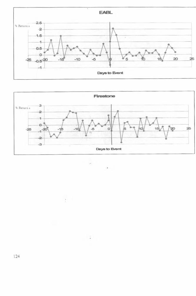
4.3.3 Graphical results........................... 122»

4.4 Conclusion.......................................................................................................................128

REFERENCES..................................................................................................................... 130

APPENDICES

APPENDIX 3.1 OLS results for day-of-the-week effect................................................... 88

APPENDIX 3.2 GARCH results for day-of-the-week effect............................ ................ 88

APPENDIX 3.3 TGARCH results for day-of-the-week effect..........................................89

APPENDIX 3 4 EGARCH results for day-of-the-week effect..........................................89

APPENDIX 3.5 OLS results for month-of-the-year effect................................................90

APPENDIX 3.6 GARCH results for month-of-the-year effect ........................................ 90

APPENDIX 3.7 TGARCH results for month-of-the-year effect....................................... 91

APPENDIX 3.8 TGARCH results for month-of-the-year effect....................................... 92

vii

APPENDIX 3.9 OLS results for quarter-of-the-year effect................................................92

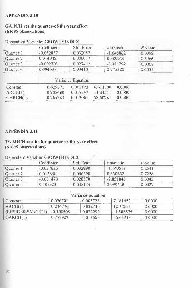
APPENDIX 3.10 GARCH results for quarter-of-the-year effects........................................93

APPENDIX 3.11 TGARCH results for quarter-of-the-year effects......................................93

APPENDIX 3.12 EGARCH results for quarter-of-the-year effects......................................94

LIST OF TABLES

Table 2.1 Trading characteristics of selected firms in NSE................................................. 21

Table 2.2 Descriptive group statistics for ordinary shares for selected firms in NSE...........32

Table 2.3 RESET results for selected firms in NSE.............................................................33

Table 2.4 GARCH (1, 1) results for selected firms in NSE.................................................. 45

Table 2.5 TGARCH results for selected firms in NSE .........................................................47

Table 2.6 EGARCH results for selected firms in NSE ........................................................ 49

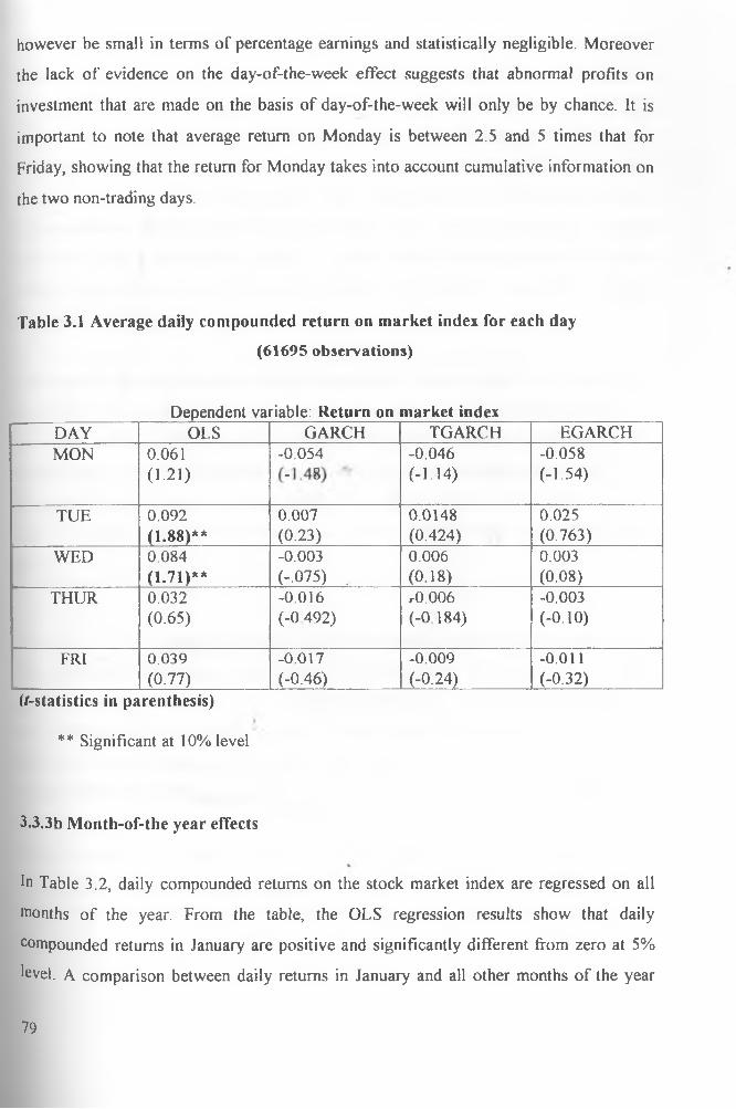
Table 3.1 Average daily compounded return on market index for each day........................ 78

Table 3.2 Average daily compounded return on market index for each month....................80

Table 3.3 Average daily compounded return on the overall market index ......................... 81

Table 4.1 CAR results...........................................................................................................108

Table 4.2 Cumulative abnormal returns.............................................................................. 116

Table 4.3Test for equality of medians between series......................................................... 116s’

Table 4.4Test for equality of variances between series.........................................................118

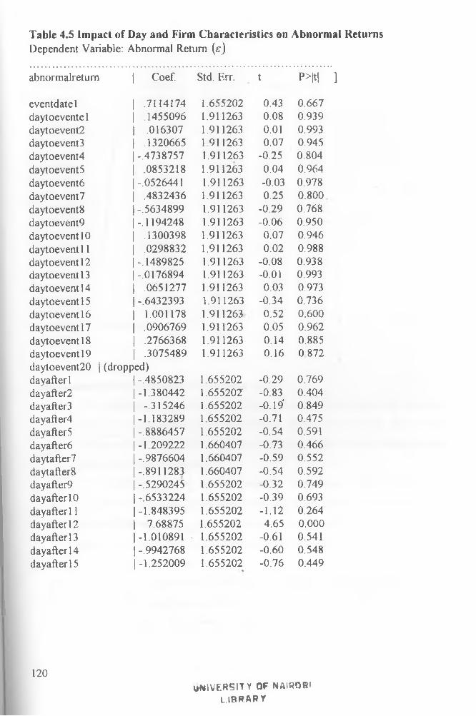
Table 4.5 Impact of Day and Firm Characteristics on Abnormal Returns..............................120

LIST OF FIGURES .

Figure 2.la Daily percentage change in ordinary share prices (Bamburi)............................ 23

Figure 2. lb Daily Percentage change in ordinary share prices (BOC)................................. 23

Figure 2. lc Daily percentage change in ordinary share prices (BAT)...................................24

Figure 2. Id Daily percentage change in ordinary share prices (Barclays)............................ 24

Figure 2.1e Daily percentage change in ordfnary share prices (DTB)...................................25

Figure 2. If Daily percentage change in ordinary share prices (Unilever)............................ 25

Figure 2. lg Daily percentage change in ordinary share prices (EABL)............................... 26

Figure 2.1 h Daily percentage change in ordinary share prices (G. Williamson)..................26

viii

Figure.2. li Daily percentage change in ordinary share prices (Kakuzi)............................. 27

Figure. 2.1 j Daily percentage change in ordinary share prices (KCB)................................. 27

Figure 2.1k Daily percentage change in ordinary share prices (Kenya Airways).................28

Figure.2.11 Daily percentage change in ordinary share prices (KPLC).............................. 28

Figure 2. lm Daily percentage change in ordinary share prices (NIC)................................. 29

Figure 2. In Daily percentage change in ordinary share prices (Nation)......................... 29

Figure 2.1o Daily percentage change in ordinary share prices (Sasini)..........................30

Figure 2.1 p Daily percentage change in ordinary share prices (Total Kenya).................... 30

Figure 2.1 q Daily percentage change in ordinary share prices (Firestone)......................... 31

Figure 2. lr Daily percentage change in ordinary share prices (TPS)..................................31

Figure 2.1s Daily percentage change in ordinary shares prices (STANCHART)................31

Figure 2.2a Recursive residual test (BAMBURI)..................................................................36

Figure 2.2b Recursive residual test (BOC)............................................................................ 36

Figure 2.2c Recursive residual test (BAT)............................................................................ 37

Figure 2.2d Recursive residual test (BARCLAYS)...................... 37

Figure 2.2e Recursive residual test (DTB)............................................................................ 38

Figure 2.2f Recursive residual test (UNILEVER)......................... 38

Figure 2.2g Recursive residual test (EABL)......................................................................... 39

Figure 2.2h Recursive residual test (GEORGEWILL1AMSON)..........................................39

Figure 2.2i Recursive residual test (KAKUZI)..................................................................... 40

Figure 2.2j Recursive residual test (KCB)............................................................................ 40

Figure 2.2k Recursive residual test (KENYA AIRWAYS).................................................. 41

Figure 2.21 Recursive residual tests (KENYA POWER AND LIGHTING)........................41

Figure 2.2m Recursive residual test (NIC)........................................................................... 42

Figure 2.2n Recursive residual test (NATION).....................................................................42

Figure 2.2o Recursive residual test (SASINI).......................................................................43

Figure 2.2p Recursive residual test (TOTAL KENYA)....................................................... 43

Figure 2.2q Recursive residual test (FIRESTONE)...............................................................43

Figure 2.2r Recursive residual test (TPS)............................................................................. 44

Figure 2.2s Recursive residual test (STANDARD CHARTERED)......................................44

Figure 3.1a Average returns for each day under classical assumptions............................... 66

IX

Figure 3.1b Average returns for each day under assumption of generalized autoregressive

conditional heteroskedasticity............................ 67

Figure 3.1c Average returns for each day under assumption of generalized autoregressive

conditional heteroskedasticity with asymmetry and leverage effects..................68

Figure 3. Id Average returns for each day under assumption of generalized autoregressive

conditional heteroskedasticity with asymmetry but no leverage effect....................69

Figure 3.2a Average returns for each month under classical assumptions........................ 70

Figure 3.2b Average returns for each month under assumption of generalized

autoregressive conditional heteroskedasticity............................................................71

Figure 3.2c Average returns for each month under assumption of generalized

autoregressive conditional heteroskedasticity with asymmetry and leverage

effects........................................................................................................................ 72

Figure 3.2d Average returns for each month under assumption of generalized

autoregressive conditional heteroskedasticity with asymmetry but no leverage

effect.........................................................................................................................73

Figure 3.3a Average returns for each quarter under classical assumptions..........................74

Figure 3.3b Average returns for each quarter under assumption of generalized

autoregressive conditional heteroskedasticity........................................................... 75s'

Figure 3.3c Average returns for each quarter under assumption of generalized

autoregressive conditional heteroskedasticity with asymmetry and leverage

effects......................................................................................................................... 76

Figure 3.3d Average returns for each quarter under assumption of generalized

autoregressive conditional heteroskedasticity with asymmetry but no leverage

effect................................ .........................................................................................76

x

Abstract

The general objective of this thesis is to test the well known market efficiency

hypothesis using daily data from the Nairobi Stock Exchange. This high frequency

data permits a thorough testing of the efficiency hypothesis because the very short-

period nature of the data, helps control for elfects of other determinants of the stock

market performance, which have been a persistent problem in previous studies.

The analysis of data reveals that the distribution of daily compounded returns on

ordinary shares is not normal, and unlike what some previous studies have shown, the

distribution of stock returns exhibits long tails. The shape of this distribution implies

that the actual data fluctuates with a bigger margin than what would otherwise be

expected from a standard normal distribution. It also renders linear models unsuitable

tools for analyzing behavior of stock returns. There is strong evidence of volatility,

clustering, and asymmetry of price dispersion, which further justifies the use of non

linear models in the analysis of stock markets.

With regard to asymmetry, it is found that big changes in returns follow big ones, and

that small changes follow small ones, and negative changes in returns are more

persistent than positive changes. On asset pricing models, the results show that the

linear model fails to capture the relationship between daily returns on ordinary shares

and market returns. As consistent with previous studies, there is evidence of ARCH

effect, with TGARCH model outperforming the OLS, GARCH (1, 1) and the

EGARCH models.

On calendar anomalies, the study shows that though methodologies play an important

role in outcomes of tests of the null of the market efficiency hypothesis, the various

methods deliver similar trends, such that the calendar effect is only evident when

large periods are considered. The implication of this is that though there is no

evidence of day-of-the-week effect, there is a weak pointer towards existence of

month-of-the-year effect, and strong evidence of quarter-of-the-year effect. The

xi

evidence that the quarter of the month effect exists, suggests that although

investments in ordinary shares made on the basis of the day-of-the-week will yield

capital gains by chance, profits from long term stare investments are almost

guaranteed

As to sensitivity of stock returns to an event, a non-para metric test of this sensitivity

outperforms the regression test. The test results show that there is need to use short

estimation periods, since longer ones are subject to data smoothing, in addition to

increasing the chances of the event of interest overlapping with other events. There is

evidence that at the Nairobi Stock Exchange, ordinary share returns are sensitive to

dividend announcements, with the announcements triggering market volatility,

followed by normalization in about a week. This pattern of performance implies that

it takes only a short period for publicly available stock information to get to all

investors, so that only the investors who react within the first one week can make

abnormal profits on the basis of such information. Finally, it is found that most

investors at the Nairobi Stock Exchange are speculators who have no allegiance to

particular firms.

Xll

CHAPTER ONEBackground, Research Problem, and Study Objectives

1.0 Introduction

1.1 The stock exchange market

The roots of stock markets can be traced to the periods of industrial revolution in

England Many merchants wanted to start big businesses yet individually they could not

raise the required initial capital. It thus became inevitable that they had to pool resources

together and start businesses as partners. Contribution of each partner was to be

represented by some unit of ownership which is the precursor to what is today called a

share. Challenges arose when new capital was needed and also when old investors

wanted to leave While the former required a platform for lobbying for new investors, the

latter needed a method for allowing the old share holder to exit without affecting the

capital base of the firm. This implied creating a platform for direct swapping of shares.

Initially, trading in shares began out of convenience as informal hawking in the streets of

London. As the need for organized market escalated, traders decided to meet at a coffee

house to transact businesses. Eventually in 1773, like the proverbial camel, they took

over the coffee house to form the first stock exchange market in London

»Stock market as it is presently, is that market which deals in the exchange of shares,

bonds and other instruments of money. Bonds and shares form securities. Shares are

financial instruments that allow one to acquire ownership of a company, voting rights and

entitlement to returns, which are neither fixed nor guaranteed. Holders of shares can gain»

from exceptional performance of the firm. Bonds on the other hand are loans, which

attract and guarantee returns. Holders have no voting rights and do not benefit or lose

from exceptional performance of the firm.

Stock exchange markets perform important roles in the economy including: (1)

Promoting a culture of thrift by providing avenues through which savers can invest their

money while consumers reduce consumption due to economic interests accompanying

shares. (2) Facilitating transfer of securities among participating public. Under this

function, the stock market provides a channel through which persons who may want to

1

withdraw from firms can do so without affecting the capital base of such firms by simply

transferring the shares to other persons who want to invest in the same firms. (3)

Providing an extra source of finance for companies for expansion and development.

Companies can raise funds through Initial Public Offers (IPO) and issuance of extra

shares. (4) Enhancing flow of international capital.

Investors in the stock exchange markets can be classified as speculators who buy shares

in anticipation of capital appreciation, those who buy for investment income and rely on

dividend as compensation for their efforts, and those who use shares as a means of

exchange. These investors can be individuals or organizations; thus the impoitance of

stock markets in the economy cannot be overstated

Emerging markets refer to all markets in developing countries (Balaban 1995) A stock

market in any country whose per capita income is below US$ 7620 in 1990 prices is

considered as an emerging market. These markets offer high expected return to capital

with associated high risks (Anthony 2006). Their revitalization is often characterized by

reforms such as modernization of trading systems, expansion of stock market

membership by opening it to foreign participants and revamping the regulatory

frameworks governing these markets.

1.2 The Nairobi Stock ExchangeThough dealing in shares started in Nairobi in 1920s, there was no formal market, no

rules, and no regulations governing broking of shares at the time (NSE 2005). Trading

was on a gentleman’s agreement made over a cup of coffee. Clients were obligated to

honor their contractual commitments of paying commission and making good delivery of

stock. Trading was a sideline business conducted by people in other professions. It was

not until 1951 that an estate agent named Francis Drummond established the first

professional broking firm and approached the minister for finance with the idea of setting

up a stock exchange market in East Africa. In 1953 the two approached authorities of the

London Stock Exchange who agreed to recognize the setting up of Nairobi Stock

2

Exchange as an overseas stock market. The Nairobi Stock Exchange (NSE) was then

constituted as a voluntary association under the societies act in 1954 (NSE 2005). Since

its inception, NSE has undergone several experiences including an initial steady growth

after post independent years, which was characterized by oversubscription of public

issues. However, the oil crisis of 1972 slowed growth and led to depressed share prices.

In the mid 1970s, losses were experienced at the NSE due to different and unfavorable

government policies among the East African countries. For example, Uganda

nationalized some of the companies that were listed in NSE. The loss was further

accelerated by the introduction of a 35% capital gains tax which however was suspended

in 1985. In 1989 a regulatory body, Capital Markets Authority was formed and charged

with overseeing the development of NSE.

In the early 1990s, NSE regained its growth momentum after undertaking major

modifications, including a move to spacious premises at the Nation Centre, the setting up

of a computerized delivery and settlement system and a development of modem

information centre. It is during this period that the number of stockbrokers increased to

20 from the original 5. In 1994, NSE was rated by International Finance Corporation

(IFC) as the best performing stock market in the world with a return of 179% in dollar

terms. In 1999, NSE was registered under the companies act and faced out the “call

over” trading system in favor of the floor-based open cry system.

The first privatization to be handled by NSE was the sale of 20% Kenya Commercial

Bank shares; however, the largest was the privatization of Kenya Airways in 1996. As at

2005 the number of listed companies at NSE was fifty four, forty eight of which were

equities and the rest being bonds. Government bonds accounted for 7% of all bonds. The

number of the listed companies at the NSE over the years has on the average ranged from

52 to 59 companies.

The listed companies at the NSE fall into main investment market segment, alternative

investment market segment and fixed investment securities segment. The main difference

between the first two is mainly in the requirement for the minimum authorized initial

3

capital and net assets. The former is mainly for large companies. The segments are

further divided into the following sectors, agriculture, commercial and services, finance

and investment, industrial and allied, and alternative investment market (NSE 2005).

By 2007, the official market value for the NSE 20-share index, calculated as geometrical

mean of 20 companies had increased to 5739.05. The constituent counters for the index

were Tourism Promotion Services (TPS) Holdings, Bamburi Cement, Barclays Bank (K),

British Oxygen Company (BOC), British American Tobacco (BAT), Unilever Tea,

Diamond Trust Bank (DTB), East Africa Breweries Limited (EABL), National Industrial

Credit (NIC) Bank, George Williamson, Kakuzi, Kenya Airways, Kenya Commercial

Bank (KCB), Kenya Power & Lighting Company (KPLC), Sameer Africa Ltd., Nation

Media Group, Sasini Tea and Coffee Ltd., Standard Chartered Bank (K) Ltd.

(STANCHART), Total Kenya, and Uchumi Supermarkets Ltd (NSE 2005).

1.3 Efficient market hypothesis

The origins of Efficient Market Hypothesis (EMH) can be traced to the works of

Bachelier (1964) and Cowles (1960). The modem literature has benefited from the works

ofSamuelson (1965) and Fama(1970).

Though used in many different ways, efficient market has a specific meaning in finance.

A securities market is said to be efficient if the prices fully reflect all available market

information This definition rests on very strong assumptions and gives the impression

that the cost of acquiring market information is zero. A more reasonable, and alternative

view of EMH would be that prices reflect information until the marginal cost of obtaining

market information and trading in stocks no longer exceeds the marginal benefit. The

impetus is that prices must be unpredictable if they are properly anticipated. According to

Fama (1998), efficiency in markets can be classified into three. First a market is weak

efficient if all information contained in historical prices is fully reflected in current prices.

This is to say that no investor can make excess profits from trading rules based on past

prices. Second, a market is semi-strong efficient if prices and publicly available

information is fully reflected in the current stock prices, hence no excess profits can be

obtained when trading rules are based on past prices and publicly available information

4

about the firms. Finally, a market is strong efficient if all information (past prices,

publicly available information, and inside information) is fully reflected in current stock

prices so that an investor cannot make excess profits from trading rules based on any

information about the firm. Fama (1998) acknowledged that the test for EMH involves

joint hypothesis of market efficiency and the underlying equilibrium asset pricing model.

He concluded that market efficiency per se is not testable.

By 1970s there was consensus among financial economists that stock prices were

approximated by random walk and that stock returns were unpredictable In fact, Kendall

(1953), Cowles (1960), Osborne (1964) and Samuelson (1965) provided evidence that in

an informationally efficient market, price changes must be unpredictable.

Though initial studies showing evidence against random walk were dismissed as

unimportant or statically suspect, increasing studies in the 1990s showed that stock

returns over different horizons (days, weeks, and months) can actually be predicted to

some degree by mean of interest and dividend yields (Pesaran 2005). This finding to

some extent, throws out of gear the concept of the Efficient Market Hypothesis.

1.4 Statement of the problem

An efficient stock market is that which responds to new information and does not

experience rapid price fluctuations or other instabilities, for it is assumed that all

investors in the market have similar, accurate information (Fama 1998). If markets are

efficient then anomalies are chance events and should disappear within a relatively short

time. Some studies on stock markets including DeBondt and Thaler (1985), Lakonishok

(1990), Laughran and Ritter (1995), Mitchell and Stafford (2000) conclude that markets

appear to overreact to information. The common conclusion is that stock prices adjust

slowly to information and that in some cases losers become winners. The impetus of

these findings may be that overreaction is* an alternative to market efficiency. Other

studies, for example, Ball and Brown (1968), Bernard and Thomas (1990) and Jegadeesh

and Titman (1993) suggest that stock prices tend to under-react.

5

This dialogue brings about the question whether the market efficiency concept is still

relevant. Fama (1970) provides an answer to the question by giving two reasons as to

why the market efficiency concept is still relevant

1. Long-term return anomalies are sensitive to methodology. He argues that studies

rarely test a specific alternative to market efficiency since the alternative

hypothesis is vaguely market inefficiency.

2. Market under-reaction and overreaction to information are both common; but both

could still be attributed to chance.

Literature does not lean clearly towards market efficiency or the behavioural alternative.

This dilemma was well captured by Mechealy (1995) when he said, “we hope to

understand why markets appear to overreact to some circumstances and under react in

others”.

In classical economic theory, equilibrium price and quantity are determined by the

intersection of downward sloping demand curve and an upward sloping supply curve.

However, in the securities market, there is evidence of high demand when prices are high

and low demand when prices are low. This may be due to other intervening

macroeconomic and market or firm-specific factors. It is evident that stock markets are

characterized by information arrivals, i.e., mergprs, initial public offerings (IPO),

dividend announcements and share splits among others, which may have direct bearing

on stock prices and returns. How these affect stock prices may differ between developed

and emerging markets, and between markets or even between different industries in the

same market. Though developed markets have been studied extensively, the same cannot

be said of emerging markets; i.e., whether they exhibit similar general characteristics,

including distribution of stock returns.

The economics of time series data has been dominated by Frisch-Slutsky paradigm which

assumes linearity among variables. This linearity paradigm assumes that for every action

there is a counter action. The strength of linearity models lies in two major arguments.

First, simplicity: linear models are simple to work with, are predictable and are backed by a

wide range of proven analytical techniques and computer software, capable of testing

6

reliability of methodologies. Second, that there exists a direct relationship between

stochastic economic theories and linear econometric models of the vector regression variety.

However, economic theory is not emphatic that linear models best capture economic time

series systems or that an economic system is linear. In the actual sense, stock markets are

rarely orderly. Often, they unexpectedly exhibit exponential over-reaction to action

Moreover, linear systems lack the ability to capture shocks and are generally sensitive to

outliers, rendering them inappropriate for forecasting time series variables that are history

and shock dependent. When using linear models, strange answers have been attributed to

noise. This demonstrates that noise is an important component in modeling, since it is

known that when injected in a graph the data clustering neither appears as a straight line, nor

are these data points predictable. Linear models thus fail to solve problems related to

instability and oscillations of share prices. Economists have over time linearized certain

models with a degree of success. Although the behaviour of certain physical non-linear

systems can be effectively represented by linearization, through change of variables and

detrending, this is often at a cost of essential dynamical properties of the real phenomenon.

From the classifications of market efficiency and the probable contradiction in the theory

of demand from the literature, and experience with a variety of estimation techniques, the# # s'

following research questions arise in the context of a stock market .

1. Is there evidence of stock price predictability? And if there is, how can market

participants predict prices?

2. What techniques are available for the analysis of data that do not subscribe to the

linear paradigm and are such techniques statistically superior to linear models?

3. Do stock returns and prices at NSE, and by extension, the emerging stock exchange

markets exhibit market anomalies?

4. Do major announcements such as those related to dividends have effect on returns

in emerging markets?

7

1.5 Objectives of the study

The general objective of this work is to test the market efficiency hypothesis using the

Nairobi Stock Exchange (NSE) daily ordinary stock prices data and model stock returns

using the same data. The specific objectives are:

1. To document statistical and modeling properties of returns on ordinary shares and

to determine the most appropriate models and estimation techniques.

2. To test for the existence of calendar anomalies as a proxy for weak form

efficiency.

3. To analyze the relationship between publicly available information and returns on

ordinary shares.

1.6 Justification of the Study

Forecasting of stock market returns is important both to investors and policy makers. The

specific calendar anomalies if documented would be useful to investors who will know

what appropriate decisions to take at what time. Use of linear models for forecasting,

though highly developed with good estimation and test of reliability techniques may not

be theoretically appropriate. Stock market returns are characterized by leverage effect, fat

tail distribution, and volatility clustering and hence may most likely exhibit non-linear

trends. In fact, their trends are too complex to be determined by linear models. This

presents an ideal platform for modeling stock prices using non-linear methods. The study

will thus not only add to general knowledge about the securities market behavior, but also

to the tools used to analyze such markets. Though the study uses data from the Nairobi

Stock Exchange market, the results can be generalized to other emerging markets with

similar characteristics. Finally, the study will be useful to the investor who may want to

spread his portfolio and to the policy maker in the capital markets authority, intent to

improve this institution.

1.7 Organization of the thesis

To meet the objectives of the study, each research objective is answered in its own

chapter as an independent essay, complete with literature review, methodology, data

analysis, results and a conclusion. Chapter two discusses statistical distribution properties

8

of ordinary shares traded in the Nairobi Stock Exchaoge and documents the market

volatility, its modeling, and the policy implications of the models formulated. Chapter

three tests the presence of calendar anomalies and documents the possibility of making

abnormal profits if investment rules are based on particular days, months or quarters of

the year. Chapter four uses dividend announcement dates to measure the effect of

publicly available information on returns to ordinary share prices.

9

REFERENCES

Anthony, L. (2006), “Testing Stock Market Efficiency Hypothesis in Tanzania,”

unpublished M.A. (Economics) Thesis, University of Dar es Salaam

Bachelier, L. (1964), The Random Character o f Stock Market Prices, Cambridge MA:

MIT Press.

Balaban. E. (1995), “Information Efficiency of the Istanbul Securities Exchange and

some rationale for Public Regulation”, Research paper in Banking i nd Finance,

Institute of European Finance, United Kingdom.

Ball, R. and Brown, P. (1968), “An Empirical Evaluation of Accounting Income

Numbers f Journal o f Accounting Research, 6, 159-178.

Bernard, V. and Thomas, J. (1990), “Evidence that Stock Prices do not Fully Reflect the

Implications of Current Earnings for Future Earning Journal o f Accounting and

Economics, 13, 305-340.

Brooks, C. (1996), “Testing for Nonlinearity in Daily Pound Exchange Rates,” Applied

Financial Economics, 6, 307-17.

Cowles, A. (I960), “A Revision of Previous Conclusions Regarding Stock Price

Behavior,” Econometrica, 28, 909-15.*

DeBondt, W. F. M. and Thaler, R.H. (1985), “Does Stock Market Overreact?,” Journal o f

Finance, 40, 793-805.

Engel, R. (2002), “New Frontiers for ARCH Models,” Journal o f Applied Econometrics,

17, 425-446.

Fama, E. F., (1970), “Efficient Capital Markets: A Review of Theory and Empirical

Work,” Journal o f Finance, 25, 383-417.Fama, E. F. (1998), “Market Efficiency, Long

term Returns, and Behavioral Finance,” Journal o f Financial Economics 47, 283-306

10

Jegadeesh, N. and Titman, S. (1993), “Return of Buying Winners and Selling Losers:

Implications for Stock Market Efficiency,” Journal o f Finance, 48, 65-91.

Kendall, M. G. (1953), "The Analysis of Economic Time-Series-Part I: Prices", Journalo f the Royal Statistical Society. A (General) 116(1), 11-34.

Lakonishok, J. (1990), “Are Seasonal Anomalies Real? A Ninety Year Perspective,”

Review o f Financial studies, 1, 403-25.

Laughran, F. and Ritter, J. (1995), “New Issues Puzzle,” Journal o f Finance, 50, (1), 23-

51.

Mackinlay, A C. (1997), “Event Studies in Economics and Finance,” Journal o f Economic Literature, 35, (1), 13-39.

Osborne, M. F. (1964), “Brownian Motion in Stock Market, in P. Cooter ed, The Random

Character o f Stock Market Prices, Cambridge: MIT Press.

Michaely, R., Thaler, R. H., and Womack, K. L. (T995), " Price Reactions to Dividend

Initiations and Omissions: Overreaction or Drift? "Journal o f Finance 50(2), 573-

608.

Mitchell, M. and Stafford, E. (2000), “Managerial Decisions and Long-Term Stock-Price

Performance”, Journal o f Business 73(30, 287-329.

NSE (2005), Handbook, Nairobi Stock Exchange, Nairobi, Kenya.

Pesaran, M. H. (2005), “Market Efficiency Today,” IEPR (University of Southern California) Working Paper 05.41.

Samuelson, P. (1965), “Proofs that Properly Anticipated Prices Fluctuate Randomly,” Industrial Management Review, 6, 41-49.

11

CHAPTER TWO

Ordinary Shares at the Nairobi Stock Exchange: Distribution of

Returns, Share Pricing and Market Volatility

2.0 Introduction

This essay accomplishes the first objective of the study by synthesizing the relevant

literature, documenting and modeling statistical properties of returns on ordinary shares,

and by suggesting appropriate estimation methods for the models proposed.

2.1 Literature reviewEfficient Market Hypothesis (EMH) often governs the modeling of financial maikets. It

assumes that investors are rational, orderly and tidy. This model reduces the mathematics of

investment behavior to simple linear equations. Linear models borrow heavily from

Euclidean geometry, which reduces nature to pure and symmetrical objects. Often, the

assumption of linearity is followed by the use of regression analysis to estimate the

coefficients of the population parameters. Regression analysis in turn assumes that the

errors are normally distributed with a mesocurtic kurtosis, i.e., the distribution of the

disturbance term neither has fat nor thin tails.

Osborne (1964) plotted the density function of stock market returns and noted that the tails

were flatter than they should be, i.e., they follow Leptokurtic distribution This suggests that

use of linear regression would give biased results with large variances. The possible

explanation given by Osborne of the fat tail for distribution of share returns is that infor

mation shows up in infrequent clumps rather than in smooth and continuous fashion, giving

credence to the possibility that the stock market returns may not follow a linear pattern.

Diebold and Kamil (2009) proposes spillover index as a measure of linkages between

asset return and return volatility. Using daily stock prices from seven developed markets

and twelve emerging markets, they used variance decomposition in VAR to measure

return spillovers and volatility spillovers. They found that there is divergent behavior in

12

the dynamics of return spillovers and volatility spillovers in that the latter display clear

bursts with no trend, while return spillovers display the exact opposite. The bursts

displayed by volatility were found to be associated with identified crisis events.

In the 1970s, most option trading was in short term equity options lasting a few months.

In this context, the assumption of constant volatility over the remaining period could

produce good short term forecast. However, with the practice of active trading in long

term options, this ad hoc method is unattainable. Despite its importance, volatility

estimation and forecasting remain more of an art than a science among derivative traders

(Figlewski 2004). This is because the in-sample models used are either too complicated

to the stock traders or are not suitable for extrapolation. Autoregressive Conditional

Heteroskedasticity (ARCH) family of models have been used successfully in

characterizing non-linear dynamics in the analysis of exchange rates; however, they may

not be suitable in capturing co-movements of variables associated with conditional

volatility (Ho 2004). In addition, few studies have focused on multivariate modeling of

exchange rate volatility (Anthony, 2006, Aggarwal, et al., 2002, Fama and French, 1997),

Though time series theorists have made progress in developing theoretical properties of non

linear models, an efficient statistical method for estimating these models in a parametric

form using a set of finite observations remains elusive (Hinich and Patterson 1995). Hinich

and Patterson itemize practical iterative steps of estimating a non-linear function as follows:

1. Detection of non-linearity. They acknowledge that progress has been made in this

direction especially in the case of non-zero third order cumulant functions. 2. Identification

through use of data of candidate model tentatively considered. 3. Estimating the candidate

model parameters using appropriate statistical methods. This may, for example, involve

inversion of the model, i.e., expressing innovations as a function of past values of non-linear

process. 4. Diagnostic checks to determine goodness of fit (see Schwert, 1993 & 1990).

There are several reasons for modeling and forecasting volatility in finance. First it helps

in the analysis of risk of holding an asset. Second, it provides an accurate interval

estimate Third it allows for obtaining efficient estimates to be used in other estimates for

13

example, in event studies. Variance of the errors is a measure of average deviation from

the mean, and hence serves as an appropriate measure of variability.

Financial risk management has taken a central role thus making volatility forecasting a

compulsory risk management exercise for many financial institutions around the world

(Poon and Granger 2003). Banks for example set aside a reserve of several times the

value-at-risk (VaR). This VaR can only be correct if volatility is forecast accurately. In

addition financial market volatility has an effect on the economy for it can be viewed as a

barometer for vulnerability of financial markets. It is known that monetary policies of

some countries are made after considering volatility in stocks, bonds, currency and

commodities. Though, there is wide literature on volatility forecasting, there seems not to

be a consensus as to which is the best method While some methods forecast correlation,

others do not produce out-of-sample volatility, (see Bernard and Thomas, 1990; Black,

1972; Brav and Gompers, 1997; Brooks, 1996 and Brooks et al, 2001; LeRoy, 1973;

Laughran and Ritter 1995; Kritzman, 1990; Kothari and Warner, 2004; Mackinlay, 1997;

Tse 1997; Koulakiotis et a l, 2006; Lakonishok, 1990; Paeran, 1994, 1995 and 2005).

According to EMH, prices move only when information is received. The implication is that

today's change in prices is caused by unexpected news and that yesterday's news is not

important because it is already known. This hypothesis oversimplifies modeling since it

assumes lack of memory on the part of investors and that any variation is stochastic.

It is generally believed that thick distribution tails, volatility clustering, heteroskedasticity

and asymmetry are stylized facts about financial data. It has also been believed for a long

time that the linear market model effectively captures asset pricing of a stock market. All

these assertions have implications for the estimation techniques in asset pricing models.

Though developed markets have been studied extensively, the same cannot be said of

emerging markets. From the above discourse, the following research questions arise:

(i) . Does the linear model successfully capture the relationship between ordinary stock

prices and the market returns?

(ii) . is there evidence of stock price predictability?

(iii) . what is the most appropriate method of modeling risk in stock markets?

14

2.2 Methodology

Security market players are either those who want to own part of the business or those

investing in the secondary market with the aim of selling the stock when the market price

is right. To both, a change in stock price represents a capital gain or loss depending on

the direction of the price change. To the primary investor, a change in stock price

represents a change in net worth, while to the secondary investor the same is an

indication of profit opportunity. Assuming rationality, each stock holder would want to

maximize gain on capital.

Denoting a stock holder’s profit

by n , we have:

n = A " A - i (2.1)

Where pt is the price of the security at day t.

Since securities have different initial values, a better statistic for comparing performance

of securities is the returns on securities, given as

K = P, ~ Pt-i Pt-1

*100 (2.2)

This equation is based on the assumption that the price of a stock depends on

performance of the economy and calendar effects. Ttye former can be proxied by the daily

stock index and specific events, while the former is represented by either day of the

week, month of the year or week of the month. Since an investor may purchase more than

one security, the behavioural problem becomes to maximize the average return from the

various securities, as shown below

= f ( K , A . E > ) (2.3)

where RmI is the stock exchange index for day t, C, is calendar effect, and Et is the k th

specific event.

The calendar effect shows, if specific days, months or quarter of the year exhibit specific

pattern in the behaviour of stock prices, and is summarized as.

Ct = f ( D w,My,Qy) w= 1,2...5; y= 1,2... 12; m=l,2...5 (2.4)

15

Where Dw is day-of-the-week, M y is month-of-the-year and Qy is quarter-of-the-year

Equation (2.4) can thus be modified as:

Though the variables can occur simultaneously, we assume that their impacts can be

isolated such that the impact of calendar and event on share returns can be analyzed

separately. Since the variables Dw, My Wm and E* are qualitative factors, the main model

is therefore

Equation (2.6) is actually a market model of measuring normal returns on an asset.

For a reliable test of hypothesis, an appropriate measure of variance is necessary but this

will also depend on the distribution of the error term, an issue which this paper will also

address.

2.2.1 Linearity and volatility of returnsThough the linear paradigm is useful, the observation by Campbell et al (1997) that

payoffs to options, investors’ willingness to trade off returns and risks are non-linear,

provides a motivation that financial data is subject to non-linear relationships.

Furthermore, features such as LeptokurtoSis (fat tails), volatility clustering (bunching),

and leverage effects (asymmetry) characterizing financial data cannot be handled by

linear models. These arguments strongly support use of non-linear models in analyzing

stock markets. However, the opposite of linearity, which is not necessarily non-linearity,

the way we understand it, could as well be chaos in the relationship represented by the

data. Before data is subjected to estimation it is thus important to test for non-linearity

and/or chaos (see Browm and Warner, 1980; Debondt and Thaler, 1982; Cowles, 1960;

Fama, 1998; Ball and Brown, 1968; Bernard and Thomas, 1990; Kim and Singal, 2000).

Campbell et al. (1997) broadly defines a non-linear data generating process as that where

current values of the series are related non-linearly to current and previous values of the

error term. This relationship can be represented more specifically as:

(2.5)

K = f ( K . ) ( 2.6)

(2.7)

16

Where g is a function of past error terms only and a 2 is variance term. Models with non

linear g(.) are non-linear in mean, while the <r2(.) are non-linear in variance.

2.2.2 Test for non-linearityThe first test for non-linearity is to consider whether theory accommodates it. Using

precedence it may be safe to say that from the authority of Campbell et al (1997)

financial data is generally non-linear. Statistical time series tests which look at data in

frequency domain like autocorrelation and partial autocorrelation can as well be used to

test for non-linearity, but are weak (Brooks 2004). Other popular tests for linearity

include Ramsey’s RESET and BDS tests. In this study RESET test is applied, buttressed

by the recursive least squares method (see Corrado and Zivney, 1992; Dejong et al, 1992;

Lee, 1994; Ibbotson, 1975; Jegadeesh and Titman, 1993 and 2001, Lucas, 1978;

Reynolds, 2006; Ritter, 1994; Rubinstein, 1976; Samuelson, 1965).

Regression Specification Error Test (RESET) was proposed by Ramsey (1969). It is

actually an omnibus test and can test for omitted variables, incorrect specification and

correlation between independent variables and the stochastic term. RESET tests the

relationship existing between the economic variables. Assuming that equation (2.6)

defines the correct relationship characterizing prices of an ordinary share for the /th firm.

The following market model can be specified:

RESET Test

hypothesis that the classical normal linear equation is not representative of the

(2.8)

The hypotheses implicit in the model are:

H0 : e * N(o,a2l)

Accepting the null hypothesis implies that the classical linear model is representative.

Since the test involves fitting the powers of the fitted values to data, it gives a strong

indication of the nature of the relationship between the dependent and independent

variables (see; Engel, 2002; Fama, 1970; Granger, 1998; Hsieh, 1989).

17

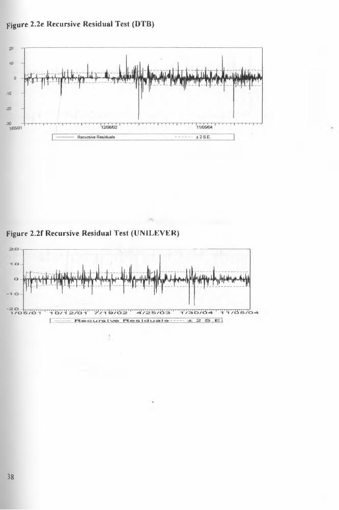
Recursive Least SquaresThis method involves estimating the price equation repeatedly using larger samples.

Recursive residuals are plotted about the zero line after estimation. Residuals outside the

standard error band suggest instability o f returns.

2.2.3 Test for volatilityConceptually, there are infinite types of non-linear models in economics; however, only a

few may be applicable in finance. The most popular of these are the ARCH and GARCH

models.

The ARCH Model

Until the ground breaking seminal paper by Engel (1982), most macro-econometrics and

financial modeling centered on conditional first moments. The importance of risk and

uncertainty however necessitated the development of alternative modeling. Engel (1982)

introduced ARCH model, whose insight is the distinction between the conditional

variances and co-variances. ARCH model has been improved upon further by many

scholars to what may be referred to as the ARCH family of models.

The ARCH (Autoregressive Conditional Heteroskedasticity) models are designed to

model and forecast conditional variances as a function of past values of the dependent

variable and independent or exogenous variables. ARCH evolved from two equations as

follows:

where equation (2.9) is the conditional mean equation which describes how the

(2.9)i= l

a'~ = a o + YjClifx-i ( 2 . 10)

dependent variable varies over time. The form it takes depends on the theory governing

the relationship between the variables specified in the model. Equation 2.10 is the

conditional variance equation.

18

In the literature, conditional variance (a ,") is referred to ash, ; hence equation 10

becomes:T

ht = a0+ Y a^ 2‘-‘ (2-11)1=1

Where h, must be strictly positive. This is referred to as the non-negativity condition.

The ARCH model has important features, which make it appropriate for financial time

series analysis. First, it takes account of volatility clustering (the tendency of large

changes to follow large changes and small changes to follow small changes). Second, it

takes care of heteroskedasticity. ARCH models however have three limitations. First, it is

problematic settling on the lag length. Second, if the lag length is big, then the model

may not be parsimonious. Lastly the non-negativity condition may be violated.

GARCH Models

The terminology stands for Generalized Autoregressive Conditional Heteroskedasticty. It

addresses the limitations of ARCH. The original GARCH model was developed

independently by Bollerslev (1986) and Taylor (1986) as a generalized form of ARCH. It

explains variance by two sets of distributed lags, one on past residual to capture high

frequency effects, and the second in lagged values of the variance itself to capture long

term effects. The generalized version of the model, known as GARCH (q,p) is given as:

+YPj°2‘-f (2. 12).=i j=\

\

This generalized GARCH model is hard to fit if more than one lag is anticipated. The

most popular model in this class is GARCH (1, 1), which is given as:

<y\ = a + axff t-\ + (2.13)

GARCH (1,1) is parsimonious, can account for both leptokurtosis and volatility

clustering and hence it is superior to the ARCH model. The major shortcoming of the

GARCH model is that the use of variance and squared errors limits all the variables to

positive values, thus implying that impact is independent of sign. Studies have shown that

in finance, negative shocks are more persistent than positive ones. In addition, it may also

19

not satisfy the non-negativity condition Because of the aforesaid problems, there is need

to address the asymmetry problem.

Asymmetric ARCH Models

This class of models takes into account the fact that downward movements in the market

are followed by higher volatilities than upward movements of the same magnitude. In

technical terms, they factor in leverage. The two main models at issue here are TGARCH

and EGARCH models.

TGARCH Model

TGARCH is a variation of GARCH introduced independently by Zakoian (1990) and

Glosten, Jaganathan and Runkle (1993). It is sometimes referred to as GJR. In this model,

the impact of good new (e,<0) and bad news (et>0) is tested to show if there is a different

impact on conditional variance of news, depending on whether downward movements in

the market are followed by higher volatilities than upward movements of the same

magnitude. The conditional variance is modeled as:

a 2t = co + a e2t-\ + J3o2t-1 + (2.14)

Where y is leverage effect and = 1 if < 1 and 0 otherwise.$

EGARCH Model

EGARCH is an acronym for exponential GARCH proposed by Nelson (1991). It

accounts for asymmetry by introducing the logarithm of conditional variances. It is givenas:

ycrVih - i | [2 (2.15)

Apart from taking into account leverage, .this model does not require non-negativityconstraint.

20

Data and estimation methods

Data was drawn from the Nairobi Stock Exchange. It covers five years between 2001 and

2005. To capture the entire sections of the market, only firms included in the computation

of Nairobi Stock Exchange index (NSE-20 Share index) are included in the sample. One

firm, Uchumi supermarkets, is however excluded since it had been suspended from stock

market at the time of this study.

An interesting but uncommon case is when change in share price is indicated as zero.

This may imply two scenarios as follows: one that there was no trading at all, and second

that trading occurred at constant prices. In an emerging market, where thin trading is

common, for simplicity and without loss o f generalization, we assume no trading.

Presented in the ensuing section are results derived from several methodologies, which

include graphical, algebraic, and regression methods.

Table 2.1 Trading characteristics of the selected firms in NSE

for the period 2001-2005

Name of Firm Comparing Trading and

Non-trading days for the data period

Bamburi Non-trading days> Trading days

Barclays Trading days> non-trading days

BAT Trading days> non-trading days

BOC Non-trading days> Trading daysDTB Non-trading days> Trading days

EABL Trading days> non-trading days

Firestone Trading days> non-trading days

G.Williamson Trading days> non-trading daysKakuzi Non-trading days> Trading days

Kenya Airways Trading days> non-trading daysKCB Trading days> non-trading days

21

Table 2.1 continued

KPLC Trading days> non-trading days

NMG Trading days> non-trading days

NIC Trading days> non-trading days

Sasini Non-trading days> Trading days

Stanchart Trading days> non-trading days

Total Trading days> non-trading days

TPS Trading days> non-trading days

Unilever Non-trading days> Trading days

2.3 Empirical ResultsThis section presents descriptive characteristics and the results of linearity and volatility

tests. The descriptive statistics are in section 2.3.1 and the estimation results in section

2.3.2.

2.3.1 Descriptive ResultsIntroduction '

t

In this section the characteristics of the share price data are explained using graphical

presentation of daily compounded percentage changes in share prices for all the selected

firms. Descriptive statistics, such as arithmetic mean, range and kurtosis are also

presented. *

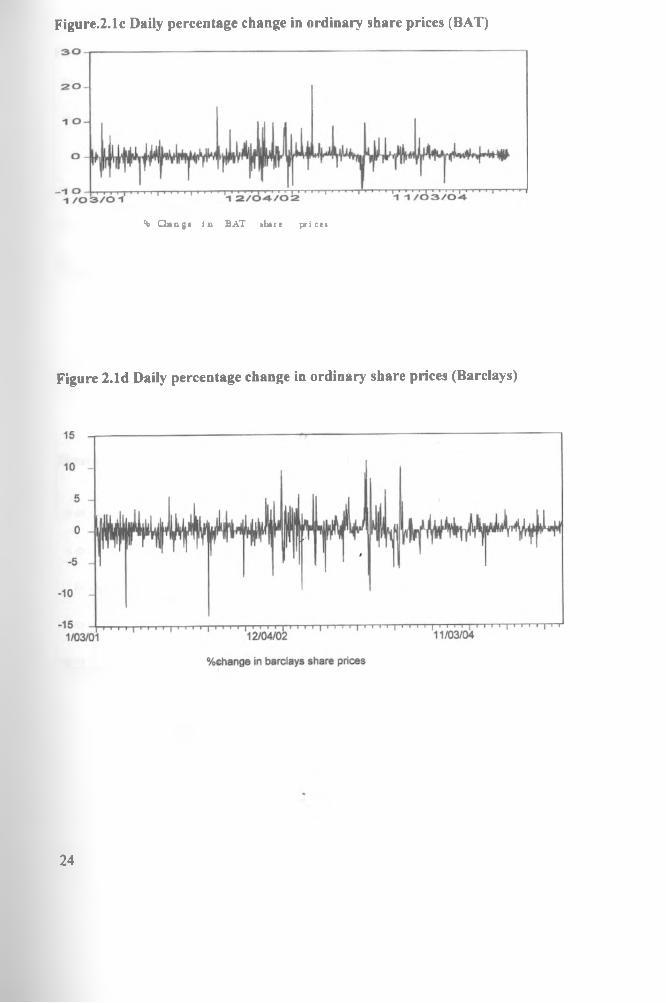
In all the graphs, the vertical axis represents percentage change in daily share prices. On

the horizontal axis, is presented the time period between 1st January 2001 and 31st

December 2005. In all the cases, extreme values (>50%) have been excluded and this

affects the variability of returns shown in the graphs.

22

Figure.2.1a Daily percentage change in ordinary share prices (Bamburi)

Figure.2.1b Daily percentage change in ordinary share prices (BOC)

-I <51 O -

-1 O

1 /O

J ..................... I i i l l i U a(l ■ "mi i I ' m * ' 1! 1 ii| 1 i n l1 nil ' r T

% Change i n BOC share p r ices

23

Figure.2.1c Daily percentage change in ordinary share prices (BAT)

% Change i n BAT share p r ices

Figure 2.1d Daily percentage change in ordinary share prices (Barclays)

24

Figure 2.1e Daily percentage change in ordinary share prices (DTB)

Figure 2.1f Daily percentage change in ordinary share prices (Unilever)

25

Figure 2.1 g Daily percentage change in ordinary share prices (EABL)

30

2 0 -

1 O

-2 0 1 /o = 3 /o i ' i O /'-i d /O V " ' " " TV I V /0 2

Change i n EABL there price*

-4/2 3/0 :

Figure 2.1h Daily percentage change in ordinary share prices (George Williamson)

% Change i n G. W i l l i a m s o n ihare price*

26

Figure 2.1i Daily percentage change in ordinary share prices (Kakuzi)

20

11 o o

-1 o-

h ld . l l1 ll|i i jiUii

% Change i n Kakuzi share p r ices

Figure 2.1 j Daily percentage change in ordinary share prices (KCB)

27

Figure 2.1k Daily percentage change in ordinary share prices (Kenya Airways)

Figure 2.11 Daily percentage change in ordinary share prices (KPLC)

28

Figure 2.1m Daily percentage change in ordinary share prices (NIC)

1/03/01 11/03/04

% change In nic share prices

Figure 2.1 n Daily percentage change in ordinary share prices (Nation)

% Change I n N a t i o n share p r ices

29

Figure 2.1o Daily percentage change in ordinary share prices (Sasini)

2 ° t 1 S -

% Change I n S a s t n i ihare p r ices

Figure 2.lp Daily percentage change in ordinary share prices (Total Kenya)

% Gian ge i n Total share p r ices

30

Figure 2.1 q Daily percentage change in ordinary share prices (Firestone)

Figure.2.1 r Daily percentage change in ordinary share prices (TPS)

Figure 2.1s Daily percentage change in ordinary share prices (STANCHART)

From the graphs it can be noted that there are no wild swings but rather a cluster of changes seemingly similar in magnitude. Big changes tend to follow big ones and small ones tend to follow small changes. This evidence suggests that there is volatility clustering in the share price data.

31

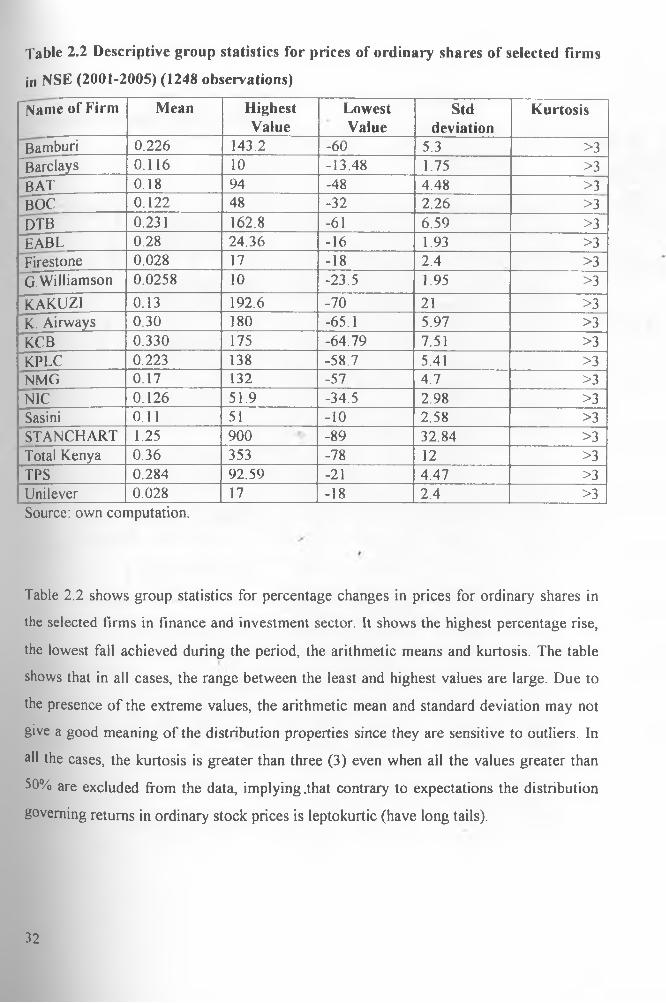
Table 2.2 Descriptive group statistics for prices of ordinary shares of selected firms

in NSE (2001-2005) (1248 observations)

"Name of Firm Mean HighestValue

LowestValue

Stddeviation

Kurtosis

Bamburi 0.226 143.2 -60 5.3 >3"Barclays 0.116 10 -13.48 1.75 >3BAT 0.18 94 -48 4.48 >3BOC 0.122 48 -32 2.26 >3DTB 0.231 162.8 -61 6.59 >3EABL 0.28 24.36 -16 1.93 >3Firestone 0.028 17 -18 2.4 >3G.Williamson 0.0258 10 -23.5 1.95 >3KAKUZI 0.13 192.6 -70 21 >3K. Airways 0.30 180 -65.1 5.97 >3KCB 0.330 175 -64.79 7.51 >3KPLC 0.223 138 -58.7 5.41 >3NMG 0.17 132 -57 4.7 >3NIC 0.126 51.9 -34.5 2.98 >3Sasini 0.11 51 -10 2.58 >3STANCHART 1.25 900 -89 32.84 >3Total Kenya 0.36 353 -78 12 >3TPS 0.284 92.59 -21 4.47 >3Unilever 0.028 17 -18 2.4 >3Source: own computation.

Table 2.2 shows group statistics for percentage changes in prices for ordinary shares in

the selected firms in finance and investment sector. It shows the highest percentage rise,

the lowest fall achieved during the period, the arithmetic means and kurtosis. The table

shows that in all cases, the range between the least and highest values are large. Due to

the presence of the extreme values, the arithmetic mean and standard deviation may not

give a good meaning of the distribution properties since they are sensitive to outliers. In

all the cases, the kurtosis is greater than three (3) even when all the values greater than

50% are excluded from the data, implying .that contrary to expectations the distribution

governing returns in ordinary stock prices is leptokurtic (have long tails).

32

2.3.2. Linearity test results

Table 2.3 RESET Results for selected firms in NSE. (1248 observations) Dependent variable: G R O W T H P R I C E __________________Firm Variable Coefficient Std.

Error/-

StatisticProb. /rvalue for

loglikelihood

ratiob a m b u r i C 0.033947 0.058485 0.580445 0.5617 0.01

GROWTHINDEX 0.791927 0.075905 10.43308 0.0000FITTEDA2 0.118260 0.043487 2.719468 0.0066

Tu t C -0.023704 0.056628 -0.41859 0.6756 0.00GROWTHINDEX 0.860247 0.072665 11.83847 0.0000

FITTEDA2 0.150941 0.033654 4.485032 0.0000b a r c l a y s C 0.025689 0.048650 0.528025 0.5976 0.02


BOC C 0.067848 0.046336 1.464273 0.1434 0.17GROWTHINDEX 0.230861 0.064276 3.591720 0.0003

FITTEDA2 0.457797 0.330478 1.385258 0.1662UNILEVER C -0.111327 0.076239 -1.46023 0.1445 0.00


DTB C -0.021228 0.077960 -0.27229 0.7854 0.15GROWTHINDEX 1.015607 0.098712 10.28854 0.0000

FITTED A2 0.055769 0.039229 1.421631 0.1554EABL C 0.216721 0.062918 3.444515 0.0006 0.00

GROWTHINDEX 0.376331 0.078522 4.792656 0.0000FITTED A2 0.033699 0.007252 4.646874 0.0000

NIC C -0.070383 0.067040 -1.04985 0.2940 0.00GROWTHINDEX 0.904431 0.085449 10.58449 0.0000

FITTEDA2 0.181947 0.033705 5.398241 0.0000G.Williamson C -0.057630 0.056964 -1.01168 0.3119 0.00

GROWTHINDEX 0.764833 0.092115 8.303053 0.0000FITTEDA2 0.312724 0.107932 2.897418 0.0038FITTEDA3 -0.226081 0.064035 -3.53059 0.0004

Kakuzi C -0.066988 0.070163 -0.95475 0.3399 0.03GROWTHINDEX 0.774223 0.088006 8.797415 0.0000

FITTEDA2 0.123937 0.057956 2.138481 0.0327KenyaAirways

C 0.125403 0.072484 1.730072 0.0839 0.30GROWTHINDEX 0.960966 0.095424 10.07048 0.0000

FITTEDA2 0.042306 0.040567 1.042865 0.2972

33

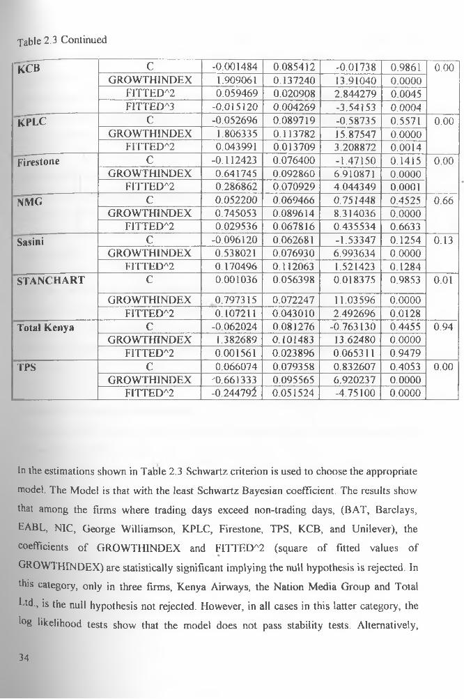
Table 2.3 Continued

1CCB C -0.001484 0.085412 -0.01738 0.9861 0.00GROWTHINDEX 1.909061 0.137240 13.91040 0.0000

FITTEDA2 0.059469 0.020908 2.844279 0.0045FITTEDA3 -0.015120 0.004269 -3.54153 0.0004

Tcplc C -0.052696 0.089719 -0.58735 0.5571 0.00GROWTHINDEX 1.806335 0.113782 15.87547 0.0000

FITTEDA2 0.043991 0.013709 3.208872 0.0014Firestone C -0.112423 0.076400 -1.47150 0.1415 0.00


NMG C 0.052200 0.069466 0.751448 0.4525 0.66GROWTHINDEX 0.745053 0.089614 8.314036 0.0000

FITTEDA2 0.029536 0.067816 0.435534 0.6633Sasini C -0.096120 0.062681 -1.53347 0.1254 0.13


STANCHART C 0.001036 0.056398 0.018375 0.9853 0.01


Total Kenya C -0.062024 0.081276 -0.763130 0.4455 0.94GROWTHINDEX 1.382689 0.101483 13.62480 0.0000

FITTEDA2 0.001561 0.023896 0.065311 0.9479TPS C 0.066074 0.079358 0.832607 0.4053 0.00

GROWTHINDEX '0.661333 0.095565 6.920237 0.0000FITTEDA2 -0.244791 0.051524 -4.75100 0.0000

In the estimations shown in Table 2.3 Schwartz criterion is used to choose the appropriate

model. The Model is that with the least Schwartz Bayesian coefficient. The results show

that among the firms where trading days exceed non-trading days, (BAT, Barclays,

EABL, NIC, George Williamson, KPLC, Firestone, TPS, KCB, and Unilever), the

coefficients of GROWTHINDEX and FITTEDA2 (square of fitted values of

GROWTHINDEX) are statistically significant implying the null hypothesis is rejected. In

this category, only in three firms, Kenya Airways, the Nation Media Group and Total

Ltd., is the null hypothesis not rejected. However, in all cases in this latter category, the

log likelihood tests show that the model does not pass stability tests. Alternatively,

34

among firms where non-trading days exceed trading days (BOC, DTB, and Sasini), the

results show that the null hypothesis is rejected. These entire firms share a common

characteristic, i.e., the non-trading days exceed the trading days by a large margin. Again

in this category, two firms where the non-trading days exceed the trading ones by a small

margin, the results show that the null hypothesis is rejected. However, the log likelihood

tests show that the model does not pass stability test.

Similar results are obtained when all the firms considered are stacked together to form

one big pool representing all listed firms. Second, the quadratic functional form fits the

data best for most firms. The quadratic form shows that the relationship between returns

on ordinary share prices and returns on market index is not effectively represented by a

linear function.

It can be pointed out that the contradictions to this finding can partly be attributed to thin

trading which in turn can lead to instability in a stock market. It is evident that in all the

cases, where the null hypothesis was not rejected, the log likelihood test showed that the

model was unstable implying that the linearity could not hold with added or reduced

sample size.

Recursive Residual Test ResultsThe graphs show results for all the nineteen (19) of the twenty (20) firms used in the

computation of NSE-20 index.

UNIVERSIT Y OF ft AlRQRi LIBRARY

35

Figure 2.2a Recursive Residual Test (BAMBURI)

Figure 2.2b Recursive Residual Test (BOC)

1 /OS/O 1 1 2 /3 e /o 5R e o u rs i v e R e s i d u I s

i T/os/cT*=fc 2 - E l

36

Figure 2.2c Recursive Residual Test (BAT)

Figure 2.2d Recursive Residual Test (BARCLAYS)

Recursive Residuals ------------± 2 S.E.

37

Figure 2.2e Recursive Residual Test (DTB)

Figure 2.2f Recursive Residual Test (UNILEVER)

-2 O-I / O S / O -1

38

Figure 2.2g Recursive Residual Test (EAST AFRICAN BREWERIES)

Figure 2.2h Recursive Residual Test (GEORGEWrLLIAMSON)

39

Figure 2.2i Recursive Residual Test (KAKUZ1)

Recursive Residuals 2 S.e]

Figure 2.2j Recursive Residual Test (KCB )

----------- Recursive Residuals ------------ ± 2 S.E.

40

Figure 2.2k Recursive Residual Test (KENYA AIRWAYS)

Recursi ve Resid uala--------± 2 S . E (.

Figure 2.21 Recursive Residual Tests (KENYA POWER AND LIGHTING)

Recursive Residuals--------± 2 S.e|

41

Figure 2.2m Recursive Residual Test NIC

Figure 2.2n Recursive Residual Test (NATION)

42

jU

Figure 2.2o Recursive Residual Test (SASINI)

1 /O 5/0 1 1 2/06/02

---------- Recursive Residuals

1 1 /O 5/0*4

t, 2 s Te !

Figure 2.2p Recursive Residual Test (TOTAL KENYA)

2 0

Figure 2.2q Recursive Residual Test (FIRESTONE)

20

1 ' ' " i ’o / ̂ '^ / O '-i' ' "71 /2 4 /2) 2 ' ' - 4 / 2 9 7 6 3 ' ' " 2/0 1 ’ ' " i ' T / c i ' / /O -4■ ■ ■ Rec t_j ns i ve R e s idua la -------- ± 2 S

43

Figure 2.2r Recursive Residual Test (TPS)

Figure 2.2s Recursive Residual Test (STANDARD CHARTERED)

From the graphs, it can be noted that for all the firms several residuals are outside the 5%

significance band indicating that there is parameter variance instability in the residuals

suggesting the presence of volatility. This is also true when all the firms are put together

Considered together, RESET and recursive residual tests confirm that though, generally,

linear relationship may not truly represent the behavior between returns on ordinary share

prices and the market index, individual firms may yield different results. These results

may be attributed to frequency of trading of shares in the market and to internal

characteristics of firms. It may be important to point out that it is in firms characterized

by thin trading that the difference is noted. Still, linearity cannot be rejected in these latter

cases. The linear model is shown to be unstable, which supports the conclusion that this

model is not appropriate.

44

2.3.3 Volatility Test ResultsThis section presents and compares results from the various ARCH family of models.

The equation associated with each table of results is repeated for ease of interpretation of

results.

GARCH (1,1)To recapitulate, the GARCH (1,1) equation estimated is

cr2( = (0 + a xf/ t-1 + Pxcr2t-\

(See equations 2.9 and 2.10 for computation of a 2, and ju2t-i )

Where a and, (3 are ARCH effects. If a + 3 is close to unity (1), then volatility persists.

Table 2.4 GARCH (1, 1) results for selected firms in NSE (1248 observations)* ~

Dependent variable: Conditional Variance (cr"t)FIRM Coef P-

value

DIAMOND TRUST BANKa 0.11 0.00**3 0.84 0.00**

(a+ p ) (L95 -

KCBa 0.23 0.00**3 0.75 0.00**

(a + 3 ) 0.98 -

NICa 0.07 0.00**P 0.89 0.00**

(a + 3 ) 0.96 -

BARCLAYSa 0.25 0.00**3 0.70 0.00**

(a + 3 ) 0.95 -

b a m b u ri a 0.05 0.00**P 0.89 0.00**

(a+p) 0.94 -

BOC a 0.03 0.00**P 0.95 0.00*

(a+ P ) 0.98 -

45

Table 2.4 Continued

bat a 0.25 0.00**P 0.59 0.00**

-M P ) 0.84 -

UNILEVER TEAa 0.14 0.00**

— El . 0.83 0.00**(a+P) 0.94 -

EABLa 0.06 0.00**P 0.88 0.00**

(a+P) 0.95 -

GEORGE WILLIAMSONa 0.11 0.00**P 0.72 0.00**

(a+P) 0.83 -

KAKUZ1a 0.09 0.00**P 0.87 0.00**

(a+P) 0.96 -

KENYA AIRWAYSa 0.32 0.00**P 0.59 0.00**

(a+P) 0.91 -

KPLC a 0.05 0.00**P 0.93 0.00**

(a+P) 0.98 -NATION MEDIA a 0.40 0.00**

P 0,32 0.00**(a+P) 0.72

SASINI a 0.34 0.00**P 0.35 0.00**

(a+P) 0.69 -

TOTAL KENYAt

a 0.16 0.00**P 0.62 0.00**

(a+p) 0.78 -

FIRESTONE a 0.14 0.00**P 0.83 0.00**

(a+P) 0.97 -

TPS a 0.04 0.00**P 0.96 0.00**

(a+P) 1.00 -

STANDARD CHARTERED

--- ------------------------------

a 0.32 0 00**P 0.53 0.00**

(a+P) 0.85 -

Indicates rejection of null hypothesis at better than 5% level.

46

The results in Table 2.4 show that in all the cases a + (3 is close to unity (1), suggesting

that volatility persists. Hence we can confirm that there is ARCH effect in all firms in

finance and investment sector.

TGARCH

The conditional variance equation estimated under TGARCH model is (2.14)

a 2, = a> + a e 2,-\ + J3cr2,-1 + y i? t- \I t_x

Where y is leverage effect and = 1 if /it_x < 1 and 0 otherwise. p,.|<l is considered

good news while p(.it>0 represents bad

Table 2.5 TGARCH results for selected firms in NSE (1248 observations) Dependent variable: Conditional Variance ( a 2i )FIRM Coef p-valueBAMBURI a 0.06 0.00**

Y -0.03 0.01**

JJ 0.89 0.00**BARCLAYS a 0.35 0.00**

Y -0.21 0.00**P 0.72 0.00**

BOC a 0.03 0.00**Y ■ p b "A 0.00**P 0.95 0.00**

BAT a 0.29 0.00**Y -0.07 0.01**P 0.58 0.00**

DIAMOND TRUST BANKt

a 0.12 0.00**Y -0.02 0.00**P 0.84 0.35

UNILEVER TEA a 0.18 0.00**Y -0.14 0.00**P 0.86 0.00**

EAST AFRICAN BREWERIES a 0.09 0.00**Y -0.05. 0.03**P 0.89 0.00**

47

Table 2.5 Continued

GEORGE WILLIAMSON a 0.11 0.00**r - 0.009 0.67

P 0.71 0.00**

KAKUZ1 a 0.12 0.00**Y - 0.10 0. 00* *

0.87 0.00**KENYA AIRWAYS a 0.37 0.00**

r - 0.18 0. 00* *

P 0.63 0.00**KCB a 0.31 0.00**

r - 0.16 0. 00* *

p 0.75 0.00**KENYA POWER AND LIGHTING a 0.06 0.00**

Y - 0.03 0. 00* *

P 0.93 0.00**NATION MEDIA a 0.90 0.00**

Y - 0.83 0. 00* *

P 0.33 0.00**NIC a 0.10 0.00**

Y - 0.03 0. 00* *

P 0.89, 0.08SASINI a 0.37 0.00**

Y - 0.08 0.20

P 0.36 0.00**TOTAL KENYA a 0.37 0.00**

Y - 0.37 0. 00* *

P 0.61 0.00**FIRESTONE a 0.18 0.00**

Y - 0.14 0. 00* *

P 0.86 0.00**TPS a 0.05 0.00**

r - 0.03 0 . 00* *

P 0.97 0.00**STANDARD CHARTERED a 0.33 • 0.00**

Y - 0.03 0.300.55 0.00**

** Indicates rejection of null hypothesis at 5% level.

48

The results in Table 2.5 show that for the firms the coefficient representing leverage

effect (y) are significantly different from zero thus confirming the presence of asymmetry

in the firms included in NSE 20 index. The same can be said for the entire market. In

addition the same coefficient is negative implying that there is evidence of asymmetry

and that bad news (negative changes in stock prices) tend to lead to more persistent

volatility than good news (positive changes in stock prices).

e g a r c h

The conditional variance equation estimated is (2.15)

Table 2.6 EGARCH results for selected firms in NSE

(1248 Observations)Dependent variable: Log of Conditional Variance ln( a 2, )FIRM Coef

s'

p-value

BAMBURI a 0.13 ' 0.00**P -0.01 0.27

Y 0.95 0.00**BARCLAYS a 0.33 0.00**

P 0.93 0.00**Y 0.10 0.00**

BOC a 0.13 0.00**P 0.03 0.00**

Y 0.94 0.00**BAT a 0.37 0.00**

P 0.03 0.02**

J L 0.80 0.00**

49

Table 2.6 Continued

Diamond Trust Bank a 0.07 0.00**_P_ 0.92 0.00**JL_ 0.07 0.57

UNILEVER TEA a 0.27 0.00**0.07 0.00**

JL_ 0.93 0.00**EAST AFRICAN BREWERIES a 0.18 0.00**

J_, -0.06 0.00**Y 0.92 0.00**

GEORGE WILLIAMSON a 0.23 0.00**P 0.028 0.04**Y 0.79 0.00**

KAKUZ1 a 0.20 0.00**P 0.04 0.00**Y 0.93 0.00**

KENYA AIRWAYS a 0.50 0.00**J _ 0.09 0.00**Y 0.85 0.00**

KCB a 0.30 0.00**J _ 0.91 0.00**Y 0.06 0.00**

KENYA POWER AND LIGHTING a 0.12 0.00**P 0.04' 0.00**Y 0.97 0.00**

NATION MEDIA a 0.50 0.00**0.37 0.00**

_Y_ 0.63 0.00**

SO

Table 2.6 Continued

NIC a. 0.14 0.00**0.97 0.00**

JL. 0.01 0.57SASrN l a 0.43 0.00**

0.03 0.17

JL j 0.63 0.00**T o ta l Ke n y a a 0.23 0.00**

P 0.23 0.00**J L 0.77 0.00**

f ir e s t o n e a 0.27 0.00**P 0.07 0.00**

1 0.93 0.00**TPS a 0.098 0.00**

P 0.03 0.00**0.99 0.00**

STA N D A RD C H A R T E R E D a 0.29 0.00**P 0.05 0.00**Y 0.93 0.00**

** Indicates rejection of null hypothesis at 5%

The results in Table 2.6 show that in 16 outfifthe 19 firms considered, all the»

coefficients (a,p,y) are significantly different from zero indicating that the null

hypothesis is rejected. This indicates the presence of leverage effect, confirming the

asymmetry of variance of share return.

From both Tables 2.5 and 2.6 we note that though the TGARCH and EGARCH models

do not give identical results in terms of coefficients, their interpretation is similar to that

of the pattern in changes in ordinary share prices, as both indicate existence of

asymmetry in the variance of returns.

51

Though results from certain firms are conflicting, on average they show the following:

First, that the distribution of returns on ordinary share prices is leptokurtic (have long

tails) as demonstrated by the large kurtosis. This is contrary to findings in some of the literature.

Second, the linear model fails to capture the relationship between returns on ordinary

share prices and the market share index. The model that seems to fit the data best is:

!(,=& + P\Rm, + P2̂ ~m< + £t

Third, there is evidence of volatility clustering in stock returns and, by extension, prices.

This implies that though big changes tend to follow big changes and vice versa, there is

no evidence of price predictability since the presence of ARCH effect confirms volatility

in the stock market.

Fourth, that there is evidence of asymmetry in returns on ordinary shares, implying that

most investors are in the secondary markets, where they put in money with the aim of

benefiting from changes in share prices rather than from dividends.t

Fifth, that TGARCH is a better method for modeling conditional variance since though

its results are not very different from EGARCH ones, the former displays asymmetry in

that a decrease in stock prices is more likely to trigger further rapid decreases than ant

increase in prices. This suggests that most investors in the market are more sensitive to a

price fall than to a price increase. The possible explanation for this is that an increase in

price is viewed as an opportunity to make more profit so that investors tend to hold on to

shares with the expectation of making windfall gains. Alternatively, a fall in prices is met

with panic selling, thus reducing prices further. Lastly, individual characteristics of the

firm seem to play an important role in the response of firms to stock market conditions,

and in modeling stock market behavior, since not all firms behave similarly.

2.4 Conclusion

52

REFERENCES

Anthony, L. (2006), “Testing Stock Market Efficiency Hypothesis in Tanzania,”

unpublished M.A. (Economics) Thesis, University of Dar es Salaam.

Aggarwal, R., Prabhala, N.R. and Puri, M. (2002), “Institutional Allocation of Initial

Public Offerings: Empirical Evidence,” Journal o f Finance , 52, 1421-1442.

Ball, R. and Brown, P. (1968), “An Empirical Evaluation of Accounting Income

Numbers,” Journal o f Accounting Research, 6, 159-178.

Bernard, V. and Thomas, J. (1990), “Evidence that Stock Prices do not Fully Reflect the

Implications of Current Earnings for Future Earnings,” Journal o f accounting and

Economics, 13, 305-340.

Black, F. (1972), “Capital asset Equilibrium with Restricted Borrowing,” Journal o f

Business, 45, 29-44./'

0Bollerslev, T. (1986) “Generalized Autoregressive Conditional Heteroskedasticity,”

Journal o f Econometrics, 31, 307-327.

Bollerslev, T. and Hodrick, R.J. (1992), “Financial Market Efficiency Tests,” NBERWorking Papers Series no. 4108.

Brav, A. and Gompers, P. (1997), “Myth or Reality? The Long-Term Underperformance

of Initial Public Offerings. Evidence from Venture and Non-venture Capital-

Backed Companies,” Journal o f Finance, 52, 1791-1820.


Financial Economics, 6, 307-17.

Brooks, C., Rew, A.G., and Ritson, S. (2001), “A Trading Strategy Based on the Lead-

Lag Relationship Between the FTSE 100 Spot Index And the LIFFE Traded FTSE

Futures Contract,” Journal o f Forecasting, 17, 31-44.

Brooks, C. (2004), Introductory Econometrics for Finance, London: Cambridge

University Press.

Brown, S. J, and Warner, J.B. (1980), “Measuring Security Price Performance,” Journal

o f Financial Economics, 8, 205-258.

Brown, S. J, and Warner, J.B. (1985), “Using Daily stock Returns: The case of Event

Studies,” Journal o f Financial Economics, 14 3-31.

Campbell, J. Y., Lo, A.W., and MacKinlay, AC. (1997), The Econometrics o f Financial

Markets, Princeton, New Jersey: Princeton University Press.

Corrado, C. J. and Zivney, T.L. (1992), “The Specification and Power Sign test in Event

Study Hypothesis Tests Using Daily Stock Returns,” Journal o f Financial and

Quantitative Analysis, 27, (3), 465-471

Cowles, A. (1960), “A Revision of Previous conclusions regarding Stock Price

Behavior,” Econometrica, 28, 909-15.

kDeBondt, W. F. M. and Thaler, R.H. (1985), “Does Stock Market Overreact?,” Journal o f

Finance, 40, 793-805.

DeBondt, W. F. M. and Thaler, R.H. (1987), “Further Evidence on Investor Overreaction

and Stock Market Seasonality,” Journal o f Finance, 42, 567-80.

54

De Jong, F., Kemna, A. and Klock, T. (1992), “A contribution to Event Study

Methodology with an Application to Dutch Stock Market,” Journal o f Banking

and Finance, 16, 11-36.

Diebold, F. X. and Kamil, Y. (20U9), “Measuring Financial Asset Return and Volatility

Spillovers, with Application to Global Equity Markets,” Economic Journal, 119,

158-171.

Engel, R. (1982) “Autoregressive Conditional Heteroscedasticity with Estimates of the

Variance of United Kingdom Inflation,” Econometrica, 50 (4), 987-1007.

Engel, R. and Kroner, K. (1995) “Multivariate Simultaneous Generalized ARCH,” Engel,

R. (2002), “New Frontiers for ARCH Models,” Journal o f Applied Econometrics

,17, 425-446.

Fama, E. F., (1970), “Efficient capital markets: a review of theory and empirical work,”

Journal o f Finance, 25, 383-417.

Fama, E. F. (1998), “Market efficiency, Long-term .Returns, and Behavioral Finance,”

Journal o f Financial Economics 41, 283-306.

Fama, E. F., French, K. (1992), “The Cross-section of Expected Stock Returns,” Journal

o f Finance, 41, 427-465,

Figlewski, S. (2004), “Forecasting Volatility,” Draft paper, New York University Stem

school of Business, April 2004.

Glosten, L. R., Jagannathan, R. and Runkle, D.E. (1993), “On Relation Between the

Expected Value and the Volatility of Nominal Excess Returns on Stock,” The

Journal o f Finance, 48, (5), 1979-1801.

55

Granger, C. W. J. (1992), “Forecasting Stock Market Prices: Lessons for Forecasters,”

International Journal o f Forecasting, 8, 3-13.

Hinich, M. J. and Patterson, D M. (1995), “Evidence of Nonlinearity in Daily Stock

Returns,” Journal o f Business and Economic Statistics, 3(1), 69-77

Ho, K. (2004), “Modeling Long Memory and Asymmetry in Exchange Rate Volatility: A

multi GARCH approach With Time-Varying Correlation,” Unpublished Paper,

Department of Economics, Cornell University and Department of economics,

National University of Singapore.

Hsieh, D. A. (1989), “Testing Nonlinear Dependence in Daily Foreign exchange Rates,”

Journal o f Business, 62, (3), 339-68. Ibbotson, R. (1975), “Price Performance of

Common Stock New Issues,” Journal o f Financial Economics, September, 235-

272.

Ibbotson, R. (1975), “Price Performance of Common Stock New Issues” Journal o f

Financial Economics, September, 235-272. ,

Ibbotson, R. and Jaffe, J .F. (1975), “Hot Issue” Markets,” Journal o f Finance, 30, 1027-

1042.

»

Jegadeesh, N. and Titman, S. (1993), “Return of Buying Winners and Selling Losers:

Implications for Stock Market Efficiency,” Journal o f Finance , 48, 65-91.

Jegadeesh, N. and Titman, S. (2001), “Profitability of Momentum Strategies: An

Evaluation of Alternative Explanations,” Journal o f Finance, 56, 699-720.

Kim, E. H. and Singal, V. (2000), “Stock Market Openings: Experience of Emerging

Markets,” Journal o f Finance, 73, (1), 25-66.

56

Kothari, S. P. and Warner, J.B (2004), in Eckpo, B E. (Eds) Handbook o f Corporate

Finance: Empirical Corporate Finance, Elsevier/North-Holland.

Koulakiotis, A., Papasyriopoulus, N., and Molyneux, P (2006), “More Evidence on the

Relationship between Stock Price Returns and Volatility. A Note,” International

Research Journal o f Finance and Economics, issue 1.

Kxitzman, M. P. (1994), “About Event Studies,” Financial Analysts Journal, 50, 17-20.



Laughran, F. and Ritter, J. (1995), “New Issues Puzzle,” Journal o f Finance, 50, (1), 23-

51.

Lee, I (1994), “Do Firms Knowingly Sell Overvalued Equity?,” Working Paper,

University of Illinois.

LeRoy, S. (1973), “Risk Aversion and the Martingale Property of Stocks Returns,”

International Economic Review, 14, 436-46.

i

Lucas, R. (1978), “Asset Prices in Exchange Economy,” Econometrica, 46, 1429-46.

Mackinlay, AC. (1997), “Event Studies in Economics and Finance,” Journal o f

Economic Literature, 35,(1), 13-39.

Nelson, D. B. (1991), “Conditional Heterescedasticity in Asset Returns: A New

Approach,” Econometrica, 59, 347-370.

57

jsjgugi, R. W., Murinde, V. and Green, C.J. (2005), in Green, C.J., Kirkpatrick, C.H. and

Murinde, V. (eds) Finance and Development Surveys o f Theory, Evidence and

Policy, Edward Eiger, Cheltenham, UK.

NSE (2005), Handbook, Nairobi Stock Exchange, Nairobi, Kenya

Osborne, M. F. (1964), “Brownian Motion in Stock Market, in P. Cooter ed, Ihe Random

Character o f Stock Market Prices, Cambridge. MIT Press

Pesaran, M. H. (2005), “Market Efficiency Today,” IEPR (University of Southern

California) Working Paper 05.41.

Pesaran, M. H. and Timmermann, A. (1995), “The Robustness and Economic

Significance of Predictability of Stock Returns,” Journal o f Finance, 50, 1201-

1220.

/Pesaran, M. H. and Timmermann, A. (1994), “Forecasting Stock Returns. An

Examination of Stock Trading in the Presence of Transaction Costs,” Journal o f

Forecasting, 13, 330-365.

Poon, S., and Granger, C. W (2003), “Forecasting Volatility in Financial Markets: A

Review,” Journal o f Economic Literature, 41, (.2), 478-539.

Pynnonen, S. and Pape, B (2005), “Non-linear Univariate Time series,” Unpublished

paper, Department of Mathematics and Statistics, University of Vasa

Ramsey, J. B. (1969), “Tests for Specification Errors in Clasical Linear Least Square

Analysis,” Journal o f Royal Statistical Society, Series B, 31 (2), 350-371

58

Reynolds, K M. (2006), “Anticipated Versus Realized Benefits: Can Event Studies be

Used to Predict Impact of New Regulations,” Working Paper Series, No. 2006-02,

Department of Economics, American University, Washington DC.

Ritter, J. (1994), “Long Run Performance of Initial Public Offerings,” Journal o f

Finance, 46, 3-28.

Ritter, J. and Welch, I (2002), “A Review of IPO Activity Pricing and Allocations,”

Journal o f Finance, 5, 7 (4), 1794-1828.

Rubinstein, M. (1976), “The Evaluation of Uncertain Income Streams of Pricing and

Options,” Bell Journal o f Economics, 7, 407-25.

Schwert, G. W. (1993), “Stock Market Volatility,” Financial Analysis Journal,

July/August.

Schwert, G. W. (1990), “Stock Market Volatility: Teri Years after the Crash,” Brookings

Wharton papers on financial services, 65-114.

Schwert, G. W. (1989), “Stock market volatility,” Financial Analysis Journal, May/June.I

Samuelson, P. (1965), “Proofs that Property Anticipated Prices Fluctuate Randomly,”

Industrial Management Review, 6, 41-49.

Taylor, S. (1986), Modeling Financial Time series, John Wiley and Sons, New York.

59

Tse, Y. K. (1995), “Lead-Lag Relationship Between Spot Index And Future Prices of

NIKKEI Stock Average,” Journal o f Forecasting, 14, 553-56.

Zakoian, J.M. (1990), “Threshold Heteroscedasticity Models,” Manuscript CREST,

INSEE, Mimeo.

60

CHAPTER THREE

Stock Market Seasonality: Evidence from NSE

3.0. IntroductionThis chapter addresses objective three of the thesis. It seeks to generate evidence on stock

market seasonality by testing the presence of calendar anomalies in Nairobi stock

exchange. The evidence would further show whether it is possible for investors to make

abnormal profits if they base their investment rules on certain days, months or particular

partitions of the year. The relevant literature is reviewed before the presentation of

estimation methods and the empirical results.

3.1 Literature ReviewAnomalies in stock markets generally refer to any occurrences that defy prevailing theory

that is used to explain such markets i.e. EMH. Calendar anomalies in stock returns on the

other hand specifically refer to the tendency of financial asset returns to display

predictable seasonality at certain days of the week, week of the month and, month of the

year This systematic pattern permits trading- strategies to earn excess profits andt

contradict efficient market hypothesis, and the claimed accuracy of the asset pricing

model. Scholars have attributed such anomalies to tax loss hypothesis, settlement

procedures, negative information releases and bid-ask spread biases (Alagidede and

Panagiodis 2006). The major calendar anomalies include January, tum-of-the-year, day-I

of- the- week, tum-of-the-month and holidays anomalies. This study however

investigates three anomalies; day-of-the-week, month-of-the-year and quarter-of-the-year

effects on stock returns.

The day-of-the-week effect states that expected returns are not the same for all

weekdays. This has been documented by many authors including Cross (1973), French

(1980), Gibbons and Hess (1981) and Keim and Stambaugh (1983) among others. The

61

Monday effect, for example, considers return for preceding trading day to Monday’s

closing. Many studies have found the Monday effect to be negative (French 1980).

Month-of-the-year effect recognizes that returns seem to have a pattern such that some

months have lower returns than others such that it is possible to achieve abnormal profits

by consistently buying or selling shares in some months than others. Of these, January

and tum-of-the-year effects are the most documented. Rozeff and Kinney (1976),

Gultekin and Gultekin (1983), Keim (1983), Givoly and Ovadia (1983) and Griffiths and

White (1993) all documented that for one reason or another stocks have a higher return in

January compared to other months.

Quarter-of-the-year effect, though not frequently encountered in the literature, allows

expected daily compounded returns to be consistently higher or otherwise on certain

quarters of the year such that an investor can take advantage of this pattern to make

abnormal profits.

Calendar anomalies have been widely studied mostly in developed markets, and have

generated an exciting literature. Alagidede and Panagiotidis (2006) investigated day of

the week and month-of-the-year effects in the .Ghanaian stock exchange using

continuously compounded daily and monthly index returns. They confirmed that stocks

exhibit lower returns over periods between Friday’s close and Monday’s close. This is

consistent with findings of Gibbons and Hess (1991), and Al-Loughani and Chappell

(2001). The Monday effect is explained by the fact that most unfavorable news tends to

occur during the weekend thus investors sell on Monday. Monday is also associated with

pessimism unlike Friday when investors are optimistic. However they found that on the

average, returns are higher in April contrary to most studies in developed markets which

point at January effect.

Schwert (2002) acknowledges that evidence on anomalies indicates that either markets

are inefficient in which case there are profit opportunities or that that there are

inadequacies in the underlying asset-pricing model. He showed that size of the firm,

62

value effect, weekend effect and dividend yield effects normally weaken and finally

disappear after the publication of the paper stating so. This he attributed to the fact that

when practitioners learn about anomalies they trade till profitable transactions vanish or

that anomalies may not have existed in the first place. He therefore asserted that

anomalies may be more apparent than real

Chia et al. (2006) studied anomaly patterns in Malaysia using Ordinary Least Squares

(OLS) and Generalized Autoregressive Conditional Heteroskedasticity (GARCH)

models. They found that using OLS, different patterns of day-of-the-week specifically

Monday and Friday effects, were revealed in the pre-crisis period even though there was,

no evidence of January or any month seasonality during both pre and post crisis periods.

They also found out that methodology plays a role in the analysis since some anomalies

become insignificant when the GARCH method is used.

Hansen et al. (2005) asserts that discovery of calendar anomalies does not mean they

actually do exist, but may be attributed to data mining. They stress their assertion by

pointing out that extensive search across a number of possible calendar effects can yield

significant results. They also noted that theoretical explanation about the said effect haves'

been suggested subsequent to empirical discovery. In their study using a robust

methodology, they found out that though end-of-the-year effect seems to be predominant,

calendar effects have been diminishing since late 1980s with the possible exception of

small-cap indices.

>

3.2 MethodologyTwo sets of methodologies are used in this chapter to study stock market anomalies. The

first is the OLS applied to data on daily compounded return in Nairobi Stock Exchange

and the market index (NSE20). The second is the ARCH family of models that take

volatility of returns into consideration. The methodologies test existence of day-of-the-

week, month-of-the-year and quarter-of-the-year effects (see Ariel, 1987; Gao and Kling,

2005; Davidson, 2006, Barone, 1989; Bachelier, 1964).

63

the leverage effect (to test for asymmetry), whose sign and statistical significance have an

implication on the impact of good news and bad news on volatilities of stock returns. The

mean equation is actually adopted from the OLS function; however, as stated in equation

2.14, the specification of this equation is

a 2t = 0) + a s 21-\ + p a 2,-1 + y/j2 t-\I t_y

Where y is leverage effect and I t_f = 1 if gt-i<l and 0 otherwise; p«-i<l is considered

good news while gt-it>0 represents bad news.

EGARCH

Exponential GARCH (EGARCH) is an asymmetric model which involves taking

logarithms of variances thus ensuring that negative values are not reported. Like all the

ARCH models, it has both the mean and variance equations Whereas the mean equation

is general, the specification for variance equation (see 2.15) is

Where a and 3 are ARCH effect, and y is leverage effect.

3.3 Data and empirical results

3.3.1 DataThis study uses daily compounded returns on Nairobi stock exchange 20 (NSE 20) index.

Since NSE 20 index is based on 20 most traded firms from the Nairobi stock Exchange, it

gives a fair representation of the impact of all macroeconomic variables on the stock

exchange and the average behavior of all the firms in the market.

Descriptive statistics in graphical form

This section is divided into two parts. The first part presents and discusses graphical

■ epresentation of results from the four models of market anomalies. These results buttress

65

3.2.1 The OLS model

The standard methodology to test day-of-the-week, month-of-the-year, and quarter-of-

the-year effects can be summarized by a set of mean equations stated, respectively, as

follows:

« . ,= 2 > . a .+£,w-\

K„='tL s,M ,+ e 7y =i

4

Rmt ~ X KQy + Where Rmt is continuously compounded average daily returns on=̂1

index, D w- is a dummy representing each of the trading day of the week, Dy - is a

dummy representing each of the 12 months of the year, and Qy- is a dummy representing

each of the four quarters of the year

3.2.2 GARCH models

GARCH models can be used when volatility clustering, asymmetry and Ieptokurtosis

characterize the data generation process. The models have both mean and variance

equations. While the mean equation (formulated as in 3.2.1) gives the average returns

similar to the OLS results, the variance equation acts &s a test for volatility persistence.

Three versions of the model namely, GARCH (1,1), TGARCH, and EGARCH are

estimated to give insight into volatility clustering, asymmetry and leverage effects.

GARCH (1,1) :

GARCH (1,1) is the most popular model in the GARCH class of models. Unlike the

generalized GARCH with many lags, it has only one lag. As stated in equation 2.13, the

GARCH specification is:

° 2t - (o + a x/u2t-1 + Pxo 2t-\

TGARCH

TGARCH is a modification of the GARCH model that takes into account the possibility

°f asymmetry in the data generating process. Among the coefficients to be estimated is

64

the tabulated results shown in the appendix. The second part summarizes results from

OLS and GARCH models.

3.3.2 Graphical representation of results

3.3.2a Day-of-the-week effects

Day-of-the-week effects under classical assumptions

The results in Figure 3.1a show that average returns for all days are positive and

generally low. Tuesdays and Wednesdays seem to have comparatively higher returns than

other days while Thursdays have the lowest. However by showing positive returns in all

days, the OLS model presents a very unlikely scenario that the index is always gaining,

and that on average positive returns will be certain. In addition the OLS results fail to

reveal any volatility clustering, asymmetry and non-normal distribution in the data. It is

however important to note that the graph demonstrates a trend that returns seems to peak

on Tuesday, but continually decline towards the end of the week

Figure 3.1a Average returns for each day of the week under classical assumptions

A v e ra g e re tu rn s (C X S )

0.10.00O.OB0.070.060.050040.030.020.01

OMOM IL L \A4ED THUR FRI

D ay

66

Day-of-the-week effects under assumption of generalized autoregressive conditional

heteroskedasticity

Figure 3.1b shows Generalized Autoregressive Conditional Heteroskedasticity (GARCH)

results for day-of-the-week returns. These results consider volatility clustering in the

data Returns on Tuesday are highest and positive, while all other trading days show

negative returns. Monday on the other hand has the lowest returns. Though the absolute

values reported are small, the graph demonstrates a similar pattern to that of the OLS

model; that from the all week high return on Tuesday, there is a decline in returns

towards the end of the week. In addition, Friday and Monday returns have the same sign

and direction, suggesting that the momentum of return on Friday extends to Monday

Figure 3.1b Average returns for each day under assumption of generalized

autoregressive conditional heteroskedasticity

Average return (GARCH)

I

0.02

0.01

O- 0.01

- 0.02-0.03

-0.04

-0.05

-0.06

mM O N I T U E . W F P f y - tE A R I tn** r—vtl

m bSp I |f i l l !w jf

i

I f iEMU

D a y

67

Day-of-the-week effects under assumption of generalized autoregressive conditionalheteraskcdniftieity with nsymmctry nnd leverage effects

Figure 3.1c shows TGARCH results. Unlike the GARCH, the TGARCH in addition takes

into consideration asymmetry and regime switching. The graph shows positive returns on

Tuesdays and Wednesdays with the former comparatively higher. Monday, Thursday and

Friday have negative returns with absolute sizes increasing in the same order, but he

trend is similar to that of GARCH.

Figure 3.1c Average returns for each day under assumption of generalized

autoregressive conditional heteroskedasticity with asymmetry and leverage effects

Average return (TGARCH)

0.02

day

Day-of-the-week effects under assumption of autoregressive conditional

heteroskedasticity with asymmetry but no leverage effect

Figure 3. Id shows EG ARCH results. Like the TGARCH, this model takes asymmetry

>nto consideration and ensures that the variance is never negative. The graph

demonstrates that Monday and Friday returns are negative while for the rest of the trading days they are positive.

68

Figure 3.1 d Average returns for each day under assumption of generalizedButorcSrcss'vc conditional hctcraskcdnsticity with asymm etry but no leverage effect

Though graphical analysis lacks the hypothesis tests which can confirm or reject the

concept of calendar anomaly based on day-of-the-week as in the case with other

statistical methods, it nonetheless gives an important pictorial impression of trends.

Despite the apparent difference in signs all the models show a similar pattern and the

following can be highlighted. First, that returns reach a peak on Tuesday and

progressively decline as you approach the last trading day of the week. Second, that

Friday and Monday returns have the same sign and that the latter have a larger absolute

value. From the two it can be deduced that the momentum of returns at the last trading

day is continued to the first day through the non-trading days meaning that investors

carry over their attitudes through the non-trading days. The relatively large size for the

Monday returns can be seen as cumulative effect of the two non-trading days. It can be

further deduced that investors view end of the week with pessimism. All in all, the

graphical results suggest that anomalies are persistent on Mondays and Tuesdays and that

investors can make profits by buying on Mondays and selling on any other day but more

on Tuesdays.

69

3.3.2b Month-of-the-year effects

Month-of-the-year effect under classical assumptions

The results in Figure 3.2a (the OLS regression results) show that daily compounded

returns in January are positive. Other months with distinct positive returns are October

through December. The results further show that from the month of October, there is a

gradual decline in returns to December; however, the year is open with positive returns.

The months of March and August are shown to have negative daily returns that are

lowest in the year.

Figure 3.2a Average returns for each month under classical assumptions

Month-of-the-year effect under assumption of autoregressive conditional

heteroskedasticity

Results in Figure 3.2b shows that after taking into consideration volatility clustering and

heteroskedasticity, daily compounded returns for the months of March, April, August,

and September are negative. The returns for March, August and September seem to be

distinctly lower than those of other months.

70

Figure 3.2b Average returns for each month under assumption of generalized


Month-of-the-year effect under classical assumption of autoregressive conditional

heteroskedasticity with asymmetry and leverage effects

Figure 3.2c goes further than Figure 3.2b to test for the presence of asymmetry

(leverage). The mean equation results show cyclical changes in stock returns with the

months of March and August having the lowest negative averages while February, June

and October have positive averages.

71

Figure 3.2c Average returns for each month under assumption of generalized


Average return (TGARCH)

ast J 8

Month

Month-of-the-year effect under classical assumptions of generalized autoregressive

conditional heteroskedasticity with asymmetry but no leverage effect

Like 3.2b and 3.2c, Figure 3.2d which present results for the mean equations for the

EGARCH models give mean equation results which are similar though not identical

They all concur that daily returns for the month of March is lowest and that a cyclical

pattern is observed if the whole year is considered. There is a tendency for the returns to

swing within -0.3 and + 0. 3 % limits. This implies that compounded monthly, stocks can

gain or lose up to 9%.

72

Figure 3.2d Average returns for each month under assumption of generalized

autoregressive conditional heteroskedasticity with asymmetry but no leverage effect

Average Return (EGARCH)

S

0.3

0.2

0.1

O

- 0 .1 - 0.2

- 0.3 - *

h 1 i r f iMonth

All the models point to the following. First, that there is strong evidence of March and

October effects with negative and positive returns, respectively. Second, that there is

evidence of consistently cyclical pattern hinging about the months of March, June,s'

August and October. Third, that the year begins with positive and rising returns and close

with declining returns. The end year returns are however higher than at the beginning

implying that end of the year is viewed with optimism by investors. Fourth, that between

the months of June and August is characterized by gradual and uninterrupted decline in

returns which climax with the negative return in August. This means that a month is long

enough for investors to digest information on the stock market and that on the average

investors are cautious speculators. For example, low returns imply that there are

opportunities to make profit in the future. Investors therefore buy but mass buying puts

pressure on prices. However the investors are cautious to bid beyond two percent on either side.

73

3.3.2c Quarter-of-the-year effects

Quarter-of-the-year effects under classical assumptions

Figure 3.3a presents the OLS model results and shows that daily compounded return

during first, second and fourth quarters are positive and that only the third quarter is an

exception. The fourth quarter posts the highest returns while the third one has the least. It

is important to note that OLS model does not take volatility clustering and

heteroskedasticity into consideration thus the results seem to be skewed in favour of

positive returns.

Figure 3.3a Average returns for each quarter under classical assumptions

A verage return (OLS)

0.2

10.15

c

8 0.1

l0.05

* 0

-0.05Quarter 1

»Quarter 2 Quarter 3

Q u a r t e r

Quarter 4

74

Quarter-of-the-year effects under assumptions of generalized autoregressive

conditional heteroskedasticity

Figure 3.3b show similar pattern to results got using the OLS model but differ in the size

of coefficients. The year starts with negative returns, picks up during the second quarter,

then slumps massively in the third quarter and finally registers a positive return during

the last quarter

Figure 3,3b Average returns for each quarter under assumption of generalized


A v e ra g e return (G A R C H )

0 . 1 5

- 0 . 1 5 J

Q u a r te r

Quarter-of-the-year effects under assumptions of generalized autoregressive

conditional heteroskedasticity with asymmetry and leverage effects

The results summarized by Figures 3.3c and 3.3d are similar in sign and trend, but differ

in magnitude. The fourth and third quarters’ returns are highest and lowest, respectively,

due perhaps to the fact that the mean equations for the ARCH family of models are

actually similar.

75

Figure 3.3c Average returns for each quarter under assumption of generalized


A ve ra g e return (T G A R C H )

0.15

| ° '1

8 0 0 5

I °s5 - 0.05

- 0.1

Q u a rte r

Figure 3.3d Average returns for each quarter under assumption of generalized

autoregressive conditional heteroskedasticity with asymmetry but no leverage effect

A v e ra g e return (E G A R C H )

0.15

1 0.1

5 0.05| 0

- 0.05

- 0.1

Q u a rte r

76

Unlike the ARCH family of models, analysis by the OLS model shows that returns ons to c k is o n th o a v e r a g e p o s i t iv e f o r m o s t o f th e c a le n d a r p e r io d s u n d e r c o n s id e r a t io n .

OLS model results thus seem to exaggerate the returns. The graphical analysis though

statistically weaker, tends to show that trends become more pronounced as the period of

analysis widens. This shows that investors react to information but it takes long to digest

and act on such information, patterns of returns are distinct with time There is also

evidence of cyclical patterns with movements from low to high, and vice versa. The

graphs further demonstrate that once a decline has started it persists for a longer time than

the duration of its positive counterpart.

Despite the difference in magnitude and sometimes sign, all the models show the

following. First, that the fourth quarter has the highest return compared to other quarters.

Second, that there is a cyclical or alternating pattern of returns where the year starts with

low returns, picks up in the second quarter, declines significantly in the third quarter,

before finally picking up in the final quarter This again confirms that investors view the

end of the year with optimism.

0

3.3.3 Estimation results3.3.3a Day-of-the-week effects

In Table 3.1, daily compounded return on stock market index is regressed against trading

days of the week. The tables shows that using all the models, the daily compounded

average returns for all trading days are not significantly different from zero at the 5%

level. Though the graph suggests Tuesday and Wednesday effects are present, the table

indicates that this phenomenon cannot be confirmed statistically. OLS shows that

Tuesday and Wednesday returns are significantly different from zero at 10% level and

that all the returns are positive. The possibility of returns on all trading days being

positive is most unlikely and also OLS results are suspect. There is however no statistical

evidence supporting any day’s effect.

77

All GARCH family of models show evidence of auto regressive conditional

heteroskedasticity (ARCH) effect implying that volatility is persistent such that big

shocks are followed by big volatility and vice versa GARCH however assumes that

volatility depends on magnitude only, and is independent of sign, but this may not be true

in the data. TGARCH model confirms the presence of asymmetry and that the leverage

effect is negative. The latter model shows that negative returns persist more than the

positive returns. EGARCH results like TGARCH also confirm asymmetry and give the

same verdict on test of the null hypothesis as the latter, though it is not possible to point

out which particular returns are more persistent.

The table further reveals that OLS averages are largest in absolute terms followed by

GARCH and EGARCH results which are close. TGARCH results are smaller in absolute

terms. Although the OLS and the various GARCH methods show different signs for the

average daily returns on the market index, they have the following in common. One, the

daily returns are very small. This can be attributed to the fact that the index is a four

figure value and any two figure change though reasonable by literal standards translates

into a very small percentage Also, with information easily available and more players

joining the stock market transactions, there is a possibility that profits are shared out

among many firms thus reducing the expected gains. Two, all the methods concur that

returns on Tuesday are comparatively higher than all the returns for other days of the

week and that there seems to be a prolonged decline in returns from Wednesday through

to Friday, and all the way to Monday. This can possibly be due to investor pessimism

towards the end of the week coupled by asymmetric volatility nature of the stock market

return. Three, at 5% level, there is no evidence of day-of-the- week effect using either the

OLS, GARCH, TGARCH or EGARCH methods. However at the 10% level, OLS

method shows that there is evidence of Tuesday’s and Wednesday’s effect It can also be

pointed out that there is some inconsistency on the signs of coefficients among the stated

models. The above results suggest that the verdict on null hypothesis is dependent on the

method of analysis used. GARCH methods however are better than OLS Overall, there

seems to be evidence from the graphs that profit can be made if portfolios are bought

towards the end of the week and on Monday and then sold on Tuesday The gain may

78

however be small in terms of percentage earnings and statistically negligible. Moreover

the lack of evidence on the day-of-the-week effect suggests that abnormal profits on

investment that are made on the basis of day-of-the-week will only be by chance. It is

important to note that average return on Monday is between 2.5 and 5 times that for

Friday, showing that the return for Monday takes into account cumulative information on

the two non-trading days.

Table 3.1 Average daily compounded return on market index for each day(61695 observations)

Dependent variable: Return on market indexDAY OLS GARCH TGARCH EGARCHMON 0.061 -0.054 -0.046 -0.058

(1.21) 1 00 (-1.14) (-1.54)

TUE 0.092 0.007 0.0148 0.025(1.88)** (0.23) (0.424) (0.763)

WED 0.084 -0.003 0.006 0.003(1.71)** (-.075) . (0.18) (0.08)

THUR 0.032 -0.016 r0.006 -0.003(0.65) (-0492) (-0 184) (-0.10)

FRI 0.039 -0.017 -0.009 -0.011(0.77) (-0.46) (-0.24) (-0.32)

( -̂statistics in parenthesis)

** Significant at 10% level

3.3.3b Month-of-the year effects

•n Table 3.2, daily compounded returns on the stock market index are regressed on all

months of the year. From the table, the OLS regression results show that daily

compounded returns in January are positive and significantly different from zero at 5%

level. A comparison between daily returns in January and all other months of the year

79

show that except for October through to December, returns are different Other months

with positive results are October and September. The results further show that from the

month of October there is a gradual decline of returns up to December; however, the year

opens with positive returns. The months of March and August have negative daily returns

that are lowest in the year. On the basis of this method, there is evidence of January,

March and August effects. However since OLS does not consider volatility clustering,

heteroskedasticity and asymmetry, the estimation results need to be subjected to further

tests. The mean equations for GARCH, TGARCH and EGARCH models all confirm

March, August and October effects, but differ from the OLS results for January,

November and December.

The results from variance equations for all the GARCH models confirm the presence of

the ARCH effect implying that volatility between months persists. In addition to being

consistent with the GARCH results, the TGARCH results confirm leverage effect with a

negative sign, showing that negative returns tend to persist more than positive ones.

While the months of March and August still show negative daily returns, October has the

highest positive returns. EGARCH results are closer to GARCH ones in magnitudes and

signs.

Though there is a difference between OLS and GARCH results, all the results drawn

from the four models confirm that March and October effects exist and that they exhibit

negative and positive daily returns on index, respectively. The models also show thatI

daily returns for the months of January, November and December are not statistically

different. This may imply that investors close and begin the year with optimism. The

comparatively lower January returns could be explained by the decreased liquidity due to

heavy spending in December and commitments in January. The results also point out that

there is a possibility of making profit on portfolios bought in March and August and sold

at the close of the year or at the beginning of the year. This is a further confirmation that

the choice of methodology may lead to different conclusions about the anomaly of

returns.

80

Table 3.2 Average daily compounded return on market index for each month

(61695 observations)

Dependent variable: Return on market index[MONTH OLS GARCH TGARCH EGARCH

January 0.27 0.025 0.047 0.011J L & ________ (0.39) (0.72) (0.232)

February 0.07 0.077 0.085 0.096(0.92) _04Z)________ (157) (1.80)**

March -0.27 -0.28 -0.261 -0.27(-3.58)* (-6.18)* (-5 68)* (-6.1)*

April 0.068 -0.058 -0.05 1-0.058(0.88) (-0.92) (-.0-75)________ (-094)

May 0.065 0.031 -0.024 -0.12(0.87) (0.61) (-0.46) (-2.38)*

June 0.064 0.082 0.09 0.09(0.84) (124) _ (1.32) 0 3 ) __________

July 0.048 0.03 0.03 0.034(0.66) (0.658) (073) (0.7)

August -0.076 -0.197 -0.179 -0.177(-1.03) (-4.63)* (-3.88)* (-3.89)*

September 0.01 -0.093 -0.087 -0.09(0.13) (-1.89)** (-1.75)** (-1.68)**

October 0.232 0.213 0.23 0.213(3.04)* (4.61)* (4.806)* (4.609)*

November 0.149 0.05 0.056 0.051(1.94)** (0.79) (0 853) (0.826)

December 0.135 0.025 0.04 0.048(1.69)** (0.37) (059) (0.69)

(t-statistics in parentheses)* Significant at the 5% level ** Significant at the 10% level

3.3.3c Quarter-of-the-year effects

In Table 3.3, daily compounded returns on stock market index are regressed against all

the quarters of the year. The table shows that using OLS model, only the fourth quarter

returns are significantly different from zero. The first and second quarter results are onthe

average positive while the third quarter is associated with negative returns. GARCH,

TGARCH and EGARCH models on the other hand show that third and fourth quarter

81

average returns are significantly different from zero though they are negative and

positive, respectively. However at the 10% level, the GARCH model shows that the first

quarter average returns are different from zero. Though the OLS results for first and

second quarters like the GARCH ones are not statistically significant, their signs differ.

OLS and all GARCH models show that daily returns in the 4th quarter of the year are

positive, significantly different from zero at the 5% level, and higher than daily returns

for all other quarters. They also show that daily returns for the third quarter are negative

and are the lowest. The implication is that there is a good chance of making profit if

portfolios are bought in any other quarter and sold during the last quarter of the year.

However, the largest profit is to be expected between the third and the last quarters.

Though all methods confirm fourth quarter effect, the GARCH, TGARCH and EGARCH

methods, in addition confirm third quarter effect, thus reconfirming that methodology

matters in accounting for period effects revealed in the data

Table 3.3 Average daily compounded return on market index for each quarter


Dependent variable: Return on market index

OLS GARCH TGARCH EGARCH

QUARTER

Quarter 1 0.023 -0.053 -0.038 -0.038

(0.52) (-1.65)** (-1.14) (-1.25)

Quarter 2 0.066 . 0.014 0.013 0.027

(149) (0.39) (0.35) (0.78)

Quarter 3 -0.006 -0.093 -0.081 -0.08

(-0.141) (-3.38)* (-2.85)* (-2.70)*

Quarter 4 0.173 0.095 0.106 0.135

(3.83)* (2.78)* * (3.00)* (442)*

(t-statistics in parenthesis)

* Significant at 5% level

** Significant at 10% level

82

3.4 Conclusion

In this chapter the market efficiency model has been applied on daily compounded

returns on NSE-20 share index using data covering the years 2001 to 2005. Two

estimation models have been explored to unravel day-of-the-week, month-of-the-year and

quarter-of-the-year effects as major calendar effects. The following conclusions have

been derived.

One, that methodology plays a crucial role in the test of hypotheses about the calendar

anomalies in the stock market. In particular, the OLS does not give similar conclusions as

its GARCH counterparts. In fact, there is evidence to suggest that the coefficients

obtained using the OLS models are exaggerated and inconsistent. Since financial data is

prone to heteroskedasticity and volatility clustering, changes in share prices cannot be

effectively represented by OLS modeling. The GARCH model improves on the OLS to

take into consideration volatility clustering and heterosckedasticity but at the cost of

assuming symmetry. Both TGARCH and EGARCH models address the problem of

asymmetry and in our results these models actually confirm its presence. The EGARCH

model however fails to address the direction of asymmetry thus giving results almost

similar to the GARCH results. All the models exhibit similar trends and their tests of

hypothesis converge as the calendar period increases. This,convergence is demonstrated

by the fact that the results are different when the day is considered as the calendar period,

but the results become almost similar when month and quarter of the year are taken as the

calendar periods. Also, it is noted that all the models show that daily compounded returns

on index follow a cyclical pattern.

Two, there is strong evidence of volatility-clustering and of leverage effect. More

specifically, negative returns seem to be more persistent than positive ones. This shows

that when the market seems to be appreciating, investors do not rush to buy in a bid of

making huge profits, but they rush to sell when there is a price decline.

Three, GARCH models are more appropriate for the test of market anomaly since they

are more adaptable to the characteristics of the data and generate more definitive results.

83

In particular, the TGARCH model stands out as the most appropriate model, since its

mean equation addresses all the issues that both GARCH and EGARCH do also address,

but in addition it shows the direction of the leverage effect.

Four, that averages for daily compounded returns tend to be generally low, and in some

cases not significantly different from zero.

Five, though the daily average return on index is negative on Mondays and positive on

Tuesday there is no confirmation of day-of-the-week effect. However, we can confirm

that the trend shows a gradual decline in returns towards the end of the week, and only

picks up on Tuesday. This shows that investors end the week with pessimism

Six, that there is evidence that market information is cumulated over the non-trading days

such that the Monday’s return which is between 2.5 to 5 times larger (in absolute terms)

than that of Friday reflects the cumulative returns for the two non-trading days of

Saturday and Sunday.

Seven, investments made on the basis of day-of-the-week will only earn abnormal profit

by chance since there is no evidence of day-of-the-week .effect.

Eight, daily compounded returns at the Nairobi Stock Exchange show March and October

effects though there is further evidence that average compounded daily returns are

positive in January and negative in March. Unlike in many studies, the January effect

however cannot be confirmed. This shows that investors can make abnormal profits from

their portfolios by designing rules based on month-of-the-year effects. There is also a

possibility that such investors may not beat the market all the time since when such

information is known, others may follow suit, thus reversing the trend of expected gains.

Nine, there is evidence of quarter-of-the-year effect. Though investors view end of the

week and of year with pessimism, the optimism of the month of October gives the

impression that on the average, the last quarter of the year is viewed more favourably.

84

Ten, the calendar anomaly becomes more evident when a larger period is considered.

This shows that investment in the stock exchange is more profitable in the long run, and

that quick fix investments may earn profits only by chance

Overall, there is strong evidence of calendar anomaly so the hypothesis of weak efficient

market is supported by the Nairobi Stock Exchange data. That is, there is a possibility of

making profit at the NSE using rules based on calendar effects. This anomaly becomes

more pronounced as the period under consideration increases, so that it may be

entertained that it takes time for the information to be assimilated by the market. Though

profits on portfolios look small with a mean of 0.062% and may be wiped out as more

information enters the market, it should be noted that these are daily compounded effects,

and actually translate to a minimum of 22.6% annually, which is much higher than

earnings from savings accounts. This finding provides evidence that it is more lucrative

investing in portfolios at the Nairobi Stock Exchange than saving in a savings account.

Lastly, non-rejection of anomaly cannot be an irrevocable confirmation of irrelevance of

the Efficient Market Hypothesis, or a confirmation of expectation of profits. In the former

case, i.e., failure to reject EMH may be a pointer at model inefficiency, while the latter

case may be evidence of inability to expect profits as, transaction costs must be playing

an independent role. Investments in the stock market therefore should be based on long

term consideration and not on daily expediencies, as short-term investments will beat the

market only by chance.

85

REFERENCES

Alagidede, P. and Panagiodis, T. (2006), “Calendar Anomalies in the Ghana Stock

Exchange,” Department of Economics Discussion Paper Series WP 2006-13,

Loughborough University, Mimeo.

Al-Loughani, N. and Chappell, D. (2001), “Modeling the Day-of-the-Week Effect in

Kuwait Stock exchange index. A Non-linear GARCH Representation,” Applied

Financial Economics, 353-359.

Ariel, R. 91987), “A monthly effect in Stock returns,” Journal o f Financial Economics,

18, (1), 161-174.

Bachelier, L. (1964), The Random Character o f Stock Market Prices, Cambridge MA:

MIT Press.

Barone, E. (1989), “The Italian Stock Market; Efficiency and Calendar Anomalies,”

Unpublished conference paper, Turin, Mimeo

Davidson, M. (2006), “Stock Market Anomalies,” unpublished Bachelor thesis in

Economics, Jonkoping International Business School, Jonkoping University.

IChia, R.C., Liew, V.K. and Syed, K.W.S.K.A. (2006), “Calendar Anomalies in

Malaysian stock Market,” MPRA paper no. 516, University Library of Munich,

Germany.

Cross, F. (1973), “The Behavior of Stock Prices-on Friday and Monday,” Financial

analysts Journal, 29, 67-69.

86

French, K. (1980), “Stock Returns and Weekend Effect,” Journal o f Financial

Economics, 8, 55-70.

Gao, L. and Kling, G. (2005), “Calendar Effects in Chinese Stock Market,” Annals of

Economics and Finance, 6, 75-88

Gibbons, M R. and Hess, P. (1991), “Day of the Week Effect and Asset Return,” Journal

o f business, 54, 579-596.

Givoly, D and Ovadia, A. (1983), “Year-end tax-induced Sales and Stock Market

Seasonality,” Journal o f Finance, 38, 171-185.

Griffiths, M.D and White, R.W. 91993), “Tax-induced trading and turn-of-the-year

anomaly. An Intraday study,” Journal o f Finance, 68, 575-598.

Gultekin, M.F. and Gultekin, N.B. (1983), “Stock Market Seasonality: International

Evidence,” Journal o f Fimncial Economics, 12, 469-481.

Hansen, P.R., Lunde, A. and Nason, J.M. (2005), “Testing th$ Significance of Calendar

Effect,” Bank of Atlanta Working Paper series 2005-2.

Keim, D.B. (1983), “Size-related Anomalies and Stock Return seasonality: Further

Empirical Evidence,” Journal o f financial Economics, 12, 13-32.

Keim, D.B. and Stambaugh, R.F. (1984), “A Further Investigation of the Weekend Effect

in Stock returns,” Journal o f Finance, 39, 819-835.

Rozeff, M S. and Kinney, W.R. (1976), “Capital Market Seasonality: The Case of Stock

Returns,” Jourtial o f Financial Economics, 3, 379-402.

Schwert, G.W. (2002), “Anomalies and Market Efficiency,” http:// papers ssm/abstract.

87

APPENDIX 3.1

OLS results for day-of-the-week effect


Dependent Variable: GROWTHIN DEXVariable Coefficient Std. Error /-statistic P-vaiue

'MON 0.061076 0.050417 1.211402 0.2260TUE 1(1092129 0.048918 1.883336 0.0599WED 0.084124 0.049110 1.712960 0.0870THUR 0.032266 0.049305 0.654428 0.5130FRI 0.038672 0.050004 0.773367 0.4395

APPENDIX 3.2

GARCH results for day-of-the-week effect (61695 observations)

Dependent Variable: GROWTHINDEXCoefficient Std. Error z-statistic P-value

MON -0.054234 0.036667 -1.479117 0.1391TUE 0.007589 0.033484 0.226653 0.8207WED -0.002593 0.034346 -0.075485 0.9398THUR -0.016099 0.032719 -0.492053 0.6227FRI -0.017220 0.037483 -0.459421 0.6459

Variance EquationConstant 0.026610 0.003680 7.232049 0.0000ARCH(l) 0.196083 0.016641 11.78324 0.0000

LGARCH(l) 0.769447 0.012119 63.49094 0.0000

88

APPENDIX 3.3

TGARCH results for day-of-the-week effect(61695 observations)

Dependent Variable: GROWTHINDEXCoefficient Std. Error 2-statistic P-value

MON -0.045733 0.040149 -1.139075 0.2547TUE 0.014810 0.034900 0.424354 0.6713WED 0.006230 0.034465 0.180751 0.8566THOR -0.005967 0.032443 -0.183932 0.8541FRI -0.009162 0.038564 -0.237582 0.8122

Variance EquationConstant 0.028318 0.003658 7.741673 0.0000ARCH(l) 0.223596 0 022129 10.10398 0.0000(RESID<0)*ARCH(1) -0.097827 0.022547 -4.338856 0.0000GARCH(l) 0.777613 0.012795 60.77400 0.0000

APPENDIX 3.4

EGARCH results for day-of-the-week effect (61695 observations)

Dependent Varia sle: GROWTHINDEXCoefficient Std. Error z-statistic P-value

MON -0.058017 0.037747 -1.536989 0.1243TUE 0.025269 0.033123 0.762878 0.4455WED 0.002624 0.033429 0.078484 0.9374THUR -0.003180 0.030728 -0.103478 0.9176FRI -0.011447 0.035848 -0.319327 0.7495

Variance EquationConstant -0.302920 0.017770 -17.04631 0.0000|RES|/SOR[GARCH](l) 0.334878 0.022937 14.60000 0.0000RES/SQR[GARCH]( 1) 0.051646 0.012319 4.192546 0.0000EGARCH(l) 0.932862 0.008230 113.3455 0.0000

89

APPENDIX 3.5

OLS results for month-of-the-year effect(61695 observations)

Dependent Variable: GROWTHINDEXVariable Coefficient Std. Error /-statistic P-valueJAN 0.274743 0.075466 3.640630 0.0003FEB 0.071044 0.077329 0.918722 0.3584MARCH -0.267905 0.074757 -3.583670 0.0004APRIL 0.068267 0.077329 0.882812 0.3775MAY 0.065188 0.074757 0.871996 0.3834JUNE 0.064399 0.076567 0 841075 0.4005JULY 0.048385 0.073398 0.659210 0.5099AUG -0.075580 0.073398 -1.029725 0.3033SEPT 0.009508 0.074757 0.127187 0.8988OCT 0.232623 0.076567 3.038140 0.0024NOV 0.148755 0.076567 1.942794 0.0523DEC 0.135331 0.079759 1.696745 00900

APPENDIX 3.6

GARCH results for month-of-the-year effect (61695 observations)Dependent Variable: GROWTHINDEX

Coefficient Std. Error ^-statistic P-valueJAN 0.025602 0.065252 0.392354 0.6948FEB 0.077211 0.052405 1.473353 0.1407MARCH -0.280498 0.045375 -6.181747 0.0000APRIL -0.058262 0.063379 -0.919272 0.3580MAY 0.031331 0.050998 0.614367 0.5390JUNE 0.081923 0.065843 1.244225 0.2134JULY 0.029244 0.044423 0.658308 0.5103AUG -0.197185 0.042567 -4.632346 0.0000SEPT -0.093419 0.049531 -1.886078 0.0593OCT 0.212838 0.046172 4.609671 0.0000NOV 0 052253 0.065458 0.798270 0.4247

[ dec 0.025414 0.068471 0.371169 0.7105

Variance Equation.Constant 0.022935 0.003727 6.154216 0.0000ARCH(l) 0.220023 0.018712 11.75807 0.0000

[GARCH(I) 0.758155 0.013879 54.62510 0.0000

90

APPENDIX 3.7

TGARCH results for month-of-the-year effect(61695 observations)

Dependent Variable: GROWTHINDEX--—---- Coefficient Std. Error z-statistic P-valueTan 0.046586 0.064453 0.722785 0.4698FEB 0.085356 0.054234 1.573856 0.1155MARCH -0.261737 0.046056 -5.683032 0 0000APRIL -0.047155 0.062423 -0.755402 0.4500MAY -0.024540 0.052962 -0.463351 0.6431JUNE 0.090662 0.068621 1.321207 0.1864JULY 0.033042 0.045327 0.728968 0.4660AUG -0.178830 0.046096 -3.879483 0.0001SEPT -0.087549 0.049985 -1.751495 0.0799OCT 0.226562 0.047135 4.806701 0.0000NOV 0.056187 0.065864 0.853080 0.3936DEC 0.040154 0.068068 0.589904 0.5553

Variance EquationConstant 0.024591 0.003621 6.790993 0.0000ARCH(l) 0.243295 0.023480 10.36164 0.0000(RES1D<0)*ARCH(1) -0.101022 0.024116 -4.189077 0.0000GARCH(l) 0.770735 0.014218 54.20853 0.0000

91

APPENDIX 3.8

EGARCH results for month-of-the-year effect(61695 observations)

Dependent Variab e: GROWTHINDEXCoefficient Std. Error z-statistic P-value

JAN 0.011396 0.049061 0.232275 0.8163FEB 0.096227 0.053389 1 802378 0.0715MARCH -0.274018 0.044932 -6.098543 0.0000APRIL -0.057973 0.061879 -0.936874 0.3488MAY -0.115973 0.048773 -2.377826 0.0174JUNE 0.092372 0.070305 1.313868 0 1889JULY 0.033925 0.048147 0.704600 0.4811AUG -0.177233 0.045652 -3.882252 0.0001SEPT -0.090475 0.053773 -1.682539 0.0925OCT 0.212879 0.046186 4.609161 0.0000NOV 0.051410 0.062251 0.825840 0.4089DEC 0.048106 0.069732 0.689869 0.4903

Variance EquationConstant -0.319893 0.022121 -14.46078 0.0000|RES|/SQR|GARCH|(1) 0.350507 0.025097 13.96587 0.0000RES/SQRJG ARCH|( 1) 0.060514 0.013575 4.457791 0.0000EGARCH(l) 0.932605 0.009317 100.0928 0.0000

APPENDIX 3.9

OLS results quarter-of-the-year effect (61695 observations)

Dependent Varia ble: GROWTHINDEXVariable Coefficient Std. Error /-statistic P-valueQuarter 1 0.023355 0.044148 0.528999 0.5969Quarter 2 0.065924 0.044362 1.486039 0.1375Quarter 3 -0.006083 0.042993 * -0.141487 0.8875Quarter 4 0.173227 0.045174 3.834693 0.0001

92

APPENDIX 3.10

GARCH results quarter-of-the-year effect(61695 observations)

Dependent Varia ble: GROWTHINDEXCoefficient Std. Error z-statistic P-value

Quarter 1 -0.052857 0.032057 -1.648862 0.0992Quarter 2 0.014045 0.036017 0.389949 0.6966Quarter 3 -0.092703 0.027412 -3.381792 0.0007Quarter 4 0.094637 0.034101 2.775220 0.0055

Variance EquationConstant 0.025271 0.003822 6.611700 0.0000ARCH(l) 0.205480 0.017347 11.84511 0.0000GARCH(l) 0.765383 0.013061 58.60281 0.0000

APPENDIX 3.11

TGARCH results for quarter-of-the-year effect (61695 observations)

Dependent Variable: GROWTFflNDEXCoefficient Std. Error z-statistic f-value

Quarter 1 -0.037626 0.032990 -1.140513 0.2541Quarter 2 0.012830 0.036590 0350652 0.7258Quarter 3 -0.081478 0.028570 -2.851843 0.0043Quarter 4 0.105503 0.035174 2.999448 0.0027

Variance EquationConstant 0.026701 0.003728 7.161657 0.0000ARCH(l) 0.234776 0.022735 10.32651 0.0000(RESID<0)*ARCH(1) -0.100505 0.022292 -4.508575 0.0000GARCH(l) 0.773922 0.013665 56.63718 0.0000

93

APPENDIX 3.12EGARCH results for Quarter-of-the-year effect (61695 observations)

Dependent Variable: GROWTHINDEX

Coefficient Std. Error r-statistic P-value

Quarter 1 -0.037606 0.030091 -1.249741 0.2114

Quarter 2 0.027123 0.034879 0.777639 0.4368

Quarter 3 -0.080344 0.029723 -2.703046 0.0069

Quarter 4 0.134526 0.030469 4.415200 0.0000

Variance Equation

Constant -0.311653 0.019096 -16.32030 0.0000

|RES|/SQR[GARCH]( 1) 0.349587 0.024090 14.51181 0.0000

RES/SQR[GARCH]( 1) 0.050608 0.012258 4.128614 0.0000

EGARCH(l) 0.934624 0.008712 107.2752 0.0000

94

CHAPTER FOUR

Ordinary Share Prices and Dividend Announcements

4.0 Introduction

This essay attempts to document the impact of publicly available information in general

and dividend announcements in particular on stock returns in emerging markets. It uses

the methodologies of event studies to document the impact of new market information on

the stock prices and returns

Dividends are payments to shareholders for the risk position they take in holding ordinary

shares in a firm. It is in all cases drawn from excess cash flows above what a firm needs

to plough back for expansion or modernization. Dividends are one way of increasing the

shareholders wealth, the other being capital gain due to an increase in the share price in

the stock market. It is often viewed as a barometer for performance in that a firm that

declares dividends portrays a healthy position in the eyes of the public and is likely to be

viewed keenly by both long-term investors and short-time speculators. Knowledge on

how investors react to dividend announcement can help explain generally whether a

particular market incorporates information and more specifrcally whether dividends have

a unique impact on share holders’ wealth.

An event may be defined as any announcement, which may have an impact on the assets

of a firm. In this regard an event may be within the control of the firm like stock splits

and earnings announcement or may be outside the control of firms like announcement of

the commencement of legislation.

An event study is an analysis whether there is a statistically significant reaction in

financial markets to a past occurrence of an event which is hypothesized to affect the

market value of a firm. In finance, event studies provide a test for market efficiency since

it accounts for the extent in which the security price performs around the time of the

event. In essence, it tests the hypothesis that the security price adjusts quickly to fully

95

reflect new information or rather that there is zero abnormal returns. Event Studies is the

use of asset prices observed over a relatively short period of time to measure an events

economic impact. It measures the impact of an event on the wealth of share holders

(Brown and Wamerl980; Aggarwal et a i, 2002; Ritter and Welch, 2002).

4.1 Literature ReviewThis part reviews existing theoretical literature in the areas of event studies in general and

examines empirical works by scholars highlighting various estimation techniques that have

been used and results attained in different markets and situations

In his pioneering work in event studies, Dolley (1933) used an unsophisticated model to

study 95 splits from 1921 to 1931. He found that there was a price increase, decline and

no change in 57, 26 and 12 cases respectively. However the methodology of analysis was

limited, hence results were not subjected to thorough statistical tests. In the 1940s and

1950s, the issue was revisited by, among others Myers and Bakay (1948), Barker (1958)

and Ashey (1962), but this time with improvement in analytical tools. The major

improvement was the removal of general price movements and separation of confounding

events (Campbell et al. 1997). Modern theorists in this field have improved on thes '

methodology further to include handling of violation of statistical assumptions,

accommodating more hypotheses and disaggregated data (see Poon and Granger, 2003).

LeRoy (1973), Rubinstein (1976) and Lucas (1978) brought a new angle to the discourse

and clarified that market efficiency is different from non-predictability; hence stock

returns will be non-predictable only if market efficiency is combined with risk neutrality.

From their works, they made it clear that the case of risk aversion test for predictability

could not confirm or falsify Efficient Market Hypothesis. This is to say that if the

assumption of risk aversion is allowed, the predictability can coexist with market

efficiency (see Pesaran and Timmermann, 1994 <£ 1995;Schwert, 1993; Tse, 1995).

Grossman and Stiglitz (1980) pointed out that while criticizing EMH, there must be

sufficient profit opportunities to compensate investors for cost of trading and information

96

DeBondt and Thaler (1985) in their study of long-term return anomalies found that when

stocks are ranked on three - to- five year past returns, there tends to be a reversal such

that past winners become future losers and vice versa. They attribute this reversal to

investor overreaction. The possible explanation is that in forming expectations, invertors

put more weight to past performance of firms and too little on the present. They thus

suggest that overreaction is an alternative to market efficiency, the fact that performance

tends to mean revert (see Corrado and Zivney, 1992; Fama, 1965, 1970 & 1968).

Liu et al. (1990) studied whether securities recommendations have an impact on common

stock prices. They specifically examined Wall Street Journal’s HOTS column reputed to be

one of the most read features. Using daily data, they concluded that HOTS column seems to

have an impact on stock prices on the publication day. The impact was found to be

symmetrical to ‘buy’ or ‘sell’ recommendation. A smaller but significant impact two days

preceding the publication was also detected implying that two days after publication, the

market was still reacting to information contained in the HOTS column. This however was

attributed to high trade volume (see Hess, 1983; Lee, 1994; Pesaran, 2005, Ritter, 1994).

Salinger (1992) discusses the appropriate methodology for measuring the effect of an event

in the value of a firm’s equity. He concluded that cumulative abnormal returns do not

measure the effect of an event on the firm value if there are dividends doing the event

window. He further admits that the traditional methodology (Fama, Fisher, Jensen and Roll

1969) was actually meant as a test for semi-strong form of efficiency and only later was it

applied on specific firms (see; Kothari and Warner, Engel, 2002 2004; Granger, 1992).

Lakonishok et al. (1994) argued that using ratios involving stock prices as proxy for past

performance there is evidence that high past performers have low future returns and vice

versa. They demonstrated this by showing that firms with high ratios of earnings to price

gathering. These are often in the form of inefficiencies. This shows that the prices will

fully reflect all available information under the unreasonable assumption that the cost o f

trading and gathering information is zero (see Brooks, 1996, & 2004).

97

Odabusi (1998) studied stock returns reaction to earnings announcement on the Istanbul

stock exchange. The research was on equally weighted portfolios of 92 securities between

1992 and 1995. Even after dividing the samples into ‘good’ ‘and bad’, he found that

abnormal returns on announcement days are significantly different from zero for each sub

sample. In addition, he found out that the behaviour of cumulative average abnormal

returns do not give full support to the hypothesis that security prices come to new

equilibrium level after price announcement of earnings (see Glosten et al., 1993; Ho, 2004).

Binder (1998) reviewed several methodologies on event studies. He identified

heteroskedasticity and dependence as among major problems encountered when testing for

market reaction to publicly available information. However he concluded that many of these

problems are minor when event periods are randomly dispersed through calendar time

Reynolds (2006) investigated the degree to which event studies can be used to analyze

the impact of new law. He concluded that though eve,nt studies results were a poor

prediction of the actual returns, the findings showed that investors anticipated correctly

only that they overestimated the returns. This shows that with modifications in analytical

tools to suit each problem, event studies is a useful tool (see Samuelson, 1965).

I4.2 MethodologyThis section highlights and justifies the various techniques used to accomplish the fourth

objective of the study. It reviews techniques for gauging the impact of information on

stock prices and returns.

4.2.1 Detecting impact of a market eventFama and French (1992) define the impact of an event as the test for the semi-strong form

efficiency. That is, it provides the test if or not the current prices reflect all information

(E/P), cost flow to price (C/P) and book - to- market equity (BE/ME) tend to have poor

past earnings growth and firms with low (E/P), (C/P), (BE/ME) tend to have strong past

performance (see Kritzman, 1994; Lakonishok, 1994; Hsieh, 1989).

98

on past prices and any other public information. The tests for this impact of information

are collectively referred to as ‘Event Studies”. Such tests therefore examine the stock

market’s response to a well-defined event (stock split, initial public offering, regulations,

dividend announcements or mergers and acquisition announcements) through the

observation of security prices around the event. The basic assumption behind event

studies is rationality in the market. Assuming that market players are rational, the effect

of an event can be immediately reflected in asset prices. This allows the event’s impact to

be measured using asset prices over a short period. Though it has commonly been applied

to stock prices, Event Studies can be generalized to include debt securities (see Schwert,

1990; Pynnonen and Pape, 2005; Brav and Gompers, 1997).

Any event study can be said to test the following null hypothesis:

Wo: £ ( M K -,)= 0

Where, AR: = R ,~ E(R,) (4.1)

Where £ is an expectation operator, O, , is information set in the previous period, AR,

is abnormal returns, is ex-post security return subject to the occurrence of the event

being studied and £’( /0 is expected return in ihe absence of the event; t is time.

An event study can be outlined to include: defining event of interest, determining event

window (period over which securities will be examined), selecting the frequency of the

sample, determining the method of measurement of normal returns, defining the

estimation window and choosing benchmarks to calculate price responses (See Ngugi el

al., 2005; Mackinlay 1997; Lakonishok el al., 1994; Laughran and Ritter., 1995;

Ibbotson, 1975; Ibbotson and Jaffe, 1973; Koulakiotis et. al., 2006; Figlewski, 2004).

Defining event of interestThe choice of event depends on the researcher’s interest and characteristics and/or

limitation of the particular market including availability of data. In many emerging

99

markets, certain events may not have happened with reasonable frequencies to warrant

statistical analysis. In some cases the post event period is very short

Event WindowEvent period is normally one day though an extra day can be given to allow information

to filter to all. It can be summarized by the diagram as follows.

Time series of daily excess returns

■4

Analysis period

---------------------------------------------------►

Comnarison neriod

►

Announcement ◄— -----►

Event date

t=0

>

Event HorizonEvent horizon (N) is the period before an event and an equal period after the same event

in which the event is expected to have a major impact. There are no strict theoretical rules

for choice except that the pre-event and post-event periods should not coincide; however,

characteristic of the data especially its distribution must be considered. Though daily

stock data provide ideal numbers for estimation, they are often associated with the

following problems: non-normality, non-synchronous trading and variance estimation.

Though these problems may lead to biased and inconsistent results, the Central Limit

100

Theorem stipulates that with large sample size, distribution will tend towards normality.

Brown and Warner (1985) concluded that these problems might not have any impact on

the accuracy of results from daily data. The study will consider 20 days before and after

an event. This horizon is large enough to provide numbers for regression analysis for

measurement of returns, but not too large to cause event overlap. Daily stock prices are

used to compute returns.

4.2.2 Normal ReturnsSecurity price can only be considered abnormal relative to a particular benchmark

(Brown and Warner 1980). Normal returns thus constitute a benchmark. It refers to that

return which would have been expected had the event not occurred It is basically the

measure of returns in the estimation window. Two broad categories; statistical and

economic models have been used to measure normal returns. While the former uses

statistical assumptions and do not include economic arguments, the latter rely on

assumptions concerning investor behaviour. Several methods exist for computing normal

returns as follows:

Statistical ModelsStatistical models include Constant Mean-Return and Market models. They are basically

mechanical models devoid of economic arguments.

Constant-Mean-Return Model

This is the simplest model and can be applied to both nominal, real and returns depending

on the frequency of data and takes the form:

K = »t+C u, ~ n (o,<72„) (4.2)

Where Rit is the period-f return of security i, £it is the disturbance term. The weakness of

this model is the assumption that the mean return does not vary over time However

despite this, some authors maintain that it gives results not so different from those of the

more sophisticated models (Campbell eta l., 1997).

101

Market ModelT h is m o d e l im p r o v e s o n th o c o n s ta n t - m e a n m o d e l a n d r e la te s r e tu r n s o f a n y s e c u r i ty to

returns on market portfolio. This in effect removes the part of returns attributed to market

variation. The main impact is that it reduces the variance of the error term. It is a linear

model stated as follows:

R„ = a i + P,Rm, + eu• eu ~ ^ (o,<t2.() (4.3)

where Rit and Rml are returns on security / and market portfolio in period t respectively

measured by a market index.

The advantage of this model is that it has a smaller variance, is simple and studies have

shown that its results are similar to those more sophisticated models.

Economic ModelsGenerally, these models take into consideration economic arguments. The two most

common are Capital Asset Pricing Model (CAPM) and Arbitrage Pricing Theory (APT).

CAPM

Capital Asset Pricing Model (CAPM) is one of the popular models for measuring returns.

Though the foundation was Markowitz’s work, CAPM was developed independently by

Sharpe (1964) and Lintner (1965). It is based on the assumption that an investor will hold

a mean-variance efficient portfolio. In its original form, CAPM assumes the existence of

risk free borrowing and lending rate. This original version is given as:

(7-(4.4)

Where Rjm is the return on market portfolio of assets, and Rf the return on the risk free

asset. This model can be extended to include the absence of risk free asset (see Black

1972). However after 1970s, use of CAPM in event studies has almost ceased due to a

discovery that cast doubt on its validity (Campbell et al 1997).

102

Arbitrage Pricing Theory (APT)This is a m ultifnctor model. It docs not im pose the restrictions on m ean return. Under this

model return is modeled as:

Ri = ai ^ f i iFi +si (4.5)i= l

where Fi is / the covariate and s, the error term.

This model does not seem to have any advantages over the other simpler models

(Campbell et al 1997).

Market model will be used to predict normal returns as:

K = or, + P iK t + E„ > var(£„ ) = h, <4-6)

where ht is the variance (measure of volatility), Rit is return on security / and Rml is return

on market portfolio in period NSE 20 share index is used as a proxy for the market

portfolio.

4.2.3 Abnormal returns

Abnormal return can be interpreted as a measure of Impact of the event on the value of an

asset. It is the measure of the unexpected change in security holders worth associated

with the event. It can be measured as the component of return which is unexpected. It is

important that pre-event and post-event periods should not overlap so that the event

remains exogenous with respect to market value of security.

Rit=kll+eil (4.7)

Where ku is the predicted return for /th security at day t given a particular model and

eu the component of the return which -is unexpected which in turn can be expressed

as:

£«=Ru - K <**>

103

For a sample of K securities, the cross-sectional mean abnormal return (AR) for a

particular event at day t can be expressed as.

(4.9)

This average is for a single return and to draw inference must be aggregated across

securities and through time to give cumulated average return (CAR) as follows.

r2CAR = ' £ a R1 (4.10)

l=T,

And for the two periods; before (t<0) and after (t>0) an event the expression can be

modified respectively as follows:

Otfl(,<,>= (4.11)t - - N

CAl\t>0) = j^A R , (4.12)1=0

The item on the left hand side gives the return to investment in a portfolio of K projects at

the start of the event horizon till event. The item on the right on the other hand shows the

return from the same portfolio from the date of the event to the end of the horizon

4.2.4 Hypothesis to be tested

The general objective is to test EMH. If a market is efficient, it reacts fast to each of the

events. The null hypothesis for each case is that there are no abnormal returns; hence the

event has no impact on returns. This can be given in statistical notation as:

1 Nh 0 = — yr„ = o

N t t

1 N

where f are the cumulative abnormal returns over the stated period.

104

ice the distribution of returns is unknown and there is evidence that it is not normally

tributed (see Ngugi et al 2005), a non-parametric test is appropriate. Essentially the

sropriate test should be to test the difference between measures of location and

persion on returns before and after dividend announcement. Sign test and Wilcoxon

ik test are two alternative tests that can be used.

;n test;n test is used to test the hypothesis that there is no difference between the two column

tributions. The basis of the sign test is that if there is efficiency it should be equally

ibable that CAR will be negative or positive. It requires that returns be independent

oss securities and that expected proportion of positive abnormal returns be 50% of all

lormal returns. The null and alternative hypotheses are stated, respectively as:

3 :/><0.5

3 :p>0.5

here p is the probability that CAR has a positive sign This hypothesis implies that

'en a random pair of measured (x,y), then both x and y are equally likely to be larger

in the other. In this respect, accepting the null hypothesis implies that there is no

idence of difference between daily returns on ordinary shires before and after dividend

nouncement,

le test statistic is

c \ P o ~ P \

j p ( \ - p ) / N :

here p0 is observed fraction of positive values.

(4.13)

4.2.5 An alternative model for computing abnormal returns

]zan (1978) and De Jong et al., (1992) provide an alternative model to compute abnormal

returns. This a regression model that adds dummy variables into the normal returns model

as follows:

K = + / L + X r A + £„ , varfo ,) = Kk-T ,

(4.14)

Where yik captures abnormal return for firm / and day k, 8lU is the dummy variable

representing the event. It takes a value of 1 when t-k and 0 otherwise. TUT2 is the

beginning and end of the event window respectively.

To capture the cumulated abnormal returns, the equation can be modified as:

K = a , + P ftm t + ) + Eu (4-15)

Where ) is the dummy variable representing the event period. It takes a value of 1

when t e [T^] and 0 otherwise.

This model can be extended to test whether the abnormal returns differ between days

after the event and between firms. This is done by regressing the error term on days to

event and firms as follows;20-M 15

e = 80+ X s-day- +yE ej F1RM; +y * ( 4 ' 1 6 )

i= -2 0 j =1

Where 6 is error, DAYj is the dummy for the ith day to or after the event and FIRM, is the

dummy for the jth firm

4.2.6 Sampling strategyThe population of study is all firms listed in Nairobi Stock Exchange market. A sample

consisting of all the 20 firms used in the computation of NSE index was considered. Four

firms were dropped either because they had not declared dividends during the period of

study or if they had, it was less than three times In the same period. A fifth firm was

dropped because of outliers. A total of fifteen (15) firms were considered.

106

4.2.7 Empirical modelsTwo sets of models are used in this chapter to study the stock market reaction to

information, particularly to dividend announcement. The first is the traditional CAR

method. The second is that popularized by De Jong el al, (1992).

4.2.8 DataThe study employs secondary data from Nairobi stock Exchange archives and yearbooks.

The data covers the period between the first trading day in the year 2001 and the last day

of 2005 Returns on daily stock prices and indices are computed from the said data

4.3 ResultsThis section uses several methodologies to show the results from the attempt to answer

the question as to whether ordinary stock prices react to dividend announcements. The

first, second and third parts of this section present and discuss CAR, regression and

graphical results.

4.3.1 CAR resultsThe results and are summarized in Tables 4.1 and 4.2. The relevant tests of

hypotheses are presented by Tables 4.3 and 4.4; and discussed there after.

107

Table 4.1 CAR resultsBAM BURI

DAY AR CAR-20 0.9558 0.9558-19 0.0459 1.00181-18 0.12867 1.13048-17 0.67876 1.80924-16 0.89037 2.699628-15 -0.64438 2.055249-14 0.042271 2.097521-13 -0.31457 1.782946-12 -0.43683 1.346111-11 -0.26722 1.078888-10 0.024091 1.102979

-9 -0.64469 0.458289-8 0.626104 1.084393-7 4)20831 0.876085-6 -1.02893 4). 15285-5 0.459208 0.306359-4 -0.30165 0.004706-3 4). 16773 -0.16302-2 0.14636 4)01666-1 0.016662 2.13E-120 0.4746150 -2.946231 2.813902 2.8139022 0.133471 2.9473733 -0.20833 2.7390434 -1.22233 1.5167085 -0.54666 0.9700476 0.002827 0.9728747 0.34283 1.3157048 -0.48647 0.8292339 1.590037 2.41927

10 0.199612 2.61888211 41.35918 2.259712 -0.00648 2.25321813 -0.0799 2.17331814 0.389765 2.56308315 -0.5708 1.99228716 4).05072 1.94156317 0.834951 2.77651418 0.344944 3.12145819 -1.65401 1.46744520 1.004172 2.471618

BARCLAYSAR CAR

-20 -1.00648908 -1.00649-19 4)28093311 -1.28742

• -18 4).342042 -1.62946-17 -0.43643276 -2.0659-16 -0.49810508 -2.564-15 0.256612959 -2.30739-14 -0.12910531 -2.43649-13 0.611295076 -1.8252-12 4).56511045 -2.39031-11 -0.06569045 -2.456-10 0.008010185 -2.44799

-9 -0.37617598 -2.82417-8 -0.02766727 -2.85183-7 0.368804851 -2.48303-6 1.137095817 -1.34593-5 -0.22338462 -1.56932-4 0.911548465 -0.65777-3 0.229387772 -0.42838-2 1.143783156 0.715402-1 -0.7154 3.85E-130 0.757340310 0.001194081 -0.2361168 -0.23612 0.21480254 -0.02133 4).7492145 -0.77054 0.25337968 41.51715 4). 3689044 4 )8 8 6 06 0.25667073 -0.62937' 1.05986824 0.430488 0.72033015 1.150819 0.64261742 1.79343

10 41.3423267 1.4511011 -0.2004762 1.2506312 0.36833176 1.6189613 41.9340475 0.6849114 -0.8189391 -0.134015 4).3947548 -0.528716 0.47657842 -0.052217 006643849 0.0142318 0.02089891 0.0351319 -0.089207 41.054020 4X704463 -0.7585

108

Table 4.1 continuedBAT BOC

DAY AR CAR DAY AR CAR-20 0.125803 0.125803 -20 0.096969 0.096969-19 -0.16728 -0.04148 -19 1.072576 1.169545-18 -0.01199 -0.05347 -18 0.261207 1.430751-17 -0.41943 -0.47291 -17 1.023133 2.453884-16 0.050465 -0.42244 -16 -0.36948 2.084407-15 -0.09815 -0.52059 -15 -0.34134 1.743072-14 -0.1702 -0.69079 -14 0.08851 1.831582-13 0.103053 -0.58774 -13 0.850136 2.681718-12 -0.0869 -0.67465 . -12 0.082335 2.764053-11 0.464587 -0.21006 -11 0.710226 3.474279-10 -0.13802 -0.34808 -10 -1.51135 1.96293

-9 0.415494 0.067411 -9 -0.33221 1.630719-8 -0.09129 -0.02388 -8 0.058129 1.688848-7 0.61684 0.59296 -7 -0.31049 1.378355-6 -0.24071 0.35225 -6 -0.83345 0.544903-5 -0.27147 0.080775 -5 -0.89368 -0.34878-4 -0.23093 -0.15015 -4 0.028323 -0.32045-3 0.000309 -0.14984 -3 0.404273 0.08382-2 -0.01833 -0.16817 -2 0.818142 0.901962-1 0.168173 -4E-12 -1 -0.90196 1.39E-120 0.782602 0 1.2520190 2.500061 0 2.0261251 0.749832 0.749832 1 0.428509 0.4285092 -3.73929 -2.98946 2 0.291994 0.7205033 3.921382 0.931922 3 -1.53856 -0.818054 -0.13372 0.7982 4 -0.72379 -1.541855 -0.7109 0.087303 X’ 5 -0.21579 -1.757646 -0.4576 -0.37029 . 6 0.216225 -1.541417 -2.10625 -2.47655 7 -1.65355 -3.194978 -0.30736 -2.78391 8 0.459863 -2.73519 -0.82632 -3.61023 9 -0.20742 -2.94252

10 -0.5611 -4.17133 10 0.120585 -2.8219411 0.60272 -3.56861 11 -0.59039 -3.4123312 1.086365 -2.48225 12 0.217651 -3.1946813 -0.79395 -3,27619 13 -1.1581 -4.3527814 -0.4035 -3.67969 14 -0.97564 -5.3284215 -0.35463 -4.03432 15 0.449476 -4.8789516 0.447151 -3.58717 16 0.207655 -4.6712917 -0.55528 -4.14246 17 -0.04594 -4.7172418 0.382058 -3.7604 18 0.036157 -4.6810819 0.298187 -3.46221 19 1.325683 -3.355420 0.179549 -3.28266 % 20 0.0901 -3.2653

109

Table 4.1 continuedDTB EABL

DAY AR CAR DAY AR CAR-20 -0.3019 -0.3019 -20 -0.21813 -0.21813

-19 -1.44533 -1.74723 -19 0.101239 -0.11689

-18 -1.0265 -2.77373 -18 1.533079 1.416192-17 0.132238 -2.6415 -17 -0.12937 1.286823

-16 0.450476 -2.19102 -16 -0.23091 1.055918

-15 0.112908 -2.07811 -15 1.061108 2.117026

-14 0.293086 -1.78503 -14 -0.52011 1.596912

-13 -0.07498 -1.86001 -13 0.104374 1.701287

-12 0.488796 -1.37121 -12 -0.17125 1.530035

-11 -0.03276 -1.40397 -11 0.111848 1.641883

-10 0.004143 -1.39983 -10 0.18522 1.827102

-9 -0.55616 -1.95599 -9 0.012097 1.839199

-8 -0.25256 -2.20855 -8 -0.30774 1.531455

-7 0.04851 -2.16004 -7 -0.51764 1.013815

-6 0.502426 -1.65762 -6 -0.01694 0.996879

-5 0.772787 -0.88483 -5 -0.25969 0.737188

-4 -0.23438 -1.11921 -4 -0.33484 0.402344

-3 0.474714 -0.64449 -3 -0.27319 0.129156

-2 0.231173 -0.41332 -2 0.298897 0.428052

-1 0.413318 1.2E-12 -1 -0.37518 0.052875

0 0.037003 0 -0.23007

0 -2.4748 0 0.521783

1 1.504166 1.504166 1 1.932106 1.932106

2 -1.95363 -0.44946 2 0.711142 2.643248

3 -1.56491 -2.01437 3 0.341487 2.984735

4 -0.91662 -2.93099 4 -0.66194 2.32279

5 0.305507 -2.62548 s ' 5 -0.61178 1.711008

6 -1.42113 -4.04661 6 ' 0.728399 2.439408

7 0.355232 -3.69138 7 -0.47799 1.961419

8 0.660669 -3.03071 8 -0.43332 1.528098

9 0.727034 -2.30367 9 0.139956 1.668054

10 1.737232 -0.56644 10 -0.09234 1.575718

11 -0.75101 -1.31745 11 0.242644 1.818361

12 0.883705 -0.43374 12 -0.15161 1.666751

13 0.300737 -0.13301 13 -0.4749 1.191853

14 0.054545 -0.07846 14 -0.15891 1.032939

15 0.176834 0.098371 15 -0.47219 0.560751

16 0.415453 0.513824 16 -0.52574 0,035007

17 1.231674 1.745499 17 -0.49772 -0.46272

18 -0.69994 1.045558 18 0.106144 -0.35657

19 0.590649 1.636207 19 0.12804 -0.22853

20 0.801592 2.437799 - 20 -0.02777 -0.2563

110

Table 4.1 continuedFIRESTONE

DAY AR CAR-20 0.81927349 0.819273-19 -0.0785011 0.740772-18 -2.0402589 -1.29949-17 -1.3869533 -2.68644-16 -1.398257 -4.0847-15 -0.8290045 -4.9137-14 0.70525926 -4.20844-13 0.37570399 -3.83274-12 1.16481448 -2.66792-11 0.57632543 -2.0916-10 1.72400996 4 )3 6759

-9 -0.4167454 4)78433-8 1.04247049 0.258137-7 -1.571225 -1.31309-6 0.56947779 -0.74361-5 0 85613306 0.112523-4 -0.1788126 -0.06629-3 0.21485967 0.14857-2 -0.0890935 0.059476-1 -0.0594764 -1.6E-120 0.260089260 0.982949571 -1.077989 -1.077992 1.40673032 0.3287413 1.32189925 1.6506414 -1.9018653 -0.251225 0.49969988 0.2484756 0.11626859 0.3647447 4)4899892 4). 125258 -1.1975246 -1.322779 4 ).9 18279 -2.24105

10 1.40645765 41.8345911 -0.803211 -1.637812 1.19995168 -0.43785 ,13 0.09000528 41.3478514 0.62284283 0.27499715 1.34680338 1.62180116 -1.2463072 0.37549417 -0.0560304 0.31946318 -1.2032962 4)8838319 0.30322555 -0.5806120 4)6624314 -1.24304

KENYA AIRW AYSDAY AR CAR

-20-1.499504229 -1.4995

-19 4)906217391 -2.40572-18 0.460818443 -1.9449-17 0.099632637 -1.84527-16 1.664265776 -0.181-15 0.200530071 0.019525-14 -1.180363478 -1.16084-13 4)58520873 -1.74605-12 0.281369556 -1.46468-11 0.184289322 -1.28039-10 4)44474192 -1.72513

-9 -0.440462114 -2.16559-8 0.503870547 -1.66172-7 -1.014603402 -2.67632-6 0.105336175 -2.57099-5 4)456614789 -3.0276-4 4)41996212 -3.44757-3 0.690894576 -2.75667-2 1.330864725 -1.42581-1 1.425806344 -2.4E-120 1.5825278340 1.3280374641 2.781112465 2.7811122 -1.295492757 1.485623 4)435317701 1.0503024 -0.084477435 0.9658255 4)765335112 0.2004896 4)876601589 -0.676117 4)560033711 -1.236158 0.232739314 -1.003419 0.502227847 4)50118

10 -0.375209967 41.8763911 -0.723148378 -1.5995412 -1.787781789 -3.3873213 1.011770679 -2.3755514 4)465327524 -2.5408815 0.009629768 -2.5312516 -0.29365229 -2.824917 -0.026123677 -2.8510218 4)474875036 -3.325919 0.415331595 -2.91057

111

Table 4.1 continuedNATION N IC

DAY AR CAR19 DAY AR CAR-20 -0.23169 -0.23169 -20 0.981406 0.981406-19 1.102778 0.871086 -19 0.575827 1.557232-18 0.294486 1.165572 -18 0.23639 1.793623-17 -2.05094 -0.88537 -17 -1.11576 0.677859-16 1.782779 0.897412 -16 -0.68062 -0.00276-15 0.283235 1.180647 -15 0.105243 0.102484-14 1.7952% 2.975943 -14 0.732667 0.83515-13 0.993049 3.968992 -13 -1.03322 -0.19807-12 0.922706 4.891697 -12 0.281726 0.083655-11 -0.25694 4.634753 -11 0.231197 0.314852-10 1.059504 5.694257 -10 0.588539 0.903391

-9 -0.72615 4.968105 -9 -0.79473 0.10866-8 1.98237 6.950475 -8 -0.4659 -0.35724-7 0.479538 7.430013 -7 1.244228 0.886991-6 -9.03282 -1.60281 -6 0 .821% 9 1.708959-5 10.40028 8.797473 -5 -0.15304 1.555918-4 -0.7141 8.083378 -4 -0.48496 1.070956-3 -2.74303 5.340348 -3 -0.59956 0.471396-2 -1.23017 4.110178 -2 0.288311 0.759707-1 -3.53747 0.572709 -1 -0.75971 4.62E-120 1.232532 0 2.1460680 1.643692 0 -0.238171 1.215527 1.215527 1 -0.52371 -0.523712 0.543975 1.759502 2 -0.6017 -1.125413 -0.097 1.662498 3 -1.05374 -2.179154 -0.71392 0.948576 4 -0.29526 -2.474415 -1.0363 -0.08772 5 0.586695 -1.887716 -0.02245 -0.11018 6 -0.94137 -2.829087 -0.12501 -0.23519 7 -0.23877 -3.067858 0.317773 0.082586 8 -0.83712 -3.904979 -0.55282 -0.47023 9 0.637167 -3.2678

10 -0.41288 -0.88312 10 -0.07664 -3.3444511 -0 .14% 9 -1.03281 ; 11 0.312901 -3.0315512 -1.03123 -2.06404 12 0.005016 -3.0265313 0.548887 -1.51516 13 0.059623 -2.9669114 0.593447 -0.92171 14 0.0831 -2.8838115 -0.65437 -1.57608 15 -0.83614 -3.7199416 -0.59822 -2.17431 16 1.329317 -2.3906317 -0.02208 -2.19639 17 0.048825 -2.341818 0.034116 -2.16227 18 0.385042 -1.9567619 0.011477 -2.1508 19 -0.30826 -2.2650220 -1.30628 -3.45707 20 0.357123 -1.90789

112

Table 4.1 continuedSASINI STANCHART

DAY AR CAR DAY AR CAR-20 -0.16954 -0.16954 -20 -0.17421548 -0.17422-19 0.316113 0.146574 -19 -1.07025933 -1.24447-18 1.450331 1.596905 -18 0.03931367 -1.20516-17 -0.49449 1.102412 -17 -0.31422704 -1.51939-16 0.212943 1.315355 -16 0.890011266 -0.62938-15 1.275374 2.59073 -15 0.027136303 -0.60224-14 -0.74359 1.847137 -14 0.59387533 -0.00837-13 -2.15791 -0.31078 -13 -0.17518325 -0.18355-12 0.112038 -0.19874 -12 0.83273542 0.649187-11 -0.47522 -0.67396 -11 0.413973545 1.06316-10 0.680373 0.006409 -10 -0.62487334 0 4 3 8 2 8 7

-9 -0.18031 -0.1739 -9 0.576936237 f.015223-8 -0.08565 -0.25956 -8 -0.06119104 0.954032-7 -0.98818 -1.24774 -7 0.244929849 1.198962-6 0.543379 -0.70436 -6 -0.43621881 0.762743-5 -0.02989 -0.73425 -5 -0.54934501 0.213398-4 -1.33851 -2.07276 -4 0.346649456 0.560048-3 0.7671 -1.30566 -3 -0.10771142 0.452336-2 0.605384 -0.70028 -2 -0.30656830 0.145768-1 0.700276 -8.4E-13 -1 -0.14576801 -5.7E-130 -0.90418 0 2.1225478870 3.7485 0 0.2665070141 -0.0356 -0.0356 1 -0.80635262 -0.806352 -0.08378 -0.11938 2 -1.16925954 -1.975613 1.759024 1.639641 3 -0.00372008 -1.979334 -0.47835 1.161294 4 -0.85553824 -2.834875 0.419431 1.580725 5 0.480547714 -2.354326 0.211727 1.792452 6 0.082720818 -2.27167 -3.29084 -1.49838 7 1.032459139 -1.239148 -2.11221 -3.6106 8 0.285010244 -0.954139 -0.32328 -3.93388 9 0.545418169 -0.40871

10 1.654953 -2.27892 10 0.040929406 -0.3677911 -1.30664 -3.58556 11 -1.23668175 -1.6044712 -3.56131 -7.14687 12 0.717764663 -0.886713 0.135229 -7.01164 13 -0.05288616 -0.9395914 0.390871 -6.62077 14 -0.63387657 -1.5734615 0.476928 -6.14384 15 -1.24844661 -2.8219116 -1.91722 -8.06106 16 0.542287137 -2.2796217 0.881935 -7.17912 17 0.719545955 -1.5600818 3.332239 -3.84688 18 0.326251139 -1.2338319 0.948497 -2.89839 19 -1.1660852 -2.3999120 0.054067 -2.84432 20 -0.226 -2.62591

113

Table 4.1 continuedTOTAL TPS

DAY AR CAR DAY AR CAR-20 3.588646 3.588646 -20 -0.75251 -0.75251-19 2.82648 6.415125 - -19 -0.18211 -0.93462-18 0.572192 6.987317 -18 -0.97353 -1.90815-17 0.744908 7.732225 -17 -2.14498 -4.05313-16 -0.46895 7.26327 -16 -1.01822 -5.07135-15 0.697142 7.960412 -15 -0.23613 -5.30748-14 -0.57821 7.3822 -14 0.150771 -5.15671-13 -2.30728 5.074924 -13 0.139374 -5.01734-12 -0.33424 4.74068 -12 -1.47868 -6.49601-11 -0.98216 3.758522 -11 3.858598 -2.63742-10 2.243716 6.002238 -10 2.348644 -0.28877

-9 -2.49915 3.503091 -9 1.038582 0.74981-8 0.257986 3.761078 -8 0.36421 1.11402-7 1.786256 5.547334 -7 -4.11166 -2.99764-6 -0.78158 4.765757 -6 -1.14998 -4.14762-5 -1.08957 3.676191 -5 -0.25486 -4.40248-4 0.797335 4.473526 -4 -1.08293 -5.48541-3 -0.92623 3.547294 -3 2.442936 -3.04247-2 -0.44082 3.106479 -2 -0.10581 -3.14828-1 -3.10648 -6.1E-12 -1 3.148281 -2.7E-120 2.12231 0 2.5301730 7.988655 0 -1.504951 -3.20943 -3.20943 1 -0.00144 -0.001442 -0.01773 -3.22717 2 -1.10632 -1.107763 2.92702 -0.30015 3 -2.74099 -3.848754 -1.47055 -1.77069 4 -1.50527 -5.354025 0.055428 -1.71527 S' 5 0.542479 -4.811546 -2.7471 -4.46236 » 6 0.106123 -4.705427 -2.04731 -6.50968 7 -1.41457 -6.119988 -0.87891 -7.38859 8 0.442219 -5.677769 0.826929 -6.56166 9 3.010921 -2.66684

10 1.93179 -4.62987 10 1.058879 -1.6079611 -1.75483 -6.38469 11 1.906213 0.2982512 0.202366 -6.18233 12 0.853988 1.15223813 -0.20712 -6.38945 13 -0.6812 0.47103414 -2.9839 -9.37335 14 -0.36954 0.10149815 1.243121 -8.13023 15 -0.53923 -0.4377316 -0.72135 -8.85158 16 1.445903 1.00817317 0.394641 -8.45694 17 -1.59518 -0.5870118 -1.71248 -10.1694 18 -1.51313 -2.1001419 -0.74798 -10.9174 19 0.833071 -1.2670720 0.806435 -10.111 • 20 0.241846 -1.02522

114

Table 4.1 continuedUNILEVER

DAY AR CAR-20 0.3640223 0.364022-19 0.4366861 0.800708-18 0.1777523 0.978461-17 -0.430086 0.548374-16 0.4480916 0.996466-15 0.0591307 1.055597-14 0.1779172 1.233514-13 -0.775347 0.458166-12 -1.407757 -0.94959-11 0.2455857 -0.70401-10 0.3415738 -0.36243

-9 0.0660143 -0.29642-8 -0.003389 -0.29981-7 0.1336845 -0.16612-6 -1.300782 -1.46691-5 1.7317658 0.264861-4 0.0850429 0.349904-3 -0.078997 0.270907-2 -0.155070 0.115836-1 -0.115836 3.98E-120 -0.2541190 -0.3216821 -1.222740 -1.222742 -1.094733 -2.317473 -1.061301 -3.378784 0.1601316 -3.218645 0.907912 -2.310736 0.1676682 -2.143067 -0.012077 -2.155148 -0.095401 -2.250549 -0.067220 -2.31776

10 0.3523835 -1.9653811 -0.096024 -2.061412 0.5227821 -1.5386213 0.3799792 -1.1586414 -0.161738 -1.3203815 0.0571351 -1.2632516 1.4372031 0.17395717 -0.268661 -0.094718 -0.101700 -0.196419 0.8053104 0.60890620 -0.033104 0.575801

W ILLIAM SON

DAY AR CAR-20 -0.692732321 -0.69273-19 1.661621368 0.968889-18 -1.797760867 -0.82887-17 5.170925709 4.342054-16 -0.162987385 4.179067-15 -0.112406357 4.06666-14 -4.842650178 -0.77599-13 -2.304283571 -3.08027-12 -2.46169528 -5.54197-11 3.249034044 -2.29293-10 L 962417838 -0.33052

-9 -3.134933661 -3.46545-8 0.146258791 -3.31919-7 -0.156274007 -3.47547-6 -2.086615833 -5.56208-5 -7.137168773 -12.6993-4 3.151513494 -9.54774-3 6.851515526 -2.69622-2 -1.358230361 -4.05445-1 4.054451824 -5.9E-120 1.7220707970 -6.0647194581 -3.931511177 -3.931512 1.03331601 -2.89823 3.680462439 0.7822674 -1.161391521 -0.379125 -0.174821873 -0.553956 ' 6.806000533 6.2520547 -2.396974464 3.855088 5.169980485 9.025069 5.156165938 14.18123

10 2.717685634 16.8989111 -1.355384403 15.5435312 -0.444134814 15.0993913 2.956160079 18.0555514 -0.271934779 17.7836215 -5.166446364 12.6171716 -2.106982798 10.5101917 -2.009045294 8.50114418 -7.38583844 1.11530519 2.27673723 3.39204220 0.95060624 4.342649

115

Table 4.2 Cumulative abnormal returns

FIRM BEFORE AFTER

DIVIDEND DIVIDEND

Bamburi 2.13E-12 2.471618

Barclays 3.85E-13 -0.758534

BAT -4.04E-12 -3.282662

BOC 1.39E-12 -3.265298

DTB 1.20E-12 2.437799

EABL 0.052875 -0.256299

Firestone -1.55E-12 -1.243039

K.airways -2.40E-12 -2.910565

Nation 0.572709 -3.457071

NIC 4.62E-12 -1.907895

Sasini -8.40E-13 -2.844320

Total -5.73E-13 -2.625912

TPS -6.10E-12 -10.11097

Unilever -2.72E-12 -1.025223

G.Williamson 3.98E-12 0.575801

116

Test of Hypothesis

Sign test

This non-parametric test, tests whether abnormal returns before dividend announcement

are different from those after the announcement. The null hypothesis is that the

cumulative abnormal returns are equal on both sides of the date of dividend

announcement. Both mean and median represent measures of location while variance is

used as the measure of dispersion.

Table 4.3Test for Equality of Medians Between Series Method df Value Probability

Med. Chi-square 1 10.80000 0.0010Adj. Med. Chi-square 1 8.533333 0.0035Kruskal-Wallis 1 7.838710 0.0051van der Waerden 1 5.817290 0.0159

Category Statistics

Variable Count MedianOverallMedian Mean Rank Mean Score

AFTERDIVIDEND

15 -1.907895 3 11.00000 -0.403948

BEFORED I VIDEND

15 3.85E-13 12 20.00000 0.403948

All 3°_ -2.56E-12• • g-- 15----------- =■—15.50000_ -2.96E-17

Based on all the test results in Table 4.3, since the /^-values are smaller than the generally

acceptable 5% level of significance in all non-parametric test performed, the null

hypothesis of equality in the medians of cumulative abnormal returns before and after

dividend announcement is rejected at the 5% level. This shows that average cumulative

abnormal returns before the dividend announcement is not equal to that after the

announcement.

All the tests show that the null hypothesis of equality in the medians of cumulative

abnormal returns before and after dividend announcement is rejected at the 5% level.

117

Table 4.4Test for Equality of Variances Between SeriesMethod df Value Probability

F-test (14, 14) 411.2649 0.0000Siegel-Tukey (1, 28) 12.18861 0.0016Bartlett 1 62.69027 0.0000Levene (1,28) 13.10096 0.0012Brown-Forsythe (1,28) 13.44106 0.0010

Category StatisticsMean Abs. Mean Abs. Mean Tukey-

Variable Count Std. Dev. Mean Diff Median Siegel RankDiff.

AFTERDI 15 2.991810 2.048443 2.046594 10.73333VIDEND

BEFORED 15 0.147528 0.072290 0.041706 20.26667IVIDEND

All 30 2.299323 1.060366 1.044150 15.50000Bartlett weighted standard deviation: 2.118099

The results in Table 4.4 show that the hypothesis of equality of variances before and after

dividend announcements is rejected. The category statistics show that the variance before

dividend announcement is larger than after thus suggesting that more volatility is

expected after dividend announcement than before.

4.3.2 Regression results

Results 1: Impact of dividend announcements on returns

This part presents the regression results for the equation (4.14). It shows the impact of

several dividend announcements on returns on ordinary shares. Since only one event is

considered this equation takes the form

K =0ttRm, + y6u+eu

Where 8 j t is a dummy variable representing dividend announcement date for ith firm. It

takes the form 1 if it is after the announcement and 0 otherwise.

118

The estimated regression result is summarized as:

^ = 0 87ft„+0 22<S„(32) (0.52)

t-values in parentheses.

The results show that the coefficient of 8a is positive but not significantly different from

zero. This shows that on average dividend announcement tends to lead to an increase in

returns on ordinary shares and by extension to an increase in nominal share prices. Since

this coefficient is not significantly different from zero, it shows that returns on ordinary

shares during pre-dividend announcement and post-dividend announcement periods are

not different. This implies that though dividend announcement seems to lead to increased

capital gains, this average over three weeks is not significantly different from zero,

meaning that within less than three weeks, the market would have factored in the

dividend factor, hence no broker can consistently make profits by setting rules based on

dividends.

Results 2: Impact of day and firm characteristics on abnormal returns

This section presents regression results for equation (4.16) which shows whether there is#

a difference between abnormal returns on the day of the event and other days around the

event time and between different firms. The exact equation estimated is:20+1 15

e =S» + Y,S,OAY,+Y i0i FIHMj + +<=-20 j - l

t

The day of the event, and the first firm are taken as control groups in the estimation The

empirical results are given as follows:

119

Table 4.5 Impact of Day and Firm Characteristics on Abnormal ReturnsDependent Variable: Abnormal Return (e)

abnormalretum | Coef. Std. Err. t P>|t| ]

eventdatel | .7114174 1.655202 0.43 0.667daytoeventel j .1455096 1.911263 0.08 0.939daytoevent2 | .016307 1.911263 0.01 0.993daytoevent3 | .1320665 1 911263 0.07 0.945daytoevent4 | -.4738757 1.911263 -0.25 0.804daytoevent5 | .0853218 1.911263 0.04 0.964daytoevent6 j -.0526441 1.911263 -0.03 0.978daytoevent7 | .4832436 1.911263 0.25 0.800daytoevent8 | -.5634899 1.911263 -0.29 0.768daytoevent9 | -.1194248 1.911263 -0.06 0.950daytoevent 10 | .1300398 1.911263 0.07 0.946daytoeventl 1 j .0298832 1.911263 0.02 0.988daytoevent 12 j -.1489825 1.911263 -0.08 0.938daytoevent 13 | -.0176894 1.911263 -0.01 0.993daytoevent 14 j .0651277 1.911263 0.03 0.973daytoevent 15 j -.6432393 1.911263 -0.34 0.736daytoevent 16 j 1.001178 1.911263 0.52 0.600daytoevent 17 j .0906769 1.911263 0.05 0.962daytoevent 18 j .2766368 1.911263 0.14 0.885daytoevent 19 | .3075489 1.911263 0.16 0 872daytoevent20 | (dropped)dayafterl ) -.4850823 1.655202 -0.29 0.769dayafter2 1-1.380442 1.655202 -0.83 0.404dayafter3 | -.315246 1.655202 -0.19' 0.849dayafter4 1-1.183289 1.655202 -0.71 0.475dayafter5 | -.8886457 1.655202 -0.54 0.591dayafter6 | -1.209222 1.660407 -0.73 0.466daytafter7 | -.9876604 1.660407 -0.59 0.552daytafter8 j -.8911283 1.660407 -0.54 0.592dayafler9 j -.5290245 1.655202 -0.32 0.749dayafterl 0 | -.6533224 1.655202 -0.39 0.693dayafterl 1 | -1.848395 1.655202 -1.12 0.264dayafterl 2 j 7.68875 1.655202 4.65 0.000dayafterl 3 | -1.010891 1.655202 -0.61 0.541dayafterl 4 | -.9942768 1.655202 -0.60 0.548dayafterl 5 | -1.252009 1.655202 -0.76 0.449

120UNIVERSITY OF NAIROBI

LIBRARY

Table 4.5 continued

dayafterl6 | -.7859245 1.655202 -0.47 0.635dayafterl7 j -.7902974 1.655202 -0.48 0.633dayafferl8 | -.8084128 1.655202 -0.49 0.625dayafterl9 j-1.033155 1.655202 -0.62 0.533dayafter20 | -.7248785 1.655202 -0.44 0.661firmcode2 j -.1242663 .9646898 -0.13 . 0.898firmcode3 j -.1733518 .8940913 -0.19 0.846firmcode4 j -.1532348 1.063036 -0.14 0.885firmcode5 | -.2977797 1.276165 -0.23 0.816firmcode6 j .0514995 1.023208 0.05 0.960firmcode8 | .242107 1.181499 0.20 0.838firmcode9 | .0327384 .9911246 0.03 0.974firmcodelO | -.2724402 .9911246 -0.27 0.783firmcodel 1 j -.1184917 1.181499 -0.10 0.920firmcodel2 | 1.602072 .9425101 1.70 0.089firmcodel 3 j -.1793203 1.419985 -0.13 0.900firmcodel 4 j -.0848171 1.419985 -0.06 0.952firmcodel 5 | -.3599424 1.276165 -0.28 0.778firmcodel 6 | -.2398564 1.181499 -0.20 0.839eventdatelconstant

| (dropped)1-.2174207 1.499439 -0.15 0.885

The following can be noted from the regression results:i. The coefficient for the event date though positive is not significantly different

from zero. This show that the abnormal return on the event date is not

different from any other day within the range of three weeks before or after

the dividend announcement

ii. The coefficients for all dummy variables representing various days to the

event are all not significantly different from zero. Since the event date was

used as the base this imply that there is no significant difference in share

prices between the dividend announcement date and all the 20 days before and

after the announcement.

iii. In the 14 out of 16 firms considered, the coefficients representing individual

firms are not significantly different from zero implying that on the average

investors’ decision is not based on firm characteristics.

121

4.3 J Graphical resultsIt can be noted that the regression results seem to contradict the cumulative abnormal returns results. As a way of arbitration, average daily compounded ordinary returns computed using the market model are graphed against days to and after dividend announcement for selected firms. The vertical line passing through the zero point shows

the day dividend was declared.

Returns on ordinary shares graphs

122

123

124

125

126

The majority of the firms show that there is a marked positive return on the returns on or around the dividend announcement date. There seems to be a consensus that there is marked variability within the first five days after the dividend announcement. The results obtained from the market average consistent with results associated with period of the

dividend announcement.

127

4.4 ConclusionsFirst, the cumulative abnormal returns (CAR) model seems to outperform the regression

model. This may be because the classical linear regression incorrectly assumes a normal

distribution of returns. As confirmed in Chapter Two, ordinary shares returns are not

normally distributed; hence tests of hypothesis which assume normality will give

misleading results. Also, since an event is a shock giving rise to outliers, regression

analysis may not be the best technique for capturing such shocks since by definition its

result is an arithmetic mean. Thus, as the sample size increases, the impact of such shocks

on returns becomes less and less prominent. The cumulative abnormal returns model uses

distribution free tests and is median based so that it is free from effects of outliers. A non-

parametric test is thus more reliable in this case.

Second, the cumulative model may be able to avoid long estimation period, which due to

data smoothing, could cause effects of shocks to be lost in averages.

Third, the stock market is sensitive to dividend announcement. In particular, returns on

ordinary stock and by extension prices of ordinary stock tend to increase after dividend

announcement This means that though dividend announcements are considered good

news as they enhance shareholders wealth they are a source of market volatility. Further,

public information is not received or synthesized uniformly among the participants in the

market so that it is possible that some investors can make abnormal profits by setting

rules based on dividend dates

Fourth, the market seems to effectively incorporate information within the first week of

dividend announcement, implying that after this period, all investors have factored in all

the information about public pronouncements in the share prices such that any abnormal

profits made on the basis of the public pronouncement can only be arbitrary.

128

Fifth, more volatility is expected after an event In the particular case of dividend

announcement, the variance is larger after the announcement. This suggests that as more

earnings are expected, the risk of losses is also higher for short term investors.

Sixth, dividend announcement that brings good news is an important event in temporarily

increasing the wealth of security holders. This suggests that trading in shares within a

week of dividend announcement could bring large profits but, this event is also associated

with high risks of losses.

Seventh, most investors are speculators with no loyalty to firms i.e., they buy shares for

speculation, with no interest in the ownership of particular firms.

Eighth, graphical methods which at first sight seem to be unsophisticated as tools for

testing the EMH, have nonetheless provided valuable insights about the behavior of share

prices in an emerging market.

129

REFERENCES

Aggarwal, R., Prabhala, N.R and Puri, M (2002), “Institutional Allocation of Initial

Public Offerings. Empirical E v id e n c Journal o f Finance, 52, 1421-1442.

Ashley, J. W (1962), “Stock Prices and Changes in Earnings and Dividends: Some

Empirical Results,” Jcmrnal o f Political economy, 70, 1, 82-85.

Barker, C. A. (1958), “Evaluation of Stock Dividends,” Harvard Business Review, 36,

99-114.

Binder, J.J. (1998), “The Event Study Methodology Since 1969,” Review o f Quantitative

Finance and Accounting, 11, 111-137.

Black, F. (1972), “Capital Asset Equilibrium with Restricted Borrowing,” Journal o f

Business, 45, 29-44.

Brav, A. and Gompers, P. (1997), “Myth or Reality? The Long-Term Underperformance

of Initial Public Offerings: Evidence from Venture and Non-venture Capital-

Backed Companies,” Journal o f Finance, 52, 1791-1820


Financial Economics, 6, 307-17

Brooks, C., Rew, A.G., and Ritson, S. (2001), “A Trading Strategy Based on the Lead-

Lag Relationship between the FTSE 100 Spot Index And the LIFFE Traded FTSE

Futures Contract,” Journal o f Forecasting, 17, 31-44.

Brooks, C. (2004), Introductory Econometrics for Finance, Cambridge: Cambridge

University Press.

130

Brown, S. J and J. B. Warner (1990), “Measuring Security Price Performance,” Journal

o f Financial Economics, 8 205-258

Campbell, J.Y., Lo, A.W., and MacKinlay, A.C. (1997), The Econometrics o f Financial

Markets, Princeton, New Jersey: Princeton University Press.

Corrado, C.J. and Zivney, T.L. (1992), “The Specification and Power Sign Test in Event

Study Hypothesis Tests Using Daily Stock Returns,” Journal o f Financial and

Quantitative Analysis, 27, 465-478.

Cowles, A. (1960), “A Revision of Previous Conclusions Regarding Stock Price

Behavior,” Econometrica, 28, 909-15.

DeBondt, W.F.M. and Thaler, R.H. (1985), “Does Stock Market Overreact?,” Journal o f

Finance, 40, 793-805.

DeBondt, W.F.M and Thaler, R.H. (1987), “Further Evidence on Investor Overreaction

and Stock Market Seasonality,” Journal o f Finance, 42, 567-80.

De Jong, F. A., Kemna, A. and Kloek, T. (1992), “A Contribution to Event Study

Methodology with an Application to the Dutch Stock Market,” Journal o f

Banking and Finance, 16, 11-36.

Dolley, J. (1933), “Characteristic and Procedure of Common Stock Split-ups,” Harvard

Business Review, 316-326.

Engel, R. (2002), “New Frontiers For ARCH Models,” Journal o f Applied Econometrics,

17, 425-446.

Brown, S. and Warner, J. (1985), “Using Daily Stock Returns: The Case o f Event

Studies,” Journal o f Financial Economics, 14, 3-31

131

Fama, E. F., Fisher, L., Jensen, M. C. and Roll, R. (1969), “The Adjustment of Stock

Prices to New information,” Journal o f American Statistical Association, 66, 331-

338

Fama, E. F., (1970), “Efficient Capital Markets: A Review of Theory and Empirical

Work,” Journal o f Finance, 25, 383-417.

Fama, E. F. and French, K. (1992), “The Cross-section of Expected Stock Returns,”


Fama, E.F. (1998), “Market Efficiency, Long -Term Returns, and Behavioral Finance,”

Journal o f Financial Economics, 47, 283-306.

Figlewski, S (2004), “Forecasting Volatility,” Draft paper, New York University Stern

School of Business, April 2004

Glosten, L.R., Jagannathan, R. and Runkle, D.E. (1993), “On Relation Between the

Expected Value and the Volatility of Nominal Excess Returns on Stock,” The


\Granger, C.W.J. (1992), “Forecasting Stock Market Prices: Lessons for Forecasters,”

International Journal o f Forecasting, 8, 3-13.

Grossman, S. and Stiglitz, J (1990), “On Impossibility of Informationally Efficient

Markets,” American Economic Review, 70, 393-408.

Hess, P. (1983), “Test for Tax Effects in Pricing of Financial assets,” Journal o f

Business, 56, 537-554.

Fama, E. F. (1965), “The Behavior o f Stock Market Prices,” Journal o f Business.

132

Ho, K. (2004), “Modeling Long Memory and Asymmetry in Exchange Rate Volatility: AM u lt i O A R C H a p p r o a c h W ith T im c - V a r y ir tg C o r r e la t io n ,” u n p u b l i s h e d p a p e r ,

Department of economics, Cornell University, Ithaca, New York

Hsieh, D A. (1989), “Testing Nonlinear Dependence in Daily Foreign exchange Rates,”

Journal o f Business, 62, (3), 339-68.

Ibbotson, R. (1975), “Price Performance of Common Stock New Issues,” Journal o f

Financial Fxonomics, September, 235-272.

Ibbotson, R. and Jaflfe, J.F. (1975), “Hot Issue,” Markets, Journal o f Finance, 30, 1027-

1042.

Izan, H. Y (1978), “An Empirical Analysis of the Economic Effects of Mandatory

Government Audit requirement’” Unpublished PhD Dissertation, University of

Chicago.

Kim, E.H and Singal, V. (2000), “Stock Market Openings: Experience of Emerging

Markets,” Journal o f Finance, 73, 25-66

Kothari, S P and Warner, J.B. (2004), in Eckpo, B E. (Eds) Handbook o f Corporate

Finance: Empirical Corporate Finance, Elsevier/North-Holland.

Koulakiotis, A., Papasyriopoulus, N., and Molyneux, P. (2006) “More Evidence on the

Relationship Between Stock Price Returns and Volatility: A Note”, International

Research Journal o f Finance and Economics, 1.

Kritzman, M.P. (1994), “About Event Studies,” f inancial Analysts Journal, 50, 17-20.

133



Lakonishok, J.,Shleifer, A. and Vishny, R. (1994) “Contrarian Investment, Extrapolation,

and Risk,” Journal o f Finance, 45, 1541-1578.

Laughran, F and Ritter, J. (1995), “New Issues Puzzle,” Journal o f Finance , 50, 23-51.

Lee, I (1994), “Do Firms Knowingly Sell Overvalued Equity?” Working Paper,

University of Illinois, USA.

LeRoy, S. (1973), “Risk Aversion and the Martingale Property of Stocks Returns,”

International Economic Review, 14, 436-46

Linter, J (1965), “The Valuation of Risk Assets and Selection of Risky Investments in

Stock Portfolios and Capital Budgets,” Review o f Economics and Statistics, 47,

13-37.

Liu, P., Smith, S. D and Syed, A.A. (1990), “Strike Price Reaction to the Wall Street

Journals’ Securities Recommendation,” Journal o f Finance and Quantitative

Analysis, 25 (3), 399-410

Lucas, R (1978), “Asset Prices in Exchange Economy,” Econometrica, 46, 1429-46

Mackinlay, AC. (1997) “Event Studies in Economics and Finance,” Journal o f Economic

Literature, 35, 13-39.

Myers, J. and Bakay, A. (1948), “Influence of Stock Split-ups on Market Price,” Harvard

Business Review, 26, 251-265.

134

Ngugi, R.W., Murinde, V. and Green, C.J (2005), “Stock Market Development: What

have we Learned?” in Green, C.J., Kirkpatrick, C.H. and Murinde, V. (eds)

Finance and Development Surveys o f Theory, Evidence and Policy, Edward

Eiger, Cheltenham, UK.

Odabusi, A. (1981), “Security Returns’ Reaction to Earnings Announcement: A case

study of Istanbul Stock Exchange,” Bogazici Journal; Review o f Social, Economic

and Administrative Studies, 12, (2), 3-19

Pesaran, M.H (2005), “Market Efficiency Today,” IEPR (University of Southern

California) Working Paper 05.41

Pesaran, M.H. and Timmermann, A. (1994), “Forecasting Stock Returns. An

Examination of Stock Trading in the Presence of Transaction Costs,” Journal o f

Forecasting, 13, 330-365.

Pesaran, M.H. and Timmermann, A (1995), “The Robustness and Economic

Significance of Predictability of Stock Returns,” Journal o f Finance, 50, 1201-

1220.»

Poon, S., and Granger, C. W (2003), “Forecasting Volatility in Financial Markets: a

review,” Journal o f Economic Literature, 1 41 (2), 478-539.

Pynnonen, S., and Pape, B (2005), “Non-linear Univariate Time Series,” Unpublished

Paper, Department of Mathematics and Statistics, University of Vasa.

Reynolds, K.M. (2006), “Anticipated Versus Realized Benefits: Can Event Studies be

used to Predict Impact of New Regulations,” Working Paper Series, No. 2006-02,

Department of Economics, American University, Washington DC, Mimeo.

135

Ritter, J. (1994), “Long run performance of Initial Public Offerings,” Journal o f Finance,

46, 3-28.

Ritter, J. and Welch, 1. (2002), “A Review of IPO Activity Pricing and Allocations,”

Journal o f Finance, 57, 1794-1828

Rubinstein, M. (1976,) “The Evaluation of Uncertain Income Streams of Pricing and

Options,” Bell Journal o f Economics, 7, 407-25.

Samuelson, P (1965), “Proofs that Properly Anticipated Prices Fluctuate Randomly,”

Industrial Management Review, 6, 41-49.

Schwert, G. W. (1989), “Stock Market Volatility,” Financial Analysis Journal,

May/June.

Schwert, G. W. (1990), “Stock Market Volatility Ten Years after the Crash,” Brookings

Wharton Papers on Financial Sen'ices, 65-114

Salinger, M. (1992), “Value of Event Studies,” The Review o f Economics and Statistics,

74, (4), 667-677.

Sharpe, W F. (1964), “Capital Asset prices: A Theory of Market Equilibrium under

Condition of Risk,” Journal o f Finance, 19, 425-442.

Tse, Y.K. (1995), “Lead-Lag Relationship Between Spot Index and Future Prices of

NIKKEI Stock Average,” Journal o f Forecasting, 14, 553-563

136 UNIVERSITY OF NAIROBI LIBRARY

Date post:	07-Apr-2022
Category:	Documents
Upload:	others
View:	1 times
Download:	0 times

Essays on an emerging stock market: the case of nairobi ...

Documents