Essays on Economics of Network Industries: Mobile … on Economics of Network Industries: Mobile...

Essays on Economics of Network

Industries:

Mobile Telephony

Inaugural-Dissertation

zur Erlangung des Grades

Doctor oeconomiae publicae (Dr. oec. publ.)

an der Ludwig-Maximilians-Universitat Munchen

2005

vorgelegt von

Lukasz Grzybowski

Referent: Professor Stefan Mittnik, Ph.D.

Korreferent: Professor Dietmar Harhoff, Ph.D.

Promotionsabschlussberatung: 13. Juli 2005

Acknowledgements

First and foremost, I would like to thank Toker Doganoglu, for his continued encourage-

ment in my research. Throughout the last few years, Toker has always been available

for me with his excellent advice. He always pushed me to strive for good quality re-

search. We wrote two chapters of this dissertation jointly. I will be always indebted to

him for everything and not just in this area.

I would like also to thank my supervisor Professor Stefan Mittnik for his support.

Because of him, I was able to continue my economic education at the universities in

Kiel and Munich. I am grateful to Professors Dietmar Harhoff and Joachim Winter for

their willingness to participate in my dissertation committee.

Thanks also to Professor Gerd Hansen and other employees at the Department

of Statistics and Econometrics at the University of Kiel for an unforgettable friendly

working atmosphere, and Farid Toubal for his support and the great times we spent

together. I am grateful to Olivier Godard, Matthias Deschryvere and other friends I

got to know at the University of Kiel.

I would like to thank the Munich Graduate School of Economics for the opportunity

to finalize my dissertation in Munich. I am indebted to my friends at the Center of

Information and Network Economics, Martin Reichhuber, Daniel Cerquera and Katha-

rina Sailer for all the study and things we did together. Professor Monika Schnitzer

deserves a special mention for encouraging me to apply for the Marie Curie Fellowship.

I am grateful to Professor Marc Ivaldi and Professor Bruno Jullien for giving me

the opportunity to participate in the graduate program at GREMAQ at the Universite

Toulouse 1. It was a stimulating experience.

I am indebted to all the institutions which financed my education, in particular

ii

the Volkswagen Stiftung for financing my research at the Center for Information and

Network Economics and Deutsche Forschungsgemeinschaft, which supported my ed-

ucation in Munich. I am grateful to the European Commission for the Marie Curie

Fellowship I received for my stay at the Universitat Pompeu Fabra in Barcelona and

to GREMAQ for supporting my stay at the Universite Toulouse 1.

The Volkswagen Stiftung and the Munich Graduate School of Economics supported

my participation in numerous excellent workshops and conferences: 29th EARIE Con-

ference in Madrid 2002, 30th EARIE Conference in Helsinki 2003, Summer School

on Industrial Dynamics in Cargese 2003, 2nd International Industrial Organization

Conference in Chicago 2004, 19th Annual Congress of the EEA in Madrid 2004, 7th

Workshop on Economics of Information and Network Economics in Kloster Seeon 2004

and European Doctorate Group in Economics Jamboree in Dublin 2004. I would like to

thank participants at these events and those at the seminars at the University of Kiel,

University of Munich, Universitat Pompeu Fabra in Barcelona and IDEI in Toulouse

for helpful comments.

Most important, I would like to thank my parents for their faith in me, which I

often lack. Without them I would not have been able to finalize this work.

Contents

Acknowledgements i

1 Introduction 1

2 Dynamic Duopoly Competition with Switching Costs and Network

Externalities 7

2.1 Introduction . . . . . . . . . . . . . . . . . . . . . . . . . . . . . . . . . 7

2.2 The Model . . . . . . . . . . . . . . . . . . . . . . . . . . . . . . . . . . 12

2.3 The Two-Period Game . . . . . . . . . . . . . . . . . . . . . . . . . . . 15

2.3.1 The Second Period . . . . . . . . . . . . . . . . . . . . . . . . . 16

2.3.2 The First Period . . . . . . . . . . . . . . . . . . . . . . . . . . 22

2.3.3 The Monotone Comparative Statics . . . . . . . . . . . . . . . . 27

2.3.4 The Case without Rigid Consumers . . . . . . . . . . . . . . . . 31

2.3.5 Switching Taxes: A Policy Suggestion . . . . . . . . . . . . . . 32

2.4 Conclusion . . . . . . . . . . . . . . . . . . . . . . . . . . . . . . . . . . 34

2.5 Appendix . . . . . . . . . . . . . . . . . . . . . . . . . . . . . . . . . . 37

3 Estimating Network Effects in Mobile Telephony in Germany 46

3.1 Literature . . . . . . . . . . . . . . . . . . . . . . . . . . . . . . . . . . 50

3.2 Mobile Telephony in Germany . . . . . . . . . . . . . . . . . . . . . . . 51

3.2.1 Development of the Industry . . . . . . . . . . . . . . . . . . . . 51

3.2.2 Market Structure . . . . . . . . . . . . . . . . . . . . . . . . . . 53

3.3 Empirical Model . . . . . . . . . . . . . . . . . . . . . . . . . . . . . . 54

iv

3.3.1 Network Effects in Mobile Telephony . . . . . . . . . . . . . . . 56

3.4 The Data . . . . . . . . . . . . . . . . . . . . . . . . . . . . . . . . . . 58

3.4.1 Instrumental Variables . . . . . . . . . . . . . . . . . . . . . . . 59

3.5 Estimation Results . . . . . . . . . . . . . . . . . . . . . . . . . . . . . 60

3.6 Conclusion . . . . . . . . . . . . . . . . . . . . . . . . . . . . . . . . . . 63

3.7 Appendix . . . . . . . . . . . . . . . . . . . . . . . . . . . . . . . . . . 65

4 Estimating Switching Costs in Mobile Telephony in the UK 67

4.1 Introduction . . . . . . . . . . . . . . . . . . . . . . . . . . . . . . . . . 67

4.2 Literature . . . . . . . . . . . . . . . . . . . . . . . . . . . . . . . . . . 69

4.3 Mobile Telephony in the UK . . . . . . . . . . . . . . . . . . . . . . . . 71

4.4 Empirical Analysis . . . . . . . . . . . . . . . . . . . . . . . . . . . . . 72

4.4.1 Estimation Methodology . . . . . . . . . . . . . . . . . . . . . . 72

4.4.2 The Data . . . . . . . . . . . . . . . . . . . . . . . . . . . . . . 75

4.4.3 Choice Determinants . . . . . . . . . . . . . . . . . . . . . . . . 77

4.5 Estimation Results . . . . . . . . . . . . . . . . . . . . . . . . . . . . . 79

4.5.1 MNL and Mixed Logit . . . . . . . . . . . . . . . . . . . . . . . 79

4.5.2 Logistic Regression . . . . . . . . . . . . . . . . . . . . . . . . . 80

4.6 Conclusion . . . . . . . . . . . . . . . . . . . . . . . . . . . . . . . . . . 81

4.7 Appendix . . . . . . . . . . . . . . . . . . . . . . . . . . . . . . . . . . 82

5 The Competitiveness of Mobile Telephony across the EU 89

5.1 Introduction . . . . . . . . . . . . . . . . . . . . . . . . . . . . . . . . . 89

5.2 Mobile services in the European Union . . . . . . . . . . . . . . . . . . 93

5.2.1 Development of the Mobile Industry . . . . . . . . . . . . . . . 93

5.2.2 Regulation of the Mobile Industry . . . . . . . . . . . . . . . . . 94

5.2.3 Prices of Mobile Services . . . . . . . . . . . . . . . . . . . . . . 97

5.2.4 Mode of Competition . . . . . . . . . . . . . . . . . . . . . . . . 99

5.3 Empirical analysis . . . . . . . . . . . . . . . . . . . . . . . . . . . . . . 100

5.3.1 The Data . . . . . . . . . . . . . . . . . . . . . . . . . . . . . . 100

5.3.2 The Model . . . . . . . . . . . . . . . . . . . . . . . . . . . . . . 103

v

5.3.3 Marginal Cost and Markup . . . . . . . . . . . . . . . . . . . . 105

5.3.4 The Estimation . . . . . . . . . . . . . . . . . . . . . . . . . . . 106

5.4 Results . . . . . . . . . . . . . . . . . . . . . . . . . . . . . . . . . . . . 109

5.4.1 The Reduced Form . . . . . . . . . . . . . . . . . . . . . . . . . 109

5.4.2 The Structural Form . . . . . . . . . . . . . . . . . . . . . . . . 113

5.5 Conclusion . . . . . . . . . . . . . . . . . . . . . . . . . . . . . . . . . . 115

5.6 Appendix . . . . . . . . . . . . . . . . . . . . . . . . . . . . . . . . . . 118

Bibliography 133

Chapter 1

Introduction

During the last two decades, network industries have been going through a tremendous

transformation. Many countries worldwide started to liberalize traditionally monop-

olized network industries, such as telecommunications, electricity, railways and the

airline industry. Technological progress stimulated the development of new industries

and products, a decline in production costs and a rise in quality. New technologies, such

as personal computers, the Internet, mobile telephony, CD players and many others

experienced dramatic growth rates. For instance, at the end of 2004, about 83% of EU

citizens were connected to mobile telephone networks, just one decade after the startup

of digital cellular services. Also Internet penetration in many countries worldwide has

exceeded 60% of households within one decade.

This transformation process and the establishment of new industries have a critical

impact on lifestyle, working methods and the economy as a whole, through the rising

share in GDP and the creation of new jobs. It is extremely important to understand

the mechanisms, which determine the competition and consumers’ behavior in network

industries. In this way, an appropriate support could be provided for the regulatory and

competition policy, which should facilitate the creation of competitive and innovative

network industries. The key determinants of equilibrium outcomes in many network

industries, such as computers, the Internet and telecommunications, are network effects

and consumer switching costs.

Network effects and switching costs introduce differences in the nature of compe-

Introduction 2

tition, such as ’competition for the market’ or ’life-cycle competition’, as compared to

traditional industries. When switching costs are present, firms enjoy ex post market

power over their own consumers. Network effects extend this power to future genera-

tions of buyers. Eventually, socially inefficient market outcomes are possible, such as

unreasonable high prices, high industry concentration, entry barriers, standardization

on inferior technology. Thus, switching costs and network effects have been a central

issue in many antitrust cases, for instance, in the US and the European Microsoft

case. The regulatory and competition policy must be appropriately adjusted in or-

der to deal with network technologies, where the dynamic perspective of competition

becomes critical for the final assessment. Apart from theoretical justifications, there

is also a crucial role of empirical studies, which may provide decisive arguments on

whether or not policy intervention is needed.

There is a large body of theoretical literature on switching costs and network effects.

Their impacts on consumer choice and competition are well known (see Farrell and

Klemperer (2004)). However, there are still some interesting questions, which may be

addressed by economic theory. Empirical research is even more in demand. Network

externalities and switching costs in the mobile telecommunications industry are the

key focus of this dissertation. In this chapter, I shortly set out the contributions of

this dissertation to the literature on switching costs and network externalities. Each

subsequent chapter includes a detailed motivation and a review of related literature.

One should note, that network externalities have no dynamic consequences when

switching costs are nil. In such a case, it is completely optimal for consumers to be

myopic, as they can switch between brands as they please in every period. However,

all existing dynamic models of network effects presume lock-in, that is sufficiently

high switching costs, which prevent consumers from switching between brands. It is

curious whether parallels drawn in the literature between the results of models with

switching costs and those with network effects are due to genuine similarity between

switching costs and network effects, or are just an artifact of presumption of lock-in

in network effects models. In Chapter 2, written jointly with Toker Doganoglu, we

conduct a theoretical analysis of competition between network technologies. We build

Introduction 3

on Klemperer (1987) and analyze competition in a two-period differentiated-products

duopoly in the presence of both switching costs and network externalities. We show

that they have opposite implications on the demand. While the former reduces demand

elasticities, the latter increases them. Increases in marginal network benefits imply

lower prices in both periods while the effects of switching costs are ambiguous. When

network effects are strong, and switching costs are moderate, prices in both periods

may be lower than those in a market without network effects and switching costs.

Moreover, we show that the first period prices are quadratic-convex functions of the

level of switching costs, therefore for certain parameter values increasing switching costs

may reduce equilibrium prices. This point is very important, as the common message

in the literature about fully dynamic models is that switching costs unambiguously

increase steady state prices.

Usually, the theoretical results may be used only as logical arguments for the policy

design. In many cases the theory provides ambiguous results, which depend on para-

meter values. For instance, in the model mentioned above, the levels of equilibrium

prices depend on the magnitude of switching costs and network externalities. This

emphasizes the importance of empirical studies in support for the theory. In the fol-

lowing chapters, I carry out three empirical analyzes of mobile telephony to identify

and quantify the determinants of competition and consumers’ choices.

In Chapter 3, also written jointly with Toker Doganoglu, we analyze the impact

of network effects on the diffusion of mobile services in Germany using monthly data

from January 1998 to June 2003. We use a random utility framework, discussed com-

prehensively in Anderson, de Palma and Thisse (1992) and Berry (1994), to estimate

demands for mobile services provided by competing network operators. In the ana-

lyzed period, we observe the explosive growth in the subscriber base and the rather

moderate decrease in prices. Our conjecture is that prices alone cannot account for

such rapid diffusion. We explore the possible contribution of network effects to indus-

try growth. In the estimation, we use publicly available market share data and price

indices generated from data that we have collected. Our results suggest that network

effects played a significant role in the diffusion of mobile services in Germany. In the

Introduction 4

absence of network effects, if prices remained as observed, the penetration of mobiles

could be lower by at least 50%. Current penetration levels could be reached without

network effects only if prices were drastically lower. Furthermore, assuming that ob-

served prices are the result of pure strategy Nash equilibrium, we compute marginal

costs and markups. The Lerner index for all network operators increased over time

from about 13% in January 1998 to about 30% in June 2003. This increase is due to

the fact that the margins remained almost constant while the prices decreased.

This analysis required collecting a unique database on pricing mobile services in

Germany. We use monthly price listings published in telecommunications magazines

and on the Internet, which include all tariffs of network operators and independent

service providers in the time period January 1998 – June 2003. This database could

be potentially used for further studies, such as an analysis of welfare effects from entry

to mobile telephony or a study of the pricing strategies of mobile service providers.

Chapter 3 provides some information which may be helpful for policy design. The

extremely high cost of licences in the UMTS auctions provoked a debate on the ability of

firms to cover sunk costs and make further investments in consumer acquisition. As the

widespread use of 3G technology is an important social objective, it is crucial to know

to what extend the diffusion of 3G technology could be stimulated by network effects.

Thus, the knowledge of price elasticities and network benefits in the 2G telephony

could be some basis for projections onto 3G technology.

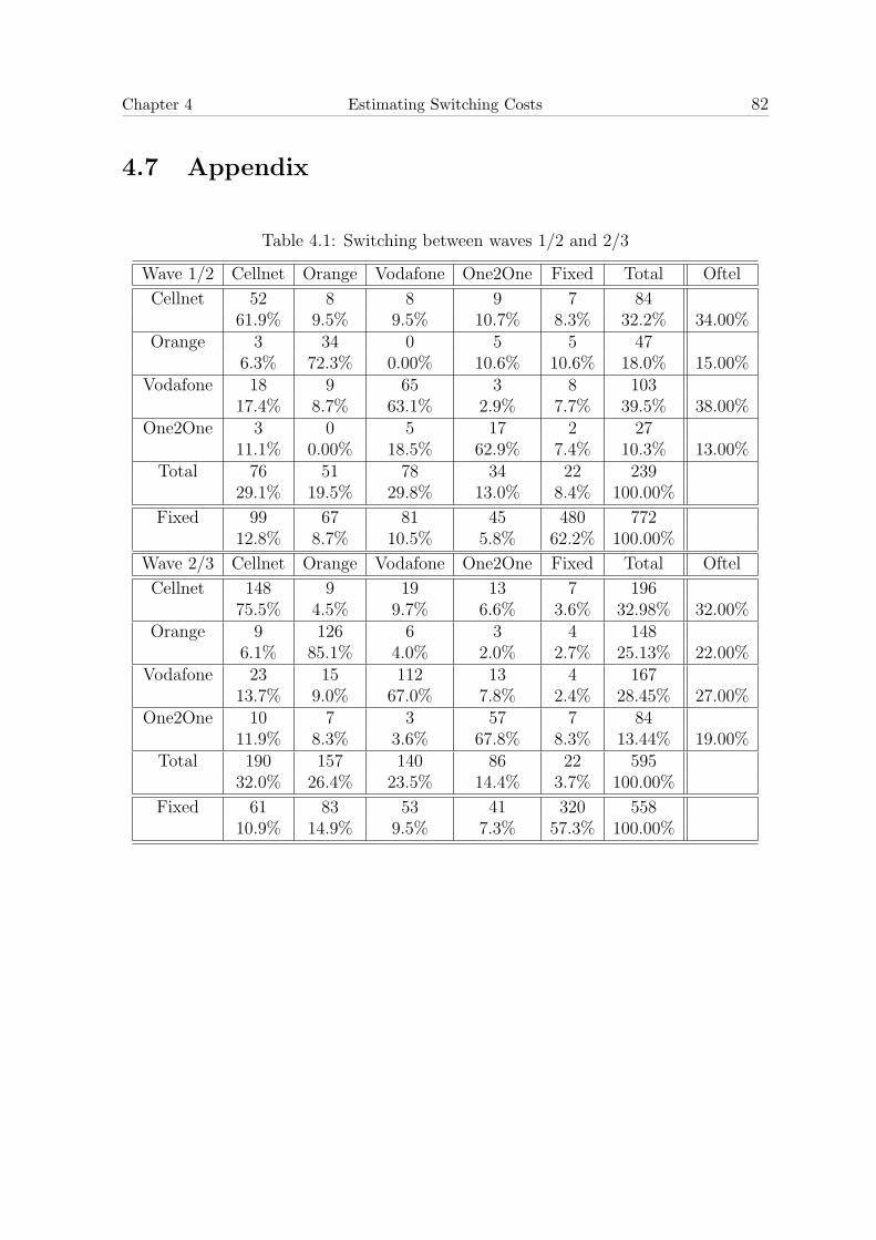
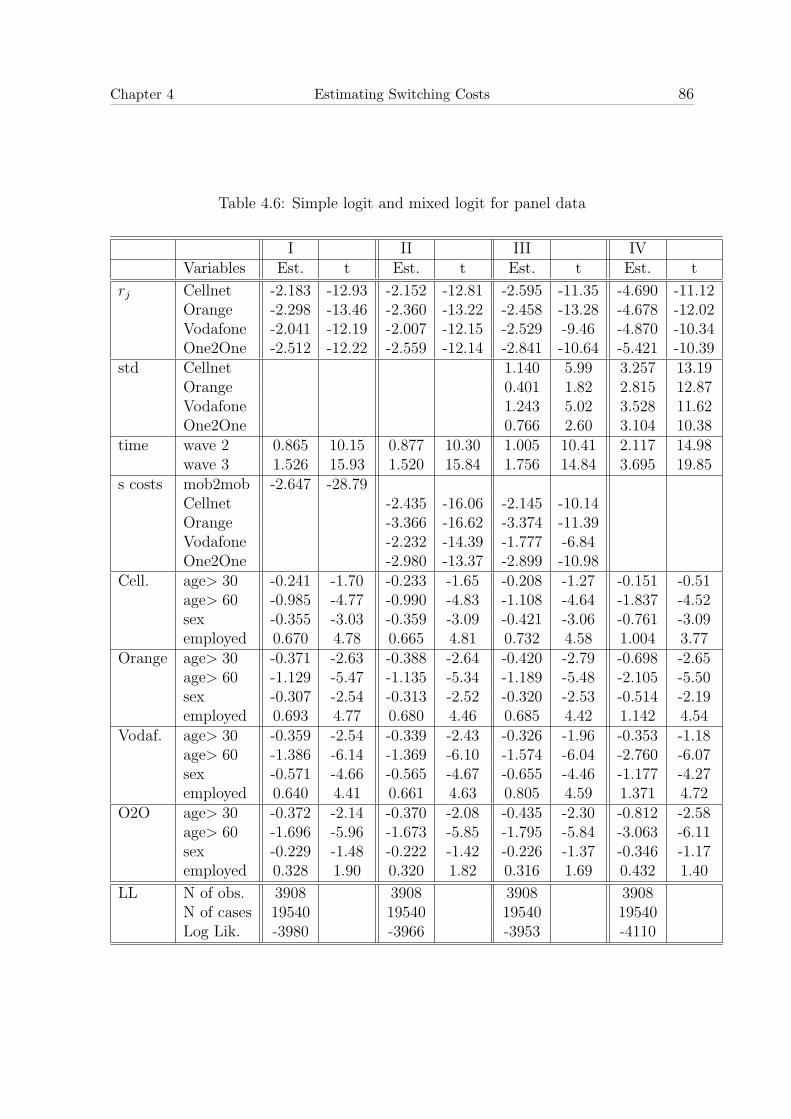
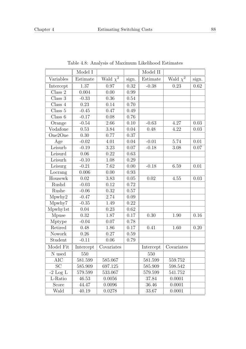
Chapter 4 presents an empirical analysis of switching costs in mobile telephony in

the UK. The presence of switching costs may have negative consequences on social

welfare because firms which have large market shares have incentives to charge higher

prices and exploit locked-in consumers rather than compete for new ones. Therefore, it

is important to provide measurements of switching costs. The empirical literature on

switching costs is scarce. This is due to the lack of appropriate detailed data sets on

individual choices. In this study, I use survey data on British households to estimate

the magnitude of switching costs in mobile telecommunications industry. I employ the

random utility framework, as developed by McFadden (1974). I estimate multinominal

and mixed logit models to identify state dependence in the choices of network opera-

Introduction 5

tors. According to mixed logit estimates for panel data there are significant negative

switching costs which vary across network operators. The choices of network opera-

tors are also explained by observable and unobservable heterogeneity of tastes. The

observable heterogeneity is represented by consumer characteristics such as: gender,

age and employment status. When multinominal logit is estimated switching costs

are overestimated due to ignorance of unobservable tastes. Thus, this study indicates

the importance of unobservable heterogeneity of tastes in the estimation of switching

costs. Both switching costs and persistent tastes of consumers lead to state-dependent

choices of network operators. Furthermore, the estimation of logistic regression indi-

cates that the probability of switching depends on consumer characteristics, such as

age, usage intensity and ways of spending leisure time. These results are consistent

with the findings in the consumer surveys conducted by the British regulator Oftel.

Chapters 3 and 4 identify and measure the magnitude of two key determinants of

competition and consumers’ choices in the mobile telephony. Apart from providing

arguments for regulatory and competition policy, it is also important to assess the

effectiveness of regulation which has been already implemented. In Chapter 5, I an-

alyze the impact of regulation on the development and competitiveness of the mobile

telecommunications industry across the European Union. In my view, the large dif-

ferences in the level of technology adoption, prices and market structure across the

EU countries are due to differences in regulatory policy and country specific charac-

teristics. I refer to earlier studies measuring the impact of regulation on the diffusion

of mobile services, such as Gruber and Verboven (2001). In a related paper, Parker

and Roller (1997) estimate the determinants of market conduct in the mobile industry

across the U.S. states. Using cross-country panel data, I estimate a reduced-form and

a structural model, and find that prices are significantly influenced by the regulatory

policy, which also explains the differences in demand for mobiles across the EU coun-

tries. In particular, the regulation implemented throughout the liberalization process

of fixed telephone lines has a negative impact on prices for mobile services. Similarly,

the implementation of number portability for mobile services has a negative impact on

prices. Moreover, I estimate country specific average industry conducts, which allow

Introduction 6

me to compare the competitiveness of mobile telephony across the European Union.

For the purpose of this study, I have created a comprehensive data set on the regulation

in telecommunications industry in the European Union.

Chapter 2

Dynamic Duopoly Competition

with Switching Costs and Network

Externalities

2.1 Introduction

A product exhibits network effects when its value increases in the number of its users.

On the other hand, switching costs arise when consumers face frictions to change

the brand they consume either due to relationship specific investments or contractual

obligations. In many industries switching costs and network effects co-exist. Take, for

example, the case of computer software and operating systems such as Windows. The

higher the number of Windows users, the more applications software will be provided

for the Windows platforms which in turn will increase the value of the operating system

inducing more people to adopt it—a typical example of indirect network effects. At

the same time, software products require investments in learning to become familiar

with their features software, which makes switching to a new set of software products

costly. Similarly, mobile telecommunications is a textbook example for direct network

effects as the higher number of subscribers imply more communication possibilities.

Chapter 2 Switching Costs and Network Externalities 8

Switching costs in mobile telephony may arise due to transaction costs, such as the cost

of changing and redistributing the phone number. Moreover, many mobile telephone

operators subsidize handsets and require consumers to sign long term contracts, which

may be costly to break.

Examples are plenty, and are presented in an illustrative manner elsewhere as in

Shapiro and Varian (1998), Katz and Shapiro (1994), Klemperer (1995) and Farrell and

Klemperer (2004). Interesting dynamic issues arising in industries with such character-

istics have attracted economists’ attention not only due to the intellectual challenges,

but also due to increasing public policy debates over the operation of these industries.

Thus, there is a large body of literature on network effects and switching costs which

arose mainly in the last two decades. In fact, the recent survey by Farrell and Klem-

perer (2004) (FK hereafter) contains 35 pages of references suggesting a mature and

saturated knowledge base.

We will follow FK in summarizing the main results of literature, and begin by

noting that both network effects and switching costs could potentially extend the con-

sumer choice problem dynamically. Current choices of consumers affect their future

consumption leading to state dependent demands. Thus, expectations of consumers on

future pricing policies and future size of sales of a firm play a key role in determining

outcomes. In certain cases, historical accidents may determine long run behavior of

a given industry. Firms face incentives inducing them to adopt “bargains-then-ripoffs

type pricing policies. That is, early on firms compete fiercely to lock-in consumers, in

order to exploit them in the future when switching costs are present, and in order to

increase the willingness to pay of future generations in case of network effects. Lock-

ing into an inferior standard, excessive private incentives for incompatibility, distorted

incentives for entry are common features of models studying such industries. In most

models, consumers do not switch between brands in equilibrium. A message FK de-

livers is the similarity of outcomes in models with network effects and models with

switching costs. For a full review of the literature, we refer the reader to FK and the


references therein.

Surprisingly, however, there is no model which studies industries where both net-

work effects and switching costs are present. Taking the risk of stating the obvious, we

would like to note that network effects have no dynamic consequences when switching

costs are nil. In such a case, it is completely optimal for consumers to be myopic,

as they can switch between brands as they please every period. In a typical dynamic

network effects model1, consumers are assumed to purchase only once, usually as soon

as they arrive to the market, and stay with their choice forever even though the net

present value of buying an alternative might become positive at a future date.

To the best of our knowledge, all existing dynamic models of network effects pre-

sume lock-in, that is sufficiently high switching costs preventing consumers from switch-

ing between brands. Hence, it is curious whether parallels drawn between the results

of models with switching costs and those with network effects are due to genuine sim-

ilarity between switching costs and network effects, or just an artifact of presumption

of lock-in in network effects models. Our goal in this paper is to attempt to identify

the consequences of network effects and switching costs both on consumer behavior

and strategies of firms when they co-exist in a meaningful way.

We adopt a very stylized model of preferences which allows consumers to switch

between brands in equilibrium. We build on the model of Klemperer (1987) by simply

appending a network benefit term to the valuation of products.2 We will consider

a simple two-period price setting model of competition between two firms which are

horizontally differentiated a la Hotelling. Only some of the consumers survive to the

next period. Those that leave the market are replaced by new consumers. Furthermore,

some consumers receive a taste shock which changes their location on the unit interval,

thus they might wish to switch the brand they buy. We assume that switching costs

are sufficiently low that at least some of these consumers will be able to change the

brand they purchase. The rest of the consumers are rigid, that is, their preferences

1See, for example, Farrell and Saloner (1986), Katz and Shapiro (1992).2When network effects vanish, the model boils down to that of Klemperer (1987).


remain as in period one as well as they have very high costs hindering any desire to

switch in the second period.3

Consumers form rational expectations of not only current network sizes but also of

future network sizes and prices. Given prices consumers are able to compute fractions

of current and future consumers buying from each firm correctly. For rational expec-

tations demands to be well-behaved, that is to avoid situations where firms can corner

the market, we assume that the marginal network benefits are sufficiently low.

We derive a subgame perfect equilibrium where firms share the market in both

periods, in the second period some of the consumers with changing preferences switch

the brands, while the rigid consumers purchase again from the same firm they shopped

in the first period. This behavior could be supported in equilibrium only for certain

parameters constellations. We derive sufficient conditions on the parameters, which

simply states that switching costs must be sufficiently low to induce switching in the

second period as well as the network effects in order to avoid tipping towards one

product in each period, and the size of the population of rigid consumers must be

sufficiently small.

The rational expectations demands we derive for each period exhibit interesting

properties. First period demands become more price sensitive with higher marginal

network benefits. In contrast, however, increasing switching costs reduce price sensi-

tivity of first period demands. Thus, in the first period switching costs and network

effects operate in completely opposite directions. In the second period, both switching

costs and network effects imply a positive shift in demand for a firm which carries over

a market share more than one half. However, the latter effect is present only when

there are switching costs. That is, in the absence of switching costs, network effects

have no dynamic consequences. The second period demands become more price sensi-

tive when marginal network benefits increase, while switching costs have no impact on

the price sensitivity.

3We keep the rigid segment in the model in order to preserve the parallels with Klemperer (1987).Alternatively, one could view our model as one with a distribution of switching costs in the population.


Second period equilibrium prices increase with the customer base of a firm carried

over from the first period. However, the subgame perfect equilibrium outcome of the

two period competition is symmetric. Thus, in both periods firms share the market

equally. Second period prices increase in the share of rigid consumers, decrease with

marginal network effects and are not affected by the switching costs.

First period prices are unambiguously reduced by higher marginal network benefits.

However, switching costs may have different effects on the equilibrium prices. We

explore how switching costs and network effects impact the equilibrium prices in the

first period by means of Monotone Comparative Statics. This allows us to uncover

the mechanisms that change equilibrium prices in response to a change in one of these

features.

First period equilibrium prices turn out to be a quadratic-convex function of the

switching costs faced by flexible consumers. Thus, for certain parameter constellations,

increasing switching costs reduce first period prices. This occurs when marginal second

period profits respond to a change in the switching costs more than first period marginal

profits. We show that this could occur when switching costs are low, in particular,

when there are no rigid consumers, there is no impact of a change in switching costs on

marginal first period profits around zero, while second period marginal profits decrease

in switching costs. Thus introducing slightly higher switching costs decrease first period

prices.

Note that some of these results are obtained in the literature in models where

switching costs and network effects are considered in isolation. Our results not only

confirm existing ones, but also provide insights when these features exist together. For

example, a policy conclusion we can draw is that whenever moderate switching costs

exist together with relatively strong network effects, the market may be sufficiently

competitive in terms of prices. Thus, a regulatory agency may refrain from costly

intervention. Furthermore, we show that the U-shaped nature of first period equilib-

rium prices can be exploited in a way to improve consumer surplus. We show that a


redistributable switching tax, even though it will always reduce aggregate welfare, may

increase aggregate consumer surplus.

In section 2, we present the model. We derive the equilibrium and discuss its

properties in section 3. Section 4 concludes.

2.2 The Model

As in Klemperer (1987), we analyze competition between two firms over two periods.

The consumer population have peculiar characteristics. For example, they value the

number of consumers purchasing a brand, they incur switching costs if they wish to

change their brand choice, and some of them have changing tastes. The model is

very stylized and builds on Klemperer (1987) by simply appending a network benefit

component to the utilities of consumers. In fact, it is equivalent to that of Klemperer

(1987) when network effects vanish. Let us begin by describing features of consumer

utilities which remain the same over the two periods. We assume that consumers have

a reservation price,4 denoted by v, that is sufficiently high so that all consumers buy

as soon as they arrive. The reservation price is the same for both products and all

consumers in any period. Furthermore, each consumer has an affinity towards one of

the brands in each period which could be due to effects of a typical consumer’s social

circle or exposure to different marketing mixes. We capture this affinity by means of a

standard Hotelling horizontal differentiation model.

Thus, we assume firms a and b are located at opposite ends of the unit interval,

that is La = 0 and Lb = 1 where Li denotes the location of firm i. Consumers are

assumed to be uniformly distributed between the two firms. If a consumer located at

x ∈ [0, 1] makes her purchase from i, she incurs a utility reduction equal to t | x−Li |,

where t measures the magnitude of this reduction, or with standard terminology unit

“transport” costs. It is important to note that we do not interpret these costs literally

4We could also refer to this term as the stand alone value, as customary in the network effectsliterature.


as transportation costs. In our model, horizontal differentiation arise due to different

reactions to marketing and hence a typical consumer may change her views over time.

Moreover, consumers derive a network benefit proportional to the number of other

consumers purchasing a given product. That is, if a product is bought by N consumers,

then each of these consumers derive a benefit equal to kN , where k measures the

magnitude of network effects. In particular, we will require the magnitude of the

network effects to be sufficiently small relative to the transportation costs in order to

avoid situations where one firm corners the market. Hence, in each period, both firms

will have positive sales.

The consumer population evolve in different ways from period one to two. Particu-

larly, only a fraction, 1−ν, of the first period consumers survive to the next period, and

those who leave the market are replaced by new unattached consumers. A second group

of mass µ, receive a taste shock, and thus, are relocated along the unit interval. This

taste shock could be interpreted as a change in a consumer’s affinity due to changes in

her social circle, as well as exposure to a different marketing mix. We assume the taste

shock to be independent of first period tastes; admittedly a rather strong assumption.5

Hence, some consumers may find a product different than what they have bought in

the first period more attractive. However, to change the brand they consume, they will

have to incur a switching cost, s, which we assume to be sufficiently small so that some

consumers switch in equilibrium. The rest of the consumer population, with a mass of

1− µ− ν, is rigid in their tastes and face much higher switching costs, sr.6 Therefore,

they continue to purchase from the firm which they bought in the first period. For

expositional ease, we refer to unattached second period consumers7 as new (n), the

group with changing preferences and low switching costs as flexible (f), and those with

5Similar modelling of changing preferences can be found in Klemperer (1987) and von Weiszacker(1984).

6Notice that even if they have changing preferences, sufficiently high switching costs would preventthem from switching.

7One could include this group to those with changing preferences, but assume that this groupincurs zero switching costs. Thus, if we allow everybody to change their preferences, we arrive at amodel with a distribution of switching costs; namely, none, moderate, and high.


high switching costs and constant tastes as rigid (r) consumers.

In summary, the net first period utility of a consumer located at x ∈ [0, 1] can be

written as

U i1(x, pi

1, Ni1) = v + kN i

1− | x − Li | t − pi1, i = {a, b}

where N iτ and pi

τ represent the expected network size and the retail price of firm i at

period τ . While the second period utility, which also is a function of their type and

first period choice, is given by

Ui|j2h (x, pi

2, Ni2) =

v + kN i2− | x − Li | t − pi

2 if i = j or j = 0, and h ∈ {n, f, r},

v + kN i2− | x − Li | t − pi

2 − s if i 6= j, j 6= 0 and h = f,

v + kN i2− | x − Li | t − pi

2 − sr if i 6= j, j 6= 0 and h = r,

Consumers choose that brand which maximizes their utility. This problem is rela-

tively easier in the second period, since consumers will learn their types, and given this

information and their expectations on the contemporary network sizes, they will select

the brand which provides them with the highest net benefit. On the other hand, the

first period choice is significantly more involved. First, consumers are uncertain about

which group they will belong to in the second period. Moreover, since their choice this

period constrains their behavior due to potential switching costs, they need to have

beliefs about future. Given prices in the first period, they need to form expectations

about current and future network sizes and future prices. We will adopt Rational Ex-

pectations (RE) as the mechanism for expectation formation. A typical consumer will

select the brand that maximizes the expected discounted sum of lifetime utilities,

U j(x, pj1, N

j1 ) = U j

1 (x, pj1, N

j1 ) + δE

[U

i|j2h (χ, pi

2, Ni2) | j, pa

1, pb1

],

where δ is the discount factor and E[· | ·] is the conditional expectations operator.

Expectations are taken over the distribution of types, and distribution of potential

second period tastes. Notice that the cumulative expected utilities depend only on the


first period observables. Consumers compute N j1 ,N j

2 and pj2 rationally. That is, N j

τ is a

demand function conditional on prices in τ , and delivers the realized network sizes for

all relevant prices for τ = 1, 2. In the first period, consumers solve the firms’ problem

in the future and anticipate second period equilibrium prices and therefore network

sizes exactly.

Firms select prices in order to maximize their discounted cumulative profits. For

simplicity we assume that firms have the same discount factor as consumers, δ. We

assume away fixed costs, and normalize marginal costs zero which is quite an innocent

assumption given the linearity of consumer utilities. We presume that firms cannot

distinguish among old locked-in and new consumers, and thus, restrict firms strategies

to nondiscriminatory, linear prices.8

2.3 The Two-Period Game

Given the preferences we have introduced, we will look for a subgame perfect equi-

librium in prices. However, we have certain ex ante restrictions on the nature of this

equilibrium. We presume that the market is covered and shared in each period which

in turn requires conditions on v and k. Furthermore, we assume some of the flexible

consumers are able to switch in equilibrium in both directions which imposes an upper

bound on s. On the other hand, the switching costs faced by the rigid types need to

be sufficiently high so that they continue buying the same brand in the second period.

Furthermore, these main features should occur for each level of market share firms

carry over from the first period. In the following, we first derive the equilibrium strate-

gies assuming that the conditions which make such outcomes possible are met, and

8We would like to note that price discrimination is potentially a powerful instrument to extractmore surplus from the locked-in consumers while competing aggressively for the new ones. If we haveallowed firms to practice price discrimination among their locked in consumers and first time buyers,they would prefer loosing their low valuation locked in customers—the ones who end up closer to theother firm in the second period—to their competitors. The intuition of this is similar to poachingbehavior studied in Fudenberg and Tirole (2000) as well as Gehrig and Stenbacka(2004). We stick withlinear pricing and no price discrimination in this paper to be comparable to the previous literature;mainly to Klemperer (1987).


then derive restrictions on the parameters such that this outcome can be supported in

equilibrium.

2.3.1 The Second Period

We start solving the two-period game by finding the second period equilibrium prices.

We first need to derive second period demand functions in order to construct the profits.

Due to switching costs, the second period choices of consumers which remain in the

market depend on their first period choices, therefore we need to find the demands

from each consumer group. Let us first consider the new unattached consumers who

are distributed uniformly along the unit interval with mass ν. This group simply

compares the utilities from product a and b, and select the brand which provides them

the highest net benefit. Thus, finding the indifferent consumer is sufficient to identify

the demand faced by firms from this group of consumers. Formally, let da|02 denote

this location, then it must satisfy Ua|02n (d

a|02 , pa

2, Na2 ) = U

b|02n (1 − d

a|02 , pb

2, 1 − Na2 ) where

pi2 and N i

2 are the second period price and expected network size of firm i respectively.

Notice due to the fact that consumers are uniformly distributed, da|02 also is equal to

the fraction of new consumers buying from firm a. Solving this equation yields,

da|02 =

1

2+

k

2t[2Na

2 − 1] +1

2t[pb

2 − pa2], (2.1)

and since we assume that the market is covered db|02 = 1 − d

a|02 .

The group of flexible consumers, which has a mass of µ, evaluate each product anew

as they are now placed at a different point along the unit interval. For example, one

consumer who was closest to firm a in period one, could very well be closer to firm b in

period 2. Therefore, who they have bought from in the first period has a crucial impact

on their second period choice. Let us first consider those who have bought from a in the

first period. Identifying the demands of this group of consumers is once again equivalent

to finding the indifferent consumer with one difference. Even though firm 2 announces


a retail price of pb2, consumers face pb

2 +s when they consider buying from b. Recall our

prevailing assumption that switching costs, s, are sufficiently low that some will prefer

switching to firm b. Let us denote the fraction of consumers from this group which

prefer firm a by da|a2 . Then, it must satisfy U

a|a2f (d

a|a2 , pa

2, Na2 ) = U

b|a2f (1−d

a|a2 , pb

2, 1−Na2 ),

and is given by

da|a2 =

1

2+

k

2t[2Na

2 − 1] +1

2t[pb

2 + s − pa2]. (2.2)

The fraction of consumers who has bought a in the first period, but prefers b in

the second period is simply db|a2 = 1 − d

a|a2 . Applying similar arguments, the frac-

tion of flexible consumers who have purchased from b and switches to a, da|b2 , solves

Ua|b2f (d

b|a2 , pa

2, Na2 ) = U

b|b2f (1 − d

a|b2 , pb

2, 1 − Na2 ), and is given by

da|b2 =

1

2+

k

2t[2Na

2 − 1] +1

2t[pb

2 − pa2 − s]. (2.3)

Likewise, the fraction of consumers who remain loyal to b is db|b2 = 1−d

a|b2 . Notice that

these consumers perceive firm a’s price as pa2 + s.

Finally, the fraction of consumers with unchanged preferences (1−ν−µ) will choose

in the second period exactly the same brand as before, since their switching cost sr is

assumed to be sufficiently high.

Therefore, the total second period demand faced by firm i ∈ {a, b} in period 2 is

given by

di2 = µ[d

i|a2 Na

1 + di|b2 N b

1 ] + (1 − µ − ν)N i1 + νd

i|02 , i = {a, b}. (2.4)

Rational expectations about the network sizes imply N a2 = da

2 and N b2 = 1 − Na

2 =

1 − da2 = db

2. Let

α =sµ + t(1 − µ − ν)

2(t − kµ − kν)

and

β =µ + ν

2(t − kµ − kν).


Solving (2.4) with imposing the rational expectations restrictions yields

da2 =

1

2+ β(pb

2 − pa2) + α[2Na

1 − 1], (2.5)

and db2 = 1−da

2. For each firm to face downward sloping demand curves, t−kµ−kν > 0

must hold; that is, the network benefits must be relatively small compared to the

transportation costs or the share of rigid consumers must be relatively high.

It is easy to verify that whenever t − kµ − kν > 0

∂α

∂s=

µ

2(t − kµ − kν)> 0,

∂β

∂s= 0,

∂α

∂k=

(sµ + t(1 − µ − ν))(µ + ν)

2(t − kµ − kν)2= 2αβ > 0,

and

∂β

∂k=

(µ + ν)2

2(t − kµ − kν)2= 2β2 > 0.

Thus, a close inspection of (2.5) suggests that, the second period demand of a firm

with a user base larger than one half shifts outward, while the demand of the other

firm contracts when switching costs increase. However, the price responsiveness of the

demand is not affected by the same change which is an artifact of our two period model.

Since there is no future, neither the new consumers nor the flexible ones need to worry

about low current prices implying high ones in the future and vice versa.

Similarly, a slight increase in k not only shifts the demand of the firm with a higher

user base outward, but also makes the demands more sensitive to price differentials.

The price effect is due to rational expectations; i.e., consumers observing a price dif-

ferential expect the demand of the lower price firm to increase both due to an increase

in utility via price directly and via the network benefits indirectly. The upward shift

in demand however occurs only when coupled with switching costs. When s = 0 and


ν + µ = 1, that is when there are no switching costs and no rigid consumers, the

network effects only have an impact via price sensitivities.

It is exactly this point which has not received much attention in the literature.

The similarities between results obtained in models with switching costs and in models

with network effects arise due to the outward shift of the demand when consumers are

locked-in. But what locks consumers in is not the network effects, it is the switching

costs which are usually assumed to be very high that no one switches.

Given that the fixed and marginal costs are normalized to zero, the second period

profit functions of the firms are simply their revenues and given by Πa2 = pa

2da2 and

Πb2 = pb

2db2. And due to the linearity of demands, the profit functions are concave in

the own price of each firm.9 Thus, first order conditions(FOCs) describe a candidate

Nash equilibrium with prices given by

pi2 =

1

2β+

α

3β[2N i

1 − 1] (2.6)

=t

ν + µ− k +

1

3

(s µ + t(1 − ν − µ))(2 N1

i − 1)

ν + µ, i = {a, b}.

However, note that we have imposed certain behavioral assumptions on the demand

side when we derived rational expectations demands. These behavioral assumptions

translate to constraints which firms should take into account when formulating their

best responses. Namely, we require some consumers to switch brands in the second

period which is only possible when 0 < da|b2 ≤ d

a|a2 < 1. If this condition holds, then

0 < da|02 < 1, since d

a|b2 ≤ d

a|02 ≤ d

a|a2 . Observe that both d

a|a2 and d

a|b2 will be functions

of N i1 in equilibrium, therefore these restrictions should hold for every possible value of

N i1, namely 0 ≤ N i

1 ≤ 1. This is necessary, since, in the first period, firms would foresee

the equilibrium in the second period. By restricting our attention to cases where the

postulated behavior occurs for each N i1, we avoid situations where second period profit

functions become non-differentiable for certain strategies that might arise in the first

9Notice that β ≥ 0.


period.

Furthermore, as µ + ν → 0, firms place a higher weight on revenues from the rigid

consumers, and since these consumers face very high switching costs, each firm will find

it most profitable to exploit this segment to the fullest extent. Namely, they might

select their prices in order to drive the net surplus of the marginal rigid consumer to

zero, which in turn might drive their demand from new and flexible consumers to zero.

In fact, such a strategy may be profitable for any value of µ+ν when v is large enough.

Remember also that we have assumed v to be sufficiently large that all consumers buy

for reasonable ranges of prices. Even though we do not explicitly derive the necessary

conditions, we assume that v is sufficiently large to induce all consumers to participate,

while it is sufficiently small that neither firm finds it optimal to just serve the rigid

consumers for all 0 ≤ N i1 ≤ 1 and all reasonable prices of the other firm.

Let

P =

{

µ + ν ∈

[2

5, 1

]

, k ∈

[

0, kmax

]

, s ∈

[

0, smax

]}

where

smax = t −t(1 − ν)(1 − kβ)

tβ + (2µ + ν)(1 − kβ),

and

kmax =2

3t.

At the candidate equilibrium prices, the type of behavior we have postulated, i.e. new

consumers buy from both firms, some flexible consumers switch to the other brand,

and rigid ones stick to their first period choice, is realized if parameters belong to P .

Lemma 1 A sufficient condition for the second period prices given in (2.6) to consti-

tute a Nash equilibrium is (µ + ν, k, s) ∈ P. At these prices, the equilibrium demands

are

di2 =

1

2+

1

3α(2N i

1 − 1) (2.7)


and the equilibrium profits are

Πi2(N

i1) =

1

36β[3 + 2α(2N i

1 − 1)]2 (2.8)

where i = {a, b}.

Proof. See Appendix.10

The second period equilibrium prices have a few interesting properties. First observe

that, whenever k < kmax, t−kµ−kν > 0, thus β is positive and demands are downward

sloping. Moreover, since α is also positive, the demand function of a firm carrying over

a market share that is larger than one half from the first period shifts outward enabling

this firm to charge a higher price. Furthermore, the second period profits are increasing

in the first period customer base which makes lock-in valuable. This would give both

firms incentives to compete more fiercely in the first period.

Both second period equilibrium prices and profits increase in switching costs when

a firm has a customer base, N i1, that is larger than one half. Thus, a firm which

dominates in terms of market shares in the first period would benefit from an increase

in the switching costs. On the other hand, an increase in the network effects, k, decrease

both the price and profit of a firm which carries over more than half of the first period

consumers to the second period. Hence, switching costs and network effects are forces

which act in completely opposite directions in equilibrium in the second period.

If the firms carry over a market share that is closed to one half from the first period

and µ + ν → 1, then the second period equilibrium prices could well fall below t, the

price which would have prevailed in the absence of switching costs and network effects.

Consequently, the presence of network effects might make the second period fiercely

competitive as well.

10We would like to emphasize once again that the restrictions defining P are only sufficient but notnecessary to induce the postulated behavior. Thus, the equilibrium prices are valid for a larger set ofparameters.


2.3.2 The First Period

Consumers face a much more complicated task in decision making in the first period.

They need to evaluate a stream of benefits for two periods for each product in order

to select one. Consumers do not know their type initially, thus they need to figure out

their second period actions conditional on first period choices as well as the realizations

of their type. With probability ν, they will leave the market in which case they receive

no benefits, while with probability 1 − µ − ν, they will be rigid and will buy the same

brand as in the first period. They will belong to the group of flexible consumers, i.e.

will be redistributed along the unit interval, with probability µ. Therefore, they will

switch to the other brand with some probability whichever brand they buy in the first

period. For example, if they are considering the second period benefit conditional on

having bought brand a in the first period, they will know that they will switch to brand

b if their new location along the unit interval is larger than da|a2 and remain with brand

a otherwise. Formally, their expected benefit will be

EUa =

∫ da|a2

0

Ua|a2f (χ, pa

2, Na2 )dχ +

∫ 1

da|a

Ub|a2f (χ, pb

2, Nb2)dχ.

Similarly, the expected benefit of a flexible consumer conditional on buying brand b in

the first period can be written as

EU b =

∫ da|b2

0

Ua|b2f (χ, pa

2, Na2 )dχ +

∫ 1

da|b

Ub|b2f (χ, pb

2, Nb2)dχ.

In doing these complicated calculations, we assume that consumers rationally infer

next period prices (pa2, p

b2), next period network sizes (N a

2 , N b2) and critical values de-

termining whether they switch or not, (da|a2 , d

a|b2 ). Observe that each of these quantities

in equilibrium turns out to be a function of first period customer base of each brand,

and thus, first period prices. Therefore, given first period prices, rational consumers

should be able to compute first period demands which in turn determine second period


equilibrium prices, network sizes, and critical values.

Hence, in the first period, a rational consumer chooses that brand which delivers

highest lifetime utility, that is they compare

Ua(x, pa1, N

a1 ) = [v − pa

1 − tx + kNa1 ] + δ

[

µEUa + (1 − µ − ν)[v − pa

2 − tx + kNa2

]]

and

U b(x, pb1, N

b1) = [r − pb

1 − t(1 − x) + kN b1 ]

+δ

[

µEU b + (1 − µ − ν)[r − pb

2 − t(1 − x) + kN b2

]]

.

Computing the difference yields

Ua(x, pa1, N

a1 ) − U b(x, pb

1, Nb1) = pb

1 − pa1 + (t − k + 2kNa

1 − 2tx)

+δsµ

t

(k(2Na

2 − 1) + pb2 − pa

2

)(2.9)

+δ(1 − µ − ν)(pb

2 − pa2 + (t − k + 2kNa

2 − 2tx)),

where we have used N b1 = 1 − Na

1 and N b2 = 1 − Na

2 . Observe that the right hand side

of (2.9) is decreasing in x, the distance from brand a. Thus, if there is a consumer

indifferent between the brands, all those consumers to the left will purchase brand a

and to the right will buy brand b.

The demands faced by firms, once again, can be identified by finding the location of

the indifferent consumer in the first period. Let da1 denote this location then it solves

Ua(da1, p

a1, N

a1 ) − U b(da

1, pb1, N

b1) = 0. (2.10)

Rational expectations on first period network sizes require da1 = Na

1 = 1−N b1 = 1−db

1.

Imposing this condition as well as substituting second period prices from (2.6), second

period rational expectations network sizes from (2.7), we solve (2.10) for the first period


demands yielding

di1 =

1

2+

pj1 − pi

1

γ, i ∈ {a, b} and j 6= i, (2.11)

where

γ = 2(t − k) + 2tδ(1 − µ − ν) +4

3

αδ(sµ + t(1 − µ + ν))(1 − kβ)

tβ.

Whenever k ≤ kmax, we have t− k > 0 and 1− kβ > 0, implying γ > 0, therefore first

period demands are downward sloping.11

Switching costs and network effects have their impact on the first period demands

through γ. A brief inspection reveals that

∂γ

∂k= −2 −

8δα2

3< 0,

and

∂γ

∂s=

8δµα(1 − kβ)

3tβ> 0.

That is, the first period demand becomes more sensitive to prices with an increase in

network effects, while they become less price sensitive with an increase in switching

costs. The latter is due to the fact that, rational consumers forecast a larger price

for the firm which carries over a larger customer base to the second period—the lower

priced firm in the first period. Hence, consumers do not easily buy in to initial price

cuts. On the other hand, a lower price in the first period implies a larger group of

consumers who would be “locked-in” in the second period implying a larger network

benefit. A lower price in the first period allows consumers to coordinate on one firm not

only in the first period but also in the second period. The difference between switching

costs and network effects are starker in the first period; they are demand side forces in

completely opposite directions.

11We would like to note that when k = 0, γ reduces to y introduced in Klemperer (1987) pp. 148.


The cumulative profit functions of the firms are Πa = pa1d

a1 + δΠa

2(da1) and Πb =

pb1d

b1 + δΠb

2(db1), where Πa

2 and Πb2 are the second period equilibrium profits given in

(2.8). These profit functions are concave in own prices whenever 4δα2 < 9γβ. We show

in the appendix that when we restrict our attention to parameters in P , this condition

indeed is satisfied. Hence solving the FOCs yields symmetric first period candidate

equilibrium prices given by

pa1 = pb

1 =1

2γ −

2δα

3β. (2.12)

At these prices the profits of the firms are equal and given by

Πi =γ

4+

δ

4β−

δα

3β, i = {a, b}, (2.13)

which we show, in the appendix, to be non-negative when (µ + ν, k, s) ∈ P .

Proposition 1 A sufficient condition for the prices given in (2.12) to constitute a

Nash equilibrium in the first period is {µ + ν, k, s)} ∈ P. The equilibrium first period

demands turn out to be

da1 = db

1 =1

2. (2.14)

Given the first period customer bases, the second period equilibrium prices are also

symmetric and given by

pa2 = pb

2 =t

µ + ν− k (2.15)

while the equilibrium demands in the second period also turn out be

da2 = db

2 =1

2. (2.16)

Proof. See appendix.

The second period equilibrium prices12 are always positive, while the first period

12Note once again that we only provide sufficient conditions in proposition 1, and the equilibriumis valid for a larger set of parameters.


prices could be negative. 13 The first period equilibrium prices are quadratic convex

in s—a feature we explore further when µ + ν → 1 below. It is important to note

that the quadratic convex nature of equilibrium prices implies that for some parameter

constellations, increasing the switching cost slightly may lead to a decrease in first

period prices. This is particularly interesting since we have previously shown that

increasing the switching costs reduces demand elasticities in the first period. However,

it also increases the value of carrying over a larger user base to the second period. We

analyze the relative importance of these effects in subsection 2.3.3.

Klemperer (1987) recognizes that first period prices may be lower than those in

a market without switching costs. However, he does not acknowledge the U-shaped

nature of of first period prices in switching costs which may have further policy impli-

cations. We present one such implication in subsection 2.3.5.

On the other hand, both first and second period prices decrease in the marginal

network benefits, k.14 Therefore, when there are network effects, anticompetitive con-

cerns in markets with switching costs may be reduced. In fact, the higher the network

effects the lower the prices, and there may be cases where prices fall below those in

a market without rigid consumers, network effects and switching costs. That is, any

worry policy makers might have concerning high prices due to switching costs may not

be well founded in the presence of sufficiently strong network effects.

Let pskτ be the equilibrium prices in the presence of both switching costs and net-

work effects, pkτ be the equilibrium price when only network effects exist, ps

τ be the

equilibrium price with just switching costs and pτ be the equilibrium price without

switching costs and network effects in period τ . It is easy to verify that p2 = t/(µ + ν)

and p1 = t(1 + δ(1 − µ − ν)/3). Observe that as µ + ν → 1, both p1 and p2 approach

t, the price that would have prevailed in a static standard Hotelling model. In the

following proposition, we summarize relationships of these prices both in the first and

13One likely configuration where first period prices can be negative occurs when s → smax, k →kmax, δ → 1, µ + ν → 1 and µ > 1/2.

14First period prices are decreasing in k, since γ is decreasing in k, while α/β is constant in k.


second period.

Proposition 2 (Price Orders)

1. The second period equilibrium prices can be ordered in two ways:

• Low network benefits: ps2 > psk

2 > p2 > pk2

• High network benefits: ps2 ≥ p2 > psk

2 > pk2,

2. The first period equilibrium prices must fulfill two conditions:

• ps1 > psk

1 and p1 > pk1

Notice the indeterminacy of first period price rankings. As we have noted above,

first period prices could fall below marginal cost—zero, in our model—for certain pa-

rameter constellations. In the next subsection, we investigate the incentives of firms

in setting their prices in the first period, and try to uncover the mechanisms through

which switching costs and network effects shape the first period equilibrium. The clear

message, however, is that the presence of network effects reduce prices in both periods.

2.3.3 The Monotone Comparative Statics

In this subsection, we explore further the impact of switching costs and network effects

on first period prices. We employ monotone comparative statics (MCS) to uncover the

mechanisms both these features affect the incentives of the firms.15 The MCS allow

us to separate the impact of switching costs and network benefits on the equilibrium

prices into first and second period effects. In the arguments below we maintain the

assumption that the parameters are in the set where the equilibrium we have derived

in Proposition 1 exists.

15In doing so we follow Vives (1999), pp.34-39.


The derivative of the best response function of firm a, R(pb1, s, k) with respect to

switching costs can be written as16

∂

∂sR(pb

1, s, k) = −

∂2

∂s∂pa1

Πa(R(pb1, s, k), pb

1, s, k)

∂2

∂pa1

2 Πa(R(pb1, s, k), pb

1, s, k).

The denominator is negative because the profits are concave in pa1. Thus, the sign of

the left hand side depends on the sign of the numerator, which is determined by a few

non-zero partial derivatives and given by17

∂2Πa

∂s∂pa1

= pa1

∂2da1

∂s∂pa1

+δpa2

[(∂da

2

∂pb2

∂pb2

∂da1

+∂da

2

∂da1

)∂2da

1

∂s∂pa1

+

(∂da

2

∂pb2

∂2pb2

∂s∂da1

+∂2da

2

∂s∂da1

)∂da

1

∂pa1

]

(2.17)

When we evaluate (2.17) at the first period equilibrium prices, we obtain the direc-

tion of change in the best response function of firm a in the first period due to a change

in s around the equilibrium. After substituting the expressions for partial derivatives

and equilibrium prices, we get

∂2Πa

∂s∂pa1

=3γβ − 4αδ

6β

8δµα(1 − kβ)

3tγ2β︸︷︷︸

+/−

+δ1

2β

[

β

(

−2α

3β

)8δµα(1 − kβ)

3tγ2β︸︷︷︸

−

+ 2α8δµα(1 − kβ)

3tγ2β︸︷︷︸

+

(2.18)

+ β

(

−2µ

3(µ + ν)

)(

−1

γ

)

︸︷︷︸

+

+µ

t − µk − νk

(

−1

γ

)

︸︷︷︸

−

]

,

which after simplifications yields

∂2Πa

∂pa1∂s

=2δ µ

3γtβ

(

2 α (1 − k β) −t β

ν + µ

)

. (2.19)

16We will only present the results here; see appendix for their derivation. Similar arguments applyfor the best response function of firm b due to symmetry.

17In writing (2.17), we suppressed arguments of da1

= da1(pa

1, pb

1, s, k), pb

2= pb

2(da

1(pa

1, pb

1, s, k), s, k),

and da2

= da2(pa

2(da

1(pa

1, pb

1, s, k), s, k), pb

2(da

1(pa

1, pb

1, s, k), s, k), da

1(pa

1, pb

1, s, k), s, k).


All derivatives in (2.17) have definite signs except the first period effect, which de-

pends on the sign of first period prices. Switching costs affect second period marginal

profits through several different channels, however overall effect is ambiguous.18 When

first period prices are positive, marginal first period profits are increasing in the switch-

ing costs. This is due to the increase in γ, which in turn reduces first period demand

elasticity. The reduction in the first period demand elasticity also impact second period

incentives, first, through a negative indirect effect of the second period price of firm b,

pb2, on firm a’s second period demand, da

2 (2nd term in (2.17)); and second, through a

positive direct effect of the first period demand, da1, on the second period demand (3rd

term in (2.17)). The overall contribution of these three effects on the incentives of firm

a is positive yielding incentives to increase first period price, irrespective of the sign of

the first period equilibrium prices.

The fourth term in (2.17) results from the decrease in the responsiveness of second

period price of firm b, pb2, to the first period demand, da

1, due to an increase in switching

costs. When the first period price, pa1, increases, the first period demand, da

1, falls,

which encourages firm b to raise its second period price, pb2, and therefore the second

period demand, da2, and profits increase. When switching costs grow in magnitude,

the increase in firm b’s price is more, leading to incentives for firm a to increase first

period prices. The fifth term is due to a positive change in the responsiveness of the

second period demand, da2, to the first period demand when switching costs increase.

An increase in the first period price pa1 decreases the first period demand da

1, which

decreases the second period demand da2 and the profits. When switching costs rise,

the second period demand decreases more implying a negative impact on profits which

leads to an incentive to decrease first period prices. It is straightforward to show that

these two effects combined have a negative sign.

The overall direction of the movement of the best response function of firm a is

ambiguous. However, notice that the term in parenthesis in (2.19) is linearly increasing

18All the arguments below are based on the sign of partial derivatives given in (2.18), however theyare followed best referring to equation (2.17).


in s.19 Thus, if the right hand side of (2.17) is positive at s = 0, it is positive for all s.

Otherwise, best response function of firm a shifts downwards around the equilibrium

for small s, implying lower equilibrium prices with a slightly higher s.

A similar analysis can be performed for network benefits. The change in the mar-

ginal profits due to a change in marginal network benefits, k, is induced through three

non-zero partial derivatives

∂2Πa

∂k∂pa1

= pa1

∂2da1

∂k∂pa1

+ δpa2

[∂da

2

∂pb2

∂pb2

∂da1

+∂da

2

∂da1

]∂2da

1

∂k∂pa1

, (2.20)

after the substituting the expressions for partial derivatives and equilibrium prices we

obtain

∂2Πa

∂k∂pa1

=3γβ − 4αδ

6β

(

−6 + 8δα2

3γ2

)

︸︷︷︸

+/−

+δ1

2β

[

β

(

−2α

3β

)(

−6 + 8δα2

3γ2

)

︸︷︷︸

+

+ 2α

(

−6 + 8δα2

3γ2

)

︸︷︷︸

−

]

(2.21)

= −3 + 4δα2

3γ< 0. (2.22)

Apart from the first period term, once again the effects of an increase in network

benefits have well determined signs. The overall effect is unambiguously negative,

implying that best response function of firm a shifts down around the equilibrium.

Since firm b’s reaction function moves also downward, equilibrium is obtained at lower

prices when network effects increase.

In contrast to the switching costs, higher network benefits result in a more elastic

demand in the first period for positive prices. And, the impact of increasing network

effects on the cumulative profits only operate through this increase in first period

demand elasticity as can be seen in (2.20). The second period effects go through two

19This is due to the fact that α is linearly increasing in s.


channels, first a negative indirect effect of firm b’s second period price, pb2, on firm a’s

second period demand, da2, and second, through a direct positive impact of the first

period demand of firm a on the second period demand.

In summmary, the MCS we present in (2.18) and (2.21) not only allow us to dis-

entangle the first and second period effects of changes in switching costs and network

effects on pricing incentives of the firms in the first period, but also to identify the

channels which these changes affect incentives.

2.3.4 The Case without Rigid Consumers

A few of the results we have presented in the previous subsection become sharper when

we consider the case without rigid consumers, i.e., µ + ν → 1. This simply assumes

that every consumer, which survives from period one to two, could potentially switch,

and firms as well as consumers are all aware of this possibility. A brief inspection

of (2.12), suggest that second period prices decrease, however, the effects in the first

period prices is not immediately seen as decreasing the size of the rigid consumers

negatively impact second period profits and could reduce the first period incentives to

lock customers in. Nevertheless, if we keep µ constant and let ρ = µ + ν, i.e., replace

rigid consumers with new unattached ones, it is possible to show that

∂pa1

∂ρ= −

1

3

(2 s µ (t − k ρ)2 (s µ + t) + (s µ k − t (t − k))2 ρ2

)δ

ρ2t (t − k ρ)2 < 0,

thus also first period prices decrease.

Next, we investigate the effect of changes in switching costs faced by flexible con-

sumers and network effects when µ + ν → 1. Substituting µ = 1 − ν in (2.17), after

simplifications, yields

∂2Πa

∂s∂pa1

=δ(1 − ν)[s(1 − ν)(2t − 3k) − t(t − k)]

δ(1 − ν)2s2(2t − 3k) + 3t(t − k)2(2.23)


The denominator is always positive when k < kmax. Hence, the sign of this expression

depends on the numerator, which is positive for s > t(t−k)(1−ν)(2t−3k)

and negative otherwise.

More importantly, when s = 0, a slight increase in switching costs shift both best

response functions downwards leading to lower first period equilibrium prices. Thus,

when switching costs are sufficiently low, the incentives to exploit locked-in consumers

in the second period dominates and first period competition is fiercer.

In particular, consider the case when switching costs are zero, which implies first

period equilibrium prices of pi1 = t − k. After substitution of µ = 1 − ν and s = 0 in

(2.18), one can show that

∂2Πa

∂s∂pa1

∣∣∣∣∣s=0,µ=1−ν

= 0 + δ(t − k)

[

0 + 0 +1 − ν

6(t − k)2−

1 − ν

2(t − k)2

]

= −δ(1 − ν)

3(t − k).

Clearly the decrease in equilibrium prices is due to the impact of a small increase in

switching costs on future profits, since the first period effect is identically zero. A

similar result can be found in Doganoglu (2005) where it is shown in a fully dynamic

setup that small switching costs might lead to lower prices in steady state compared

to no switching costs.

2.3.5 Switching Taxes: A Policy Suggestion

In this subsection, we present a rather interesting policy implication of our results.

The fact that by making switching costly between firms, first period equilibrium prices

may be reduced suggests that there is a possibility of increasing first period consumer

benefits. A feature of our model which limits this increase is the fact that market size

is constant. That is, we assume that all the consumers buy anyways, therefore the

reduction in prices do not lead to an increase in the size of the consuming population.

The effects of switching costs on market participation remains an interesting issue to

explore, however it is beyond the scope of the current paper. Still, we are able to argue

below that even though introduction of a switching tax reduces aggregate welfare,


consumer surplus can be increased in detriment to firms’ profits.

After lengthy but straightforward computations, aggregate welfare, that is the

equally weighted sum of the consumer surplus and profits, turns out to be

W = (1 + δ)(r −t

4) + (1 + δ)

k

2− δsµ(

1

2−

s

2t) −

δµs2

4t. (2.24)

The first term represents the welfare in a market without switching costs and network

effects over two periods. The second term accounts for the aggregate network benefits,

as every consumer has access to a network of size one half in both periods. The third

term corresponds to the losses which arise in the second period when some flexible

consumers decide to incur the switching costs and change the firm they buy from. The

fourth term, on the other hand, is due to the inefficient allocation of flexible consumers

to the firms in the second period. Notice that some flexible consumers located to the

right of the midpoint between the firms continue to buy from firm 1 in the second

period instead of patronizing firm 2 which is closer to their location. This introduces

a welfare loss as the cost of extra distance travelled by these consumers.

If a policy maker were to institute a switching tax, some of the losses in the second

period could be avoided by refunding the tax revenue to consumers. That is, the

third term in (2.24) will vanish if s were to be interpreted as a redistributable tax.

This interpretation is more sensible when there are no rigid consumers, i.e. when

µ + ν → 1—a case we focus on below. Nevertheless, such a tax would still reduce

aggregate welfare due to inefficient allocation of consumers among the firms in the

second period, since the fourth term in (2.24) will not vanish. However, incurring this

cost may yield a significant shift of surplus from the firms to the consumers via the

decrease in the first period prices. Whenever µ + ν → 1, the first period prices can be

simplified to

p∗1 = t − k −2

3tδµs(t − µs) −

δµ2s2k

t(t − k). (2.25)

Notice that the last two terms are negative whenever the equilibrium we describe in


proposition 1 exists, hence, introducing a switching tax, s, will reduce prices in the

first period.

Consider an industry without switching costs and no rigid consumers. Introducing

a redistributable switching tax, s, will increase consumer surplus in the first period by

an amount equal to the last two terms of (2.25), while reducing it in the second period

by an amount equal to the fourth term of (2.24), hence the net change in consumer

surplus is given by

∆CS =2

3tδµs(t − µs) +

δµ2s2k

t(t − k)−

δµs2

4t,

which is easily shown to be quadratic concave function of s, with ∂∆CS/∂s∣∣s=0

> 0.

Therefore, the change in consumer surplus is positive for positive switching tax levels.

As we mentioned above, such a policy may increase consumer surplus, nonetheless

reduce profits even more that the aggregate welfare will go down. A policy maker

whose objective is biased towards consumer benefits, i.e. one which places a much

lower weight to profits, would find such a policy attractive however. Doganoglu (2005)

presents a similar case in favor of switching taxes in a fully dynamic model based on

welfare comparisons in the steady state.

2.4 Conclusion

We have analyzed the two-period model of duopolistic competition with switching

costs and network effects, built on the model of Klemperer (1987). We have shown

that switching costs and network effects are forces in opposite directions early on. That

is, consumer would like to be part of a network which would be large in the future. But

firms with large user bases are able to sustain high prices in the presence of switching

costs, thus reducing their attractiveness for consumers early on. The clear signs of these

phenomena can be exemplified in our first period demands, which becomes more(less)

price sensitive with an increase in marginal network benefits (switching costs). When


there are no switching costs, the size of a network does not play an important dynamic

role, as can be seen in the second period demands we have derived. Network effects

increase price sensitivity of consumers when expectations are rationally formed, since

in this case a price decrease not only has a direct positive impact on the utility of a

marginal customer, but also an indirect effect through the network benefits.

Subgame perfect(SP) equilibrium prices in both tend to be lower as network effects

increase. In both periods, this is due to increased price elasticity of demands faced by

firms. The effects of switching costs, on the other hand, on the equilibrium outcomes

are less clear cut. In the second period, the switching costs faced by flexible consumers

tend to increase the price charged by a firm which carries over an installed base larger

than one half. However, in the SP equilibrium of the whole game, switching costs have

no effect. Nevertheless, the second period on the SP equilibrium prices increase with

an increase in the size of the population of rigid consumers.

The effects of switching costs on the first period equilibrium prices is ambiguous.

Even though the firms face demands with a lower price elasticity when switching costs

increase, they also face a more profitable second period when they are able lock in

more than half of the first period consumers. While the former effect leads to incen-

tives to increase prices, the latter encourages firms to reduce their prices. Hence, the

equilibrium is attained when these opposing incentives are balanced.

However, there is no telling ex-ante where this balancing would occur. Thus our

first period prices could be lower than those in a market without network effects and

switching costs. We show that the first period prices are quadratic-convex functions of

the level of switching costs, therefore for certain parameter values increasing switching

costs may reduce equilibrium prices. We can see this clearly in our example without

rigid consumers, where around zero, increasing switching costs have no impact on

marginal first period profits while it reduces second period profits, leading to lower

equilibrium prices.

This point is very important to note, as the common message in the literature


studying fully dynamic models is that switching costs unambiguously increase steady

state prices. A common assumption shared by all the fully dynamic models is that

switching costs are sufficiently high that consumers do not expect to switch, and in

equilibrium there is no switching. However, it is not obvious whether this would be

the case for small switching costs as our model in this paper suggests. Essentially, one

would expect that in a fully dynamic model, firms would be in a situation much like

the first period, but at the same time have some installed bases. Thus in a steady

state, we expect the prices to inherit the same U-shape as we have derived in this

paper. In a related model, Doganoglu (2005) shows that in fact for small switching

costs steady state prices may be below those in a market without switching costs. We

have shown that this property may be exploited to increase aggregate consumer surplus

by introducing a switching tax.

Naturally, there are a few directions in which one could extend this paper. We

think that a fully dynamic analysis is warranted. A more interesting issue is related

to the market size. In this model, the total demand is completely inelastic, that is all

consumers buy no matter what. However, both network effects and switching costs

are likely to have effects on the participation incentives of the marginal consumer. A

thorough welfare analysis could only be conducted, when these incentives are taken

into account.


2.5 Appendix

Proof of Lemma 1

We have imposed certain behavioral assumption on the demand side when we derived

rational expectations demands in the second period. Namely, market is covered, both

firms make positive sales to all the consumer types, and some flexible customers of each

firm find it better to switch to the other brand. Switching in both directions occur, for

each Na1 ∈ [0, 1], only when

0 < da|b2 ≤ d

a|a2 < 1,

which in turn implies 0 < da|02 < 1, since d

a|b2 ≤ d

a|02 ≤ d

a|a2 .

When we evaluate da|a2 given in (2.2), at the second period rational expectations

demands and equilibrium prices, we obtain

1 − da|a2 =

2

3

α (1 − k β) Na1

t β+

1

2

t − s

t−

1

3

α (1 − k β)

t β. (2.26)

Similarly, when we evaluate da|b2 given in (2.3),

da|b2 = −

2

3

α (1 − k β) Na1

t β+

1

2

t − s

t+

1

3

α (1 − k β)

t β(2.27)

For switching to occur in between both brands, we need the right hand sides of both

(2.26) and (2.27) to be positive for all N a1 ∈ [0, 1]. Observe that 1−d

a|a2 increases in Na

1

when k ≤ kmax, therefore we need to evaluate the right hand side of (2.26) at N a1 = 0.

On the other hand, da|b2 decreases in Na

1 requiring us to evaluate the right hand side of

(2.27) at Na1 = 1. It is easy to verify that both (2.26) and (2.27), evaluated at N a

1 = 0

and Na1 = 1 respectively lead to the same condition, namely,

1

2

t − s

t−

1

3

α (1 − k β)

t β> 0,


which yields, after substituting for α and simplifying, an upper bound on s given by

s ≤ t −t(1 − ν)(1 − kβ)

tβ + (2µ + ν)(1 − kβ)≡ smax.

It is easy to see that smax ≤ t, whenever 1−kβ > 0 which holds when k ≤ 2t/3 ≡ kmax.

However, in order to guarantee that there are some positive switching costs, we need

smax > 0. Observe that

∂

∂ksmax =

3

4

t(1 − ν)(µ + ν)2

(tβ + (2µ + ν)(1 − kβ))2(t − kµ − kν)2> 0,

therefore the smallest value of smax occurs when k = 0, and given by

smax

∣∣k=0

=t

5µ + 3ν

[5(µ + ν) − 2

],

and is positive whenever µ + ν > 2/5. Therefore whenever (µ + ν, s, k) ∈ P , some

first period consumers of firm a switch to firm b, while some customer of b switch to

a and the new customers buy from both firms in equilibrium for all N a1 ∈ [0, 1]. By

assumption, we have that v, the reservation price of consumers, is sufficiently large

that all consumer buy, while it is sufficiently small that neither firm prefers to serve

just the rigid consumers. Therefore, prices given in (2.6) constitute a Nash equilibrium

in the second period.

�

Proof of Proposition 1

We solve the FOCs of each firm simultaneously implied by the cumulative profit func-

tions to obtain the candidate first period equilibrium prices given in (2.12). To show

that these prices indeed constitute a Nash equilibrium in the first period, we need to

prove then when (µ + ν, k, s) ∈ P , γ is nonnegative, cumulative profit functions are

concave in the price of each firm’s own price, and equilibrium profits are nonnegative.


Concavity of profit functions:

Concavity of profit function requires

0 <4

9

δα2

β< γ,

therefore, whenever profit functions are concave γ > 0. Rewriting the above condition,

we require

H = γ −4

9

δα2

β> 0,

which yields

H = 2 t − 2 k + 2 δ t (1 − ν − µ) +2

9

(s µ + t − t ν − t µ)2 δ (−9 k ν + 5 t − 9 k µ)

t (ν + µ) (t − k µ − k ν),

when we substitute the expressions for α and β. It is straightforward to verify that

∂H

∂k= −2 −

8

9

(s µ + t − t ν − t µ)2 δ

(t − k µ − k ν)2 < 0.

Thus, it is sufficient to show that H > 0 when k = kmax. Evaluating, H at k = kmax

yields

H =2

3t + 2 δ t (1 − ν − µ) −

2

3

δ (s µ + t (1 − ν − µ))2

t (3 − 2 µ − 2 ν)(2.28)

+4δ (s µ + t (1 − ν − µ))2 (1 − ν − µ)

t (ν + µ) (3 − 2 µ − 2 ν)

Notice that only the third term is negative. Furthermore, sµ + t(1 − µ − ν) < t, thus

the third term becomes even more negative when we replace sµ + t(1 − µ − ν) with t.

Hence, it is easy to verify that

H ≥2

3t −

2

3

δ t

(3 − 2 µ − 2 ν)

=2t

3

[1 −

δ

3 − 2(µ + ν)

]≥ 0,


since δ ≤ 1 and 3 − 2(µ + ν) ≥ 1. Therefore, the profit function are concave in firm’s

own prices. Moreover, γ > 0. �

Equilibrium profits are non-negative:

The equilibrium profit from both periods is given (2.13) and this expression is once

again decreasing in k. Thus, it is sufficient to verify that profits are non-negative when

k = kmax. Substituting the expressions for γ, α, β and k = kmax in (2.13) yields

G =t

6+

1

2δ t (1 − ν − µ) +

δ (s µ + t (1 − ν − µ))2 (1 − ν − µ)

t (ν + µ) (3 − 2 µ − 2 ν)

−1

3

δ (s µ + t (1 − ν − µ))

ν + µ+

1

6

δt(3 − 2µ − 2ν)

µ + ν.

Notice that only the fourth term is negative. It is easy to verify that

G ≥t

6−

1

3

δsµ

ν + µ+

1

6

δt

µ + ν

≥t

6

[1 −

δµ

µ + ν

]+

t

6

δ(1 − µ)

µ + ν≥ 0,

where the first inequality follows from simply ignoring second and third terms in G,

second inequality from s ≤ t and the last from the fact that δ < 1, s ≤ t, µ ≤ 1 and

µ/(µ + ν) ≤ 1. Therefore, in equilibrium firms obtain nonnegative profits, even if they

charge below cost prices in the first period. �

Each firm’s profit function is concave in its own price, and equilibrium profits

are nonnegative when (µ + ν, k, s) ∈ P , hence solution of FOCs indeed describe an

equilibrium.

�

Monotone comparative statics

A convenient method to disentangle effects of certain variables on firms incentives is

to use Monotone Comparative Statics (MCS). Essentially, MCS tells us how the best

response function of a firm will shift if one of the model parameters changes.


Consider two-period profit of firm a for a fixed pa1 and pb

1:

Πa(pa1, p

b1, s, k) = pa

1da1(p

a1, p

b1, s, k) + δΠa

2(da1(p

a1, p

b1, s, k), s, k),

where

Πa2(d

a1(p

a1, p

b1, s, k), s, k) = pa

2(da1(p

a1, p

b1, s, k), s, k)da

2,

and

da2 = da

2(pa2(d

a1(p

a1, p

b1, s, k), s, k), pb

2(da1(p

a1, p

b1, s, k), s, k), da

1(pa1, p

b1, s, k), s, k).

We will suppress the dependency of da1, pa

2, pb2 and da

2 on their arguments below for ease

of exposition.

Let R(pb1, s, k) denote the best response price of firm a when firm b charges pb

1.

Then, the FOC implies

∂

∂pa1


1, s, k) = 0,

and therefore

∂

∂sR(pb

1, s, k) = −

∂2

∂s∂pa1


1, s, k)

∂2

∂pa1

2 Πa(R(pb1, s, k), pb

1, s, k).

A similar expression also applies for changes in marginal network benefits, k. Given

that profit function of firm a is concave in pa1, it is easy to see that

sign

[∂

∂sR(pb

1, s, k)

]

= sign

[∂2

∂s∂pa1


1, s, k)

]

.

We can, therefore, find out how the best response of a firm will change with respect

to a change in switching costs, and more importantly identify through which channels

this change takes place, by looking at the derivative of the first order condition with


respect to the switching costs holding first period prices at pb1 and firm a’s best response

to it as constant. A particularly appealing choice is setting pb1 to the first period

equilibrium price of firm b, in which case firm a’s best response is simply also to

charge the equilibrium price. Thus, MCS around the equilibrium prices will allow us

characterize the equilibrium incentives of firms in a transparent manner.

The FOC of firm a in the first period is

∂2Πa

∂pa1

= da1 + pa

1

∂da1

∂pa1

+ δ

[(

da2 + pa

2

∂da2

∂pa2

)∂pa

2

∂da1

∂da1

∂pa1

+ pa2

∂da2

∂pb2

∂pb2

∂da1

∂da1

∂pa1

+ pa2

∂da2

∂da1

∂da1

∂pa1

]

.

Observe that

da2 + pa

2

∂da2

∂pa2

= 0,

since it is the FOC in the second period, and it is identically zero because in a subgame

perfect equilibrium firm’s take equilibrium payoffs from future given at their equilib-

rium level. Therefore, the derivative of the FOC with respect to switching costs, holding

first period prices constant, amounts to

∂2Πa

∂s∂pa1

=∂da

1

∂s+ pa

1

∂2da1

∂s∂pa1

+δ

[(∂pa

2

∂da1

∂da1

∂s+

∂pa2

∂s

)∂da

2

∂pb2

∂pb2

∂da1

∂da1

∂pa1

+pa2

(∂2da

2

∂s∂pb2

∂pb2

∂da1

∂da1

∂pa1

+∂da

2

∂pb2

∂2pb2

∂s∂da1

∂da1

∂pa1

+∂da

2

∂pb2

∂pb2

∂da1

∂2da1

∂s∂pa1

)

+

(∂pa

2

∂da1

∂da1

∂s+

∂pa2

∂s

)∂da

2

∂da1

∂da1

∂pa1

+pa2

(∂2da

2

∂s∂da1

∂da1

∂pa1

+∂da

2

∂da1

∂2da1

∂s∂pa1

)]

.

Let us first list a few partial derivatives which will also be useful in our analysis with


respect to network effects. It is straightforward to confirm that

∂da1

∂pa1

= −1

γ,

∂da2

∂da1

= 2α,

∂da2

∂pb2

= β,∂pb

2

∂da1

= −2α

3β,

∂pa2

∂da1

=2α

3β.

The partial derivatives of involving da1 with respect to switching costs are

∂da1

∂s= −(pa

1 − pb1)

1

γ2

∂γ

∂s= 0,

∂2da1

∂s∂pa1

=1

γ2

∂γ

∂s=

8δµα(1 − kβ)

3tγ2β,

and those involving da2 are

∂2da2

∂s∂da1

=µ

t − µk − νk,

∂2da2

∂s∂pb2

= 0.

We have only one term involving pa2 given by

∂pa2

∂s=

2(pb1 − pa

1)

3γβ

∂α

∂s= 0,

and another involving pb2 which is given by

∂2pb2

∂s∂da1

= −2µ

3(µ + ν).

After eliminating the elements equal to zero we arrive at

∂2Πa

∂s∂pa1

= pa1

∂2da1

∂pa1∂s

+ δpa2

[(∂da

2

∂pb2

∂pb2

∂da1

+∂da

2

∂da1

)∂2da

1

∂s∂pa1

+

(∂da

2

∂pb2

∂2pb2

∂s∂da1

+∂2da

2

∂s∂da1

)∂da

1

∂pa1

]


and after substituting the partial derivatives and equilibrium price we obtain

∂2Πa

∂s∂pa1

=3γβ − 4αδ

6β

8δµα(1 − kβ)

3tγ2β︸︷︷︸

+/−

+δ1

2β

[

β

(

−2α

3β

)8δµα(1 − kβ)

3tγ2β︸︷︷︸

−

+ 2α8δµα(1 − kβ)

3tγ2β︸︷︷︸

+

β

(

−2µ

3(µ + ν)

)(

−1

γ

)

︸︷︷︸

+

+µ

t − µk − νk

(

−1

γ

)

︸︷︷︸

−

]

A similar analysis might be conducted for network benefits. The derivative of the

first order condition with respect to marginal network benefits, k, yields

∂2Πa

∂k∂pa1

=∂da

1

∂k+ pa

1

∂2da1

∂k∂pa1

+δ

[(∂pa

2

∂da1

∂da1

∂k+

∂pa2

∂k

)∂da

2

∂pb2

∂pb2

∂da1

∂da1

∂pa1

+pa2

(∂2da

2

∂k∂pb2

∂pb2

∂da1

∂da1

∂pa1

+∂da

2

∂pb2

∂2pb2

∂k∂da1

∂da1

∂pa1

+∂da

2

∂pb2

∂pb2

∂da1

∂2da1

∂k∂pa1

)

+

(∂pa

2

∂da1

da1

∂k+

∂pa2

∂k

)∂da

2

∂da1

∂da1

∂pa1

+pa2

(∂2da

2

∂k∂da1

∂da1

∂pa1

+∂da

2

∂da1

∂2da1

∂k∂pa1

)]

.

The partial derivatives with respect to marginal network benefits involving da1 are

∂da1

∂k= −(pa

1 − pb1)

1

γ2

∂γ

∂k= 0,

∂2da1

∂k∂pa1

=1

γ2

∂γ

∂k= −

6 + 8δα2

3γ2,

those involving da2 are

∂2da2

∂k∂da1

= 4αβ,∂2da

2

∂k∂pb2

= 2β2.


Once again, we have only one term involving pa2 given by

∂pa2

∂k=

2da1 − 1

3β

∂α

∂k−

3 + 2α(2da1 − 1)

6β2

∂β

∂k+

2α

3β

∂da1

∂k= −1,

and another involving pb2 which is given by

∂2pb2

∂k∂da1

= 0.

Thus, after eliminating elements equal to zero results in

∂2Πa

∂k∂pa1

= pa1

∂2da1

∂k∂pa1

+δpa2

[1

pa2

∂pa2

∂k

∂da2

∂pb2

∂pb2

∂da1

∂da1

∂pa1

+∂2da

2

∂k∂pb2

∂pb2

∂da1

∂da1

∂pa1

+∂da

2

∂pb2

∂pb2

∂da1

∂2da1

∂k∂pa1

+1

pa2

∂pa2

∂k

∂da2

∂da1

∂da1

∂pa1

+∂2da

2

∂k∂da1

∂da1

∂pa1

+∂da

2

∂da1

∂2da1

∂∂pa1

]

. (2.29)

Notice that

−1

pa2

∂pa2

∂k

∂da2

∂pb2

=∂2da

2

∂k∂pb2

= 2β2,

as well as

−1

pa2

∂pa2

∂k

∂da2

∂da1

=∂2da

2

∂k∂da1

= 4αβ,

thus, second and third, fifth and sixth terms cancel each other in (2.29), leaving only

∂2Πa

∂k∂pa1

= pa1

∂2da1

∂k∂pa1

+ δpa2

[∂da

2

∂pb2

∂pb2

∂da1

+∂da

2

∂da1

]∂2da

1

∂k∂pa1

.

After substituting the partial derivatives and equilibrium prices we obtain

∂2Πa

∂pa1∂k

=3γβ − 4αδ

6β

(

−6 + 8δα2

3γ2

)

︸︷︷︸

+/−

+δ1

2β

[

β

(

−2α

3β

)(

−6 + 8δα2

3γ2

)

︸︷︷︸

+

+ 2α

(

−6 + 8δα2

3γ2

)

︸︷︷︸

−

]

(2.30)

Chapter 3

Estimating Network Effects in

Mobile Telephony in Germany

Introduction

In the last decade mobile telephony has been the fastest growing segment in the

telecommunications industry. In June 2003, after a few years of exponential growth,

there were more than 60 million subscribers of mobile telephony providers in Germany.

Between January 1998 and June 2003, the total number of subscribers grew by about

700%. During the same period of time, the index of prices for mobile services calculated

by the German Statistical Office came down by about 41%. Whether such a moderate

price decrease can fuel the exponential change in the market size is a question that

awaits an answer.

At a first glance, it is unlikely that prices alone can account for such a large increase

in the user base. The introduction of prepaid cards and new services, such as the

short message service (SMS) and wireless application protocol (WAP), together with

increasing attractiveness of handsets has played a very important role for the industry

development. However, network effects may be another force which can rationalize

such tremendous growth rates. A product that exhibits network effects becomes more

Chapter 3 Estimating Network Effects 47

valuable when more people use it. In our opinion, network effects influence consumers’

subscription decisions to mobile services.

Network effects in mobile telephony may have different origins. First, an increase

in the number of mobile users raises communications possibilities. In particular, the

consumption of mobile services can be attributed to a single person and not to a

household. This implies a much larger potential market size than in the case of fixed

telephony. Second, in addition to voice telephony, mobile firms can offer several other

services, such as SMS, MMS, WAP and email, which may themselves be subject to

network effects. Finally, the spread of mobile services within an individual’s social

circle may exert social pressure inducing her to subscribe. For instance, lack of mobile

contact may lead to exclusion from spontaneous social events.

In this paper, we investigate whether network effects have an impact on the sub-

scription decisions of consumers to mobile telephony services in Germany. Our analy-

sis is based on publicly available industry data, namely subscription levels, prices and

churn rates in the period from January 1998 to June 2003 in monthly intervals. One

of our main goals is to present a simple methodology which employs such limited

information, and yet can enhance our understanding of the evolution of the mobile

industry.

The most easily accessible industry statistics in Germany, as in many other coun-

tries worldwide, are the subscription levels—that is, the total number of subscribers.

Although interesting in describing the state of the industry, this information by itself

is hardly useful in studying how consumer demand responds to changes in industry

determinants. An important shortcoming is due to the fact that often consumers sign

long term deals with their service providers, and hence, do not engage in decision mak-

ing every month. A simple first difference of the subscription levels, unfortunately,

does not correspond to sales, because a significant amount of consumers with expiring

contracts resign with their previous operator. Thus, using installed bases as a proxy

of sales would underestimate the role of network effects, since most consumers, partic-


ularly those which are locked in, would not be able to respond to changes in network

sizes.

In this paper, we propose using churn rates to impute the fraction of switching

consumers and approximate the number of locked in consumers—i.e., those who do

not make subscription decisions.1 A simple first difference of the observed subscription

levels and the number of locked in consumers, then, should yield a good approximation

for the number of new contracts sold. The second set of important variables we need

are firm specific prices. However, these are hard to find in a prepared form since the

German Statistical Office provides only aggregate price indices. Nevertheless, industry

magazines and various Internet sites provide detailed information on the tariffs offered

by each provider. These can be used to construct operator-specific price indices.

We use these variables, i.e. installed bases, sales and prices along with several other

control variables, in estimating a system of demand equations. A clear drawback of

working with limited data is naturally the constraint it imposes upon the sophistication

of the estimated model. Therefore, we employ rather standard methods and standard

functional forms which have been successfully employed in earlier literature on network

effects. We explicitly state the economic and statistical assumptions necessary for

interpreting results of our simple estimation methodology based on rather limited data

as indicative of the strength of network effects in mobile telephony.

We use a standard aggregate nested logit model a la Berry (1994). We assume

that consumers first decide whether to subscribe to fixed telephony services only or to

mobile and fixed services, together. By normalizing with respect to the utility of fixed

telephony services, one can impute the mean utility levels of subscribing to mobile

telephony services via a simple transformation of observed market shares. We then

posit a relatively straightforward linear utility for subscribing to mobile services, and

search for parameters that allow our linear model to best explain the observed mean

utility levels.

1We do not have precise information about the number of people with expiring contracts and withnil switching costs. We assume that all consumers with zero switching costs change network operators.


In modeling network effects, we use the lagged total share of subscribers in the

population to proxy for network size. This assumes perfect compatibility between

services of the providers and the lack of price mediated network effects due to different

on-net and off-net prices. We test the appropriateness of this specification in two ways.

In the first extension, we allow own network size to have a different effect than the

size of the other operators’ network. We cannot reject the hypothesis that the network

effects are not firm specific—which supports our formulation. The second extension we

explore tests whether the linear specification we use is appropriate. We re-estimated

the model using a Box-Cox transformation of the network size. We cannot reject the

hypothesis that the network sizes affect utility in a linear fashion.

Our results suggest that network effects played a significant role in the diffusion of

mobile services in Germany. In the absence of network effects, if prices remained as ob-

served, the penetration of mobiles could be lower by at least 50%. Current penetration

levels could be reached without network effects only if prices were drastically lower.

Moreover, assuming that observed prices result from pure strategy Nash equilibrium,

we compute marginal costs and margins.2 The Lerner index for all network operators

increased over time from about 13% in January 1998 to about 30% in June 2003. This

increase is due to the fact that the margins remained almost constant while the prices

decreased.

The next section provides a short overview of empirical literature on network effects

and the telecommunications industry. In section 2 we present a brief history and the

state of the mobile industry in Germany. The model which we use for econometric

analysis is presented in section 3. Data description and estimation results follow in

sections 4 and 5, respectively. Finally, we conclude our analysis in section 6.

2Clearly, the assumption of a static Nash equilibrium is highly likely to be incorrect given thedynamic evolution of demand. Nevertheless, this exercise provides a crude first order approximationto markups and their evolution, and hence, is informative.


3.1 Literature

There is a growing body of literature that tries to measure indirect and direct network

effects in a variety of network industries. For instance, Gandal, Kende and Rob (2000)

study the diffusion of CD technology and find that the number of CD titles available

has an impact on the consumer’s willingness to adopt to the CD player. Park (2003)

analyzes the role of network effects in the standard war between VHS and Betamax

video recording systems. Similarly, Ohashi (2001) estimates a random utility model and

measures the role of network externalities in the diffusion of VCR in the U.S. between

1978 and 1986. Clements and Ohashi (2004) estimate indirect network effects in the

U.S. video game market between 1994 and 2002 using a nested logit model. Goolsbee

and Klenow (2000) estimate a reduced form diffusion model for home computers and

find that people are more likely to adopt computer technology in areas with a higher

fraction of computer users.

There are a number of earlier papers that focus on estimating a hedonic price func-

tion for products that exhibit network effects. Brynjolfsson and Kemerer (1996) use the

hedonic pricing model to determine the impact of network effects, defined as compatibil-

ity with the dominant standard, on the prices of microcomputer spreadsheets. Similar

approaches are employed by Hartmann and Teece (1990), Gandal (1994), Economides

and Himmelberg (1995), Moch (1995) and Grohn (1999). For an excellent review of

the theoretical and empirical literature on network effects and switching costs, we refer

the reader to Farrell and Klemperer (2004).

The empirical studies that account for network effects in the telecommunications

industry are relatively scarce. Most studies focus on the diffusion of telecommunica-

tions services and use reduced form regressions and diffusion models. The presence

of network effects has usually not been taken into account. For instance, Gruber and

Verboven (2001) estimate a logistic diffusion model for the EU countries and find that

regulation and technological progress are important for the growth of mobile industry.

Wallsten (2002) uses data on the telecommunications industry worldwide to analyze


whether the sequence of reforms, such as establishing a regulatory authority and pri-

vatization of the incumbent, matters. Koski and Kretschmer (2005) analyze the effects

of regulation and competition on the development of mobile telephony.

There are only a few recent studies which explicitly acknowledge network effects in

the telecommunications industry. Bousquet and Ivaldi (1997) estimate network effects

in fixed-line telephony in terms of usage. Kim and Kwon (2003) use a consumer survey

to analyze Korean mobile telephony and conclude that consumers prefer carriers that

have larger consumer bases. Birke and Swann (2004) use household survey data to

identify price-mediated network effects in mobile telephony in the UK.

The paper most similar to ours is Grajek (2003) which estimates the magnitude of

network effects in the Polish mobile telephone industry during the period 1996-2001.

He essentially adopts the model of Katz and Shapiro (1985) and assumes that mobile

services are homogenous and firms set equal hedonic prices. He adopts a quadratic

network benefit function and allows the own and competitors’ subscriber base to have

a different effects on utility. He develops an estimating equation which explains the

total subscriber base in each period. Estimating a system of such equations, he finds

significant network effects which are mainly due to own installed base, despite full

technological compatibility between the networks of different firms. Our model differs

from Grajek (2003) in a number of aspects. We model services of different providers

as differentiated products. More importantly, we posit a model of sales each period.

3.2 Mobile Telephony in Germany

3.2.1 Development of the Industry

The GSM and UMTS mobile telecommunications systems were preceded by a few

technologically different analog networks – the first generation of mobile systems. The

first commercial mobile telecommunications network in Western Germany was provided

during the period 1958–1977 by the state-owned monopolist Deutsche Bundespost.


The so-called ’A-network’ serviced about 70% of the country and amounted to only

11.000 users due to frequency limitations. In years 1972-1995, Deutsche Bundespost

was providing mobile communications services though the ’B-network’. For the first

time, roaming services in a few neighboring countries were offered. The total amount

of users serviced on this network was approximately 27.000, which was again due to

frequency limitations. The prices of mobile phones were very high and affordable only

for well situated groups of the society.

The following ’C-network’ was fully automated and used a SIM card to access the

network. Again, it was provided by the state-owned monopolist Deutsche Bundespost-

Telekom. This network was in use in years 1986-2000 and serviced a maximum of about

812.000 users. It was switched off after the introduction and successful development of

second-generation digital networks.

The analog networks were followed by second-generation (2G) digital ’D-networks’

(GSM 900) which started providing services in 1992. There were only two licenses

granted – the first to the state-owned Deutsche Telekom Mobilnet which was later

privatized and transformed into T-Mobile. The second license went to the first pri-

vate mobile network operator Mannesmann Mobilfunk, which was later taken over by

Vodafone. In 1993, a third license was granted to E-plus. Operation of this network

at 1800 MHz frequency began one year later. Another license was granted in 1997 to

Viag Interkom (later called O2) which started providing services in November 1998.

In 1999, the ’D-networks’ were granted transmission rights at 1800 MHz frequency as

well.

In 2000 the German government auctioned licenses for third-generation mobile net-

works (UMTS) that allow for the transfer of data at much higher rates in order to

satisfy the demands of multimedia applications. A total of DM 99 billion was paid

by six companies for the rights to develop 3G networks: Group 3G (Quam), T-Mobil,

Mannesmann-Vodafone, Auditorium, Mobilcom Multimedia and O2. These companies

were established by consortiums of large multinational telecommunications companies


and actual GSM network operators. The network development and the introduction of

the 3G communications standard on the German market was expected to take place in

years 2002-2005. One of the license winners, Quam, entered the market in November

2001 by signing roaming agreements with other network operators. It acquired about

200 thousand consumers but subsequently went bankrupt one year later.3

3.2.2 Market Structure

The network operators may sell services to consumers directly or indirectly through

independent service providers (ISPs). In general, an ISP resells airtime on a third

party’s mobile network by providing billing and customer care services under the own

brand name. In Germany, network operators can commercially decide whether to sign

an ISP agreement. According to the German Telecommunications Act the agreements

between the network operators and ISPs have to be non-discriminatory and assure fair

competition between retailers. Typically, tariffs offered by the ISPs reflect tariffs of

the network carriers.

In 2003 there were four network operators—T-Mobile, D2 Vodafone, E-Plus and

O2—and about twelve ISPs in Germany. Of these four, only O2 has not reached an

agreement with ISPs. Out of these firms, only eight had significant market shares –

network operators: T-Mobil (29.9%), D2 Vodafone (27.7%), E-Plus (9.3%), O2 (6.3%)

and ISPs: Debitel (12.7%), Mobilcom (6.5%), Talkline (3.2%), Drillisch (2.4%). The

remaining ISPs accounted for only about 2.0% of subscribers.4 The market share of

ISPs has been decreasing over time. Because of data limitations and the aforementioned

market structure we assume that consumers can only choose among network operators.

Subscribers to ISPs are included into consumer bases of respective network operators.

Since the introduction of 2G networks, the mobile industry experienced dramatic

growth rates. At the end of 2003, the number of mobile subscribers reached 64.8 million

3Source: ”Connect” magazine, http://www.t-d1.de and http://www.xonio.de4Source: www.RegTP.de


which implies a penetration rate of 78.3%. The distribution of market shares among

four network operators remained stable in the last few years with T-Mobile maintaining

about 40.6%, D2 Vodafone – 38.1%, E-Plus – 12.7% and O2 – 8.6% as of 3rd quarter

2003. Clearly, as the high market shares of T-Mobile and Vodafone suggest, early entry

played a critical role for the size and growth of the consumer base. Late entrants E-plus

and O2 applied innovative pricing policies but did not manage to enlarge their market

shares substantially. For instance, since July 1999, O2 has been offering the Genion

tariff. Under this tariff users pay fixed line rates for calls within at least one hundred

meters around their declared home location and a lowered city tariff within the city

area. Since December 1998, E-Plus has been providing a range of Time & More tariffs

with free minutes and prices independent of call destination.

3.3 Empirical Model

We model demand for mobile subscriptions by a discrete-choice model, as discussed in

Anderson, de Palma and Thisse (1992) and Berry (1994). We follow the estimation

strategy proposed by Berry (1994) and invert market-share equations to find the im-

plied mean levels of utility for each alternative. We then posit a functional form for

this utility in terms of observed and unobserved variables. The unobserved variable

serves as our econometric error term and is interpreted as the mean value of consumers’

valuations for unobserved product characteristics, such as product quality, for instance.

We assume that all consumers have access to a fixed line. In the first stage they

decide whether to continue using a fixed telephone alone or to buy a mobile as well. In

the second stage the consumers choose a network operator. This is a standard nested

logit structure, where one branch is degenerated and no further choices are made. The

utility of an outside option for consumer i at time t is denoted by Ui0t and may vary

in time due its dependence on prices of fixed line services, for instance. The utility

derived by consumer i from using a fixed-line together with mobile services of network


operator j can be written as

Uijt = Ui0t + rj − αpjt + V (zet ) + ζgt + ξjt + (1 − σ)εijt (3.1)

where rj is the stand alone value, pjt represents service price and V (zet ) is the expected

network benefit, which we discuss in detail in the next subsection. The variable ζgt is a

common value of all products in group g = {0, 1} and has a distribution dependent on

σ. The nest g = 0 stands for fixed line alone and g = 1 represents the choice of mobile

telephony together with a fixed line. By normalizing with respect to the utility of

the outside option, the choice of alternatives becomes independent of the determinants

of the fixed line utility. The consumer’s tastes for products within the nest may be

correlated. When the choice of alternatives in the nest is independent, which implies

that σ = 0, nested logit is reduced to a simple logit. Finally, ξjt accounts for the

population average of the unobserved utility of operator j and εijt is the idiosyncratic

taste variable, which has a double exponential distribution.5

Following Berry (1994), we invert observed market shares to compute mean utility

levels for each product and treat them as observed. Using the observed utility level

and our specification in (3.1), we arrive at the following estimation equation

log(sjt) − log(1 − st) = rj − αpjt + V (zet ) + σlog(sjt|g=1) + ξjt (3.2)

where sjt represents the share of operator j in the total number of consumers that

make decisions about the subscription and st =∑

j sjt. The share of operator j in the

total sales of mobile services is denoted by sjt|g. The unobserved utility, ξjt, serves as

the econometric error term.

5The only firm characteristics in the model are prices, stand alone values and unobserved qualities.The other potential choice determinants, such as the coverage and reception quality, were constantthroughout the time of this study. An exception is O2, which had smaller network coverage right afterthe entry in November 1998 but is excluded from this analysis for the reasons discussed in the nextsection. According to tests carried on by telecommunications magazine ”Connect” from 30.11.2000,the networks are hardly distinguishable in the coverage and reception quality.


The specification of utility function (3.1) is representative of consumers with suffi-

ciently low (zero) switching costs and of new consumers. Otherwise, the utility function

may depend on the previous choice due to switching costs, for instance. Because we

miss precise data on the number of switching consumers and their choices of net-

work operators, we have to make simplifying assumptions. We assume that there

are three types of consumers. Consumers with sufficiently low switching costs and

new consumers choose network operators, while consumers with high switching costs

are locked-in and continue using the same mobile services. Hence, they are assumed

to be out of the market and are excluded from the computed market sizes. We use

data on accumulated subscriptions and churn rates to approximate the locked-in con-

sumers.6 One can compute the sales of an operator in a given period by the first

difference of the observed number of subscribers and the number of locked in con-

sumers. That is, sales of operator j in period t can be approximated by the difference

yjt = Zjt − (1 − λjt)Zjt−1 where Zjt stands for the number of subscribers and λjt rep-

resents the churn rate.7 The total number of consumers who can make subscription

decisions is given by mt = Mt −∑N

j=1(1 − λjt)Zjt−1, and represents our market size.

Here, Mt is the total market size in period t, including the locked-in consumers. Only

the consumers over an age 16, that is 84% of total population, are considered.8 Thus,

the share of subscribers of network operator j in the total number of consumers that

can make subscription decisions is given by sjt = yjt/mt. The share of the outside

good is computed as s0t = 1 − st = 1 −∑N

i=1 sjt.

3.3.1 Network Effects in Mobile Telephony

So far we have not specified how consumers form expectations about network size and

how the network benefit function is formulated. Most of the empirical and theoretical

6We are very grateful to Jan Kranke for providing us with data on approximate quarterly churnrates for network operators in Germany. We calculate monthly data by linear approximation.

7This approximation implicitly assumes that all consumers of a given firm with zero switching costsbuy other alternatives, and hence can be fully accounted for by the churn rate.

8The estimation results are robust with respect to the market definition.


literature on network effects assumes linear network benefits. Swann (2002) examines

the assumptions on communications needs which are necessary for the utility function

to be either linear or s-shaped in the network size. He argues that an s-shaped utility

function in the network size is more realistic for an average consumer and that the

shape may differ for pioneers, medium adopters and late adopters. In the time period

considered in this study, the mobile telephony market in Germany was in its fastest

growth phase. Thus, the network benefits should be well approximated by a simple

linear function V (zet ) = βze

t . We provide a test which supports the linear specification

compared to a more general model where network benefit function is assumed to have

a Box-Cox form.

We employ a very simple rule for the formation of expectations. We assume that

consumers think that the network penetration in the last period will be realized in the

current period. When the market reaches a steady state, such formation of expectations

will be fulfilled. Networks are fully compatible and their users may freely communicate

with each other. Thus the expected penetration is represented by the sum of lagged

installed bases divided by the size of population, zet =

∑

j Zjt−1/Mt−1 ≡ zt−1. A new

subscriber to any of the networks brings the same marginal utility.

Clearly consumers derive network benefits from a fixed line network as well. In the

last decade, however, changes in the number of subscribers to fixed line telephony were

negligible. Given our assumption regarding the linear network benefit function and

the linear form of utility function in (3.1), any network benefits from the fixed line are

cancelled when we normalize with respect to the outside option. Furthermore, there

may also be asymmetric own and cross-network effects due to the differences in on-net

and off-net prices. We test for this possibility, and find that our data does not support

network effects with different magnitudes.


3.4 The Data

The data on mobile subscriptions is collected from the Internet site of the German

regulator – RegTP. The subscription data is available from June 1992, but we restrict

this analysis to the period for which we could collect prices. As a result we have 66

monthly observations from January 1998 to June 2003. Because of the late entry of the

fourth network operator O2 in November 1998 and its small market share at the end of

the analyzed period (8,6%), it may be difficult to estimate demand for this operator.

In this study we only estimate demands for three main network operators, which in

total cover about 91% of the market: T-Mobile, D2 and E-Plus.

For the purpose of this study we need firm-specific prices. We collected tariff in-

formation from the price listings published in telecommunications magazines and on

the Internet in the time period January 1998 – June 2003. We applied the methodol-

ogy used by the statistical office to compute firm-specific indices.9,10 First we assume

infrequent usage behavior and calculate expected monthly bills for all tariffs provided

by network operators. In addition to what the statistical office does, we assume some

randomness in calling behavior. Hence we randomize the number and length of phone

calls as well as the distribution of calls among destination networks and time-zones.

The distribution among destination networks is proportional to the market shares.

Moreover we account for price discrimination between on-net and off-net calls, which

is omitted in the computation of official indices. We simulate 200 bills for each tariff

and compute the mean values to compare tariffs. Out of the set of tariffs offered by

each network operator, we pick the tariff which delivers the lowest bill. The cheapest

9The German statistical office computes four monthly price indices for mobile services. First, threeconsumer profiles are defined based on the consumption intensities: infrequent, average and frequentusers. Typically, network operators provide a set of tariffs for each profile. For all tariffs withineach profile, an expected monthly bill is calculated. Consumers are assumed to be perfectly informedabout the range of tariffs available each month on the market and choose the cheapest one. In thisway, three profile indices are created which are further used to calculate aggregate weighted priceindex for mobile services. Tariffs consist of many price factors, such as on-net, off-net, fixed-line, timezones, billing intervals and so on: But the statistical office uses only the most important ones in thecalculation. See Statistisches Bundesamt Wiesbaden, 1999.

10Source: magazine ”Connect”, http://www.teltarif.de


tariff for the infrequent user is the one, which determines the subscription decision of

the marginal consumer.

The price indices computed in this way are correlated with the official price indices

provided by the statistical office. Figure (3.1) presents changes in the minimum tariffs

for an infrequent user during the time period of this study. Apart from prices, firms

also compete in handset subsidies and often provide handsets for free. For instance,

in June 2003, T-Mobile offered six different handsets for the price of 1 Euro, D2 – ten

handsets, E-Plus – eight handsets and O2 – seven handsets.11 Network operators try

to recoup the initial investment in consumers through a stream of future payments.

3.4.1 Instrumental Variables

To account for the endogeneity of prices and the within group shares we use instru-

mental variables. We have to find instruments which are correlated with prices and

within group shares, but uncorrelated with the unobservable demand shocks. The error

terms may be autocorrelated due to the character of data. Thus the usage of lagged

endogenous variables, such as lagged consumer base, could be problematic.

Apart from the lagged installed base, we use only one exogenous variable in the

model – a dummy for Christmas sales. This may be a good instrument for prices.

Firms tend to offer special Christmas deals resulting in peak mobile sales in November

and December. At the start of the year, due to the preparation for the main telecom-

munications fair – CeBIT, firms tend to make announcements of new tariffs. This fair

is held in Hannover in early March. Thus the first quarter dummy may be used as an

instrument for prices.

Other candidates for instruments could be proxies for cost factors. For instance,

Evans and Heckman (1983) estimate the total cost function in fixed line telephony

using input prices as cost determinants. Input prices include the price of materials,

the price of capital and the wage rate. The only instrument we use here is the cost of

11Source: ”Connect” magazine, June 2003


the telecommunications equipment, as provided by the German statistical office. The

correlation coefficient of prices for mobile services with the index of hourly wages in

the telecommunications industry is almost zero.

The time trend, which accounts for the technological innovation in mobile telephony,

may be a component of the cost function as well. It could be interpreted as a constant

upgrade in the quality of services and handsets. Furthermore the entry of Viag, which

took place in November 1998, could have decreased market prices. We use the number

of tariffs offered by network operators as an instrument for the within group shares.

Potentially, the variation in the number of tariffs should affect the within group shares.

Unfortunately we miss any other firm-specific variables. We use the following set of

instruments Wt = [1, christmast, quart1t, capitalt, timet, viagt, tariffsjt]. Our identi-

fying assumption is the mean independence of the demand shocks in (3.2) with the set

of instruments, i.e. E(ξjt | Wt) = 0.

3.5 Estimation Results

The demand for mobile subscriptions is dependent on service prices, the lagged total

installed base and a dummy for Christmas sales. The coefficients for price and network

benefits are assumed to be the same for all three networks. However, the Wald test

rejects the equality of demand intercepts (see Table 3.1).

First, demands are estimated using ordinary least squares (OLS) and two stage

least squares (2SLS) with the set of instruments discussed in the previous section. The

estimation results are presented in Table (3.1). According to the Hausman specification

test, the null hypothesis of the exogeneity of prices may be rejected at a significance

level of 10%. The Breusch-Godfrey test indicates autocorrelation of the error terms in

all three demand equations. We account for the problem of endogeneity and autocor-

relation by estimating the parameters using general method of moments (GMM) with

the Newey-West estimator for the covariance matrix of the moment conditions.


We also estimated two different versions of the model to check the robustness of our

results. The first extension considers differential magnitudes of own and cross network

effects. Estimating demand functions that include both own and cross installed bases

as explanatory variables turns out to be impossible due to the high correlation of

subscriptions. Hence we fix the estimate of the own network effects to the value from

our preferred specification (column III in Table 3.1) and test whether the cross network

effects are significantly different. In this case the estimate of cross network effects is

given by β0 = 1.72 (column IV in Table 3.1). The Wald test statistic of 4.44 implies

that we cannot reject the equality of own and cross-network effects at a significance

level of 1%.12 Therefore, network effects resulting from the total installed base seem

to be a justified assumption.

Our second extension considers a possible nonlinearity of the network benefit func-

tion. Similar to Clements and Ohashi (2004), we use a Box-Cox transformation of

the lagged penetration of mobiles and specify the modified network benefit function

as V (zet ) = β (1+zt−1)λ−1

λ. This transformation allows for our linear specification when

λ = 1 and logarithmic when λ = 0. Once again, due to a collinearity problem, we are

not able to estimate β and λ simultaneously. Again we fix the coefficient of network

effects β and estimate λ. The hypothesis that λ = 1 cannot be rejected, which sup-

ports the use of a linear network benefit function (Wald test statistics of 0.42). Also

Clements and Ohashi (2004) cannot reject the hypothesis of a linear specification for

indirect network effects.

The estimates of all parameters are significant, as presented in Table (3.1). In par-

ticular, σ is estimated to be 0.80, which implies a relatively high correlation of choices

within the nest. We calculate the elasticities of demand to interpret the estimates

of coefficients for price and network effects. The own and cross price elasticities of

12Note that when we computed firm specific price indices, we took the difference in on-net andoff-net prices into account. Thus, any price mediated network externality is already captured in theprice indices.


demand in the nested logit model are specified as

Esjtpkt

=

− α1−σ

pjt

[1 − σsjt|g=1 − (1 − σ)sjt

]if k = j;

α1−σ

pkt

[σskt|g=1 + (1 − σ)skt

]if k 6= j.

where sjt is the share of network operator j in sales at time t and sjt|g=1 is the within

group share. Table (3.2) presents the average elasticities for GMM estimates for period

January 1998 – June 2003. We also calculate the elasticity of demand for mobile services

in total, which is given by

Est

pjt= −αsjt(1 − st)

pjt

st

The values in Table (3.2) are interpreted as follows: on average in the period January

1998 – June 2003, a 1% price increase by T-Mobile resulted in 0.52% decrease in total

sales. Similarly, a 1% price increase by D2 and E-Plus led to a decrease in total sales by

0.52% and 0.19%, respectively. The elasticity of demand for mobile services in respect

to the past installed base is specified as

Est

zt−1= βzt−1(1 − st).

If the previous period total installed base increased by 1%, current period sales would

surge on average by 0.69%. This indicates strong network effects. If there were no

network effects, the industry growth would be stimulated only by price changes. As

presented in Figure (3.1), the penetration level in the absence of network effects could

be at least 50% lower, compared to the current case. This is due to the fact that prices

remained almost constant in the second part of the period analyzed. Network effects

also have an impact on the equilibrium prices, which is ignored in projections. In the

absence of network effects, the current penetration level could be reached only if prices

were significantly lower. Figure (3.1) suggests that prices would have to fall to zero

or even lower. These projections indicate the importance of network effects for the

growth of the industry. There was also a significant Christmas effect which resulted in


an increase in demand for mobile subscriptions during the months of November and

December.

Furthermore, assuming that observed prices are the result of a pure strategy Nash

equilibrium, we can make use of the first-order equations to retrieve information about

marginal costs. This assumption ignores the effects of current prices on future profits,

which potentially leads to overestimated markups. The estimates of markups may be

interpreted as an upperbound. Following Berry (1994), using first-order conditions for

the nested logit model, the marginal cost may be written as

cjt = pjt −

[(1 − σ)

α

/

[1 − σsjt|g=1 − (1 − σ)sjt]

]

(3.3)

Using the estimates of α and σ from the demand side we may calculate the changes in

marginal cost and markup for each network operator over the time period analyzed.

Figure (3.1) shows changes in the Lerner index calculated as (pjt−cjt)/pjt. The Lerner

index for all network operators increased over time from about 13% in January 1998

to about 30% in June 2003. This increase is due to the fact that the margins remained

almost constant while the prices decreased. The Lerner index at the end of the period

differed across network operators with E-plus having the lowest value of about 28%,

T-Mobile roughly 31% and D2 approximately 36%.

3.6 Conclusion

In this paper we analyze the role of network effects in the mobile telecommunica-

tions industry in Germany. We find that network effects have a significant impact on

consumers’ decisions regarding subscriptions to mobile telephony. We are able to dis-

entangle the impact of price and network effects on subscription demand and estimate

reasonable price elasticities. On average in the period January 1998 – June 2003, a 1%

price increase by T-Mobile resulted in 0.52% decrease in total sales. Similarly, a 1%

price increase by D2 and E-Plus led to a decrease in total sales by 0.52% and 0.19%,


respectively. If the previous period total installed base increased by 1%, current period

sales would surge on average by 0.69%. If there were no network effects, the penetra-

tion of mobiles at the end of the period analyzed could be at least 50% lower. Current

penetration levels could be reached only if prices were drastically lower. Furthermore,

by estimating the price coefficient and assuming Nash equilibrium in prices we could

provide measurements of marginal costs.


3.7 Appendix

Table 3.1: Nested logit – T-D1, D2 Vodafone, E-plus

OLS 2SLS GMM GMM own GMM bcName Est. (t) Est. (t) Est. (t) Est. (t) Est. (t)

rd1 -2.62 (-8.77) -2.83 (-8.40) -2.92 (-21.68) -3.03 (-37.77) -2.84 (-27.13)rd2 -2.69 (-9.24) -2.89 (-8.81) -2.98 (-22.46) -3.08 (-40.14) -2.90 (-28.14)re1 -2.96 (-8.68) -3.21 (-7.43) -3.28 (-30.34) -3.32 (-40.71) -3.24 (-38.30)β 1.34 ( 6.09) 1.40 ( 5.17) 1.47 ( 10.23) 1.47 1.47β0 1.72 ( 14.49)α -2.46 (-8.40) -2.27 (-6.44) -2.16 (-15.14) -1.98 (-21.55) -2.28 (-17.44)Christ. 0.31 ( 4.78) 0.31 ( 4.85) 0.33 ( 4.84) 0.36 ( 4.89) 0.33 ( 4.88)σ 0.85 ( 6.57) 0.79 ( 3.49) 0.80 ( 23.34) 0.89 (29.49) 0.76 ( 20.78)λ 0.82 ( 3.03)

mse td1 0.1073 0.1090 0.1098 0.1105 0.1081mse d2 0.1193 0.1196 0.1199 0.1200 0.1190mse e1 0.1002 0.1000 0.1000 0.1004 0.0995N*obj. 20.80 6.1479 12.2979 11.9607 12.3651

Hausman 12.55Pr > χ2 0.0840

Wald 171.29 4.44 0.42Pr > χ2 0.001 0.035 0.51

Table 3.2: Demand elasticities – prices and past consumer baseT-Mobile D2 E-Plus Mobiles st

T-Mobile -4.48 2.22 2.22 -0.52D2 2.19 -4.20 2.19 -0.52E-Plus 0.79 0.79 -5.04 -0.19

Network effect 0.69


Figure 3.1:

9801 9810 9908 0006 010430

40

50

60

70

80

90Lowest monthly bill for an infrequent user

pric

es

9801 9810 9908 0006 01040

5

10

15

20

25Industry growth with and without network effects

subs

crib

ers

in m

ln

9801 9810 9908 0006 0104−40

−20

0

20

40

60

80

100Level of prices required to reach subscriptions with network effects

pric

es

9801 9810 9908 0006 01040.1

0.2

0.3

0.4

Lerner index (p−c)/p

perc

ent

T−D1D2E−Plus

TD−1D2E−plus

TD−1D2E−plus

TD−1D2E−plus

Chapter 4

Estimating Switching Costs in

Mobile Telephony in the UK

4.1 Introduction

When consumers terminate their current relationship with a seller, they have to bear

one-time switching costs. An important implication of switching costs is that homo-

geneous products ex-ante become heterogeneous after the purchase.1 Switching costs

provide firms with market power because consumers will switch only if competitors

charge lower prices. The existence of switching costs is a focal point in many antitrust

cases and in regulation policy. Thus, identifying and measuring switching costs may

support the policy makers by indicating whether there is a potential for abuse of market

power and inefficiencies in consumers’ choices.

Mobile telephony is an example of an industry in which consumers are believed to

have high switching costs, for instance, due to compatibility costs, transaction costs or

search costs. The first one arise when operators lock handsets to be used exclusively

within their own networks. In this way, consumers are prevented from switching to

another network after getting a subsidized handset. Transaction costs arise when con-

1Klemperer (1995) provides a general explanation of the sources of switching costs.

Chapter 4 Estimating Switching Costs 68

sumers change the telephone number after switching network operator. Some effort is

required to distribute a new telephone number among friends. Alternatively, the num-

ber may be ported which in reality can also be costly for consumers. Finally, search

costs arise because consumers have to gather information about other networks.2

The regulators of the telecommunications industry assume that switching costs

are present and introduce regulation which aims to decrease them. The prime way

of decreasing transaction costs is by implementing portability of numbers. Number

portability in the UK was introduced in January 1999. Compatibility costs may be

reduced by prohibiting handset-locking. Lack of intervention by the British regulator

Oftel (later renamed to Ofcom) in this matter is due to the belief that prohibition

of handset-locking would have zero effect on the competition and consumers’ switch-

ing behavior.3 Finally, search costs could be decreased by providing consumers with

comprehensive information about all services that are available on the market. The

British regulator provides consumers with recommendations about the choice of mobile

services. There are also plenty of commercial online services which provide support in

making the choice of network operator, tariff and handset.

Restraining from taking the presence of switching costs in mobile telephony as

given, this paper provides an empirical test whether consumers have disutility from

switching network operators. For that purpose it uses uses survey data on British

households (Home OnLine) between the years 1999-2001. According to mixed logit

estimates for panel data there are significant negative switching costs which vary across

network operators. The choices of network operators are also explained by observable

and unobservable heterogeneity of tastes. The observable heterogeneity is represented

by consumer characteristics, such as: gender, age and employment status. When

multinominal logit is estimated switching costs are overestimated due to ignorance

of unobservable tastes. Thus, this study indicates the importance of unobservable

heterogeneity of tastes in the estimation of switching costs. Both switching costs and

2For detailed discussion see NERA, 2003. ”Switching costs”.3Oftel, Review of SIM-Locking policy, 26 November 2002.


persistent tastes of consumers lead to state-dependent choices of network operators.

Furthermore, the estimation of logistic regression indicates that the probability of

switching depends on consumer characteristics, such as age, usage intensity and ways

of spending leisure time. These results are consistent with the findings in the consumer

surveys conducted by the British regulator Oftel.

The next section provides an overview of empirical literature on switching costs.

Section 3 briefly presents the mobile telecommunications industry in the UK. Section 4

presents the empirical model, describes the estimation methodology and data. Section

5 discusses estimation results. Finally, section 6 concludes the analyzes.

4.2 Literature

There is an exhaustive body of theoretical literature on switching costs. The number

of empirical studies is scarcer which is mainly due to lack of appropriate data on

the purchase history of individuals. Following the methodology used in the report

prepared by NERA for the British Office of Fair Trading, the empirical methods for

estimating switching costs may be divided into indirect and direct.4 Indirect methods

use aggregate data to identify switching costs, usually by estimating reduced-form

pricing equations. For instance, Borenstein (1991) measures the magnitude of switching

costs in the U.S. retail gasoline market. Knittel (1997) analyzes the changes in prices for

long distance telephone calls in the U.S. after AT&T divestiture in 1984, and explains

price rigidity by the presence of search and switching costs. Viard (2002) studies the

impact of the introduction of number portability on prices for toll-free numbers in the

U.S. He finds that when firms cannot discriminate between old locked-in consumers

and new ones, switching costs may have an ambiguous effect on prices. Several other

empirical studies provide evidence for the presence of switching costs in a range of

industries, such as banking loans, credit cards, electricity, airlines, computer software,

4NERA, 2003. ”Switching costs”.


television and others (for a review and a list of references see Farrell and Klemperer

(2004)).

Direct methods use information on individual consumer choices and employ random

utility framework. There are very few studies of this type. For instance, Chen and

Hitt (2002) use household data to estimate the magnitude of switching costs and brand

loyalty in the online brokerage industry. They find that consumers’ switching costs vary

across firms which may control their magnitude through adequate product design and

retention strategies. Epling (2002) studies competition in the long distance telephony

market in the U.S. after 1996. She finds empirical evidence for the heterogeneity in the

subscriber switching costs and concludes that consumers with high switching costs end

up paying higher prices. Shum (2004) estimates switching costs using panel data on

households’ breakfast cereal purchases. Apart from the economic literature, there is a

growing number of related marketing studies on brand loyalty and state dependence

in consumer choices.

One important issue which arises when the state dependence of choices is esti-

mated directly, is that consumers could have unobservable persistent heterogeneous

preferences. Heckman (1981) draws a difference between true state dependency and

spurious state dependency. True state dependence is a consequence of all observable

factors which can be switching costs and brand loyalty. Spurious state-dependence

results from persistent heterogeneity in the preferences for brands. Consumers may

continue buying the same product because it fits better with their idiosyncratic tastes.

Hence, the parameters representing switching costs may be overestimated when spuri-

ous state dependence is ignored. There is a large body of empirical studies which try

to separate true and spurious state dependence. Among studies specifically on switch-

ing costs, Chen and Forman (2003) suggest two strategies to separate switching costs

from spurious state dependence. They employ an instrumental variable approach and

mixed logit estimation, and their findings show high switching costs in the market for

routers and switches. Goldfarb (2003) measures loyalty for Internet portals control-


ling for household-specific heterogeneity by estimating a separate regression for each

household. Shum (2004) accommodates unobserved heterogeneity via random effects.

This study estimates switching costs directly using data on individuals’ choices of

network operators in mobile telephony. Mixed logit is estimated in order to account for

the unobservable consumer heterogeneity. The estimation results indicate that both

switching costs and persistent tastes lead to state-dependent choices of network oper-

ators. Thus, when unobservable tastes are ignored, switching costs are overestimated.

4.3 Mobile Telephony in the UK

Currently, the mobile telecommunications industry in the UK is represented by five net-

work operators: Vodafone, BT Cellnet (later renamed to O2), One2One (later renamed

to T-Mobile), Orange and Hutchinson 3G. The first four operators provide services in

the GSM technology, while Hutchinson 3G is one of the UMTS licence winners and

started to provide 3G services in 2003. Vodafone and BT Cellnet launched their net-

works in 1985 (analog at first). Orange and One2One entered the market in 1994. Until

their entry, Vodafone and BT Cellnet were prohibited from supplying services directly

to consumers. They had to establish subsidiaries dealing with retail sales and were

obliged to provide wholesale airtime to independent service providers (ISPs). ISPs do

not possess network infrastructure but provide billing and customer care services under

own brand names. Later on, Vodafone and BT Cellnet were designated by Oftel as

having significant market power in the retail market. Again they were required to pro-

vide wholesale airtime to ISPs. Orange and One2One were not obliged to do this. ISPs

are not considered in this analysis. Thus, the number of choices is restricted to four

network operators because the survey was conducted before the entry of Hutchinson

3G.


4.4 Empirical Analysis

4.4.1 Estimation Methodology

In the present study, the choices of network operators are modelled by employing the

random utility framework developed by McFadden (1974). In this approach individ-

ual utility functions are estimated by assuming utility-maximizing heterogenous con-

sumers. The utility function includes observable choice determinants and a stochastic

component which represents unobservable idiosyncratic preferences. Consumer’s val-

uation of the product typically depends on its price and other attributes as well as

on consumer demographics. When switching costs are present, the previous choice

influences current utilities. Switching costs cause a bias in the consumer preferences

towards the alternative which was chosen before. However, the choice may also be

state-dependent due to persistent consumer tastes which are unobserved by the econo-

metrician.

All surveyed consumers have access to a fixed line and noone gives up fixed line

connection throughout the survey period. Thus, they decide whether to continue using

a fixed telephone alone or to buy a mobile as well. The utility of an outside option for

consumer i at time t is denoted by Ui0t and can vary in time due to its dependence on

prices of fixed line services. The utility derived by consumer i from using a fixed-line

together with mobile services of network operator j out of J operators available on the

market may be written as:

Uijt = Ui0t + rj + αpijt + βxjt + γjzit +J∑

k=1

wksijkt + ξij + εijt = Vijt(ξij) + εijt (4.1)

By normalizing with respect to the utility of the outside option, the choice of alterna-

tives becomes independent of the determinants of the fixed line utility. In general, the

utility of mobile telephony can be determined by individual specific service price pijt,

network attributes xjt, a firm-specific dummy rj and consumer demographics zit. A


set of dummies sijkt accounts for switching from alternative k to alternative j. These

variables are constructed as follows: a dummy sijkt takes value zero if consumer i has

chosen the same network operator j = k in the previous period t−1 and one otherwise.

For consumers which did not make any choice in the previous period, the value of sijkt

is equal zero.

sijkt =

0 if j=k or consumers are new that is k=0

1 otherwise.

The persistent consumer heterogeneity is represented by ξij. Finally, εijt is the idio-

syncratic unobservable taste variable which captures the effects of other unmeasured

variables. The parameters in front of consumer demographics γj account for observ-

able consumer heterogeneity. The coefficients for switching dummies wk represent the

disutility which the consumer bears when changing network operator. In formulation

(4.1), the disutility from switching operator depends on the network from which con-

sumers switch. Each network operator employs a different policy towards switching

consumers. For instance, there may be differences regarding the cost of unlocking the

handset or porting the number. Moreover, artificial switching costs can also vary across

networks, such as an ongoing loyalty program or psychological costs when consumers

are uncertain about the quality of other networks. Alternatively, switching costs could

be assumed to be the same across networks. The disutility from switching can also

be heterogenous across consumers, that is, random coefficients for switching dummies

could be estimated.

Consumers maximize utility and choose network operator m with the greatest value

among all alternatives, Uimt ≥ maxj∈Ci,j 6=mUijt, where Ci is the choice set of individual

i. When there is no persistent consumer heterogeneity (ξij = 0) and the stochastic

utility component εijt is distrtibuted independently and identically extreme value, the


choice probabilities simplify to closed-form multinominal logit expressions

Pimt = P [Vimt + εimt ≥ maxj∈Cit,j 6=mVijt + εijt] =exp(Vimt)

∑

j∈J exp(Vijt)(4.2)

The iid assumption about εijt implies proportional substitution across alternatives and

is inappropriate in many situations. In this case, the outside option – fixed line tele-

phony – is assumed to be an equal substitute to mobile services. The iid assumption

enters also for choice sequences made by the consumer over time. Thus, the choice

probabilities for panel data are derived exactly in the same way as for the cross sec-

tion. In many cases choices are correlated over time and when the spurious state

dependence is ignored, the coefficients for switching costs wk could be overestimated.

Mixed logit gets over this constraint by decomposing the unobserved factor into

two parts. The first one contains all the correlation and heteroskedasticity, and the

second one is iid extreme value distributed. The first unobserved component may

follow any distribution: lognormal, uniform, triangular, gamma or any other. When

explanatory variables and density are appropriately specified, any utility-maximizing

behavior could be represented by a mixed logit model, in particular nested logit (see

Train (2003) for further discussion).5 In the present case, ξij are assumed to have joint

normal density. The choice probabilities have no closed-form expressions and are given

by:

Pimt =

∫

ξ

[exp(Vimt(ξim))

∑

j∈J exp(Vijt(ξij))

]

f(ξ)dξ. (4.3)

5In the case of mobile telephony, nested logit represents a plausible pattern of consumer choice. Inthe first stage consumers choose between having fixed line only and fixed line together with mobile.In the second stage they select one out of four mobile operators (see Chapter 3). Thus, the mobilenetworks are closer substitutes than fixed line. Nevertheless, the mixed logit model estimated in thisstudy is more general than nested logit.


The log-likelihood function for mixed logit equals to:

LL(·) =∑

i

∑

j

∑

t

yijt log(Pimt),

where yijt = 1 if consumer i chooses alternative j in month t and 0 otherwise.

When dynamic choice models are estimated, an important issue to account for is the

initial conditions problem. The choice probabilities in the first observed period depend

on the choices in the earlier periods which are not observed. The probabilities for the

first choice must be somehow determined. The ways of dealing with this problem are

addressed by Heckman (1981a, 1981b) and Wooldridge (2002). As argued in the next

subsection, the initial conditions problem may be ignored in the present case. This is

due to the fact that for most consumers their first choice of mobile operator is included

in the data.

Besides estimation of simple logit model (4.2) and simulated mixed logit (4.3),

consumer’s decision whether to switch network operator could be regressed on firm

dummies and consumer characteristics, as given by following logistic regression:

log

[Pit(switch)

1 − Pit(switch)

]

=∑

j

βsrj + γszit + ωijt (4.4)

4.4.2 The Data

The data used in this paper is based upon the British households survey Home OnLine

which is available for research purposes through the Institute for Social and Economic

Research at the University of Essex. It was conducted on a representative sample of

British households. The aim of the survey was to gather individual and household

level data about the use of information and communications technologies. The data

consists of three annual waves: October-December 1998, January 2000 and February

2001. The first wave comprises 1000 households with response rate of 57%. Households

that dropped out in the next waves were replaced by new ones. The response rate


accounted for 75.7% and 67.1% respectively in the second and third wave.

Not all respondents provided information about the use of mobile services. For

instance, in the first wave, out of 2608 individuals, 478 declared to have mobile phones

and 1315 not to have them (penetration rate 26.66%). In the second and third waves,

the respective numbers were: 2555, 844, 725 (53.79%) and 2406, 1106, 450 (70.99%).

According to ITU statistics mobile penetration rates in the UK at the end of respective

years accounted for 25.11%, 45.68% and 72.70%. Thus, the penetration in the group of

people which answered the question about mobile subscriptions seems to be accurate.6

In the second wave, 239 individuals were subscribed to mobile services in both first

and second waves, 480 remained unsubscribed in both waves, 292 started using mobile

services in the second wave and 22 resign from the usage of mobiles (see Table 4.1).

In the third wave, 573 declared their network operators both in the second and third

waves. In the group of 558 consumers which declared no subscription to mobile services

in the second wave 320 remain unsubscribed and 238 started using mobiles in the third

wave. Finally, 22 consumers gave up the usage of mobiles in the third wave.

There were 613 consumers which declared not to have mobile phone in the first

wave, and they provided information about their further choices both in the second

and third waves. The amount of consumers which provided information about the

network operator of their choice in all three waves looks as follows: 64 consumers of

BT Cellnet, 29 of Orange, 77 of Vodafone and 17 of One2One. Table (4.2) presents

tracking of consumer choices over all three waves.7. Altogether in this analysis I used

2078 consumers of whom 692 provided information about usage of mobile services in

the one wave only (33.3% of all), 586 in two waves (28.2%) and 800 in all three waves

(38.5%).

For majority of consumers, as shown in Table (4.2), the first ever choice of network

6The penetration rates within the total sample account for 18.3% in year 1998, 33% in year 2000and 46% in 2001. Thus, many consumers who did not mark any answer had mobile phones.

7The sample used in this study is representative for the whole database which is checked usingbasic comparative statistics in Table (4.5)


operator is contained in the data.8 When the choices are observed from the beginning,

the initial conditions problem does not arise and mixed logit may be used to capture

state-dependence in dynamic models (see Train (2003)).

4.4.3 Choice Determinants

One may refer to surveys conducted by Oftel to determine factors that could influence

the choice of network operator. According to the survey from February 2002, around

59% of consumers indicated the cost of using mobile services as the critical choice

factor. Followed by this are the coverage and reception quality mentioned by 21%.9

The percentage of consumers which take these factors into account is relatively small

which indicates that consumers perceive the coverage and reception quality to be the

same for all network operators. According to official statistics provided by Oftel, the

differences in coverage and reception quality across networks are negligible. Table (4.3)

presents results based on call success rate survey conducted between October 1999 and

March 2000 showing small variation across all regions. Based on this table, the impact

of these factors is equivalent to adding a constant to each utility function, except the

fixed line, that is βxjt = βxt, and as such cannot be identified in the estimation.

Firms set different prices for consumers with different usage intensity. Hence, there

is no single price for all consumers, but rather a set of prices targeted at segments of

consumers. Table (4.4) presents the prices for representative tariffs for two different

usage patterns based on a study conducted by Oftel. For any consumer with certain

81278 consumers had no mobile phone in the first wave and 148 consumers for whom the first waveinformation is missing had no mobile phone in the second wave. Among the other 205 individualswhich did not provide any information about the usage of mobiles in the first wave, statistically abouthalf were not subscribed to any network in the first wave. This is because the mobile penetration wasabout 46% in 1999 and 25% in 1998. Still, there is a group of 446 consumers which declared usageof mobile services already in the first wave. However, the penetration of mobiles a year before wasaround 13-14% compared to 25% in 1998. Thus, within this group statistically around 230 consumersmade their first choice in the first wave. Altogether, there may be about 330 consumers out of 2078for whom their first choice of network operator is not observed. The results of this study should notbe significantly influenced by the assumption that the first declared choice of these 330 consumers istheir first choice of network operator at all. This assumption eventually leads to underestimation ofswitching costs.

9Consumers use of mobile telephony, Oftel, Q8 February 2002


usage pattern, given small differences in monthly costs, the expected cost of using

mobile services provided by any network operator could be assumed to be equivalent. In

particular, adding some uncertainty and randomness in the intensity of usage, monthly

bill values presented in Table (4.4) would not be distinguishable. Since only differences

in utilities matter, price coefficient α cannot be identified.10

Summing up, consumer choice is determined by consumer demographics, switching

costs and some unobserved factors. Firm dummies can differ significantly across net-

works because of differences in brand values and other factors, such as network effects.11

Any potential price differences may also show up in the firm dummies. Consumer char-

acteristics represent observable heterogeneity of tastes and determine a match between

consumer preferences and service offered by particular operators. Following variables

are used in the estimation: gender, age and employment status (see Table 4.5 for simple

statistics).12

Finally, the list of consumer characteristics which influence switching between net-

works is given in Table (4.7). All variables take ordered discrete values, except the em-

ployment status. Dummies for being employed, retired, full-time student or at school

and unemployed are used in the regression. The unemployment dummy includes all

other categories, such as: on maternity leave, looking after family or home, long term

sick or disabled, on a government training scheme, etc.

10It is clearly a very strong assumption that each consumer perceives prices of mobile services setby different network operators as equal. There is no empirical evidence in support of this assumption.However, some very weak test can be performed based on available data. The cost of using mobileservices reported by some individuals in the survey may be regressed on consumer demographics andfirm dummies. Firm dummies turn out to be insignificant in such regression which means that onaverage the bill value is independent on network operator.

11Even though all networks are fully compatible, there may be asymmetric network effects due tothe differences in on-net and off-net prices which make larger networks more attractive. Birke andSwann (2004) use the same Home OnLine survey data, together with market-level data on prices andcall traffic, to identify price-mediated network effects.

12Some other consumer characteristics could also explain heterogeneity of tastes, but these are notavailable for all three waves. For instance, variables, such as: the number of local and non-localfriends and relatives, and hours spent weekly on housework significantly determine choice of networkoperators when multinominal logit is estimated for the third wave only.


4.5 Estimation Results

4.5.1 MNL and Mixed Logit

The presence of switching costs is tested in four specifications. First, multinominal logit

is estimated assuming that switching costs are the same across networks (specification

I in Table (4.6)). The utility of the outside option is normalized to zero. Since only

differences in utility matter, all estimates are interpreted as a differential effect of

the utilities of mobile operators, compared to fixed line subscription. All consumer

characteristics are significant and have plausible signs. The probability of starting

usage of mobiles increases for employed individuals and is higher for males. Moreover,

consumers above 30 years old are less willing to start using mobile services than very

young consumers. This probability decreases dramatically for consumers above 60

years. There are some differences in the estimates across networks that should capture

part of consumer heterogeneity. Furthermore, the value of mobile telephony is rising

over time, as represented by dummies for the second and third wave. The estimates of

time dummies are interpreted relative to the value of mobile telephony in the first wave.

Simple logit estimates indicate presence of significant switching costs between mobile

services. As discussed in the subsection on the estimation methodology, simple logit

ignores the presence of persistent heterogeneity which leads to overestimated switching

costs.

In the second specification, switching costs are assumed to differ according to the

network from which consumers switch (specification II in Table 4.6). As already ar-

gued, such differences may be explained by varying contractual and psychological costs.

Indeed, there are significant differences in switching costs according to multinominal

logit estimates. The consumers of Orange have the highest switching costs, the con-

sumers of Vodafone the lowest. The likelihood ratio test can reject the hypothesis

that switching costs do not differ across network operators. The test statistics is equal

to χ2 = −2lnL0

L1

= 28, while the critical value for 3 degrees of freedom is equal to


χ2(0.01, 3) = 11.34.

Third, mixed logit is estimated, in which consumers are assumed to have switching

costs, along with persistent unobserved brand preferences. Thus, the utility specifica-

tion (4.1) includes non-zero ξij. This specification implies temporal and intertemporal

dependence of choices. There is significant variation in individual preferences for net-

work operators given by the standard deviations for firm dummies (specification III and

IV in Table 4.6). The overall fit improves for mixed logit specification. The likelihood

ratio test can reject the hypothesis that there is not persistent consumer heterogeneity.

The test statistics is equal to χ2 = 26 which is greater than the critical value for 4

degrees of freedom χ2(0.01, 4) = 13.28 (specification II against III in Table 4.6). The

estimates of switching costs decrease which indicates that their magnitude was overes-

timated in simple logit. For comparison, in the final estimation consumers are assumed

to have no switching costs at all (specification IV in Table 4.6). The worse fit suggests

that true state dependence is present, as estimated in specification III in Table 4.6.

4.5.2 Logistic Regression

Next, the determinants of decision whether to switch network operator are estimated.

For this purpose, I use the group of consumers which provided information about the

mobile operator of their choice both in the second and third wave. The estimation of

determinants for switching between first and second wave is not possible due to missing

data, but there should be no significant differences in results. The estimation results

of the logistic regression (4.4) are presented in Table (4.8). Relative to consumers of

BT Cellnet, the subscribers to Vodafone are more likely to switch and the subscribers

to Orange are more likely. This result is in accordance with the estimates of switching

costs. The estimates of consumer characteristics have plausible interpretation. Older

consumers are less willing to switch (Age) which is consistent with findings in the

Oftel’s surveys. Consumers who tend to spend more time on reading books (Leisurg)

and on housework (Housewk) are more willing to switch, but also consumers who


spend more time watching live sports (Leisurb) are more likely to change operator.

Finally, consumers who declared that they replaced the usage of fixed line services by

the usage of mobile services (Mpuse) are also more likely to switch networks. This is

consistent with Oftel’s finding that heavier users tend to switch more. Table (4.8) lists

some statistical tests of the model, such as the AIC, Schwartz Bayesian Criterion and

Likelihood-Ratio test. These tests do not allow to reject the null hypothesis that none

of the explanatory variables is related to changes in the probability of switching.

4.6 Conclusion

Numerous studies suggest presence of switching costs in mobile telephony. This paper

estimates the magnitude of switching costs in mobile industry using multinominal logit

and mixed logit for panel data on British households in years 1999-2001. To the best

of my knowledge, this is the first empirical analysis addressing the issue of switching

costs between network operators in the mobile telecommunications industry.

According to the estimation results, the time-dependence of choices of network op-

erators is due to both switching costs and persistent tastes. Switching costs differ

significantly across network operators. When multinominal logit is estimated, switch-

ing costs are significant, but overestimated due to ignorance of unobservable tastes.

Thus, this study indicates the importance of unobservable heterogeneity of tastes in

the estimation of switching costs. Apart from unobserved heterogeneity, the choices of

network operators are explained by consumer characteristics, such as gender, age and

the employment status The consumers of Orange have the highest switching costs and

consumers of Vodafone the lowest. Furthermore, in the logistic regression, the prob-

ability of switching depends on consumer characteristics, such as age, usage intensity

and ways of spending leisure time. This is consistent with findings in consumer surveys

conducted by the British regulator Oftel.


4.7 Appendix

Table 4.1: Switching between waves 1/2 and 2/3

Wave 1/2 Cellnet Orange Vodafone One2One Fixed Total Oftel

Cellnet 52 8 8 9 7 8461.9% 9.5% 9.5% 10.7% 8.3% 32.2% 34.00%

Orange 3 34 0 5 5 476.3% 72.3% 0.00% 10.6% 10.6% 18.0% 15.00%

Vodafone 18 9 65 3 8 10317.4% 8.7% 63.1% 2.9% 7.7% 39.5% 38.00%

One2One 3 0 5 17 2 2711.1% 0.00% 18.5% 62.9% 7.4% 10.3% 13.00%

Total 76 51 78 34 22 23929.1% 19.5% 29.8% 13.0% 8.4% 100.00%

Fixed 99 67 81 45 480 77212.8% 8.7% 10.5% 5.8% 62.2% 100.00%

Wave 2/3 Cellnet Orange Vodafone One2One Fixed Total Oftel

Cellnet 148 9 19 13 7 19675.5% 4.5% 9.7% 6.6% 3.6% 32.98% 32.00%

Orange 9 126 6 3 4 1486.1% 85.1% 4.0% 2.0% 2.7% 25.13% 22.00%

Vodafone 23 15 112 13 4 16713.7% 9.0% 67.0% 7.8% 2.4% 28.45% 27.00%

One2One 10 7 3 57 7 8411.9% 8.3% 3.6% 67.8% 8.3% 13.44% 19.00%

Total 190 157 140 86 22 59532.0% 26.4% 23.5% 14.4% 3.7% 100.00%

Fixed 61 83 53 41 320 55810.9% 14.9% 9.5% 7.3% 57.3% 100.00%


Table 4.2: Consumer choices over three waves

Wave 1 Wave 2/3 Fixed Cellnet Orange Vodafone O2O missing Total

Fixed Fixed 231 39 62 37 28 83 480Cellnet 5 61 3 4 4 22 99Orange 2 2 50 2 1 9 66Vodafone 4 9 4 30 6 28 81One2One 3 3 2 0 20 17 45missing 0 0 0 0 0 507 507Total 245 114 121 74 59 666 1278

Cellnet Fixed 2 1 0 0 1 3 7Cellnet 1 33 1 4 3 10 52Orange 1 1 3 1 0 2 8Vodafone 0 2 1 3 0 2 8One2One 1 2 0 0 3 3 9missing 0 0 0 0 0 60 60Total 5 39 5 8 7 80 144

Orange Fixed 2 1 0 0 0 2 3Cellnet 0 1 0 0 1 1 3Orange 0 1 17 2 1 13 34Vodafone 0 0 0 0 0 0 0One2One 1 0 1 0 1 2 5missing 0 0 0 0 0 39 39Total 3 3 18 2 3 57 86

Vodafone Fixed 2 0 1 2 0 3 8Cellnet 0 10 0 3 1 4 18Orange 1 0 7 0 0 1 9Vodafone 0 4 6 34 4 17 65One2One 0 0 0 0 2 1 3missing 0 0 0 0 0 62 62Total 3 14 14 39 7 88 165

O2O Fixed 0 1 0 0 0 1 1Cellnet 0 1 0 0 1 1 3Orange 0 0 0 0 0 0 0Vodafone 0 0 0 3 0 2 5One2One 0 0 0 1 10 6 17missing 0 0 0 0 0 24 24Total 0 2 0 4 11 34 51

missing Fixed 83 19 20 14 12 0 148Cellnet 1 42 5 8 3 0 59Orange 0 5 49 1 1 0 56Vodafone 0 8 4 41 3 0 56One2One 2 5 4 2 21 0 34Total 86 79 82 66 40 0 353


Table 4.3: Call success rate survey

Held calls Set-ups Connect& Held calls Set-ups Connect&complete complete

Cellnet One2OneEast Anglia 95.2% 95.9% 99.3% 98.8% 99.4% 99.4%London 96.6% 98.4% 98.2% 96.0% 97.3% 98.7%Midlands 97.4% 98.6% 98.8% 97.4% 98.6% 98.8%Northern England 97.2% 98.5% 98.7% 97.0% 98.5% 98.5%Northern Ireland 93.8% 96.6% 97.2%Scotland 95.4% 98.0% 97.4% 88.0% 91.6% 96.1%South East Engl. 96.4% 98.3% 98.1% 96.6% 98.4% 98.2%South West Engl. 96.2% 97.7% 98.5% 96.8% 98.6% 98.2%Wales 94.8% 96.4% 98.4% 84.7% 88.3% 95.8%National 96.5% 98.1% 98.3% 95.6% 97.3% 98.3%

Orange VodafoneEast Anglia 98.8% 99.3% 99.5% 98.9% 99.4% 99.5%London 97.4% 99.0% 98.4% 96.0% 97.2% 98.8%Midlands 97.6% 98.4% 99.3% 96.8% 98.2% 98.6%Northern England 98.6% 99.2% 99.5% 96.5% 98.3% 98.2%Northern Ireland 97.2% 98.2% 99.1% 95.8% 97.0% 98.8%Scotland 96.1% 96.9% 99.2% 96.3% 98.2% 98.1%South East Engl. 97.5% 98.4% 99.1% 97.3% 98.6% 98.7%South West Engl. 97.9% 99.1% 98.8% 97.2% 98.5% 98.7%Wales 96.7% 97.7% 98.9% 90.4% 93.8% 96.3%National 97.7% 98.6% 99.1% 96.4% 97.9% 98.4%

Source: Mobile network operators’ call success rate survey October 1999 – March 2000, Published

May 2000 by Oftel


Table 4.4: The cost of using mobile services in the UK per annum: representativemobile packages for two different calling patterns

Operator Package Fix. Nat. Mob. Int. SMS Disc. Hand SumBasket 1Orange Pre/Just Talk 0.0 12.8 4.5 0.2 2.8 0.0 60.0 80One2One Pre/Up2You Std 0.0 15.5 3.4 1.4 0.7 0.0 60.0 81Cellnet Pre/Pay & Go 0.0 18.3 4.3 1.4 3.1 0.0 60.0 87Vodafone Pre/Pay As U Talk 0.0 18.3 4.9 0.6 8.3 0.0 60.0 92

Basket 2Orange Pre/Just Talk 0.0 40.6 16.9 1.7 3.6 0.0 60.0 123One2One Pre/Up2You Std 0.0 48.7 12.7 13.5 2.4 0.0 60.0 137Cellnet Pre/Pay & Go 0.0 58.0 16.2 13.5 4.8 0.0 60.0 152Vodafone Pre/Pay As U Talk 0.0 58.0 18.6 6.2 10.4 0.0 60.0 153

Source: ”International benchmarking study of mobile services and dial-up PSTN Internet access”,

Oftel, December 2000

Table 4.5: Descriptive statistics of variables used in simple logit and mixed logit

Variable

Wave 3 Description N Mean Std Min Max

work employment dummy 1725 0.56 0.49 0 1sex sex dummy(female=1) 1725 0.54 0.50 0 1age age 1725 44.60 17.96 16 93age> 30 dummy for 60 >age> 30 1725 0.53 0.50 0 1age> 60 dummy for age> 60 1725 0.21 0.41 0 1

Wave 2


Wave 1



Table 4.6: Simple logit and mixed logit for panel data

I II III IVVariables Est. t Est. t Est. t Est. t

rj Cellnet -2.183 -12.93 -2.152 -12.81 -2.595 -11.35 -4.690 -11.12Orange -2.298 -13.46 -2.360 -13.22 -2.458 -13.28 -4.678 -12.02Vodafone -2.041 -12.19 -2.007 -12.15 -2.529 -9.46 -4.870 -10.34One2One -2.512 -12.22 -2.559 -12.14 -2.841 -10.64 -5.421 -10.39

std Cellnet 1.140 5.99 3.257 13.19Orange 0.401 1.82 2.815 12.87Vodafone 1.243 5.02 3.528 11.62One2One 0.766 2.60 3.104 10.38

time wave 2 0.865 10.15 0.877 10.30 1.005 10.41 2.117 14.98wave 3 1.526 15.93 1.520 15.84 1.756 14.84 3.695 19.85

s costs mob2mob -2.647 -28.79Cellnet -2.435 -16.06 -2.145 -10.14Orange -3.366 -16.62 -3.374 -11.39Vodafone -2.232 -14.39 -1.777 -6.84One2One -2.980 -13.37 -2.899 -10.98

Cell. age> 30 -0.241 -1.70 -0.233 -1.65 -0.208 -1.27 -0.151 -0.51age> 60 -0.985 -4.77 -0.990 -4.83 -1.108 -4.64 -1.837 -4.52sex -0.355 -3.03 -0.359 -3.09 -0.421 -3.06 -0.761 -3.09employed 0.670 4.78 0.665 4.81 0.732 4.58 1.004 3.77

Orange age> 30 -0.371 -2.63 -0.388 -2.64 -0.420 -2.79 -0.698 -2.65age> 60 -1.129 -5.47 -1.135 -5.34 -1.189 -5.48 -2.105 -5.50sex -0.307 -2.54 -0.313 -2.52 -0.320 -2.53 -0.514 -2.19employed 0.693 4.77 0.680 4.46 0.685 4.42 1.142 4.54

Vodaf. age> 30 -0.359 -2.54 -0.339 -2.43 -0.326 -1.96 -0.353 -1.18age> 60 -1.386 -6.14 -1.369 -6.10 -1.574 -6.04 -2.760 -6.07sex -0.571 -4.66 -0.565 -4.67 -0.655 -4.46 -1.177 -4.27employed 0.640 4.41 0.661 4.63 0.805 4.59 1.371 4.72

O2O age> 30 -0.372 -2.14 -0.370 -2.08 -0.435 -2.30 -0.812 -2.58age> 60 -1.696 -5.96 -1.673 -5.85 -1.795 -5.84 -3.063 -6.11sex -0.229 -1.48 -0.222 -1.42 -0.226 -1.37 -0.346 -1.17employed 0.328 1.90 0.320 1.82 0.316 1.69 0.432 1.40

LL N of obs. 3908 3908 3908 3908N of cases 19540 19540 19540 19540Log Lik. -3980 -3966 -3953 -4110


Table 4.7: Descriptive statistics of variables used in switching regression

Variable Description N Mean STD Min Max Corr.

Mobbill Quarterly mobile bill 672 87.70 71.58 12.0 450.0 1.00Mpcalln Mobile - average calls per week 672 3.53 1.64 1.0 6.0 0.51Cellnet Cellent dummy 672 0.32 0.47 0.0 1.0 -0.05Orange Orange dummy 672 0.20 0.40 0.0 1.0 0.05

Vodafone Vodafone dummy 672 0.32 0.47 0.0 1.0 -0.00One2One One2One dummy 672 0.12 0.33 0.0 1.0 0.02

Age Age 668 40.49 12.85 16.0 77.0 -0.14Leisurb Leisure: watch live sport 672 4.51 1.11 1.0 6.0 -0.06Leisurd Leisure: meal in restaurants 672 2.84 0.90 1.0 6.0 -0.21Leisurh Leisure: drink in pub-club 476 2.95 1.25 1.0 5.0 -0.14Leisurg Leisure: read books 672 2.59 1.64 1.0 6.0 0.06locrang Non-local friends&relatives 476 3.15 1.61 0.0 5.0 0.08

Housewk Time spent housework in week 650 8.49 8.36 0.0 70.0 -0.14Rushd Rush - tasks around home 476 2.86 1.14 1.0 8.0 0.09Rushe Rush - shop for essentials 476 3.35 1.10 1.0 8.0 -0.09

Mpwhy2 Mobile - reason useful for work 536 1.60 0.48 1.0 2.0 -0.26Mpwhy7 Mobile - reason personal safety 476 1.36 0.48 1.0 2.0 0.32

Mpwhy1st Mobile - reason 1st important 476 2.29 1.26 1.0 5.0 -0.18Mpuse Mobile - replace phone use 672 2.70 0.60 1.0 8.0 -0.27Mptype Mobile - payment type 476 2.05 0.57 2.0 9.0 -0.08Empstat Current employment situation 672 1.77 1.62 1.0 9.0 -0.11Employed Employment dummy 672 0.76 0.42 0.0 1.0 0.16Retired Retirement dummy 672 0.09 0.28 0.0 1.0 -0.11Nowork Unemployment dummy 672 0.08 0.28 0.0 1.0 -0.14Student Student dummy 672 0.05 0.22 0.0 1.0 0.03


Table 4.8: Analysis of Maximum Likelihood Estimates

Model I Model II

Variables Estimate Wald χ2 sign. Estimate Wald χ2 sign.

Intercept 1.37 0.97 0.32 -0.38 0.23 0.62Class 2 0.004 0.00 0.99Class 3 -0.33 0.36 0.54Class 4 0.23 0.14 0.70Class 5 -0.45 0.47 0.49Class 6 -0.17 0.08 0.76Orange -0.54 2.66 0.10 -0.63 4.27 0.03

Vodafone 0.53 3.84 0.04 0.48 4.22 0.03One2One 0.30 0.77 0.37

Age -0.02 4.01 0.04 -0.01 5.74 0.01Leisurb -0.19 3.23 0.07 -0.18 3.08 0.07Leisurd 0.06 0.22 0.63Leisurh -0.10 1.08 0.29Leisurg -0.21 7.62 0.00 -0.18 6.59 0.01Locrang 0.006 0.00 0.93Housewk 0.02 3.83 0.05 0.02 4.55 0.03Rushd -0.03 0.12 0.72Rushe -0.06 0.32 0.57

Mpwhy2 -0.47 2.74 0.09Mpwhy7 -0.35 1.49 0.22

Mpwhy1st 0.04 0.23 0.62Mpuse 0.32 1.87 0.17 0.30 1.90 0.16Mptype -0.04 0.07 0.78Retired 0.48 1.86 0.17 0.41 1.60 0.20Nowork 0.26 0.27 0.59Student -0.11 0.06 0.79

Model Fit Intercept Covariates Intercept Covariates

N used 550 550AIC 581.599 585.067 581.599 559.752SC 585.909 697.125 585.909 598.542

-2 Log L 579.599 533.067 579.599 541.752L-Ratio 46.53 0.0056 37.84 0.0001Score 44.47 0.0096 36.46 0.0001Wald 40.19 0.0278 33.67 0.0001

Chapter 5

The Competitiveness of Mobile

Telephony across the EU

5.1 Introduction

Traditionally, the telecommunications industry was perceived as a public monopoly

and was regulated by politically influenced national authorities. More recently, the

development of the pan-European liberalized telecommunications industry has become

an important component of European economic integration. The first steps towards the

constitution of a common regulatory framework for telecommunications services in the

European Union can be traced back to 1984.1 The main aspects of regulation were the

development of standards, common research and development programs for the least

developed regions. The second phase was initiated in 1987, when the European Com-

mission (EC) published the Green Paper on the development of the common market

for telecommunications services and equipment.2 It was followed by many successive

Resolutions regarding the telecommunications industry. In April 1994, for example,

the Commission published the Green Paper on mobile and personal communications

1For a detailed report on the regulation of telecommunications industry in the European Unionsee: European Commission (1999) ”Status Report on European Union Electronic CommunicationsPolicy”.

2Source: European Commission (1987) ”Towards a dynamic European economy: Green Paper onthe development of the common market for telecommunications services and equipment”.

Chapter 5 Mobile Telephony across the European Union 90

which addressed the need for a common regulatory framework for mobile services.3

This Green Paper points out the particular role of mobile services for the future of the

telecommunications industry and the prospective benefits for society at large. It also

sets out the main goals of telecommunications policy, in particular, the creation of a

mass market for personal communications services and the foundation of pan-European

networks and services.

In March 2002, the EC adopted a new regulatory framework for electronic com-

munications which responds to the changes in the telecommunications industry after

the liberalization on January 1, 1998. It should have been implemented in all Mem-

ber States by July 2003, but eight Member States failed to meet this deadline and in

October 2003 the EC opened infringement proceedings against those countries.4 The

new framework assumes that the national regulators are able to correctly assess the

level of competition and should therefore apply the regulatory obligations only when

competition is not in effect.5

The EC is responsible for providing a common European regulatory framework for

the telecommunications industry and for monitoring its implementation. All Member

States must establish independent national regulatory authorities (NRAs) responsible

for the implementation of regulations within the country’s territory. The main tasks

of the NRAs, as defined by the Commission Directives, are consumers protection and

the establishment of an innovative, competitive, and sustainable telecommunications

industry.6 The competencies of NRAs, the objectives and the intensity of regulation

vary across countries. Governments and regulators approach many regulatory issues

differently, for instance, the licensing policy in the mobile industry. This might be one

3Source: European Commission (1994) ”Towards a personal communications environment: GreenPaper on a common approach to mobile and personal communications in the European Union”.

4Source: European Commission (2004) ”Six Member States face Court action for failing to put inplace new rules on electronic communications”.

5Source: European Commission (2002) ”Eighth Report on the Implementation of the Telecommu-nications Regulatory Package”.



of the reasons why the market structure, growth rates and prices differ by country.

In addition, there could be some other non-regulatory country-specific factors that

influence the diffusion and prices in the telecommunications industry. For instance, the

diffusion of mobile services might depend on the cultural background of the society,

wealth status, or geographical characteristics of the country.

According to the new regulatory framework for electronic communications, assess-

ment of industry competition is the basis for regulatory intervention. For instance,

the EC assigned the consultancy firm Teligen to conduct analysis of competition in

telecommunications industry across the EU countries. Teligen uses data on the market

structure, prices and regulation to develop the ”Index of Competitive Development”,

which quantifies the degree of competition in key telecommunications services.7 The

index is constructed by scoring and weighting the variables identified as measures of

competition. Hence, this index represents only an intuitive evaluation of competition

and can lead to misleading conclusions. In the present paper, I use a simple theoretical

framework to analyze the impact of regulatory policy and country-specific factors on

the development and competitiveness of mobile telecommunications industry across

the European Union.

In order to assess the impact of regulation on demand and prices of mobile services,

I estimate a reduced form model using data for the EU countries from 1998 to 2002. I

consider a set of regulatory variables, which are perceived as pro-competitive tools, such

as the introduction of number portability, regulation of interconnection charges and

presence of airtime resellers. Number portability reduces consumer switching costs and

should decrease prices (-). The regulation of interconnection charges should decrease

marginal costs of providing mobile services in the industry and therefore may lower

prices (-). The presence of airtime resellers might increase competition and cause

prices to fall (-). Moreover, liberalization of fixed-line telephony caused more intense

regulation of fixed telephony or communications services in general, which surely had

7Source: Teligen (2000) ”Study on Market Entry Issues In EU telecommunications Markets After1 st January 1998: A Report for the European Commission”


an impact on competition in the mobile industry (-).

Indeed, the estimation results suggest that the regulatory policy significantly in-

fluences the level of prices and the demand for mobile services. In particular, the

liberalization of fixed-line telephones has a significant negative impact on prices and a

positive impact on the demand for mobile services. Similarly, the implementation of

number portability in the mobile industry has a negative impact on prices. Further-

more, regulation of interconnection charges through the designation of mobile operators

with significant market power increases the demand for mobile telephony but the esti-

mate remains insignificant on the supply side. The presence of airtime resellers, which

in the opinion of regulators should decrease prices, is in fact, insignificant. Moreover,

due to technological innovation, the mobile industry has enjoyed a substantial annual

increase in demand.

Afterwards, I use significant explanatory variables to estimate a structural model.

In this way some important information about the industry could be retrieved, in

particular, the estimates of price elasticity and average market conduct. Eventually,

the Member States could be compared in respect to the level of competition in mobile

telephony, which is a valuable information for the regulatory authorities.

There is a large body of studies conducted by different consultancy firms on be-

half of the EC. These consultants assess the progress in the implementation of the

telecommunications regulatory framework across Member States. However, contrary

to this study, most of the publicly available reports provide descriptive analysis of the

industry. A multivariate econometric analysis is required to justify and approximate

the influence of particular regulatory and non-regulatory factors. To the best of my

knowledge, apart from Gruber and Verboven (2001), there is no other econometric

study that addresses the impact of regulation on the diffusion of mobile telecommu-

nications services across the EU. Their study indicates the importance of government

regulation and technological progress for the development of the industry. In particu-

lar, the increase in capacity and quality of services, through the transition from analog


to digital technology, results in an increase in the subscriber base. Moreover, compe-

tition, defined as at least two competitors on the market, contributed to diffusion of

mobile services. However, Gruber and Verboven (2001) estimate a logistic diffusion

model using panel data up to 1997 and the question of the importance of further regu-

lation remains unanswered. Moreover, they do not use price data to jointly analyze the

demand and supply sides. Such an analysis is conducted by Parker and Roller (1997)

for the mobile telecommunications industry in the U.S. They estimate a simple static

structural model of competition to examine the determinants of market conduct. This

theoretical framework was widely applied in the new empirical industrial organization

literature (NEIO) (see Bresnahan (1989)). However, apart from high demand on data,

there are also theoretical disadvantages of such analysis (see Corts (1999)).

In the next section I provide a short introduction of the evolution of the mobile

telecommunications industry and its regulation in the European Community. In section

3, I derive the model for the empirical analysis, present the data, provide the estimates

of the model. The estimation results are discussed in section 4. The final section

provides conclusion.

5.2 Mobile services in the European Union

5.2.1 Development of the Mobile Industry

The era of mass mobile telecommunications in the European Union started in the

early 1980s with the first generation analog systems, such as Nordic Mobile Telephone

(NMT), British Extended Total Access Communication System (ETACS) and the Ger-

man standard (C-450). These systems were primarily designed for the transmission of

voice signals. Because of capacity constraints, incompatibility, low quality and security,

the analog systems have been phased out. The licenses for providing analog mobile ser-

vices were granted to state-owned, fixed-line monopolies, with the exception of France,

the United Kingdom and Sweden, where duopolies were created. After the invention of


second generation technology (2G), European countries decided to introduce common

technology platforms GSM-900 and later DCS-1800, to allow for pan-European roam-

ing. This time the licenses were not exclusively granted to the incumbent operators.

Licensing policies varied by countries, allowed for a different number of operators and

simultaneous or sequential market entries. The second-generation technologies should

be followed by third-generation systems (3G), which combine the mobile voice commu-

nications functions with high capacity data transfer and mobile access to the Internet.

The licenses for UMTS technology were first granted in Finland in March 1999 and last

in Ireland in June 2002. The extremely high cost of licenses in some countries and the

slowdown in the global economy postponed the development of UMTS networks. Thus,

the analysis of 2G mobile markets across the EU is a relevant basis for determining the

economic and regulatory factors that accelerate the diffusion of UMTS technology.

The implementation of 2G technology was, in fact, extremely successful. Within

a very short period of time, mobile phones became a common product with a pene-

tration rate above that of any other telecommunications service. At the end of year

2001, about 73% of EU citizens were users of mobile networks and the value of the mo-

bile telecommunications market was expected to reach approximately 82 billion euros

(about 38% of the total revenue in the telecommunications industry)8. The establish-

ment of a competitive market structure resulted in lower prices, and greater variety

and quality of mobile services. However, penetration rates and price levels differ across

Member States. One possible explanation is variation in the regulatory policy, which

is the subject of this study.

5.2.2 Regulation of the Mobile Industry

Until 1998 the telecommunications regulatory policy focused mainly on the liberaliza-

tion of fixed-line telephony. After 1998, foreseeing the future convergence of fixed and

8Source: European Commission (2001) ”Seventh Report on the Implementation of the Telecom-munications Regulatory Package”.


mobile telecommunications services, the regulators concentrated on the mobile indus-

try as well. Also, the new regulatory framework for electronic communications is, to a

great extent, concerned with the regulation of mobile telephony.

Some tools of the telecommunications regulatory policy could have crucial influence

on industry growth and prices. First, NRAs have the ability to designate any operator

as having a significant market power (SMP) in the retail or interconnection market.

In the retail market, an operator is designated to have an SMP when its subscriber

market share exceeds 25%.9 In the year 2002, in thirteen EU countries, at least two

mobile operators were designated to have an SMP status. In Germany and Austria,

no operator was designated, even though this criterion was fulfilled. German NRA ex-

plained this decision by sufficient demand power, while the Austrian regulator did not

provide any explanation. The operators designated with an SMP in the retail market

are under special supervision. In particular, the regulators enforce the obligation of

charging non-discriminatory, transparent, and cost-oriented retail prices. The other

obligations imposed refer to cost accounting and network access.10 In the interconnec-

tion market, an operator is designated to have an SMP when its market share exceeds

25% in total revenue from call termination on mobile and fixed networks, including

on-net calls.11 In a few Member States, some operators were designated even though

this criterion was not fulfilled. In these cases regulators had made use of some other

criteria provided in the Interconnection Directive. The operators designated with an

SMP in the interconnection market must adopt the cost orientation principle for call

termination charges.12 The access charges can represent an important component of

9Source: European Commission (1997) ”Directive 97/33/EC of the European Parliament and ofthe Council of June 30, 1997, on interconnection in Telecommunications with regard to ensuringuniversal service and interoperability through application of the principles of Open Network Provision(ONP)”.


11Source: European Commission (1999) ”Explanatory Note on Determination of Organisations withSMP for implementation of the ONP Directives”.



the marginal cost of providing mobile services. Thus, the cross-country variation in

prices could be partially explained by differences in the regulation in terms of the SMP

designations.

The industrial organization literature suggests that the presence of switching costs

increases long-term equilibrium prices.13 Thus, high prices in mobile telephony may

be explained by the existence of consumer switching costs. Two of the key regulatory

tools reducing switching costs are carrier selection (CS) and carrier pre-selection (CPS),

which allow consumers to access other networks without being directly connected to

them. CS and CPS for mobile services were not mandated in the previous regulatory

framework for electronic communications. Hence, in 2002 they were in place in only a

few Member States and mostly for international calls (CS and CPS exist in Denmark,

Spain and Finland; CS only in Portugal and the UK). In fixed telephony the CS and

CPS were already implemented in all EU countries in year 2002. The other key pro-

competitive tool that reduces consumer switching costs is the portability of numbers. In

mobile telephony, similar to CS and CPS, it was not mandated in the former regulatory

framework. However, in year 2002, the mobile number portability (MNP) was already

implemented in nine Member States. In the case of fixed telephony, it was available in

all Member States in the year 2002.14

The licensing regime (i.e., the number of active network operators and the timing

of entries) could significantly explain the variation in prices. Moreover, the NRAs in

some countries enforce the presence of independent service providers, which buy airtime

from network operators and resell it to end users under their own brand names. The

presence of airtime resellers is perceived by the regulators as a necessary component of

a competitive environment in mobile telephony. The mobile industry is limited by the

scarcity of available spectrum. Thus, the airtime resellers can provide some additional

services and extend product variety. Furthermore, the presence of independent service

13See Klemperer (1995) for an excellent survey on competition in markets with switching costs.14Source: European Commission (2002) ”Eighth Report on the Implementation of the Telecommu-

nications Regulatory Package”.


providers may exercise competitive pressure and cause prices to fall. However, the

resellers’ prices usually mimic the prices of network operators, whose airtime they

resell.

Apart from the factors mentioned above, some other regulatory issues may have an

impact on the prices of mobile services, such as interconnection regime, competencies

of NRAs, etc. Unfortunately, the impact of these factors is very difficult to measure

and is not considered in this study.

5.2.3 Prices of Mobile Services

Mobile operators provide a wide range of services and apply price discriminating strate-

gies. Some simplifications are necessary to conduct an empirical analysis and create a

single price index for mobile services.

It is common practice to classify consumers into two main segments, business and

residential users, with respect to their patterns of use (high and low use). Residential

consumers pay lower monthly rental fees and higher calling charges, while business

consumers pay higher rental fees and lower calling charges. Operators usually target

each segment with a few different tariffs. Each tariff may set different charges for

particular services. Typical tariff components are connection charge, monthly rental

fees, call charges differentiated according to on-net and off-net destination or peak

and off-peak timing. Moreover, firms differentiate tariffs according to the billing of

calls, SMS, WAP, and mailbox charges, as well as discounts, such as free minutes

or special prices for selected phone numbers. Prices tend to change very often, for

example, some tariffs are cancelled or replaced by others or new services are introduced,

which makes the analysis of price evolution hard. Although national statistical offices

spend significant resources constructing price indices for mobile services, using these

indices for price comparisons between countries is inadequate because of the different

definitions of monthly use baskets.

To make this analysis reliable, prices must be comparable across countries and over


time. On behalf of the OECD the consultancy agency Teligen applies a representative

basket methodology to analyze quarterly price developments of basic telecommunica-

tions services. However, this data is not available publicly and Teligen’s definition of

baskets alters over time in order to account for changes in service use. Thus, any com-

parison through time of the prices provided for the OECD is impossible. Therefore,

publicly available reports prepared by Teligen for the EC are used to construct my

own price indices. These reports contain detailed annual price information on basic

telecommunications services. In defining the basket, I followed the guidelines provided

by the OECD.15 Only the most important pricing elements are used in the calculation,

such as connection charges, monthly rental charges, on-net, and off-net, peak, and

off-peak call charges with appropriate weights. Based on the incumbents’ tariffs for

representative residential users, I create price indices for mobile services covering years

from 1998 to 2002.16

Consumers are assumed to make 365 calls a year of a 3 minutes duration. Out of

these, 80% are national calls to fixed numbers and 20% are to mobile numbers within

the same network. In total, 30% of all calls are made during the peak time and 70%

during the off-peak time. The monthly cost of the service consists of the total annual

cost of calls plus one-third of the network connection fee divided by twelve, plus the

monthly rental charge. The indices include VAT and are listed in $US PPP. The

measurement of prices in $US PPP makes them comparable across the EU countries

and over time. The most critical assumption, made in the definition of price indices,

is that the incumbents’ tariffs are representative of the whole industry, which I make

because of the lack of other comparable price data. However, the OECD and the EC

make the same assumption in their comparisons of prices across countries.

15Source: Teligen (2000) ”OECD Telecommunications Basket Definitions”.16The tariffs are from January of each year, with the exception of the years 2001 and 2002, for

which the tariff is taken from December of the previous year. It is reasonable to assume that it donot differ much from January’s tariff.


5.2.4 Mode of Competition

In general, retail market for mobile services may be divided into two segments: residen-

tial and business users. According to a survey conducted by the EOS Gallup Europe

on behalf of the EC, in year 1999, 100% of small enterprizes across the EU countries

were equipped with at least one mobile phone.17 Therefore, observed growth in mobile

subscriptions, in the time period analyzed in this study, may be fully attributed to

residential users.18

Individual consumers decide about the network to which they want to subscribe

after they compare tariffs offered by different operators. They select a package which

best fits to their calling behavior. Basically, three decision stages may be distinguished:

subscription to network operator, choice of tariff and usage pattern, that is, what are

the usage preferences for particular services available within the package. Moreover,

decision about network subscription is determined by attractiveness of the handset,

which usually is part of the package. The more attractive is the handset, the more

valuable is particular tariff and network. Hence, firms provide handset subsidies, and

often distribute handsets for free. Afterwards, firms try to recoup their initial invest-

ment in consumers by setting higher prices of mobile services. In the present study, I

assume that the full cost of handset is included in the cost of service usage. However, in

fact, the regulation of competition in handset subsidies differs by country. In the case

of some countries it is prohibited, for instance, in Finland. Unfortunately, a precise

cross-country data about the regulation and competition in handset subsidies is not

available.

In deriving the model, I make an assumption, which corresponds to Parker and

Roller (1997) as applied to the US mobile industry, that firms compete in quantities.

The common reasoning is such: due to spectrum scarcity firms strategically set the

17Source: European Commission (1999) ”The Situation of Telecommunications Services in theRegions of the European Union”

18A dramatic change in the number of firms or in the number of mobile subscribers within onecompany is rather unlikely.


amount of subscriptions to sell. Indeed, this was the case for analog networks. More-

over, according to Kreps and Scheinkman (1983), under certain conditions, the capacity

constrained price game yields the same results as the Cournot quantity game. Thus,

one could also view the competition in the mobile industry as a game, in which firms

strategically install capacity and then compete in prices. First, because the scarcity of

spectrum causes capacity restrictions, and second, because price competition may in

fact be more accurate for this industry.19

Furthermore, I assume that firms use static strategies. However, if firms set prices

(quantities) dynamically, that is to optimize long-term profits, the estimates of market

power in static models may be seriously misleading, as Corts (1999). Accordingly, in

the first part of this study, I use a reduced form to estimate determinants of cross-

country and time variation in equilibrium prices and demands. In the second part, I

estimate a structural model and attempt to compare the level of competitiveness across

the EU countries.

5.3 Empirical analysis

5.3.1 The Data

On behalf of the EC, data have been collected to evaluate the progress in the telecom-

munications reforms across the European Union. The EC reports on the implementa-

tion of telecommunications regulatory package and the International Telecommunica-

tions Union (ITU) database are the main sources of data used in this analysis. The

price indices described in the previous subsection are developed using reports prepared

for the EC by Teligen.

Because of very similar social, economic and regulatory environment in the Eu-

ropean Community, some of the variables suggested by previous studies of mobile

19In Germany, for instance, the GSM networks were about to reach their capacity limits and weregranted additional DCS licenses.


telephony worldwide were not considered in this analysis at all. The variables such

as the independence of the NRAs are constant in the country and time dimension.20

Some other variables are very difficult to quantify to make the countries comparable

with each other, such as the interconnection regime, for instance. Furthermore, in the

time period considered many regulatory tools had already been implemented, such as

the incumbents’ privatization, or are still awaiting implementation, such as the carrier

selection and pre-selection.

The variables used in the study can be divided into two groups: regulatory variables

and non-regulatory country-specific, socioeconomic variables. On the demand side I

explain mobile subscriptions (Mobile)21 with country population as a logarithm (Pop),

GDP per capita in $US PPP as a logarithm (GDP), and penetration rate of the fixed-

line telephony as a logarithm (Fixed). These variables were used in previous studies,

for instance in Gruber and Verboven (2001). They find a significant negative impact of

fixed-line subscriptions on the diffusion of mobiles across the EU countries. Moreover,

countries with higher GDP per capita may experience a higher demand for mobile

services.

The mobile industry has been steadfast in the process of a rapid technological in-

novation. I account for this using a common time trend variable (Time). It can be

interpreted as a constant upgrade in the quality of services, the rising range of avail-

able services, as well as the enhanced performance and decreasing prices of mobile

handsets.22 Gruber and Verboven (2001) found that the change from analog to digi-

tal technology had a significant impact on the diffusion of mobiles. However, in the

time period I analyze, the change was already made and the only way to account for

the technological switch is through a variable representing the time passed since the

start-up of digital networks. The difference between the time trend and the timing of

20According to the EC reports on the implementation of telecommunications regulatory package.21The mobile subscriptions I take from ITU telecommunications database, which does not differen-

tiate between business and residential subscriptions. Pre-paid consumers are included as well.22Mobile telephony is a prime example of an industry with network effects. Because of high collinear-

ity of time trend and past subscriber base, the time trend variable may account for both technologicalinnovation and network effects. However, in the paper I refer to (Time) as technological innovation.


technological change is a different drift for particular countries and both variables are

highly correlated, as shown in table 5.4. Therefore, a significant coefficient for only one

of the variables can be estimated. Finally, as motivated in the earlier subsection on the

regulation of the mobile industry, the presence of airtime resellers could contribute to

an increase in demand for mobile services. Because it is relatively difficult to follow the

number of resellers and the scale of their activity across the EU countries, I consider

their potential impact on the industry by using a dummy variable (Service).

On the supply side, two kinds of explanatory variables are considered to explain

the prices of mobile services (Mobbill): exogenous price shifters and the determinants

of the marginal cost. As for the price shifters, I consider a set of regulatory variables: a

dummy for the introduction of number portability in mobile networks (MNP), a dummy

for the allowance of airtime resellers (Service), and a dummy for the liberalization of

the fixed telephony market (Libera). All these variables are expected to have a negative

impact on prices. Moreover, the pricing equation derived in the next subsection requires

an inverse of the number of mobile operators as explanatory variable (1/N).

The other explanatory variables are potential determinants of the marginal cost of

providing mobile services. I consider the average hourly labor compensation rate in

the industry in $US PPP as the proxy for the cost of labor in the telecommunications

industry (Labor), the interest rate on the 10-year government bonds as the proxy for

the cost of capital (Bond), and the cost of electricity in $US PPP as the proxy for

the marginal cost of call transmissions (Elect). Moreover, I incorporate into the cost

function the time trend to account for possible technological innovation on the supply

side (Time). Regulation may also lead to lower marginal costs of providing mobile

services. I use a dummy for the designation of any mobile operators with an SMP

in the interconnection market (SMP).23 The firms designated with an SMP must set

cost-oriented interconnection charges to decrease the marginal costs of the other firms

23I do not consider designation with an SMP in the retail market because there is not enoughvariation. In the whole time period analyzed, almost all NRAs designated at least one mobile operatorwith an SMP status.


on the market. Moreover, I use the country-specific cost dummies to explain possible

differences in the level of marginal costs across countries, for instance, factors such as

the differences in the country size or the concentration of population.24

An important issue to discuss is whether the regulatory variables in this study

might be considered as exogenous at all. The regulator is supposed to adjust the

regulation policy to the demand and supply shocks. However, my claim is that such

reaction would always be sufficiently delayed to be considered exogenous. At least

the regulatory variables considered in this study require respective legislation and the

process of their technical implementation is long. On the other hand, lobbying activities

could convince the regulator to postpone the introduction of regulatory tools to protect

the incumbent operator. The EC imposes an equal regulation policy on all countries

and enforces deadlines for its implementation. Moreover, a particular emphasis is put

on the independence of the regulators from political influence. Due to the reports

of the EC and the ITU, the NRAs in particular countries appear to be sufficiently

independent.25 Hence, the regulatory variables in this study can be considered to be

uncorrelated with the unobservable demand and supply shocks.

5.3.2 The Model

The inverse demand function is given by

pts = f(Nts∑

i=1

qits, Xts, εts), (5.1)

where s = 1, ..., S is the country subscript, t = 1, ..., T is the time subscript, Nts is

the number of mobile operators in country s at time t, Xts represents observable and

εts unobservable demand shifters. The cost function has the same specification for all

24See the Appendix for data sources.25Source: ITU (2002) ”Trends in Telecommunication Reform 2002: Effective Regulation - 4th

edition”.


firms across the EU countries

TCits = FCits + V C(qits,Wts, ωts), (5.2)

where FCits represents firm specific fix costs, changing over time and across coun-

tries, V Cits is the variable cost depending on the number of network subscriptions

and some other country-specific cost drivers Wts. Finally, ωts stands for unobservable

cost shifters. For such demand and cost specifications, a firm’s profit function can be

expressed as

Πits = pts(.)qits − V C(qits,Wts, ωts) − FCits, (5.3)

which provides the first order conditions in the form

λits∂pts(.)

∂qits

qits + pts(.) − MCits(.) = 0, (5.4)

where MCits(.) = ∂V Cits

∂qitsis the marginal cost function for firm i in country s and

λits = 1 +∑Ns

j 6=i∂qjts

∂qitsis conjectural variation (degree of collusion). The conjectural

variation formulation might be interpreted as the firms’ expectations about the reaction

of the other firms to a change in quantity (see Bresnahan 1989). I sum up FOCs (5.4)

over all firms within the industry and divide by the number of firms Nts to get the

average industry supply equation in the form

λts

Nts

∂pts(.)

∂Qts

Qts + pts(.) −1

Nts

Nts∑

i=1

MCits(.) = 0. (5.5)

Three basic cases can be considered: λts = 0 in the perfect competition case, λts = 1

corresponds to Nash equilibrium and λts = Nts implies joint profit maximization. The

existence of any of these equilibria can be tested.


5.3.3 Marginal Cost and Markup

An appropriate definition of marginal cost function is critical to get correct estimates of

conjectural variation λts in the supply equation. Due to some country-specific factors,

both marginal costs and market conduct may differ across the EU countries. The most

credible definition of the supply side should include a set of country dummies to explain

differences in conduct together with country dummies as components of marginal cost

function. However, this already requires an estimation of thirty coefficients for country

dummies and intercepts themselves. Given that only five years of data for fifteen

countries is available, such model specification is not possible to estimate. Thus, the

estimation of the supply side requires additional assumption.

I estimate two different models, in which either conduct or marginal cost is country-

specific. In the first case, conjectural variation parameter is country-specific and de-

pends on implemented regulation λts = [Dsη + Rtsδ]. Hence, the Member Stats are

assumed to have equal technology and conditions for providing mobile services. Apart

from variation in the cost factors, there is no difference in marginal cost across the EU

countries. Therefore, in fact, I estimate an average marginal cost across the Member

States in the time period analyzed. In the second case, I assume country-specific mar-

ginal costs and estimate an average market conduct across the EU countries given by

λts = [η + Rtsδ]. Differences in marginal costs may arise due to differences in country

terrain, coverage, law regulation and so on. In both cases firm expectations about the

reaction of the other firms to a change in own quantity depend on market regulation in

place. Obviously, each assumption introduces bias into estimation results. Therefore,

both marginal costs and market conducts could be under or overestimated and neither

model can provide correct information. However, these assumptions allow to estimate

the supply side. The comparison of estimates in both cases should provide a basis for

evaluation of competitiveness across the Member States. In the empirical analysis, I

assume a linear (industry average) marginal cost function, which consists of a constant

component and other cost determinants. Alternatively, a translog formulation could


be used.

5.3.4 The Estimation

I estimate the following demand function

log(Qts) = ptsα + Xtsβ + εts, (5.6)

where Qts is the penetration of mobiles, pts the price index for mobile services, Xts =

[1, F ixedts, GDPts, Popts, Servicets, T imet] represents a set of exogenous explanatory

variables discussed in the previous subsection and εts is the unobservable error term.

For this demand formulation we have ∂pts(.)∂Qts

= 1αQts

.

First, I derive a reduced form model assuming that the collusion parameter is the

same across all countries and over time, λts = λ. Instead of estimating freely λ, Nash

equilibrium across all EU countries may be assumed (λ = 1). The regulatory variables

Rts enter the supply equation as exogenous linear price shifters.26 Therefore, pricing

equation which corresponds to first order condition (5.5) may be written as

pts +1

Nts

λ

α+ Rtsδ = MCts (5.7)

where the linear marginal cost function is assumed to have a country-specific constant

component

MCts = Wtsφ + Dsγ + ωts (5.8)

Rts = [Servicets, Portabts, Liberats] is the set of regulatory variables, Wts = [Laborts,

Bondts, Electts, T imet, SMPts] represents cost determinants, Ds are country dummies

and ωts the unobservable cost shifters. The structural model (5.6) and (5.7) may be

26In this way, a direct effect of regulatory variables on prices without multiplication by the reversednumber of operators can be estimated.


transformed into a reduced form specification with linear demand and supply

log(Qts) = −1

Nts

λ − Rtsδα + Wtsφα + Dsγα + Xtsβ + εts (5.9)

pts = −1

Nts

λ

α− Rtsδ + Wtsφ + Dsγ + ωts, (5.10)

where εts = εts + αωts and ωts = ωts are the transformed unobservable demand and

supply shifters. This transformation allows instrumental variables estimation of the

simultaneous system of demand and supply to be avoided. For consistency of the OLS

estimates, the unobservables in both equations must be uncorrelated with the explana-

tory variables but they can be correlated with each other. Thus, SURE estimation

method (see table 5.7) of both equations (5.9) and (5.10) should be more efficient than

a simple OLS regression (see tables 5.5 and 5.6).

The variables, which turn out to be significant in reduced form estimation are used

in the structural estimation. Referring to discussion in the previous subsection, two

specifications of the pricing equation (5.5) are considered. In the first case, all countries

are assumed to have common market conduct

pts = −1

Nts

1

α[η + Rtsδ] + Wtsφ + Dsγ + ωts (5.11)

Hence, the structural model consists of equations (5.6) and (5.11). In the second case,

market conduct is country-specific and there is a common intercept in the cost function

for all countries:

pts = −1

Nts

1

α[Dsη + Rtsδ] + Wtsφ + ωts (5.12)

The structural model consists of equations (5.6) and (5.12).

I use an ordinary least squares estimation method (OLS) and two stage least squares

(2SLS) to estimate at first the demand equation (5.6) with pooled data as shown in

table (5.9). The reason for estimating demand with common constant for all countries

is that, country dummies in the reduced form estimation explain only 12% of variation


in subscriptions (see specification IV in table 5.5). Moreover, the insignificance of

dummies cannot be rejected. This is an argument in favor for specification (5.6).

Next, I estimate jointly demand (5.6) and supply (5.11) using seemingly unrelated

regression method (SURE) and non-linear three stage least squares (N3SLS) to account

for a possible correlation of the error terms in both equations and for endogeneity of

explanatory variables (see table 5.10). Similarly, I estimate second specification of

structural model (5.6) and (5.12), which results are presented in table (5.11). In the

estimation I restrict coefficients to be the same in both time and country dimension.

This is necessary because of data limitations. It implies that the coefficients may be

interpreted only as average values across the EU countries in the time period analyzed.

Consistent estimates of structural model require an instrumental variables method.

Following set of instruments is used to estimate the demand side Zts = [log(GDPts)

log(Popts) Laborts Bondts Electts Liberats], that is respectively, GDP per capita in

$US PPP as a logarithm, population as a logarithm, cost determinants: cost of labor,

capital and electricity, and a dummy for liberalization of fixed telephony. In the joint

demand-supply estimation, I use the set of instruments defined above plus a dummy

for number portability and country dummies Zts = [log(GDPts) log(Popts) Laborts

Bondts Electts Liberats Portabts D1, ...D14]. The instruments cannot be correlated

with the unobservable demand and cost shifters and should be highly correlated with

the endogenous variables. The instruments GDP per capita and country population

are exogenous and apparently correlated with mobile subscriptions and prices (these

variables were used in the former studies). As I noticed in the previous subsection,

the regulatory variables should be exogenous and uncorrelated with the error terms in

both demand and supply equation. Finally, there is no reason for cost determinants

to correlate with unobserved shocks in telecommunications industry. The Hausman

specification test for demand (see table 5.9) and for demand-supply estimation (see

table 5.10 and 5.11) suggests that the IV estimation method is not necessary to use.

Thus, SURE estimation should provide consistent estimates.


5.4 Results

5.4.1 The Reduced Form

I separately estimate the demand and supply sides using panel data analysis with

fixed and random effects. In the fixed effects formulation of the demand side, the

significant exogenous variables explain about 93% of the variation in subscriptions

(see specification III in table 5.5). The hypothesis of insignificant fixed effects can be

rejected with a high level of significance for all specifications. The fit for the random

effects specification is also very good with an R-squared of 0.89 (see table 5.8). However,

the Hausman test for random effects rejects the null hypothesis of random individual

effects with an m-value equal to 10.94. The supply side regression has a worse fit at

R2 = 0.80 in the case of fixed effects specification, but still high percentage of variation

in prices can be explained (see specification II in table 5.6). The fit in the random

effects specification is much worse with an R-squared of 0.58. There is much more

unexplained noise in the pricing policies of the firms than in the consumers’ decision to

purchase mobile phones. The first source of the unobservable supply shifters may be

the regulatory policy. There are some regulatory issues that cannot be easily quantified

and implemented in the model. Moreover, firms apply dynamic strategies while the

model I estimate is based on the assumption of a static equilibrium. Each country

seems to have a specific competitive environment, which is difficult to explain using an

econometric model.

The most important result indicating the impact of regulation on industry perfor-

mance is the significance of a dummy for liberalization on both the demand and supply

sides. Liberalization itself should not be seen exclusively as opening up fixed-line tele-

phony for competition. Many other regulatory processes have been initiated and the

power of NRAs has been strengthened. This variable also suggests possible depen-

dencies between mobile and fixed-line telephony. Liberalization apparently causes an

increase in competition and a drop in the residential expenditures on the fixed-line


services, which may have induced consumers to buy mobile phones as an additional

service. Through negative impact on prices it also has a positive impact on the demand

side. Therefore, countries that liberalized their fixed-line industry earlier enjoy lower

prices for mobile services and a higher level of consumer subscriptions. Apart from the

potential welfare gains in the fixed-line industry, liberalization generates additional

surplus in the mobile telephony.

Referring to the earlier discussion, some other potential regulatory sources for price

changes may be considered: a dummy for the implementation of number portability

(MNP), a dummy for the presence of airtime resellers (Service), and a dummy for the

regulation of interconnection charges through the designation with significant market

power (SMP). The first two regulatory tools can reduce the price of mobile services.

Moreover, (Service) may also directly influence the demand for mobile subscriptions.

(SMP) could influence prices as a cost factor. However, in the supply regression, only

(MNP) turns out to have a significant negative impact on prices. Competition is

fiercer and prices are lower in countries that already enforce the portability of mobile

numbers. MNP raises consumer surplus, but to evaluate total welfare changes, the cost

of implementation must be taken into account. The cost-benefit analysis of number

portability is not a trivial issue and is currently subject to debate between regulators

and market players. (MNP) turns out to be insignificant on the demand side even

though it is a significant price determinant. This might be due to high correlation with

other explanatory variables on the demand side such as the time trend (Time) and the

liberalization dummy (Libera) as presented in table 5.4.

The presence of airtime resellers surprisingly does not have any impact on price and

demand, which suggests that such regulation is unneeded. The dummy for regulation of

interconnection charges through the SMP designation has a significant positive impact

on demand. This effect should come from the supply side, but the estimate of (SMP) in

the pricing regression is insignificant, which indicates again possible multicollinearity of

explanatory variables. In particular, SMP is highly correlated with the dummy for the


liberalization of fixed-line, which may cause difficulty in estimating both coefficients

(see table 5.4). Still, an SMP designation can be considered as an important regulatory

tool contributing to growth in mobile subscriptions.

Gruber and Verboven (2001) find a significant negative impact of fixed-line sub-

scriptions on the demand for mobile phones together with an insignificant impact of

the GDP per capita. The present study suggests a contradicting result; insignificant

fixed-line penetration and a significant coefficient for GDP per capita. However, there

is a high correlation of fixed-line subscriptions with GDP per capita, as shown in table

5.4. Thus, it could be impossible to estimate the coefficients for both variables. GDP

per capita has a significant positive impact on mobile subscriptions across the EU

countries.27 However, when (GDP) is excluded, the estimate of fixed-line penetration

becomes positive with a significance level of 0.13 and its significance increases in the

estimation without fixed effects. This is because the fixed-line penetration does not

vary too much in time and therefore represents a kind of fixed effect. The other rea-

son for such differences in results may be drastic industry transformation which took

place through this time. Gruber and Verboven (2001) analyze the time period up to

1997, when the average penetration rate did not surpass 18%. In the time period I

analyze mobile subscriptions grew exponentially and in most countries they surpassed

a penetration rate of 70%. In addition, the decreasing prices of fixed-line and mobile

services in the past years may have allowed consumers to afford access to both net-

works. Moreover, the origins of use of fixed-line services nowadays are different. The

fixed-line connection is, to an increasing extent, used for access to the Internet. Thus,

mobile and fixed-line services could be seen as complements rather than substitutes,

even though they may indeed compete with each other in voice telephony services.

The time trend, which should account for the technological innovation, is significant

and positive on the demand side. Thus, technological progress has been constantly

27To account for possible differences in price levels across countries, I calculate GDP per capita in$US PPP, which should better measure the potential income effects in cross-country analysis thanGDP in $US. Gruber and Verboven (2001) use GDP per capita without transformation.


raising consumer valuation of mobile services and has significantly contributed to an

increase in demand. On the supply side, I use the time trend to account for a constant

decrease in the cost of providing mobile services. However, the coefficient of the time

trend on the supply side is insignificant and in the time period analyzed there was no

decrease in prices resulting from technological innovation.

The country dummies themselves explain 44% of price variation, which indicates

a significant difference in the price levels across countries and may have an origin in

different levels of marginal costs (see specification IV in table 5.6). The dummies

could also account for differences in the level of market competition across countries.

In the demand regression, country dummies explain only 12% of variation in mobile

subscriptions (see specification IV in table 5.5). All dummies are measured relative

to the reference country (UK) represented by the intercept in both the demand and

supply equations. Finally, the marginal cost of providing mobile services depends on

the cost of labor and the cost of capital. (Bonds) turns out to be insignificant in the

pricing regression, but both cost variables are significant and negative on the demand

side. It should be pointed out that there is not much variation in cost of labor, and

cost of capital over time. Thus, it is hard to get significant estimates of these three

variables within one equation.

The coefficient in front of the inverse number of competitors in the supply equation

λα

is insignificant, and similarly in the demand equation. Thus, the null hypothesis of

the collusion parameter being equal to zero (λ = 0) cannot be rejected, and the average

collusiveness across the EU countries in this time period could be considered close to

perfect competition. However, this conclusion would be wrong because the regulatory

variables drive prices down even further, which would imply that firms set prices below

marginal costs. Therefore, the country dummies may indeed include some information

about average industry conduct and this result should instead be subscribed to the

identification problem on the supply side.

To sum up, the differences in the price variation between specifications III and IV


in table 5.6 are explained by the explanatory variables other than fixed effects: cost

factors and regulation. The regulatory policy significantly contributed to a decrease in

prices of mobile services. Namely, the liberalization of the telecommunications industry

contributed to an average decline in prices across Member States of around 16 $US

PPP and the introduction of mobile portability caused an average drop in prices of

around 7 $US PPP. Of course, these effects may be different from country to country

as the price levels differ significantly. The remaining price changes arise from changes

in marginal costs.

5.4.2 The Structural Form

The estimation of the reduced form demand and supply equations restricted the set of

potential explanatory variables to significant ones. It also signalled the identification

problem in the estimation of the supply equation. Thus, I estimate at first the demand

side (see table 5.9). The demand for mobile subscriptions might be simply explained

by prices, constant and time trend. It is driven to a large extent by decreasing prices of

mobile subscriptions. In this specification of the demand function the price elasticities

depend on the level of prices. Thus, over time there is a decrease in elasticities, which

is proportional to the decrease in market prices (see table 5.12). The estimate of price

coefficient in the demand equation α = 0.00921 (see SURE estimation results in table

5.10) allows to identify the parameter of market conduct in the supply equation. This

coefficient should remain unchanged in the joint demand-supply estimation, given that

the supply specification is correct. Moreover, annual increase in mobile subscriptions

due to technological innovation accounts for about 25%.

The estimation of the supply side is problematic due to all assumption which had

to be made to derive estimable supply equation. As already mentioned, a static conjec-

tural variation equilibrium is imposed, which may cause a bias in estimates of conduct

parameters. Moreover, country dummies in the marginal cost function and country-

specific collusion parameters cannot be identified at the same time. Therefore, two


different formulations of the supply side are considered. First, conjectural variation is

defined as λts = [η + Rtsδ] and the supply equation is given by (5.12). In this case,

similarly to reduced form estimation, the regulation drives average collusion parameter

λts below zero, which suggests that firms set prices below marginal costs and have

negative markups (see table 5.11). Obviously, marginal costs must be overestimated.

Hence, the assumption of common conduct across the Member States must be very

severe. In the second specification, I assume that conjectural variation is represented

by λts = [Dsη + Rtsδ] and the supply side is given by (5.11). The estimation results

are presented in table 5.10. In this formulation the conjectural variation takes values

between 0 and 1 for almost all countries in year 1998 and over time λts gets closer to

zero due to regulation. The regulatory variables (Libera) and (Portab) have significant

negative impact on market collusiveness and decrease prices. For some countries, the

hypothesis of conjectural variation equal to zero cannot be rejected. The impact of

regulation on prices is unquestioned, but the results imply again that mobile telephony

in most countries is perfectly competitive. In some cases, the collusion parameter λts

becomes even negative (see table 5.13), which implies negative markups as presented

in table 5.15. This result is not plausible from theoretical point of view and industry

practice. The marginal costs must be overestimated, which makes the interpretation

of conduct parameters questionable.

In any specification, given short amount of data, it is not possible to disentangle

prices into marginal cost and markup. Therefore, the main conclusion of this analy-

sis should be, that the regulation, such as liberalization of fixed-line industry and

implementation of number portability, has a significant negative impact on industry

collusiveness and prices. Moreover, the structural model provides information about

average price elasticities presented in table 5.12. The average industry marginal costs

(see table 5.14) and the average market collusiveness (see table 5.13) may not rep-

resent trustable values. Nevertheless, the ordering of countries according to conduct

values can still have some meaning. Indeed, the ordering seems to be plausible. The


Scandinavian countries, which are were most advanced in the startup and adoption

of mobile services have most competitive industries. The Member States which are

perceived as less advanced in the adoption of mobile telephony and had difficulties

with liberalization of telecommunications industry, such as Portugal, Greece, Ireland

and Spain, are among least competitive countries.28 These countries have higher prices

than Scandinavian countries and at the same time lower costs, in particular, the cost

of labor, which implies higher markups.

It must be noted that this is the only analysis which tries to evaluate the compet-

itiveness of mobile telephony across the European Union using a theory-based frame-

work and econometric methods. It may be considered as an alternative to the other

descriptive studies conducted by the EC and consultancy firms. In particular, it pro-

vides a broader insight into determinants of prices and competitiveness across the EU

than Teligen’s ”Index of Competitive Development”.

5.5 Conclusion

The mobile telephony in the EU is perceived as an exemplar for a successful imple-

mentation and regulation of a new technology. However, so far not much empirical

evidence has been provided on the importance of regulation for the development and

competition in mobile telephony. In this study I analyze the impact of regulatory policy

and country-specific factors on the diffusion and competitiveness of mobile telecommu-

nications services across the European Union.

I estimate a reduced form and structural model of mobile industry using panel

data for the EU countries from 1998 to 2002. The variation in mobile subscriptions

and prices seems to be well explained using the reduced form panel data analysis.

I find that the regulatory policy significantly influences the level of prices and the

demand for mobile services. In particular, the liberalization of fixed telephony has a

28Spain, Ireland, Greece and Portugal were granted additional transitional periods for the liberal-ization of telecommunications industry to allow for necessary structural adjustments.


negative impact on price and a positive impact on the diffusion. Therefore, the effects

of liberalization are not exclusively restricted to fixed telephony, but also contribute

to positive developments in the mobile industry. Moreover, the implementation of

number portability in the mobile telephony has a negative impact on prices. This

result confirms that a decrease in consumer switching costs raises competition and

causes prices to fall. Such a decrease in prices was expected by regulators but so far

has been not proven empirically. Furthermore, regulation of interconnection charges

through the designation of mobile operators with significant market power increases

the demand for mobile telephony. The raise in demand should result from the decrease

in costs and prices caused by SMP designation and lowered access charges but I do

not find any significant impact of this variable on prices. Nevertheless, the regulation

resulting from SMP designation has a positive impact on the development of the mobile

industry. The allowance of independent service providers does not lower the prices nor

increases demand. Therefore, the industry may perform equally well without such

regulation. Moreover, due to technological innovation the mobile industry has enjoyed

substantial annual increases in demand.

In the estimation of structural model, the regulatory variables have a significant

negative impact on the industry collusiveness. However, I am not able to disentan-

gle adequately prices into marginal cost and markup. The conjectural variation is

underestimated, which implies zero and negative markups in case of many countries.

Still, conduct estimates enable to compare the EU countries in respect to the level

of competitiveness. The ordering seems to be plausible. This econometric analysis of

competitiveness across the European Union may provide a credible alternative to other

descriptive studies.

Empirical evidence on the importance of regulation for the performance of the

mobile industry should be of particular interest to regulators. To the best of my

knowledge, this is the only study that explains the determinants of the variation in

prices of mobile services across the European Union. It provides some guidelines for


the design of regulatory policy. This is particularly important for the ten new Member

States, which are about to adjust their telecommunications policy to the common

regulation in the European Union and for the future regulation of 3G services.


5.6 Appendix

Figure 5.1: Mobile penetrations and monthly bills in $US PPP across the EU in 1998-2002

0 0.1 0.2 0.3 0.4 0.5 0.6 0.7 0.8 0.9 110

20

30

40

50

60

70

80

90

100

110

mobile penetrations

mon

thly

bill

s

19981999200020012002


Table 5.1: Source of dataVariables Source

Penetration of mobiles as a logarithm (Mobile) ITU databasePrice of mobile services (Mobbill) based on Teligen reportsPenetration of mainline as a logarithm (Fixed) ITU databaseNumber of mobile network operators (N)inverse number of operators (N) EU reportsGDP per capita in $US PPP as a logarithm (GDP) ITU databasePopulation size as a logarithm (Pop) ITU databaseTime trend (Time)Time passed since entry of the first digitaloperator in years (Digital) www.gsmworld.comDummy for liberalization offixed telephony market (Libera) ETODummy for permission of airtimeresellers (Service) EU reportsDummy for implementation of numberportability in mobile networks (MNP) ETODummy for designation with SMPin interconnection market (SMP) EU reports10-year government bond yield (Bond) Eurostat & OECDHourly labor compensation costs in industryin $US PPP (Labor) US Department of LaborElectricity prices for industrial usersin $US PPP (Elect) Eurostat


Table 5.2: Liberalization and number portability

Country Liberalization Portability GSM startup

Austria 01.1998 06.2003 12.1993Belgium 01.1998 10.2002 01.1994Denmark 1995 06.2001 07.1992Finland 1994 08.2003 07.1992France 01.1998 06.2003 07.1992

Germany 01.1998 11.2002 06.1992Greece 01.2001 07.2003 07.1993Ireland 12.1998 06.2003 03.1993Italy 01.1998 03.2002 10.1992

Luxembourg 07.1998 07.2003 07.1993Netherlands 01.1998 04.1999 07.1994

Portugal 01.2000 01.2002 10.1992Spain 12.1998 11.2000 07.1995

Sweden 1993 09.2001 09.1992UK 1996 01.1999 07.1992

Source: ETO and ECC (Electronic Communications Committee) and www.gsmworld.com

Table 5.3: Simple Statistics

Variable N Mean Std Dev Sum Min Max

Mobbill 75 43.23 16.35 3243 19.68 106.86Mobile 75 3.65 0.65 274.12 2.18 4.57Pop 75 16.35 1.34 1227 12.95 18.22GDP 75 10.12 0.22 759.01 9.62 10.79Fixed 75 3.99 0.18 299.37 3.69 4.36Time 75 3.00 1.42 225.00 1.00 5.00

Digital 75 6.73 1.66 505.00 2.50 9.50Service 75 0.41 0.49 31.00 0 1.00MNP 75 0.13 0.34 10.00 0 1.00Libera 75 0.76 0.42 57.00 0 1.001/N 75 0.35 0.12 26.68 0.20 1.00

Labor 75 19.20 5.56 1440 6.41 30.80Bond 75 5.37 0.87 403.40 4.50 9.90Elect 75 6.28 1.27 471.00 3.00 9.00SMP 75 0.26 0.44 20.00 0 1.00


Table 5.4: Correlation matrixMobbill Mobile Pop GDP Fixed Time Digital Service

Mobbill 1.00 -0.66 0.28 -0.43 -0.47 -0.52 -0.55 -0.45Mobile -0.66 1.00 -0.14 0.09 0.21 0.88 0.83 0.20Pop 0.28 -0.14 1.00 -0.51 -0.28 0.00 0.03 -0.20GDP -0.43 0.09 -0.51 1.00 0.54 0.01 0.06 0.44Fixed -0.47 0.21 -0.28 0.54 1.00 0.12 0.29 0.73Time -0.52 0.88 0.00 0.01 0.12 1.00 0.85 0.03

Digital -0.55 0.83 0.03 0.06 0.29 0.85 1.00 0.28Service -0.45 0.20 -0.20 0.44 0.73 0.03 0.28 1.00MNP -0.21 0.30 0.18 -0.02 0.15 0.36 0.20 0.14Libera -0.71 0.67 0.01 0.32 0.35 0.55 0.56 0.341/N 0.23 -0.46 -0.47 0.24 -0.08 -0.49 -0.51 -0.07

Labor -0.03 -0.43 0.06 0.46 0.28 -0.49 -0.43 0.26Bond 0.35 -0.39 -0.00 -0.34 -0.11 -0.36 -0.30 -0.11Elect 0.26 -0.17 0.15 0.11 -0.43 0.02 -0.12 -0.44SMP -0.39 0.47 -0.00 -0.03 0.01 0.38 0.35 0.04

MNP Libera 1/N Labor Bond Elect SMP

Mobbill -0.21 -0.71 0.12 -0.03 0.35 0.26 -0.39Mobile 0.30 0.67 -0.43 -0.43 -0.39 -0.17 0.47Pop 0.18 0.01 -0.52 0.06 -0.00 0.15 -0.00GDP -0.02 0.32 0.35 0.46 -0.34 0.11 -0.03Fixed 0.15 0.35 -0.13 0.28 -0.11 -0.43 0.01Time 0.36 0.55 -0.50 -0.49 -0.36 0.02 0.38

Digital 0.20 0.56 -0.57 -0.43 -0.30 -0.12 0.35Service 0.14 0.34 -0.13 0.26 -0.11 -0.44 0.04MNP 1.00 0.22 -0.35 -0.16 -0.13 -0.05 0.02Libera 0.22 1.00 -0.33 0.05 -0.47 -0.17 0.331/N -0.31 -0.49 1.00 0.09 0.23 0.05 -0.17

Labor -0.16 0.05 0.30 1.00 -0.16 0.08 -0.10Bond -0.13 -0.47 0.05 -0.16 1.00 -0.06 -0.13Elect -0.05 -0.17 0.07 0.07 -0.06 1.00 -0.29SMP 0.02 0.33 -0.12 -0.10 -0.13 -0.29 1.00


Table 5.5: Reduced form estimation – demand side

I II III IV I II III IV

Austria 3.389 0.366 0.246 0.066 Intercept -33.01 -8.118 -6.594 4.02t-value 0.46 2.05 2.07 0.21 t-value -0.50 -1.85 -1.63 18.4Belgium 2.965 0.291 0.211 -0.23 Fixed 0.3205 0.6034t-value 0.45 1.88 1.67 -0.76 t-value 0.42 0.90

Denmark 3.680 0.035 0.139 0.050 GDP 1.0581 1.1079 1.2054t-value 0.41 0.21 1.19 0.16 t-value 2.27 2.53 2.84Finland 3.924 0.373 0.348 0.223 Pop 1.4987t-value 0.43 2.95 2.83 0.72 t-value 0.40France -0.36 -0.39 -0.39 -0.27 Time 0.1470 0.1476 0.1511t-value -1.84 -3.75 -3.81 -0.90 t-value 5.64 7.03 7.34

Germany -0.18 0.224 0.267 -0.27 Service 0.0016t-value -0.15 1.65 2.10 -0.88 t-value 0.01Greece 2.787 0.224 0.206 -0.14 MNP 0.0402t-value 0.44 1.16 1.08 -0.47 t-value 0.53Ireland 3.887 -0.25 -0.41 -0.05 SMP 0.1488 0.1371 0.1383t-value 0.38 -1.23 -3.49 -0.17 t-value 2.12 2.16 2.18Italy 0.327 0.261 0.132 0.132 Libera 0.1551 0.1746 0.1741

t-value 1.27 1.47 1.27 0.43 t-value 1.64 2.11 2.11Luxemb. 6.950 -0.55 -0.47 0.119 1/N -0.090t-value 0.38 -1.93 -1.73 0.39 t-value -0.17Netherl 2.149 0.154 0.190 -0.10 Labor -0.075 -0.076 -0.079t-value 0.44 1.30 1.70 -0.33 t-value -5.53 -6.44 -6.76

Portugal 2.601 -0.00 -0.17 0.024 Bonds -0.157 -0.155 -0.162t-value 0.40 -0.01 -1.04 0.08 t-value -2.77 -2.97 -3.13Spain 0.515 0.030 -0.13 -0.21 Elect -0.046t-value 0.36 0.14 -0.98 -0.70 t-value -1.15Sweden 2.809 0.017 0.163 0.179t-value 0.39 0.09 1.41 0.58

R-Square 0.931 0.928 0.927 0.120MSE 0.023 0.021 0.021 0.238DFE 48 53 54 60

F-value 3.66 5.63 5.94 0.59signif. 0.004 0.001 0.001 0.86


Table 5.6: Reduced form estimation – supply side

I II III I II III

Austria -17.039 -12.71 0.5851 Intercept 22.626 27.037 39.9t-value -1.28 -2.17 0.07 t-value 0.51 1.81 6.64Belgium -21.859 -16.41 -0.322 Time 0.8170t-value -1.49 -2.70 -0.04 t-value 0.27

Denmark -20.840 -18.72 -11.75 Service -2.293t-value -2.84 -3.39 -1.38 t-value -0.23Finland -31.118 -26.38 -17.72 MNP -8.479 -8.445t-value -3.17 -4.56 -2.08 t-value -1.90 -2.07France -6.5398 -2.762 4.5668 SMP 1.4214t-value -0.56 -0.47 0.54 t-value 0.35

Germany -9.8457 -8.004 8.7618 Libera -15.40 -15.53t-value -0.77 -1.27 1.03 t-value -3.82 -4.76Greece -4.4034 -1.986 14.547 1/N 7.9171t-value -0.34 -0.27 1.71 t-value 0.48Ireland -2.8797 -0.233 7.5849 Labor 1.3879 1.1091t-value -0.24 -0.04 0.89 t-value 1.21 2.74Italy -8.7529 -4.761 5.9391 Bonds 2.7300 2.5301

t-value -0.73 -0.83 0.70 t-value 1.31 1.65Luxembourg -23.042 -19.95 -10.38 Elect -0.595

t-value -2.45 -3.43 -1.22 t-value -0.26Netherlands 1.57683 5.0761 13.307

t-value 0.14 0.88 1.57Portugal 20.1836 20.679 24.587t-value 1.28 2.55 2.89Spain 0.76807 4.4233 9.9742t-value 0.06 0.78 1.17Sweden -13.742 -9.735 -4.522t-value -1.49 -1.78 -0.53

R-Square 0.8044 0.8022 0.4435MSE 74.75 68.84 180.75DFE 51 56 60

F-value 2.71 5.90 3.42significance 0.0048 0.0001 0.0004


Table 5.7: Reduced form estimation – SUREDemand Supply Demand Supply

Austria 0.24274 -12.717 Intercept -6.2061 24.4460t-value 2.04 -2.17 t-value -1.54 1.64Belgium 0.20503 -16.603 GDP 1.16430t-value 1.62 -2.73 t-value 2.75

Denmark 0.14320 -18.837 Time 0.15191t-value 1.23 -3.41 t-value 7.39Finland 0.33882 -26.441 Libera 0.17350 -14.713t-value 2.76 -4.57 t-value 2.10 -4.52France -0.3997 -2.3728 SMP 0.14556t-value -3.84 -0.40 t-value 2.30

Germany 0.26283 -8.2642 Portab -8.0470t-value 2.07 -1.31 t-value -1.98Greece 0.19308 -0.8090 Labor -0.0781 1.18431t-value 1.01 -0.11 t-value -6.69 2.93Ireland -0.4083 0.52692 Bonds -0.1605 2.56974t-value -3.47 0.08 t-value -3.11 1.68Italy 0.12834 -4.5451

t-value 1.23 -0.79Luxembourg -0.4472 -19.709

t-value -1.65 -3.39Netherlands 0.18959 4.81950

t-value 1.70 0.84Portugal -0.1817 22.0945t-value -1.08 2.73Spain -0.1438 4.95399t-value -1.08 0.87Sweden 0.1551 -9.7211t-value 1.34 -1.78

MSE 0.0217 68.84DFE 54 56

Hausman SURE 2.05Pr > χ2 1.00


Table 5.8: Random effects specification - separate estimation of demand and supply

Demand Supply

Intercept -2.10556 38.4175t-value -1.03 3.07

significance 0.3051 0.0030Fixed 0.409969 -37.6189t-value 1.40 -2.99

significance 0.1655 0.0039GDP 0.50423

t-value 2.09significance 0.0403

Time 0.178847t-value 9.41

significance 0.0001MNP -8.46858t-value -2.19

significance 0.0320SMP 0.163281 -2.76449

t-value 2.78 -0.83significance 0.0070 0.4070

Libera 0.20504 -18.7234t-value 2.42 -5.89

significance 0.0180 0.0001Labor -0.0517 0.441377t-value -5.81 1.35

significance 0.0001 0.1823Bonds -0.09283 2.25218t-value -1.97 1.47

significance 0.0526 0.1474

R-Square 0.8921 0.5829MSE 0.0234 74.15DFE 67 69

Hausman m-value 10.94 .significance 0.0903 .


Table 5.9: Demand side estimationOLS N2SLS OLS N2SLS

α -0.00799 -0.01596 -0.00781 -0.01033t-value -3.62 -2.71 -4.20 -3.86

significance 0.0006 0.0086 0.0001 0.0002Constant 6.484454 8.851053 3.62801 3.655373t-value 4.01 3.67 28.09 19.51

significance 0.0002 0.0005 0.0001 0.0001GDP -0.19478 -0.30005

t-value -1.28 -1.55significance 0.2051 0.1263

Fixed -0.01655 -0.27902t-value -0.09 -0.63

significance 0.9268 0.5338Pop -0.04977 -0.04191

t-value -2.28 -1.68significance 0.0259 0.0983

Time 0.233285 0.221621 0.233043 0.260301t-value 10.61 4.55 10.89 8.66

significance 0.0001 0.0001 0.0001 0.0001

Objective 0.0442 0.001259 0.0477 0.006033MSE 0.048 0.0597 0.0497 0.0548DF 69 69 72 72

Hausman 10.25 11.23Pr > χ2 0.114 0.106


Table 5.10: Joint demand-supply estimation – country-specific conduct

OLS SUR N3SLS OLS SUR N3SLS

α -0.0078 -0.0092 -0.0097 Ireland -0.0914 -0.1165 -0.1479t-value -4.22 -4.98 -4.38 t-value -0.59 -0.59 -0.49

Intercept 3.62801 3.70756 3.74702 Italy -0.1671 -0.2299 -0.2871t-value 28.19 28.82 24.58 t-value -1.10 -1.19 -1.16Time 0.23304 0.22675 0.22128 Luxemb. -0.4691 -0.5428 -0.6127

t-value 10.93 10.62 9.42 t-value -2.43 -2.40 -1.42Libera -0.1917 -0.2517 -0.2946 Netherl. 0.28000 0.34559 0.18332t-value -2.51 -2.76 -1.94 t-value 1.65 1.68 0.93Portab -0.1918 -0.2068 -0.1845 Portugal 0.37166 0.34300 0.33781t-value -1.77 -1.58 -1.52 t-value 1.89 1.47 1.00Austria -0.3345 -0.3769 -0.4181 Spain -0.0257 0.00020 0.00943t-value -1.95 -1.82 -1.94 t-value -0.18 0.00 0.03Belgium -0.3853 -0.3517 -0.3718 Sweden -0.2716 -0.3408 -0.4028t-value -2.17 -1.70 -1.48 t-value -1.71 -1.74 -1.66

Denmark -0.5050 -0.5515 -0.5686 η 0.55767 0.66625 0.78596t-value -2.64 -2.54 -2.59 t-value 2.41 2.43 1.18Finland -0.6294 -0.7335 -0.8053 Constant 3.03072 1.43069 -0.6529t-value -2.96 -3.08 -2.79 t-value 0.28 0.12 -0.06France -0.0808 -0.0074 0.02498 Labor 0.82713 0.69350 0.84576t-value -0.52 -0.04 0.11 t-value 2.28 1.75 1.43

Germany -0.0464 0.07662 0.01814 Bonds 2.62557 3.34817 2.90789t-value -0.26 0.34 0.07 t-value 1.66 1.97 1.56Greece -0.0678 -0.1237 -0.0979t-value -0.42 -0.61 -0.43

mse demand 0.0494 0.498 0.501 Hausman 10.59 25.89mse supply 59.908 64.06 72.10 Pr > χ2 0.9861 0.3061df demand 72.5 72.5 72.5df supply 54.5 54.5 54.5Objective 43.58 1.4898 0.5987


Table 5.11: Joint demand-supply estimation – country-specific marginal cost

OLS SUR N3SLS OLS SUR N3SLS

α -0.00781 -0.00959 -0.00972 Ireland 3.9502 3.1919 -0.294t-value -4.22 -5.20 -4.35 t-value 0.57 0.45 -0.03

Intercept 3.6280 3.7383 3.74453 Italy -2.350 -3.972 -6.229t-value 28.19 29.12 24.50 t-value -0.38 -0.63 -0.83Time 0.2330 0.22197 0.22175 Luxemb. -18.14 -17.91 -20.50

t-value 10.93 10.40 9.42 t-value -2.20 -2.11 -1.06Libera -0.244 -0.3293 -0.3855 Netherl. 3.3203 4.0638 4.7180t-value -2.68 -3.10 -2.14 t-value 0.54 0.65 0.75Portab -0.183 -0.2137 -0.2879 Portugal 28.476 23.937 17.087t-value -1.41 -1.35 -1.82 t-value 3.40 2.77 1.46Austria -11.71 -11.400 -12.066 Spain 8.0963 8.8001 7.3330t-value -1.90 -1.79 -1.99 t-value 1.31 1.38 0.79Belgium -15.26 -11.307 -9.7588 Sweden -7.773 -8.653 -9.647t-value -2.32 -1.67 -1.28 t-value -1.32 -1.43 -1.37

Denmark -18.10 -16.591 -16.04 Cost 6.7119 5.4861 12.264t-value -3.09 -2.75 -2.78 t-value 0.49 0.39 0.92Finland -24.75 -24.187 -24.661 Labor 1.3912 1.2349 0.9366t-value -3.95 -3.75 -3.26 t-value 3.19 2.72 1.45France 0.9286 3.83445 3.41937 Bonds 2.7763 3.4707 3.2636t-value 0.15 0.59 0.45 t-value 1.68 2.04 1.71

Germany -7.462 - 3.6526 -1.5645 η 0.1560 0.2161 0.2968t-value -1.11 -0.53 -0.21 t-value 1.28 1.43 0.63Greece 5.1615 2.65033 -1.4055t-value 0.71 0.35 -0.18

mse demand 0.0494 0.0500 0.0501 Hausman 46.88 -44.9mse supply 77.453 81.42 88.69 Pr > χ2 0.0023 .df demand 72.5 72.5 72.5df supply 54.5 54.5 54.5Objective 56.33 1.5822 0.5949


Table 5.12: Price elasticitiesCountry 1998 1999 2000 2001 2002

Austria -0.416 -0.344 -0.359 -0.359 -0.352Belgium -0.399 -0.360 -0.364 -0.332 -0.337Denmark -0.248 -0.244 -0.270 -0.228 -0.285Finland -0.221 -0.204 -0.193 -0.193 -0.196France -0.453 -0.438 -0.446 -0.357 -0.324

Germany -0.786 -0.399 -0.403 -0.311 -0.308Greece -0.566 -0.557 -0.529 -0.446 -0.375Ireland -0.580 -0.566 -0.400 -0.347 -0.262Italy -0.622 -0.359 -0.407 -0.407 -0.288

Luxembourg -0.425 -0.284 -0.259 -0.191 -0.177Netherlands -0.963 -0.441 -0.363 -0.292 -0.355

Portugal -0.741 -0.596 -0.596 -0.578 -0.413Spain -0.659 -0.446 -0.524 -0.353 -0.282

Sweden -0.404 -0.395 -0.294 -0.221 -0.292United Kingdom -0.516 -0.410 -0.354 -0.267 -0.256

Table 5.13: Average industry collusiveness

Country 1998 1999 2000 2001 2002

Austria 0.289 0.037 0.037 0.037 0.037Belgium 0.314 0.062 0.062 0.062 0.062Denmark -0.136 -0.136 -0.136 -0.136 -0.343Finland -0.318 -0.318 -0.318 -0.318 -0.318France 0.658 0.407 0.407 0.407 0.407

Germany 0.742 0.491 0.491 0.491 0.491Greece 0.542 0.542 0.542 0.542 0.290Ireland 0.549 0.549 0.298 0.298 0.298Italy 0.436 0.184 0.184 0.184 0.184

Luxembourg 0.123 -0.128 -0.128 -0.128 -0.128Netherlands 1.011 0.760 0.553 0.553 0.553

Portugal 1.009 1.009 1.009 0.757 0.757Spain 0.666 0.666 0.414 0.207 0.207

Sweden 0.073 0.073 0.073 0.073 -0.133United Kingdom 0.414 0.414 0.207 0.207 0.207


Table 5.14: Average industry marginal costs in $US PPP

Country 1998 1999 2000 2001 2002

Austria 37.11 33.76 32.70 32.35 30.27Belgium 39.45 36.22 34.71 33.68 31.23Denmark 36.71 33.59 32.46 31.34 29.24Finland 37.23 32.79 31.63 30.91 29.21France 33.07 29.16 28.47 28.56 27.20


Luxembourg 33.89 31.51 30.63 30.02 27.94Netherlands 37.32 33.92 33.04 31.41 29.24

Portugal 28.61 23.18 22.23 23.47 21.85Spain 34.46 28.77 27.57 27.43 25.82

Sweden 37.96 32.07 31.16 29.61 27.40United Kingdom 37.89 32.20 30.27 27.72 25.78

Table 5.15: Average industry markup estimates in $US PPP

Country 1998 1999 2000 2001 2002

Austria 9.15 4.46 7.22 7.63 8.92Belgium 4.90 3.88 5.85 3.30 6.31Denmark -9.05 -6.47 -2.40 -5.91 2.48Finland -12.62 -10.10 -10.06 -9.36 -7.41France 17.34 19.50 21.10 11.10 8.86


Luxembourg 13.37 0.09 -1.74 -8.73 -8.23Netherlands 69.77 15.14 7.31 1.09 10.24

Portugal 53.79 43.10 44.01 40.80 24.07Spain 38.79 20.83 30.66 11.82 5.51

Sweden 7.01 11.86 1.51 -4.98 5.08United Kingdom 19.49 13.44 9.07 2.00 2.75


Figure 5.2:

FIN DK S L A B UK IRL EL IRL F E D P NL−0.4

−0.2

0

0.2

0.4

0.6

0.8

1Average collusiveness 1998

FIN DK L A B S IRL F UK D EL IRL E NL P−0.4

−0.2

0

0.2

0.4

0.6

0.8


FIN DK L A B S IRL UK IRL F E D EL NL P−0.4

−0.2

0

0.2

0.4

0.6

0.8



Figure 5.3:

FIN DK L A B S IRL UK E IRL F D EL NL P−0.4

−0.2

0

0.2

0.4

0.6

0.8


DK FIN S L A B IRL UK E EL IRL F D NL P−0.4

−0.2

0

0.2

0.4

0.6

0.8


Bibliography

[1] Ainslie, A., Seetharaman, P.B. and P. Chintagunta. 1999. ”Investigating Household State

Dependence Effects Across Categories.” Journal of Marketing Research, 36(4), pp.488-500.

[2] Anderson, S., De Palma, A. and J-F. Thisse. 1992. ”Discrete Choice Theory of Product

Differentiation.” MIT Press.

[3] Berry, S.T. 1994. ”Estimating Discrete-Choice Models of Product Differentiation.” RAND

Journal of Economics, 25(2), pp.242-262.

[4] Birke, D. and G.M.P. Swann. 2004. ”Network effects in mobile telecommunications: An

empirical analysis.” mimeo.

[5] Borenstein, S. 1991. ”Selling Costs and Switching Costs: Explaining Retail Gasoline

Margins.” RAND Journal of Economics, 22(3), pp.354-369.

[6] Bresnahan, T. F. 1982., ”The oligopoly solution concept is identified.” Economic Letters,

10, pp.87-92.

[7] Bresnahan, T. F. 1989. ”Empirical Studies in Industries with Market Power.” In Hand-

book of Industrial Organization edited by Richard L. Schmalensee, and Robert D. Willig,

Amsterdam: Elsevier Science Publishers.

[8] Brynin, M., Home OnLine, 1998-2001 [computer file]. Colchester, Essex: UK Data Archive

[distributor], 6 December 2002. SN: 4607.

[9] Brynjolfsson, E. and C. Kemerer. 1996. ”Network Externalities in Microcomputer Soft-

ware: An Econometric Analysis of the Spreadsheet Market.” Management Science, 42,

pp.1627-1647.

Bibliography Mobile Telephony across the European Union 134

[10] Chen, P. and L.M. Hitt. 2002. ”Measuring Switching Costs and Their Determinants

in Internet Enabled Businesses: A Study of the Online Brokerage Industry.” Information

Systems Research, 13(3), pp.255-276.

[11] Corts, K. S. 1999. ”Conduct parameters and the measurement of market power.” Journal

of Econometrics, 88, pp.227-250.

[12] Doganoglu, T. 2004. ”Experience Goods, Switching Costs, and Dynamic Price Compe-

tition.”, mimeo.

[13] Epling, N. 2002. ”Price Discrimination amid Heterogeneous Switching Costs: A Com-

petitive Tactic of the Telephony Resale Fringe.” Yale University, unpublished.

[14] European Commission, 1997. ”Directive 97/33/EC of the European Parliament and of

the Council of 30 June 1997 on interconnection in Telecommunications with regard to

ensuring universal service and interoperability through application of the principles of

Open Network Provision (ONP)”, Official Journal L 199, 26.07.1997.

[15] European Commission, 1987. ”Towards a Dynamic European Economy: Green Paper on

the Development of a Common Market for Telecommunication Services and Equipment”,

COM(87) 290 final, 30.07.1987.

[16] European Commission, 1994. ”Towards a personal communications environment: Green

Paper on a common approach to mobile and personal communications in the European

Union”, COM(94) 145, 27.04.1994.

[17] European Commission, 1997. ”Directive 97/33/EC of the European Parliament and of

the Council of 30 June 1997 on Interconnection in Telecommunications with regard to

ensuring universal service and interoperability through application of the principles of

Open Network Provision”, (ONP) (OJ L199/32, 26.07.97).

[18] European Commission, 1999. ”Explanatory Note on Determination of Organisations

with SMP for implementation of the ONP Directives”, 3.01.1999, par. 2.2.

[19] European Commission, 1999. ”Status Report on European Union Electronic Communi-

cations Policy”, 22.12.1999.


[20] European Commission, 1999. ”The Situation of Telecommunications Services in the

Regions of the European Union”, EOS Gallup Europe.

[21] European Commission, 2001. ”Seventh Report on the Implementation of the Telecom-

munications Regulatory Package”, COM(201) 706.

[22] European Commission, 2002. ”Eighth Report on the Implementation of the Telecommu-

nications Regulatory Package”, COM(2002) 695 final.

[23] European Commission, 2004. ”Six Member States face Court action for failing to put in

place new rules on electronic communications”, IP/04/510 of 21.04.2004.

[24] Farrell, J. and P. Klemperer. 2004. ”Coordination and Lock-In: Competition with

Switching Costs and Network Effects.” preliminary draft chapter for Handbook of In-

dustrial Organization, Vol. 3.

[25] Farrell, J. and G. Saloner. 1986. ”Installed Base and Compatibility: Innovation, Product

Preannouncement, and Predation.” American Economic Review, 76, pp.940-955.

[26] Farrell, J. and C. Shapiro. 1988. ”Dynamic Competition with Switching Costs.” Rand

Journal of Economics, 19, pp.123-137.

[27] Fudenberg, D. and J. Tirole. 2000. ”Customer Poaching and Brand Switching.” Rand


[28] Gandal, N., Kende, M. and R. Rob. 2000. ”The Dynamics of Technological Adoption

in Hardware/Software Systems: The Case of Compact Disc Players.” RAND Journal of

Economics, 31, pp.43-61.

[29] Gehrig, T. and R. Stenbacka. 2004. ”Differentiation-Induced Switching Costs and Poach-

ing.” Journal of Economics and Management Strategy, 13, pp.635-655.

[30] Goldfarb, A. 2003. ”State Dependence at Internet Portals.” Working Paper, Rotman

School of Management, University of Toronto.


[31] Goolsbee, A. and Klenow, P.J. 2002. ”Evidence on Learning and Network Externalities in

the Diffusion of Home Computers.” Journal of Law and Economics, Vol. XLV(2), October,

pp.317-344.

[32] Grajek, M. 2003. ”Estimating Network Effects and Compatibility in Mobile Telecom-

munications.” CIC working paper.

[33] Greene, W.H. 1997. ”Econometric Analysis.” New Jersey: Prentice-Hall Inc.

[34] Gruber H. and F. Verboven. 2001. ”The Diffusion of Mobile Telecommunication Services

in the European Union.” European Economic Review, 45, pp.577- 588.

[35] Heckman, J. 1981. ”Statistical Models for Discrete Panel Data.” in C. F. Manski and

Daniel McFadden, eds., Structural Analysis of Discrete Data with Econometric Applica-

tion, Cambridge, MA: The MIT Press, pp.179-195.

[36] ITU (2002) ”Trends in Telecommunication Reform 2002: Effective Regulation - 4th

edition”.

[37] Katz, M. and C. Shapiro. 1992. ”Product Introduction with Network Externalities.” The

Journal of Industrial Economics, Volume XL, pp.55-83.

[38] Katz, M. and C. Shapiro. 1994. ”Systems Competition and Network Effects.” The Jour-

nal of Economic Perspectives, Volume 8, pp.93-115.

[39] Kim, H.-S. and N. Kwon. 2003. ”The advantage of network size in acquiring new sub-

scribers: a conditional logit analysis of the Korean mobile telephony market.” Information

Economics and Policy, 15(1), pp.17-33.

[40] Klemperer, P. 1987. ”The Competitiveness of Markets with Switching Costs.” Rand


[41] Klemperer, P. 1995. ”Competition when Consumers have Switching Costs: An Overview

with Applications to Industrial Organization, Macroeconomics, and International Trade.”

The Review of Economic Studies, 62, pp.515-539.


[42] Kliger, D., Moshe, K. and B. Vale. 2003. ”Estimating switching costs : the case of

banking.” Journal of Financial Intermediation, 12(1), pp.25-56.

[43] Knittel, C. 1997. ”Interstate Long Distance Rates: Search Costs, Switching Costs and

Market Power.” Review of Industrial Organization, 12, pp.519-536.

[44] Kreps, D. M. and J. A. Scheinkman. 1983. ”Cournot pre-commitment and Bertrand

competition yield Cournot outcomes.” Bell Journal of Economics, 14, pp.326338.

[45] McFadden, D. 1974. ”Conditional Logit Analysis of Qualitative Choice Behaviour.” in

Frontiers in Econometrics, ed. P. Zarembka, New York: Academic Press.

[46] National Economic Research Associates, ”Switching costs”, A report prepared for the

Office of Fair Trading and the Department of Trade and Industry, Economic Discussion

Paper 5, April 2003.

[47] Oftel, 2002. ”Review of SIM-Locking policy”, 26 November 2002.

[48] Oftel, 2002. ”Consumers use of mobile telephony”, Q8 February 2002.

[49] Oftel, 2002. ”Consumers use of mobile telephony”, Q10 August 2002.

[50] Oftel, 2002. ”Consumers use of mobile telephony”, Q11 November 2002.

[51] Ohashi, H. 2003. ”The Role of Network Externalities in the U.S. VCR Market, 1978-86.”

Journal of Economics and Management Strategy, 12(4), pp.447-494.

[52] Park, S. 2001. ”Quantitative Analysis of Network Externalities in Competing Technolo-

gies: The VCR Case.” Department of Economics, SUNY at Stony Brook, mimeo.

[53] Parker, P. M. and L.-H. Roller. 1997. ”Collusive Conduct in Duopolies: Multimarket

Contact and Cross-Ownership in the Mobile Telephone Industry.” RAND Journal of Eco-

nomics, 28, pp.304-322.

[54] Shapiro, C. and H. Varian. 1998. ”Information Rules A Strategic Guide to the Network

Economy.” Harvard Business School Press.


[55] Shum, M. 2004. ”Does Advertising Overcome Brand Loyalty? Evidence from the

Breakfast-Cereals.” Market Journal of Economics and Management Strategy, 13(2),

pp.241-272.

[56] Shy, O. 2002. ”A Quick-and-Easy Method for Estimating Switching Costs.” International

Journal of Industrial Organization, 20(1), pp.71-87.

[57] Small, K.A. and H.S. Rosen. 1981. ”Applied Welfare Economics with Discrete Choice

Models.” Econometrica, 49, pp.105-30.

[58] Statistisches Bundesamt Wiesbaden, 1999. ”Neuberechnung des Verbraucherpreisindex

fur Telekommunikationsdienstleistungen auf Basis 1995”, Sonderdruck aus Wirtschaft und

Statistik.

[59] Swann, G.M.P. 2002. ”The functional form of network effects.” Information Economics

and Policy, 14(3), pp.417-429.

[60] Teligen, 1999. ”Report on Telecoms Tariff Data as of January 1998”, April 1999.

[61] Teligen, 1999. ”Report on Telecoms Tariff Data as of January 1999”, June 1999.

[62] Teligen, 2000. ”Report on Telecoms Tariff Data as of January 2000”, May 2000.

[63] Teligen, 2000. ”OECD Telecommunication Basket Definitions”, June 2000.

[64] Teligen, 2001. ”Report on Telecoms Tariff Data as of December 2000”, May 2001.

[65] Teligen, 2003. ”Report on Telecoms Tariff Data as of December 2002”, April 2003.

[66] Train, K. 2003. ”Discrete Choice Methods with Simulation.” Cambridge University

Press, Cambridge.

[67] Viard, V.B. 2002. ”Do Switching Costs Make Markets More or Less Competitive?: The

Case of 800-Number Portability.” unpublished.

[68] Vives, X. 1999. ”Oligopoly Pricing: Old Ideas and New Tools.” MIT Press.

[69] von Weizacker, C.C. 1984. ”The Costs of Substitution”, Econometrica, 52, pp.1085-1116.

Curriculum Vitae

Personal Information

Born: 17.01.1976 in Wabrzezno (Poland)

Nationality: Polish

Education

09.1991 - 06.1995: 4th High School in Torun

10.1995 - 01.2001: Warsaw School of Economics

Faculty of Quantitative Methods and Information Systems

04.2000 - 09.2000: Westfalische Wilhelms Universitat Munster

exchange student

10.2000 - 03.2001: Freie Universitat Berlin, exchange student

05.2001 - 04.2003: Christian Albrechts Universitat zu Kiel

researcher at the Center for Information and Network Economics

05.2003 - 07.2005: Ph.D. in Economics at Ludwig Maximilians Universitat Munchen

01.2004 - 07.2004: Universitat Pompeu Fabra in Barcelona

Marie Curie Fellow

10.2004 - 07.2005: Institute D’Economie Industrielle in Toulouse

visiting researcher

Munchen, den 4. Marz 2005

Date post:	27-Mar-2018
Category:	Documents
Upload:	phamnhan
View:	215 times
Download:	1 times

Essays on Economics of Network Industries: Mobile … on Economics of Network Industries: Mobile...

Documents