The London School of Economics and Political Science

Essays on Public and Private WelfareProvisions in China

Xuezhu Shi

A thesis submitted to the Department of Economics of the London

School of Economics for the degree of Doctor of Philosophy, London,

May 2019

Declaration

I certify that the thesis I have presented for examination for the MPhil/PhD degree

of the London School of Economics and Political Science is solely my own work other

than where I have clearly indicated that it is the work of others (in which case the

extent of any work carried out jointly by me and any other person is clearly identified

in it).

The copyright of this thesis rests with the author. Quotation from it is permit-

ted, provided that full acknowledgement is made. This thesis may not be reproduced

without my prior written consent.

I warrant that this authorisation does not, to the best of my belief, infringe the

rights of any third party.

I declare that my thesis consists of about 38,000 words.

Statement of use of third party for editorial help

I can confirm that chapters 1 and 2 of my thesis were copy edited for conventions of

language, spelling and grammar by Dr. Eve Richards. The chapter 3 was copy edited

for conventions of language, spelling and grammar by LSE Language Centre.

i

Acknowledgements

First, I wish to express my deepest gratitude to Robin Burgess and Frank Cowell for

their support and guidance. Both of them provided invaluable insights and guidance

throughout the dissertation process. Frank, especially, provided great support to me,

and was patient with me throughout my PhD journey. I am also extremely grateful

to have had Rachael Meager as my advisor, especially for her valuable support during

my job market year. Without them, it would have been a much more difficult journey.

In addition to my supervisors and advisor, I wish to thank Joan Costa-i-Font,

Maitreesh Ghatak and Camille Landais for their very useful advice during the early

stages of my research projects. I am also grateful to have received valuable comments

from Oriana Bandiera, Gharad Bryan, Greg Fisher, Xavier Jaravel, Henrik Kleven,

Daniel Reck, Johannes Spinnewijn, and other LSE Working-in-Progress participants,

which definitely improved my research.

I also want to express my thanks to all my PhD colleagues and friends in London

for their useful comments on my research and moral support on this long PhD journey,

especially to Perdo, Anna, Michelle, Shiyu, Sarah, Miguel and Alexia, Panos, Arthur

and Dana, Eddy, and Junichi. My PhD experience has been so much more pleasant

with Friday nights at The George. Also, Sacha, Amanda, Martina, Celine, and my

other new office mates have made my last year at LSE very enjoyable. I am also

fortunate to have had Jiajia, Yatang, and Chutiorn as my friends during my PhD.

Special thanks to my high-school friend, Shuai Wang, who has always been a great and

supportive friend, for her patience with me when I complained about all my problems

in life.

I owe thanks to Deborah Adams, Lubala Chibwe, John Curtis, Jane Dickson, Rhoda

Firth, Mike Rose, Kalliopi Vacharopoulou, Nic Warner, Anna Watmuff, and Mark

Wilbor for their administrative and IT support throughout the process. I gratefully

acknowledge financial support from the STICERD and LSE.

Last but by no means least, I want to thank my parents, who have always been

very supportive, emotionally and financially, no matter what I do. Without them, I

would have never have come this far.

ii

Abstract

This thesis consists of three self-contained essays that are aimed towards contributing

to the understanding of the emerging of the public and private welfare states in devel-

oping economies. Three chapters, specifically, focus on how the public policies affect

individuals labour market participation and what affects the private provision of the

social safety-net in the context of China.

The first chapter provides novel empirical evidence for a question: how is the norm

of providing old-age support transmitted inter-generationally in China? Intergenera-

tional old-age support within families is an important norm in developing countries,

which typically lack comprehensive pension coverage. The transmission mechanism

for this norm is potentially influenced by socioeconomic factors internal and external

to the family, which the norm may in turn influence. This chapter studies the inter-

generational transmission of this social norm in China, focusing on the role of gender.

The suggested mechanism behind this transmission is that parents, by their provi-

sion of support to their own parents, shape their same-gender children’s preference

for old-age support. Given that the gender ratio of Chinese children is not random, I

develop an instrumental variable strategy using an interaction term of the timing of

the ban on sex-selective abortions in China and the gender of the first-born child as

the instrumental variable for the gender of the children to alleviate the possible en-

dogeneity. The empirical results, using two Chinese datasets, show that parents with

more same-gender children provide more support to their ageing parents than parents

with cross-gender ones, controlling for their household size. The father effect is more

significant in rural subsamples, and the mother effect mainly exists in urban areas.

The urban-rural difference in the results may indicate a normative shift accompanying

economic and demographic changes.

The second chapter presents a theoretical framework for understanding the empir-

ical evidence in Chapter 1. Based on the model of the “demonstration effect” by Cox

and Stark (1996), I construct a model describing the intergenerational transmission

of social norms in old-age support. The model combines the “demonstration effect”

and the same-gender transmission channel. The parents are more likely to influence

their same-gender children in terms of providing old-age support, thus they provide

more old-age support if there are more same-gender children in the household. The

key parameter distinguishing my model from the existing literature is the gender of

iii

the future generation. The baseline model concludes that fathers with more sons in

their households provide more old-age support to their parents than fathers with more

daughters, assuming the number of children are exogenous. Mothers provide more sup-

port to their parents with more daughters in their household. The conclusions from

the baseline model are shown to be valid under models with generalised assumptions.

The last chapter studies how misallocation in labour markets in China can be caused

by the provision of public welfare programmes. Providing health insurance with certain

geographical restrictions may lead to possible misallocations in the labour market by

hindering migration. This chapter tests whether the new rural health insurance intro-

duced in 2003, the New Cooperative Medical Scheme (NCMS), had unintended and

negative effects on rural-to-urban migration mobility in China. The NCMS only offers

health insurance to people with rural household registration, and rural residents can

only benefit from the NCMS if they visit the hospitals near their registered location

in the household registration system. Utilising a new dataset collected from provin-

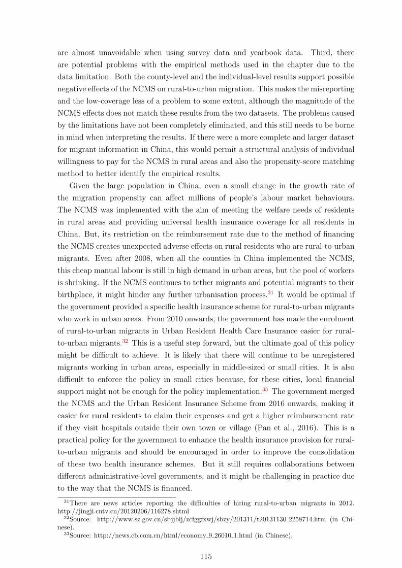
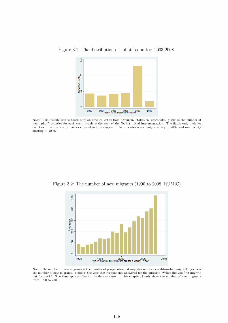
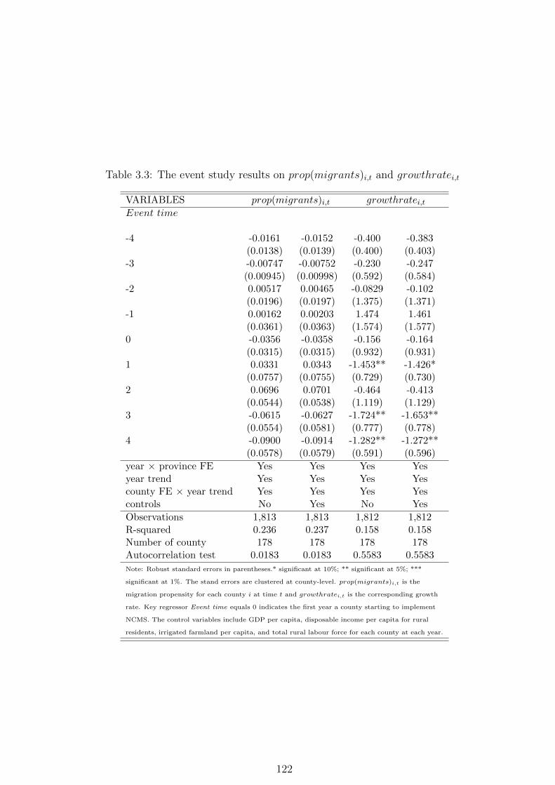
cial yearbooks in China, the results of the event-study approach show that the NCMS

does not reduce the percentage of rural residents who are rural-to-urban migrants and

working outside their home counties at the county level but does have negative effects

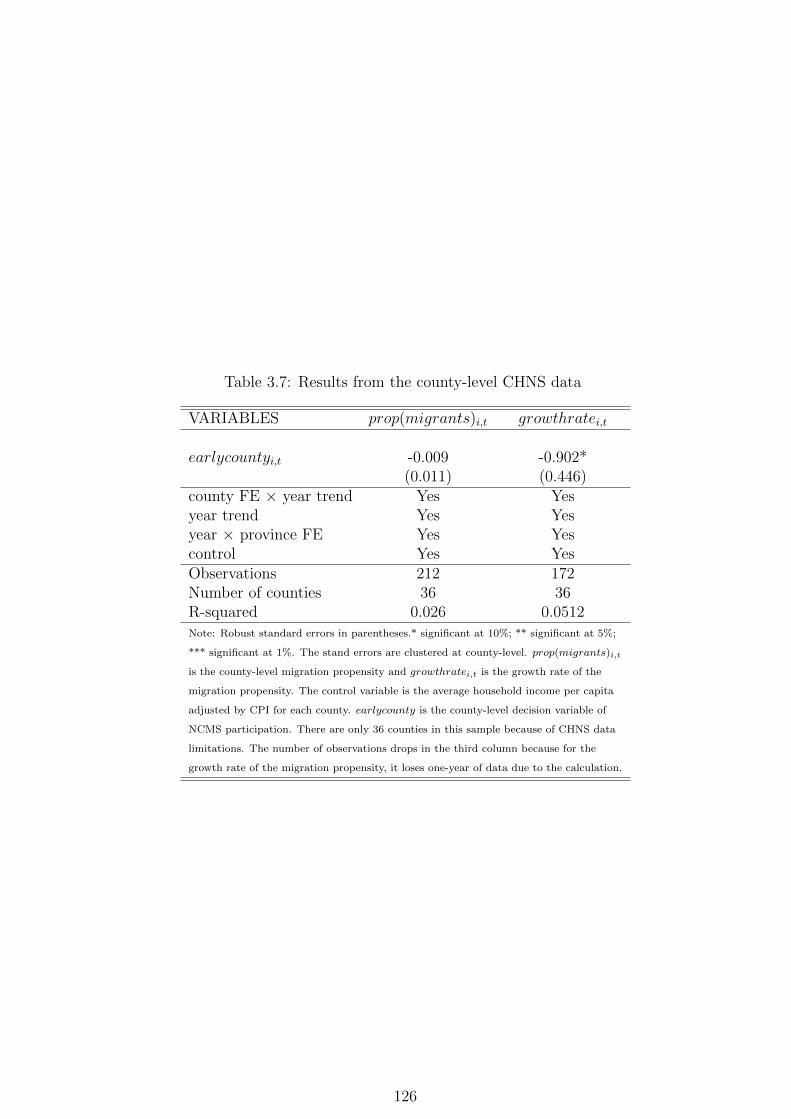
on its growth rate. Using the China Health and Nutrition Survey (CHNS), my instru-

mental variable results find that being enrolled in the NCMS decreases the probability

of being a migrant at the individual level. The IV is a time-variant dummy indicating

the counties that has relative early NCMS implementations. I also used the CHNS to

construct a county-level dataset and replicate the county-level results. Together, the

results suggest that the NCMS gradually locks the rural labour force into rural areas

and further hinders geographical job mobility in China.

iv

Contents

1 The Role of Social Norms in Old-age Support: Evidence from China 1

1.1 Introduction . . . . . . . . . . . . . . . . . . . . . . . . . . . . . . . . . 2

1.2 Background . . . . . . . . . . . . . . . . . . . . . . . . . . . . . . . . . 6

1.2.1 Old-age support in China . . . . . . . . . . . . . . . . . . . . . 6

1.2.2 Indirect reciprocity . . . . . . . . . . . . . . . . . . . . . . . . . 7

1.3 Data and empirical results . . . . . . . . . . . . . . . . . . . . . . . . . 9

1.3.1 Data . . . . . . . . . . . . . . . . . . . . . . . . . . . . . . . . . 9

1.3.2 Main regression . . . . . . . . . . . . . . . . . . . . . . . . . . . 11

1.3.3 Identification strategy . . . . . . . . . . . . . . . . . . . . . . . 13

1.3.4 Main results . . . . . . . . . . . . . . . . . . . . . . . . . . . . . 18

1.3.5 Subsample analysis and heterogeneity check . . . . . . . . . . . 21

1.4 Robustness check . . . . . . . . . . . . . . . . . . . . . . . . . . . . . . 30

1.4.1 Mechanism check . . . . . . . . . . . . . . . . . . . . . . . . . . 30

1.4.2 Panel results: Event study . . . . . . . . . . . . . . . . . . . . . 34

1.5 Welfare analysis . . . . . . . . . . . . . . . . . . . . . . . . . . . . . . . 36

1.5.1 “Missing women”and the old-age support . . . . . . . . . . . . . 36

1.6 Conclusions . . . . . . . . . . . . . . . . . . . . . . . . . . . . . . . . . 37

1.7 Figures and Tables . . . . . . . . . . . . . . . . . . . . . . . . . . . . . 39

2 The Role of Social Norms in Old-age Support: a Theoretical Ap-

proach 61

2.1 Introduction . . . . . . . . . . . . . . . . . . . . . . . . . . . . . . . . . 62

2.2 Literature review . . . . . . . . . . . . . . . . . . . . . . . . . . . . . . 63

2.3 Baseline model . . . . . . . . . . . . . . . . . . . . . . . . . . . . . . . 65

2.3.1 The demonstration effect from different-gender parents . . . . . 70

2.4 Collective household model: the intra-household bargaining . . . . . . . 74

2.4.1 Relaxed intra-household resource allocation condition . . . . . . 78

2.5 Combined model . . . . . . . . . . . . . . . . . . . . . . . . . . . . . . 83

2.6 Conclusions . . . . . . . . . . . . . . . . . . . . . . . . . . . . . . . . . 88

2.7 Figures . . . . . . . . . . . . . . . . . . . . . . . . . . . . . . . . . . . . 89

v

3 Locked out? China’s New Cooperative Medical Scheme and Rural

Labour Migration 90

3.1 Introduction . . . . . . . . . . . . . . . . . . . . . . . . . . . . . . . . . 91

3.2 Background . . . . . . . . . . . . . . . . . . . . . . . . . . . . . . . . . 93

3.2.1 New Cooperative Medical Scheme and other health insurance

schemes . . . . . . . . . . . . . . . . . . . . . . . . . . . . . . . 93

3.2.2 Rural migrants and the hukou system . . . . . . . . . . . . . . 96

3.3 Evidence from the county-level data . . . . . . . . . . . . . . . . . . . . 98

3.3.1 County-level dataset and main variables . . . . . . . . . . . . . 99

3.3.2 Empirical methods and results . . . . . . . . . . . . . . . . . . . 100

3.4 Evidence from the China Health and Nutrition Survey . . . . . . . . . 107

3.4.1 Individual level evidence . . . . . . . . . . . . . . . . . . . . . . 108

3.4.2 County-level evidence . . . . . . . . . . . . . . . . . . . . . . . . 112

3.5 Conclusions . . . . . . . . . . . . . . . . . . . . . . . . . . . . . . . . . 114

3.6 Figures and Tables . . . . . . . . . . . . . . . . . . . . . . . . . . . . . 117

A Appendix of “The Role of Social Norms in Old-age Support: Evidence

from China” 127

A.1 Gender differences of P in old-age support . . . . . . . . . . . . . . . . 127

A.2 Different representations of outcome variables . . . . . . . . . . . . . . 128

A.3 Additional Notes . . . . . . . . . . . . . . . . . . . . . . . . . . . . . . 128

A.4 Figures and Tables . . . . . . . . . . . . . . . . . . . . . . . . . . . . . 129

B Appendix of “The Role of Social Norms in Old-age Support: a The-

oretical Approach” 152

B.1 The baseline model with saving . . . . . . . . . . . . . . . . . . . . . . 152

C Appendix of “Locked out? China’s New Cooperative Medical Scheme

and Rural Labour Migration” 156

C.1 NCMS coverage and the compensating differential model . . . . . . . . 156

C.2 Data imputation . . . . . . . . . . . . . . . . . . . . . . . . . . . . . . 158

C.3 Placebo test . . . . . . . . . . . . . . . . . . . . . . . . . . . . . . . . . 159

C.4 Robustness Checks . . . . . . . . . . . . . . . . . . . . . . . . . . . . . 159

C.4.1 Different lengths of leads and lags . . . . . . . . . . . . . . . . . 159

C.4.2 Comparison between the early-treated group and the late-treated

groups . . . . . . . . . . . . . . . . . . . . . . . . . . . . . . . . 160

C.4.3 Possible determiners of the NCMS implementation date . . . . . 160

C.5 Figures and Tables . . . . . . . . . . . . . . . . . . . . . . . . . . . . . 161

vi

List of Figures

1.1 Public service announcement posters in China . . . . . . . . . . . . . . 40

1.2 Actual gender ratios for the newborns in China: the yearly trend . . . . 41

1.3 Estimated gender ratios for the newborns in China: the yearly trend . . 42

1.4 Actual gender ratios for the newborns in China: by birth order . . . . . 43

1.5 Impact of the gender of the first child on the probability of providing

any old-age support . . . . . . . . . . . . . . . . . . . . . . . . . . . . . 43

2.1 Simple graphical illustration of the basic model . . . . . . . . . . . . . 89

3.1 The distribution of “pilot”counties: 2003-2008 . . . . . . . . . . . . . . 118

3.2 The number of new migrants (1990 to 2008, RUMiC) . . . . . . . . . . 118

3.3 The yearly effects of FirstNCMS on prop(migrants)i,t and growthratei,t

. . . . . . . . . . . . . . . . . . . . . . . . . . . . . . . . . . . . . . . . 119

3.4 Overview of the average migration propensity and its growth rate . . . 120

A.1 Distribution of CHARLS sample counties and districts . . . . . . . . . 130

A.2 Trend assumption for the instrumental variable (DDIV) . . . . . . . . . 137

C.1 NCMS coverage from 2003 to 2008 . . . . . . . . . . . . . . . . . . . . 161

C.2 Coefficients plot for the effects of FirstNCMS on prop(migrants)i,t

and growthratei,t: Five leads and lags . . . . . . . . . . . . . . . . . . 162

C.3 Coefficients plot for the effects of FirstNCMS on growthratei,t: Seven

leads and lags . . . . . . . . . . . . . . . . . . . . . . . . . . . . . . . . 163

C.4 Map of survey regions in the CHARLS . . . . . . . . . . . . . . . . . . 164

vii

List of Tables

1.1 Primary source of support of China’s elderly, 2005 and 2010 . . . . . . 44

1.2 Summary statistics: Key variables . . . . . . . . . . . . . . . . . . . . . 45

1.3 The demonstration effect on the provision of old-age support: OLS . . 46

1.4 The demonstration effect on the provision of old-age support: IV . . . . 47

1.5 Visibility of the provision of financial old-age support . . . . . . . . . . 48

1.6 The demonstration effect on cohabitation . . . . . . . . . . . . . . . . . 49

1.7 Subsample analysis: Income-level . . . . . . . . . . . . . . . . . . . . . 50

1.8 Subsample analysis:: Single-K family . . . . . . . . . . . . . . . . . . . 51

1.9 Subsample analysis: Urban-rural differences . . . . . . . . . . . . . . . . . 52

1.10 Subsample analysis: P with or without brothers (CHARLS) . . . . . . . . . 53

1.11 Heterogeneity Check: Parents’ pension coverage . . . . . . . . . . . . . 54

1.12 Heterogeneity Check: Income of generation O . . . . . . . . . . . . . . 55

1.13 Effects of education and time investment on the provision of old-age

support . . . . . . . . . . . . . . . . . . . . . . . . . . . . . . . . . . . 56

1.14 The demonstration effect on upward and downward transfer . . . . . . 57

1.15 The demonstration effect by generation O . . . . . . . . . . . . . . . . 58

1.16 Impact of the gender of the first child on the probability of providing

any old-age support . . . . . . . . . . . . . . . . . . . . . . . . . . . . . 59

1.17 The “missing girls”and the needs of future old-age support . . . . . . . 60

3.1 Different health insurance schemes and their coverage in China . . . . 121

3.2 The average effects of NCMS on prop(migrants)i,t and growthratei,t . 121

3.3 The event study results on prop(migrants)i,t and growthratei,t . . . . 122

3.4 The effect of the NCMS enrolment on one’s decision to be a migrant . 123

3.5 The first stage for the early county NCMS implementation IV . . . . . 124

3.6 Attrition bias check and attrition-bias-free CHNS data . . . . . . . . . 125

3.7 Results from the county-level CHNS data . . . . . . . . . . . . . . . . 126

A.1 Summary statistics for CHARLS: Females and males subsamples . . . . 131

A.2 Summary statistics for CHFS: Females and males subsamples . . . . . 132

A.3 The gender of the adult child on the provision of old-age support . . . 132

A.4 The demonstration effect on the provision of old-age support: different

cluster levels . . . . . . . . . . . . . . . . . . . . . . . . . . . . . . . . . 133

viii

A.5 First stage for two constructed instrumental variables . . . . . . . . . 134

A.6 The demonstration effect on the provision of old-age support: Dummy

gender ratio . . . . . . . . . . . . . . . . . . . . . . . . . . . . . . . . . 135

A.7 Different representations of the probability and the amount of transfers 136

A.8 Son preference in China . . . . . . . . . . . . . . . . . . . . . . . . . . 137

A.9 The demonstration effect: no cohabitation sample only . . . . . . . . . 138

A.10 Heterogeneity Check: Household income level . . . . . . . . . . . . . . 139

A.11 Heterogeneity Check: Single child family . . . . . . . . . . . . . . . . . 140

A.12 Heterogeneity Check: Urban-rural differences . . . . . . . . . . . . . . 141

A.13 Subsample analysis: Urban-singleton households . . . . . . . . . . . . . 142

A.14 Heterogeneity Check: Family compositions of P . . . . . . . . . . . . . 143

A.15 Heterogeneity Check: Living in a community with minority ethnic groups144

A.16 Heterogeneity Check: Ethnic groups . . . . . . . . . . . . . . . . . . . 145

A.17 The demonstration effect: migrants only . . . . . . . . . . . . . . . . . 146

A.18 The demonstration effect: migrants living with/out K and O . . . . . 147

A.19 The demonstration effect and the education investment in generation K 148

A.20 The demonstration effect without controlling for the transfers from gen-

eration O . . . . . . . . . . . . . . . . . . . . . . . . . . . . . . . . . . 149

A.21 The direct downward transfer from generation O . . . . . . . . . . . . 150

A.22 Subsample check: High and low gender-ratio provinces (after 2003 sam-

ples only) . . . . . . . . . . . . . . . . . . . . . . . . . . . . . . . . . . 151

C.1 The event study results with different s.e. clusters . . . . . . . . . . . 165

C.2 The placebo tests for the effects of the NCMS . . . . . . . . . . . . . . 166

C.3 The effects of FirstNCMS on prop(migrants)i,t and growthratei,t:

with different lengths of leads and lags . . . . . . . . . . . . . . . . . . 167

C.4 The effects of FirstNCMS on prop(migrants)i,t and growthratei,t:

Seven leads and lags . . . . . . . . . . . . . . . . . . . . . . . . . . . . 168

C.5 The effects of FirstNCMS on prop(migrants)i,t and growthratei,t:

Four leads only and four lags only . . . . . . . . . . . . . . . . . . . . . 169

C.6 The effects of the NCMS on the early-treated and late-treated group . 170

C.7 The correlations between NCMS implementation and possible determiners171

C.8 Number of counties implimented the NCMS in the CHNS dataset over-

time . . . . . . . . . . . . . . . . . . . . . . . . . . . . . . . . . . . . . 171

ix

Chapter 1

The Role of Social Norms in

Old-age Support: Evidence from

China

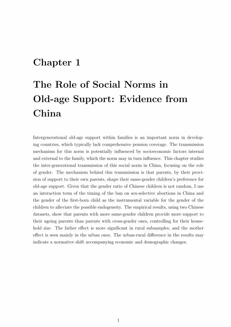
Intergenerational old-age support within families is an important norm in develop-

ing countries, which typically lack comprehensive pension coverage. The transmission

mechanism for this norm is potentially influenced by socioeconomic factors internal

and external to the family, which the norm may in turn influence. This chapter studies

the inter-generational transmission of this social norm in China, focusing on the role

of gender. The mechanism behind this transmission is that parents, by their provi-

sion of support to their own parents, shape their same-gender children’s preference for

old-age support. Given that the gender ratio of Chinese children is not random, I use

an interaction term of the timing of the ban on sex-selective abortions in China and

the gender of the first-born child as the instrumental variable for the gender of the

children to alleviate the possible endogeneity. The empirical results, using two Chinese

datasets, show that parents with more same-gender children provide more support to

their ageing parents than parents with cross-gender ones, controlling for their house-

hold size. The father effect is more significant in rural subsamples, and the mother

effect is seen mainly in the urban ones. The urban-rural difference in the results may

indicate a normative shift accompanying economic and demographic changes.

1

1.1 Introduction

Family support provided by adult children acts as a major income source for ageing

parents in developing countries. This social norm of providing support to the elderly

is traditional and common, especially in China.1 Usually, the norm is gender-specific:

sons provide more support than daughters (Lee et al., 1993). It helps to offset possible

risks and expected income drops for the elderly in countries with underdeveloped public

pension systems and incomplete financial markets. As a large developing country

with an estimated share of the elderly population due to reach 25% in 2030, China is

feeling the weight on its public finances of sustaining, improving, and complementing its

current pension schemes.2 Family old-age support has served as the complement for the

incomplete public pension system in sustaining the welfare of the elderly in China. A

major topic of debate here, with possibly unsustainable pay-as-you-go pension schemes

in the future, has been how the norm of providing old-age support can be transmitted to

future generations. Given the decline in population growth and the potential problem

of ageing in other developing countries, a study of the transmission of social norms

of support for the elderly in China may help many developing countries understand

better how to encourage such support in the future.

This chapter studies the inter-generational transmission of the social norm of old-

age support provision in China, focusing on the same-gender channel. Parents convey

the social norm of old-age support provision to their same-gender children, in the way

that they provide support to their own parents. The hypothesised mechanism behind

this norm transmission is the same-gender “demonstration effect”. It is based on the

demonstration effect established by Cox and Stark (1996). The demonstration effect

means that parents treat their parents well if they have “their own children to whom to

demonstrate the appropriate behaviour” (Cox and Stark, 2005). This inter-generational

demonstration meets the anthropologists’ description of an upward and positive indi-

rect reciprocity (Arrondel and Massaon, 2006). Anthropologists believe the indirect

reciprocity is an important channel of cultural norm transmission (Mauss, 1950, 1968).

I improve Cox and Stark’s demonstration effect by adding the same-gender transmis-

sion channel for two reasons. First, there is good evidence in sociology and psychology

that children are largely influenced by their same-sex parent in their learning of gender

norms in society (Lytton and Romney, 1991; Bussey and Bandura, 1999; McHale et al.,

1999). Economists have recently found empirical evidence for same-gender intergener-

1In the Chinese Household Finance Survey, 74% of the respondents believed that their childrenshould be fully or at least partly responsible for their care in old age.

2United Nations (2015) estimated that, in 2030, the share of the population in China aged60 and older will be 25%. The current share of the population aged 60 and older in the U.K.is 23.9% and in China is 16.2% (United Nations, 2017). The total number of people aged 60or above is 222 million, which is around 4 times the current population of the United Kingdom.WSJ coverage: https://blogs.wsj.com/chinarealtime/2015/03/10/china-sets-timeline-for-first-change-to-retirement-agesince-1950s/. In 2017 China raised the retirement age, set in the 1950s, to alleviatepressures on its public finances.

2

ational transmissions in individual preferences and social norms (Alesina et al., 2013;

Kleven et al., 2018). The second reason is that the gender difference is prominent in

the norm of old-age support provision in China and other developing cultures (Gupta

et al., 2003). Traditionally, sons are responsible for supporting their elderly parents in

China (Lee et al., 1993; Chan et al., 2002).

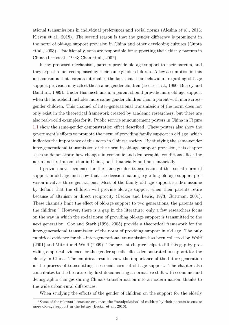
In my proposed mechanism, parents provide old-age support to their parents, and

they expect to be recompensed by their same-gender children. A key assumption in this

mechanism is that parents internalise the fact that their behaviours regarding old-age

support provision may affect their same-gender children (Eccles et al., 1990; Bussey and

Bandura, 1999). Under this mechanism, a parent should provide more old-age support

when the household includes more same-gender children than a parent with more cross-

gender children. This channel of inter-generational transmission of the norm does not

only exist in the theoretical framework created by academic researchers, but there are

also real-world examples for it. Public service announcement posters in China in Figure

1.1 show the same-gender demonstration effect described. These posters also show the

government’s efforts to promote the norm of providing family support in old age, which

indicates the importance of this norm in Chinese society. By studying the same-gender

inter-generational transmission of the norm in old-age support provision, this chapter

seeks to demonstrate how changes in economic and demographic conditions affect the

norm and its transmission in China, both financially and non-financially.

I provide novel evidence for the same-gender transmission of this social norm of

support in old age and show that the decision-making regarding old-age support pro-

vision involves three generations. Most of the family old-age support studies assume

by default that the children will provide old-age support when their parents retire

because of altruism or direct reciprocity (Becker and Lewis, 1973; Guttman, 2001).

These channels limit the effect of old-age support to two generations, the parents and

the children.3 However, there is a gap in the literature: only a few researchers focus

on the way in which the social norm of providing old-age support is transmitted to the

next generation. Cox and Stark (1996, 2005) provide a theoretical framework for the

inter-generational transmission of the norm of providing support in old age. The only

empirical evidence for this inter-generational transmission has been collected by Wolff

(2001) and Mitrut and Wolff (2009). The present chapter helps to fill this gap by pro-

viding empirical evidence for the gender-specific effect demonstrated in support for the

elderly in China. The empirical results show the importance of the future generation

in the process of transmitting the social norm of old-age support. The chapter also

contributes to the literature by first documenting a normative shift with economic and

demographic changes during China’s transformation into a modern nation, thanks to

the wide urban-rural differences.

When studying the effects of the gender of children on the support for the elderly

3Some of the relevant literature evaluates the “manipulation” of children by their parents to ensuremore old-age support in the future (Becker et al., 2016).

3

provided by their parents in China, an empirical difficulty is that the gender of the

children is endogenous. The increasing gender ratio of newborns in China corresponds

to the imbalance in the gender ratio of the children in the datasets. The gender ratio of

new-borns has been increasing since 1990 (China Population and Employment Statis-

tics Yearbooks, Figure 2). For this, sex-selective abortion is one of the main reasons

(Chen et al., 2014). The non-random gender ratio of the children could positively or

negatively affect the support for the elderly provided by parents.4 To address this

problem, I utilise two facts: the gender of the first child in households and the timing

of a policy ban on sex-selective abortions.

I use the interaction term of the gender of the first child in a household and whether

or not a household is affected by the policy ban as the instrumental variable (IV) for

the gender ratio of the children. This IV exploits two facts. First, the gender of

the first child is closer to the natural rate than the gender ratio for all new-borns in

China (Ebenstein, 2010; Wei and Zhang, 2011). Scholars usually regard the gender

of the first child as random (Jayachandran and Pande, 2017; Heath and Tan, 2018).

However, given the highly skewed gender ratio of newborns in China, it is difficult

to concede that the gender of first-born children is fully exogenous. Second, a policy

was introduced to reduce the gender ratio to its natural level, so the gender of first-

born children who were born in or after the year of the policy ban is approximately

close to the natural rate. The policy banned the use of ultrasound for prenatal sex

determination and imposed fines on those who conduct sex-selective abortions. It was

initiated by the National Family Planning Commission (NFPC) in 2003 affecting all

households that have at least one child born in or after 2003.

The timing of the policy change is plausibly exogenous at household-level.5 I find

that the policy, as intended, negatively affects the household-level gender ratio of chil-

dren. The compliers are those who have not conducted sex-selective abortions since

the policy ban. Usually, they prefer sons to daughters. There are two different types of

complier: affected and unaffected. The affected compliers are those who have children

of the opposite sex to their wishes. They capture the time variation of the policy. For

example, after 2003, the affected compliers who would have been willing, had no ban

existed, to conduct sex-selective abortions, have daughters, and this decreases the gen-

der ratio of their children. Unaffected compliers who have sons after 2003 by natural

chance provide no variation. The gender ratio of the children of people who would not

conduct a sex-selective abortion in any circumstances cannot be affected by this policy,

and the gender ratio in their households should be close to the natural rate. The IV

thus captures the differences for the affected compliers before and after the policy ban.

The main empirical findings indicate that parents increase probabilities of providing

financial and non-financial support in old age with more same-gender children, con-

4This will be further elaborated in the empirical results section.5The law-making processes of most Chinese policies are quite exogenous, as far as members of the

public are concerned (Hu, 1998; Shen, 2008).

4

trolling for the household size. I only compare the difference within parents’ gender

for the old-age support provided by them. In the datasets, the father and the mother

both show gender-specific demonstration behaviours. The results from the robustness

check and the heterogeneity analysis are mostly consistent with the expected results

under the demonstration effect channel. The ‘father’ demonstration effect is generally

more significant in low-income and rural subsamples, and also in households with more

than one child. The ‘mother’ effect is most significant for the outcome variables in low-

income and urban subsamples. The empirical evidence implies that support for the

elderly is closely linked to the composition of the gender of parents and their children,

which suits the assumption that the norm of providing support for the elderly is likely

to be transmitted to offspring of the same gender.

However, the two datasets exhibit different gender-dominated demonstration be-

haviours. The CHARLS (the China Health and Retirement Longitudinal Study) mainly

presents the father demonstration effect. The mother effect has a more substantial role

in the urban subsample and also in the whole sample of the CHFS (the China House-

hold Finance Survey). One explanation for this difference is because the CHARLS

contains more rural samples than the CHFS. It is consistent with results from the

urban-rural heterogeneity analysis and subsample check. The discrepancy between the

urban and rural subsample results has implications for the norm-shift of providing sup-

port for the elderly together with the development of China. Urban areas in China are

more developed than rural areas: they have higher pension/insurance coverage, better

public infrastructure, and, in particular, fewer gender inequalities and higher female

bargaining powers (Fong, 2002; Lee, 2012). The results may suggest that higher female

household bargaining power may lead to more significant mother demonstration effects.

The mechanism checks also show that the existence of other possible mechanisms, such

as altruism and direct reciprocity, is not likely to affect the demonstration effect mech-

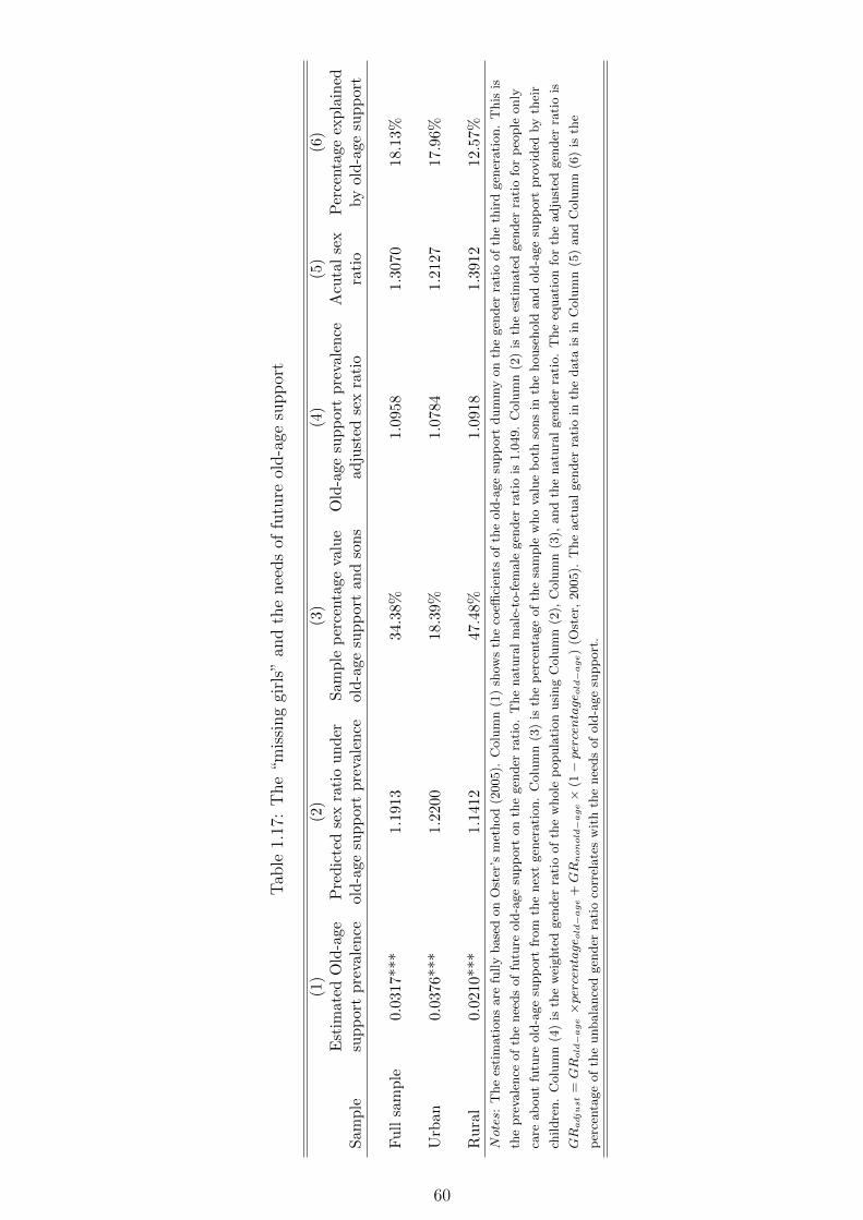
anism in the results. I also calculate the correlation between the “missing girls” and

the demand for support for the elderly in a patrilineal society, using a method from

Oster’s 2005 paper. Using this method, I calculate the adjusted sex-ratio based only

on the correlation between the unbalanced gender ratio and the demand for support

for the elderly from sons. The demand for old-age support accounts for 12-18% of the

unbalanced gender ratio in the data.

The chapter proceeds as follows. More background information on support for the

elderly from children in China is in Section 1.2. Section 1.3 provides the theoretical

background for the same-gender social norm transmission and the model. This is

followed by Section 1.3, which provides the identification strategy and the empirical

findings. Section 1.4 also provides the robustness check for the key empirical findings.

Section 1.6 offers some concluding thoughts.

5

1.2 Background

1.2.1 Old-age support in China

The provision of financial and non-financial support to ageing parents is a pro-social

norm in China and other countries that are influenced by Confucianism. This family

support for the elderly has been acting as an alternative way of sustaining the welfare

of elderly to the incomplete public pension system. Table 1.1 shows that in 2005

less than 50% of the urban elderly viewed public pensions as their major source of

income. In rural areas, the percentage was only around 5%. More than 50% of the

rural elderly and around 40% of their urban counterparts believed their major source

of income to be family support. Even with the development of the public pension in

both urban and rural areas in China, the percentage of rural elderly choosing pensions

as their main income source in 2010 was unchanged, although the percentage of those

who chose family support declined to 47%. The pension schemes in urban areas have

been improved since 2005: around 70% of the urban elderly in 2010 relied on a public

pension while only around 20% of them lived mainly on family support. Inferring from

the statistics, the public pension coverage shows a wide urban-rural difference. Rural

areas in China do not seem to have had an effective pension scheme before 2011, so

the elderly there were still depending on the norm of private support for the elderly.

A large proportion of the elderly in China live on support from their family mem-

bers, especially from their adult children. The social norm of providing support for the

elderly is then important to those who try to secure their income after their retirement.

First, they have to know which characteristics affect the amount of support that they

can depend on in old age. The number and the gender of the adult children are two

major aspects studied in the relevant literature on China. In the standard old-age

support literature, such as Becker and Lewis (1973), people believe that more children

in a household will lead to more support for the elderly in the future. Cai et al. (2006)

and Oliveira (2016) both verify this common belief among Chinese people. As regards

the gender of the children, traditionally, males are responsible for providing support to

their parents in their old age. Hence the early literature assumed that males provide

more than females due to cultural and labour market restrictions (Lee et al., 1993;

Chan et al., 2002). The value of male offspring in providing support for the elderly is

one of the reasons behind the persistent preference for sons in China and other devel-

oping countries (Gupta et al., 2003). It was common in China for households to have

at least one son, right up to the implementation of the “One-Child” Policy (OCP)

(Milwertz, 1997; Ebenstein and Leung, 2010). However, in the recent literature, Xie

and Zhu (2009) find that females were providing more support to elderly parents in

urban areas, and Oliveira (2016) finds no gender differences in the provision of support

in old age. But given the rising gender ratio for newborns in China, especially in rural

areas, it is reasonable to assume that this gender difference still exists, though it may

6

vary between rural and urban areas.

Once those who rely on family support for income in old age know the factors af-

fecting their future income, it is highly likely that they will try to manipulate these

characteristics. For most families in China, the number of children is difficult to ma-

nipulate. With the strict implementation and high fines of the OCP, Ebenstein (2010)

has found that the policy reduced fertility. Gender, however, was a characteristic that

was easier for people to manipulate, with the help of advanced technologies. Chen et al.

(2013) have inferred that the increasing gender ratio could be attributed to increased

gender selection before birth, thanks to gender-selection technology. For example, B-

mode ultrasound allowed people to know the sex of a foetus and was in common use

all over the world after 1980 (White, 2001). Qian (2008) has discovered that an in-

creased future income for females also improved the female survival rate. In addition,

Ebenstein and Leung (2010) have studied the effects of having a public pension system

on the sex ratio at birth in China. They find that when a region is covered by a public

pension scheme, its gender ratio is more balanced than it is in regions without such

coverage. From the literature, it seems that in China, gender is a key factor in the

norm of family support in old age. Support for the elderly is also, important enough

to affect fertility decisions, such as the number and gender of people’s future children.

Parents internalise future support that they will receive from their children when they

are old and try to alter the characteristics that might affect their own future support.

1.2.2 Indirect reciprocity

It is important to learn how to best support the elderly, given their situation. First, we

should understand the possible mechanisms for doing so. Altruism and exchange are

the two main motives in the standard theoretical models analysing intergenerational

transfer. Altruism, in the context of, support for the elderly means that people are

generally willing to support their ageing and retired parents. The theoretical framework

for altruistic individuals is developed by Barro (1974) and Becker (1976, 1981). The

exchange mechanism is also referred to as (direct) reciprocity. It describes support for

the elderly as reciprocal payments for the financial and/or non-financial investment

made in the donors’ childhood (Cox, 1987). However, the existing empirical results are

not robust enough to support these two motives in theoretical models (Arrondel and

Masson, 2006). The theory of indirect reciprocity may serve to reconcile the motives

of altruism and exchange. Indirect reciprocity is also the theoretical support for the

inter-generational transmission of the norm of giving support to the elderly.

The concept of indirect reciprocity is usually attributed to Mauss (1950, 1968), a

French anthropologist. He expands the common “gift-return” reciprocity relationship

between two parties, the giver and the beneficiary, to three parties. He states that

indirect reciprocities involving three successive generations will lead to infinite chains

of transfers. He observes that the givers do not get direct payback from the beneficiary

7

but receive it from a third person (Arrondel and Masson, 2001). The channel works for

any type of transfer: upward, downward, positive or negative. Cox and Stark (1996)

provide a model to describe similar behaviours in the provision of support in old age,

which coincides with the upward and positive indirect reciprocity channel. In the

context of support for the elderly, the interaction between three parties is that parents

educate their children by providing support for the elderly to their parents so that the

parents when elderly will receive support from their children. It is usually referred to as

the “demonstration effect”. The model predicts that transfers from individuals to their

parents are positively affected by the presence of their children. Cox and Stark (2005)

test the prediction using U.S. data. Wolff (2001) and Mitrut and Wolff (2009) also

find that the existence of granddaughters increases the visits paid to the grandparents;

Becker et al. (2016) believe that parents can “manipulate” the preferences of children,

an assumption underlying the demonstration effect.

Bau (2019) studies the connection between the cultural norm and support for the

elderly in Ghana and suggests that support for the elderly is a product of cultural

norms. Except for Mitrut and Wolff (2009), the relevant literature considers only the

role of the children in the transmission of the norm of old-age support, without any

consideration of the role of gender. Given the gender difference regarding support for

the elderly and preference in China for sons, the demonstration effect may also be linked

with the gender of the third generation. Godelier (1982) describes indirect reciprocity

as gender-specific when it functions as a channel for the transmission of cultural traits

and norms. If there is a gender-specific social norm, then it is also a channel for passing

on gender norms in society. Mitrut and Wolff (2009) find that parents’ visits to their

own parents are largely affected by the presence of daughters rather than sons in their

households. This empirical finding is consistent with common beliefs about the role of

gender: parents of girls are the more likely ones to pay visits and care for the elderly

(Lee et al., 1993).

If providing support for the elderly links with gender norms, one vital assumption

is that parents should be able to influence their same-gender children more effectively

than cross-gender children. Children would also mimic the behaviour of the same-

gender parent in the future, a phenomenon which is known in psychology and sociol-

ogy as “gender socialisation/specification”. Many sociologists and psychologists believe

that the same-sex parent is the main source for ensuring that children to learn the cor-

responding gender role that fits social expectations and that the children will perform

gender-related behaviours when they become adults (Lytton and Romney, 1991; Bussey

and Bandura, 1999; McHale et al., 1999). In the recent economics literature, several

papers focus on same-gender intergenerational transmission. Jayachandran and her

colleagues show that the effects of the same-sex parent on gender attitudes are greater

than the peer effects (Dhar et al., 2018). Kleven et al. (2018) reveal that in Denmark

preferences over family and career for females are largely influenced by the mother’s

8

preference observed during childhood. Alesina et al. (2013) also find that paternal

ancestors affect the perspectives of males on the gender role and the female labour

market participation.

Parents should also internalise the fact their children’s future behaviours will be

affected by theirs. This internalisation means that parents will begin to influence

their offspring in order to form their children’s preferences. Becker (1996), Bisin and

Verdier (2000), Guttman (2001), Bronnenberg et al., (2012), and Becker et al. (2016)

study whether parents show certain behaviours to or spend more resources on their

children in order to formalise their children’s preferences. After listing the relevant

evidence supporting the demonstration effect and same-gender intergenerational norm

transmission, it is reasonable to assume that the demonstration effect works in a more

gender-specific way when there is a wide gender difference in the planned support for

the elderly. People will demonstrate the norm of support in old age to their same-

gender offspring by providing support for the elderly to their own parents. Figure 1.1

provides examples in China for the same-gender demonstration effect.

1.3 Data and empirical results

1.3.1 Data

Two datasets are used to assess the gender effects of children on the norm transmission

of old-age support, more specifically, how the gender of children affects the support

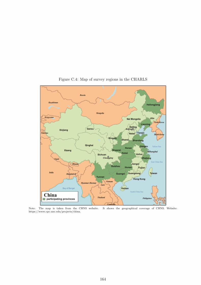
for the elderly provided by their parents. The first dataset is the China Health and

Retirement Longitudinal Study (the CHARLS). The CHARLS is a longitudinal survey

of 28 out of the 34 provinces of the country for three waves in the years 2011, 2013 and

2015 up to the present day.6 It collects a representative sample of residents aged 45 or

above. The main wave used in this chapter is the 2011 wave. The data set contains

information on each respondent’s family, work, retirement, wealth, health and income.

The main demographic group in the survey is people aged 45 or above. In the 2011

sample, this covered about 17,708 individuals in 10,257 households from 28 provinces.

The sample was randomly selected from four samplings at different levels: county-level,

neighbourhood-level, household-level and respondent-level.7

The CHARLS provides detailed information on inter-generational and inter-household

transfers. One advantage of this dataset is that it clearly distinguishes between the

transfers from each child of the respondents. The survey also identifies different types

of support, whether regular or non-regular. The regular support acts as income re-

ceived from the children of the respondents at fixed times. Regular support is similar

to the support for the elderly as defined: a certain amount of income paid repetitively

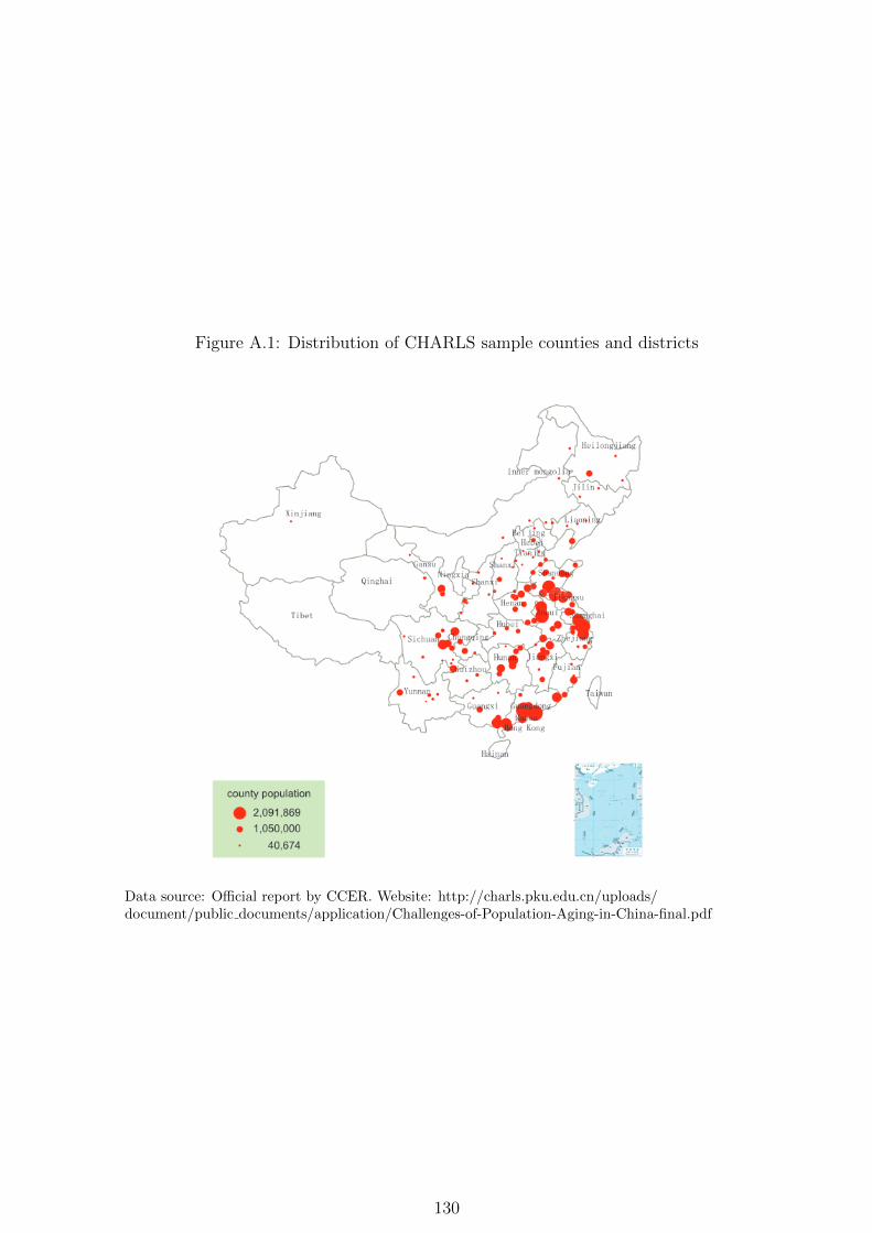
6The detailed distribution in provinces and counties is presented in Figure A.1.7The detailed sampling method at each level can be accessed at:

http://charls.pku.edu.cn/en/page/about-sample-2011.

9

to the elderly at a fixed time. Non-regular support is the support provided at different

times of the year and is not necessarily repetitive, whereas the regular one is.8 Given

the high average age of the respondents, the sample size for the available observations

in terms of the transfer provided by the respondents to their parents is small. But

many of the respondents have children of working age, so most of them receive support

from their children. I regard the support for the respondents provided by their children

as the support from parents to their elderly parents discussed in the previous section.

The respondents in the survey are the passive recipients of old-age support. Namely,

they are the elderly the main regressions in the CHARLS. The grandchildren of the

survey’s respondents are the children of the respondents’ children.

To fit the original dataset into my setting, I construct a new sample that cov-

ers the adult children of the survey respondents, namely, the parents.9 In the newly

constructed sample, the sample size decreases to about 14,000 observations. In the

reconstructed 2011 wave, around 65% of people come from rural areas, and more than

75% of them have rural hukou (“household registration”). However, due to the ques-

tionnaire design of the CHARLS, the demographic information on the parents and their

children is not as detailed as the information on their elderly parents in my regression.

The available demographic variables in the 2011 wave about the children are only the

gender and the number of them. In the 2013 and 2015 wave, the only available demo-

graphic variable is the number of the children. This is the reason why I can conduct

only cross-sectional analyses when using the CHARLS.

I used a second dataset to verify the generalisation of the results from the CHARLS

and also to provide supplementary evidence for the demonstration effect. The dataset

is the China Household Finance Survey (the CHFS). The CHFS is a panel dataset

covering 25 provinces in China, by Southwestern University’s Department of Finance

and Economics and Research Institute of Economics and Management. This survey

focuses on household-level financial behaviours. It currently has three waves: for the

years 2011, 2013, and 2015. The survey does not have the same age limitation on the

survey respondents as the CHARLS does; hence, there is no need to reconstruct the

dataset. In the CHARLS, I treated the main respondents of the survey as the parents.

The sample in the 2011 wave includes only 8,438 households, and its questionnaire

includes only the gender of the children who are living together with the respondents.

In the 2013 wave, the number of observations increased significantly: 28,142 households

and 97,916 individuals. Accordingly, I used the 2013 wave in the CHFS for more

observations and more precise information on the gender ratio of the children and

old-age support provided.

I include only the main respondent for each household in my CHFS sample for

regression. The main respondents know the household financial situation best (Li et

8In the CHARLS, non-regular support is defined as “support at Spring Festival or/and Mid-Autumn Festival or/and birthday or/and wedding or/and funerals or/and others”.

9A detailed discussion of the dataset reconstruction is in Appendix A.3.

10

al., 2015). They are responsible for answering the household-level financial questions,

which includes the questions regarding inter-household transfers. If I included only the

main respondents, there would be a selection bias. In this sample, the parents are in

charge of household finances. So, one possible effect would from females who were in

charge of the household finances, who may have a higher power in their household than

is held by females who are not in charge. A possible result of this selection would be

that the females in my CHFS sample transferred more to their parents, which makes my

CHFS results an upper bound of the female demonstration effect. However, regarding

the households’ support for the elderly, the main respondents may know only the exact

amount of their own transfers, and not that of their partner. Their partner may hide

the information from them (Ashraf, 2009). Moreover, only the main respondents have

information about their own parents. The 2013 wave also includes the gender of all the

children of the respondents. One limitation of the CHFS is that the information about

the intergenerational and inter-household transfer collected in the survey is not as

detailed as the information available in the CHARLS. Each dataset has its advantages

and disadvantages. A comprehensive interpretation of the results from both datasets

is necessary.

1.3.2 Main regression

The chapter sets out to examine the gender effects of the children on the support for the

elderly provided by their same-sex parent. The main regression includes the gender of

the parents, the gender ratio of their children in their household, and their interaction

term. The main regression is:

yi = α + βsex ratioKi + γmalePi + δ(malePi × sex ratioKi) + X′iθθθ + φc + εi. (1.1)

In the equations, i stands for a parent i. yi represents the outcome variables testing

various aspects of old-age support. The error term is εi is clustered at the prefecture

city-level for the CHARLS and the province-level for the CHFS.10 The different cluster-

levels for the CHARLS and the CHFS is because the CHFS does not provide any

information on prefecture cities. φc is the province fixed effects. For the main regressors,

I use the three-generation setting: P is the parents, K represents the children of P ,

and O is the parents of P . malePi is the gender of a parent i in the P generation.

It equals 1 if the parent is male and 0 otherwise. The regressor sex ratioKi is the

actual male-to-female gender ratio of the children in parent i’s household. The gender

ratio of K equals the number of sons for a parent i divided by the total number of

K in the household if i has more than one child. For i with one child, if the only

10The results are similar when the error terms clustered at the individual-level and also the province-level. The choice of the cluster level is discussed in the following section discussing the instrumentalvariable.

11

child is a boy, then sex ratioKi = 1. If the only child is a girl, then sex ratioKi = 0.

sex ratioKi×malePi is the interaction term, and Xi is the set of demographic variables

for P and O to be controlled for in the regression.11 I run separated regressions for

the CHARLS and the CHFS, since the difference between the two datasets is quite

large. Using this regression equation, I manage to calculate the within-parent gender

differences in terms of providing support for the elderly caused by the gender ratio of

their children, while controlling for the P ’s own gender and household-size.

There are three consistent main outcome variables in both two data sets. They are

the dummy indicating whether P provide any financial transfer to O (any-transfer),

the amount of any transfer provided (amount), and the number of days spent on P ’s

visits paid to O per year (visit days). The transfers provided to P ’s parents are the

pecuniary old-age support provided. For the amount of the transfer, I unify it to the

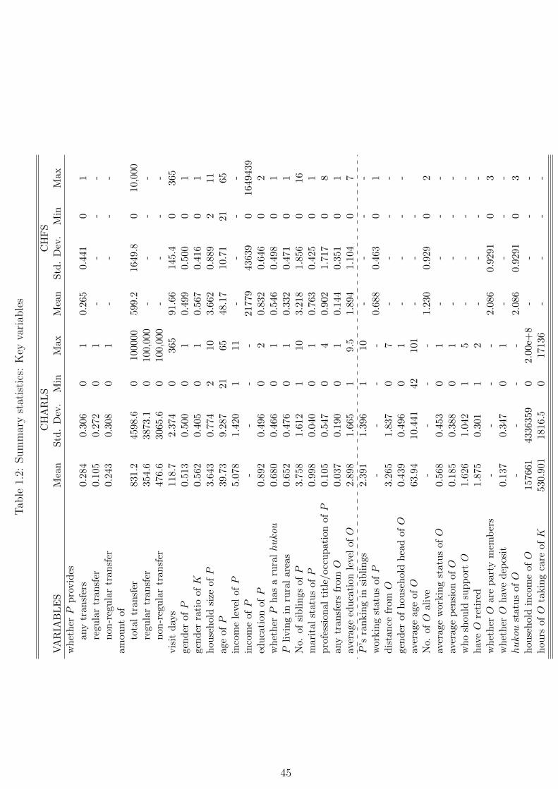
annual amount and the amounts are capped.12 The summary statistics for the outcome

variables, key regressors, and control variables in different datasets are shown in Table

1.2.13 In the CHARLS questionnaire, transfers are classified into two different types:

regular transfer and non-regular transfer. The regular transfer is the fixed-amount

transfer that parents make to their elderly parents at fixed times. The non-regular

transfer represents transfers provided by the parents at non-regular but important

social events or circumstances. These two types of transfers are not used in the main

analysis, but in the check parts only. The amount of any transfer provided in the

CHARLS is the sum of the regular and the non-regular transfer.

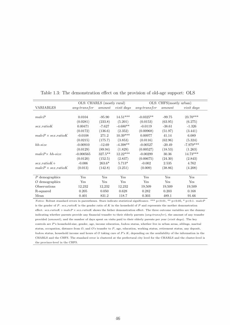
The OLS results from Equation (1.1) for the CHARLS and the CHFS are shown in

Table 1.3. Before analysing the gender effects of children, I first want to verify whether

there are gender differences in the provision of support for the elderly by the parents

in the CHARLS and the CHFS. In the recent literature, it seems that males no longer

provide more old-age support than females (Xie and Zhu, 2009; Oliveira, 2016).14 I

want to use the simple OLS regressions with maleP as the only key regressor to check

whether the male P provide more in the datasets used. The corresponding results in

Table A.3 might imply that there are certain gender differences of P in old-age support.

The coefficients of maleP are similar to the corresponding coefficients in Table 1.3. The

detailed discussion about the gender differences of P in old-age support is in Appendix

Section A.1.

For the main results in Table 1.3, they suggest that most of the effects of the

gender of K on old-age support are insignificant. From now on, I refer to females in

11The controls are different in the CHARLS and the CHFS. I try to make the controls consistentbetween the two datasets. The control variables for O are more in the CHARLS than in the CHFS,but information on P and K is more precise in the CHFS.

12The amount of transfers are capped at 100,000 per year in the CHARLS and 10,000 in the CHFS.13The full summary statistics for all the controls and the summary statistics by gender of the adult

children are in the Appendix, Tables A.1 and A.2.14Oliveira (2016) shows that there is no gender difference in the support for the elderly provided

by parents. Xie and Zhu (2009) show that females in urban areas provide more to their parents thanmales do.

12

the P generation as mothers, and their male counterparts as fathers. I only focus on

the gender effects of K within a certain gender of P . In Equation 1.1, −β indicates,

for mothers, the change of old-age support provision corresponding to decreases in the

gender of K in their households. The decrease in the gender of K means there are more

daughters in one’s household, controlling for the total household size. So I name −β as

the mother demonstration effect. β+δ shows the same change for fathers corresponding

to increases in the gender of K in their households, which is the father demonstration

effect. If the same-gender channel works, the expected coefficients of β should be

negative and significant for the mother demonstration effect. The coefficients of β + δ

should be positive and significant to show the father effect. For outcome variables in

the CHARLS, the coefficients of sex ratioK, which is β, for visit days is negative and

significant. The mother and father demonstration effect on the probability of providing

any transfer are insignificant. The father demonstration effects are significant for visits

paid and the amount of transfer. The coefficients for β and β + δ are all insignificant,

yet the signs mostly fit the prediction of the same-gender effects in the CHFS results.

I also include the coefficients for the P household size in the results in Table 1.3.

A large household size implies more children in one’s household. For a mother, an

increase in household size has possible negative effects on her provision of old-age

support, financially or non-financially. But these effects are only significant for the

visits paid to her parents in both datasets. A father, on the other hand, an increase in

his household size have positive effects on the amount of his support provided and the

visits paid to his parents. These positive effects are significant for the visits paid to his

parents in both datasets and for the amount of old-age support in the CHARLS. The

impacts of household-size on fathers are consistent with the demonstration effect by

Cox and Stark (1996): people provide more old-age support if they have more children

in their households. The household size is another important factor that might affect

the decision of gender selections, which is a problem that I would discuss more in the

subsample check section, so controlling the household size and its interaction term with

maleP might help to alleviate the possible selections.15

1.3.3 Identification strategy

The OLS results in both datasets do not appear to support the proposed demonstration

effect. It may be that the results under the OLS model suffer from biases caused by

various possible endogenous problems. One main endogeneity problem comes from the

gender selection issue affecting the gender ratio of the children, sex ratioK. According

to the China Population and Employment Statistics Yearbooks, the yearly national-

level gender ratio of new-borns has been increasing since the late 1980s.16 The national

15It would be more desirable if I can use calculate a counter-factual household size without itscorrelation with the household gender ratio using Qian’s method in her paper ”Quantity-Quality andthe One-Child Policy: the Only-Child Disadvantage in School Enrolment in Rural China”.

16The yearly national-level gender ratio of new-borns is shown in Figure 1.2.

13

gender in 2011 shows the ratio of boys to girls to be as high as 1.25 to 1, revealing

the gender selection problem as quite severe. Households with son preference would

be likely to conduct selective abortions, and these are usually the households holding

the traditional stereotypes of daughters. Households with modern views on gender

equality are less likely to select their children’s gender. In my sample, the gender ratio

of the parents is almost free from this problem. In the CHARLS the average age of

the parents in the sample is 40 and in the CHFS, it is 48. It is around 0.51 in both

datasets. When they were born, gender selection technology was not yet available in

China (Chen et al., 2013). The endogeneity problem of sex ratioK is a larger one, and

it may affect the OLS outcomes in two opposite ways as illustrated by males with a

preference for sons. First, if a male is eager to have a boy only to secure his own future

support, then gender-selection will lead to an upward bias for the father demonstration

effect. Second, if, alternatively, a father wants to have a boy to enhance the household’s

prosperity, he will invest more family resources in a son’s upbringing. So the father

effect is downwardly biased. The effect of the endogeneity is ambiguous in this setting.

To alleviate the bias, I use the timing of a regulation announced in late 2002 by the

Ministry of Health, State Food and Drug Administration (SFDA) together with the

National Family Planning Commission (NFPC). The regulation bans the use of B-scan

ultrasonography and other technologies for determining foetal sex from January 1st

2003.17 It states that all methods of gender selection should be banned and imposes

fines for different levels of violation of the regulation. Fines are imposed on individuals

who choose the sex of a foetus allowed to survive and on the hospitals that conduct

scans and abortions. The policy was intended to make the gender of the children born

in or after 2003 closer to the natural birth rate relatively random, which is lower than

the gender ratio of the children born before. The policy was designed to reduce the

gender ratio of new-born males to females, so it would be relevant to the average gender

ratio of children in households, which is the variable sex ratioK in the main regression

equation. Figure 1.3 shows the estimated yearly gender ratios of new-borns using the

2011 wave in the CHARLS and the estimated yearly gender ratios of the first-born

children using the 2013 wave in the CHFS. This graph shows that both gender ratios

fall after the year 2003.

I use mainly the timing of the policy change to construct the first part of the

instrumental variable employed in the chapter. The policy covers most of the provinces,

and the provincial congresses passed the policy at much the same time,18 with no great

time difference between them. I assign the value of the policy timing variable to 1 for

P with at least one child born in or after 2003, and 0 otherwise. The increasing gender

ratio of male to female new-borns is a heated social issue that usually attracts public

17Website: http://www.gov.cn/banshi/2005-10/24/content 82759.htm. Last accessed: September2018.

18 The provincial congresses all passed the policy at some time between November 2002 and January2003. The information was collected from the provincial government websites.

14

attention. So public discussion may accompany the agenda-setting process of the policy.

However, Hu (1998) and Shen (2008) declare that detailed information and plans are

rarely revealed to the Chinese public in the policy planning stage. Thus, the timing of

the policy implementation is exogenous to the general public. Regarding this policy,

in particular, most of the news about it on Baidu.com or Google.com appears after

the provincial governments or the central government passed the associated regulation.

Also, the policy ban on gender-selective abortions is designed mainly for adjusting the

high male-to-female gender ratio for the newborns in China.19 The exclusion restriction

of using the policy variation is satisfied policy-wise because the policy design does not

include the concern of the old-age provision. However, people might still violate this

policy ban and pay high fines to conduct gender-selective abortions. This could, in turn,

affect that total expenditure of the households, and affect old-age support provision

due to household budget limitations. To conclude, the exogeneity assumption of the

policy timing is reasonable in my setting.

Although Figure 1.3 shows the gender ratio in the CHARLS and the CHFS de-

creased after 2003, the situation is not quite the same as in Figure 1.2. The national

gender ratio has been stagnating at a high level since 2003, although it has not in-

creased since then. Figure 1.2 implies a slight chance that the policy does not ban

sex-selective abortions outright.20 To address this concern, I combined the dummy

indicating the timing of the policy implementation together with the gender of the

first-born child in the households surveyed. The gender ratio of the oldest child in a

family is relatively balanced in China. The One-Child Policy (OCP) does not strictly

require all households to have only “one child”, especially in rural areas, so the first

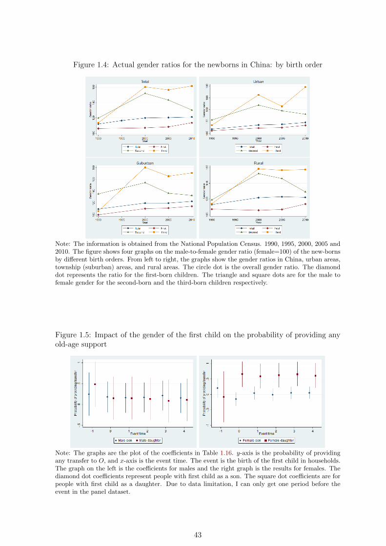
child’s gender is relatively close to the natural ratio of new-borns (Ebenstein, 2010). In

Figure 1.4, the graphs show the ratio of new-born boys who are not the eldest to their

girl counterparts are all larger than the gender ratio among first-born babies. For the

relevance condition for this variable, the gender of the oldest child is usually correlated

with the gender ratio of children in households (Angrist and Evans, 1998; Heath and

Tan, 2018). But the male-to-female ratio for the first-born child is still higher than the

natural rate. Together with the timing of the plausible exogenous policy, my instru-

mental variable can plausibly satisfy the exclusion condition. The IV is an interaction

term of two dummies: one dummy equals 1 for households with at least one child born

in or after 2003 and one dummy equals 1 if the oldest child in a household is a son.

This instrumental variable borrows the concept of the instrumented difference-in-

differences design (DDIV) (Dulfo, 2001; Hudson et al., 2017).21 The key variation

19http://www.gov.cn/banshi/2005-10/24/content 82759.htm20Because the policy did not make the gender ratio of new-borns completely random, I cannot use

the subsample of households with new babies in or after 2003 to test the demonstration effect.21Using of the interaction term of the gender of the first child and whether a household is affected

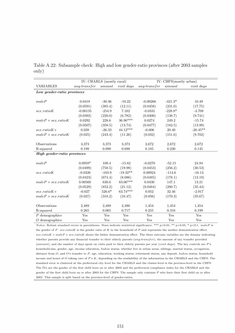
by the policy as IV is necessary. I cannot use only the subsample of households that are affectedby the policy ban when using the gender of the first children as IV. This is because, even with thepolicy ban, the gender ratios in some provinces are still higher than the natural rate. A more detailedexplanation in Appendix A.3 and the sub-sample regression results are shown in Table A.22.

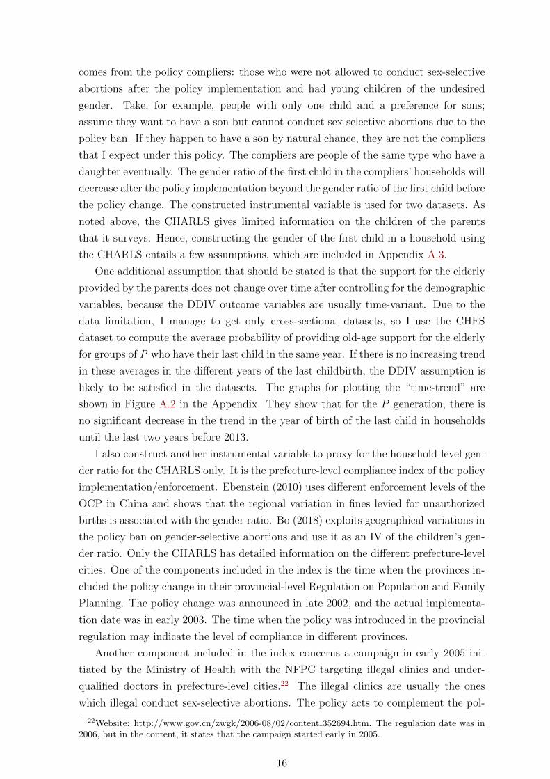
15

comes from the policy compliers: those who were not allowed to conduct sex-selective

abortions after the policy implementation and had young children of the undesired

gender. Take, for example, people with only one child and a preference for sons;

assume they want to have a son but cannot conduct sex-selective abortions due to the

policy ban. If they happen to have a son by natural chance, they are not the compliers

that I expect under this policy. The compliers are people of the same type who have a

daughter eventually. The gender ratio of the first child in the compliers’ households will

decrease after the policy implementation beyond the gender ratio of the first child before

the policy change. The constructed instrumental variable is used for two datasets. As

noted above, the CHARLS gives limited information on the children of the parents

that it surveys. Hence, constructing the gender of the first child in a household using

the CHARLS entails a few assumptions, which are included in Appendix A.3.

One additional assumption that should be stated is that the support for the elderly

provided by the parents does not change over time after controlling for the demographic

variables, because the DDIV outcome variables are usually time-variant. Due to the

data limitation, I manage to get only cross-sectional datasets, so I use the CHFS

dataset to compute the average probability of providing old-age support for the elderly

for groups of P who have their last child in the same year. If there is no increasing trend

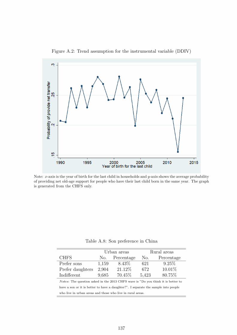
in these averages in the different years of the last childbirth, the DDIV assumption is

likely to be satisfied in the datasets. The graphs for plotting the “time-trend” are

shown in Figure A.2 in the Appendix. They show that for the P generation, there is

no significant decrease in the trend in the year of birth of the last child in households

until the last two years before 2013.

I also construct another instrumental variable to proxy for the household-level gen-

der ratio for the CHARLS only. It is the prefecture-level compliance index of the policy

implementation/enforcement. Ebenstein (2010) uses different enforcement levels of the

OCP in China and shows that the regional variation in fines levied for unauthorized

births is associated with the gender ratio. Bo (2018) exploits geographical variations in

the policy ban on gender-selective abortions and use it as an IV of the children’s gen-

der ratio. Only the CHARLS has detailed information on the different prefecture-level

cities. One of the components included in the index is the time when the provinces in-

cluded the policy change in their provincial-level Regulation on Population and Family

Planning. The policy change was announced in late 2002, and the actual implementa-

tion date was in early 2003. The time when the policy was introduced in the provincial

regulation may indicate the level of compliance in different provinces.

Another component included in the index concerns a campaign in early 2005 ini-

tiated by the Ministry of Health with the NFPC targeting illegal clinics and under-

qualified doctors in prefecture-level cities.22 The illegal clinics are usually the ones

which illegal conduct sex-selective abortions. The policy acts to complement the pol-

22Website: http://www.gov.cn/zwgk/2006-08/02/content 352694.htm. The regulation date was in2006, but in the content, it states that the campaign started early in 2005.

16

icy ban of 2003. Both the central and the provincial governments decide to use this

top-down approach because the local governments may have better control of the ac-

tual implementation of the campaign. Different prefecture-level cities have different

enforcement-level of this campaign. Some cities have mounted this campaign every

year since the campaign started. Others may have implemented the campaign in 2005

for only one year or may even have started the campaign later than the NFPC require-

ment. The number of years that a city has enforced the campaign and also the year

each city started to do so are indicators of the strictness with which the regulation was

implemented at the prefecture-level. I take the relevant information from various pre-

fectural government websites and also from newspapers and generate an index showing

the various compliance levels of the listed prefectural cities regarding this policy and

this campaign. The constructed compliance index varies from 0 to 2, where 2 is the

highest level of allegiance to the aims of the campaign.

The policy implementation levels at the prefectural city-level also link to the choice

of the cluster level in the main regression for the CHARLS. As the policy compliance

level varies in different prefectural cities, it is likely that the residuals for the regressions

for the CHARLS are correlated at the prefecture-level. So, it is reasonable to cluster

the stander error at the prefecture-level for the regression results in the CHARLS. For

the CHFS, because the data does not offer any information on prefectural cities, I

cluster the standard errors at the province-level. The similar argument applies when

using the province-level cluster in the CHFS. The policy enforcement of policies also

varies between different provinces, similar to the OCP enforcement level (Ebenstein,

2010). There is another argument that the error terms should be clustered at the

household-level in generation O in the CHARLS. Under the data reconstruction, some

P and their sibling P are from the same family in O. Also, given the provision of the

old-age support is a household-level decision, the stander errors in the CHFS should

be clustered at the household level. The main results for the CHARLS and the CHFS

are similar to the results in Table A.4 when clustering at different levels. I use the

prefecture-level cluster for the CHARLS and the province-level cluster for the CHFS

for conservative clustered standard errors.

To summarise, the instrumental variables used in the chapter are the gender of the

first child for households having at least one child in or after 2003 and the prefecture-

level compliance index. The IV method exploits three facts: first, that the gender of

the first child is closer to the natural rate than the total gender ratio for all new-borns;

second, that amongst the first-born children, the gender of those who were born in or

after the year of the policy ban is more random; third, that the prefecture-level policy

compliance level is higher when the gender ratio of the children, in general, is lower.

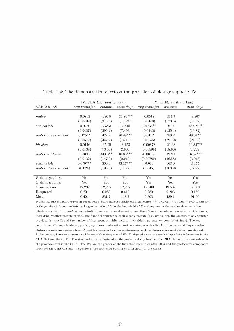
The results from the IV regressions are shown in Tables 1.4. The first stage results are

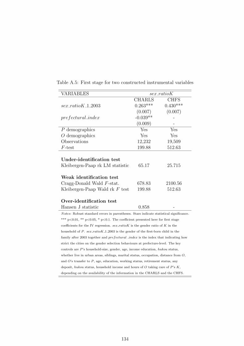
in Table A.5 in the Appendix.

17

1.3.4 Main results

The first three columns of Table 1.4 shows the results for the CHARLS. For any-

transfer, the coefficients of maleP and maleP × hh-size have opposite signs com-

pared to the corresponding coefficients in OLS results, but all four coefficients are

insignificant. The coefficients of maleP and maleP × hh-size for the amount of any

transfers and maleP × hh-size for the visits paid are consistent with the OLS results.

The maleP coefficient for visit days is negative and significant in the IV results. The

CHARLS IV results show that the father demonstration effects are positive for all three

outcomes, and significant for the probability of providing any transfer and the visits

paid. One unit increase in the actual gender ratio of K in fathers’ households increases

the fathers’ probability of providing old-age support to their parents by 7.9%. A simple

interpretation is that, compared to fathers with only daughters, fathers with only sons

are 7.9% more likely to provide support of any support to their own parents. They also

pay 72 days of annual visits more to their own parents. For the mother demonstration

effect, the coefficients of sex ratioK are negative yet insignificant for three outcomes.

These results indicate there might be some potential mother demonstration effects, but

the effects are less significant compared to the father demonstration effects. It implies

that mothers may also try to demonstrate filial piety to their daughters, as the fathers

in the CHARLS do.

The demonstration effect in the CHFS is different from the father demonstration

effect in the CHARLS. The mother demonstration effect is stronger and more signifi-

cant than the father counterpart.23 The coefficients for sex ratioK are negative and

significant for the probability of providing any support and visits paid to their own

parents, and negative for the amount of transfer. Similar interpretations, mothers with

only daughters are 7.3% more likely to provide any support to their own parents than

mothers with only sons. They will also devote 46.9 more days per year visiting their

own parents. In the CHFS, it is difficult to draw any conclusion about the father

effect. The coefficients for sex ratioK + maleP × sex ratioK are insignificant for all

outcomes, and the signs of these coefficients are also inconsistent.

The gender ratio of the third generation is the actual gender ratio of children in P ’s

households. Using the actual gender ratio, I impose a linear assumption on the gender

ratio when interpreting the results. It is possible that the linear interpretation would be

violated when the gender ratio changes from values below 0.5 to values above 0.5. So I

create a variable, more sons, which is a dummy variable equals 1 if the gender ratio is

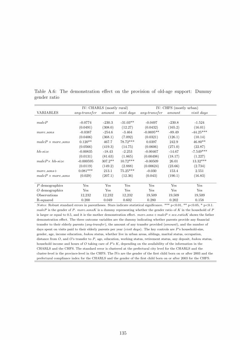
greater or equal to 0.5, and 0 otherwise. The results are presented in Table A.6 in the

Appendix. The coefficients are very similar to and consistent with the ones in Table

1.4. So I continue to use the actual gender ratio sex ratioK as my main regressor in

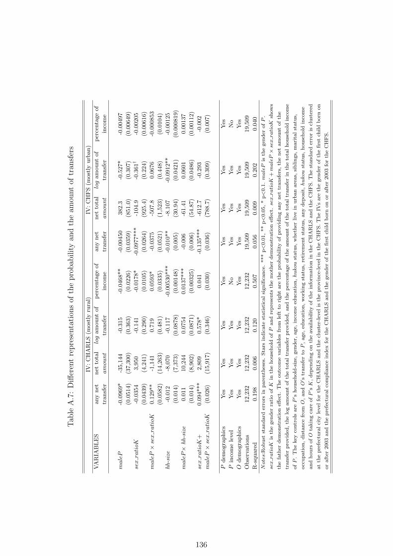
the later analyses. It is also possible the definition of the outcome variables, especially

23The difference between the mother demonstration effects and the father demonstration effect is−2× β − θ, which are significant for the outcomes any-transfer and visit days in the CHFS results.

18

for financial old-age support, could affect the results. In Section A.2 in Appendix A,

I discuss detail about different ways to present the financial old-age support and show

the demonstration effect under the different representations. The signs of the father

or mother demonstration effects in Table A.7 are also mostly consistent with the main

results in Table 1.4, yet the significance-level varies.

The IV results from the CHARLS and the CHFS, they show a very interesting phe-

nomenon. The fathers in the CHARLS and the mothers in the CHFS both demonstrate

to their same-gender children. One possible explanation may be that the CHARLS and

the CHFS focus on different samples. As shown in the summary statistics, one major

difference between the CHARLS and the CHFS is the proportion of urban samples in

each dataset. The CHFS has a sample of which 65.2% live in an urban area, while

the sample in the CHARLS contains 33.2% urban dwellers. In the CHARLS OLS re-

sults, fathers, in general, support their own parents more than mothers do. This result

is consistent with the hypothesis that sons in rural areas are still preferred for their

propensity to provide old-age support. In China’s rural areas, a higher proportion of

people accept traditional gender discrimination/stereotype, and females have less bar-

gaining power in their households than males (Wang and Zhang, 2018). Urban areas

contain more households with a single child than rural areas do as a result of the “1.5”

Child Policy implemented in China (Rosenzweig and Zhang, 2009; Wang and Zhang,

2018).24 If a household only has a daughter, mothers are more likely to demonstrate

to this daughter so that they can look forward to receiving support when they grow

old. Urban areas in China also have more opportunities for female labour market

participants and more gender equality compared to rural areas. My predictions for

the discrepancies between the CHARLS and the CHFS are an urban-rural difference

and/or a single-K/nonsingle-K household difference. The significant female or male

demonstration effect might be driven by the corresponding subsamples with more ob-

servations. The results of a subsample check and heterogeneity analysis provide more

empirical findings on these two conjectures in the following subsections.

There is a possible channel that could also explain the demonstration effects that I

found. Fathers with only or more sons might anticipate receiving more old-age support

in future, thus they are able to provide more old-age support to their own parents

because they do not need to save for their old age. Analogously, it could also happen

to mothers, especially in the urban areas, with daughters as the possible future old-age

support. They could have more money to provide support to their own households.

This channel works in the same directions with the demonstration effect. It is likely

that they co-exist in the real world scenario and also in the empirical results. The key

component that distinguishes the demonstration effect from this possible channel is

that the demonstration behaviours from fathers and mothers need to be observed by

their same-gender children. In the CHARLS, there are two different types of transfer:

24The gender preference in the CHFS is in Table A.8 in the Appendix.

19

regular transfer and non-regular transfer. The regular transfer is the fixed-amount

transfers that parents make to their elderly parents at fixed times, which suits the

definition of old-age support but less visible to their children. The non-regular transfer

represents transfers provided by the parents at festivals, birthdays, weddings, funerals,

and for medical treatments, and also for other non-regular but important social events.

In these family-gathering situations, the provisions of transfer are more visible to their

children. If the channel described and the demonstration effect co-exist, then I would

expect both coefficients representing the father or mother demonstration effects are

significant when using the regular and non-regular transfer as outcome variables. Also,

the magnitudes of these demonstration effects should be larger for the more visible

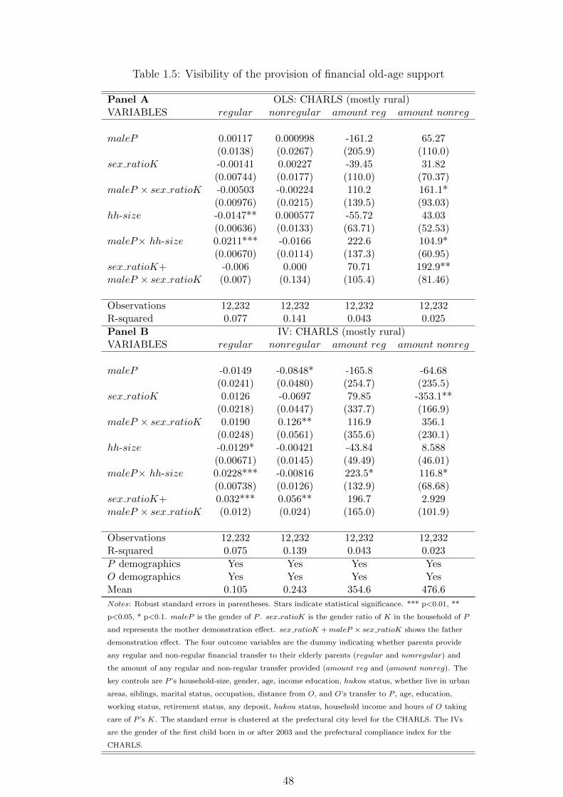
transfer compared to the less visible one.

Table 1.5 show the corresponding results for four different outcomes: the proba-

bility of providing regular and non-regular transfer, and the amount of regular and

non-regular transfer. Focusing on the IV results in Panel B, the father demonstration

effect is 5.6% for the probability of providing non-regular support and 3.2% for the cor-

responding probability for the regular transfer. In terms of the amount of the regular

and non-regular transfer, both father demonstration effects are insignificant. The mag-

nitude of the effect for the regular support is larger than the one for the non-regular.

This can be interpreted as a substitution effect between the regular and the non-regular

support due to household budget constraint. Males are responsible for the regular old-

age support provision, according to the traditional gender norm of the old-age support.

One interesting result from Table 1.5 is the significant mother demonstration effect for

the amount of non-regular transfer. The results suit the traditional norm of old-age

support as provided by adult daughters in rural areas: they are not mainly responsible

for the living expense of their parents. Also, the mother demonstration effects for the

probability of providing non-regular support is positive and insignificant. The results

from Table 1.5 shows that the possible channel discussed could be one of the possible

channels that drives the results, but the larger effects for the probability of providing

more visible old-age support might indicate the demonstration effects also exist.

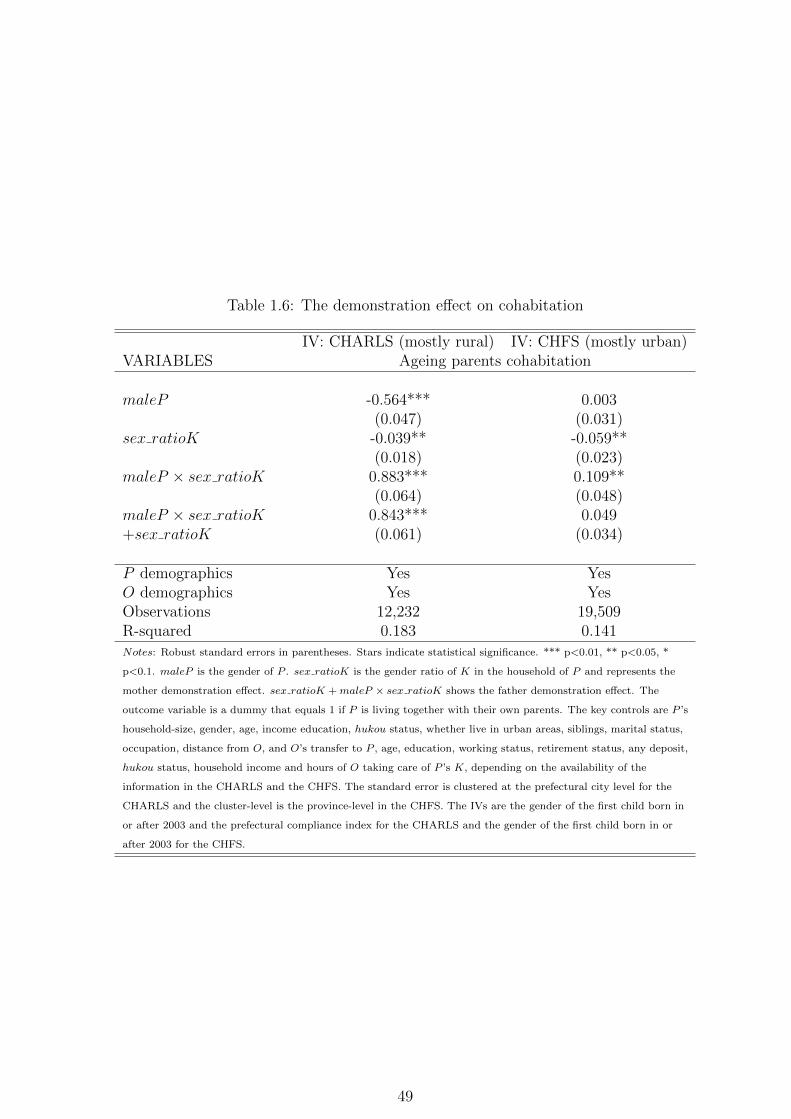
In the main results, I notice the demonstration effects of visits paid to the parents

are larger than other outcome variables when compared to their corresponding mean.

Cohabitation with the elderly parent would be one of the possible explanations for

the large effect in visits paid to O. Living together with the elderly parent is one

important way to take care of them. Although this may count as mutual care of the

family members, it seems that the P generation is more likely to take care of their

elderly parents with respect to income-earning. In the literature, cohabitation with

one’s ageing parents is generally used as an outcome variable. In my specification,

the probability of providing monetary support and the outcome variable visit days

partially capture the cohabitations. I use cohabitations with O as a dummy outcome

variable for both datasets. The prediction of the results would be similar: the same-

20

gender demonstration effects of cohabitation. The results are shown in Table 1.6. Both

mothers and fathers are more likely to cohabit with their own parents to demonstrate

filial piety to their same-gender children, except for the father demonstration effect in

the CHFS results. The father demonstration effects of cohabitation are significantly

larger than the mother effects in the CHARLS. The same-gender demonstration effect

has a higher significant level for this outcome variable than the main CAHRLS results.

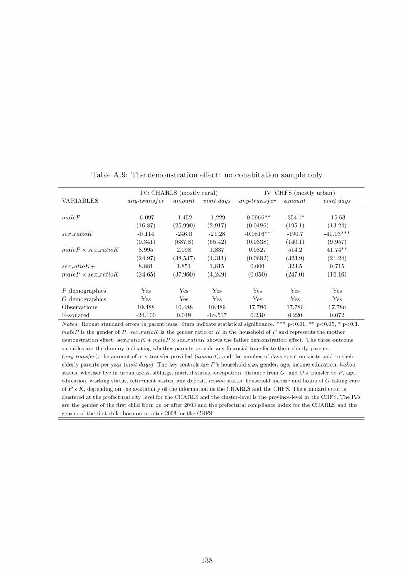
Apart from running the main regression on the cohabitation dummy, I also check

the subsample of those who are not living together with their own parents for their

old-age support provision. The results are in Table A.9. The results imply that the

father demonstration effect in the CHARLS might be fully driven by P who are living

together with their own parents. But in the CHFS, the mother demonstration effect

shows up in the subsample results as well. The living pattern in urban and rural areas

could explain why two subsamples are showing the demonstration effect results for the

CHARLS and the CHFS. Nuclear families are more common in urban areas; while in

rural areas, people are more likely to live with extended family members, especially

with males’ ageing parents and sometimes their male siblings.

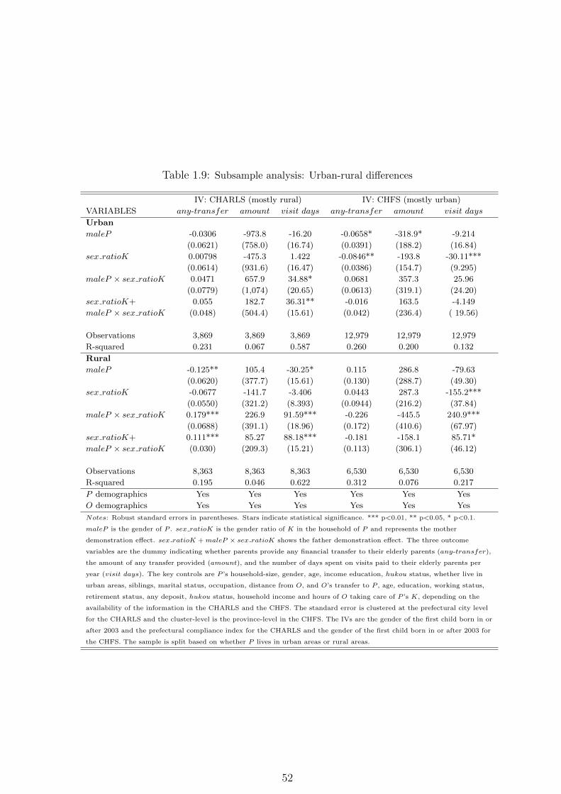
1.3.5 Subsample analysis and heterogeneity check

To verify the effect of the gender composition of K working mostly through the demon-

stration mechanism, I use results from the subsample analysis and the heterogeneity

check to show whether, in different circumstances, the results are still consistent with

the predicted results from this mechanism. The analyses are conducted for both or

only one of the datasets, depending on the available information. I mainly describe

the subsample analysis results and then mention the consistency of the results with

the corresponding heterogeneity checks. Since the CHARLS data exhibits the father

demonstration effect and the CHFS shows the mother effect, I focus only on the fa-

ther effect in different groups from the CHARLS and the mother effect in different

groups from the CHFS. Six categories are used for the analysis: high or low income-

level, singleton or non-singleton households regarding the children, urban or rural res-

idence, parents with or without older brothers, the pension coverage of the parents,

and membership of the Han/non-Han ethnic group. The category for the singleton

or non-singleton households and the urban-rural residence are the two categories that

may provide possible explanations for the discrepancies between the results from the

CHARLS and the CHFS.

Income-level difference

As the future support for the elderly received from the offspring acts as an economic

incentive to have children (Banerjee and Duflo, 2011; Alfano, 2017), households at

different income levels will have different patterns for the demonstration effect. People

in the high-income group will have enough savings, investments, and pension income to

21

support their consumption after retirement. So, their incentive to demonstrate to their

children by pecuniary support for the elderly is not as large as those who in the low-

income group. For the financial old-age support, if the demonstration effect is to obtain

secure private old-age support in future, the subsample results would show larger or

more significant demonstration effects for people in the lower-income group than those

with higher income. Regarding the non-pecuniary support, the high-income group may

demand it as much as or even more than the other group, so larger or more significant

father and mother demonstration effects are also expected for visit days in the high-

income group. The reason for the possible higher demand for non-pecuniary support

for the high-income group is that the time and monetary support are substitutes.

The subsample IV regression results for the CHARLS and the CHFS are shown in

Table 1.7. The CHARLS only have one categorical variable of the household income

level of the parents. To get a balanced subsample in the CHARLS, I classify those whose

household income level above the 20,000 RMB per year category as the high-income

group. The father effects in the low-income group are significant for the two pecuniary

outcomes; while for the high-income, the father demonstration effects are not significant

for these outcomes. For the non-pecuniary outcome, the father demonstration effect

is also significant in both high and low-income group, but the magnitude of the effect

is greater in the high-income group. The mother demonstration effects for visits paid

in the high-income group are positive, yet they are negative in households with a low

income. But both of the mother effects are insignificant. The coefficients seem to be

consistent with the prediction. The evidence for the mother demonstration effect of

pecuniary outcomes is that mother insignificantly signal the old-age support behaviours

to their daughters.

With the detailed income information in the CHFS data, I classify those who have

above the average income in the high-income group and the rest of the sample in the

low-income group. The last three columns of Table 1.7 show that in the low-income

group, mothers increase their visits paid to their own parents with more daughters,

which implies a mother demonstration effect in the non-pecuniary old-age support.

While in the high-income group, the mother demonstration effects are insignificant for

all outcomes. The mother demonstration effect for amount is even positive. For the

insignificant mother effects for visit days, it could be the reason that people in urban

areas with busier lifestyles than rural areas, so people with high income might hire

others to take care of their own parents.

The heterogeneity check provides similar results to those of the subsample analysis.

It can also check whether there are significant differences in the demonstration effect

between the high and low-income groups. The results of the heterogeneity check for

the income-level are shown in Tables A.10 in the Appendix. The CHARLS results

show that the father demonstration effects for pecuniary outcomes are positive and

significant in the low-income group, while they are negative and significant in the high-

22

income group. The differences in the father demonstration effect between these two

subgroups are significant for the two pecuniary outcomes, which indicates the low-

income group has a larger father demonstration effect than the high-income group.

Both groups show positive and significant father effects for the visits paid, yet the

difference is insignificant.

In CHFS heterogeneity results, an important coefficient is the coefficient for sex ratioK

×high income. It is the difference between the mother demonstration effects for P

with high-level income and the mother demonstration effects for P with low-level in-

come, which should be negative and significant if the mother demonstration effects

for P with high-level income are larger than the mother demonstration effects for P

with low-level income. The absolute value of the coefficient of sex ratioK is now the

mother demonstration effect for P with low-level income. The mother demonstration

effect in the high-income group is insignificant for the pecuniary outcomes and positive

and significant for the visits paid. The coefficient for sex ratioK × high income is

positive and significant for the amount of transfer and the visits paid, which implies

the mother demonstration effect for P with low-level income is larger than the effect

for P with high-level income. The CHARLS heterogeneity results are mostly consis-

tent with the subsample analysis, yet the CHFS heterogeneity fit the prediction better

than the subsample results. Both results show the low-income group has larger father

demonstration effects.

The number of the children

This chapter mainly focuses on how the gender of the children affects the support

for the elderly provided by their parents. While the chapter does not, on the whole,

discuss other characteristics of the children, I can use the number of members of the

third generation to conduct a subsample analysis and heterogeneity check. Most of the

households with only one child (‘singleton households’) are the households that strictly

comply with the OCP, even when they have an only daughter. These households may

hold modern views of gender roles; hence, females in these households may be able to

enjoy higher bargaining powers. A preference for sons is a good indicator of whether

a household has more traditional views on gender roles. Such households are more

likely to violate the OCP (or be allowed by “1.5” Child Policy) to have a second child

if their first child is a girl. If the existence of the father and mother demonstration

effects depend on the types of views of gender roles, then I expect larger and more

significant mother demonstration effects in singleton households and father effects in

non-singleton households. Tables 1.8 displays the results for the CHARLS and the

CHFS. The number of children may also correlate with the gender of the first child

in the households, which may lead to biased results in my IV regressions even with

the household size controlled. The subsample analysis of the number of household

children also helps to get rid of the possible bias arising from selections in the number

23

of children for the singleton households sub-group.

The first three columns of Table 1.8 show male P in both types of households in-

crease the visits paid with more sons. P with non-single child family show significant

and positive father demonstration effect in terms of the probability of providing any

transfer to their own parents, while the corresponding father effect is insignificant in

the households with a single child. As discussed in the previous section, given the OCP,

households with more than one child are usually rural households or urban households

with relatively strong son preference. In rural areas, the OCP allows households in

which the first child is a daughter to have a second child, and the law and the enforce-

ment of fines in rural areas are not as strict as they are in urban areas (Ebenstein,

2010). According to Ebenstein (2010), if the OCP is violated in an urban area, the

fine is quite high. Non-singleton households in urban areas usually possess a stronger

preference for sons than singleton ones do; hence, females may have less bargaining

power in non-singleton households. The singleton households in the CHARLS is try-

ing to show up a mother demonstration effect in the pecuniary old-age support, when

the magnitude of the coefficient of sex ratioK is larger in this subsample than the

magnitude in the non-single child households, although both of them are insignificant.

The CHFS results in Table 1.8 show significant mother demonstration effects in sin-

gleton households in terms of the probability of providing any transfers and the visits

paid. But in terms of the amount of provision and the visits paid, the non-singleton

households also show significant mother demonstration effects. The father demonstra-

tion effects are insignificant for both subsamples. The results of the heterogeneity check

for the singleton and non-singleton households are shown in Tables A.11 in the Ap-

pendix. The CHARLS results show that the father demonstration effect in terms of the

visits paid is on average greater in non-singleton households than in singleton house-

holds, yet the difference is insignificant. Table A.11 also shows that in the CHFS the

mother demonstration both exists in the singleton and the non-singleton households.

But, for the amount of transfer provided, the non-singleton group has a larger and

significant mother demonstration effect compared to the singleton group. The hetero-

geneity analysis results are in general consistent with the subsample analysis. Higher

bargaining power for mothers in singleton households is one of my conjectures for ex-

plaining the difference between the CHARLS and the CHFS results. But the CHFS

results do not support this conjecture completely. I need to explain the discrepancy of

the results between the CHARLS and the CHFS by the urban-rural difference.

Urban-rural differences

Another conjecture in explaining the discrepancies between the CHARLS and the

CHFS results is the urban-rural difference. Residences in urban areas in China enjoy

more developed public pension systems, more opportunities for females to be employed

and more gender equality. As the argument in the previous subsample check, with the

24

shift in gender norm of providing old-age support in urban areas, the mother demon-

stration effect should show up more in urban areas, and the father effect should appear

in the rural subsample. Table 1.9 presents the regression results for the urban and ru-

ral subsamples in the CHARLS and the CHFS using the IV regressions. In the urban

and rural areas in the CHARLS, the gender effects of the children are insignificant for

pecuniary and non-pecuniary outcomes of the mother demonstration effect. While in

the rural subsamples, the father demonstration effects are significant for any-transfer

and visit days for the CHARLS. In urban areas, the CHARLS results only show up a

significant father demonstration effect for the visits paid. The heterogeneity analysis

in Table A.12 shows the father demonstration effect for the amount of transfer and the

visits paid is significantly larger in the rural areas. The heterogeneous analysis findings

may indicate that the gender norms as regards support for the elderly are not strong

in urban areas compared to rural areas.

The difference in the gender effects of the children between rural and urban areas in

the CHFS partially corresponds to my prediction. The last three columns of Table 1.9

show that the mother demonstration effect is significant except for amount in the urban

subsample. In the rural subsample, there is no significant demonstration effect for

mothers to their daughters nor fathers to their sons in terms of the pecuniary outcomes.

But the differences between the rural and urban mother demonstration effects are

insignificant. The father demonstration effect for visit days in the rural subsample is

significantly larger than the corresponding coefficients in the urban subsample with

the supporting evidence from Table A.12. This indicates that the gender norm of

providing support for the elderly may still be different between rural and urban areas.

Although the coefficients for the father demonstration effects of the pecuniary outcomes

are insignificant in rural areas in Table 1.9, there may still be gender-role differences

concerning the demonstration effects. The heterogeneity check results in Table A.12

support and are mostly consistent with the subsample analysis results.

The urban-rural subsample analysis partially supports my prediction of more mother

demonstration effects and fewer father effects in urban areas. Scholars believe that fe-

males have higher bargaining power in urban areas in China (Fong, 2002). However,

certain urban households where the first-born is a girl would pay the high fine to have a

son (Ebenstein, 2010). Lee (2012) and Hu and Shi (2018) find that the human capital

investment for boys and girls is not significantly different in singleton households, but

the gap is still wide in multiple-child households. Fong (2002) also limits the rising

female empowerment in urban China only to daughters in singleton households. I run

a simple urban-singleton and other types of household subsample in CHARLS.

I find only significant father demonstration effect in the urban-singleton subsample

is the non-pecuniary outcome. In the non-urban-singleton households in the CHARLS,

the father demonstration effects are again significant for any-transfer and visit days.

The signs of the mother effects are inconsistent between different outcome variables

25

for the urban-single-K subsample, but all negative and insignificant for the non-urban-

singleton subsample in the CHARLS. The CHFS subsample results show significant

mother demonstration effects in the urban-singleton group for any-transfer and visit

days. The results for this simple subsample are shown in Tables A.13 in the Appendix

and are mostly consistent with Table 1.9. The similar results between urban-rural and

urban-singleton subsample results show that the urban-rural difference is a possible

explanation for the discrepancies between the CHARLS and the CHFS results, not only

driven by the urban-singleton households. But both subsample results only provide a

partial explanation for the CHARLS and the CHFS discrepancies, especially for the

outcome any-transfer.

Siblings of the parents

Supporting ageing parents is crucial for most males in China owing to the enduring

cultural impact of Confucianism. Some people have to support their own parents,

regardless of the gender of their children. This is especially true for many males who

provide regular support to their own parents. It may also be the case for some females

in the second generation if they are the oldest child in their own family or have no

older brothers. If people are not fully responsible for the support of their elderly

parents and only want to demonstrate the norm of providing support for the elderly

to their children, the results may show greater effects from the gender ratio of the

children. I use the same regression equations and the identification methods to obtain

the separate results for those who with and without older brothers. The results are

shown in Table 1.10. The CHFS provides only the number of siblings for the main

respondents in households, but no information on his or her rank in the siblings. So

this subsample analysis is conducted in the CHARLS dataset only.

The results indicate that, for the probability of providing any support and also

the visits paid, the father demonstration effects are all significant for those with older

brothers and for those without. The magnitude of all father demonstration effects are

larger in the subgroup for people with older brothers, yet the differences are mostly

insignificant according to the heterogeneity results in Table A.14. Most of the het-

erogeneity results are consistent with the subsample effect, except the father effect is

significantly larger for P without old brother than those who with. The subsample

results suit the predicted results under the demonstration effect channel than the het-

erogeneity analysis results. But I still cannot draw any conclusions on the subsample

check results in this part.

Pension coverage

In the introduction, I treat family support for the elderly as a complement of the public

pension scheme. As Table 1.1 shows, in rural areas where the public pension coverage is

low family-provided support for the elderly is the primary source of support of China’s

26

elderly according to 48% of the NBS survey respondents. Under the demonstration

channel, if parents want to secure future old-age support because they do not have

public pension coverage, then parents without proper pension coverage of their own

are expected to be more likely to provide more support to their own elderly parents

if they have more same-gender children. The demonstration effect will be larger or

more significant for parents without any pension coverage, especially for the pecuniary

old-age support.

To check this hypothesis, I run heterogeneity-analysis regressions on parents with

and without a pension scheme. In the CHARLS, due to the data reconstruction, I

have no information on P ’s pension coverage. However, I can use the occupation

of the parents as a proxy for their pension status. The CHARLS provides six cate-

gories of occupation for the parents, namely, managers; professionals and technicians;

clerks, commercial and service workers; agricultural, forestry, husbandry, and fishery

producers; and production and transportation workers. Of these six categories, the

agricultural, forestry, husbandry, and fishery producers are less likely to be covered by

a pension scheme. I create a dummy, pensionP , that equals 0 if a parent is classified

as an agricultural, forestry, husbandry, or fishery producer, and 1 otherwise. The re-

sults from this heterogeneity analysis are shown in Table 1.11 and they show that the

father demonstration effect is larger for parents if they are less likely to be covered by

a pension system for the visits paid. But for amount, it is the group are more likely to

be covered by a pension showing up the father demonstration effect. Yet the difference

between the father demonstration effects in the group with pension coverage and with-

out is insignificant for the probability of providing any transfer. The empirical results

from the CHARLS only fit part of the description of the relationship between a public

pension scheme and family old-age support. It may due to the pension information is

not detailed enough in the dataset.

In the CHFS, the information is available for defining the exact pension status of the

parents. I create a dummy which equals 1 if a parent is covered by at least one pension

scheme, and 0 otherwise. The heterogeneity check results are shown in the last three

columns of Table 1.11. Yet mothers both with and without any pension coverage have

two out of three negative coefficients corresponding to the mother demonstration effect.

The differences between them show that the mother demonstration effects for P without

any pension coverage are larger the effects in the other sub-group, although only the

difference for amount is significant. The CHFS results in Tables 1.11 might provide a

piece of suggestive evidence on the relationship between public pension schemes and

family support for the elderly suggested previously in the chapter. The conclusion is

difficult to draw from the CHARLS results.

27

Han culture and norm

As discussed in the background section, the norm of providing support for the elderly is

closely linked with Confucianism and filial piety. This raises a possible concern: because

the culture of Confucianism is well-known in Chinese society, not only do parents teach

their children to provide support for the elderly in the future through the demonstration

effect, but also the surrounding community, in schools, the neighbourhood, or the

media, could shape young children’s predilection to provide support to their parents

in their old age. Han ethnic group is the majority ethnic group in China and filial

piety is the key value in the Han group. If other channels apart from the parents

affect children’s preferences regarding old-age support, the demonstration effect from

the parents will be smaller or less significant in a Han-ethnic dominated community or

an exclusively Han-ethnic group.

In the community survey questionnaire in the CHARLS, there is information on

whether minority ethnic groups are living in the same community that the parents live

in. I generate a dummy that equals 1 if there are minority ethnic groups living in the

community, and 0 otherwise. From the results in Table A.15 in the Appendix, the

father demonstration effect for any-transfer and visit days in communities with people

from minority ethnic groups are significant, yet the differences are insignificant for the

fathers in two types of community.

There is no information on the community ethnic composition in the CHFS, but

there is detailed information on P ’s own ethnic groups. So I use this information

to check whether Han ethnic group are more likely to demonstrate the filial piety to

their children than other ethnic groups. I create a Han dummy that equals 1 for

members of the Han ethnic group, and 0 otherwise. In the heterogeneity analysis

results in Table A.16 shown in the Appendix, the mother demonstration effects are

significant for Han ethnic groups in terms of any-transfer and visit days. The effects are

insignificant for non-Han group. Yet, the differences are again insignificant. Combining

the heterogeneity check results from the CHARLS and the CHFS, it seems that there

still are possible mother and father demonstration effects in Han ethnic families and

communities with other ethnic groups, but these effects cannot significantly distinguish

themselves from the corresponding results from the opposite sub-groups.

Migrants and old-age support

The visibility of old-age support is discussed using different types of transfers. The

results seem to show that the demonstration effects are larger when the demonstrative

behaviours are easier for K to observe the demonstration behaviours. When discussing

the visibility of the old-age support, it is also common to focus on the migrants, es-

pecially the rural-to-urban migrants, in China. A lot of migrants work far from their

home town, and a large proportion of them are not living together with their young

children. Given these circumstances, it is difficult for the migrants to signal the norm

28

of providing old-age support to their children. Thus, if the demonstration effects are

the channel driving the results, I would expect the migrant subsample does not show

large and/or significant father and mother demonstration effects.

Neither of the data sets provides very clear information on whether an individual is a

migrant or not. I use a general definition of migrants for both datasets. An individual

is defined as a migrant is one’s hukou status does not match one’s current resident

areas. This means a migrant in this part is people with rural (urban) hukou status

living in urban (rural) areas. I only run the main regressions for the migrant subsample

for the CHARLS and the CHFS. Table A.17 shows the subsample results. The results

show that the migrants in the CHARLS do not show significant father demonstration

effect as the main results in Table 1.3. It implies the visible demonstration effect

could be the right channel explaining the main results for the CHARLS. However, the

results for the CHFS in Table A.17 imply the opposite interpretation. The migrants

in the CHFS show large and significant mother demonstration effects for all three

main outcomes. Female migrants increase the probability of proving any transfer, the

amount of transfers and also visits paid to their own-parents with more daughter in

their own households. The results from CHFS do not seem to support the argument

that the demonstration effect is the channel behind the main results from the CHFS.

Different types of migrants in the CHFS and the CHARLS are one of the possible

explanations for the different results generated from the migrant subsample. 75% of

the migrants in the CHFS have hukou that belongs to the county where their current

residence place. This means that most of them are intra-county migrants, so they can

easily commute between their hometowns and their workplaces. It is relatively easy

for them to demonstrate the norm of old-age support to their children compared to

inter-county or even inter-province migrants. On the contrary, the statistics in the

CHARLS show that 67% of migrants are working in another county or province. The

commuting costs are high for these inter-county or inter-province migrants, so it is less

likely for them to go back to their home town frequently and signal the old-age support

behaviours to their children.

The CHFS also provides information on whether a migrant P lives together with

one’s children and/or own parents. Thus, I further separate the migrant subsample

into two different samples: migrants living with their children but without their par-

ents, and migrants living without their children and parents. The main regressions

run on these two samples, and the results are in Table A.18. The results imply that

females increase the visits paid to their own-parent with more daughters in their own

household for migrants living with their children but without their parents. But this

effect is not significant for migrants living without their children and their parents.

This could suggest that at least part of the mother demonstration effects are signif-

icant in the migrant sample may due to female migrants take their children to visit

their own parents, which makes the provision of non-pecuniary old-age support more

29

visible to their children. Other mother demonstration effects for the financial support

are similar in these two different migrant subsamples, which, again, the intra-county

migrant behaviour is one of the possible explanation for the significant effects.

1.4 Robustness check

1.4.1 Mechanism check

There are other different channels that may explain the effects of children on the

support for the elderly provided by their parents. Testing the subsamples may show

what are the main drivers behind the effects of children’s gender on the parents’ support

for the elderly provision. In this section, I also check other mechanisms discussed in the

literature review section and try to disentangle the demonstration effects from other

possible mechanisms. I first discuss the channels of altruism and direct reciprocity

that may affect my empirical results and go on to discuss the effectiveness of the

demonstration effect.

Education investment in K

The difference in the education investment in the children could be one of the possible

explanations for the mother demonstration effect. The significant mother demonstra-

tion effect in the CHFS may result from the fact that mothers with daughters are less

likely to invest in their daughters’ human-capital such that they can provide more for

their parents. However, this argument does not work for the father demonstration

effects because human capital investments in sons in China are on average higher than

the investments in daughters, except for urban singleton households (Fong, 2002). In

addition, I run the main regressions on three new outcome variables that indicate the

education investment for K.

Only the CHFS offers information on the education investments in K. The evidence

from the CHFS is shown in Table A.19. It shows that, at least in the CHFS, mothers

with more daughters increase the amount of education investment and the percentage

of education investment in the household expenditure, and decrease the probability

of investing in K’s education, controlling for the household size. For fathers with the

household size fixed, with more sons, they increase the probability of investing in K’s

education and decrease the amount of education investment and the percentage of

education investment in the household expenditure. From the results, the gender of

K affects the total amount of education investment and the probability of providing

education investment in different ways, so I cannot draw the conclusion on whether

mothers and fathers invest more on their daughters or their sons. So the possibility of

the different education costs in sons and daughters of P might not be the main channel

working for the mother demonstration effect found in the CHFS results.

30

Altruism and Direct reciprocity channel

The first possible mechanism is altruism. If the main mechanism is pure altruism,

the only reason behind the parents providing support to their own elderly parents is

that these parents are poor and in need of help. There should not be any significant

coefficients for the gender of the adult children, the gender ratio of the children or

their interaction term after controlling for the income of the elderly parents in the

regression. I run heterogeneity checks on the elderly parents’ income-level as included

in the CHARLS. In the sample, most of the elderly parents observed have no income, so

I create a dummy income of O which equals 1 if the elderly parents have some income,

and 0 otherwise. The results are shown in Table 1.12. They reveal that, for any-transfer

and visit days, the father effect is significant for elderly parents without any income,

whereas for the high-income group, the effects are positive but insignificant except for

the father effect for visit days. However, the key is that the difference between these

two groups is also insignificant. I may draw the conclusion that there is a certain degree

of altruism among the motives of providing support to one’s elderly parents, but it is

not the main channel working behind the empirical results in this chapter.

Another mechanism discussed in the previous section is direct reciprocity. One

kind of direct reciprocities in the context of old-age support is the parents’ desire to

support ageing parents to repay the investment in their childhood. I name this kind

of direct reciprocity as sequential direct reciprocity. It may also explain why females

provide less support to the elderly to their parents because, according to the CHARLS,

they did not get enough financial or non-financial investment from their parents during

their childhood. Only the CHARLS includes this type of information, so I use only

this dataset to check this mechanism.

If sequential direct reciprocity is the only channel for old-age support to flow along,

then controlling in the regression for the same financial and non-financial investment

received by the parents in their childhood should confirm that males and females in

the P generation should provide the same amount of old-age support. Moreover, the

gender of the children should not have different effects on the transfers provided by the

parents. I control for different variables that indicate the financial investment and non-

financial investment the P received during their childhood in the regression. The results

are shown in Table 1.13. There are two variables represent the time investment (non-

financial support) during the parents’ childhood. awaytime is the variable representing

how long a P has been away from his or her parents in childhood, and awayage indicates

the age when the parent left her/his parents.

The log edu expense indicates the financial investment in education that P received

in their childhood. I also show the coefficients for edu level in the table, which is the

education level controlled in the main regression. It is another indicator of the size of

the financial investment. Table 1.13 shows that, after controlling for the non-financial,

financial investment, and their interaction terms with maleP , the coefficients that

31

represent the demonstration effect are still similar to the results in Table 1.4. With most

of the coefficients representing the father demonstration effect being still significant,

it also suggests that the same-gender demonstration effect also works as one of the

potential channels. Most of the coefficients including awaytime, awayage, log edu

expense, edu level, and their interaction terms with maleP are insignificant as well.

In addition to the results in Table 1.13, the CHFS main results may also demonstrate

that this sequential direct reciprocity channel is not the main mechanism. In general,

mothers provide more to their own parents in the CHFS than fathers, given the fact

that females on average have a lower education level than males.

Another direct reciprocity channel works through the transfers from the elderly

parents to the parents in the same period. This is a type of non-sequential direct

reciprocity. In the previous regressions in the CHARLS and the CHFS, I control the

transfer from the elderly parents to the parents. This variable would, in theory, have

positive effects on the outcome variable, and vice versa. I also control for the time

that the elderly parents spend on taking care of the children of the parents and also

the transfer to the children in the regressions in the CHARLS. For the robustness

check, I show the regression results without these controls in Table A.20, also their

corresponding coefficients in Table A.21. The key results are similar to the main

results, except for the mother demonstration effect for any-transfer in the CHFS. The

coefficients for these transfers exhibit positive father and mother demonstration effects

on the transfers provided.

The rationale behind the non-sequential direct reciprocity is that if the parents

with more same-gender children receive more from their elderly parents than those

receiving less, then they also provide more old-age support. However, when I run

the same regression on the transfer received by the parents from their elderly parents,

the CHARLS results appearing in the second column of Table 1.14 show that people

who provide more to their elderly parents, namely fathers with more sons, receive less.

Also, for the CHFS in the fourth and the fifth column of Table 1.14 show the fathers,

who are more likely to receive transfers from their parents with more sons, are not

more likely to provide transfer to their parents. Also, in the CHFS, mothers increase

the probability of old-age support provision with more daughters but are less likely

to receive transfers from O. The results may fit the explanation by Li et al. (2010):

the elderly parents may show more altruism toward their adult children, which are P ,

who do not provide more transfer than others, rather than expecting commensurate

paybacks from the parents who receive their support. To conclude, the non-sequential

direct reciprocity may exist, but there is still room for the proposed mechanism: the

demonstration effect.

The CHARLS results in Table A.21 show that the coefficients for both time and

financial transfer from elderly parents to their grandchildren are positive for most of

the outcome variables. This may suggest another form of indirect reciprocity. The

32

elderly can transfer to their favourite grandchildren. If the favourite grandchildren

receive more, their parents (the parent generation) are more likely to provide support

to the ageing parents, O, in return. This type of indirect reciprocity has no time lag

for the payback, unlike the demonstration effect studied in the present paper. Usually,

the preferred grandchildren are grandsons. This could be one of the explanations of

the father demonstration effect in the CHARLS. If the indirect reciprocity works in

this way, male parents with more sons should have more transfers from their elderly

parents to their sons. However, the third column of Table 1.14 shows that, statistically,

male P ’s sons do not receive more than daughters of males with more daughters. These

grandchildren gender effects are not significant for transfers from elderly parents. Thus,

it is less likely to be the main channel driving the main results observed.

Effectiveness of the demonstration effect

Apart from verifying the possible channels, I also have to test for the effectiveness of

the demonstration effect in the datasets. The parents expect their children to provide

support to them in the future. The previous results imply only that the parents

demonstrate filial piety to their children, but they do not show whether the children

actually go on to provide old-age support to their parents in the future. Using the

CHARLS dataset only, I obtain the information on support in old age that is provided

by the elderly generation to their own parents, who are the grandparents of the parent

generation. I run a simple OLS regression to regress the upward-transfers of males and

females among the elderly parents to their own parents on the outcome variables used

for the CHARLS results. I run the regression separately for male and female parents.

The types of transfer provided by the elderly parents to their own parents on the left-

hand side of the equation also match the corresponding dependent variables. Take,

for example, the regressions for log(regular), two key regressors, father’s transfer and

mother’s transfer, these are the logarithm amount of the regular transfer provided by

the father and mother of the present parents’ generation to their own parents in an

earlier sequence. The outcome variables are the probability of providing any, regular,

and non-regular transfer, and the logarithm of the amount of regular and non-regular

transfer. The control variables are the same as the controls in Table 1.2. One extra

control that I have for the particular regressions is the average self-reported health of

the grandparents of the parents. The health problems of P ’s grandparents may affect

the support provided.

To simplify the description of the results, I continue to use the O, P , and K setting

in this part. The results are combined in Table 1.15. The key regressors for male and

female P panels are father’s transfer and mother’s transfer. For male and female P ,

the demonstration effects seem to take into account the effects from the same gender

channel: females are more affected by the support for the elderly provided by their

mothers than their fathers’. The converse is partially true for males. The same-gender

33

demonstration effect is more significant for female members of P than the cross-gender

demonstration effect. The magnitude and also the significance level for father’s transfer

are much smaller than the mother’s transfer for female P ; while for males P , the

difference is not large. The results show that if the members of O provide more to

their parents, they are more likely to receive more from P .

1.4.2 Panel results: Event study

The main regression results mainly show the cross-sectional empirical evidence of the

demonstration effect. The conclusion will be more convincing if there is empirical

evidence from a panel dataset. Both the CHARLS and the CHFS are longitudinal

datasets, but CHARLS does not provide information on the gender composition of

the children for the whole sample in the 2013 and 2015 wave. The CHFS contains

this necessary information in the 2011, 2013, and 2015 wave. The reason for using

this three-wave dataset is to gain more yearly data before and after the event. The

drawback of using the CHFS is that I can only test the demonstration effect on one

consistent outcome variable - the probability of providing old-age support - for three

different waves. Together with the limited number of waves in the CHFS, I use only

the panel result as a robustness check for the main results.

To examine the yearly effect of having a son or a daughter on old-age support, I use

the event study approach. The event is the birth of the first child. The event usually

causes sharp changes in several outcomes for the parents, especially labour market

outcomes (Kleven et al., 2018). I apply a similar event study approach to that used by

Kleven et al. (2018) and aim to show even possible causal results in the event study

approach. In the three-wave panel dataset, the sample is still limited to household

respondents. Given the event study approach setting and the limited number of waves

for the data, the panel sample includes only those respondents whose first child was

born between 2011 and 2015. For each household respondent, I set the event time

e = 0 for the year in which the respondent has his or her first child. The value of other

years is set relative to the e = 0 year. Using the specification in Kleven et al. (2018),

the regression is:

yite =∑j

αj × I[j = e] +∑k

βk × I[k = ageit] +∑l

γl × I[l = t] + εite, (1.2)

where i stands for individual i, t for wave t, and e for the event time e. yite is the

probability of providing support to elderly parents. I[j = e] represents the event time

dummies, I[k = ageit] is for the age dummies, and I[l = t] is the wave fixed effects. By

controlling the age dummies, I can control the non-parametrical underlying life-cycle

trend (Kleven et al., 2018). I run this regression separately for four different groups:

fathers with a first son (father-son), fathers with a first daughter (father-daughter),

34

mothers with a first son (mother-son), and mothers with a first daughter (mother-

daughter). Then I compare the results for the parents within a certain gender and

observe that the effect of having a first son/daughter on the father/the mother. The

reason why the results may be causal is that I examine the variation in the results

caused by the gender of the first child. As noted in the previous section, the gender

of the first child is almost exogenous. In addition, the timing of the birth for the first

child is after 2003, which is after the ban on the use of ultrasonography techniques for

sex-detective abortions. The regression results are shown in Table 1.16. The sample

size for each group is around 800 observations, which also indicates that the gender of

the first child in the event study sample is satisfactorily balanced.

The graph for the plot of the event time dummies coefficients is shown in Figure

1.5. The graph on the left shows the difference between fathers with a first son and

fathers with a first daughter. The right graph is the difference between mothers. After

the birth of a first child, the mothers with a first daughter provide more than those

with sons, whereas the differences between fathers are relatively small. For the pre-

trend of the event study, I can only observe one period before the birth of the first

child in the panel dataset due to the limitations of the data. But from this one-period

pre-trend result, it seems that for mothers and father, the pre-trend differences are

insignificant. Lack of the pre-trend time period will affect the validity of the inference

and the causality of the event study results. But the results may provide some insights

into the effects of the gender of the children on the old-age support provided by their

same-gender parents.

There is a concern that the mother demonstration effect from the event study takes

off from the birth year of the child. For the demonstration effect, K have to observe the

corresponding behaviour of their same-gender P . More likely to provide old-age support

during the very early stage of K’s life (age 0-2) would not help with the interpretation

of the demonstration effect. However, the birth of a new child is a big change in

household composition. According to Heath and Tan (2018), “a daughter raises her

mother’s participation in household decisions”, and the mothers with daughters would

seek more female autonomy in their households. With a newborn girl in the family,

it is likely that the mother realises that she needs to start to participate more in the

decisions on the household resources allocation and to provide more old-age support to

her own parents, so she could affect her daughters’ norm formation later and receive

more old-age support in her old age.

It is also possible that a mother with a newborn daughter will receive more support

from her own parents. However, the transfers from the elderly are not included in the

construction of the outcome variables used in the main regressions. I change the transfer

outcome variables to net transfer variables. If any-transfer, regular or nonregular

equals 1 and the parents receive the transfers from or are living together with their

elderly parents, I change the corresponding value to 0. For the amount of transfer, I

35

use the net transfer provided by the parents, which is the amount of transfer provided

to the parents minus the amount of the transfer received by them from their elderly

parents. The change is made for both datasets. The results for the net transfers are

shown in Table A.7. They are consistent with the main results, except for the negative

father demonstration effect for any-transfer in the CHFS. The magnitudes of the

demonstration effect also increase beyond the main results.

1.5 Welfare analysis

1.5.1 “Missing women” and the old-age support

As pointed out by Qian (2008), the future income of children will affect their gender

ratio, and parents expect in their old age to receive support from their children . My

empirical results show the causality of the support for the elderly provided by the par-

ents and the gender of their children. It may be possible to draw some inferences on

the correlations between the support for the elderly and the gender of children from

the literature and my results. The results in the chapter show that, in rural areas,

males provide more in general, and the effects are more persistent for households with

consistent male heirs over several generations. I may be able to argue that support for

the elderly is at least correlated with the gender ratio, or the “missing women” in China

may be correlated with the demand for support in old age. I follow Oster’s method in

2005. She calculates the number of “missing women” in China due to hepatitis B infec-

tion. She estimates the effect of prevalent hepatitis B on the male-female gender ratio

and calculates the hepatitis B-adjusted gender ratio using the percentage of the pop-

ulation infected with hepatitis B. She draws the conclusion that hepatitis B accounts

for 75% of the “missing women” in China. Her results are not entirely accurate due to

the data that she collected, but her method provides a reasonable estimation strategy

to evaluate how much the unbalanced gender ratio can be correlated with hepatitis B

infection. I use her method of estimation to measure the possible correlation between

the “missing women” and the need for support in old age.

I use the CHFS to conduct the estimation.25 One of the advantages of using the

CHFS is that the dataset provides people’s attitudes on family, children and support for

the elderly. There are two relevant questions in the survey: “Do you prefer daughters

or sons?” and “Who do you think is responsible for your care in old age?”. I created

a dummy that equals 1 if people prefer sons and believe that their children should be

responsible for supporting their elderly parents and 0 otherwise. I obtain the mean of

this dummy in the full sample in the main regressions, the urban subsample and rural

subsample. Running the dummy on the gender ratio of the children, the coefficient

for the dummy, which is the prevalence of old-age support, is shown in the second

25The CHARLS does not contain many questions on people’s ideology, so I cannot distinguish thosewho have a preference for sons from whose who do not.

36

column of Table 1.17. Then I calculate the estimated gender ratio on the sole basis

of the prevalence of support for the elderly shown in the third column. Given that

the natural male-to-female gender ratio (1.049) and the percentage of people who

prefer sons and who believe that their children should be responsible for their old-

age support, I calculate the adjusted gender ratio in Column 5.26 The equation for

the adjusted gender ratio is GRadjust = GRold−age× percentageold−age +GRnonold−age×(1 − percentageold−age) (Oster, 2005). The percentage of the gender ratio correlated

with the needs of the future support for the elderly is listed in the last column. From

the estimations, around 12%-18% of the unbalanced gender ratio is correlated with the

needs for support in old age. 17.23 million Chinese babies were born in 2017, and the

medium gender ratio for 2015-2017 is 1.150 according to the world population prospects

in 2017.27 If people conduct gender selections to secure future support in their old age,

the number of “missing girls” due to this would have been around 93,000 in 2017.

1.6 Conclusions

The existence of a younger generation plays an essential role in parents’ decisions on

the support that they provide for the elderly. This chapter finds that the gender of the

children in China affects the support for the elderly provided by their parents. The

parents are more likely to provide more financial and non-financial support to their

ageing parents when they themselves have more same-gender offspring, which is the

demonstration effect. However, the demonstration effects by mothers and fathers are

exhibited in different areas in China. Rural areas show the father demonstration effects

while mother demonstration effects appear in urban areas. The urban-rural difference

may be due to female empowerment in urban areas, but this needs to be verified by

future studies. The demonstration effect is a way for the norm of providing support

in old age to be conveyed to future generations. The intergenerational transmission of

norms is also gender-specific.

This chapter predicts that support for the elderly provided by a father increases

when more sons in his family and when he has greater bargaining power than his wife,

fixing his household size constant. The support for the elderly provided by mothers

increases with the advent of more daughters and when mothers earn more income. The

empirical results of the gender ratio for the household’s children match the predictions

of the model in the next chapter. In China, urban females have more bargaining

power in their households than females in rural areas have. The findings indicate

that the mother demonstration effect mainly shows up in the dataset with more urban

26The percentage of people who prefer daughters or who have no preference, and who believe thattheir children should be responsible for their support in old age is 34.38% for the full sample, 47.48%for the rural subsample and 18.39% for the urban subsample.

27The source for these data can be accessed through the following web-sites: https://www.statista.com/statistics/250650/numberof-births-in-china andhttp://data.un.org/Data.aspx?d=PopDiv& f=variableID%3A52.

37

samples. The heterogeneity analysis for the urban households further suggests that the

assumption of intra-household bargaining is valid. The theoretical model that support

the empirical results is in Chapter 2.

The empirical evidence shows that the gender of the parents and their children in

China jointly affect the likelihood and the amount of old-age support, both financial and

non-financial, that they provide. The story behind this is more complicated than any

pure gender effect from the children. The proposed mechanism, with the same-gender

intergenerational transmission, is indirect reciprocity, or the demonstration effect. It

carries the social norm of providing private support for the elderly across the genera-

tions. Given the heavy financial burden of the public pension system facing the central

government in China, the government has realised that private support for the elderly

is a crucial complement to the public pension. In 2017, the central government started

a pilot implementation of “homebased old-age care services”. One of the expected

goals of this pilot implementation is to collect information on the demographics of all

households with ageing parents and use the information to set future policies or in-

centives for completing the home-based system of care services for old people.28 The

empirical results in the present paper can offer some insights into the demographics of

those who provide or do not provide support to their ageing parents: policy-makers

could introduce diverse incentives in order to target different groups. The rural-urban

discrepancies in the results will also help the government to set targeted policies in

rural and urban areas.

Although the Chinese government has become aware of the importance of private

support for the elderly and has started to promote “filial piety”, there may be a hidden

hazard behind this action. As this chapter shows, sons in rural areas in China provide

more support for the elderly than daughters do. The previous literature also states that

economic incentives, especially old-age support, provide one reason for sex selection

before birth (Qian, 2008; Ebenstein and Leung, 2010). The gender ratio might stagnate

at a high level, to create a damaging equilibrium. The government needs to promote

gender equality by legislating to protect the right of females to inherit, own property

and compete in the labour market, especially in rural areas. In urban areas, there is

already a healthier balance in the gender ratio of new-borns. Mother demonstration

effects showing in urban areas alone may also be due to female empowerment and

higher bargaining powers in the household for females. More research is needed to

confirm this possible mechanism.

28Website: http://xinhuanet.com/gongyi/yanglao/2017-04/17/c 129543350.htm

38

1.7 Figures and Tables

39

Figure 1.1: Public service announcement posters in China

40

Figure 1.2: Actual gender ratios for the newborns in China: the yearly trend

Note: The information is obtained from the China Population and Employment Statistics Yearbook.1982-2011. y-axis is the male to female gender ratio for the newborns (female=100). x-axis is the year1982 to 2011. The yearly trend started in 1987. The circle dot is the national male to female genderratio. The diamond dot represents the male to female gender ratio in urban areas only. The triangleand square dots are for the male to female gender ratio in township (suburban) areas and rural areasrespectively.

41

Figure 1.3: Estimated gender ratios for the newborns in China: the yearly trend

Note The graphs are the estimated male-to-female gender ratio for the newborns in China using the2011 CHARLS wave (above), and the estimated male-to-female gender ratio for the first-born childin the 2013 CHFS wave (below). y-axis is the male-to-female gender ratio (male newborns divided bythe total number of newborns). x-axis is the year from 1995 to 2011 for the CHARLS and from 1995to 2013 for the CHFS. The dots represent the estimated gender ratio for each year. The red verticalline represents the implementation of the policy ban on gender-selective abortion. The solid line isthe linear estimation of the gender ratio trend before 2003, and the dashed line is the estimated lineartrend after 2003.

42

Figure 1.4: Actual gender ratios for the newborns in China: by birth order

Note: The information is obtained from the National Population Census. 1990, 1995, 2000, 2005 and2010. The figure shows four graphs on the male-to-female gender ratio (female=100) of the new-bornsby different birth orders. From left to right, the graphs show the gender ratios in China, urban areas,township (suburban) areas, and rural areas. The circle dot is the overall gender ratio. The diamonddot represents the ratio for the first-born children. The triangle and square dots are for the male tofemale gender for the second-born and the third-born children respectively.

Figure 1.5: Impact of the gender of the first child on the probability of providing anyold-age support

Note: The graphs are the plot of the coefficients in Table 1.16. y-axis is the probability of providingany transfer to O, and x-axis is the event time. The event is the birth of the first child in households.The graph on the left is the coefficients for males and the right graph is the results for females. Thediamond dot coefficients represent people with first child as a son. The square dot coefficients are forpeople with first child as a daughter. Due to data limitation, I can only get one period before theevent in the panel dataset.

43

Table 1.1: Primary source of support of China’s elderly, 2005 and 2010

2005

Urban RuralSource of support Average Male Female Average Male Female

Labour income 13.0 18.4 7.9 37.9 48.5 27.5Pensions 45.4 56.9 34.6 4.60 8.1 1.3Dibao 2.4 1.8 2.9 1.3 1.8 0.9

Insurnace and subsidy 0.3 0.3 0.2 0.1 0.2 0.0Property income 0.5 0.5 0.5 0.2 0.2 0.1Family support 37.0 20.7 52.3 54.1 39.3 68.5

Other 1.5 1.4 1.6 1.8 2.0 1.7Source: NBS, 2006. Most significant share of support reported.

2010

Urban RuralSource of support Average Male Female Average Male Female

Labour income 6.16 9.72 3.75 41.18 50.53 32.14Pensions 66.30 74.21 58.99 4.60 7.19 2.09Dibao 2.33 1.76 2.87 4.48 5.14 3.85

Insurnace and subsidy - - - - - -Property income 0.68 0.75 0.62 0.19 0.21 0.16Family support 22.43 12.13 31.95 47.74 35.13 59.93

Other 1.64 1.44 1.83 1.81 1.79 1.83Source: NBS, 2011. Most significant share of support reported.

44

Tab

le1.

2:Sum

mar

yst

atis

tics

:K

eyva

riab

les

CH

AR

LS

CH

FS

VA

RIA

BL

ES

Mea

nS

td.

Dev

.M

inM

axM

ean

Std

.D

ev.

Min

Max

wh

eth

erP

pro

vid

esan

ytr

an

sfer

s0.2

840.

306

01

0.265

0.441

01

regu

lar

tran

sfer

0.1

050.

272

01

--

--

non

-reg

ula

rtr

ansf

er0.2

430.

308

01

--

--

amou

nt

ofto

tal

tran

sfer

831.

245

98.6

010

0000

599.

216

49.8

010

,000

regu

lar

tran

sfer

354

.638

73.1

010

0,00

0-

--

-n

on

-reg

ula

rtr

ansf

er476

.630

65.6

010

0,00

0-

--

-vis

itd

ays

118.

72.

374

036

591

.66

145.

40

365

gen

der

ofP

0.5

130.

500

01

0.499

0.500

01

gen

der

rati

oofK

0.5

620.

405

01

0.567

0.416

01

hou

seh

old

size

ofP

3.6

430.

774

210

3.662

0.889

211

age

ofP

39.

739.

287

2165

48.1

710.

71

21

65in

com

ele

vel

ofP

5.0

781.

420

111

--

--

inco

me

ofP

--

--

21779

436

390

164

9439

edu

cati

on

ofP

0.8

920.

496

02

0.832

0.646

02

wh

eth

erP

has

aru

ralhukou

0.6

800.

466

01

0.546

0.498

01

Pli

vin

gin

rura

lar

eas

0.65

20.

476

01

0.33

20.4

71

01

No.

of

sib

lin

gsofP

3.7

581.

612

110

3.218

1.856

016

mar

ital

stat

us

ofP

0.9

980.

040

01

0.763

0.425

01

pro

fess

ion

al

titl

e/occ

up

atio

nofP

0.1

050.

547

04

0.902

1.717

08

any

tran

sfer

sfr

omO

0.0

370.

190

01

0.144

0.351

01

aver

age

edu

cati

onle

vel

ofO

2.8

981.

665

19.

51.

894

1.104

07

P’s

ran

kin

gin

sib

lin

gs2.

391

1.39

61

10-

--

-w

orkin

gst

atu

sofP

--

--

0.68

80.4

63

01

dis

tan

cefr

omO

3.2

651.

837

07

--

--

gen

der

ofh

ou

seh

old

hea

dofO

0.43

90.

496

01

--

--

aver

age

age

ofO

63.9

410

.441

4210

1-

--

No.

ofO

aliv

e-

--

-1.

230

0.9

29

02

aver

age

work

ing

stat

us

ofO

0.56

80.

453

01

--

--

aver

age

pen

sion

ofO

0.18

50.

388

01

--

--

wh

osh

ould

sup

por

tO

1.62

61.

042

15

--

--

hav

eO

reti

red

1.8

750.

301

12

--

--

wh

eth

erO

are

part

ym

emb

ers

--

--

2.086

0.929

10

3w

het

herO

hav

ed

epos

it0.

137

0.34

70

1-

--

-hukou

stat

us

ofO

--

--

2.08

60.9

291

03

hou

seh

old

inco

me

ofO

1576

6143

3635

90

2.00

e+8

--

--

hou

rsofO

takin

gca

reofK

530.

901

1816

.50

1713

6-

--

-

45

Table 1.3: The demonstration effect on the provision of old-age support: OLS

OLS: CHARLS (mostly rural) OLS: CHFS(mostly urban)

VARIABLES any-transfer amount visit days any-transfer amount visit days

maleP 0.0104 -95.90 14.51*** -0.0325** -99.75 23.70***

(0.0281) (233.8) (5.201) (0.0153) (63.95) (6.275)

sex ratioK 0.00471 -7.627 -4.680** -0.0119 -38.61 -1.326

(0.0172) (136.6) (2.352) (0.00968) (51.97) (3.441)

maleP × sex ratioK -0.0108 271.2 10.39*** 0.00977 41.14 6.089

(0.0215) (175.7) (3.853) (0.0116) (62.96) (5.324)

hh-size -0.00910 -12.69 -4.398** -0.00527 -20.49 -7.979***

(0.0129) (89.94) (1.829) (0.00527) (18.53) (1.263)

maleP× hh-size -0.000565 327.5** 12.22*** -0.00299 30.36 14.73***

(0.0120) (152.5) (2.837) (0.00675) (24.30) (2.843)

sex ratioK+ -0.006 263.6* 5.713* -0.002 2.535 4.762

maleP × sex ratioK (0.013) (142.8) (3.251) (0.009) (38.86) (4.208)

P demographics Yes Yes Yes Yes Yes Yes

O demographics Yes Yes Yes Yes Yes Yes

Observations 12,232 12,232 12,232 19,509 19,509 19,509

R-squared 0.205 0.050 0.628 0.282 0.203 0.168

Mean 0.401 831.2 118.7 0.303 489.1 91.66

Notes: Robust standard errors in parentheses. Stars indicate statistical significance. *** p<0.01, ** p<0.05, * p<0.1. maleP

is the gender of P . sex ratioK is the gender ratio of K in the household of P and represents the mother demonstration

effect. sex ratioK +maleP × sex ratioK shows the father demonstration effect. The three outcome variables are the dummy

indicating whether parents provide any financial transfer to their elderly parents (any-transfer), the amount of any transfer

provided (amount), and the number of days spent on visits paid to their elderly parents per year (visit days). The key

controls are P ’s household-size, gender, age, income education, hukou status, whether live in urban areas, siblings, marital

status, occupation, distance from O, and O’s transfer to P , age, education, working status, retirement status, any deposit,

hukou status, household income and hours of O taking care of P ’s K, depending on the availability of the information in the

CHARLS and the CHFS. The standard error is clustered at the prefectural city level for the CHARLS and the cluster-level is

the province-level in the CHFS.

46

Table 1.4: The demonstration effect on the provision of old-age support: IV

IV: CHARLS (mostly rural) IV: CHFS(mostly urban)

VARIABLES any-transfer amount visit days any-transfer amount visit days

maleP -0.0802 -230.5 -29.89*** -0.0518 -237.7 -3.363

(0.0499) (316.5) (11.24) (0.0448) (173.5) (16.57)

sex ratioK -0.0450 -273.3 -4.315 -0.0733** -96.20 -46.92***

(0.0437) (399.4) (7.493) (0.0343) (135.4) (10.82)

maleP × sex ratioK 0.125** 472.9 76.49*** 0.0412 259.2 49.37**

(0.0579) (442.2) (14.13) (0.0645) (291.9) (24.53)

hh-size -0.0116 -35.25 -3.153 -0.00878 -21.63 -10.35***

(0.0139) (73.55) (2.005) (0.00599) (18.06) (1.259)

maleP× hh-size 0.0085 340.3** 16.66*** -0.00180 39.99 16.52***

(0.0132) (147.0) (2.910) (0.00789) (26.58) (3.048)

sex ratioK+ 0.079*** 200.0 72.17*** -0.032 163.0 2.455

maleP × sex ratioK (0.026) (190.6) (11.72) (0.045) (203.9) (17.92)

P demographics Yes Yes Yes Yes Yes Yes

O demographics Yes Yes Yes Yes Yes Yes

Observations 12,232 12,232 12,232 19,509 19,509 19,509

R-squared 0.201 0.050 0.610 0.280 0.203 0.159

Mean 0.401 831.2 118.7 0.303 489.1 91.66

Notes: Robust standard errors in parentheses. Stars indicate statistical significance. *** p<0.01, ** p<0.05, * p<0.1. maleP

is the gender of P . sex ratioK is the gender ratio of K in the household of P and represents the mother demonstration

effect. sex ratioK +maleP × sex ratioK shows the father demonstration effect. The three outcome variables are the dummy

indicating whether parents provide any financial transfer to their elderly parents (any-transfer), the amount of any transfer

provided (amount), and the number of days spent on visits paid to their elderly parents per year (visit days). The key

controls are P ’s household-size, gender, age, income education, hukou status, whether live in urban areas, siblings, marital

status, occupation, distance from O, and O’s transfer to P , age, education, working status, retirement status, any deposit,

hukou status, household income and hours of O taking care of P ’s K, depending on the availability of the information in the

CHARLS and the CHFS. The standard error is clustered at the prefectural city level for the CHARLS and the cluster-level is

the province-level in the CHFS. The IVs are the gender of the first child born in or after 2003 and the prefectural compliance

index for the CHARLS and the gender of the first child born in or after 2003 for the CHFS.

47

Table 1.5: Visibility of the provision of financial old-age support

Panel A OLS: CHARLS (mostly rural)VARIABLES regular nonregular amount reg amount nonreg

maleP 0.00117 0.000998 -161.2 65.27(0.0138) (0.0267) (205.9) (110.0)

sex ratioK -0.00141 0.00227 -39.45 31.82(0.00744) (0.0177) (110.0) (70.37)

maleP × sex ratioK -0.00503 -0.00224 110.2 161.1*(0.00976) (0.0215) (139.5) (93.03)

hh-size -0.0147** 0.000577 -55.72 43.03(0.00636) (0.0133) (63.71) (52.53)

maleP× hh-size 0.0211*** -0.0166 222.6 104.9*(0.00670) (0.0114) (137.3) (60.95)

sex ratioK+ -0.006 0.000 70.71 192.9**maleP × sex ratioK (0.007) (0.134) (105.4) (81.46)

Observations 12,232 12,232 12,232 12,232R-squared 0.077 0.141 0.043 0.025

Panel B IV: CHARLS (mostly rural)VARIABLES regular nonregular amount reg amount nonreg

maleP -0.0149 -0.0848* -165.8 -64.68(0.0241) (0.0480) (254.7) (235.5)

sex ratioK 0.0126 -0.0697 79.85 -353.1**(0.0218) (0.0447) (337.7) (166.9)

maleP × sex ratioK 0.0190 0.126** 116.9 356.1(0.0248) (0.0561) (355.6) (230.1)

hh-size -0.0129* -0.00421 -43.84 8.588(0.00671) (0.0145) (49.49) (46.01)

maleP× hh-size 0.0228*** -0.00816 223.5* 116.8*(0.00738) (0.0126) (132.9) (68.68)

sex ratioK+ 0.032*** 0.056** 196.7 2.929maleP × sex ratioK (0.012) (0.024) (165.0) (101.9)

Observations 12,232 12,232 12,232 12,232R-squared 0.075 0.139 0.043 0.023

P demographics Yes Yes Yes YesO demographics Yes Yes Yes YesMean 0.105 0.243 354.6 476.6

Notes: Robust standard errors in parentheses. Stars indicate statistical significance. *** p<0.01, **

p<0.05, * p<0.1. maleP is the gender of P . sex ratioK is the gender ratio of K in the household of P

and represents the mother demonstration effect. sex ratioK +maleP × sex ratioK shows the father

demonstration effect. The four outcome variables are the dummy indicating whether parents provide

any regular and non-regular financial transfer to their elderly parents (regular and nonregular) and

the amount of any regular and non-regular transfer provided (amount reg and (amount nonreg). The

key controls are P ’s household-size, gender, age, income education, hukou status, whether live in urban

areas, siblings, marital status, occupation, distance from O, and O’s transfer to P , age, education,

working status, retirement status, any deposit, hukou status, household income and hours of O taking

care of P ’s K. The standard error is clustered at the prefectural city level for the CHARLS. The IVs

are the gender of the first child born in or after 2003 and the prefectural compliance index for the

CHARLS.

48

Table 1.6: The demonstration effect on cohabitation

IV: CHARLS (mostly rural) IV: CHFS (mostly urban)VARIABLES Ageing parents cohabitation

maleP -0.564*** 0.003(0.047) (0.031)

sex ratioK -0.039** -0.059**(0.018) (0.023)

maleP × sex ratioK 0.883*** 0.109**(0.064) (0.048)

maleP × sex ratioK 0.843*** 0.049+sex ratioK (0.061) (0.034)

P demographics Yes YesO demographics Yes YesObservations 12,232 19,509R-squared 0.183 0.141Notes: Robust standard errors in parentheses. Stars indicate statistical significance. *** p<0.01, ** p<0.05, *

p<0.1. maleP is the gender of P . sex ratioK is the gender ratio of K in the household of P and represents the

mother demonstration effect. sex ratioK +maleP × sex ratioK shows the father demonstration effect. The

outcome variable is a dummy that equals 1 if P is living together with their own parents. The key controls are P ’s

household-size, gender, age, income education, hukou status, whether live in urban areas, siblings, marital status,

occupation, distance from O, and O’s transfer to P , age, education, working status, retirement status, any deposit,

hukou status, household income and hours of O taking care of P ’s K, depending on the availability of the

information in the CHARLS and the CHFS. The standard error is clustered at the prefectural city level for the

CHARLS and the cluster-level is the province-level in the CHFS. The IVs are the gender of the first child born in

or after 2003 and the prefectural compliance index for the CHARLS and the gender of the first child born in or

after 2003 for the CHFS.

49

Table 1.7: Subsample analysis: Income-level

IV: CHARLS (mostly rural) IV: CHFS (mostly urban)

VARIABLES any-transfer amount visit days any-transfer amount visit days

Low income group

maleP -0.0982 -533.8* -5.406 -0.0375 -339.8* -18.91

(0.0694) (299.2) (13.90) (0.0599) (205.2) (19.64)

sex ratioK -0.0680 -226.6 5.073 -0.0757 -285.5 -86.57***

(0.0623) (151.2) (10.75) (0.0481) (192.7) (14.78)

maleP × sex ratioK 0.131** 0.0166 0.122** 247.4 125.1 47.07***

(0.0614) (0.0296) (0.0581) (297.2) (158.3) (11.61)

sex ratioK+ 0.080** 376.4*** 56.12*** -0.057 140.5 16.57

maleP × sex ratioK (0.031) (196.7) (11.67) (0.062) (249.3) (22.45)

Observations 7,048 7,048 7,048 12,663 12,663 12,663

R-squared 0.177 0.021 0.626 0.288 0.168 0.177

High income group

maleP -0.0636 -107.4 -55.53*** -0.0538 -57.27 -7.504

(0.0651) (691.3) (15.59) (0.0568) (236.4) (25.08)

sex ratioK -0.0168 -320.0 -12.74 -0.0631 113.6 -3.169

(0.0534) (796.2) (10.61) (0.0432) (204.0) (11.90)

maleP × sex ratioK 0.0935 569.3 114.2*** 0.0457 -75.62 -1.974

(0.0749) (975.3) (21.93) (0.0875) (411.6) (33.00)

sex ratioK+ 0.077 249.3 101.5*** -0.017 37.94 -5.143

maleP × sex ratioK (0.046) (507.0) (19.06) (0.059) (290.6) (25.97)

Observations 5,184 5,184 5,184 6,846 6,846 6,846

R-squared 0.238 0.080 0.160 0.259 0.220 0.126

P demographics Yes Yes Yes Yes Yes Yes

O demographics Yes Yes Yes Yes Yes Yes

Notes: Robust standard errors in parentheses. Stars indicate statistical significance. *** p<0.01, ** p<0.05, * p<0.1. maleP

is the gender of P . sex ratioK is the gender ratio of K in the household of P and represents the mother demonstration

effect. sex ratioK +maleP × sex ratioK shows the father demonstration effect. The three outcome variables are the dummy

indicating whether parents provide any financial transfer to their elderly parents (any-transfer), the amount of any transfer

provided (amount), and the number of days spent on visits paid to their elderly parents per year (visit days). The key

controls are P ’s household-size, gender, age, income education, hukou status, whether live in urban areas, siblings, marital

status, occupation, distance from O, and O’s transfer to P , age, education, working status, retirement status, any deposit,

hukou status, household income and hours of O taking care of P ’s K, depending on the availability of the information in the

CHARLS and the CHFS. The standard error is clustered at the prefectural city level for the CHARLS and the cluster-level is

the province-level in the CHFS. The IVs are the gender of the first child born in or after 2003 and the prefectural compliance

index for the CHARLS and the gender of the first child born in or after 2003 for the CHFS. The sample is split based on the

income-level of P .

50

Table 1.8: Subsample analysis:: Single-K family

IV: CHARLS (mostly rural) IV: CHFS (mostly urban)

VARIABLES any-transfer amount visit days any-transfer amount visit days

Single child family

maleP -0.0437 26.27 0.900 -0.0751** -121.7 31.15**

(0.0379) (299.0) (8.138) (0.0355) (133.6) (12.90)

sex ratioK -0.0540 -323.9 -0.0551 -0.0891** 50.33 -18.69*

(0.0402) (395.0) (8.140) (0.0348) (155.5) (10.46)

maleP × sex ratioK 0.0852 431.4 51.12*** 0.0737 94.86 12.40

(0.0518) (444.6) (11.76) (0.0588) (252.6) (21.59)

sex ratioK+ 0.031 107.4 51.07*** -0.015 145.2 -6.285

maleP × sex ratioK (0.025) (255.3) (8.782) (0.038) (265.5) (15.85)

Observations 5,909 5,909 5,909 12,144 12,144 12,144

R-squared 0.209 0.064 0.650 0.270 0.210 0.148

Non-single child family

maleP -0.175* 19.53 -64.56** 0.0280 -405.2 -43.86

(0.106) (701.5) (26.02) (0.0934) (383.3) (47.88)

sex ratioK -0.0175 0.151 -13.72 -0.0266 -534.2** -146.9***

(0.111) (674.3) (17.47) (0.0669) (236.6) (39.24)

maleP × sex ratioK 0.184 29.52 145.0*** -0.110 766.6 167.0**

(0.140) (919.2) (32.91) (0.151) (650.6) (73.58)

sex ratioK+ 0.167*** 29.67 131.3*** -0.137 232.4 20.09

maleP × sex ratioK (0.060) (416.4) (26.24) (0.110) (525.8) (56.69)

Observations 6,323 6,323 6,323 7,365 7,365 7,365

R-squared 0.198 0.046 0.566 0.293 0.149 0.175

P demographics Yes Yes Yes Yes Yes Yes

O demographics Yes Yes Yes Yes Yes Yes

Notes: Robust standard errors in parentheses. Stars indicate statistical significance. *** p<0.01, ** p<0.05, * p<0.1. maleP

is the gender of P . sex ratioK is the gender ratio of K in the household of P and represents the mother demonstration

effect. sex ratioK +maleP × sex ratioK shows the father demonstration effect. The three outcome variables are the dummy

indicating whether parents provide any financial transfer to their elderly parents (any-transfer), the amount of any transfer

provided (amount), and the number of days spent on visits paid to their elderly parents per year (visit days). The key

controls are P ’s household-size, gender, age, income education, hukou status, whether live in urban areas, siblings, marital

status, occupation, distance from O, and O’s transfer to P , age, education, working status, retirement status, any deposit,

hukou status, household income and hours of O taking care of P ’s K, depending on the availability of the information in the

CHARLS and the CHFS. The standard error is clustered at the prefectural city level for the CHARLS and the cluster-level is

the province-level in the CHFS. The IVs are the gender of the first child born in or after 2003 and the prefectural compliance

index for the CHARLS and the gender of the first child born in or after 2003 for the CHFS. The sample is split based on

whether P have only one child in the household or not.

51

Table 1.9: Subsample analysis: Urban-rural differences

IV: CHARLS (mostly rural) IV: CHFS (mostly urban)

VARIABLES any-transfer amount visit days any-transfer amount visit days

Urban

maleP -0.0306 -973.8 -16.20 -0.0658* -318.9* -9.214

(0.0621) (758.0) (16.74) (0.0391) (188.2) (16.84)

sex ratioK 0.00798 -475.3 1.422 -0.0846** -193.8 -30.11***

(0.0614) (931.6) (16.47) (0.0386) (154.7) (9.295)

maleP × sex ratioK 0.0471 657.9 34.88* 0.0681 357.3 25.96

(0.0779) (1,074) (20.65) (0.0613) (319.1) (24.20)

sex ratioK+ 0.055 182.7 36.31** -0.016 163.5 -4.149

maleP × sex ratioK (0.048) (504.4) (15.61) (0.042) (236.4) ( 19.56)

Observations 3,869 3,869 3,869 12,979 12,979 12,979

R-squared 0.231 0.067 0.587 0.260 0.200 0.132

Rural

maleP -0.125** 105.4 -30.25* 0.115 286.8 -79.63

(0.0620) (377.7) (15.61) (0.130) (288.7) (49.30)

sex ratioK -0.0677 -141.7 -3.406 0.0443 287.3 -155.2***

(0.0550) (321.2) (8.393) (0.0944) (216.2) (37.84)

maleP × sex ratioK 0.179*** 226.9 91.59*** -0.226 -445.5 240.9***

(0.0688) (391.1) (18.96) (0.172) (410.6) (67.97)

sex ratioK+ 0.111*** 85.27 88.18*** -0.181 -158.1 85.71*

maleP × sex ratioK (0.030) (209.3) (15.21) (0.113) (306.1) (46.12)

Observations 8,363 8,363 8,363 6,530 6,530 6,530

R-squared 0.195 0.046 0.622 0.312 0.076 0.217

P demographics Yes Yes Yes Yes Yes Yes

O demographics Yes Yes Yes Yes Yes Yes

Notes: Robust standard errors in parentheses. Stars indicate statistical significance. *** p<0.01, ** p<0.05, * p<0.1.

maleP is the gender of P . sex ratioK is the gender ratio of K in the household of P and represents the mother

demonstration effect. sex ratioK +maleP × sex ratioK shows the father demonstration effect. The three outcome

variables are the dummy indicating whether parents provide any financial transfer to their elderly parents (any-transfer),

the amount of any transfer provided (amount), and the number of days spent on visits paid to their elderly parents per

year (visit days). The key controls are P ’s household-size, gender, age, income education, hukou status, whether live in

urban areas, siblings, marital status, occupation, distance from O, and O’s transfer to P , age, education, working status,

retirement status, any deposit, hukou status, household income and hours of O taking care of P ’s K, depending on the

availability of the information in the CHARLS and the CHFS. The standard error is clustered at the prefectural city level

for the CHARLS and the cluster-level is the province-level in the CHFS. The IVs are the gender of the first child born in or

after 2003 and the prefectural compliance index for the CHARLS and the gender of the first child born in or after 2003 for

the CHFS. The sample is split based on whether P lives in urban areas or rural areas.

52

Table 1.10: Subsample analysis: P with or without brothers (CHARLS)

IV: CHARLS (mostly rural)VARIABLES any-transfer amount visit days

With older brothersmaleP -0.0795 -594.8 -49.85***

(0.0742) (616.8) (16.75)sex ratioK -0.0425 210.5 -7.118

(0.0681) (669.6) (14.63)maleP × sex ratioK 0.132 595.4 96.13***

(0.0806) (829.5) (20.22)hh-size -0.0176 -103.2 -2.210

(0.0210) (91.64) (3.102)maleP × hh-size 0.0195 557.4** 20.80***

(0.0209) (245.8) (3.993)sex ratioK+ 0.090** 805.8 89.01***maleP × sex ratioK (0.045) (555.0) (16.16)

Observations 5,283 5,283 5,283R-squared 0.202 0.040 0.566

Without older brothersmaleP -0.0788 -63.51 -7.773

(0.0558) (479.5) (11.14)sex ratioK -0.0417 -588.3 1.403

(0.0498) (466.3) (8.813)maleP × sex ratioK 0.121* 451.5 49.05***

(0.0654) (542.4) (14.51)hh-size -0.00345 38.00 -4.284*

(0.0138) (93.56) (2.585)maleP × hh-size -0.00234 196.5 14.03***

(0.0153) (137.0) (3.548)sex ratioK+ 0.078** -136.7 50.45***maleP × sex ratioK (0.031) (198.3) (10.43)

Observations 6,912 6,912 6,912R-squared 0.207 0.065 0.647

P demographics Yes Yes YesO demographics Yes Yes Yes

Notes: Robust standard errors in parentheses. Stars indicate statistical significance. ***

p<0.01, ** p<0.05, * p<0.1. maleP is the gender of P . sex ratioK is the gender ratio

of K in the household of P and represents the mother demonstration effect.

sex ratioK +maleP × sex ratioK shows the father demonstration effect. The three

outcome variables are the dummy indicating whether parents provide any financial

transfer to their elderly parents (any-transfer), the amount of any transfer provided

(amount), and the number of days spent on visits paid to their elderly parents per year

(visit days). The key controls are P ’s household-size, gender, age, income education,

hukou status, whether live in urban areas, siblings, marital status, occupation, distance

from O, and O’s transfer to P , age, education, working status, retirement status, any

deposit, hukou status, household income and hours of O taking care of P ’s K. The

standard error is clustered at the prefectural city level for the CHARLS. The IVs are the

gender of the first child born in or after 2003 and the prefectural compliance index for

the CHARLS. The sample is split based on whether P have any older brothers.

53

Table 1.11: Heterogeneity Check: Parents’ pension coverage

IV: CHARLS (mostly rural) IV: CHFS (mostly urban)

VARIABLES any-transfer amount visit days any-transfer amount visit days

maleP -0.120* 35.20 -59.80*** 0.0243 4.783 5.230

(0.0626) (514.2) (12.73) (0.0625) (174.3) (30.80)

sex ratioK -0.0808 -362.6 6.448 -0.0912 -375.5** -59.71***

(Without pension mother (0.0565) (585.4) (10.15) (0.0647) (166.5) (20.62)

demonstration effects)

pensionP -0.0894 -300.8 8.126 0.0131 -152.5 -6.875

(0.0580) (341.1) (8.636) (0.0351) (151.5) (14.70)

maleP × sex ratioK 0.183* -171.5 106.1*** -0.0497 0.968 45.57

(0.101) (860.9) (19.01) (0.0981) (309.3) (47.91)

maleP × pensionP 0.0907 -498.3 39.13** -0.0872 -249.2 -7.197

(0.104) (587.3) (15.93) (0.0592) (235.1) (32.88)

sex ratioK × pensionP 0.0692 192.3 -17.39 0.0366 470.0* 22.06

(Difference in mother (0.0961) (517.2) (13.85) (0.0594) (272.1) (25.15)

demonstration effects)

sex ratioK ×maleP -0.109 1,172 -26.08 0.104 238.5 -0.917

×pensionP (0.169) (960.7) (23.87) (0.104) (426.6) (56.75)

With pension father 0.063 829.7** 69.07*** -0.000 334.0 7.002

demonstration effects (0.058) (392.2) (17.35) (0.057) (259.1) (22.69)

Without pension father 0.103 -534.1 112.5*** -0.140** -374.4 -14.14

demonstration effects (0.072) (509.5) (15.74) (0.067) (231.8) (42.81)

Difference in father -0.040 1363* -43.47** 0.141 708.4** 21.14

demonstration effects (0.118) (803.7) (17.60) (0.088) (329.4) (52.64)

With pension mother -0.012 -170.2 -10.94 -0.054** 94.55 -37.65***

demonstration effects (0.072) (342.8) (10.30) (0.027) (203.8) (13.28)

P demographics Yes Yes Yes Yes Yes Yes

O demographics Yes Yes Yes Yes Yes Yes

Observations 12,232 12,232 12,232 19,509 19,509 19,509

R-squared 0.202 0.049 0.600 0.281 0.201 0.160

Notes: Robust standard errors in parentheses. Stars indicate statistical significance. *** p<0.01, ** p<0.05, * p<0.1. The

three outcome variables are the dummy indicating whether parents provide any financial transfer to their elderly parents

(any-transfer), the amount of any transfer provided (amount), and the number of days spent on visits paid to their elderly

parents per year (visit days). The key controls are P ’s household-size, gender, age, income education, hukou status, whether

live in urban areas, siblings, marital status, occupation, distance from O, and O’s transfer to P , age, education, working

status, retirement status, any deposit, hukou status, household income and hours of O taking care of P ’s K, depending on

the availability of the information in the CHARLS and the CHFS. The standard error is clustered at the prefectural city level

for the CHARLS and the cluster-level is the province-level in the CHFS. The IVs are the gender of the first child born in or

after 2003 and the prefectural compliance index for the CHARLS and the gender of the first child born in or after 2003 for

the CHFS. pensionP is a dummy representing whether P have any types of pension, and it interacts with key regressors.

maleP is the gender of P . sex ratioK is the gender ratio of K in the household of P and is the mother demonstration effect

for P without pension. sex ratioK × pensionP represents the difference between the mother demonstration effects for P

with pension and the mother demonstration effects for P without pension coverage, which should be negative and significant

if the mother demonstration effects for P with pension coverage is larger than the mother demonstration effects for P without

pension coverage.

54

Table 1.12: Heterogeneity Check: Income of generation O

IV: CHARLS (mostly rural)VARIABLES any-transfer amount visit days

maleP -0.0877 -249.4 -30.60*(0.0624) (372.4) (17.26)

sex ratioK -0.0520 -572.3 5.128(Low-income O’s mother (0.0664) (445.7) (11.20)demonstrate effect)

income of O -0.0141 -529.4 16.14(0.0592) (418.1) (10.13)

sex ratioK× income of O 0.00973 804.0 -15.20(Differences in mother (0.0938) (688.9) (17.02)demonstrate effects)

maleP × sex ratioK 0.141* 646.0 80.50***(0.0840) (590.1) (22.24)

maleP× income of O 0.0169 91.57 -14.40(0.0831) (672.2) (15.66)

maleP × sex ratioK -0.0384 -469.8 12.06× income of O (0.146) (1,153) (23.06)

High-income O’s father 0.060 407.9 82.49***demonstrate effect (0.072) (577.5) (12.36)

Low-income O’s father 0.089** 73.66 85.63***demonstrate effect (0.043) (340.5) (17.35)

Differences in father -0.029 334.2 -3.143demonstrate effects (0.100) (825.1) (15.14)

High-income O’s mother -0.042 231.7 -10.07demonstrate effect (0.059) (608.5) (11.48)

P demographics Yes Yes YesO demographics Yes Yes YesObservations 12,232 12,232 12,233R-squared 0.202 0.050 0.601

Notes: Robust standard errors in parentheses. Stars indicate statistical significance. *** p<0.01, **

p<0.05, * p<0.1. The three outcome variables are the dummy indicating whether parents provide any

financial transfer to their elderly parents (any-transfer), the amount of any transfer provided (amount),

and the number of days spent on visits paid to their elderly parents per year (visit days). The key

controls are P ’s household-size, gender, age, income education, hukou status, whether live in urban

areas, siblings, marital status, occupation, distance from O, and O’s transfer to P , age, education,

working status, retirement status, any deposit, hukou status, household income and hours of O taking

care of P ’s K. The standard error is clustered at the prefectural city level for the CHARLS. The IVs are

the gender of the first child born in or after 2003 and the prefectural compliance index for the CHARLS.

income of O is a dummy representing whether O have any income sources, and it interacts with key

regressors. maleP is the gender of P . sex ratioK is the gender ratio of K in the household of P and is

the mother demonstration effect for P whose O have income. sex ratioK× income of O represents the

difference between the mother demonstration effects for P whose O have income and the mother

demonstration effects for P whose O do not have income, which should be negative and significant if the

mother demonstration effects for P whose O have income is larger than the mother demonstration effects

for P whose O do not have income.

55

Table 1.13: Effects of education and time investment on the provision of old-age support

IV: CHARLS (mostly rural)VARIABLES any-transfer amount visit daysmaleP -0.0996* -417.1 -22.01

(0.0562) (337.8) (15.09)sex ratioK -0.0459 -244.3 -2.669

(0.0438) (388.1) (7.441)maleP × sex ratioK 0.126** 424.7 88.30***

(0.0582) (429.2) (15.88)awayage 0.0675** -13.89 -0.0725

(0.0291) (140.0) (4.325)awaytime -0.0110 35.12 0.200

(0.00903) (82.48) (1.040)ln(edu expense) 0.00175 125.0* 0.0899

(0.00421) (72.07) (0.586)edu level -0.00137 24.90 9.006***

(0.0194) (128.2) (3.137)maleP × awayage -0.0824*** 202.5 -7.187

(0.0319) (274.8) (5.885)maleP × awaytime 0.00531 -116.7 0.0528

(0.0110) (95.28) (2.161)maleP × ln(edu expense) -0.00768 -99.08 -1.089

(0.00471) (93.84) (0.775)maleP × edu-level 0.0283 292.3 -13.92***

(0.0223) (211.8) (5.011)

sex ratioK+ 0.080*** 180.4 85.63***maleP × sex ratioK (0.027) (191.9) (13.83)P demographics Yes Yes YesO demographics Yes Yes YesObservations 12,232 12,232 12,232R-squared 0.202 0.051 0.642Notes: Robust standard errors in parentheses. Stars indicate statistical significance. *** p<0.01, **

p<0.05, * p<0.1. maleP is the gender of P . sex ratioK is the gender ratio of K in the household of P

and represents the mother demonstration effect. sex ratioK +maleP × sex ratioK shows the father

demonstration effect. The three outcome variables are the dummy indicating whether parents provide

any financial transfer to their elderly parents (any-transfer), the amount of any transfer provided

(amount), and the number of days spent on visits paid to their elderly parents per year (visit days).

The key controls are P ’s household-size, gender, age, income education, hukou status, whether live in

urban areas, siblings, marital status, occupation, distance from O, and O’s transfer to P , age, education,

working status, retirement status, any deposit, hukou status, household income and hours of O taking

care of P ’s K. The standard error is clustered at the prefectural city level for the CHARLS. The IVs are

the gender of the first child born in or after 2003 and the prefectural compliance index for the CHARLS.

awayage is the age that P were away from their parents during P ’s childhood. awaytime is the length of

time that P were away from their parents during P ’s childhood. edu− level is the education-level of P

and ln(edu expense) is the log of the education investment that P received from their parents during P ’s

childhood.

56

Table 1.14: The demonstration effect on upward and downward transfer

IV: CHARLS (mostly rural) IV: CHFS (mostly urban)

VARIABLES any transfer any receipt by P any receipt by K any transfer any receipt by P

maleP -0.0802 0.0368** 0.101** -0.0518 0.00864

(0.0499) (0.0164) (0.0450) (0.0448) (0.0363)

sex ratioK -0.0450 -0.0397*** 0.0353 -0.0733** 0.173***

(0.0437) (0.0144) (0.0288) (0.0343) (0.0278)

maleP × sex ratioK 0.125** 0.00392 -0.0912 0.0412 -0.00716

(0.0579) (0.0168) (0.0577) (0.0645) (0.0607)

any receipt by P -0.0200 - 0.170*** 0.357*** -

(0.0331) - (0.0261) (0.0151) -

any transfer - -0.00442 0.0901*** - 0.242***

- (0.00653) (0.0113) - (0.0108)

sex ratioK+ 0.080*** -0.036*** -0.056 -0.032 0.166***

maleP × sex ratioK (0.027) (0.009) (0.047) (0.045) (0.047)

P demographics Yes Yes Yes Yes Yes

O demographics Yes Yes Yes Yes Yes

Observations 12,232 12,232 12,232 19,509 19,509

R-squared 0.201 0.040 0.086 0.280 0.229

Notes: Robust standard errors in parentheses. Stars indicate statistical significance. *** p<0.01, ** p<0.05, * p<0.1. maleP is the

gender of P . sex ratioK is the gender ratio of K in the household of P and represents the mother demonstration effect. sex ratioK

+maleP × sex ratioK shows the male dominated demonstration effect. any-transfer is the probability of P providing any transfer

to O, and anyreceiptbyP and anyreceiptbyK are the transfer from O to P ’s household and P ’s children K. The key controls are

P ’s household-size, gender, age, income education, hukou status, whether live in urban areas, siblings, marital status, occupation,

distance from O, and Os transfer to P , age, education, working status, retirement status, any deposit, hukou status, household

income and hours of O taking care of P ’s K, depending on the availability of the information in the CHARLS and the CHFS. The

standard error is clustered at the prefectural city level for the CHARLS and the cluster-level is the province-level in the CHFS. The

IVs are the gender of the first child born in or after 2003 and the prefectural compliance index for the CHARLS and the gender of

the first child born in or after 2003 for the CHFS.

57

Table 1.15: The demonstration effect by generation O

OLS: CHARLS (mostly rural)VARIABLES any-transfer regular nonregular log(regular) log(nonregular)Male P

father′s transfer 0.064** 0.103*** 0.102*** 0.114*** 0.102***(0.027) (0.030) (0.029) (0.037) (0.035)

mother′s transfer 0.048** 0.067** 0.109*** 0.111** 0.116***(0.021) (0.028) (0.023) (0.045) (0.027)

Observations 6,688 6,688 6,688 6,688 6,688Female P

father′s transfer 0.056 0.031 0.112*** 0.058* 0.113**(0.035) (0.025) (0.039) (0.030) (0.045)

mother′s transfer 0.108*** 0.075** 0.185*** 0.171*** 0.206***(0.048) (0.031) (0.030) (0.054) (0.034)

Observations 5,540 5,540 5,540 5,540 5,540P demographics Yes Yes Yes Yes YesO demographics Yes Yes Yes Yes YesNotes: Robust standard errors in parentheses. Stars indicate statistical significance. *** p<0.01, ** p<0.05, * p<0.1.

The father′s transfer and mother′s transfer are the transfer provided by O to P ’s paternal and maternal grandparents.

The outcome variables are the probability of providing any, regular, and non-regular transfer to O (any-transfer, regular,

and nonregular), and the log of the amount of regular and non-regular transfer (log(regular) and log(nonregular)). The

controlling variables for P are age, marital status, rural hukou, provinces, education, professional title, income level,

whether P lives with parents and the distant to parents place, visit frequency to O, the number and rank of siblings and

the number of children. And also O’s transfer to P , age, education, working status, retirement status, any deposit, hukou

status, household income and hours of O taking care of P ’s K. The standard error is clustered at the prefectural city level.

58

Table 1.16: Impact of the gender of the first child on the probability of providing anyold-age support

VARIABLES any-transfer in CHFS (mostly urban)father-son father-daughter mother-son mother-daughter

Event time

-1 0.244 0.479* 0.207 -0.0824(0.264) (0.278) (0.160) (0.418)

0 0.175 0.148 -0.155 0.655***(0.186) (0.262) (0.114) (0.211)

1 0.157 0.148 0.0436 0.588***(0.181) (0.258) (0.108) (0.206)

2 0.163 0.125 -0.0116 0.618***(0.183) (0.258) (0.105) (0.204)

3 0.208 0.0787 0.0499 0.660***(0.180) (0.259) (0.102) (0.201)

4 0.150 0.105 0.0507 0.607***(0.182) (0.258) (0.0991) (0.204)

Age fixed-effect Yes Yes Yes YesWave fixed-effect Yes Yes Yes YesObservations 809 771 811 765R-squared 0.140 0.142 0.093 0.064Notes: Robust standard errors in parentheses. Stars indicate statistical significance. *** p<0.01, ** p<0.05, *

p<0.1. any-transfer is the probability of providing any transfer to O. The event is the birth of the first child in

the respondents’ household. The event time equals 0 in the year of the birth of the first child. All the other event

times are adjusted accordingly. male-son is the male group with the first child as a son, male-daughter is the male

group with the first daughter. female-son and female-daughter are the corresponding female groups. The outcome

variable is the probability of providing any transfer to elderly parents. The results are for the CHFS only and use

2011, 2013 and 2015 wave. The error term is clustered at household-level.

59

Tab

le1.

17:

The

“mis

sing

girl

s”an

dth

enee

ds

offu

ture

old-a

gesu

pp

ort

(1)

(2)

(3)

(4)

(5)

(6)

Est

imat

edO

ld-a

geP

red

icte

dse

xra

tio

un

der

Sam

ple

per

centa

geva

lue

Old

-age

sup

por

tp

reva

len

ceA

cuta

lse

xP

erce

nta

geex

pla

ined

Sam

ple

sup

port

pre

vale

nce

old

-age

sup

port

pre

vale

nce

old

-age

sup

por

tan

dso

ns

adju

sted

sex

rati

ora

tio

by

old

-age

sup

port

Fu

llsa

mp

le0.0

317***

1.191

334

.38%

1.0

958

1.307

018.

13%

Urb

an0.

0376**

*1.

220

018

.39%

1.078

41.2

127

17.

96%

Ru

ral

0.0

210

***

1.1

412

47.4

8%1.

091

81.3

912

12.5

7%

Notes

:T

he

esti

mati

ons

are

fully

base

don

Ost

er’s

met

hod

(2005).

Colu

mn

(1)

show

sth

eco

effici

ents

of

the

old

-age

supp

ort

dum

my

on

the

gen

der

rati

oof

the

thir

dgen

erati

on.

This

is

the

pre

vale

nce

of

the

nee

ds

of

futu

reold

-age

supp

ort

on

the

gen

der

rati

o.

The

natu

ral

male

-to-f

emale

gen

der

rati

ois

1.0

49.

Colu

mn

(2)

isth

ees

tim

ate

dgen

der

rati

ofo

rp

eople

only

care

ab

out

futu

reold

-age

supp

ort

from

the

nex

tgen

erati

on.

Colu

mn

(3)

isth

ep

erce

nta

ge

of

the

sam

ple

who

valu

eb

oth

sons

inth

ehouse

hold

and

old

-age

supp

ort

pro

vid

edby

thei

r

childre

n.

Colu

mn

(4)

isth

ew

eighte

dgen

der

rati

oof

the

whole

popula

tion

usi

ng

Colu

mn

(2),

Colu

mn

(3),

and

the

natu

ral

gen

der

rati

o.

The

equati

on

for

the

adju

sted

gen

der

rati

ois

GR

adjust

=GR

old−age×percentage o

ld−age

+GR

nonold−age×

(1−

percentage o

ld−age)

(Ost

er,

2005).

The

act

ual

gen

der

rati

oin

the

data

isin

Colu

mn

(5)

and

Colu

mn

(6)

isth

e

per

centa

ge

of

the

unbala

nce

dgen

der

rati

oco

rrel

ate

sw

ith

the

nee

ds

of

old

-age

supp

ort

.

60

Chapter 2

The Role of Social Norms in

Old-age Support: a Theoretical

Approach

This chapter presents an economic model of the intergenerational transmission of social

norms in old-age support. The analysis is based on the same-gender intergenerational

transmission channel of the social norm. Research in sociology and psychology suggests

that young children are more likely to inherit their same-gender parents’ social traits

and norms (Lytton and Romney, 1991; Bussey and Bandura, 1999). Because of the

same-gender transmission, the old-age support provided by individuals to their parents

depends on the gender of their children. Based on existing intergenerational transfer

models, I include the gender ratio of children in the model and examine the effect of the

gender ratio on old-age support provided by their parents to their grandparents. The

model concludes that fathers with more sons in their households provide more old-age

support than fathers with more daughters. For mothers, they provide more support to

their parents with more daughters in their household.

61

2.1 Introduction

The topic of intergenerational transfers within the family is of general interest to

economists, especially upward intergenerational transfers: the support that adults pro-

vide to their elderly parents. However, in the literature, most models of motives for

people to provide old-age support to their parents, especially the standard models, do

not seem to match the empirical findings (Arrondel and Masson, 2006). Moreover,

the existing models usually focus only on interactions between two generations, adult

children and their parents. One of the possible reasons for the mismatch between the

empirical evidence and the theoretical models may be that researchers sometimes ig-

nore the fact that the norm of people providing old-age support, whether financial or

otherwise, to their parents exists in nearly every generation. Usually, the norm of pro-

viding old-age support is gender-specific in developing countries, and most commonly

in China. The element of norm transmission combined with gender should be included

in the model for explaining old-age support provision with families.

This chapter presents a model of the intergenerational transmission of the social

norm of old-age support provision in China, which focuses on the same-gender channel.

The way that parents provide support to their own parents conveys the social norm of

old-age support provision to their children of the same-gender. The model is based on

the demonstration effect model established by Cox and Stark (1996). The demonstra-

tion effect means that parents treat their parents well if they have “their own children

to whom to demonstrate the appropriate behaviour” (Cox and Stark, 2005). I modify

Cox and Stark’s demonstration effect by adding the same-gender transmission channel

for the old-age support provision and find that this produces two major improvements

in the model’s ability to match the empirical findings. First, the model fills the gap

of the same-gender transmission channel in the theoretical framework in economics,

while a lot of empirical evidence exists. Sociologists and psychologists believe that

children are largely influenced by their same-sex parent in their learning of gender

norms in society (Lytton and Romney, 1991; Bussey and Bandura, 1999; McHale et

al., 1999). Economists have also recently found empirical evidence for same-gender

inter-generational transmission in individual preferences and social norms (Alesina et

al., 2013; Keleven et al., 2018). Second, the gender element in the model makes it more

suitable for the real-world scenario. The gender difference is prominent in the norm of

old-age support provision in China and other developing cultures (Das Gupta et al.,

2003). Traditionally, it is sons who are responsible for supporting their elderly parents

in China (Lee et al., 1994; Chan et al., 2002).

To illustrate the same-gender demonstration effect, I set up a simple two-period

consumption model describing the three-generation interactions in providing old-age

support. The model includes inter-household transfers (Banerjee et al., 2014) and a

same-gender demonstration effect. The same-gender demonstration effect in the model

is expressed as the total amount of the childrens future transfer to their parents that will

62

be more likely and positively affected by the transfer from their same-gender parent

to their paternal or maternal grandparents that they observe when they are young.

The same-gender demonstration effect is similar to the demonstration effect by Cox

and Stark (1996) but adds gender-specific parental influences to the demonstration

effect. It also contains a simple intra-household bargaining component. The model

concludes that the parent who holds the higher bargaining power in a household is

more likely to demonstrate the norm of old-age support to offspring of the same gender.

By reflecting the empirical results in Chapter 1, the model in this chapter provides a

possible explanation for providing old-age support. It also makes the gender of the

children a key component in the interaction between three generations in terms of

old-age support, given that the key channel of the model is gender-specific.

The chapter proceeds as follows. Section 2.2 provides a literature review of the

current standard models and the theoretical background for same-gender social norm

transmission and establishes the connections between my model assumptions and the

literature. This is followed by Section 2.3, which presents a baseline unitary household

model with simple assumptions. Section 2.4 adds a simple intra-household bargaining

component to the baseline model. Section 2.5 offers a more complicated model with

relaxed assumptions based on the model in Section 2.4. Section 2.6 concludes.

2.2 Literature review

The discussion of the literature review in Chapter 1 Section 1.2 implies that altruism

and exchange are the two main motives in the standard theoretical models explain-

ing intergenerational transfer. However, the existing empirical results are not robust

enough to support these two motives in theoretical models (Arrondel and Masson,

2006). My model in this chapter, together with the empirical evidence in Chapter 1,

reconcile the theoretical framework with the empirical evidence and add to the lit-

erature, showing the intergenerational transmission of social norms as one possible

explanation of the personal support given to the elderly. In this section, I also focus on

how the assumptions in my model are matched with the existing empirical and theoret-

ical literature. Altruism, as discussed by Barro (1974) and Becker (1976, 1981), is one

of the generally accepted reasons for people providing old-age support. Thus, I include

an altruism parameter into my model, assuming people generate utility by providing

old-age support to their own parents. Yet this utility generated from people’s altruism

is smaller than the utility generated directly from the consumption.

The norm transmission proposed in the model is similar to the concept of indirect

reciprocity, which is attributed to Mauss (1950, 1968). He states that indirect reciproc-

ities involving three successive generations will lead to infinite chains of transfers. He

observes that the givers do not get direct payback from the beneficiary but receive

it from a third person (Arrondel and Masson, 2001). Similar concepts are also dis-

63

cussed in Cox and Stark’s 1996 model, which specify the upward and positive indirect

reciprocity channel in the context of the provision of old-age support. Cox and Stark

(1996) called this channel the “demonstration effect”. The norm transmission and the

indirect reciprocity both rely on the assumption that parents can affect their children’s

behaviours in the future. Becker et al. (2016) support this assumption and believe

that parents can “manipulate” the preferences of their children. The interpretation of

this transmission of the norm is that people educate their children by providing old-age

support to their own parents. Their children are affected by this behaviour their par-

ents, who in turn receive old-age support when the time comes. In my model, the norm

transmission is represented by an assumption that the old-age support people received

from their children in future should be positively affected by the old-age support people

provided to their own parents.

The norm of providing old-age support is usually gender-specific, thus the norm

transmission process should also be based on the gender of the future generation.

Godelier (1982) describes indirect reciprocity as gender-specific when it functions in

the anthropology literature as a channel for the transmission of cultural traits and

norms. If there is a gender-specific social norm, then it also should be the channel for

passing on gender norms in a society. Mitrut and Wolff (2009) find that parents’ visits

to their own parents are largely affected by the presence of daughters rather than sons

in their households. This empirical finding is consistent with common beliefs about the

role of gender: girls are the more likely ones to pay visits and care for the elderly (Lee

et al., 1993). However, except for Mitrut and Wolff (2009), there is no other paper in

the related literature that takes note of the gender of children and the role of children

in the transmission of the norm of old-age support.

For the transmission of gender-specific norms to be valid, one important factor

is that parents can influence their same-gender children more effectively than cross-

gender children. Many sociologists and psychologists believe that the same-sex parent

is the main channel for ensuring that children learn the corresponding gender role in

a way that fits social expectations and that the children will behave in gender-related

ways when they become adults (Lytton and Romney, 1991; Bussey and Bandura,

1999; McHale et al., 1999). In the recent economics literature, several papers focus

on same-gender intergenerational transmission. Jayachandran and her colleagues show

that the effects of one’s same-sex parent on gender attitudes are greater than the

effects of one’s peers (Dhar et al., 2015). Kleven et al. (2018) reveal that in Denmark

preferences in matters of family and career for females are largely influenced by the

mother’s preferences observed during childhood. Alesina et al. (2013) also find that

paternal ancestors affect the perspectives of males on the roles of the genders and the

participation of females in the labour market. The same-gender influence from the

parents is represented by the following assumptions in my model. Old-age support

provided by females to their parents affects old-age support for the females will receive

64

from their daughters more than from their sons. Males’ old-age support provisions

affect the support that they will receive from their sons more than from their daughters.

Another key assumption in determining whether the gender of the children affects

their parents’ decision to providing old-age support is that parents also internalise the

fact that their childrens future behaviours will be affected by theirs. This internalisa-

tion means that parents understand their influence on their children and they will try

to shape their childrens preferences according to their own. Becker (1996), Bisin and

Verdier (2000), Guttman (2001), Bronnenberg et al., (2012), and Becker et al. (2016)

study whether parents show certain behaviours to or spend more resources on their chil-

dren in order to formalise their children’s preferences. In my model, this internalisation

means that the parents know the function of their children’s future transfers.

All the literature mentioned above acts as supporting evidence for the same-gender

demonstration effect assumption that I included in my model. Under the same-gender

demonstration effect, the model should predict a father with more sons in his family

provides more old-age support than a father with more daughters, fixing the number

of children. For mothers, they provide more with more daughters in their households.

Figure 2.1 provides a simple graphic illustration of the same-gender demonstration

effect in China. In a simple situation with only one child in the household, when the

only child is a son, then the father provides more old-age support and has a greater

influence on the son than the mother does. When the only child is a daughter, then

the mother provides more and has a greater influence on the daughter.

2.3 Baseline model

The model describing the same-gender demonstration effect in the following section is

based on the demonstration effect model by Cox and Stark (1996, 2005), combined with

a definition of intergenerational transfers taken from a model by Banerjee et al. (2014).

It is a simple inter-temporal two-period consumption model. Cox and Stark (1996,

2005) maintain that “... childhood experience affects behaviour in adulthood”. Parents

who value support for the elderly will demonstrate the norm of providing support for

the elderly to their children by providing support to their own elderly parents. Based

on the demonstration effect, the model assumes that parents know that their support to

their own elderly parents will affect the future support behaviour of their same-gender

children. Another assumption noted above is that children will be affected by the

behaviour of their same-gender parents. Given differences in anticipation of the future

and same-gender intergenerational transmission, the model predicts that parents will

provide support to their own parents, according to the gender of their children. This

explains the relationship between parents’ support for the elderly and the gender ratio

of their children.

There are three generations in the model: the mid-age generation (P ), the parents;

65

the older generation (O), parents of P , and the younger generation (K), children of P .

They correspond to the second generation, the first generation and the third generation

respectively, but only in this chapter. There are two periods in the model: the first

period, t = 1, and the second period, t = 2. The baseline model uses the notation in

Banerjee et al. (2014) and requires a few additional assumptions:

• (i) each household in P has a father and a mother;

• (ii) the father transfers a fraction τF1 of his income and the mother transfers a

fraction τM1 of hers to their own parents. Both of them have income Y1. Y1 is

exogenous;

• (iii) the number of K in each household, n, is exogenous. The male-to-female

gender ratio of children in a household is φ;

• (iv) people value their parents’ welfare as well as their own consumption, so they

derive utilities from providing transfers to their parents. However, there is also

a discount factor, 0 < δ < 1, for the utility derived from the provision of old-age

support, since the transfer to O is not direct consumption for the individuals;

• (v) τFt and τMt are endogenous and different when t = 1 and when t = 2. The

transfer from the children of the father and mother in the second period will

be affected by their same-gender parents’ transfer in the first period.1 In the

equations, this assumption is expressed as

τF2 = T F (τF1 ) and τM2 = T M(τM1 ). (2.1)

Both functions are strictly concave and increasing in τF1 and τM1 , and

τF2 = 0 if τF1 = 0 and τM2 = 0 if τM1 = 0;

• (vi) the father and the mother in a household make unitary household-level de-

cisions. The household consumption is ct in each time period;

• (vii) for simplicity, I assume the transfer from P to their parents-in-law would

only make their children provide transfers to their parents-in-law in the second

period. So providing transfers to P ’s parents-in-law is not in line with the interest

of the P ’s household. So I do not consider the transfer to P ’s parents-in-law in

Chapter 2;2

• (viii) for simplicity, I assume that there is no saving in the baseline model;3

1This same-gender demonstration assumption is later relaxed (See Section 2.3.1).2This assumption is a bit restrictive. I should consider incorporating the relaxed version of this

assumption in future.3Saving is included in the basic model in Section B.1.

66

• (ix) u(·) is a strictly concave function.

In this model, P is the generation solving the optimisation problem in the first

period. O passively receives support from P in the first period and dies in the second

period. Members of K observe their parents’ τ1 in the first period and provide their

parents with τ2 in the second period. With the assumptions above, a typical household

in generation P solves the following problem:

maxτF1 ,τ

M1

U = u(c1) + δu(e1) + βu(c2)

s.t.

c1 + c2 ≤ Y1(2− τF1 − τM1 ) + Y2(T F (τF1 )φn+ T M(τM1 )(1− φ)n);

e1 = Y1(τF1 + τM1 ).

The father and the mother in generation P make unitary household-level decisions,

and there is no saving, thus that the expressions for the household consumption for

the two periods are as follows:

c1 = Y1(2− τF1 − τM1 ); c2 = Y2[T F (τF1 )φn+ T M(τM1 )(1− φ)n].

e1 is the old-age support provided by the whole household. δ is the discount factor

for the utility generated from altruism, and β is the time discount factor. If u(c) is

specified as a log or a CRRA function, and τ2 is a concave function of τ1, the FOCs

with respect to τF1 and τM1 are:

U1 =dU

dτF1= u′(c1)(−Y1) + δu′(Y1(τF1 + τM1 ))Y1 + βu′(c2)Y2τ

F ′

2 φn = 0; (2.2)

U2 =dU

dτM1= u′(c1)(−Y1) + δu′(Y1(τF1 + τM1 ))Y1 + βu′(c2)Y2τ

M ′

2 (1− φ)n = 0. (2.3)

Given Equations (2.2) and (2.3), I obtain the following condition to derive the optimal

τF1 and τM1 , which are τF∗1 and τM∗1 respectively:

τF′

2

τM′

2

=1− φφ

. (2.4)

From the FOCs, I can derive the SOCs corresponding to τF1 , τM1 , and φ. Recall

that c1 = Y1(2− τF1 − τM1 ) and c2 = Y2(τF2 φn+ τM2 (1−φ)n). From Equation (2.2), the

SOCs with respect to τF1 and φ are:

67

d2U

dτF21

= u′′(c1)(Y 21 ) + δu′′(Y1(τF1 + τM1 ))Y 2

1

+ βu′(c2)Y2τF ′′

2 φn+ βu′′(c2)(Y2τF ′

2 φn)2;

d2U

dτF1 dφ= βu′′(c2)(Y 2

2 φn2)τF

′

2 (τF2 − τM2 ) + βu′(c2)Y2τF ′

2 n.

(2.5)

I assign:

U11 =d2U

dτF∗21

; U13 =d2U

dτF∗1 dφ,

which are the SOCs at the optimal value of τF1 and τM1 . Recall that function u is

strictly concave in c1 and c2. T F and T M are both strictly concave functions. U11 is

always smaller than 0 under these assumptions. For the sign of U13, when the function

u(·) is specified as a log or a CRRA function, I obtain

|u′′(c2)(Y 22 τ

F ′

2 φn)(nτF2 − nτM2 )|< |u′(c2)Y2τF ′

2 n| ⇒ U13 > 0.

From Equation (2.3), the corresponding SOCs are:

d2U

dτM21

= u′′(c1)(Y 21 ) + δu′′(Y1(τF1 + τM1 ))Y 2

1

+ βu′(c2)Y2τM ′′

2 (1− φ)n+ βu′′(c2)(Y2τM ′

2 (1− φ)n)2;

d2U

dτM1 dφ= βu′′(c2)(Y 2

2 (1− φ)n2)τM′

2 (τF2 − τM2 )− βu′(c2)Y2τM ′

2 n.

(2.6)

The SOC for τF1 and τM1 is:

d2U

dτF1 dτM1= u′′(c1)(Y 2

1 ) + δu′′(Y1(τF1 + τM1 ))Y 21 + βu′′(c2)Y 2

2 τF ′

2 τM′

2 φ(1− φ)n2. (2.7)

Here again I specify

U22 =d2U

dτM∗21

; U23 =d2U

dτM∗1 dφ; U12/21 =

d2U

dτF∗1 dτM∗1

;

which are the SOCs at the optimal value of τF1 and τM1 . Because of the concave

assumptions for u(·), T F , and T M , I infer the signs of U22, U23, and U12/21 are negative,

and do not depend on the specification of the utility function u(c), as long as u(c) is

concave. If Equation (2.4) is substituted for Equations (2.5), (2.6) and (2.7), then the

comparison between the absolute values of U11, U22, and U12 is

|U11| > |U12|; |U22| > |U12|.

According to the assumption of the demonstration effect, I would expect the optimal

68

value of the transfer from the father, τF∗1 , to be positively affected by his children’s

gender ratio, φ, and the optimal value of the transfer from the mother, τM∗1 , would be

negatively affected by φ. In other words, the expected comparative statics from the

optimisation problem are:

dτF∗1

dφ> 0;

dτM∗1

dφ< 0.

To obtain these two comparative statics, I need to totally differentiate Equations (2.2)

and (2.3), which are:

U11dτF∗1 + U12dτM∗1 + U13dφ = 0;

U21dτF∗1 + U22dτM∗1 + U23dφ = 0,(2.8)

where again

U11 =d2U

dτF∗21

; U13 =d2U

dτF∗1 dφ; U22 =

d2U

dτM∗21

; U23 =d2U

dτM∗1 dφ; U12/21 =

d2U

dτF∗1 dτM∗1

.

The asterisks denote optimal values. The U ijs are the SOCs when τF1 = τF∗1 and

τM1 = τM∗1 , i ∈ {1, 2} and j ∈ {1, 2, 3}. Hence, the comparative statics from the

conditions in Equation (2.8) are:

dτF∗1

dφ=U12U23 − U13U22

U11U22 − U12U21;

dτM∗1

dφ=U11U23 − U13U21

U12U21 − U11U22.

The signs for SOCs when τF1 = τF∗1 and τM1 = τM∗1 are:

U11 < 0; U13 > 0; U22 < 0; 4

U23 < 0; U12 = U21 < 0.

From the equations for SOCs, I can obtain the sign of the numerators and denominators

in the comparative statics:

U12U23 − U13U22 > 0;

U11U23 − U13U21 > 0;

U11U22 − U12U21 > 0,

and thus the signs of the comparative statics are:

dτF∗1

dφ=U12U23 − U13U22

U11U22 − U12U21> 0;

dτM∗1

dφ=U11U23 − U13U21

U12U21 − U11U22< 0. (2.9)

4Note that U13 > 0 when the utility function is specified as a log or a CRRA function. For example,

if u(c) = log(c), then U13 =βY 2

2 n2τF ′

2 τM2

C22

> 0.

69

The comparative statics can be summarised in the following proposition:

Proposition 1: In the model in this section, when the utility function is specified

as a log or a CRRA function, then τF∗1 is increasing in φ and τM∗1 is decreasing in the

gender ratio of K, φ. The model shows:

dτF∗1

dφ> 0;

dτM∗1

dφ< 0.

The first interpretation of the comparative statics in Proposition 1 is that the

fraction of the father’s income transferred to his parents increases with the male-to-

female gender ratio of his children. It also means that he will provide more old-age

support to his parents the more sons he has in his household, fixing the number of K.

The mother will transfer more to her own parents if she has more daughters, regardless

of whether τF1 is greater or smaller than τM1 . As noted above, it is more usual in China

for males to support their parents than for females. τF1 > τM1 indicates that the father

transfers more than the mother does, as a general social norm. However, the condition

τF1 > τM1 does not affect the conclusion of the baseline model.

One key assumption for the interpretations is that φ should be exogenous. To make

sure that φ, the gender ratio of the generation K, is exogenous at the household-level

in the empirical part of the first chapter, I use the policy change which started in

2003. From this date, the selection of unborn children by sex was banned in China. I

give a more detailed explanation in the empirical section in Chapter 1. The regulation

brought the gender ratio of newborns after 2003 closer to the natural rate than the

gender ratio was before the policy changed.

2.3.1 The demonstration effect from different-gender parents

In the basic model, I assume generation P ’s transfer would affect only the future

transfer that they received from the same-gender members in the next generation. The

formulas for these assumptions are:

τF2 = T F (τF1 ); τM2 = T M(τM1 ),

and they are both strictly concave and increasing functions in τF1 and τM1 . I relax this

assumption to a more general one: both parents would affect the future transfer of

the next generation, but each parent would have a greater influence on the same-sex

children of the next generation than on the the hetero-sex ones. The equations for τF2

and τM2 under the relaxed assumptions are:

τF2 = T F (τF1 , τM1 ); τM2 = T M(τF1 , τ

M1 ).

70

The functions are still concave in both τF1 and τM1 , and I impose new assumptions on

the new equations as well:

• (i) assumptions on the FOCs for τF2 and τM2

dτF2dτF1

>dτF2dτM1

;dτM2dτM1

>dτM2dτF1

;dτM2dτM1

>dτF2dτM1

;dτF2dτF1

>dτM2dτF1

;

• (ii) assumptions on the SOCs

d2τF2dτF1 dτM1

= 0;d2τM2

dτF1 dτM1= 0.

The interpretation of the assumptions on the FOCs of τF2 and τM2 with respect to

τF1 and τM1 is that the marginal effects of old-age support in the first period from P

on the old-age support in the second period provided the same-gender K are greater

than the opposite-gender effects. For the SOCs, I assume in this section that the cross

partial derivatives equal 0, which means that T F (τF1 , τM1 ) and T M(τF1 , τ

M1 ) are linear

combinations of τF1 and τM1 .

Under these new assumptions, I re-consider the basic model. The maximisation

problem is still the same except for the equations of τF2 and τM2 . I would want the

counterpart to Proposition 1 to hold given the SOCs and FOCs derived from the

optimisation problem in this subsection, even under certain limitations on the value of

optimal τF1 and τM1 . The new maximisation problem is:

maxτF1 ,τ

M1

U = u(c1) + δu(e1) + βu(c2)

s.t.

c1 + c2 ≤ Y1(2− τF1 − τM1 ) + Y2(τF2 φn+ τM2 (1− φ)n);

e1 = Y1(τF1 + τM1 ).

According to Proposition 1, the key comparative statics from this model should be:

dτF∗1

dφ> 0;

dτM∗1

dφ< 0.

In this model, for τF1 and τM1 , the FOCs:

U1 =dU

dτF1= u′(Y1(2− τF1 − τM1 ))(−Y1) + δu′(Y1(τF1 + τM1 ))Y1

+ βu′(c2)Y2n(τF′

2,τF1φ+ τM

′

2,τF1(1− φ)) = 0;

U2 =dU

dτM1= u′(Y1(2− τF1 − τM1 ))(−Y1) + δu′(Y1(τF1 + τM1 ))Y1

+ βu′(c2)Y2n(τF′

2,τM1φ+ τM

′

2,τM1(1− φ)) = 0.

(2.10)

The expressions for c2 is Y2(τF2 φn+ τM2 (1− φ)n). Given Equation (2.10), I obtain the

71

following condition to derive the optimal τF1 and τM1 :

τF′

2,τF1− τF ′

2,τM1

τM′

2,τM1− τM ′

2,τF1

=1− φφ

. (2.11)

τF∗1 and τM∗1 are the optimal solution for τF1 and τM1 derived from Equation (2.11).

From Equation (2.10), I can also obtain the corresponding SOCs. The SOCs are:

d2U

dτF21

= u′′(Y1(2− τF1 − τM1 ))Y 21 + δu′′(Y1(τF1 + τM1 ))Y 2

1

+ βu′(c2)Y2n(τF′′

2,τF1φ+ τM

′′

2,τF1(1− φ)) + βu′′(c2)(Y2n(τF

′

2,τF1φ+ τM

′

2,τF1(1− φ)))2 < 0;

d2U

dτM21

= u′′(Y1(2− τF1 − τM1 ))Y 21 + δu′′(Y1(τF1 + τM1 ))Y 2

1

+ βu′(c2)Y2n(τF′′

2,τM1φ+ τM

′′

2,τM1(1− φ)) + βu′′(c2)(Y2n(τF

′

2,τM1φ+ τM

′

2,τM1(1− φ)))2 < 0;

d2U

dτF1 dτM1= u′′(Y1(2− τF1 − τM1 ))Y 2

1 + δu′′(Y1(τF1 + τM1 ))Y 21

+ βu′′(c2)Y 22 n

2(τF′

2,τM1φ+ τM

′

2,τM1(1− φ))(τF

′

2,τF1φ+ τM

′

2,τF1(1− φ))

+ βu′(c2)Y2n(τF′′

2,τF1 ,τM1φ+ τM

′′

2,τF1 ,τM1

(1− φ)) < 0;

d2U

dτF1 dφ= βu′′(c2)Y 2

2 n2(τF

′

2,τF1φ+ τM

′

2,τF1(1− φ))(τF2 − τM2 ) + βu′(c2)Y2n(τF

′

2,τF1− τM ′2,τF1

);

d2U

dτM1 dφ= βu′′(c2)Y 2

2 n2(τF

′

2,τM1φ+ τM

′

2,τM1(1− φ))(τF2 − τM2 ) + βu′(c2)Y2n(τF

′

2,τM1− τM ′2,τM1

).

(2.12)

While the sign for the first three SOCs in Equation (2.12) is known, the signs for d2UdτF1 dφ

and d2UdτM1 dφ

are uncertain. Depending on the value of τF1 , τM1 , τF′

2,τM1, and τM

′

2,τF1, the signs

for d2UdτF1 dφ

and d2UdτM1 dφ

vary. There are two sets of conditions to set the signs of d2UdτF1 dφ

and d2UdτM1 dφ

:

1. If the function u(·) is specified as a log or a CRRA function and τF2 > τM2 :

(a) d2UdτM1 dφ

< 0;

(b) if τM′

2,τF1is small enough or τM

′

2,τF1→ 0

• τF ′2,τF1

τM2 − τF2 τM′

2,τF1> 0

• then d2UdτF1 dφ

> 0.

2. If the function u(·) is specified as a log or a CRRA function and τF2 < τM2 :

(a) d2UdτF1 dφ

> 0;

(b) if τF′

2,τM1is small enough or τF

′

2,τM1→ 0:

• τF ′2,τM1

τM2 − τF2 τM′

2,τM1< 0

72

• then d2UdτM1 dφ

< 0.

Recall that the comparative statics are:

dτF∗1

dφ=U12U23 − U13U22

U11U22 − U12U21;

dτM∗1

dφ=U11U23 − U13U21

U12U21 − U11U22.

τF∗1 and τM∗1 is the optimal solution of τF1 and τM1 from Equation (2.11). The U ijs are

the SOCs listed above when τF1 and τM1 at their optimal values.5 I need the signs of

the U ij to determine the sign of the comparative statics. For U11, U22 and U12/U21,

the signs are all negative as showed in Equation (2.12).

For the sign of U13 and U23, U13 > 0 and U23 < 0, if under with two sets of

conditions:

1. τF∗2 > τM∗2 and τF∗′

2,τF∗1τM∗2 > τF∗2 τM∗

′

2,τF∗1; or

2. τF∗2 < τM∗2 and τF∗′

2,τM∗1τM∗2 < τF∗2 τM∗

′

2,τM∗1 ∗,

so the signs of the numerators in the comparative statics are:

U12U23 − U13U22 > 0;

U11U23 − U13U21 > 0.

For the sign of the denominator, under the assumptiond2τF2

dτF1 dτM1= 0 and

d2τM2dτF1 dτM1

= 0, I

obtain:

|U11| > |U12| and |U22| > |U12| ⇒ U11U22 − U12U21 > 0.

Combining the signs of the denominator and numerator, the signs of the comparative

statics are:dτF∗1

dφ> 0;

dτM∗1

dφ< 0.

The signs fordτF∗1

dφand

dτM∗1

dφare consistent with the baseline model. The counterpart

to Proposition 1 for this model holds under two sets of conditions:

1. τF∗2 > τM∗2 and τF∗′

2,τF∗1τM∗2 > τF∗2 τM∗

′

2,τF∗1; or

2. τF∗2 < τM∗2 and τF∗′

2,τM∗1τM∗2 < τF∗2 τM∗

′

2,τM∗1 ∗.

The interpretations of the counterpart to Proposition 1 are similar to the interpre-

tations in Section 2.3, although it should be borne in mind that these two sets of

conditions may be difficult to realise in the real world scenario.

5i ∈ {1, 2} and j ∈ {1, 2, 3}. U11 = d2UdτF∗2

1, U13 = d2U

dτF∗1 dφ

, U22 = d2UdτM∗2

1, U23 = d2U

dτM∗1 dφ

, and

U12 = U21 = d2UdτF∗

1 dτM∗1

, which are the SOCs at the optimal value of τF and τM .

73

2.4 Collective household model: the intra-household

bargaining

One of the assumptions in the baseline model is that households in generation P make

unitary household-level decisions, and the utility generated by providing the old-age

transfer counts as a utility of the household. To relax this assumption, I assume a col-

lective model for the household-level decisions, which involves intra-household resource

allocation. According to Browning and Chiappori (1998), the genders hold different

bargaining powers or “distributions of powers” in households. This can be translated

into different weights attached to the father’s and mother’s utility in the household-

level utility function. The additional assumptions on intra-household bargaining are

as follows:

• (i) The father earns Y Ft and the mother earns Y M

t . The weight for the father’s

utility function is ρt when t ∈ {1, 2}, and

ρt = P(Y Ft

Y Mt

) ∀ t ∈ {1, 2}.

The weight for the mother is 1−ρt. ρt is increasing inY Ft

YMt

and 0 ≤ ρt ≤ 1. When

Y Ft = Y M

t , ρt = 0.5.

• (ii) The father and the mother each have 5 own individual-level consumption, cF1

and cM1 respectively, when t = 1.

• (iii) ηt is a result from the intra-household resource allocation between Y Ft and

Y Mt .

ηt = H(Y Ft

Y Mt

) ∀ t ∈ {1, 2}.

It is increasing inY Ft

YMt

and 0 ≤ ηt ≤ 2. When Y Ft ≥ Y M

t , 1 ≤ ηt ≤ 2, and when

Y Ft < Y M

t , 0 ≤ ηt < 1.

• (iv) The results of the intra-household resource allocation are represented in

both periods. The father in each period provides a proportion, ηt, of his original

fraction of provision, τFt , while the mother provides 2− ηt of her original fraction

of provision, τMt for t ∈ {1, 2}.

• (v) In the second period, when neither the father nor the mother earns income,

the previous intra household bargaining parameters are not applicable. Thus, I

assume that they share the transfer that they received from their next generation

when t = 2. The consumption in the second period (c2) is also at the household

level.

• (vi) The second period transfer τF2 and τM2 depends not only on τF1 and τM1 , but

also on η1. τF2 = T F (η1τF1 ) and τM2 = T M((2− η1)τM1 ).

74

Other assumptions are the same as the assumptions in the baseline model in Section

2.3. These additional assumptions describe that the incomes from the father and the

mother, Y Ft and Y M

t , affect the allocation of household resources, such as providing

old-age support to the father’s ageing parents (τFt ) and those of the mother (τMt ).

For example, in the first period, the father provides η1YF

1 τF1 and the mother provides

(2− η1)Y M1 τM1 to their respective own parents. The optimisation problem becomes:

maxτF1 ,τ

M1

U = ρ1u(cF1 ) + (1− ρ1)u(cM1 ) + δρ1u(eF1 )

+ δ(1− ρ1)u(eM1 ) + βu(c2);

s.t.

cF1 + cM1 + c2 ≤ Y F1 (1− η1τ

F1 ) + Y M

1 (1− (2− η1)τM1 )

+ Y F2 η2T F (η1τ

F1 )φn+ Y M

2 (2− η2)T M((2− η1)τM1 )(1− φ)n;

eF1 = η1YF

1 τF1 ;

eM1 = (2− η1)Y M1 τM1 .

In this section, I discuss only two extreme cases of the model:

1. when Y Ft ≥ Y M

t ∀ t, then ηt = 2,

2. when Y Ft < Y M

t ∀ t, then ηt = 0.

When Y Ft ≥ Y M

t and ηt = 2, the father provides ηtYFt τ

Ft to his parents and the mother

accordingly provides no support to her parents. When Y Ft < Y M

t and ηt = 0, the

reverse occurs and the mother provides (2− ηt)Y Mt τMt .6 When ηt = 2 or ηt = 0 ∀ t,

the d2UdτF1 dτM1

= 0. The consumption for t ∈ {1, 2} is respectively:

cF1 + cM1 = Y F1 (1− 2τF1 ) + Y M

1 or cF1 + cM1 = Y F1 + Y M

1 (1− 2τM1 ),

and

c2 = 2Y F2 T F (2τF1 )φn or c2 = 2Y M

2 T M(2τM1 )(1− φ)n,

depending on the value of ηt.

In this model, the FOCs and SOCs are different under different circumstances. In

the extreme cases, I need to assume u(c) is as a CRRA function form if c > 0 and

u(0) = 0.7 The detailed equations and signs for the FOCs and the SOCs under all the

assumptions in two extreme cases in terms of the economic circumstances in the house

are:

6The generalised case for this assumption is discussed in Section 2.4.1.7The specification of the utility function can be relaxed to the log or the CRRA function in the

next section.

75

1. When Y Ft ≥ Y M

t ∀ t, then ηt = 2 ∀ t, while cF1 = Y F1 (1− 2τF1 ) + Y M

1 − cM1and c2 = 2Y F

2 τF2 φn, then the FOC and the SOCs are:

dU

dτF1= −(ρ1)u′(cF1 )2Y F

1 + δρ1u′(eF1 )2Y F

1

+ βu′(c2)2Y F2 τ

F ′φn = 0;

d2U

dτF21

= ρ1u′′(Y F

1 (1− 2τF1 ))4Y F21 + ρ1δ4Y

F21 u′′(Y F

1 τF1 )

+ βu′(c2)2Y F2 τ

F ′′

2 φn+ βu′′(c2)(2Y F2 τ

F ′

2 φn)2 < 0;

d2U

dτF1 dφ= βu′(c2)2Y F

2 τF ′

2 n+ βu′′(c2)(2Y F2 n)2τF

′

2 τF2 φ > 0.

2. When Y Ft < Y M

t ∀ t, then ηt = 0 ∀ t, while cM1 = Y F1 + Y M

1 (1− 2τM1 )− cF1and c2 = 2Y M

2 τM2 (1− φ)n, then the FOC and the SOCs are:

dU

dτM1= −(1− ρ1)u′(cM1 )2Y M

1 + δ(1− ρ1)u′(eM1 )2Y M1

+ βu′(c2)2Y M2 τM

′(1− φ)n = 0;

d2U

dτM21

= (1− ρ1)u′′(Y M1 (1− 2τM1 ))4Y M2

1 + (1− ρ1)δ4Y M21 u′′(Y M

1 τM1 )

+ βu′(c2)2Y M2 τM

′′

2 (1− φ)n+ βu′′(c2)(2Y M2 τM

′

2 (1− φ)n)2 < 0;

d2U

dτM1 dφ= −βu′(c2)2Y M

2 τM′

2 n− βu′′(c2)(2Y M2 n)2τM

′

2 τM2 (1− φ) < 0.

Again U11 = d2UdτF∗21

, U13 = d2UdτF∗1 dφ

, U22 = d2UdτM∗21

, and U23 = d2UdτM∗1 dφ

, which are the

SOCs when τF and τM equal their optimal value derived from the FOCs. The key

comparative statics I want to prove in this setting are different depending on the value

of ηt. Again, there are two different cases:

1. When Y F ≥ Y M and ηt = 2 for all t, then the father in the household provides

old-age support to his parents and the mother does not. I would expect

dτF∗1

dφ> 0;

dτM∗1

dφ= 0.

2. When Y F < Y M and ηt = 0 for all t, then the mother in the household provides

old-age support to her parents and the father does not. Then the comparative

statics aredτF∗1

dφ= 0;

dτM∗1

dφ< 0.

The derivation of these comparative statics in the different economic circumstances of

the household are shown as follows, based on all the previous assumptions, and also

on the assumption u(0) = 0:

76

1. If Y Ft ≥ Y M

t and ηt = 2. τF∗1 is the optimal solution of τF1 from U1 = 0. The

total differentiation of U1 = 0 is

U11dτF∗1 + U13dφ = 0.

Given the conditions U11 < 0 and U13 > 0, the conclusion from these conditions

is:dτF∗1

dφ= −U

13

U11> 0.

In this case, the gender ratio of the generation K, φ, does not affect the mother’s

transfers to her parents, so

dτM∗1

dφ= 0.

2. If Y Ft < Y M

t and ηt = 0 for all t, τM∗1 is the optimal solution of τM1 from U2 = 0.

The total differentiation of U2 = 0 is:

U22dτM∗1 + U23dφ = 0;

so,dτM∗1

dφ= −U

23

U22.

Given the conditions U22 < 0 and U23 < 0, as in the case when Y Ft < Y M

t and

ηt = 0 for all t, the comparative statics from these conditions are:

dτF∗1

dφ= 0;

dτM∗1

dφ< 0.

From the derivations from these two cases, Proposition 2 can be established as follows:

Proposition 2: In the model with CRRA utility functions, with all the assumptions

stated,

1. when Y Ft ≥ Y M

t and ηt = 2 for all t,dτF∗1

dφ> 0 and

dτM∗1

dφ= 0,

2. when Y Ft < Y M

t and ηt = 0 for all t,dτF∗1

dφ= 0 and

dτM∗1

dφ< 0.

The two simple parameters representing the collective-household assumption in this

model are: ρt and ηt. As stated in the results, the parameter ρt does not affect the

results during the process of deriving the signs ofdτF∗1

dφand

dτM∗1

dφ. This parameter does

not represent the process of bargaining in terms of old-age support provided by the

father or the mother. It simply represents the different weightings attached to different

members of the households as a result of household bargaining. ηt is the key component

that is linked to the old-age support provided by P and the income of P , which affect

the signs of the key comparative statics.

77

The interpretation of Proposition 2 from the intra-household bargaining model is as

follows: when the father in a household has a higher bargaining power than the mother,

he provides more old-age support to his own parents if he has more sons. When the

mother has a higher bargaining power than the father, she provides more with more

daughters in her family. Different bargaining powers possessed by fathers and mothers

lead to different demonstration effects from these fathers and mothers. Again, the key

assumption is that φ is exogenous.

2.4.1 Relaxed intra-household resource allocation condition

In the basic intra-household bargaining model, I analyse only the extreme cases when

ηt = 2 or ηt = 0, depending on the value of Y Ft and Y M

t . ηt is the parameter that

indicates the results of the intra-household resource allocation. The father provides

Y Ft (ηtτ

Ft ) to his parents after the intra-household bargaining, and the mother provides

Y Mt ((2−ηt)τMt ). When ηt = 2 or ηt = 0, the extreme cases are that either the father or

the mother with lower income does not provide any transfer to his or her own parents. I

relax this assumption in this section, and assume that the party with the lower income

in a household provides a smaller proportion of his/her income to his/her own parents.

The party with a higher income provides a larger proportion. The proportion can be

again represented by ηt defined in this intra-household bargaining model.

ηt = H(Y Ft

Y Mt

) for t ∈ {1, 2}.

H(Y Ft

YMt

) is an increasing function inY Ft

YMt

, and 0 ≤ ηt ≤ 2. When Y Ft = Y M

t , then ηt = 1.

For simplicity, in this subsection, I assume again the same-gender demonstration effect,

which means that τF2 = T F (η1τF1 ) and τM2 = T M((2− η1)τM1 ). The new maximisation

problem for a household in generation P is:

maxτF1 ,τ

M1

U = ρ1u(cF1 ) + (1− ρ1)u(cM1 ) + δρ1u(eF1 )

+ δ(1− ρ1)u(eM1 ) + βu(c2);(2.13)

s.t.

cF1 + cM1 + c2 ≤ Y F1 (1− η1τ

F1 ) + Y M

1 (1− (2− η1)τM1 )

+ Y F2 η2T F (η1τ

F1 )φn+ Y M

2 (2− η2)T M((2− η1)τM1 )(1− φ)n;

eF1 = η1YF

1 τF1 ;

eM1 = (2− η1)Y M1 τM1 .

For this optimisation problem, it would be interesting to have a counterpart to Propo-

sition 1 in Section 2.3 to hold. I may conjecture that such a counterpart would again

show that the percentage of the father’s income for old-age support transfer (τF∗1 ) in-

78

creases, and the corresponding percentage for the mother’s transfer (τM∗1 ) decreases

with the increasing male-to-female gender ratio of the children (φ) in the household.

In addition, under the intra-household allocation assumption, it might seem reasonable

to find that the effect of the gender ratio in the household is greater on τF∗1 than τM∗1

if the father’s earning is greater than the mother’s. Likewise, if the father earns less

than the mother, I might expect to find that the effect of the gender ratio is greater

on τM∗1 than τF∗1 . These thoughts can be summarised in the following conjecture:

Conjecture 1: u(·) is specified as a log or a CRRA function.

1. When Y F1 ≥ Y M

1 for all t, |dτF∗1

dφ|> |dτ

M∗1

dφ|.

2. When Y F1 < Y M

1 for all t, |dτF∗1

dφ|< |dτ

M∗1

dφ|.

First let me examine the counterpart to Proposition 1, which would mean that the

comparative statics in this model with the relaxed intra-household resources allocation

assumption needs to be:dτF∗1

dφ> 0;

dτM∗1

dφ< 0.

From the optimisation problem in Equation (2.13), the FOCs for τF1 and τM1 are:

U1 =dU

dτF1= ρ1η1u

′(cF1 )(−Y F1 ) + ρ1η1δY

F1 u′(eF1 ) + βu′(c2)η2Y

F2 τ

F ′

2 φn = 0,

U2 =dU

dτM1= (1− ρ1)(2− η1)u′(cM1 )(−Y M

1 ) + (1− ρ1)(2− η1)×

δY M1 u′(eM1 ) + βu′(c2)(2− η2)(1− φ)Y M

2 τM′

2 n = 0;

(2.14)

and

c2 = η2YF

2 τF2 φn+ (2− η2)Y M

2 τM2 (1− φ)n.

Again, τF∗1 and τM∗1 is the optimal solution of τF1 and τM1 from Equation (2.14). The

corresponding SOCs are:8

d2U

dτF21

= ρ1η21u′′(cF1 )Y F2

1 + ρ1η21δY

F21 u′′(eF1 )

+ βu′(c2)η2YF

2 τF ′′

2 φn+ βu′′(c2)(η2YF

2 τF ′

2 φn)2 < 0;

d2U

dτM21

= (1− ρ1)(2− η1)2u′′(cM1 )Y M21 + (1− ρ1)(2− η1)2

1δYM2

1 u′′(eM1 )

+ βu′(c2)(2− η2)Y M2 τM

′′

2 (1− φ)n+ βu′′(c2)((2− η2)Y M2 τM

′

2 (1− φ)n)2 < 0;

d2U

dτF1 dτM1= βu′′(c2)η2(2− η2)φ(1− φ)Y M

2 τM′

2 Y F2 τ

F ′

2 n2 < 0;

8The function for d2UdτF

1 dτM1

is valid only when cF1 = Y F1 (1− η1τF1 ) and cM1 = YM1 (1− (2− η1)τF1 ).

79

d2U

dτM1 dφ= −βu′(c2)(2− η2)Y M

2 τM′

2 n

+ βu′′(c2)(2− η2)Y M2 τM

′

2 (1− φ)n2(η2YF

2 τF2 − (2− η2)Y M

2 τM2 ) < 0;

d2U

dτF1 dφ= βu′(c2)η2Y

F2 τ

F ′

2 n+ βu′′(c2)η2YF

2 τF ′

2 φn2(η2YF

2 τF2 − (1− η2)Y M

2 τM2 ).

(2.15)

Again, the U ijs are the SOCs listed above when τF1 and τM1 at their optimal values,9

where

U11 =d2U

dτF∗21

; U13 =d2U

dτF∗1 dφ; U22 =

d2U

dτM∗21

; U23 =d2U

dτM∗1 dφ; U12/21 =

d2U

dτF∗1 dτM∗1

.

For U11, U12, U22, and U23, the signs are always negative according to the SOCs in

Equation (2.15). But the sign of U13 is not determined. If u(·) is specified as a log or a

CRRA function, then U13 > 0. The comparative statics from the total differentiation

equations of FOCs in Equation (2.14) are:

dτF∗1

dφ=U12U23 − U13U22

U11U22 − U12U21;

dτM∗1

dφ=U11U23 − U13U21

U12U21 − U11U22. (2.16)

From the SOCs in Equation (2.15), I can infer

|U11| > |U12| and |U22| > |U12|,

if u(·) is specified as a log or a CRRA function. So the signs for the denominators and

numerators in Equation (2.16) are as follows:

U12U23 − U13U22 > 0;

U11U23 − U13U21 > 0;

U11U22 − U12U21 > 0.

Under these conditions, the key comparative statics are

dτF∗1

dφ> 0;

dτM∗1

dφ< 0,

thus the counterpart to Proposition 1 holds in the model with the relaxed intra-

household resource allocation condition.

To examine the validity of Conjecture 1, I need to consider two cases corresponding

to different economic circumstances in the family. The first case, as stated in Conjecture

1, is that when Y Ft > Y M

t for t ∈ {1, 2}

|dτF∗1

dφ|> |dτ

M∗1

dφ|.

9i ∈ {1, 2} and j ∈ {1, 2, 3}.

80

From Equation (2.16), I infer

|dτF∗1

dφ|> |dτ

M∗1

dφ| if U12U23 − U13U22 > U11U23 − U13U21,

and

U12U23 − U13U22 > U11U23 − U13U21

if U23(U12 − U11) + U13(U21 − U22) > 0;

When Y Ft > Y M

t for t ∈ {1, 2}, then from the function of SOCs in Equation (2.15), I

infer:

U12 − U11 > U21 − U22 > 0.

Given the function of U13 and U23 in Equation (2.15), the absolute value of U13 and

U23 have to be analysed under different conditions.

1. When τM∗2 τF∗′

2 < τF∗2 τM∗′

2 , then |U23|> |U13|. Under this condition, together

with U12 − U11 > U21 − U22 > 0, I conclude

U12U23 − U13U22 < U11U23 − U13U21 ⇒ |dτF∗1

dφ|< |dτ

M∗1

dφ|

2. When τM∗2 τF∗′

2 > τF∗2 τM∗′

2 , then |U13|> |U23|. But 0 < U21 − U22 < U12 − U11

when Y Ft > Y M

t for t ∈ {1, 2}. It is difficult to draw any conclusion about

whether the inequation U12U23−U13U22 > U11U23−U13U21 is valid. In another

word, I cannot draw any conclusion on the relationship between |dτF∗1

dφ| and |dτ

M∗1

dφ|.

To conclude, when Y Ft > Y M

t for t ∈ {1, 2}, I cannot prove the first case in Conjecture

1 is true.

The second case stated in Conjecture 1 is that when Y Ft < Y M

t for t ∈ {1, 2},

|dτF∗1

dφ|< |dτ

M∗1

dφ|.

From Equation (2.16), I infer

|dτF∗1

dφ|< |dτ

M∗1

dφ| if U23(U12 − U11) + U13(U21 − U22) < 0.

When Y Ft < Y M

t for t ∈ {1, 2} and analysing the function of SOCs in Equation (2.15),

U21 − U22 > U12 − U11 > 0.

Given the function of U13 and U23 in Equation (2.15), the absolute value of U13 and

U23 have to be analysed under different conditions.

81

1. When τM∗2 τF∗′

2 > τF∗2 τM∗′

2 , then |U13|> |U23|. Under this condition, together

with U21 − U22 > U12 − U11 > 0, I conclude

U12U23 − U13U22 > U11U23 − U13U21 ⇒ |dτF∗1

dφ|> |dτ

M∗1

dφ|.

2. When τM∗2 τF∗′

2 < τF∗2 τM∗′

2 , then |U13|< |U23|. But U21 − U22 > U12 − U11 > 0

when Y Ft < Y M

t for t ∈ {1, 2}. It is difficult to draw any conclusion about

whether the inequation U12U23−U13U22 < U11U23−U13U21 is valid. In another

word, I cannot draw any conclusion on the relationship between |dτF∗1

dφ| and |dτ

M∗1

dφ|.

When Y Ft < Y M

t for t ∈ {1, 2}, I cannot prove that the second case in Conjecture 1

holds.

One possible explanation why neither case in Conjecture 1 hold lies in the property

of diminishing marginal utility. Take the scenario under Y Ft > Y M

t when t ∈ {1, 2}for example. The fathers earn more and the mothers earn less. For this reason, the

magnitude of the same-gender demonstration effect can be smaller for the fraction

of the fathers’ income provided (τF∗1 ) and greater for the mothers’ (τM∗1 ) to obtain

the same amount of transfers from the next generation. So rather than trying to prove

whether the effects of φ on the fraction of the income used for providing old-age support

(τF∗1 or τM∗1 ) is greater for the individual who earns more in his or her household, it

is more reasonable to show the effects of φ on the actual amount of old-age support

(η1YF

1 τF∗1 or (2− η1)Y M

1 τM∗1 ) is larger for the individual who earns more in his or her

household. As explained in the analysis for Conjecture 1,

1. When Y Ft > Y M

t for t ∈ {1, 2} and τM∗2 τF∗′

2 > τF∗2 τM∗′

2 , then |U13|> |U23| and

U12 − U11 > U21 − U22 > 0. It is difficult to draw any conclusion about whether

the inequation U12U23 − U13U22 > U11U23 − U13U21 is valid. But if Y Ft � Y M

t ,

then

η1YF∗

1 (U12U23 − U13U22) > (2− η1)Y M∗1 (U11U23 − U13U21),

so |dη1YF∗

1 τF∗1

dφ|> |d(2− η1)Y M∗

1 τM∗1

dφ|.

2. When Y Ft < Y M

t for t ∈ {1, 2} and τM∗2 τF∗′

2 < τF∗2 τM∗′

2 , then |U13|< |U23| and

U21 − U22 > U12 − U11 > 0. It is difficult to draw any conclusion about whether

the inequation U12U23 − U13U22 < U11U23 − U13U21 is valid. But if Y Mt � Y F

t ,

then

η1YF∗

1 (U12U23 − U13U22) < (2− η1)Y M∗1 (U11U23 − U13U21),

so |dη1YF∗

1 τF∗1

dφ|< |d(2− η1)Y M∗

1 τM∗1

dφ|.

Summarising the analyses above, I obtain another proposition for the optimisation

82

problem in Equation (2.13):

Proposition 3: u(·) is specified as a log or a CRRA function.

1. When Y Ft > Y M

t for all t, τM∗2 τF∗′

2 > τF∗2 τM∗′

2 and the difference between Y F1 and

Y M1 is large enough, then

|dη1YF

1 τF∗1

dφ|> |d(2− η1)Y M

1 τM∗1

dφ|.

2. When Y Ft < Y M

t for all t, τM∗2 τF∗′

2 < τF∗2 τM∗′

2 and the difference between Y F1 and

Y M1 is large enough,

|dη1YF

1 τF∗1

dφ|< |d(2− η1)Y M

1 τM∗1

dφ|.

When fitting the model to the data, the difference between Y Ft and Y M

t is quite

large, especially in rural areas in China. η1 and (2− η1) always amplify the difference

between Y Ft and Y M

t accordingly. The conditions in Proposition 3 are not extreme in

situations in China, especially those for the first case in Proposition 3. It shows that the

effects of φ on the total amount of old-age support by the father are greater than the

old-age support provided by the mother if the father earns more in his household. When

the mother earns more than the father, the effect of the gender ratio of the children

on the amount of old-age support provided by her in the household is considerable. It

also means that the mother demonstrates more to her children if she earns more and

the male-to-female gender ratio is low in her household. The father demonstrates more

if he earns more and the gender ratio is high. The implications from Proposition 3 fit

the empirical results in Chapter 1.

2.5 Combined model

In the previous setting, I show for different models under various relaxed assumptions

that the individuals in generation P provide more old-age support if there are more

same-gender children in their household. In this section, I combine all the relaxed

assumptions in the model and try to reach a similar conclusion. The first relaxed

assumption is that the transfer from generation K is affected by both parents. The

second relaxed assumption is that the party that earns less in the household provides

a smaller proportion of her/his income to her/his parents. Under these two relaxed

assumptions and the basic bargaining model, the new optimisation problem is:

maxτF1 ,τ

M1

U = ρ1u(cF1 ) + (1− ρ1)u(cM1 ) + δρ1u(eF1 )

+ δ(1− ρ1)u(eM1 ) + βu(c2);

83

s.t.

cF1 + cM1 + c2 ≤ Y F1 (1− η1τ

F1 ) + Y M

1 (1− (2− η1)τM1 )

+ Y F2 η2T F (τF1 , τ

M1 )φn+ Y M

2 (2− η2)T M(τF1 , τM1 )(1− φ)n;

eF1 = η1YF

1 τF1 ;

eM1 = (2− η1)Y M1 τM1 .

In this combined model, I want to show that the counterparts to Proposition 1 and

Proposition 3 hold. The counterpart to Proposition 1 would show that τF∗1 increases

and τM∗1 decreases with the increasing male-to-female gender ratio of the children, φ,

in the households. The counterpart to Proposition 3 is that, depending on different

household-level economic circumstances, the effect of φ is larger on the amount of old-

age support provided by the individual who earns more in the household to his or her

parents. In this section, I first examine the counterpart to Proposition 1 and then

check the validity of the Proposition 3 counterpart.

Both proofs for the counterparts to Proposition 1 and Proposition 3 needs the

functions of FOCs for τF1 and τM1 . The FOCs from the optimisation problem are:

U1 =dU

dτF1= ρ1η1u

′(cF1 )(−Y F1 ) + ρ1η1δY

F1 u′(eF1 )

+ βu′(c2)(η2YF

2 τF ′

2,τF1φn+ (2− η2)Y M

2 τM′

2,τF1(1− φ)n) = 0;

U2 =dU

dτM1= (1− ρ1)(2− η1)u′(cM1 )(−Y M

1 ) + (1− ρ1)(2− η1)

δY M1 u′(eM1 ) + βu′(c2)(η2Y

F2 τ

F ′

2,τM1φn+ (2− η2)Y M

2 τM′

2,τM1(1− φ)n) = 0.

(2.17)

and

c2 = η2YF

2 τF2 φn+ (2− η2)Y M

2 τM2 (1− φ)n).

The corresponding SOCs are:10

d2U

dτF21

= ρ1η21u′′(cF1 )Y F2

1 + ρ1η21δY

F21 u′′(eF1 )

+ βu′(c2)(η2YF

2 τF ′′

2,τF1φn+ (2− η2)Y M

2 τM′′

2,τF1(1− φ)n)

+ βu′′(c2)(η2YF

2 τF ′

2,τF1φn+ (2− η2)Y M

2 τM′

2,τF1(1− φ)n)2 < 0;

d2U

dτM21

= (1− ρ1)(2− η1)2u′′(cM1 )Y M21 + (1− ρ1)(2− η1)2

1δYM2

1 u′′(eM1 )

+ βu′((c2)(η2YF

2 τF ′′

2,τM1φn+ (2− η2)Y M

2 τM′′

2,τM1(1− φ)n)

+ βu′′(c2)(η2YF

2 τF ′

2,τM1φn+ (2− η2)Y M

2 τM′

2,τM1(1− φ)n)2 < 0;

10The equation for d2UdτF

1 dτM1

is valid only when cF1 = Y F1 (1− η1τF1 ) and cM1 = YM1 (1− (2− η1)τF1 .)

84

d2U

dτF1 dτM1= βu′′(c2)(η2Y

F2 τ

F ′

2,τF1φn+ (2− η2)Y M

2 τM′

2,τF1(1− φ)n)

× (η2YF

2 τF ′

2,τM1φn+ (2− η2)Y M

2 τM′

2,τM1(1− φ)n)

+ βu′(c2(η2YF

2 τF ′′

2,τF1 ,τM1φn+ (2− η2)Y M

2 τM′′

2,τF1 ,τM1

(1− φ)n) < 0;

d2U

dτF1 dφ= βu′(c2)(η2Y

F2 τ

F ′

2,τF1n− (2− η2)Y M

2 τM′

2,τF1n)

+ βu′′(c2)(η2YF

2 τF2 n− (2− η2)Y M

2 τM2 n)

× (η2YF

2 τF ′

2,τF1φn+ (2− η2)Y M

2 τM′

2,τF1(1− φ)n);

d2U

dτM1 dφ= βu′(c2)(η2Y

F2 τ

F ′

2,τM1n− (2− η2)Y M

2 τM′

2,τM1n)

+ βu′′(c2)(η2YF

2 τF2 n− (2− η2)Y M

2 τM2 n)

× (η2YF

2 τF ′

2,τM1φn+ (2− η2)Y M

2 τM′

2,τM1(1− φ)n);

(2.18)

Similar to the proof in the Section 2.3.1, τF∗1 and τM∗1 is the optimal solution of τF1

and τM1 from Equation (2.17). The U ijs are the SOCs listed above when τF1 and τM1

at their optimal values,11 where

U11 =d2U

dτF∗21

; U13 =d2U

dτF∗1 dφ; U22 =

d2U

dτM∗21

; U23 =d2U

dτM∗1 dφ; U12/21 =

d2U

dτF∗1 dτM∗1

.

For U11, U12, and U12/21, the signs are always negative according to the SOCs in

Equation (2.18). But the sign of U13 and U23 are not determined. From the functions

of SOCs in Equation (2.18), if u(·) is specified as a log or a CRRA function, then under

two different sets of conditions:

1. τF∗2 < τM∗2 and τF∗′

2,τM∗1τM∗2 < τF∗2 τM∗

′

2,τM∗1 ∗; or,

2. τF∗2 > τM∗2 and τF∗′

2,τF∗1τM∗2 > τF∗2 τM∗

′

2,τF∗1.

I obtain U13 > 0 and U23 < 0. The summary of the signs for U ij is:

U11 < 0; U22 < 0; U12/21 < 0; U13 > 0; U23 < 0.

The comparative statics from the total differentiation equations of the FOCs in

Equation (2.17) are:

dτF∗1

dφ=U12U23 − U13U22

U11U22 − U12U21;

dτM∗1

dφ=U11U23 − U13U21

U12U21 − U11U22. (2.19)

From the SOCs in Equation (2.18), I can infer that |U11| > |U12| and |U22| > |U12|, so:

11i = {1, 2} and j = {1, 2, 3}.

85

U12U23 − U13U22 > 0;

U11U23 − U13U21 > 0;

U11U22 − U12U21 > 0.

Under these conditions, the counterpart to Proposition 1 is proved in the combined

model, which means that the signs for the key comparative statics from this model are:

dτF∗1

dφ> 0;

dτM∗1

dφ< 0.

For the examination for the counterpart to Proposition 3, I would like to show that

the effect of φ on the total amount of old-age support by the father (|dη1Y Ft τF∗1

dφ|) are

larger than the effect on the old-age support provided by the mother (|d(2−η1)YMt τM∗1

dφ|) if

the father earns more in his household. When the mother earns more than the father,

the effect of the gender ratio of the children on the amount of old-age support provided

by her in the households is more considerable than the old-age support provision by

the father. There are two cases corresponding to the different economic circumstances

in the household, as discussed in Section 2.4.1.

The first case is when Y Ft > Y M

t for t ∈ {1, 2}. In this case, I want to show

|dη1YFt τ

F∗1

dφ|> |d(2− η1)Y M

t τM∗1

dφ|.

From Equation (2.19), I infer that

|dη1YFt τ

F∗1

dφ|> |d(2− η1)Y M

t τM∗1

dφ| if η1Y

F1 (U12U23−U13U22) > (2−η1)Y M

1 (U11U23−U13U21).

If I rearrange this condition, then the condition is:

U23U12(η1YF

1 − (2− η1)Y M1

U11

U12) + U13U12((2− η1)Y M

1 − η1YF

1

U22

U12) > 0,

if U13 > 0 and U23 < 0,12 then this condition holds if

Y F1

Y M1

>(2− η1)U11

η1U12and

Y F1

Y M1

>(2− η1)U12

η1U22.

12The sign for U13 and U23 when u(·) is specified as a log or a CRRA function, and under twodifferent sets of conditions, are:

1. τF∗2 > τM∗

2 and τF∗′2,τF∗

1τM∗2 > τF∗

2 τM∗′2,τF∗

1or,

2. τF∗2 < τM∗

2 and τF∗′2,τM∗

1τM∗2 < τF∗

2 τM∗′2,τM∗

1 ∗.

86

From the functions in Equation (2.18), I get 0 < U12

U22 < 1 and U11

U12 > 1, so when

Y F1 > Y M

1 for t ∈ {1, 2},

|dη1YF

1 τF∗1

dφ|> |d(2− η1)Y M

1 τM∗1

dφ| if

Y F1

Y M1

>(2− η1)U11

η1U12.

The second case is when Y Ft < Y M

t for t ∈ {1, 2}. In this case, I expect

|dη1YF

1 τF∗1

dφ|< |d(2− η1)Y M

1 τM∗1

dφ|.

From Equation (2.19), I infer that

|dη1YF

1 τF∗1

dφ|< |d(2− η1)Y M

1 τM∗1

dφ| if η1Y

F1 (U12U23−U13U22) < (2−η1)Y M

1 (U11U23−U13U21).

Keeping U13 > 0 and U23 < 0, I rephrase this condition as

|dη1YF

1 τF∗1

dφ|< |d(2− η1)Y M

1 τM∗1

dφ| if

Y M1

Y F1

>η1U

22

(2− η1)U12.

The conditions required under different cases for |dYF1 τF∗1

dφ|> |dY

M1 τM∗1

dφ| or |dY

F1 τF∗1

dφ|<

|dYM1 τM∗1

dφ| to hold are different and more specific in the combined model than the con-

ditions in Proposition 3. The new proposition for the combined model is:

Proposition 4: When u(·) is specified as a log or a CRRA function, and under

two different sets of conditions:

1. τF∗2 > τM∗2 and τF∗′

2,τF∗1τM∗2 > τF∗2 τM∗

′

2,τF∗1; or,

2. τF∗2 < τM∗2 and τF∗′

2,τM∗1τM∗2 < τF∗2 τM∗

′

2,τM∗1 ∗,

then I obtain the following statements:

When Y Ft > Y M

t for t ∈ {1, 2} andY F

1

Y M1

>(2− η1)U11

η1U12

⇒ |dη1YF

1 τF∗1

dφ|> |d(2− η1)Y M

1 τM∗1

dφ|.

When Y Ft < Y M

t for t ∈ {1, 2} andY F

1

Y M1

>(2− η1)U12

η1U22

⇒ |dη1YF

1 τF∗1

dφ|< |d(2− η1)Y M

1 τM∗1

dφ|.

The interpretations of Proposition 4 are still similar to the ones in Proposition 3.

The mother demonstrates more to her children or provide more old-age support if she

earns more and the male-to-female gender ratio is low in her household. The father

demonstrates more if he earns more and the male-to-female gender ratio is high. The

implications from Proposition 4 fit the empirical results in Chapter 1.

87

2.6 Conclusions

This chapter discusses a simple model of old-age support provision based on the same-

gender social norm transmission. I include the male-female gender ratio of the third

generation, K, in the model and test the effect of the gender ratio of K on the old-age

support provided by their parents. The key assumption in the model is that parents

are more likely to influence their same-gender children in terms of old-age support

provision behaviours. The model shows that the father in a household increases the

old-age support that he provides to his own parents if the male-to-female gender ratio

of his children increases, fixing the number of children. For mothers, their provision

of old-age support decreases with the gender ratio of their children. In general, the

conclusion holds in the model of relaxed assumptions under certain conditions. The

model regards the motive for receiving more old-age support from the next generation

as a possible explanation for the provision of old-age support by individuals. Passing

on the norm of providing old-age support is a way of ensuring that the people who

provide old-age support can receive more support from their children when the time

comes.

However, the models in this chapter do not include all the aspects related to inter-

actions within families. My analysis does not include the social enforcement of forming

the norm of providing old-age support and does not include different cost when rais-

ing sons or daughters in households. These factors would also have the possibility of

affecting people’s old-age support provision behaviours. Moreover, no dynamic setting

is included in the model. If we want to understand the transmission of the social norm

through different generations, a dynamic setting or an OLG model would be a more

suitable setting. Yet, the comparative statics and the propositions from the model

generally reflect the empirical evidence provided in Chapter 1. Also, in the model, I

assume Y Ft > Y M

t or Y Mt > Y F

t for all t. It would be interesting to show in the model

how the norm changes if the relationship between Y Ft and Y M

t varies over time, like

what I presented empirically in the later sections in Chapter 1.

88

Figure 2.1: Simple graphical illustration of the basic model

son of Mr. & Mrs. Wang

Mr. Wang Mrs. Wang

Mr. Wang’s parents Mrs. Wang’s parents

old-age support old-age support

household-level decision

DemonstrateDemonstrateold-age support in the future

daughter of Mr. & Mrs. Wang

Mr. Wang Mrs. Wang

Mr. Wang’s parents Mrs. Wang’s parents

old-age support old-age support

household-level decision

DemonstrateDemonstrateold-age support in the future

Note: This graphic illustration is for a simple scenario of the baseline model. I assume in thisgraph that each household has one child only. Mr. and Mrs. Wang have different degreesof influence on their child depending on its gender. The solid curve line represents a largerinfluence compared to the dashed curve line. Also, the dashed lines from Mr.or Mrs. Wangto their respective parents indicate Mr.or Mrs. Wang provide less old-age support than theirpartner in the household.

2.7 Figures

89

Chapter 3

Locked out? China’s New

Cooperative Medical Scheme and

Rural Labour Migration

Providing health insurance with certain geographical restrictions may lead to possi-

ble misallocations in the labour market by hindering migration. This chapter tests

whether the new rural health insurance introduced in 2003, the New Cooperative Med-

ical Scheme (NCMS), had unintended and negative effects on rural-to-urban migration

mobility in China. The NCMS only offers health insurance to people with rural house-

hold registration, and rural residents can only benefit from the NCMS if they visit the

hospitals near their registered location in the household registration system. Utilising

a new dataset collected from provincial yearbooks in China, the results of the event-

study approach show that the NCMS does not reduce the percentage of rural residents

who are rural-to-urban migrants and working outside their home counties at the county

level but does have negative effects on its growth rate. Using the China Health and

Nutrition Survey (CHNS), my instrumental variable results find that being enrolled in

the NCMS decreases the probability of being a migrant at the individual level. The

IV is a time-variant dummy indicating the counties that have relative early NCMS

implementations. In addition, I use the CHNS to construct a county-level dataset and

replicate the county-level results. Together, the results suggest that the NCMS grad-

ually locks the rural labour force into rural areas and further hinders geographical job

mobility in China.

90

3.1 Introduction

Providing basic health care services to every citizen is one of the important responsibili-

ties of the central government in China (Wang, 2009). In 2003, the central government

initiated a new rural health insurance scheme to replace the old policy, which was

largely ineffective, to cover the health needs of the rural population. This scheme,

the New Co-operative Medical Scheme (NCMS), provides coverage for catastrophic ill-

nesses among those within the rural population and aims to prevent “poverty caused

by illness”.1 However, the policy has a major geographical restriction on the reim-

bursement rate for medical expenses. The reimbursement rates for medical expenses

vary depending on the administrative regions of the hospitals visited. Rural residents

are eligible for high reimbursement rates only when they visit hospitals in the same

administrative regions as their residence place registered in the household registration

system in China.2

How might this policy restriction on health insurance distort the migrant labour

market in China? This chapter finds that the implementation of the NCMS has a

negative effect on the number of rural residents who are rural-to-urban migrants and

work in urban areas away from their hometowns. However, from a first glance at the

general statistics, the trend seems to be the opposite. During the implementation

period of the NCMS from 2003 to 2008, the number of migrants increased dramatically

due to China’s rapid urbanisation process and increasing income differences between

rural and urban areas. The great temptation to work in urban areas might alleviate

the proposed negative effects of the NCMS. Despite the rapid economic development of

urban areas in China before 2008, the social security system for rural-to-urban migrants

is greatly underdeveloped. More than 70% of migrants were still not enrolled in health

or work injury insurance within employment-based health insurance in the urban areas

in 2012 (NBS, 2012; Giles et al., 2013). Rural-to-urban migrants are particularly

vulnerable to health problems that might hinder their earning ability (Barber and

Yao, 2010). Providing health insurance in rural areas fulfils rural-to-urban migrants’

need for the social safety net. But the geographical restriction brought by the health

insurance might potentially encourage these migrants to stay close to their hometown,

which is usually their residence place in the household registration system, to benefit

from high reimbursement rates.

This chapter studies the unintended consequences of the implementation of the

NCMS on the rural-to-urban migrant labour market in China. Similar effects of health

insurance schemes on labour market distortions have been noted in the U.S. context

at the individual level. Gruber and Madrian (1993) discuss the “job-lock” effect of

employer-sponsored health insurance portability; other papers examine the effects of

1Source for NCMS information: http://www.gov.cn/gongbao/content/2002/content 61818.htm(Content in Chinese), the State Council of the P.R.C.

2The system of household registration includes information such as whether the person is a ruralor urban resident, birthplace, age, gender and other basic personal information (Chan, 2009).

91

health insurance, especially Medicare, on retirement decisions (Gruber and Madrian

1995; Fairlie et al., 2016). Results from the U.S. show that health insurance affects

job-related decisions at the individual level. However, none of the studies in the U.S.

investigates the effect of health insurance on geographical job mobility. This chapter

also contributes to the literature on welfare-induced migration. Borjas (1999) found

that immigrant welfare recipients are more likely to end up in high-benefit states in the

U.S. Others have also contributed to the literature by providing empirical evidence for

similar conclusions (Blank, 1988; Gelbach, 2004; McKinnish, 2005; McKinnish, 2007;

Giorgi and Pellizzari, 2009), but mostly in developed countries. Munshi and Rosen-

zweig (2016) conducted a study on migration in India; their structural model estimates

whether the improvement of formal insurance on migrations, such as government safety

nets and private credit will double the migration rate. However, whether health in-

surance schemes have similar effects on the labour markets in developing countries,

especially in China, is still an under-studied topic in the literature. To date, there has

been almost no discussion of possible labour-market distortions caused by the NCMS

in China. Qin and Zheng (2011) mentioned this issue, but the results are limited to

an individual-level dataset with a restricted period and an identification strategy that

not fully identify possible individual endogeneities. My chapter provides both robust

individual and county-level evidence with clearer identification strategies and longer

time-span to fill the missing empirical evidence in the literature, with the new datasets

collected from various statistical yearbooks and newspapers.

I provide new county-level evidence of the effects of the implementation of the

NCMS on the rural-to-urban migration labour market. By collecting raw data of

the rural-to-urban migrants for each county for 13 years from five provincial statistical

yearbooks and the county implementation date of the NCMS from the newspapers, I use

an event-study approach to test whether the gradual roll-out of the NCMS decreases the

percentage of rural-to-urban migrants from different counties. Rural-to-urban migrants

from a county are a county’s rural residents who are working in urban areas outside

their home county. I call this percentage of rural-to-urban migrants at county-level the

‘migration propensity’. The results show that, although the NCMS implementation

does not decrease the migration propensity at the county-level, it has a lagged effect

on the corresponding growth rate of the migration propensity, usually taking effect

after the first year of the NCMS implementation.

As the results from the county-level data with limited geographical coverage might

suffer from misreporting, I also use a survey dataset, the China Nutrition and Health

Survey (CHNS), to conduct an individual-level analysis. In this analysis, I examine

the effects of individual NCMS enrolment on the probability of one being a rural-

to-urban migrant. The instrumental variable method is my identification strategy to

tackle the possible endogeneities between individual-level health insurance enrolment

and migration decision. I use the difference in time of counties becoming the “pilot”

92

county as an IV for the individual level enrolment. The results show that individual

enrolment in the health scheme decreases the probability of one being a rural-to-urban

migrant. I also utilise the CHNS to construct a county-level data, and the results from

the constructed county dataset provide supporting evidence for the results from the

self-collected county dataset.

The chapter seeks to fill the gaps in the current literature by studying the distor-

tionary effect of the NCMS on rural-to-urban migration in China. This is important

because the studied migrant group with potential distorted migration behaviour is one

of the main labour forces contributing to China’s recent development. The first contri-

bution of this chapter is that the new health insurance scheme in China might affect

people’s choices in the labour market on a larger scale compared to the effects of health

insurance in the U.S (Gruber and Madrian 1995; Fairlie et al., 2016). The results im-

ply that the unintended consequences of health insurance policies for labour markets

in developing countries might be greater than what has been discussed in the literature

on developed countries. Secondly, the chapter contributes to the existing literature

by documenting the aggregated change in migration behaviour caused by health in-

surance, while most of the papers studying the effects of health insurance focus on

individual-level evidence. Another contribution is the new county-level dataset that I

collected from provincial statistical yearbooks and used for the county-level analysis.

The remainder is organised as follows. Section 3.2 provides background on different

types of health insurance, especially the NCMS, and rural-to-urban migrants in China.

Section 3.3 mainly focuses on the county-level data, and Section 3.4 discusses the

individual-level evidence. Policy implication and conclusions are in Section 3.5.

3.2 Background

To understand why the rural-to-urban migration labour market could possibly be dis-

torted by the geographical restriction of the NCMS, I first need to provide some back-

ground on the NCMS, other health insurance policies implemented in China, and also

rural-to-urban migrants.

3.2.1 New Cooperative Medical Scheme and other health in-

surance schemes

The Cooperative Medical Scheme (CMS) was the health insurance before the imple-

mentation of the New Cooperative Medical Scheme (NCMS) since the 1950s, and its

coverage was considerably low just before 2003 (Wagstaff et al., 2009). According to

Wagstaff and his colleagues, there were many efforts, from local areas to the central

government, to improve or even to resuscitate the CMS, yet the improvement on in-

dividual health nor the decrease in out-of-pocket medical expenses in rural areas in

China was quite insignificant.

93

The NCMS was designed to cover the health expenditure on the illnesses of rural

residents and aimed to avoid possible “poverty caused by catastrophic illness” in rural

areas (Yi et al., 2009). The scheme was launched in some counties first in 2003, then

gradually rolled out until all counties in China had implemented the NCMS by 2008.

For each year from 2003, each provincial government chose different counties within the

province as “pilot areas”.3 Once a county became a pilot area, the local government

would continuously provide the NCMS to rural residents in the county from then on. I

regard the pilot counties as treated counties on and after their first year of this policy

implementation throughout this chapter. The treated counties increased year by year

from 2003.4 Figure 3.1 presents the number of counties that first become pilot counties

in different years.

It is called a “cooperative” medical scheme because there are different adminis-

trative level parties involved in the financing of the NCMS. Governments at every

administrative level, the central government, provincial government, county-level gov-

ernment, and local (village/township-level) government, are all involved in the imple-

mentation of the NCMS in rural areas, and so are the individual participants. The

county-level governments are the main operators and designers of the NCMS, and the

local government has “some discretion over the level of financing of the program, and

the associated benefit package” (Wagstaff et al., 2009). Individual participants pay a

relatively small fixed part of the contribution, and the central or provincial government

provides subsidies for the NCMS. The scheme only provides higher reimbursements for

medical expenses for a person seeking medical services in his or her township health

centres and county-level hospitals (Wagstaff et al., 2009). This geographical restriction

on the level of reimbursement rate across different administrative regions is mainly due

to the financial structure of the NCMS. Because county-level and local governments

are the main operators in the financing of the NCMS, the reimbursement rate is higher

if rural residents visit their local hospitals than higher administrative-level hospitals

(i.e. county-level or provincial level hospitals) and/or hospitals in places where are

administratively different from the rural residents’ household registration location.

The NCMS provides not only reimbursements for catastrophic and chronic diseases,

but also for inpatient and outpatient services, making the NCMS important for the

young rural generation as well as the elderly. The NCMS offers reimbursement services

for different types of service utilised. For any inpatient services, it provides reimburse-

ments for each inpatient treatment within-county, but there is a cap on the amount

that can be reimbursed per year. The highest rate is around 80% to 90%, but the rate

varies across counties and locations of hospitals. Some provinces allow a fixed subsidy

to each person per year for all outpatient services that this person consumes in a year,

and others provide different reimbursement rates depending on the hospitals visited.

3The selection of “pilot areas” is discussed in Section 3.3.4Figure C.1 shows the gradual expansion of the “pilot” counties from 2003 to 2008 in the five

provinces used in the county-level dataset.

94

These subsidies are in addition to the coverage for outpatient services for chronic dis-

eases. For outpatient services and medicines for chronic diseases, the NCMS provides

reimbursements depending on the type of disease. The inpatient or outpatient services

reimbursement level decreases to around 30-40% if the patients attend hospitals outside

their county but within the same provinces.5 The health expenditure coverage for the

NCMS varies slightly across counties but is mostly based on the provincial standard.

The reimbursement level has been increasing since its early implementation. Accord-

ing to Wagstaff et al. (2009), hospitals above the county level only consist of 26% of

the number of reimbursement episodes per NCMS member. There was no reimburse-

ment for inter-province out/inpatient visits until 2013. The information implies rural

residents are more likely to visit their local hospitals to benefit from the NCMS.

Apart from the NCMS, there are two other main health schemes in China, Urban

Resident Health Care Insurance and Urban Employee Health Care Insurance, up to

the final period of the NCMS implementation (Yu, 2015). Each of these three schemes

provides health insurance coverage for different groups of residents in China. The

NCMS mainly benefits rural residents and a small percentage of rural migrants that

work close to their home address according to their household registration. Urban

Resident Health Care Insurance covers residents with urban hukou but only those who

are not employed, such as young students and senior residents. Urban Employee Health

Care Insurance covers people who are employed in companies that offer this insurance

in urban areas, regardless of their household registration status. The summary of the

coverage is in Table 3.1.

Combining all three insurance schemes, it shows that most of the rural-to-urban

migrants are theoretically covered by the NCMS, yet it is difficult for them to directly

benefit from the scheme.6 Given their low-income level, it is not likely that they will

buy commercial health insurance.7 If rural-to-urban migrants want to enrol in the

scheme and benefit from the NCMS, they have to go back to the residence place in

their household registration, so this scheme might count as an incentive for them to

return to or to stay in rural areas, rather than working in urban areas and cannot

commute frequently between their workplaces and hometowns. This is one of the main

reasons why there might be potential negative effects of the NCMS on the rural-to-

urban migration labour market. There is some health insurance coverage for rural-to-

5Different counties have their own regulations on the NCMS, but there are usually some commonsettings in these different regulations. Patients have the highest reimbursement rate when visitingvillage-level NCMS-designated hospitals (above 90%), and get a relatively high reimbursement rate ofaround (70-80%) when visiting county-level designated hospitals. If patients want to visit provincial-level designated hospitals, they usually get around 40% for the reimbursement rate. The process ofgetting reimbursements is also troublesome after visiting designated hospitals at their province-level.Some counties require an official transfer document from the county or village-level hospitals if patientswant to visit the provincial level hospital. The regulation from Qidong (a county in Jiangsu) is inhttp://www.qidongnews.com/html/2015-11/20151104063042.htm.

6Thorough discussion in Section 3.2.2.7The market for commercial health insurance was very limited during the implementation period

of the NCMS.

95

urban migrants in big cities such as Beijing, Shanghai, Guangdong, and Shenzhen, but

these schemes are not compulsory for the employers hiring the migrants and were not

well implemented before 2010 (Barber and Yao, 2010).

3.2.2 Rural migrants and the hukou system

The different coverages of the different insurance schemes in China imply that rural-

to-urban migrants are difficult to directly benefit from any of these schemes. One of

the possible reasons that inferred from the previous descriptions is the household reg-

istration system (hukou) in China. Hukou is the individual level record in the system

of household registration. It includes information such as whether a person is a rural

or urban resident, birthplace, age, gender and other basic personal information (Chan,

2009). The classification of rural or urban residency is very difficult for rural residents

to change. This geographical mismatch between where one’s hukou is registered and

where one is working and living potentially prevents a sizeable number of people in

rural areas from benefiting from other urban health insurance schemes and also the

NCMS, which most of the inter-province or even inter-county rural-to-urban migrants

should be able to utilise.

Rural-to-urban migrants consist of three types. The first type (Type 1) is intra-

county rural-to-urban migrants. They work in urban areas of the county in which they

reside and comprise some 20% of the total migrants (NBS report, 2012).8 It is easy

for the intra-county rural migrants to commute between their hukou residence and

their workplace, so they can still benefit from local welfare schemes such as the NCMS.

The second type (Type 2) consists of the rural-to-urban migrants who are the focus

of this chapter. They have rural hukou, but they work and live in urban areas far

from their hometowns.9 They are usually enrolled in low-skilled labour sectors such

as construction and manufacturing in urban areas. In these sectors, employers are

usually less likely to provide insurance coverage during the roll-out period of the NCMS.

Working in big cities makes it difficult for them to participate in local welfare schemes,

and their rural hukous prevent them from enrolling in welfare schemes in urban areas

that are designed for urban hukou residents. The third type (Type 3) of rural-to-urban

migrants are similar to Type 2, but Type 3 migrants have higher education levels and

are mostly employed by companies that provide welfare benefits in urban areas. The

NCMS implementations in rural areas do not affect Type 3 migrants because these

migrants’ social insurance is already provided by their employers in urban areas. Type

3 migrants are more likely to be classified as rural-to-urban employees rather than

rural-to-urban migrants.

According to the Report of Chinese Migrants in 2012, there are 208 million rural-

8All information about migrants in Section 2.1 are from this report and similar reports from otheryears.

9This category of migrants is non-seasonal because of the long distance between their workplaceand their hometown. It is expensive and difficult for them to go back in the harvest season.

96

to-urban migrants working outside their hometown, and 83% of them still cannot

benefit directly from any health insurance scheme (NBS report, 2012). 94% of rural

migrants do not have a college degree, and 80% of them do not even have a high school

diploma. Moreover, around 75% of them are not employed by companies providing

welfare benefits in urban areas (NBS, 2012). Giles et al. (2013) found that no more

than 20% of rural-to-urban migrants are covered by employment-based insurance. The

rural-to-urban migrants have much less health insurance coverage compared to urban

residents, rural residents who are not working outside their hometowns, and rural-to-

urban employees. Despite the group’s young average age (around 30), this group of

migrants is vulnerable to serious health problems including lower immunization rates,

higher rates of infectious diseases, and maternal mortality (Barber and Yao, 2010).

The occupational health risks that migrants face are higher than for those with higher

socioeconomic status and/or “white collar” jobs (Herd et al., 2010). Rural-to-urban

migrants usually have relatively poor health because their workloads are higher while

their incomes are comparatively lower than others (Chen et al., 2014). They can

easily be dragged back below the poverty line if they fall ill and cannot afford health

expenditures for illness because of the difficulty of enrolling in most of the health

insurance schemes available in urban areas.

There was a decrease in the number of rural-to-urban migrants and also in the

growth of rural-to-urban migration in 2009 due to the 2008 financial crisis; however,

the number of migrants returning to their hometowns (return migrants) was relatively

low compared to the total migration population. According to Xiwen Chen, one of

the officials in the Rural Working Leading Group from the central government, there

were about 20 million return migrants in 2009 due to the financial crisis.10 The total

number of inter-county rural migrants was 145.33 million, and the total number of

rural migrants was 229.78 million (NBS, 2009). These return migrants account for

less than 10% of the total migrants and 14% of the inter-county migrants. The total

number of migrants actually increased by 1.9% in 2009, and the total number of inter-

county migrants increased by 3.5% (NBS, 2009). From the different growth rates for

total migrants and inter-county migrants, it seems that the financial crisis affected

more intra-county migrants compared to the inter-county group. The corresponding

growth rates for the total migrants and the inter-county migrants were 6% and 5.4%

in 2010, 3.4% and 4.4% in 2011, and 3.0% and 3.9% in 2012 (NBS, 2009-2012). The

different growth rates of the total migrants and the inter-county migrants indicates

that the financial crisis might only have had one-year negative effects on the increase

of rural migrants, especially the inter-county ones. The return migrants represent a

relatively small percentage in terms of the total number of rural-to-urban migrants.

These growth rates also indicate the trend of increasing rural-to-urban migrants might

not be concave, which helps the later interpretation of my empirical results.

10Website: http://theory.people.com.cn/GB/49154/49369/8738602.html, contents in Chinese.

97

The county-level data in the government report does not identify the new migrants

and the return migrants. According to a longitudinal survey on Rural-Urban Migration

in China (RUMiC),11 there were 522 new migrants who had just migrated to cities in

2008, compared to 407 new migrants in 2007.12 The trend of an increasing number of

new migrants is evident in Figure 3.2. I might not be able to eliminate all impacts

of the 2008 financial crisis on the number of migrants, but as the evidence from the

RUMiC shows, the effects might not be large enough to affect my main results in an

extensive way, at least in 2008 and 2009. However, given that the RUMiC is limited to

the 2008 and 2009 sample, I cannot say more about what might have happened for the

rural-to-urban migrants after 2009. The financial crisis might have had lagged effects

on rural-to-urban migrants, but interpreting this information together with the figures

of the growth rates from the NBS migration report, it seems that 2009 should be the

year that the financial crisis had the largest effect on rural-to-urban migrants.13

3.3 Evidence from the county-level data

The theoretical mechanism behind the negative effects of the NCMS is a simple com-

pensating differential model by Gruber (2000) based on Rosen’s model (1986). A

modified form of the Gruber model applied to the rural-to-urban migration context is

in Appendix C.1. The migration decision under the compensating differential model

is very simple. For those who have already migrated, if the NCMS were to narrow the

urban-rural income gap after decreasing the medical expenses in rural areas, then the

number of migrants who want to move back to their hometown would increase. For

these people in rural areas, the number of people who want to become rural-to-urban

migrants would also decrease. So if the NCMS were more generous, then there would

be fewer rural residents who are rural-to-urban migrants. The important condition for

these changes is that the implementation of the NCMS does not affect the probability

of people getting sick, which is likely to be true. I provide two sets of empirical ev-

idence for the effects of the NCMS implementation on the number of rural residents

who are rural-to-urban migrants in two different perspectives: the county-level results

and the individual level results. I focus on the county-level results in this section first,

using the county-level data collected from the statistical yearbook. The results provide

11The Longitudinal Survey on Rural-Urban Migration in China (RUMiC) consists of three parts:the Urban Household Survey, the Rural Household Survey and the Migrant Household Survey. It wasinitiated by a group of researchers at the Australian National University, the University of Queenslandand Beijing Normal University and was supported by the Institute for the Study of Labor (IZA),which provided the Scientific Use Files. The financial support for RUMiC was obtained from theAustralian Research Council, the Australian Agency for International Development (AusAID), theFord Foundation, IZA and the Chinese Foundation of Social Sciences.

12RUMiC only contains two waves, one in 2008 and one in 2009. In the 2009 data, it cannot captureall the new migrants who migrated in 2009 in the sample, so I use the number of new migrants up tothe year 2008 in the 2009 dataset.

13The effect of the financial crisis on the counties with the NCMS implementation close to 2008 isdiscussed in Appendix C.4.2.

98

insight into the extent to which rural-to-urban migrants respond at an aggregate-level

to a policy change that should not affect the labour market in China.

3.3.1 County-level dataset and main variables

To examine the effects of the NCMS on the percentage of rural residents who are

rural-to-urban migrants working outside their county at the county level, I obtained

the corresponding data from different provincial statistical yearbooks and compiled a

novel self-collected dataset. The dataset consists of county-level data collected from

yearbooks from different provinces from 1998 to 2011. Only five provinces, Jiangsu,

Gansu, Ningxia, Hubei and Shanxi, provide data on the number of rural-to-urban

migrants at the county-level in their provincial yearbooks or provincial rural yearbooks.

These provinces are important for economic and also migration-related activities in

China. Gansu, Hubei and Shanxi are in the top-ten list of migrant-exporting provinces

(Chan, 2013),14 and Jiangsu is the province with the second largest GDP in China.15

The main variables collected are the total number of the rural population and the

total number of the rural labour force who are rural-to-urban migrants and working

outside their county at the county level. I call the percentage of rural residents who are

rural-to-urban migrants in urban areas the migration propensity, and the percentage

is the number of rural residents who are rural-to-urban migrants divided by the total

rural population. Because the data collected is at the county-level, this sample only

consists of inter-county rural-to-urban migrants, and 85% of the migrants are aged

between 16-45 (NBS, 2009). The intra-county rural-to-urban migrants are counted as

being in the labour force in other sectors (manufacturing or service etc.) within the

total county labour force. For all provincial yearbooks, in most years, I also collected

GDP, disposable income per capita for rural residents, total irrigated farmland, and

the total number of the rural labour force at the county-level. The format of the

provincial statistical yearbooks is not completely consistent over a long period, thus

in certain years, for one or two provinces, the total number of migrants in rural areas

is missing. Some imputations based on the dataset are needed in order to fill in the

missing values.16

Another important variable is the exact starting year of the implementation of the

NCMS for different counties. To get the exact date of the initial implementation of

the NCMS for each county, I extracted these dates from the official county government

websites and government-owned newspapers. I collected the information from various

county/prefecture/province-level newspapers and government documents and formed

a dataset for 6 years and 178 counties. Suburban areas that belong to prefecture-level

14In the list, Chongqing needs to be included in Sichuan province because it is more a city than aprovince in terms of the land area.

15Source: http://www.economist.com/content/chinese equivalents16The detailed information about imputation methods is in Appendix C.2. The estimations depend

on different provincial statistical yearbooks.

99

cities were excluded from the regressions. Each suburban area is classified adminis-

tratively as a county, but in practice, they are more similar to the urban areas in

prefecture-level cities rather than counties that are far from prefecture-level cities.

Rural-to-urban migrants from these suburban areas usually work in the prefecture city

close to their hukou residence place, so it is easier for them to benefit from the NCMS

than migrants from other counties. The migrants in rural areas in this county-level

dataset are inter-county or inter-province migrants. As they cannot easily benefit from

the NCMS due to the commuting difficulties, this is the group on which the NCMS

might exert a negative effect.

3.3.2 Empirical methods and results

The implementation of the NCMS was gradually rolled-out in different counties in

different years from 2003 to 2008. I first use a simple difference-in-differences method

to empirically test the effects of the implementation of the NCMS on the county-

level migration propensity. The treatment group and control group are time-variant.

The treatment group includes those counties with the NCMS, and the control group

comprises those counties without the NCMS. The counties in these two groups vary

every year until all counties are in the treatment group.

To observe the basic results of the NCMS’s impacts on the migration propensity

for different counties, the regression equation using the simple DID method is:

prop(migrants)i,t =α + βNCMSi,t +X ′i,tθ +∑k

γk × I[k = t]×∑l

ρl × I[l = p]

+ yeart + µi × yeart + υt + εi,t,

(3.1)

where i is the index for county and t stands for time. prop(migrants)i,t is the propen-

sity of rural residents in county i working outside their home county (county i) at

year t, which is the migration propensity. It is used to analyse the aggregate level of

rural-to-urban migration from a county. The definition for this variable is the number

of rural-to-urban migrants from a county divided by the total rural population in the

county. NCMSi,t is an indicator set to 1 when county i provides the NCMS in year

t.17 υt is the year fixed effect. yeart is the linear year trend and µi × yeart is the

county fixed effect times the linear year trend. I[k = t] represents the year dummies

from 1998-2011, and I[l = p] indicates the province (p) dummies for five provinces in

total. The fixed-effect error term εi,t is clustered at the county level. The choice of the

cluster-level in the regressions is based on the discussion of the cluster-level by Abadie

et al. (2017). They suggest that when using fixed-effects regressions, the cluster-level

17For example, if a county was chosen to be the pilot area for the NCMS from 2005, then theNCMSi,t for this county will be 0 before 2005 and 1 for 2005 and the years afterwards.

100

should be adjusted to the level of corresponding policy treatments. The NCMS pol-

icy is implemented at the county level. It would be suitable to use the cluster at the

county-level in all fixed-effects regressions in this chapter. Xi,t are the control variables,

which include GDP per capita, disposable income per capita for rural residents, irri-

gated farmland per capita, and total rural labour force for each county at each year.18

The result of this regression is in Table 3.2, and it shows an insignificant coefficient for

the implementation of the NCMS on migration propensity.

The NCMS might take years to come into effect, but the variable NCMSi,t only

represents the aggregate average effect from the year of implementation onwards. For

the difference-in-differences, one of the key assumptions for the results to be valid is

the parallel-trend assumption, which means before the implementation of the NCMS,

the trend of outcome variables for the treatment and control groups should be similar.

It is difficult to assess this pre-trend using NCMSi,t in the regression equation, given

the fact the NCMS implementation is time-varying. To test the yearly effects of the

NCMS after its implementation and to verify the parallel pre-trend assumption, I use

the event study approach. The event is the initial implementation of the NCMS at the

county level, which is different in different counties. The new regression equation for

the event study is:

prop(migrants)i,t =α +4∑

n=−4

βnI[FirstNCMSi,t = n] +X ′i,tθ +∑k

γk × I[k = t]

×∑l

ρl × I[l = p] + yeart + µi × yeart + υt + εi,t,

(3.2)

while the definition of other variables remains the same. I[FirstNCMSi,t = n] is a

dummy variable and equals 1 for the nth years before or after the initial implementation

of the NCMS for each county i at year t. The choice of the cluster-level is still at the

county-level for the event study approach. The argument for the choice of the cluster-

level is similar to the one for Equation (3.1).

The results are shown in the first and the second column of Table 3.3, and the

plot for the coefficients is presented in the left graph in Figure 3.3. The regression

results are similar with or without controls. After controlling for county fixed-effects,

year fixed-effects, year times province fixed-effects, and other county-level control vari-

ables, each of the coefficients βn represents the yearly effects of nth year before or after

implementing the NCMS. The trend before the implementation of the NCMS is not

violated since in Table 3.3 and Figure 3.3, the coefficients representing the years before

implementation are insignificant and close to zero. The coefficients representing the

18Results for the correlation between controls and the implementation dates of the NCMS are inAppendix C.4.3 Table C.7. The detailed explanations are also in Appendix C.4.3.

101

years after the implementation of the NCMS are still insignificant but the magnitudes

are larger than those before implementation. However, it is still difficult to draw any

conclusion about the effects of the new insurance policy here. The effects of the first

and the second year of the initial NCMS implementation are even positive. I find no

strong evidence of the NCMS having negative effects on the migration propensity at

the county-level.

One explanation for not finding the expected negative effects of the NCMS im-

plementation on the prop(migrants)i,t could be the economic background during the

examined time period in the data. The dataset is from 1998 to 2011. During this

period, China experienced rapid development and urbanisation. The urban-to-rural

income ratio from 1998 increased from 2.5 to 3 and has been stagnating at a high level

since 2007 (Sicular, 2013). Due to the income differences, there was a large increase in

rural-urban migration during this time (Shi, 2008). It is reasonable to believe that the

NCMS might not have strong effects on the propensity of rural migrants for each county

directly, but it might be able to slow its growing trend. To test this effect, I change

the dependent variables from prop(migrants)i,t to the growth rate of the migration

propensity in a county, so the two regressions become:

growthratei,t =α + βNCMSi,t +X ′i,tθ +∑k

γk × I[k = t]×∑l

ρl × I[l = p]

+ yeart + µi × yeart + υt + εi,t,

(3.3)

and

growthratei,t =α +4∑

n=−4

βnI[FirstNCMSi,t = n] +X ′i,tθ +∑k

γk × I[k = t]

×∑l

ρl × I[l = p] + yeart + µi × yeart + υt + εi,t,

(3.4)

The results are again presented in the second column of Table 3.2 and the third and

fourth columns of Table 3.3. The regression results are similar with or without controls.

The graph on the right in Figure 3.3 plots the coefficients from Equation (3.4).

Table 3.2 shows that the aggregate effect of the NCMS on the growth rate is still

insignificant, whereas there are significant negative effects of the NCMS for the 1st, 3rd

and 4th year after its initial implementation, shown in Table 3.3. These results indicate

that the NCMS slows down the growing trend of rural-urban migration in most of the

years following implementation. The insignificant aggregate effect in Table 3.2 might

be due to the fact that the NCMS takes time to come into effect. The rural residents

who are working in urban areas may require time to quit their jobs and settle in their

hometowns if they want to benefit from the NCMS. The implementation of the NCMS

102

could unintentionally decrease the growth rate of migrants by as much as 1.43% on

average in the first year after the initial implementation. The effect counts around 40%

of the growth rate for the number of inter-county migrants, which was 3.5% in 2009,

and also the corresponding growth rate of the rural-to-urban migrants in 2004, which

was also 3.5%.19 The third-year effect of the NCMS is the largest amongst the yearly

effects. It decreases the growth rate of the migration propensity by 1.65%.

One possible explanation for the growth rate of the migration propensity is the pos-

sible diminishing growth rate of the rural-to-urban migrants. To address this concern,

I control for the county fixed effect times a linear year trend in all the regressions in

this chapter. Apart from the empirical method, the statistical figures about the growth

rate from 2009-2011 stated in Section 3.2.2 shows that the growth rate is around 3%.

There is no general decreasing trend for the growth rate of the migrant. A report from

Asian Development Bank also shows the increasing trend of the migration share of the

total population is not diminishing.20 These numbers might also help to alleviate the

concern of the possible diminishing growth rate of the rural-to-urban migrants that

might be driven the results.

Generalising the results to the whole country, and, given the actual number of

inter-county migrants in 2008 was 140.41 million (NBS, 2012), if the NCMS decreased

the growth rate in 2009 by 1.65%, this would mean that 2.31 million rural residents

were affected by the NCMS.21 This number is calculated based on the number of rural

residents who are already rural-to-urban migrants, which does not include potential

rural-to-urban migrants, so the actual size of the affected population could be larger.

The decrement in the migrants in just one year would be more than two-thirds of the

total labour force of Singapore, Hong Kong or Massachusetts.22 The large absolute

numbers arise from the large population base, not to mention the migrants-to-be who

might be affected. However, there are many restrictive assumptions that need to be

born in mind when interpreting the generalised effect.

The results under different cluster-levels are presented in Table C.1. When the error

term is just robust but not clustered, the results are similar to the results in Table 3.3.

When the error term is clustered at the prefecture-level, the significance level dropped

and only the effect of the NCMS implementation on growthratei,t after the fourth

year of its implementation is significant at 90%. The results are insignificant when the

error term is clustered at the province-level. However, since I am only able to collect 5

provinces for the county-level dataset, it might be too few clusters used when choosing

19https://clb.org.hk/schi/content/%E4%B8%AD%E5%9B%BD%E5%86%9C%E6%B0%91%E5%B7%A5%E9%97%AE%E9%A2%98%E7%A0%94%E7%A9%B6%E6%80%BB%E6%8A%A5%E5%91%8A.

Content in Chinese20Lu and Xia (2016). Migration in the Peoples Republic of China.

https://www.adb.org/sites/default/files/publication/191876/adbi-wp593.pdf21Assume all counties implemented the NCMS in 2006.22Sources: http://www.censtatd.gov.hk/hkstat/sub/so30.jsp (HKG),

http://stats.mom.gov.sg/Pages/Labour-Force-In-Singapore-2013.aspx (SGP) andhttp://www.bls.gov/news.release/laus.t03.htm (USA).

103

the province as the cluster-level. Also, within a province or even a prefecture city, the

differences between different counties are quite large in terms of GDP, population, and

especially the NCMS implementation. It is reasonable to use the county level as the

cluster-level of my stander errors in the regressions, together with the argument by

Abadie et al. (2017).

The takeaway from the results is that the implementation of the NCMS has a nega-

tive second-order effect on the number of the rural-to-urban migrants. The robustness

checks for different numbers of years before and/or after the implementation of the

NCMS are presented in Appendix C.4.1. The results from these checks show signif-

icant negative effects for different numbers of leads and lags on the growth rate of

the migration propensity. These results also suggest that the NCMS has a long-term

lagged effect on migration rather than an immediate effect. When interpreting the

results, I need to consider the increasing generosity of the NCMS since the early years

of its implementation. The increase in the NCMS generosity level would amplify the

negative effects of the implementation. However, the county-level governments set the

reimbursement rates based on the guidelines provided by the provincial governments.

The year times province fixed effects that I controlled for in the regression would help

to address this concern. Apart from this, the interpretation of the results and the con-

clusions also rely on a set of identification assumptions for the event study approach.

Checking the identification assumptions

The first and most important assumption in the event study approach is that the NCMS

implementation is not determined by the outcome variable. The NCMS was empha-

sised mainly as a welfare benefit for rural residents rather than the central government

targeting the rural migrants (Yi et al., 2009). From a policy point of view, imple-

menting the NCMS and the rural-to-urban migrants from different counties should

be exogenous. In addition, the plots of coefficients in Figure 3.3 both support this

assumption: the migration propensity and its growth rate do not vary much before

the implementation of the NCMS. To further confirm this assumption, I conduct a

placebo-test on the implementation of the NCMS. If the NCMS is not implemented,

the migration propensity and the corresponding growth rate should not decrease. Data

from Guangdong province is a good fit to test this scenario. This province implemented

an early version of the NCMS in 1999 (Zheng, 2011). The implementation of the NCMS

in 2003 in Guangdong province was merely a name change from the previous health

insurance system. So if there were no actual NCMS implementation in Guangdong,

then the advertising of the NCMS would be unlikely to have affected the migration

propensity. The results from the placebo test show that the advertising of the NCMS

might not affect the migration trend negatively. The details of this placebo test are in

Appendix C.3, and the results are in the first two columns of Table C.2. The large co-

efficients and stander errors might be due to the sample size limitation for the placebo

104

province.

One province results might not be a convincing piece of evidence for the assumption.

So I also conduct a traditional placebo test. I assume hypothetically that the NCMS

initial implementation starts two years early than the actual starting date for each

county. I run Equations (3.2) and (3.4) with the same specification and the hypothetical

early NCMS implementation date, and the results are in the third and fourth column

of Table C.2. The results show that, for the migration propensity and its growth rate,

the hypothetical early NCMS implementation does have effects at least until the third

year of the implementation, which are consistent with the results when running the

actual NCMS implementation timing in Table 3.3. The results from this placebo test

make the assumption of the migration propensity and its growth rate do not vary much

before the implementation of the NCMS as a valid one.

Another key assumption for the results to hold is that the timing of the NCMS im-

plementation also needs to be exogenously assigned to each county in theory. However,

the detailed official requirements for the timing of the implementation of the NCMS

in each county were not publicly revealed. Some news reports discussed the require-

ments for being a “pilot” county, yet the requirements were quite vague, and there

is no detailed information on the timing of the implementation.23 The main concern

arising from the vague requirements is that the timing of the first implementation of

the NCMS was related to GDP per capita or other characteristics that are controlled

at the county level. For example, counties with higher GDP per capita might have

implemented the NCMS earlier than counties with lower GDP per capita. Also, GDP

per capita and other controls might lower the migration propensity and/or its growth,

which might affect the interpretation of the results.

To check whether GDP per capita and other controls correlate with the timing of the

counties’ initial NCMS implementation. I first classify counties into two groups based

on the date of the NCMS implementation: an early-treated group and a late-treated

group. The early-treated group includes counties that implemented the NCMS in 2003,

2004 and 2005, and the late-treated group includes those counties that implemented

it after 2005. I test the correlations between GDP per capita, rural residents’ income

per capita, the number of the total rural labour force, and whether a county is in the

early treated group. The results are in Table C.7 in the Appendix, and the correlations

between whether a county is in the early-treated group and different controls at the

county level are insignificant. However, there are other unobservables that might affect

the interpretation of the result in the same way as the GDP per capita and other

controls. It would have been desirable to have the information related to medical

and health services provided in the rural areas at county-level. I could have used the

23Website: http://www.jxsrwsj.gov.cn/Article/ShowArticle.asp?ArticleID=174 (The content is inChinese). The requirements are such that the county has sufficient ability to manage health careresources or the county needs to have sufficient subsidies to help the implementation of the NCMS,but they did not define what “sufficient” is in their requirements.

105

information as an instrument for the timing of the NCMS implementation. However,

not all statistical yearbooks offer this information from five provinces. This possible

selection bias should be borne in mind when interpreting the results.

In the event study approach, I show that the coefficients for the years before the

NCMS implementation are insignificant and have smaller magnitudes than the yearly

effects after the implementation. However, it would be reassuring if the difference be-

tween the average of the prop(migrant) and growthrate for the early-treated counties

and late-treated counties are small or insignificant. In Figure 3.4, I show the average

of the prop(migrant) and growthrate for early-treated and late-treated counties for

three periods: before the NCMS implementation (1998-2003), during the roll-out of the

NCMS (2003-2008), after roll-out of the NCMS (2009-2011). The early-treated coun-

ties are counties with the NCMS implemented from 2003 to 2005, and the late-treated

counties are those implemented the NCMS on or after 2006. The figure shows the

prop(migrant) for early and late-treated counties are similar before and even during

the NCMS implementation. For the growth rate of prop(migrant), it seems like the

late-treated group has a higher average for the period before and during the NCMS

implementation. However, the differences seem not large enough given the 95% confi-

dence intervals for the early-treated and late-treated groups. The figure shows for the

growth rate of prop(migrant) after roll-out of the NCMS, the early-treated counties

have a higher average than the late-treated counties, which could explain the results

of early-treated counties with insignificant NCMS impacts in Table C.6. The statistics

for pre-NCMS implementation period and the period during the NCMS roll-out seems

to be consistent with the pre-event results from the main regressions.

Apart from testing the validity of the identifying assumptions, during the time pe-

riod examined in this section, there might have been other reforms in China that might

also have affected the percentage of rural-to-urban migrants from counties. Large-scale

agricultural reforms could be one of these. For example, the central government offi-

cially abolished the agricultural tax on January 1st, 2006.24 This reform was nation-

wide, so the abolition of agricultural taxation was implemented provincially from 2004

to 2006 (Chen, 2017). Another change that might have affected the results could be

the change in provincial leaders. From 1998 to 2011, the provincial leaders changed

at least five times. Different provincial leaders also affected policy implementations

in their provinces differently, depending on the closeness of their relationship with

the central government (Chung, 1995). The year-times-province fixed effect controlled

in the regressions could capture the tax reform effect and hopefully captures other

provincial-level changes.

However, there are two other flaws in the county-level dataset that might have

weakened the credibility of the results: under-reporting on the number of migrants

at the county level and limited provincial coverage of the dataset. Regarding the

24Website: http://news.xinhuanet.com/politics/2009-10/13/content 12220598.htm

106

first weakness, a county’s government has an incentive to under-report the number of

migrants in order to “look good” in comparison to other counties in provincial statistical

yearbooks (Cai, 2014). According to Koch-Weser (2013), the under-reporting might

also be due to unregistered migrants. The second problem is that the dataset only

covers 5 out of 32 provinces in China. The results represent an upper-bound of the

actual effects of the NCMS on the internal migration labour market if the counties start

to under-report after the NCMS implementation. I have to bear these two main flaws of

the county-level dataset, as well as the possible selection bias, in mind when interpreting

the results. Using individual-level datasets collected by non-governmental research

organisations helps avoid the under-reporting problem. Therefore, I use the individual-

level data to verify the county-level results and also try to analyse the question from a

micro/individual perspective.

3.4 Evidence from the China Health and Nutrition

Survey

Because the interpretation of the county-level data results might suffer from the misre-

porting problem and the geographical limitation, I use an individual dataset, the China

Health and Nutrition Survey (CHNS), to verify the effect of the NCMS implementa-

tion on rural-to-urban migrants at the individual level. The CHNS is a comprehensive

survey panel dataset covering information regarding income, healthcare, medical ex-

penditure, health insurance and other aspects. This unbalanced longitudinal dataset

contains comprehensive information about households from nine different provinces

from 1989-2011.25 Hence, the CHNS can be treated as a comprehensive representa-

tion of national data compared to the county-level data. Data are collected through

questionnaires filled out by households, and one household representative answers the

questionnaire for all the household members.26 The data are at the individual level. I

utilise the dataset in two ways. First, I use the individual-level data originally provided

by the CHNS to examine the effect of being enrolled in the NCMS on the probability

of an individual being a migrant, providing supporting evidence for the effect of the

NCMS on rural-urban migrants at the individual level. The second method of utilising

the CHNS is to construct a county-level CHNS dataset. The results from this method

provide new county-level results which are comparable to the analysis in Section 3.3.

This helps to verify the county-level results in Section 3.3.27

25Liaoning, Heilongjiang, Jiangsu, Shandong, Henan, Hubei, Hunan, Guangxi, and Guizhou.Guangdong is not included in this dataset. There are nine waves: 1989, 1991, 1993, 1997, 2000,2004, 2006, 2009, 2011 and, recently 2015. The coverage map for CHNS is shown in Figure C.4.

26In survey wave on or before 2000 and for some questions on and after the wave 2004.27In the CHNS, I still cannot distinguish the return migrants in the rural population; however, as

discussed in Section 3.2.2, the return migrants only accounts for around 10% of the total migrants.Also, all the individual information is answered by the household respondents in the CHNS.

107

3.4.1 Individual level evidence

When generating the individual-level evidence, what I want to test in the results was

whether being enrolled in the NCMS makes individuals less likely to be inter-county

rural-to-urban migrants. The outcome variable that indicates whether an individual

is seeking jobs somewhere else and has not been home for a certain period (labelled

here as migrant), and the key independent variable that shows whether an individual

is covered by the NCMS (labelled here as haveNCMS ). I use a sample that contains

individuals with rural hukou only, for it to be consistent with the results in Section

3.3. The CHNS does not show whether an individual is an inter-county migrant. It

only provides information on whether an individual is now a migrant and how long

this individual has been away from home. To identify the inter-county rural-to-urban

migrant, I set the variable migrant equal to 1 if individuals are seeking jobs somewhere

else and have been away from their hometown for more than six months. In the wave

1989, 1991, and 1993, there was no information about the migration behaviour in the

data, so I only use 6 waves of the CHNS from 1997 to 2011 (1997, 2000, 2004, 2006,

2009, and 2011) to match the time period covered by the county-level results. It is still

difficult to identify whether a person is a return migrant in the CHNS, just like the

county-level data.

Using the difference-in-differences method with panel data, the possible unobserv-

able time-invariant individual effects were eliminated from the individual-fixed effect.

For the time-variant variables, the wave (corresponding to year) times province fixed-

effect also helps to control for the trends partially. The regression for the individual-

level result is:

migrantd,t =α + βhaveNCMSd,t +X ′d,tθ +∑k

γk × I[k = t]

×∑l

ρl × I[l = p] + µd + υt + εd,t,(3.5)

where d is the index for individuals and t stands for time. µd is the individual fixed

effect and υt is the wave fixed effect. I[k = t] represents the six wave dummies from

1998-2011, and I[l = p] is the province (p) dummies for 9 provinces in total. migrantd,t

equals 1 if an individual has a rural hukou, is aged between 16 and 45,28 is seeking a

job somewhere else, and has been away from home for more than half a year in wave t.

Xd,t is an array of the demographic variables including deflated household income per

capita, age, marital status, occupation, and highest education level, and also county-

level average household income. All individuals in the sample have rural hukou. The

error term εd,t is robust. haveNCMSd,t equals 1 if an individual d covered by the

NCMS in wave t. The OLS results are presented in Panel A in Table 3.4.

28which is the main age range for rural-to-urban migrants (NBS, 2012)

108

At the individual level, enrolment of the NCMS is voluntary (Wagstaff et al., 2009).

So, there are endogeneities between haveNCMSd,t, migrantd,t, the controls, and pos-

sible unobservable variables, even after controlling for the individual fixed effects. For

example, individual health affects decisions on both whether or not to become a rural-

to-urban migrant and the NCMS enrolment. In addition to the difference-in-differences

method, I adopt Lei and Lin’s (2009) method and use a variable related to the county-

level NCMS enrolment as the instrumental variable for the individual-level enrolment.

Lei and Lin argue that it is difficult for the individual-level factors to affect the county-

level implementation of the NCMS, which indicates the county-level policies are plau-

sibly exogenous to individual-level controls and unobservable demographic variables.

Also, the county-level NCMS implementation is strongly correlated with the individual-

level NCMS enrolment. Most of the counties implemented the NCMS cover for more

than 50% of the population even during the first year of the NCMS implementation

(Wagstaff et al., 2009).

However, the county-level NCMS implementation might still affect the individual

decision to be a rural-to-urban migrant. Hence, I modify the county-level NCMS

implementation variable to a variable indicating whether the county is an early pilot

county for the NCMS. Whether the county is an early pilot county affects the residents’

decision to be a rural-to-urban migrant in a relatively smaller way. The average county-

level NCMS implementation’s effects on the individual level decisions are alleviated by

using the differences between the early-treated and the late-treated counties as the

IV. Also, in Section 3.3, I show that, before the implementation of the NCMS, the

early-treated counties and the late-treated counties had a similar pre-trend in terms of

the percentage of rural-urban migrants at the county level. The early-treated counties

usually have higher NCMS coverage for their population than the late-treated counties

given their early implementation dates and advertising.

To identify which counties are the early-treated counties, I need the percentage of

NCMS coverage for different counties. An ideal scenario would be if I knew the exact

start date of the first implementation of the NCMS with the detailed county names.

However, the CHNS does not provide the exact name of counties that were surveyed in

the data, so I cannot use the information collected in the county-level dataset and also

could not search for the corresponding implementation date for these counties. Each

county is classified as belonging to one of two groups, the early-treated group or the

late-treated group. Those counties where there are sudden increases in the number of

people enrolled in the NCMS in the 2004 or 2006 wave are classified as the early-treated

group.29 This is because only the 2004 and 2006 waves of the CHNS are close to the

starting date of the initial implementation of the NCMS. In 2004, only a few counties

29In rare cases, if a county had less than 10 people in 2000/2004 and had at least a 50% increasein 2004/2006, then I counted this as a sudden increase and treated this county as an early-treatmentcounty. The detailed number of counties that had a sudden increase in NCMS coverage for each yearare presented in Appendix Table C.8.

109

were included in the first and the second round pilot, so it is likely that only a small

number of counties included in the CHNS 2004 wave started to implement the NCMS.

The year 2006 can be regarded as a suitable date to ensure that at least some of these

counties in the CHNS are included in the early-treated group.

I create a dummy variable earlycounty which sets to 1 all individuals from early-

treated counties for the waves on and after 2006, and 0 for other individuals and waves.

The time-variant feature of the IV makes it similar to the idea of the difference-in-

differences IV, which further alleviates the concern of the county-level implementation

affecting the individual migration decisions. Also, the results from Section 3.3 shows

that the trends exist before the NCMS implementation for both the early and the

late-treated county, which helps the validity assumption of my resembling difference-

in-differences IV. The insignificant effect of the NCMS implementation on the migration

propensity in Section 3.3 might imply the early-treated county implementation do not

directly affect the probability of one being a rural-to-urban migrant. Yet, there might

be some second-order effects that I need to bear in mind when interpreting the results.

Using this new instrumental variable in the regression, I test whether individual en-

rolment in the NCMS affects individuals’ choice to be a rural-urban migrant. The IV

results are reported in Panel B in Table 3.4, after controlling for individual demograph-

ics, and the wave times province fixed effects. The result is negative and significant

for haveNCMSd,t. The effects of the NCMS on individual choices test the stock of

migrants. This means that, on average, being enrolled in the NCMS reduces the prob-

ability of one being a migrant by 5.9%. The first-stage results for earlycountyd,t are

reported in Table 3.5, and the coefficients are positive and significant with large F -

statistics. The IV results show that being enrolled in the NCMS has negative effects

on the probability of one being a rural-urban migrant.

If I generalise this individual-level effect to a county-level effect, it corresponds to the

negative effects of the NCMS implementation on the percentage of rural-urban migrants

at the county-level. The individual-level results show that the effects of the NCMS

implementation are larger than the county-level evidence, which only shows that the

NCMS implementations have second-order negative effects on the migration propensity.

One of the possible explanations for the difference between the individual-level and

county-level results is the misreporting problem. The under-reporting problems in

the county-level dataset would give me the lower-bound of the effect of the NCMS

implementation on the migration propensity. The possible endogeneity from the timing

of the county-level implementation can be another possible reason that drives the larger

effect of the NCMS implementation found in the individual-level results than in the

county-level results. Although the difference-in-differences IV alleviates the effects of

the county-level NCMS implementation on the individual-level migration decisions,

there are still possibilities that these effects are difficult to be ruled out completely. I

should bear this in mind when interpreting the results in this section.

110

The different effects of individual NCMS enrolment by gender are also presented

in the second and the third column of Table 3.4 for the OLS and the IV results. The

different effects of the NCMS enrolment on the choice to be rural-to-urban migrants

at the individual level could be driven by a specific gender group. The gender of

the rural-to-urban migrants could have two different impacts on insurance enrolment.

First, according to the literature, women are more risk-averse than men (Borghan et

al., 2009), so the strong insurance preference of female migrants might camouflage the

fact that healthy male migrants do not want to be enrolled in the insurance scheme.

Second, male rural-to-urban migrants are more likely to join the workforce in poorly

regulated sectors, such as private mining, construction, and manufacturing firms (NBS,

2009). The actual accident injury rate and the occupational injuries of males are higher

than that of the female migrants. So female migrants are more under-insured than male

migrants because of their lower occupational risk (Mou et al., 2013), and this makes

male migrants more likely to respond to the new health insurance in rural areas. The

results for different gender in Table 3.4 show that the effects of the NCMS on males

and females are both negative and insignificant, which implies the effects of the NCMS

enrolment are not driven by one specific gender group, yet the male group does have

lager coefficients compared to the female group.

There is also an age differences in terms of the enrolment of the NCMS. Theo-

retically, young migrants are less likely to be enrolled in health insurance than old

migrants. I divide the total sample into two different age groups: young migrants aged

between 16 to 29, and old migrants aged between 30 to 45. I run Equation (3.5) on

two different subgroups, and the results are in the last two columns of Table 3.4. The

results show that the effects of the NCMS implementation are larger on young migrants

than old migrants, yet both effects are insignificant. The results can be possibly inter-

preted as young migrants might on average have less saving than old migrants. They

also understand the idea and the function of the insurance, especially health insurance,

better than the old migrants. So, the results do not support the argument that the

effect of the NCMS enrolment is driven by the old-migrant group.

In the description of the mechanism, the reason why the NCMS decreases the

migration propensity or its growth rate is that the NCMS reduces medical expenditure.

It is also necessary to test whether the NCMS actually reduces healthcare expenditure

in the individual-level dataset. However, the quality of the information on medical

expenditures is not very good in the CHNS. Hence, I provide the evidence proving the

mechanism by quoting the results of the impact of the NCMS implementation on out-of-

pocket expenditures from previous literature. There are many papers in the literature

on the reduction in out-of-pocket expenditures by the NCMS. Sun et al. (2009) find

that the NCMS decreases the out-of-pocket payments and significantly decreases the

number of households below the poverty line after catastrophic illnesses, and they

draw a similar conclusion in their paper in 2010 (Sun et al., 2010). In their review of

111

the NCMS, Wagstaff et al. (2009) show that the NCMS increases the outpatient and

inpatient utilisation and reduces the cost of deliveries.

Attrition bias

The difference-in-differences method tracks individual behaviours over time, so the

attrition of the sample in the CHNS might affect the results. The argument is as

follows. The sample attrition could be partly driven by the people who became rural-

to-urban migrants and moved to urban areas with their whole family members during

the period of the survey. With people leaving the sample and the data’s focus on

people remaining in the sample, the attrition bias amplifies the negative effects of the

NCMS implementation. I test the attrition bias by regressing the probability of one

not being present for the next wave t + 1 on the implementation of the NCMS, with

the same demographic variables controlled as in Equation (3.5) in the current wave t

(Zhang, 2012). If people enrol in the NCMS, they are then less likely to become rural-

to-urban migrants and have a lower possibility of leaving their place of residence. The

probability of people leaving the sample should decrease through the implementation of

the NCMS if there is an attrition bias affecting the results. The results are in Panel A

in Table 3.6. From the insignificant coefficients and quite low R2, the results indicate

the effects of the attrition bias might be small in the CHNS, and in the context of

rural-to-urban migration and the NCMS implementation.

I also simply examine the effect of the NCMS on those individuals who remained in

the dataset from 1997 to 2011. The number of individuals drops from 5,769 to 2,539,

so less than half of the sample remained. I apply the same regressions in this reduced

sample, and the results are in Panel B in Table 3.6. A comparison of the results

in Panel B in Table 3.4 and Table 3.6 shows the two results are similar. For other

attrition biases, the fixed effect approach helps to alleviate potential biases associated

with demographic factors (Ziliak and Kniesner, 1998). These two methods are naive

ways of dealing with the attrition bias problem; I cannot eliminate other possible

attrition biases.

3.4.2 County-level evidence

In addition to the individual-level evidence provided by the CHNS, I construct a county-

level CHNS dataset and provide supporting county-level evidence from this data source

other than the yearbook dataset. The county-level CHNS dataset has a limited sample

with 36 counties only. Using the individual-level variable migrant, I created a variable

measuring the total number of eligible rural-to-urban migrants working in other places

in different counties.30 Dividing the total number of eligible rural-urban migrants by the

total sample population for different counties, I obtain the migration propensity for each

30Eligible migrants mean those migrants included in the sample for regression 3.5 who are agedbetween 16-45 and are away from their households for more than 6 months.

112

county, and again I use prop(migrants)i,t to indicate the migration propensity, as in

Section 3.3. I also generate corresponding growth rate, growthratei,t. The constructed

average income per capita, irrigated farmland per capita, total rural-labour force, and

average education level for each county similarly matched the control variables included

in Equation (3.2) in Section 3.3.

Due to the data limitation, the CHNS county-level data only include 36 coun-

ties for the years 1997, 2000, 2004, 2006, 2009, and 2011. A difference-in-differences

county-level regression is used to conduct the county-level CHNS analysis. The de-

tailed information of the name for the counties is not available in the CHNS, so I

cannot obtain specific NCMS implementation dates for the counties. I continue to use

earlycountyi used as the IV for the individual-level results, which equals 1 if a county

i is in the early-treated group and is covered by the NCMS at wave t, and 0 otherwise.

I use a simple fixed-effect difference-in-differences regression to conduct the analysis.

The regression for examining the impact of the NCMS implementation on the migrant

propensity at the county-level is:

prop(migrants)i,t =α + βearlycountyi,t +X ′i,tθ +∑k

γk × I[k = t]

×∑l

ρl × I[l = p] + yeart + µi × yeart + υt + εi,t,(3.6)

where i is the index for county and t stands for wave. prop(migrants)i,t is the

propensity of rural residents in county i working outside their home county (county

i) at wave t. yeart is the linear wave trend and µi × yeart is the county-fixed effect

times the linear wave trend. υt is the wave fixed effect. I[k = t] represents the six wave

dummies from 1997-2011, and I[k = p] is the province (p) dummies (nice provinces

in total). The fixed-effect error term εi,t is clustered at the county level. Xi,t are the

control variables: the constructed average income per capita, irrigated farmland per

capita, total rural-labour force, and the average education level at the county-level. To

examine the impact of the NCMS on the growth rate of the migration propensity for

each county, the regression is:

growthratei,t =α + βearlycountyi,t +X ′i,tθ +∑k

γk × I[k = t]

×∑l

ρl × I[l = p] + yeart + µi × yeart + υt + εi,t.(3.7)

All other variables have the same meaning as in Equation (3.6). Again, the identifying

assumption for the difference-in-differences method is that the migration propensity

and its growth rate for the early-treated counties and the late-treated counties show

similar trends before the NCMS implementation. The assumption is likely to be valid

113

as discussed in the previous sections, and the results in Section 3.3 also show a parallel

trend using a county-level dataset with larger sample size.

The results of the two regressions are reported in Table 3.7. It shows that the NCMS

implementation does not have a significant negative effect on the migration propensity

but has a marginally significant negative impact on its growth rate. The negative effect

on the growth rate could enhance the hypothesis that the NCMS implementation has

negative effects on the number of rural residents who are rural-to-urban migrants at

the county level, although through a second-order effect. This aggregate-level result

from CHNS also implies that it is reasonable to believe that the county-level results

from the dataset collected from the yearbooks are more likely to be valid. However,

the magnitude of the coefficient for earlycountyi,t is around 0.9%, which is smaller

than most of the yearly effects of the NCMS initial implementation in Table 3.3. It

is also smaller than the average effect of the NCMS implementation in Table 3.2. I

cannot conclude the exact effects of the NCMS implementation on the growth rate

of the migration propensity, but it is plausible that there is a negative effect on the

growth rate of the migration propensity.

3.5 Conclusions

Providing health insurance coverage for residents improves social welfare states, yet

the restrictions imposed by health insurance schemes might create unintended mis-

allocations in the labour market. This chapter finds that implementing a new health

insurance scheme with geographical limitations on the entitled reimbursement rates has

negative effects on the rural-to-urban migration labour market from both the county-

level analysis and the individual-level analysis. The county-level results show that the

NCMS implementation has negative and lagged effects on the growth rate of the mi-

gration propensity at the county level, while the individual-level results find a larger

effect for NCMS: it decreases the migration propensity directly. It is difficult to draw

a precise conclusion on the exact effect of the NCMS on the rural-to-urban migration

labour market from the individual and the county-level results, but both results suggest

that the NCMS implementation is likely to hinder the job mobility of rural-to-urban

migrants in China. The mechanism is that the NCMS helps reduce individual medical

expenditure through a simple compensating differential model. Rural residents are

more likely to stay in their hometown so that they can benefit from NCMS, according

to the model.

There are a few limitations of the analysis that affect the interpretation of the

results. First, both of the datasets used are not comprehensive. Only twelve of China’s

23 provinces are covered, and there are missing entries in the CHNS. Also, data from

some years are missing in the county-level dataset collected from yearbooks due to the

long-time span covered. Second, the measurement error problems in both datasets

114

are almost unavoidable when using survey data and yearbook data. Third, there

are potential problems with the empirical methods used in the chapter due to the

data limitation. Both the county-level and the individual-level results support possible

negative effects of the NCMS on rural-to-urban migration. This makes the misreporting

and the low-coverage less of a problem to some extent, although the magnitude of the

NCMS effects does not match these results from the two datasets. The problems caused

by the limitations have not been completely eliminated, and this still needs to be borne

in mind when interpreting the results. If there were a more complete and larger dataset

for migrant information in China, this would permit a structural analysis of individual

willingness to pay for the NCMS in rural areas and also the propensity-score matching

method to better identify the empirical results.

Given the large population in China, even a small change in the growth rate of

the migration propensity can affect millions of people’s labour market behaviours.

The NCMS was implemented with the aim of meeting the welfare needs of residents

in rural areas and providing universal health insurance coverage for all residents in

China. But, its restriction on the reimbursement rate due to the method of financing

the NCMS creates unexpected adverse effects on rural residents who are rural-to-urban

migrants. Even after 2008, when all the counties in China implemented the NCMS,

this cheap manual labour is still in high demand in urban areas, but the pool of workers

is shrinking. If the NCMS continues to tether migrants and potential migrants to their

birthplace, it might hinder any further urbanisation process.31 It would be optimal if

the government provided a specific health insurance scheme for rural-to-urban migrants

who work in urban areas. From 2010 onwards, the government has made the enrolment

of rural-to-urban migrants in Urban Resident Health Care Insurance easier for rural-

to-urban migrants.32 This is a useful step forward, but the ultimate goal of this policy

might be difficult to achieve. It is likely that there will continue to be unregistered

migrants working in urban areas, especially in middle-sized or small cities. It is also

difficult to enforce the policy in small cities because, for these cities, local financial

support might not be enough for the policy implementation.33 The government merged

the NCMS and the Urban Resident Insurance Scheme from 2016 onwards, making it

easier for rural residents to claim their expenses and get a higher reimbursement rate

if they visit hospitals outside their own town or village (Pan et al., 2016). This is a

practical policy for the government to enhance the health insurance provision for rural-

to-urban migrants and should be encouraged in order to improve the consolidation

of these two health insurance schemes. But it still requires collaborations between

different administrative-level governments, and it might be challenging in practice due

to the way that the NCMS is financed.

31There are news articles reporting the difficulties of hiring rural-to-urban migrants in 2012.http://jingji.cntv.cn/20120206/116278.shtml

32Source: http://www.sz.gov.cn/sbjjblj/zcfggfxwj/sbzy/201311/t20131130 2258714.htm (in Chi-nese).

33Source: http://news.cb.com.cn/html/economy 9 26010 1.html (in Chinese).

115

From the above description of the constraints on the NCMS, it is clear that the

hukou system is one of the main factors preventing rural-to-urban migrants from par-

ticipating in the health insurance programme provided in urban areas. If the hukou

system were abolished, and urban and rural people had an identical household registra-

tion type, the geographical limitations of the NCSM would have smaller negative effects

on individual migration decisions. Without the hukou, migrants could be enrolled in

any type of health insurance schemes in China. The central government in China is

trying to abolish, or at least relax, the restrictions of hukou.34 However, it is difficult

for the government to do this quickly because the design of many existing policies is

based on the hukou system, and the urban-rural differences in China are quite large.

It is easier for the central government to introduce a health insurance scheme only for

rural-to-urban migrants and to use the new scheme to address the immediate health

care needs of this large group of migrants. Apart from the health insurance policy, it

would also be more relevant if the government in future could set policies that were

not based on the hukou system given the large migrant population in China.

The low geographical mobility of the rural-to-urban migrants might hinder the ur-

banisation process and economic developments in China. But it might not be inefficient

given other restrictions in other markets, especially in the public pension market. Ac-

cording to Chapter 1, the public pension provision is not sufficient for the old-age care

in China even with its expansion. So, if people stay in their hometown and stay close

to their elderly parents, it is likely that they would spend more time taking care of their

parents and provide more non-financial old-age support. This would help alleviate the

public old-age care provision burden.

34Source: https://www.scmp.com/news/china/politics/article/2187689/could-be-end-chinas-notorious-household-registration-system

116

3.6 Figures and Tables

117

Figure 3.1: The distribution of “pilot” counties: 2003-2008

Note: This distribution is based only on data collected from provincial statistical yearbooks. y-axis is the number ofnew “pilot” counties for each year. x-axis is the year of the NCMS initial implementation. The figure only includescounties from the five provinces covered in this chapter. There is also one county starting in 2002 and one countystarting in 2009.

Figure 3.2: The number of new migrants (1990 to 2008, RUMiC)

Note: The number of new migrants is the number of people who first migrates out as a rural-to-urban migrant. y-axis isthe number of new migrants. x-axis is the year that respondents answered for the question “When did you first migrateout for work”. The time span similar to the datasets used in this chapter, I only show the number of new migrantsfrom 1990 to 2008.

118

Fig

ure

3.3:

The

year

lyeff

ects

ofFirstNCMS

onprop

(migrants

) i,t

andgrowthratei,t

Note

:T

he

gra

ph

isa

coeffi

cien

tp

lot

for

Tab

le3.3

.T

he

con

fid

ence

inte

rvals

are

95%

con

fid

ence

inte

rval.y-a

xis

isth

eeff

ect

of

NC

MS

init

ial

imp

lem

enta

tion

on

the

mig

rati

on

pro

pen

sity

(lef

tgra

ph

)an

dit

sgro

wth

rate

(rig

ht)

.x

-axis

ind

icate

sth

eev

ent

tim

et.t

=0

mea

ns

the

yea

rth

at

aco

unty

firs

tst

art

sto

imp

lem

ent

the

NC

MS

.

119

Fig

ure

3.4:

Ove

rvie

wof

the

aver

age

mig

rati

onpro

pen

sity

and

its

grow

thra

te

Note

:T

he

left

on

eis

the

gra

ph

for

the

mig

rati

on

pro

pen

sity

an

dth

eri

ght

on

eis

the

gra

ph

for

its

gro

wth

rate

.y-a

xis

isth

eaver

age

mig

rati

on

pro

pen

sity

an

dit

sgro

wth

rate

resp

ecti

vel

y.x

-axis

isth

ed

iffer

ent

tim

efr

am

eb

efore

,d

uri

ng

an

daft

erth

eN

CM

Sim

ple

men

tati

on

.0

rep

rese

nts

yea

rsb

efore

the

NC

MS

imp

lem

enta

tion

,1

isth

ep

erio

dd

uri

ng

the

NC

MS

roll-o

ut,

an

d2

isth

eyea

rsaft

erro

ll-o

ut

of

the

NC

MS

imp

lem

enta

tion

.T

he

navy

bar

rep

rese

nts

the

late

-tre

ate

dgro

up

an

dth

ew

hit

eb

ar

isth

eea

rly-t

reate

dgro

up

.

120

Table 3.1: Different health insurance schemes and their coverage in China

Group Heath insurance coverageUrban residents URHIUrban employees UEHIRural-to-urban employees UEHIRural residents NCMSIntra-county migrants NCMSRural-to-urban migrants NCSM, difficult to benefit

Table 3.2: The average effects of NCMS on prop(migrants)i,t and growthratei,t

VARIABLES prop(migrants)i,t growthratei,t

NCMS 0.000 -0.685(0.041) (1.172)

year × province FE Yes Yesyear trend Yes Yescounty FE × year trend Yes Yescontrols Yes YesObservations 1,814 1,813Number of counties 178 178R-squared 0.229 0.154Note: Robust standard errors in parentheses.* significant at 10%; ** significant at 5%;***

significant at 1%. The stand errors are clustered at county-level. prop(migrants)i,t is the

migration propensity for each county i at time t and growthratei,t is the corresponding

growth rate. Key regressor NCMS is the treatment and time interaction term in the

difference-in-differences method. The control variables include GDP per capita, disposable

income per capita for rural residents, irrigated farmland per capita, and total rural labour

force for each county at each year. Three counties were merged with other counties and

hence the growth rate data are missing.

121

Table 3.3: The event study results on prop(migrants)i,t and growthratei,t

VARIABLES prop(migrants)i,t growthratei,tEvent time

-4 -0.0161 -0.0152 -0.400 -0.383(0.0138) (0.0139) (0.400) (0.403)

-3 -0.00747 -0.00752 -0.230 -0.247(0.00945) (0.00998) (0.592) (0.584)

-2 0.00517 0.00465 -0.0829 -0.102(0.0196) (0.0197) (1.375) (1.371)

-1 0.00162 0.00203 1.474 1.461(0.0361) (0.0363) (1.574) (1.577)

0 -0.0356 -0.0358 -0.156 -0.164(0.0315) (0.0315) (0.932) (0.931)

1 0.0331 0.0343 -1.453** -1.426*(0.0757) (0.0755) (0.729) (0.730)

2 0.0696 0.0701 -0.464 -0.413(0.0544) (0.0538) (1.119) (1.129)

3 -0.0615 -0.0627 -1.724** -1.653**(0.0554) (0.0581) (0.777) (0.778)

4 -0.0900 -0.0914 -1.282** -1.272**(0.0578) (0.0579) (0.591) (0.596)

year × province FE Yes Yes Yes Yesyear trend Yes Yes Yes Yescounty FE × year trend Yes Yes Yes Yescontrols No Yes No Yes

Observations 1,813 1,813 1,812 1,812R-squared 0.236 0.237 0.158 0.158Number of county 178 178 178 178Autocorrelation test 0.0183 0.0183 0.5583 0.5583

Note: Robust standard errors in parentheses.* significant at 10%; ** significant at 5%; ***

significant at 1%. The stand errors are clustered at county-level. prop(migrants)i,t is the

migration propensity for each county i at time t and growthratei,t is the corresponding growth

rate. Key regressor Event time equals 0 indicates the first year a county starting to implement

NCMS. The control variables include GDP per capita, disposable income per capita for rural

residents, irrigated farmland per capita, and total rural labour force for each county at each year.

122

Table 3.4: The effect of the NCMS enrolment on one’s decision to be a migrant

VARIABLES migrantd,tPanel A: OLS

Total Male Female Young Old

haveNCMS 0.001 -0.003 0.006 -0.0131 0.005(0.005) (0.008) (0.006) (0.0238) (0.004)

Observations 12,092 6,255 5,837 4,151 7,941Number of individuals 5,769 2,844 2,925 2,895 3,750R-squared 0.052 0.017 0.008 0.042 0.004

Panel B: IVTotal Male Female Young Old

haveNCMS -0.060** -0.077 -0.035 -0.101 -0.0125(0.027) (0.047) (0.027) (0.106) (0.025)

Observations 12,092 6,255 5,837 4,151 7,941Number of individuals 5,769 2,844 2,925 2,895 3,750R-squared 0.068 0.013 0.005 0.047 0.004individual FE Yes Yes Yes Yes Yescounty control Yes Yes Yes Yes Yesyear FE Yes Yes Yes Yes Yesyear × province FE Yes Yes Yes Yes Yescontrols Yes Yes Yes Yes YesNote: Robust standard errors in parentheses.* significant at 10%; ** significant at 5%; *** significant at

1%. The stand errors are clustered at county-level. migrantd,t is a dummy variable equals 1 if individual

d is a migrant and 0 otherwise. Key regressor haveNCMS is the individual decision variable of NCMS

participation. This table also shows the effect of haveNCMS by gender and age. Males and females are

nearly equally sampled in the dataset. Young migrants age from 16 to 29 and old migrants age from 30 to

45. The instrumental variable for haveNCMS is earlycounty, which sets to 1 for all individuals from

early-treated counties for the waves 2006, 2009 and 2011 and 0 for other individuals and waves. The

control variables are deflated household income per capita, age, marital status, occupation, and highest

education level, and also county-level average household income.

123

Table 3.5: The first stage for the early county NCMS implementation IV

VARIABLES haveNCMSd,tTotal Male Female Young Old

earlycounty 0.278*** 0.237*** 0.336*** 0.350*** 0.291***(0.020) (0.027) (0.029) (0.060) (0.026)

individual FE Yes Yes Yes Yes Yescounty control Yes Yes Yes Yes Yesyear FE Yes Yes Yes Yes Yesyear × province FE Yes Yes Yes Yes Yescontrols Yes Yes Yes Yes YesObservations 12,092 6,255 5,837 4,151 7,941Number of individuals 5,769 2,844 2,925 2,895 3,750R-squared 0.002 0.003 0.115 0.283 0.027F -statistic 226.09 141.63 104.12 21.76 141.53Note: Robust standard errors in parentheses.* significant at 10%; ** significant at 5%; *** significant at

1%. The stand errors are clustered at county-level. Key regressor haveNCMS in the main regression is

the individual decision variable of NCMS participation is the main outcome variable here. This table also

shows the effect of haveNCMS by gender and age. Males and females are nearly equally sampled in the

dataset. Young migrants age from 16 to 29 and old migrants age from 30 to 45. The instrumental variable

earlycounty is the key regressor, which sets to 1 for all individuals from early-treated counties for the

waves 2006, 2009 and 2011 and 0 for other individuals and waves. The control variables are deflated

household income per capita, age, marital status, occupation, and highest education level, and also

county-level average household income. F -statistic is larger than 10.

124

Table 3.6: Attrition bias check and attrition-bias-free CHNS data

Panel A: attrition bias checkpr(attrition)d,t

VARIABLES Total Male Female Young Old

haveNCMS -0.030 -0.020 -0.042 -0.040 0.002(0.050) (0.080) (0.061) (0.096) (0.062)

Observations 12,092 6,255 5,837 4,151 7,941Number of individuals 5,769 2,844 2,925 2,895 3,750R-squared 0.0004 0.0002 0.0000 0.0000 0.0000

Panel B: attrition-bias-free samplemigrantd,t: IV

VARIABLES Total Male Female Young Old

haveNCMS -0.064** -0.080 -0.040 -0.111 -0.009(0.017) (0.050) (0.035) (0.133) (0.026)

Observations 6,419 3,644 2,775 2,099 4,320Number of individuals 2,539 1,132 1,494 1,272 1,755R-squared 0.101 0.006 0.035 0.003 0.005individual FE Yes Yes Yes Yes Yescounty FE Yes Yes Yes Yes Yesyear × province FE Yes Yes Yes Yes Yescontrols Yes Yes Yes Yes YesNote: Robust standard errors in parentheses.* significant at 10%; ** significant at 5%; ***

significant at 1%. The stand errors are clustered at county-level. Key variable haveNCMS is the

individual decision variable of NCMS participation. In Panel A, outcome variable pr(attrition)d,t

is the probability of respondents leaving the sample in year t+ 1. In Panel B, outcome variable

migrantd,t is a dummy variable equals 1 if individual d is a migrant and 0 otherwise. This table

also shows the effect of haveNCMS by gender and age. Males and females are nearly equally

sampled in the dataset. Young migrants age from 16 to 29 and old migrants age from 30 to 45.

The control variables are deflated household income per capita, age, marital status, occupation,

and highest education level, and county-level average household income. The instrumental variable

for haveNCMS is earlycounty, which sets to 1 for all individuals from early-treated counties for

the waves 2006, 2009 and 2011 and 0 for other individuals and waves. In this attrition-bias-free

CHNS dataset, the sample size drops from around 5,769 to 2,539 observations.

125

Table 3.7: Results from the county-level CHNS data

VARIABLES prop(migrants)i,t growthratei,t

earlycountyi,t -0.009 -0.902*(0.011) (0.446)

county FE × year trend Yes Yesyear trend Yes Yesyear × province FE Yes Yescontrol Yes YesObservations 212 172Number of counties 36 36R-squared 0.026 0.0512Note: Robust standard errors in parentheses.* significant at 10%; ** significant at 5%;

*** significant at 1%. The stand errors are clustered at county-level. prop(migrants)i,t

is the county-level migration propensity and growthratei,t is the growth rate of the

migration propensity. The control variable is the average household income per capita

adjusted by CPI for each county. earlycounty is the county-level decision variable of

NCMS participation. There are only 36 counties in this sample because of CHNS data

limitations. The number of observations drops in the third column because for the

growth rate of the migration propensity, it loses one-year of data due to the calculation.

126

Appendix A

Appendix of “The Role of Social

Norms in Old-age Support:

Evidence from China”

A.1 Gender differences of P in old-age support

The OLS results from in the first three columns in Table A.3 show that, in the

CHARLS, there is no significant gender difference between the parents in the proba-

bility of providing any kinds of transfer and the total amount of the transfer provided.

But males visit their parents more. Also for male P , with the increase in their house-

hold size, they provide more old-age support and visit their parents more. To sum up,

males still provide more support than females, especially when it comes to transfers

and visits paid to elderly parents recorded in the CHARLS. However, the OLS results

from the CHFS in Table A.3 seem to show fewer gender differences. The coefficients of

maleP for the probability of providing any kind of transfer and for the total amount

of any transfer are both negative, although the coefficient for the total amount of any

transfer is insignificant. The only positive and significant coefficient for maleP is the

one for the days spent visiting their ageing parents. From the CHFS results, it seems

that at least regarding the probability of providing pecuniary transfer, female P are

more likely to provide than males. The greatest difference between the two datasets

arise from the composition of samples living in urban and rural areas, as shown in

the summary statistics (see Table 1.2) and discussed in the subsample section. The

discrepancy between the OLS results from the CHARLS and the CHFS for maleP

may suggest that there is a difference in the gender norm for providing support for

the elderly in urban and rural areas in China. Combining the results in the CHARLS

and the CHFS, it is reasonable to assume that males still provide more in the rural

areas and urban females may have more important roles in terms of providing old-age

support, supported by the empirical finding in Xie and Zhu (2009).

127

A.2 Different representations of outcome variables

In the previous regression equations, the outcome variable regarding the amount of the

transfer is the actual amount of the transfer. The results when using the actual amount

of the transfer might be affected by the outliers in the sample, so I capped the amount

of the transfer used, and this might create bias in the results. Using the logarithms of

the amount of transfer and also the corresponding income or expenditure percentage

help to reduce the sensitivity of the results caused by the outliers, which are common in

survey datasets. For both datasets, I run Equation (1.1) on the new outcome variables

for the amount of the transfer: the logarithms of the amount of the transfer and the

amount of the transfer as a percentage of total income. The results are shown in Table

A.7 in the Appendix. For the CHARLS results, the father demonstration effect for

the outcome variable, the percentage of income, appears to be consistent with the

results in Table 1.4, although with an 88% significance level. The log amount of the

transfer has a marginally significant father demonstration effect that is consistent with

the main results using the CHARLS dataset. The father demonstration effects for

the transfer percentage in the CHARLS are both positive and insignificant. With the

CHFS, the results show the insignificant but negative mother demonstration effect for

the percentage outcome and the log amount of any transfer provided by the parents.

Furthermore, the transfers from the elderly are not included in the construction

of the outcome variables used in the main regressions. I change the transfer outcome

variables to net transfer variables. If any transfer equals 1 and the parents receive

the transfers from or are living together with their elderly parents, I change the corre-

sponding value to 0. For the amount of the monetary transfer, I use the net transfer

provided by the parents, which is the amount of transfer provided to the parents minus

the amount of the transfer received by them from their elderly parents. The change is

made for both datasets. The results for the net transfers are also included in Table A.7.

They are consistent with the main results, except for the negative father demonstration

effect for any transfer in the CHFS. The magnitudes of the demonstration effect for

the probability of providing any transfer also increase beyond the main results.

A.3 Additional Notes

Data and IV construction in CHARLS: I have had to make certain assumptions

when constructing the gender of the first child IV in CHARLS. As discussed above,

I have restructured the original dataset from a dataset where the main respondents

are the O generation in my setting to a dataset in which the main observations are

the children of the main respondents. In the regression setting, the children of the

respondents are the P generation. The original dataset gives no information on the

birth year but gives the gender composition and number of the K generation. The

year of birth is available only if grandchildren are living with the first generation.

128

Moreover, many observations are missing for P and K that are not living together

with O. Apart from this information, the dataset does provide information on the

gender composition and number of the third generation if she or he is above the age

of 16. For most households, I can use this information to work out the gender of the

first child. But some estimations are still needed in this process; they are based on the

parents’ age, especially the average age of female parents when their children are born,

in order of birth, in both urban and rural areas.

For households affected by the policy ban after 2003 As discussed, using

a subsample includes only households affected by the policy ban after 2003 might

not provide well-identified results when the gender of the first child is kept as the

instrumental variable. This is because, even with the policy ban, the gender ratio in

some provinces is still high. I use a subsample check to provide relevant evidence.

I divide the sample that includes only households affected by the policy ban after

2003 into two subsamples, one showing a high gender-ratio and the other showing a

low gender-ratio. A province is classified as a high gender-ratio province 1 if in the

2010 Population Census gender ratio there is above the national gender ratio, and 0

otherwise. Table A.22 shows the results of this simple subsample check. The father

demonstration effects are positive for the amount of the transfer and the visits paid for

the high gender-ratio provinces. The father effect is only significant for the visits paid

in the low gender-ratio province subsample. The results from the CHFS are also in

Table A.22, which shows that the only significant mother demonstration effect is the

effect on the amount of the transfer provided in low gender-ratio provinces. The results

from this simple sample check add a piece of suggestive evidence that depending on the

gender ratio level, different provinces might lead to the demonstration effect differently.

A.4 Figures and Tables

129

Figure A.1: Distribution of CHARLS sample counties and districts

Data source: Official report by CCER. Website: http://charls.pku.edu.cn/uploads/document/public documents/application/Challenges-of-Population-Aging-in-China-final.pdf

130

Table A.1: Summary statistics for CHARLS: Females and males subsamples

CHARLS (mostly rural)Females Males

VARIABLES Mean Std. Dev. Mean Std. Dev.whether P provides

any transfers 0.254 0.264 0.314 0.341regular transfer 0.045 0.166 0.164 0.336non-regular transfer 0.222 0.262 0.265 0.346

amount ofregular transfer 209.9 3036.5 475.4 4450.2non-regular transfer 412.1 2330.1 531.7 3564.7

visit days 61.67 104.6 166.4 157.6more sons in K 0.679 0.467 0.688 0.464No. of Y 1.648 0.781 1.637 0.766age of P 38.11 8.956 38.81 8.737income level of P 5.085 1.417 5.076 1.419education of P 0.814 0.531 0.960 0.444whether P has a rural hukou 0.766 0.423 0.767 0.423whether P is married 0.999 0.031 0.998 0.0462P living in rural areas 0.351 0.477 0.345 0.476No. of siblings of P 3.875 1.598 3.645 1.617P ’s ranking in siblings 2.827 1.445 1.978 1.210professional title of P 0.077 0.481 0.130 0.600distance from O 3.874 1.332 2.703 2.048household head of O 0.433 0.496 0.431 0.495average age of O 65.25 9.622 66.04 9.552average working status of O 0.550 0.455 0.536 0.456average pension of O 0.180 0.384 0.182 0.385average education level of O 2.735 1.564 2.690 1.556who should support O 1.592 1.024 1.567 1.003have O retired 1.874 0.302 1.870 0.305whether O have deposit 0.124 0.330 0.129 0.336household income of O 103669 3454041 129728 3796947hours of O taking care of grandchildren 217.61 1124 827.9 2248any transfers from O 0.034 0.182 0.041 0.197

131

Table A.2: Summary statistics for CHFS: Females and males subsamples

CHFS (mostly urban)Females Males

VARIABLES Mean Std. Dev. Mean Std. Dev.whether P provides any transfers 0.301 0.459 0.228 0.420amount of total transfer 650.0 1670.0 548.4 1627.8visit days 69.05 126.2 114.4 159.2gender ratio of K 0.559 0.426 0.575 0.407No. of K 1.585 0.833 1.740 0.936age of P 46.91 10.35 49.44 9.822income of P 22510 43919 21049 43347education of P 0.801 0.652 0.864 0.638whether P has a rural hukou 0.493 0.500 0.597 0.491marital status of P 0.763 0.425 0 1P living in rural areas 0.268 0.443 0.395 489No. of siblings of P 3.189 1.821 3.248 1.890whether P is working 0.576 0.494 0.801 0.400occupation of P 0.789 1.597 1.014 1.822whether P has loan 0.096 0.295 0.934 0.291No. of O alive 1.279 0.948 1.181 0.904average education level of O 1.974 1.137 1.813 1.064whether O are party members 2.722 0.546 2.736 0.555hukou status of O 1.372 0.504 1.283 0.904any transfers from O 0.144 0.351 0.118 0.323

Table A.3: The gender of the adult child on the provision of old-age support

OLS: CHARLS (mostly rural) OLS: CHFS(mostly urban)

VARIABLES any-transfer amount visit days any-transfer amount visit days

maleP 0.00313 85.61 21.48*** -0.0264** -73.99 27.56***

(0.0223) (223.1) (4.754) (0.0124) (56.59) (5.792)

hh-size -0.00937 -16.81 -4.125** -0.00463 -18.53 -7.966***

(0.0126) (87.83) (1.835) (0.00531) (18.48) (1.296)

maleP× hh-size 0.000158 309.0** 11.54*** -0.00339 28.64 14.46***

(0.0117) (151.0) (2.858) (0.00667) (24.01) (2.876)

P demographics Yes Yes Yes Yes Yes Yes

O demographics Yes Yes Yes Yes Yes Yes

Observations 12,232 12,232 12,232 19,509 19,509 19,509

R-squared 0.205 0.050 0.628 0.282 0.203 0.168

Mean 0.401 831.2 118.7 0.303 489.1 91.66

Notes: Robust standard errors in parentheses. Stars indicate statistical significance. *** p<0.01, ** p<0.05, * p<0.1. maleP

is the gender of P . The three outcome variables are the dummy indicating whether parents provide any financial transfer to

their elderly parents (any-transfer), the amount of any transfer provided (amount), and the number of days spent on visits

paid to their elderly parents per year (visit days). The key controls are P ’s household-size, gender, age, income education,

hukou status, whether live in urban areas, siblings, marital status, occupation, distance from O, and O’s transfer to P , age,

education, working status, retirement status, any deposit, hukou status, household income and hours of O taking care of P ’s

K, depending on the availability of the information in the CHARLS and the CHFS. The standard error is clustered at the

prefectural city level for the CHARLS and the cluster-level is the province-level in the CHFS.

132

Tab

leA

.4:

The

dem

onst

rati

oneff

ect

onth

epro

vis

ion

ofol

d-a

gesu

pp

ort:

diff

eren

tcl

ust

erle

vels

IV:

CH

AR

LS

(most

lyru

ral)

IV:

CH

FS(m

ost

lyurb

an)

clust

er-l

evel

Ohouse

hold

pro

vin

ceP

house

hold

VA

RIA

BL

ES

any-tra

nsf

eramou

nt

visit

days

any-tra

nsf

eramou

nt

visit

days

any-tra

nsf

eramou

nt

visit

days

maleP

-0.0

802**

-230.5

-29.8

9***

-0.0

802*

-230.5

-29.8

9***

-0.0

518

-237.7

-3.3

63

(0.0

391)

(392.6

)(8

.057)

(0.0

467)

(327.1

)(1

1.2

6)

(0.0

393)

(159.4

)(1

3.1

3)

sexra

tioK

-0.0

450

-273.3

-4.3

15

-0.0

450

-273.3

-4.3

15

-0.0

733**

-96.2

0-4

6.9

2***

(0.0

411)

(356.7

)(7

.011)

(0.0

428)

(398.9

)(6

.859)

(0.0

362)

(151.3

)(1

0.8

6)

maleP

×sexra

tioK

0.1

25***

472.9

76.4

9***

0.1

25**

472.9

76.4

9***

0.0

412

259.2

49.3

7**

(0.0

482)

(444.9

)(9

.592)

(0.0

523)

(372.5

)(1

4.4

7)

(0.0

601)

(255.6

)(1

9.8

8)

sexra

tioK

+0.0

79***

200.0

72.1

7***

0.0

79***

200.0

72.1

7***

-0.0

32

163.0

2.4

55

maleP

×sexra

tioK

(0.0

22)

(247.3

)(6

.221)

(0.0

22)

(231.9

)(1

2.8

9)

(0.0

42)

(181.5

)(1

4.7

7)

Pdem

ogra

phic

sY

esY

esY

esY

esY

esY

esY

esY

esY

es

Odem

ogra

phic

sY

esY

esY

esY

esY

esY

esY

esY

esY

es

Obse

rvati

ons

12,2

32

12,2

32

12,2

32

12,2

32

12,2

32

12,2

32

19,5

09

19,5

09

19,5

09

R-s

quare

d0.2

01

0.0

50

0.6

10

0.2

01

0.0

50

0.6

10

0.2

80

0.2

03

0.1

59

Mea

n0.4

01

831.2

118.7

0.4

01

831.2

118.7

0.3

03

489.1

91.6

6

Notes:

Robust

standard

err

ors

inpare

nth

ese

s.Sta

rsin

dic

ate

stati

stic

al

signifi

cance.

***

p<

0.0

1,

**

p<

0.0

5,

*p<

0.1

.maleP

isth

egender

ofP

.sexratioK

isth

e

gender

rati

oofK

inth

ehouse

hold

ofP

and

repre

sents

the

moth

er

dem

onst

rati

on

eff

ect.sexratioK

+maleP

×sexratioK

show

sth

efa

ther

dem

onst

rati

on

eff

ect.

The

thre

eoutc

om

evari

able

sare

the

dum

my

indic

ati

ng

wheth

er

pare

nts

pro

vid

eany

financia

ltr

ansf

er

toth

eir

eld

erl

ypare

nts

(any-transfer),

the

am

ount

of

any

transf

er

pro

vid

ed

(amount)

,and

the

num

ber

of

days

spent

on

vis

its

paid

toth

eir

eld

erl

ypare

nts

per

year

(visitdays).

The

key

contr

ols

areP

’shouse

hold

-siz

e,

gender,

age,

incom

eeducati

on,hukou

statu

s,w

heth

er

live

inurb

an

are

as,

siblings,

mari

tal

statu

s,occupati

on,

dis

tance

fromO

,andO

’str

ansf

er

toP

,age,

educati

on,

work

ing

statu

s,re

tire

ment

statu

s,any

dep

osi

t,hukou

statu

s,house

hold

incom

eand

hours

ofO

takin

gcare

ofP

’sK

,dep

endin

gon

the

availabilit

yof

the

info

rmati

on

inth

eC

HA

RL

Sand

the

CH

FS.

The

standard

err

or

isclu

stere

dat

theO

’shouse

hold

-level

and

the

pro

vin

ce

level

for

the

CH

AR

LS

and

the

clu

ster-

level

isth

eP

’s

house

hold

-level

inth

eC

HF

S.

The

IVs

are

the

gender

of

the

firs

tch

ild

born

on

or

aft

er

2003

and

the

pre

fectu

ral

com

pliance

index

for

the

CH

AR

LS

and

the

gender

of

the

firs

tch

ild

born

on

or

aft

er

2003

for

the

CH

FS.

133

Table A.5: First stage for two constructed instrumental variables

VARIABLES sex ratioKCHARLS CHFS

sex ratioK 1 2003 0.263*** 0.430***(0.007) (0.007)

prefectural index -0.039** -(0.009) -

P demographics Yes YesO demographics Yes YesObservations 12,232 19,509F -test 199.88 512.63

Under-identification testKleibergen-Paap rk LM statistic 65.17 25.715

Weak identification testCragg-Donald Wald F -stat. 678.83 2100.56Kleibergen-Paap Wald rk F test 199.88 512.63

Over-identification testHansen J statistic 0.858 -Notes: Robust standard errors in parentheses. Stars indicate statistical significance.

*** p<0.01, ** p<0.05, * p<0.1. The coefficient presented here for first stage

coefficients for the IV regression. sex ratioK is the gender ratio of K in the

household of P . sex ratioK 1 2003 is the gender of the first-born child in the

family after 2003 together and prefectural index is the index that indicating how

strict the cities on the gender selection behaviours at prefecture-level. The key

controls are P ’s household-size, gender, age, income education, hukou status,

whether live in urban areas, siblings, marital status, occupation, distance from O,

and O’s transfer to P , age, education, working status, retirement status, any

deposit, hukou status, household income and hours of O taking care of P ’s K,

depending on the availability of the information in the CHARLS and the CHFS.

134

Table A.6: The demonstration effect on the provision of old-age support: Dummygender ratio

IV: CHARLS (mostly rural) IV: CHFS (mostly urban)

VARIABLES any-transfer amount visit days any-transfer amount visit days

maleP -0.0774 -230.3 -31.03** -0.0497 -230.8 -1.524

(0.0491) (308.0) (12.27) (0.0432) (165.2) (16.01)

more sons -0.0387 -254.6 -3.464 -0.0695** -89.49 -44.25***

(0.0406) (368.1) (7.092) (0.0321) (126.1) (10.14)

maleP ×more sons 0.120** 467.7 78.72*** 0.0397 242.9 46.80**

(0.0566) (419.3) (14.75) (0.0606) (271.0) (22.87)

hh-size -0.00835 -18.43 -2.253 -0.00467 -14.67 -7.549***

(0.0131) (81.63) (1.865) (0.00498) (18.17) (1.227)

maleP× hh-size -0.000595 307.2** 10.72*** -0.00509 26.01 13.32***

(0.0119) (149.2) (2.888) (0.00624) (23.66) (2.734)

more sons+ 0.081*** 213.1 75.25*** -0.030 153.4 2.551

maleP ×more sons (0.029) (207.1) (12.36) (0.043) (190.1) (16.83)

P demographics Yes Yes Yes Yes Yes Yes

O demographics Yes Yes Yes Yes Yes Yes

Observations 12,232 12,232 12,232 19,509 19,509 19,509

R-squared 0.200 0.049 0.602 0.280 0.202 0.158

Notes: Robust standard errors in parentheses. Stars indicate statistical significance. *** p<0.01, ** p<0.05, * p<0.1.

maleP is the gender of P . more sonsK is a dummy representing whether the gender ratio of K in the household of P

is larger or equal to 0.5, and it is the mother demonstration effect. more sons+maleP × sex ratioK shows the father

demonstration effect. The three outcome variables are the dummy indicating whether parents provide any financial

transfer to their elderly parents (any-transfer), the amount of any transfer provided (amount), and the number of

days spent on visits paid to their elderly parents per year (visit days). The key controls are P ’s household-size,

gender, age, income education, hukou status, whether live in urban areas, siblings, marital status, occupation,

distance from O, and O’s transfer to P , age, education, working status, retirement status, any deposit, hukou status,

household income and hours of O taking care of P ’s K, depending on the availability of the information in the

CHARLS and the CHFS. The standard error is clustered at the prefectural city level for the CHARLS and the

cluster-level is the province-level in the CHFS. The IVs are the gender of the first child born on or after 2003 and the

prefectural compliance index for the CHARLS and the gender of the first child born on or after 2003 for the CHFS.

135

Tab

leA

.7:

Diff

eren

tre

pre

senta

tion

sof

the

pro

bab

ilit

yan

dth

eam

ount

oftr

ansf

ers

IV:

CH

AR

LS

(most

lyru

ral)

IV:

CH

FS

(most

lyurb

an)

VA

RIA

BL

ES

any

net

net

tota

llog

am

ount

of

per

centa

ge

of

any

net

net

tota

llog

am

ount

of

per

centa

ge

of

transf

eramou

nt

transf

erin

com

etr

ansf

eramou

nt

transf

erin

com

e

maleP

-0.0

969*

-35,1

44

-0.3

15

-0.0

468**

-0.0

0450

382.3

-0.5

27*

-0.0

0497

(0.0

514)

(37,3

00)

(0.3

63)

(0.0

226)

(0.0

359)

(851.0

)(0

.307)

(0.0

0649)

sexra

tioK

-0.0

354

3,9

50

-0.1

41

-0.0

178*

-0.0

977***

-104.9

-0.3

61†

-0.0

0205

(0.0

439)

(4,2

41)

(0.2

90)

(0.0

105)

(0.0

264)

(925.4

)(0

.224)

(0.0

0616)

maleP

×sexra

tioK

0.1

29**

-1,1

41

0.7

19

0.0

593*

-0.0

375

-507.8

0.0

676

-0.0

00853

(0.0

582)

(14,2

63)

(0.4

81)

(0.0

335)

(0.0

521)

(1,5

23)

(0.4

48)

(0.0

104)

hh

-siz

e-0

.012

-8,0

70

-0.1

17

-0.0

0530***

-0.0

10**

-8.1

07

-0.0

912**

-0.0

0125

(0.0

14)

(7,3

73)

(0.0

878)

(0.0

0148)

(0.0

05)

(30.9

4)

(0.0

421)

(0.0

00819)

maleP×

hh

-siz

e0.0

11

10,2

44

0.0

754

0.0

137***

-0.0

06

-61.4

10.0

601

0.0

0137

(0.0

14)

(8,9

02)

(0.0

871)

(0.0

0325)

(0.0

06)

(54.8

7)

(0.0

486)

(0.0

0112)

sexra

tioK

+0.0

94***

2,8

09

0.5

78*

0.0

41

-0.1

35***

-612.7

-0.2

93

-0.0

02

maleP

×sexra

tioK

(0.0

26)

(15,9

17)

(0.3

46)

(0.0

30)

(0.0

36)

(788.7

)(0

.309)

(0.0

07)

Pdem

ogra

phic

sY

esY

esY

esY

esY

esY

esY

esY

es

Pin

com

ele

vel

Yes

Yes

Yes

No

Yes

Yes

Yes

No

Odem

ogra

phic

sY

esY

esY

esY

esY

esY

esY

esY

es

Obse

rvati

ons

12,2

32

12,2

32

12,2

32

12,2

32

19,5

09

19,5

09

19,5

09

19,5

09

R-s

quare

d0.1

98

0.0

06

0.1

20

0.5

07

0.0

56

0.0

09

0.2

02

0.0

40

Notes:

Rob

ust

stan

dard

erro

rsin

pare

nth

eses

.S

tars

ind

icate

stati

stic

al

sign

ifica

nce

.***

p<

0.0

1,

**

p<

0.0

5,

*p<

0.1

.maleP

isth

egen

der

ofP

.

sexratioK

isth

egen

der

rati

oofK

inth

eh

ou

seh

old

ofP

an

dre

pre

sents

the

moth

erd

emon

stra

tion

effec

t.sexratioK

+maleP×sexratioK

show

s

the

fath

erd

emon

stra

tion

effec

t.T

he

ou

tcom

evari

ab

les

from

left

tori

ght

are

the

pro

bab

ilit

yof

pro

vid

ing

any

net

tran

sfer

s,th

en

etam

ou

nt

of

the

tran

sfer

pro

vid

ed,

the

log

am

ou

nt

of

the

tota

ltr

an

sfer

pro

vid

ed,

an

dth

ep

erce

nta

ge

of

the

am

ou

nt

of

the

tota

ltr

an

sfer

inth

eto

tal

hou

seh

old

inco

me

ofP

.T

he

key

contr

ols

areP

’sh

ou

seh

old

-siz

e,gen

der

,age,

inco

me

edu

cati

on

,hukou

statu

s,w

het

her

live

inu

rban

are

as,

sib

lings,

mari

tal

statu

s,

occ

up

ati

on

,d

ista

nce

fromO

,an

dO

’str

an

sfer

toP

,age,

edu

cati

on

,w

ork

ing

statu

s,re

tire

men

tst

atu

s,any

dep

osi

t,hukou

statu

s,h

ou

seh

old

inco

me

an

dh

ou

rsofO

takin

gca

reofP

’sK

,d

epen

din

gon

the

availab

ilit

yof

the

info

rmati

on

inth

eC

HA

RL

San

dth

eC

HF

S.

Th

est

an

dard

erro

ris

clu

ster

ed

at

the

pre

fect

ura

lci

tyle

vel

for

the

CH

AR

LS

an

dth

ecl

ust

er-l

evel

isth

ep

rovin

ce-l

evel

inth

eC

HF

S.

Th

eIV

sare

the

gen

der

of

the

firs

tch

ild

born

on

or

aft

er2003

an

dth

ep

refe

ctu

ral

com

plian

cein

dex

for

the

CH

AR

LS

an

dth

egen

der

of

the

firs

tch

ild

born

on

or

aft

er2003

for

the

CH

FS

.

136

Figure A.2: Trend assumption for the instrumental variable (DDIV)

Note: x-axis is the year of birth for the last child in households and y-axis shows the average probabilityof providing net old-age support for people who have their last child born in the same year. The graphis generated from the CHFS only.

Table A.8: Son preference in China

Urban areas Rural areasCHFS No. Percentage No. PercentagePrefer sons 1,159 8.43% 621 9.25%Prefer daughters 2,904 21.12% 672 10.01%Indifferent 9,685 70.45% 5,423 80.75%Notes: The question asked in the 2013 CHFS wave is ”Do you think it is better to

have a son or it is better to have a daughter?”. I separate the sample into people

who live in urban areas and those who live in rural areas.

137

Table A.9: The demonstration effect: no cohabitation sample only

IV: CHARLS (mostly rural) IV: CHFS (mostly urban)

VARIABLES any-transfer amount visit days any-transfer amount visit days

maleP -6.097 -1,452 -1,229 -0.0966** -354.1* -15.63

(16.87) (25,990) (2,917) (0.0486) (195.1) (13.24)

sex ratioK -0.114 -246.0 -21.28 -0.0816** -190.7 -41.03***

(0.341) (687.8) (65.42) (0.0338) (140.1) (9.957)

maleP × sex ratioK 8.995 2,098 1,837 0.0827 514.2 41.74**

(24.97) (38,537) (4,311) (0.0692) (323.9) (21.24)

sexratioK+ 8.881 1,851 1,815 0.001 323.5 0.715

maleP × sex ratioK (24.65) (37,960) (4,249) (0.050) (247.0) (16.16)

P demographics Yes Yes Yes Yes Yes Yes

O demographics Yes Yes Yes Yes Yes Yes

Observations 10,488 10,488 10,489 17,786 17,786 17,786

R-squared -24.100 0.048 -18.517 0.230 0.220 0.072

Notes: Robust standard errors in parentheses. Stars indicate statistical significance. *** p<0.01, ** p<0.05, * p<0.1.

maleP is the gender of P . sex ratioK is the gender ratio of K in the household of P and represents the mother

demonstration effect. sex ratioK +maleP × sex ratioK shows the father demonstration effect. The three outcome

variables are the dummy indicating whether parents provide any financial transfer to their elderly parents

(any-transfer), the amount of any transfer provided (amount), and the number of days spent on visits paid to their

elderly parents per year (visit days). The key controls are P ’s household-size, gender, age, income education, hukou

status, whether live in urban areas, siblings, marital status, occupation, distance from O, and O’s transfer to P , age,

education, working status, retirement status, any deposit, hukou status, household income and hours of O taking care

of P ’s K, depending on the availability of the information in the CHARLS and the CHFS. The standard error is

clustered at the prefectural city level for the CHARLS and the cluster-level is the province-level in the CHFS. The IVs

are the gender of the first child born on or after 2003 and the prefectural compliance index for the CHARLS and the

gender of the first child born on or after 2003 for the CHFS.

138

Table A.10: Heterogeneity Check: Household income level

IV: CHARLS (mostly rural) IV: CHFS(mostly urban)

VARIABLES any-transfer amount visit days any-transfer amount visit days

maleP -0.104 -780.7** -17.08 -0.0448 -354.0* -29.87

(0.0654) (369.9) (14.29) (0.0592) (199.6) (18.96)

sex ratioK -0.0214 -153.4 8.847 -0.0789 -470.0** -67.30***

(Low income mother (0.0628) (339.8) (10.93) (0.0514) (212.2) (14.98)

demonstrate effects)

high income 0.0553 -600.1 24.80*** 0.00333 -587.2*** -19.90*

(0.0567) (426.7) (9.306) (0.0400) (186.2) (11.44)

maleP × sex ratioK 0.198** 1,136** 69.74*** 0.0326 500.9 105.2***

(0.0870) (484.7) (19.72) (0.0904) (335.2) (29.20)

sex ratioK× high income -0.0451 -256.4 -22.31 0.0121 778.4** 41.26**

(Differences in mother (0.0930) (625.2) (16.06) (0.0728) (361.8) (19.03)

demonstrate effects)

maleP× high income 0.130 1,202** -42.42*** -0.0141 229.5 50.48**

(0.0856) (593.2) (14.58) (0.0721) (254.8) (22.78)

maleP × sex ratioK -0.276* -1,676* 39.33* 0.0183 -513.5 -112.3***

×high income (0.142) (857.1) (23.61) (0.130) (466.6) (38.19)

High income father -0.145** -949.1* 95.61*** -0.016 295.8 -33.14

demonstrate effects (0.068) (502.8) (16.47) (0.062) (289.8) (26.55)

Low income father 0.176*** 983.0*** 78.58*** -0.046 30.91 37.92*

demonstrate effects (0.043) (311.8) (15.94) (0.063) (265.1) (22.25)

Differences in father -0.321*** -1932.2*** 17.02 0.030 264.9 -71.06**

demonstrate effects (0.093) (702.0) (16.95) (0.088) (382.1) (32.02)

High income mother -0.066*** -409.7 -13.46 -0.067 308.4 -26.03*

demonstrate effects (0.065) (635.4) (11.10) (0.048) (239.7) (13.29)

P demographics Yes Yes Yes Yes Yes Yes

O demographics Yes Yes Yes Yes Yes Yes

Observations 12,232 12,232 12,232 19,509 19,509 19,509

R-squared 0.195 0.047 0.600 0.280 0.199 0.154

Notes: Robust standard errors in parentheses. Stars indicate statistical significance. *** p<0.01, ** p<0.05, * p<0.1.

The three outcome variables are the dummy indicating whether parents provide any financial transfer to their elderly

parents (any-transfer), the amount of any transfer provided (amount), and the number of days spent on visits paid to

their elderly parents per year (visit days). The key controls are P ’s household-size, gender, age, income education, hukou

status, whether live in urban areas, siblings, marital status, occupation, distance from O, and O’s transfer to P , age,

education, working status, retirement status, any deposit, hukou status, household income and hours of O taking care of

P ’s K, depending on the availability of the information in the CHARLS and the CHFS. The standard error is clustered at

the prefectural city level for the CHARLS and the cluster-level is the province-level in the CHFS. The IVs are the gender

of the first child born on or after 2003 and the prefectural compliance index for the CHARLS and the gender of the first

child born on or after 2003 for the CHFS. maleP is the gender of P . high income is a dummy representing P ’s

income-level, and it interacts with key regressors. sex ratioK is the gender ratio of K in the household of P and the

mother demonstration effect for P with high-level income. sex ratioK× high income represents the difference between

the mother demonstration effects for P with high-level income and the mother demonstration effects for P with low-level

income, which should be negative and significant if the mother demonstration effects for P with high-level income are

larger than the mother demonstration effects for P with low-level income.

139

Table A.11: Heterogeneity Check: Single child family

IV: CHARLS (mostly rural) IV: CHFS(mostly urban)

VARIABLES any-transfer amount visit days any-transfer amount visit days

maleP -0.0623 1,069 -15.65 0.00656 -394.9 -28.71

(0.104) (998.0) (20.78) (0.0829) (317.8) (37.09)

sex ratioK 0.0160 -209.2 -4.973 0.0329 -854.0*** -100.4***

(non-singleK HH mother (0.115) (777.9) (17.51) (0.0835) (264.2) (38.34)

demonstrate effects)

singleK 0.0346 16.06 0.577 0.0822* -472.6*** -23.44

(0.0635) (456.5) (10.84) (0.0441) (160.4) (22.81)

maleP × sex ratioK 0.112 -605.5 118.8*** -0.0838 769.1 177.9**

(0.198) (1,706) (38.17) (0.161) (634.6) (70.41)

sex ratioK× singleK -0.0830 50.71 5.181 -0.141 1,020*** 68.50

(Differences in mother (0.125) (766.7) (19.55) (0.0872) (305.3) (43.22)

demonstrate effects)

maleP× singleK -0.00938 -1,004 1.102 -0.0794 286.8 61.52*

(0.128) (1,170) (20.48) (0.0780) (279.8) (37.03)

maleP × sex ratioK 0.0281 1,192 -44.64 0.162 -684.1 -166.7**

×singleK (0.232) (1,991) (36.89) (0.154) (543.5) (69.94)

singleK HH father 0.073 428.5 74.32*** -0.031 250.7* -20.66

demonstrate effects (0.049) (409.4) (11.42) (0.036) (146.2) (15.62)

Non-singleK HH father 0.128 -814.6 113.7*** -0.051 -84.88 77.49

demonstrate effects (0.129) (1,053) (30.72) (0.119) (567.3) (63.71)

Differences in father -0.055 1,243 -39.46 0.020 335.6 -98.16

demonstrate effects (0.167) (1,399) (28.09) (0.108) (507.1) (64.70)

singleK HH mother 0.029 -554.7 123.9** -0.108*** 165.7 -31.86***

demonstrate effects (0.300) (2,371) (51.88) (0.034) (158.6) (11.10)

P demographics Yes Yes Yes Yes Yes Yes

O demographics Yes Yes Yes Yes Yes Yes

Observations 12,232 12,232 12,232 19,509 19,509 19,509

R-squared 0.200 0.047 0.597 0.278 0.198 0.151

Notes: Robust standard errors in parentheses. Stars indicate statistical significance. *** p<0.01, ** p<0.05, * p<0.1.

The three outcome variables are the dummy indicating whether parents provide any financial transfer to their elderly

parents (any-transfer), the amount of any transfer provided (amount), and the number of days spent on visits paid to

their elderly parents per year (visit days). The key controls are P ’s household-size, gender, age, income education, hukou

status, whether live in urban areas, siblings, marital status, occupation, distance from O, and O’s transfer to P , age,

education, working status, retirement status, any deposit, hukou status, household income and hours of O taking care of

P ’s K, depending on the availability of the information in the CHARLS and the CHFS. The standard error is clustered at

the prefectural city level for the CHARLS and the cluster-level is the province-level in the CHFS. The IVs are the gender

of the first child born on or after 2003 and the prefectural compliance index for the CHARLS and the gender of the first

child born on or after 2003 for the CHFS. maleP is the gender of P . singleK is a dummy representing whether P have

only one child, and it interacts with key regressors. sex ratioK is the gender ratio of K in the household of P and the

mother demonstration effect for P with only one child. sex ratioK × singleK represents the difference between the

mother demonstration effects for P with only one child and the mother demonstration effects for P with more than one

child, which should be negative and significant if the mother demonstration effects for P with only one child are larger

than the mother demonstration effects for P with more than one child.

140

Table A.12: Heterogeneity Check: Urban-rural differences

IV: CHARLS (mostly rural) IV: CHFS(mostly urban)

VARIABLES any-transfer amount visit days any-transfer amount visit days

maleP -0.108* -773.6* -39.24** 0.0675 118.6 -95.96*

(0.0618) (406.0) (15.80) (0.131) (314.6) (51.21)

sex ratioK -0.0640 -495.6 -4.914 0.00835 -522.6* -16.54

(Rural mother (0.0605) (423.5) (8.866) (0.127) (275.8) (39.53)

demonstrate effects)

urban -0.0904 -320.3 12.19 0.0987 -131.6 23.86

(0.0615) (494.2) (11.21) (0.0852) (178.5) (24.47)

maleP × sex ratioK 0.133 1,234** 99.33*** -0.154 -251.1 259.7***

(0.0828) (622.2) (20.21) (0.196) (482.3) (75.87)

sex ratioK × urban 0.0489 674.6 17.13 -0.0905 526.2 -46.43

(Differences in mother (0.103) (858.2) (18.51) (0.150) (336.5) (40.78)

demonstrate effects)

maleP × urban 0.0511 1,358* 15.15 -0.125 -391.4 92.35*

(0.0751) (765.2) (13.60) (0.116) (336.2) (48.16)

maleP × sex ratioK -0.0125 -2,108* -50.96** 0.219 604.9 -233.3***

×urban (0.131) (1,219) (21.06) (0.196) (580.7) (77.24)

Urban father 0.104* -694.7 60.59*** -0.017 357.3 -36.54*

demonstrate effects (0.062) (519.9) (14.63) (0.042) (251.1) (21.54)

Rural father 0.068* 738.5** 94.41*** -0.145 -773.7* 243.1***

demonstrate effects (0.041) (308.1) (17.54) (0.133) (408.0) (66.24)

Differences in father 0.036 -1,433** -33.82* 0.128 1,131** -279.7***

demonstrate effects (0.088) (703.3) (18.08) (0.132) (533.4) (73.37)

Urban mother 0.181 1,908 116.5*** -0.082* 3.561 -62.98***

demonstrate effects (0.163) (1,199) (28.88) (0.044) (154.7) (11.19)

P demographics Yes Yes Yes Yes Yes Yes

O demographics Yes Yes Yes Yes Yes Yes

Observations 12,232 12,232 12,232 19,509 19,509 19,509

R-squared 0.201 0.047 0.601 0.279 0.194 0.094

Notes: Robust standard errors in parentheses. Stars indicate statistical significance. *** p<0.01, ** p<0.05, * p<0.1.

The three outcome variables are the dummy indicating whether parents provide any financial transfer to their elderly

parents (any-transfer), the amount of any transfer provided (amount), and the number of days spent on visits paid to

their elderly parents per year (visit days). The key controls are P ’s household-size, gender, age, income education, hukou

status, whether live in urban areas, siblings, marital status, occupation, distance from O, and O’s transfer to P , age,

education, working status, retirement status, any deposit, hukou status, household income and hours of O taking care of

P ’s K. The standard error is clustered at the prefectural city level for the CHARLS. The IVs are the gender of the first

child born on or after 2003 and the prefectural compliance index for the CHARLS. maleP is the gender of P . urban is a

dummy representing whether P live in urban areas, and it interacts with key regressors. sex ratioK is the gender ratio of

K in the household of P and the mother demonstration effect for P with any older brothers. sex ratioK × urbanrepresents the difference between the mother demonstration effects for P live in urban areas and the mother

demonstration effects for P live in rural areas, which should be negative and significant if the mother demonstration

effects for P live in urban areas are larger than the mother demonstration effects for P live in rural areas.

141

Table A.13: Subsample analysis: Urban-singleton households

IV: CHARLS (mostly rural) IV: CHFS (mostly urban)

VARIABLES any-transfer amount visit days any-transfer amount visit days

Urban-singleton

maleP -0.00299 -592.9 8.020 -0.0816** -180.6 8.082

(0.0568) (722.7) (12.85) (0.0328) (131.2) (13.64)

sex ratioK -0.0157 -244.4 7.033 -0.0896*** -13.23 -24.11**

(0.0670) (911.7) (15.49) (0.0343) (158.8) (10.14)

maleP × sex ratioK 0.00379 877.1 19.02 0.0921 173.6 26.14

(0.0830) (1,215) (18.31) (0.0580) (255.3) (22.34)

sex ratioK+ -0.012 632.7 26.04** 0.002 160.3 2.028

maleP × sex ratioK (0.045) (622.6) (12.56) (0.039) (157.7) (17.27)

Observations 2,466 2,466 2,466 9,364 9,364 9,364

R-squared 0.230 0.085 0.612 0.254 0.206 0.128

Others

maleP -0.142** 55.45 -29.65** 0.0655 -301.6 -6.517

(0.0593) (346.3) (14.86) (0.103) (369.0) (38.15)

sex ratioK -0.0634 -279.4 -3.850 -0.0101 -258.5 -122.7***

(0.0526) (430.1) (8.439) (0.0650) (181.0) (29.26)

maleP × sex ratioK 0.184*** 391.7 92.12*** -0.149 477.7 127.6**

(0.0681) (504.5) (17.89) (0.140) (538.1) (53.40)

sex ratioK+ 0.121*** 112.2 88.26*** -0.158 219.1 4.876

maleP × sex ratioK (0.030) (179.7) (14.27) (0.099) (436.5) (40.35)

Observations 9,766 9,766 9,766 10,145 10,145 10,145

R-squared 0.195 0.043 0.610 0.293 0.136 0.196

P demographics Yes Yes Yes Yes Yes Yes

O demographics Yes Yes Yes Yes Yes Yes

Notes: Robust standard errors in parentheses. Stars indicate statistical significance. *** p<0.01, ** p<0.05, * p<0.1. maleP is

the gender of P . sex ratioK is the gender ratio of K in the household of P and represents the mother demonstration effect.

sex ratioK +maleP × sex ratioK shows the father demonstration effect. The three outcome variables are the dummy indicating

whether parents provide any financial transfer to their elderly parents (any-transfer), the amount of any transfer provided

(amount), and the number of days spent on visits paid to their elderly parents per year (visit days). The key controls are P ’s

household-size, gender, age, income education, hukou status, whether live in urban areas, siblings, marital status, occupation,

distance from O, and O’s transfer to P , age, education, working status, retirement status, any deposit, hukou status, household

income and hours of O taking care of P ’s K, depending on the availability of the information in the CHARLS and the CHFS. The

standard error is clustered at the prefectural city level for the CHARLS and the cluster-level is the province-level in the CHFS.

The IVs are the gender of the first child born on or after 2003 and the prefectural compliance index for the CHARLS and the

gender of the first child born on or after 2003 for the CHFS. The sample is split based on whether P live in urban areas and have

only one child.

142

Table A.14: Heterogeneity Check: Family compositions of P

IV: CHARLS (mostly rural)VARIABLES any-transfer amount visit days

maleP -0.138** -483.6 -30.12**(0.0549) (421.6) (13.41)

sex ratioK -0.0851 -662.8 4.674(Without older brothers (0.0578) (473.8) (9.214)mother demonstrate)

older bro -0.0370 -559.4 17.30(0.0564) (437.7) (10.88)

maleP × sex ratioK 0.239*** 851.1 73.15***(0.0729) (604.3) (18.52)

sex ratioK× older bro 0.104 1,013 -17.87(Differences in mother (0.0980) (718.1) (17.44)demonstrate effects)

maleP× older bro 0.212*** 519.7 -24.12(0.0736) (725.1) (15.26)

maleP × sex ratioK -0.358*** -721.7 97.87***×older bro (0.125) (1,183) (16.26)

With older brothers -0.101 479.5 97.87***father demonstrate (0.063) (754.3) (16.26)

Without older brothers 0.154*** 188.3 77.82***father demonstrate (0.035) (256.5) (14.61)

Differences in father -0.255*** 291.2 20.05demonstrate effects (0.078) (909.5) (14.35)

With older brothers 0.343** 1,864 55.27*mother demonstrate (0.151) (1,142) (30.70)

P demographics Yes Yes YesO demographics Yes Yes YesObservations 12,232 12,232 12,232R-squared 0.196 0.049 0.599

Notes: Robust standard errors in parentheses. Stars indicate statistical significance. *** p<0.01,

** p<0.05, * p<0.1. The three outcome variables are the dummy indicating whether parents

provide any financial transfer to their elderly parents (any-transfer), the amount of any transfer

provided (amount), and the number of days spent on visits paid to their elderly parents per year

(visit days). The key controls are P ’s household-size, gender, age, income education, hukou status,

whether live in urban areas, siblings, marital status, occupation, distance from O, and O’s transfer

to P , age, education, working status, retirement status, any deposit, hukou status, household

income and hours of O taking care of P ’s K. The standard error is clustered at the prefectural city

level for the CHARLS. The IVs are the gender of the first child born on or after 2003 and the

prefectural compliance index for the CHARLS. maleP is the gender of P . older bro is a dummy

representing whether P have any older brothers, and it interacts with key regressors. sex ratioK is

the gender ratio of K in the household of P and the mother demonstration effect for P with any

older brothers. sex ratioK × old bro represents the difference between the mother demonstration

effects for P with any older brothers and the mother demonstration effects for P without any older

brothers, which should be negative and significant if the mother demonstration effects for P with

any older brothers are larger than the mother demonstration effects for P without any older

brothers.

143

Table A.15: Heterogeneity Check: Living in a community with minority ethnic groups

IV: CHARLS (mostly rural)VARIABLES any-transfer amount visit days

maleP -0.0591 -174.0 -49.90***(0.0725) (494.5) (17.56)

sex ratioK -0.0141 -559.5 -5.602(Non-Mino. mother (0.0780) (535.2) (10.25)demonstration effects)

minority -0.0300 -412.2 -0.749(0.0677) (411.8) (9.165)

maleP × sex ratioK 0.0469 540.2 104.3***(0.114) (585.2) (22.49)

sex ratioK ×Minority -0.0760 695.4 6.357(Difference in mother (0.114) (699.5) (13.90)demonstration effects)

maleP ×Minority -0.0624 -1.668 20.78(0.0920) (575.3) (15.57)

sex ratioK ×Minority 0.183 -239.6 -35.77×maleP (0.163) (864.3) (22.90)

Mino. father 0.140*** 436.4 69.29***demonstration effects (0.050) (361.1) (13.63)

Non-Mino. father 0.033 -19.33 98.70***demonstration effects (0.065) (453.5) (18.73)

Difference in father 0.107 455.8 -29.40demonstration effects (0.102) (720.7) (18.36)

Mino. mother -0.029 1,235 110.6***demonstration effects (0.208) (1,121) (31.12)

P demographics Yes Yes YesO demographics Yes Yes YesObservations 12,232 12,232 12,232R-squared 0.201 0.050 0.601

Notes: Robust standard errors in parentheses. Stars indicate statistical significance. *** p<0.01, ** p<0.05, *

p<0.1. The three outcome variables are the dummy indicating whether parents provide any financial transfer to

their elderly parents (any-transfer), the amount of any transfer provided (amount), and the number of days spent

on visits paid to their elderly parents per year (visit days). The key controls are P ’s household-size, gender, age,

income education, hukou status, whether live in urban areas, siblings, marital status, occupation, distance from

O, and O’s transfer to P , age, education, working status, retirement status, any deposit, hukou status, household

income and hours of O taking care of P ’s K. The standard error is clustered at the prefectural city level for the

CHARLS. The IVs are the gender of the first child born on or after 2003 and the prefectural compliance index for

the CHARLS. maleP is the gender of P . minority is a dummy representing whether P live in communities with

any minority ethnic groups, and it interacts with key regressors. sex ratioK is the gender ratio of K in the

household of P and the mother demonstration effect for P living in communities with any minority ethnic groups.

sex ratioK ×minority represents the difference between the mother demonstration effects for P living in

communities with any minority ethnic groups and the mother demonstration effects for P living in Han-only

communities, which should be negative and significant if the mother demonstration effects for P living in

communities with any minority ethnic groups are larger than the mother demonstration effects for P living in

Han-only communities.

144

Table A.16: Heterogeneity Check: Ethnic groups

IV: CHFS (mostly urban)VARIABLES any-transfer amount visit days

maleP -0.0558 -212.6 15.15(0.135) (537.3) (36.25)

sex ratioK -0.184 -93.91 -5.164(Non-Han mother (0.161) (558.5) (45.56)demonstration effects)

Han -0.0462 -23.79 30.46(0.0677) (411.8) (9.165)

maleP × sex ratioK 0.0618 253.8 16.61(0.226) (935.7) (66.02)

sex ratioK ×Han 0.126 7.621 -47.45(Difference in mother (0.166) (556.6) (46.18)demonstration effects)

maleP ×Han 0.0133 -10.09 -24.61(0.136) (506.5) (38.11)

sex ratioK ×Han -0.0355 -20.43 42.04×maleP (0.241) (889.5) (72.12)

Han father -0.031 147.0 6.036demonstration effects (0.047) (189.5) (20.19)

Non-Han father -0.122 159.8 11.44demonstration effects (0.191) (690.2) (46.56)

Difference in father 0.091 -12.81 -5.408demonstration effects (0.199) (650.6) (56.40)

Han mother -0.058* -86.28 -52.61***demonstration effects (0.034) (130.7) (11.19)

P demographics Yes Yes YesO demographics Yes Yes YesObservations 19,509 19,509 19,509R-squared 0.280 0.203 0.160

Notes: Robust standard errors in parentheses. Stars indicate statistical significance. *** p<0.01,

** p<0.05, * p<0.1. The three outcome variables are the dummy indicating whether parents

provide any financial transfer to their elderly parents (any-transfer), the amount of any transfer

provided (amount), and the number of days spent on visits paid to their elderly parents per year

(visit days). The key controls are P ’s household-size, gender, age, income education, hukou status,

whether live in urban areas, siblings, marital status, occupation, distance from O, and O’s transfer

to P , age, education, working status, retirement status, any deposit, hukou status, household

income and hours of O taking care of P ’s K. The standard error is clustered at the province level

for the CHFS. The IV is the gender of the first child born on or after 2003 for the CHFS. maleP is

the gender of P . Han is a dummy representing whether P ’s ethnicity is Han, and it interacts with

key regressors. sex ratioK is the gender ratio of K in the household of P and the mother

demonstration effect for P as Han. sex ratioK×Han represents the difference between the mother

demonstration effects for P as Han and the mother demonstration effects for P as other minority

ethnic groups, which should be negative and significant if the mother demonstration effects for P

as Han are larger than the mother demonstration effects for P as other minority ethnic groups.

145

Table A.17: The demonstration effect: migrants only

IV: CHARLS (mostly rural) IV: CHFS (mostly urban)

VARIABLES any-transfer amount visit days any-transfer amount visit days

maleP 0.126 -22,246 -32.62 -0.164* -717.8*** 11.31

(1.017) (31,166) (107.4) (0.0876) (261.5) (32.29)

sex ratioK 0.116 -712.8 -4.559 -0.185*** -791.9*** -41.70***

(0.123) (2,849) (9.792) (0.0717) (180.8) (15.18)

maleP × sex ratioK -0.184 30,706 50.17 0.266** 1,117*** 22.89

(1.460) (45,032) (153.2) (0.125) (389.9) (40.71)

sexratioK+ -0.068 29,993 45.61 0.080 325.4 -18.81

maleP × sex ratioK (1.401) (42,530) (146.7) (0.080) (358.8) (34.91)

P demographics Yes Yes Yes Yes Yes Yes

O demographics Yes Yes Yes Yes Yes Yes

Observations 1,581 1,581 1,581 4,471 4,471 4,471

R-squared 0.177 -1.644 0.076 0.240 0.135 0.144

Notes: Robust standard errors in parentheses. Stars indicate statistical significance. *** p<0.01, ** p<0.05, * p<0.1.

maleP is the gender of P . sex ratioK is the gender ratio of K in the household of P and represents the mother

demonstration effect. sex ratioK +maleP × sex ratioK shows the father demonstration effect. The three outcome

variables are the dummy indicating whether parents provide any financial transfer to their elderly parents

(any-transfer), the amount of any transfer provided (amount), and the number of days spent on visits paid to their

elderly parents per year (visit days). The key controls are P ’s household-size, gender, age, income education, hukou

status, whether live in urban areas, siblings, marital status, occupation, distance from O, and O’s transfer to P , age,

education, working status, retirement status, any deposit, hukou status, household income and hours of O taking care

of P ’s K, depending on the availability of the information in the CHARLS and the CHFS. The standard error is

clustered at the prefectural city level for the CHARLS and the cluster-level is the province-level in the CHFS. The IVs

are the gender of the first child born on or after 2003 and the prefectural compliance index for the CHARLS and the

gender of the first child born on or after 2003 for the CHFS. The sample contains only migrants.

146

Table A.18: The demonstration effect: migrants living with/out K and O

IV: CHFS (mostly urban)

subsample live together with K, without O live together without K and O

VARIABLES any-transfer amount visit days any-transfer amount visit days

maleP -0.190** -571.1** 12.49 -0.164* -717.8*** 48.58358

(0.0908) (275.9) (29.25) (0.0876) (261.5) (52.61)

sex ratioK -0.174*** -663.9*** -48.76*** -0.185*** -791.9*** -13.725

(0.0676) (174.2) (15.24) (0.0717) (180.8) (58.52)

maleP × sex ratioK 0.267** 836.5** -4.591 0.266** 1,117*** -50.84252

(0.125) (404.5) (42.95) (0.125) (389.9) (74.11)

sexratioK+ 0.093 172.5 -53.35 0.260 1,810 -64.56

maleP × sex ratioK (0.084) (401.4) (37.96) (0.310) (1,306) (47.70)

P demographics Yes Yes Yes Yes Yes Yes

O demographics Yes Yes Yes Yes Yes Yes

Observations 2,820 2,820 2,820 1,305 1,305 1,305

R-squared 0.190 0.171 0.069 0.016 0.120 0.0845

Notes: Robust standard errors in parentheses. Stars indicate statistical significance. *** p<0.01, ** p<0.05, * p<0.1.

maleP is the gender of P . sex ratioK is the gender ratio of K in the household of P and represents the mother

demonstration effect. sex ratioK +maleP × sex ratioK shows the father demonstration effect. The three outcome

variables are the dummy indicating whether parents provide any financial transfer to their elderly parents

(any-transfer), the amount of any transfer provided (amount), and the number of days spent on visits paid to their

elderly parents per year (visit days). The key controls are P ’s household-size, gender, age, income education, hukou

status, whether live in urban areas, siblings, marital status, occupation, distance from O, and O’s transfer to P , age,

education, working status, retirement status, any deposit, hukou status, household income and hours of O taking care

of P ’s K. The standard error is clustered at the prefectural city level for the CHARLS. The IVs are the gender of the

first child born on or after 2003 and the prefectural compliance index for the CHARLS. Two migrant subsamples: P

live together with K but without O, and P live without K and O.

147

Table A.19: The demonstration effect and the education investment in generation K

IV: CHFS (mostly urban)the amount of the any education percentage of edu.

VARIABLES education investment investment in K investment in total expense

maleP -29.39 -0.0879** -0.0342**(1,071) (0.0422) (0.0169)

sex ratioK -3,360*** 0.0914** -0.0838***(959.8) (0.0416) (0.0190)

maleP × sex ratioK 791.2 0.143** 0.0437*(1,275) (0.0669) (0.0254)

maleP× hh-size -323.0* -0.00354 -0.00103(185.8) (0.00952) (0.00412)

hh-size 491.8*** 0.0280*** 0.00443(144.5) (0.00688) (0.00382)

amount of old-age support -0.539 - -(0.483) - -

any old-age support - 0.0452*** -0.0299***provided - (0.00997) (0.00443)

sex ratioK + -2,568** 0.235*** -0.040*maleP × sex ratioK (1,024) (0.066) (0.023)(Male with sons-males with daughters)

maleP + 761.7 0.055* 0.010maleP × sex ratioK (478.2) (0.031) (0.011)(Male with sons-females with sons)

P demographics Yes Yes YesO demographics Yes Yes YesObservations 19,509 19,509 19,509R-squared 0.308 0.144 0.051

Notes: Robust standard errors in parentheses. Stars indicate statistical significance. *** p<0.01, ** p<0.05, * p<0.1. maleP

is the gender of P . sex ratioK is the gender ratio of K in the household of P and represents the mother demonstration effect.

sex ratioK +maleP × sex ratioK shows the father demonstration effect. The three outcome variables are the amount of the

education investment on K fromP, the probability of P providing any education investment for K, and the percentage of the

education expenditure on K in the total household expenses. The key controls are P ’s household-size, whether provide any

old-age support to O and the corresponding amount, gender, age, income education, hukou status, whether live in urban

areas, siblings, marital status, occupation, distance from O, and O’s transfer to P , age, education, working status, retirement

status, any deposit, hukou status, household income and hours of O taking care of P ’s K. The standard error is clustered at

the province level for the CHFS. The IV is the gender of the first child born on or after 2003 for the CHFS.

148

Table A.20: The demonstration effect without controlling for the transfers from gen-eration O

IV: CHARLS (mostly rural) IV: CHFS(mostly urban)

VARIABLES any-transfer amount visit days any-transfer amount visit days

maleP -0.121** -325.3 -10.26 -0.0533 -240.2 -3.723

(0.0595) (312.8) (9.130) (0.0521) (185.3) (16.79)

sex ratioK -0.116** -302.3 -2.654 -0.0127 5.500 -37.15***

(0.0494) (403.7) (7.169) (0.0374) (135.3) (10.36)

maleP × sex ratioK 0.224*** 649.7 47.79*** 0.0422 261.0 50.83**

(0.0772) (448.7) (11.04) (0.0747) (309.2) (24.52)

hh-size -0.00751 -26.42 -3.820* -0.00589 -16.78 -10.09***

(0.0136) (74.95) (2.000) (0.00685) (19.78) (1.273)

maleP× hh-size 0.00385 355.5** 14.50*** -0.000755 41.74 17.12***

(0.0136) (145.8) (2.750) (0.00860) (27.53) (3.122)

sex ratioK+ 0.108*** 347.4* 45.13*** 0.030 266.4 13.67

maleP × sex ratioK (0.050) (181.4) (7.853) (0.055) (219.6) (18.58)

Transfer from O No No No No No No

O taking care for K No No No No No No

P demographics Yes Yes Yes Yes Yes Yes

O demographics Yes Yes Yes Yes Yes Yes

Observations 12,232 12,232 12,232 12,232 12,232 12,232

R-squared 0.084 0.049 0.670 0.214 0.186 0.140

Notes: Robust standard errors in parentheses. Stars indicate statistical significance. *** p<0.01, ** p<0.05, * p<0.1. maleP is

the gender of P . sex ratioK is the gender ratio of K in the household of P and represents the mother demonstration effect.

sex ratioK +maleP × sex ratioK shows the father demonstration effect. The three outcome variables are the dummy indicating

whether parents provide any financial transfer to their elderly parents (any-transfer), the amount of any transfer provided

(amount), and the number of days spent on visits paid to their elderly parents per year (visit days). The key controls are P ’s

household-size, gender, age, income education, hukou status, whether live in urban areas, siblings, marital status, occupation,

distance from O, and O’s age, education, working status, retirement status, any deposit, hukou status, and household income,

depending on the availability of the information in the CHARLS and the CHFS. The standard error is clustered at the prefectural

city level for the CHARLS and the cluster-level is the province-level in the CHFS. The IVs are the gender of the first child born

on or after 2003 and the prefectural compliance index for the CHARLS and the gender of the first child born on or after 2003 for

the CHFS.

149

Table A.21: The direct downward transfer from generation O

IV: CHARLS (mostly rural) IV: CHFS(mostly urban)

VARIABLES any-transfer amount visit days any-transfer amount visit days

maleP -0.0962* -283.6 -29.82*** -0.0518 -237.7 -3.363

(0.0505) (320.7) (11.18) (0.0448) (173.5) (16.57)

sex ratioK -0.0503 -291.0 -4.282 -0.0733** -96.20 -46.92***

(0.0434) (403.1) (7.485) (0.0343) (135.4) (10.82)

maleP × sex ratioK 0.138** 518.3 76.39*** 0.0412 259.2 49.37**

(0.0577) (450.1) (14.08) (0.0645) (291.9) (24.53)

hh-size -0.0115 -34.99 -3.152 -0.00878 -21.63 -10.35***

(0.0135) (73.16) (2.005) (0.00599) (18.06) (1.259)

maleP× hh-size 0.00947 343.5** 16.65*** -0.00180 39.99 16.52***

(0.0133) (147.5) (2.907) (0.00789) (26.58) (3.048)

sex ratioK+ 0.088*** 227.3 72.11*** -0.032 163.0 2.455

maleP × sex ratioK (0.028) (190.6) (11.70) (0.045) (203.9) (17.92)

transfer from O to P -0.0491 -401.3 -3.679 0.357*** 598.4*** 62.91***

(0.0322) (267.9) (5.636) (0.0151) (49.66) (4.418)

O taking care for K 7.61e-06*** 0.0627*** 0.000929 - - -

(2.40e-06) (0.0240) (0.000614) - - -

transfer from O to K 0.173*** 568.7*** -0.273 - - -

(0.0178) (214.0) (2.715) - - -

P demographics Yes Yes Yes Yes Yes Yes

O demographics Yes Yes Yes Yes Yes Yes

Observations 12,232 12,232 12,232 19,509 19,509 19,509

R-squared 0.201 0.050 0.610 0.280 0.203 0.159

Mean 0.401 831.2 118.7 0.303 489.1 91.66

Notes: Robust standard errors in parentheses. Stars indicate statistical significance. *** p<0.01, ** p<0.05, * p<0.1. maleP is

the gender of P . sex ratioK is the gender ratio of K in the household of P and represents the mother demonstration effect.

sex ratioK +maleP × sex ratioK shows the father demonstration effect. The three outcome variables are the dummy indicating

whether parents provide any financial transfer to their elderly parents (any-transfer), the amount of any transfer provided

(amount), and the number of days spent on visits paid to their elderly parents per year (visit days). The key controls are P ’s

household-size, gender, age, income education, hukou status, whether live in urban areas, siblings, marital status, occupation,

distance from O, and O’s transfer to P , transfer to P ’s K, age, education, working status, retirement status, any deposit, hukou

status, household income and hours of O taking care of P ’s K, depending on the availability of the information in the CHARLS

and the CHFS. The standard error is clustered at the prefectural city level for the CHARLS and the cluster-level is the

province-level in the CHFS. The IVs are the gender of the first child born on or after 2003 and the prefectural compliance index

for the CHARLS and the gender of the first child born on or after 2003 for the CHFS.

150

Table A.22: Subsample check: High and low gender-ratio provinces (after 2003 samplesonly)

IV: CHARLS (mostly rural) IV: CHFS(mostly urban)

VARIABLES any-transfer amount visit days any-transfer amount visit days

Low gender-ratio provinces

maleP 0.0418 -30.36 -10.22 -0.00266 -421.3* 10.49

(0.0591) (385.4) (12.11) (0.0458) (231.0) (17.75)

sex ratioK -0.00135 -254.9 7.162 -0.0331 -228.8* -4.708

(0.0392) (220.0) (6.782) (0.0300) (138.7) (9.741)

maleP × sex ratioK 0.0292 228.6 36.96*** 0.0274 249.2 -15.74

(0.0507) (358.5) (13.74) (0.0477) (182.5) (13.99)

sex ratioK+ 0.028 -26.33 44.12*** -0.006 20.40 -20.45**

maleP × sex ratioK (0.025) (243.4) (11.26) (0.032) (151.6) (9.702)

Observations 3,373 3,373 3,373 2,672 2,672 2,672

R-squared 0.199 0.090 0.690 0.185 0.230 0.145

High gender-ratio provinces

maleP 0.0959* 109.4 -15.82 -0.0270 -52.15 24.94

(0.0499) (758.5) (19.98) (0.0453) (256.2) (30.53)

sex ratioK -0.0326 -103.9 -19.32** 0.00924 -114.6 -16.13

(0.0423) (674.4) (8.086) (0.0485) (178.1) (12.19)

maleP × sex ratioK 0.00560 630.6 83.06*** 0.0430 147.1 13.21

(0.0529) (852.2) (21.12) (0.0484) (280.7) (35.44)

sex ratioK+ -0.027 526.6* 63.74*** 0.052 32.46 -2.917

maleP × sex ratioK (0.027) (318.2) (16.47) (0.056) (170.3) (35.67)

Observations 2,489 2,489 2,490 1,454 1,454 1,454

R-squared 0.265 0.065 0.717 0.255 0.316 0.199

P demographics Yes Yes Yes Yes Yes Yes

O demographics Yes Yes Yes Yes Yes Yes

Notes: Robust standard errors in parentheses. Stars indicate statistical significance. *** p<0.01, ** p<0.05, * p<0.1. maleP is

the gender of P . sex ratioK is the gender ratio of K in the household of P and represents the mother demonstration effect.

sex ratioK +maleP × sex ratioK shows the father demonstration effect. The three outcome variables are the dummy indicating

whether parents provide any financial transfer to their elderly parents (any-transfer), the amount of any transfer provided

(amount), and the number of days spent on visits paid to their elderly parents per year (visit days). The key controls are P ’s

household-size, gender, age, income education, hukou status, whether live in urban areas, siblings, marital status, occupation,

distance from O, and O’s transfer to P , age, education, working status, retirement status, any deposit, hukou status, household

income and hours of O taking care of P ’s K, depending on the availability of the information in the CHARLS and the CHFS. The

standard error is clustered at the prefectural city level for the CHARLS and the cluster-level is the province-level in the CHFS.

The IVs are the gender of the first child born on or after 2003 and the prefectural compliance index for the CHARLS and the

gender of the first child born on or after 2003 for the CHFS. The sample only contains P who have their first child on or after

2003. This sample is split based on the province-level of gender-ratios.

151

Appendix B

Appendix of “The Role of Social

Norms in Old-age Support: a

Theoretical Approach”

B.1 The baseline model with saving

In this section, I illustrate only the model with saving in the baseline model and do not

include the intra-household bargaining assumption. The optimisation problem with

saving is:

maxτF1 ,τ

M1 ,s1

U = u(c1) + δu(e1) + βu(c2)

s.t.

c1 +c2

1 + r2

≤ Y1(2− τF1 − τM1 ) +Y2

1 + r2

(τF2 φn+ τM2 (1− φ)n);

e1 = Y1(τF1 + τM1 ).

Again, the father and the mother in generation P make unitary household-level deci-

sions. e1 is the old-age support provided by the whole household. δ is the discount

factor for the utility generated from altruism. If the function u(·) is specified as a log

or a CRRA function, and τF2 and τM2 are concave function of τF1 and τM1 for the fathers

and mothers as stated in Equation (2.1), the FOCs regarding to τF1 , τM1 , and s1 are:

U1 =dU

dτF1= 0;

U2 =dU

dτM1= 0;

U4 =dU

ds1

= −u′(c1) + βu′′(c2)(1 + r2) = 0,

(B.1)

where c1 = Y1(2 − τF1 − τM1 ) − s1 and c2 = Y2(τF2 φn + τM2 (1 − φ)n) + (1 + r2)s1.

The expressions for U11, U12, U13, U21/U12, U22, and U23 similar to the SOCs listed

152

in Equations (2.5), (2.6), and (2.7) the previous model without savings (Section 2.3).

With savings, the signs of these SOCs will not change with savings included in the

model. The expressions for U14/U14, U24/U42, U44, and U34 are:

d2U

ds21

= u′′(Y1(2− τF1 − τM1 )− s1) + βu′′(c2)(1 + r2)2 < 0;

d2U

dτF1 ds1

= u′′(Y1(2− τF1 − τM1 )− s1)(Y1) + βu′′(c2)Y2τF ′

2 φn(1 + r2) < 0;

d2U

dτM1 ds1

= u′′(Y1(2− τF1 − τM1 )− s1)(Y1) + βu′′(c2)Y2τM ′

2 (1− φ)n(1 + r2) < 0;

d2U

ds1dφ= βu′′(c2)Y2(nτF2 − nτM2 ).

(B.2)

Again, I define

U11 =d2U

dτF∗21

; U13 =d2U

dτF∗1 dφ, U22 =

d2U

dτM∗21

; U23 =d2U

dτM∗1 dφ; U12/21 =

d2U

dτF∗1 dτM∗1

U44 =d2U

ds∗21

; U14 = U41 =d2U

dτF∗1 ds∗1; U24 = U42 =

d2U

dτM∗1 ds∗1; U34/43 =

d2U

ds∗1dφ.

τF∗1 , τM∗1 , and s∗ are the optimal solution from the corresponding FOCs. The U ijs are

the SOCs listed above when τF1 and τM1 at their optimal values.1 A summary for the

signs of the SOCs is:

U11 < 0; U13 > 0; U22 < 0; U23 < 0; U12 = U21 < 0;

U44 < 0; U14 = U41 < 0; U24 = U42 =< 0;

and

U34 = U43 > 0 if τF2 − τM2 < 0; U34 = U43 < 0 if τF2 − τM2 > 0.

The total differentiation equations of the FOCs in Equation (B.1) with respect to τF∗1 ,

τM∗1 , and s∗ are:

U11dτF∗1 + U12dτM∗1 + U13dφ+ U14ds∗1 = 0;

U21dτF∗1 + U22dτM∗1 + U23dφ+ U24ds∗1 = 0;

U41dτF∗1 + U42dτM∗1 + U34dφ+ U44ds∗1 = 0,

(B.3)

and from Equation (B.3), I get the expressions

1i ∈ {1, 2, 3, 4} and j ∈ {1, 2, 3, 4}.

153

dτF∗1

dφ=bq − dpbc− ad

;

dτM∗1

dφ=aq − cpad− bc

.

The signs for these two comparative statics depends on the sign of U34. In the first

scenario, when τF∗2 − τM∗2 > 0, which means that U34 < 0, I obtain:

a = U11 − U14U41

U44< 0; b = U12 − U24U14

U44< 0;

c = U21 − U14U42

U44< 0; d = U22 − U24U42

U44< 0;

p =U14U43

U44− U13 < 0; q =

U24U43

U44− U23.

(B.4)

From Equation B.4, I infer b = c because U12 = U21 and U24 = U42. Given the SOCs,

if τF∗′

2 ≈ τM∗′

2 ,

|d|> |b| and |a|> |c| ⇒ bc− ad < 0.

However the sign of the q is undetermined. If bq − dp < 0 and aq − cp < 0, so

q > 0.

ThendτF∗1

dφ> 0;

dτM∗1

dφ< 0.

Recall that from Equation (B.4), q = U24U43−U23U44

U44 . From the SOCs function for U23,

U24, U43, and U44 from Equations (2.6) and (B.2), I conclude

if Y1(1 + r2)− Y2τM∗′2 (1− φ)n < 0 ⇒ q > 0.

If not, q is also highly likely to be positive, especially when c2 is large enough.

The second case is when τF∗2 − τM∗2 < 0, which means U34 > 0. The signs for a, b,

c, and d do not change, and in this scenario, q is always larger than 0. However, I need

to show p < 0. If bq − dp < 0 and aq − cp < 0, then p < 0. The following statement

shows

if Y1(1 + r2)− Y2τF∗′2 φn < 0 ⇒ U14U34 − U13U44 > 0 ⇒ p < 0.

154

Then I get the same conclusion:

dτF∗1

dφ> 0;

dτM∗1

dφ< 0.

This is consistent with the previous comparative statics in the baseline model in Section

2.3 under the assumption τF∗′

2 ≈ τM∗′

2 .

155

Appendix C

Appendix of “Locked out? China’s

New Cooperative Medical Scheme

and Rural Labour Migration”

C.1 NCMS coverage and the compensating differ-

ential model

Todaros (1969) and Harris and Todaros (1971) migration models focus on market equi-

libria in rural and urban labour markets. Most general equilibrium models place more

emphasis on the importance of the unemployment rate in the urban labour market.

However, my analysis focuses on partial equilibrium: whether these rural migrants

want to come back to, or stay in, their hometown because of the NCMS, given the

fact that they can find a job in urban areas. The migrants are usually guaranteed

at least one job option in rural areas, which is farming. Gruber (2000) uses a model

of compensating differential based on Rosen (1986) when analysing health insurance

coverage and job mobility. A modified form of the Gruber model is applied to the

rural-to-urban migration context.

Focusing on individuals in rural areas, an individual i has preferences over the net

income in urban areas M iu, or in rural areas M ir, and the consumption-related job

indicator, Di. So the utility function for a rural-to-urban migrant in urban areas is

U iu = U(M iu, Di),

and in rural areas is

U ir = U(M ir, Di);

M ir and M iu can take positive or negative values. Di is a binary indicator for the

individual’s job type, Di = 1 (jobs in urban areas), and Di = 0 (jobs in rural areas).

The utility function is quasi-concave in Mi.

156

The net income earned in urban or rural areas equals wages for the job in urban or

rural areas respectively, W iu or W ir, minus health care expenditure, Ci:

Miu = Wiu − Ciu,

and

Mir = Wir − Cir.

For simplicity, we assume for now that health care expenses are the same in both urban

and rural areas. So Ci = Ciu = Cir. This assumption will be changed after introducing

the NCMS into the model.

Wages in urban areas are usually higher than rural wages. The compensating

variation (Z) is the difference between M iu and M ir when the individual is indifferent

between working in rural or urban areas, U(M∗iu, 1) = U(M∗

ir, 0), and

Z = M∗iu −M∗

ir.

The wage difference for an individual, 4W i, in urban and rural areas is W iu −W ir

assuming identical urban and rural health care expenses, then

4M i = M iu −M ir = 4W i,

where 4Mi is the urban-rural income difference for individual i. The choice to work

in urban areas can be summarised as

Di = 0 if Z > 4M i; Di = 1 if Z ≤ 4M.

I use F (Z) for the cumulative distribution function of Z and f(Z) for the associated

probability density function. Aggregating from the individual level to the county level,

the fraction of the rural population who work in urban areas is

ND=1 =

4M∫0

f(z)dz = F (4M) = P (Z ≤ 4M), (C.1)

and the fraction of the rural population who remain in rural areas is

ND=0 =

∞∫4M

f(z)dz = 1− F (4M) = 1− P (Z ≤ 4M), (C.2)

assuming that demand in both urban and rural labour markets is exogenous. The

demand for rural migrant workers in urban areas, especially during the period of NCMS

implementation, grew fast (Shi, 2008). It is reasonable to assume that the labour

markets in cities were large enough that the changes in numbers of migrants in each

157

county did not affect the urban labour market. From Equation (C.1), if4W decreases,

the fraction of the rural population who work in urban areas decreases.

If a rural migrant joins the NCMS, he/she can get reimbursements, Bi, from health

care expenses generated when visiting hospitals or clinics in his/her own county. The

rural-urban income difference for this migrant after joining the NCMS becomes:

4M ′

i = 4Wi +Bi = M iu −M ir +Bi.

As the income difference decreases, the NCMS implementation should lead to a decrease

in the fraction of rural residents who work in urban areas according to Equation (C.1).

At the beginning of this section, I assumed Ci = Ciu = Cir. However, in reality,

urban health care expenses are usually higher than rural expenses (Chen et al., 2014).

This further reduces the income difference:

4M ′′

i = W iu − Ciu −W ir + Cir +Bi < 4M′

i ,

where Ciu > Cir. It decreases the fraction of rural-urban migrants in the total rural

population compared to the case where health care expenses are the same in both rural

and urban areas. The simple model here shows how health insurance affects migration

behaviours through changes in income differences.

C.2 Data imputation

Missing data for a specific year During the long time span of the data collected

from provincial yearbooks or provincial rural yearbooks, there are missing entries for

the key variables for different years and different provinces. I needed to impute the

missing entries based on the information available. For example, if, for the year 2000,

the total number of migrants in rural areas was missing, but I had data for this variable

and the total labour force and other sectors’ labour force for 1999 and 2001, I would

use the 1999 to 2001 data’s growth rate of the total labour force and other sectors’

labour force to calculate 2000’s data. These imputed missing years are the year 2007

for Hubei, the year 2011 for Ningxia and the years 2005, 2007, 2011 for Shanxi.

Missing data on the exact number of migrants If, in the yearbooks, there was

no data for the total number of migrants in rural areas, but they provided all other

sectors’ labour force data, I approximated the total number of migrants in rural areas

using the total number of labour force in rural areas minus the total number of all

other labour forces. The imputed province is Jiangsu. Other provinces all have the

rural-to-urban migrant data from provincial yearbooks or provincial rural yearbooks.

158

C.3 Placebo test

Guangdong province has had an early version of the NCMS since 1999 (Zheng, 2011).

The early version in Guangdong operated in a similar way to the NCMS before 2003.

In 2003 and 2004, the province redistributed documents in its counties about the

implementation of the NCMS, and the NCMS replaced its early version in 2003 and

2004. Compared to other provinces, Guangdong was a highly-treated group around

2003. The NCMS implementation should not have effects on the county level migration

propensity trend showing up just right after 2003, nor on its growth rate. Although

Guangdong province is one of the provinces that receive a lot of migrants from other

provinces and has a lot of intra-province migrants, the inter-province migrants also

account for around 40% of the total migrants in Guangdong. After factoring out the

suburban or urban areas in Guangdong, other under-developed rural areas in counties

should behave similarly to other counties in other provinces in terms of rural-to-urban

migrants if they experienced the same NCMS implementation timeline.

The same regression equations (3.2) and (3.4) for prop(migrants)i,t and growthratei,t

are applied to the Guangdong data. The date of NCMS implementation is the time

that the NCMS replaced its early version. All variables have the same definitions as

before. The results are in Table C.2. The regression results for prop(migrants)i,t and

growthratei,t show that there is no negative and significant effect of NCMS on migra-

tion trends on or after 2003. For growthratei,t, the effects for the third and fourth year

after the NCMS implementation are even positive.

The increasing trends in rural-to-urban migration might be due to the fact that

Guangdong province allows rural-to-urban migrants and rural residents to visit hospi-

tals in Guangzhou and get their reimbursements in their hometown.1 Therefore, many

inter-county but intra-province migrants in Guangdong province are no longer “locked”

by the NCMS. Hence, intra-province rural-to-urban migration in Guangdong might be

positively affected after the implementation of the NCMS. Also, Guangdong is one of

the provinces that receive a large number of rural-to-urban migrants. The provincial

government has more incentives to implement policies that are beneficial for migrants

to maintain social stability in urban areas in Guangdong.

C.4 Robustness Checks

C.4.1 Different lengths of leads and lags

The regression results in Table 3.3 can be valid only for four years before and after the

first implementation of the NCMS. In this section, I tried different numbers of years

before and after the NCMS first implementation. The results for three, five, and seven

years before and after the implementation are shown in Table C.3 and C.4. I also

1Website: http://www.gd.gov.cn/gdgk/gdyw/200711/t20071128 35482.htm (In Chinese)

159

present the results with four lags only and four leads only in Table C.5. The results are

consistent with the main regression with four leads and lags: NCMS implementations

have lagged negative effects on the growth rate of migration in a county. These results

show that the main results are robust in terms of the number of years before and after

the implementation used.

C.4.2 Comparison between the early-treated group and the

late-treated groups

To further check whether all of the negative effects of the NCMS were fully driven

by the early-treated group, I run the same regressions separately on the early-treated

group and the late-treated group and compared the results. Table C.6 shows the results

for these two groups. The main dependent variable is the migration propensity and its

growth rate at the county level.

The results surprisingly show that the late-treated group contributes more to the

significant negative effects in the whole sample. This implies that the NCMS has more

effects on the late-treated group after controlling for year trends, county fixed effects,

and their interactions. However, this might lead to another possibility, which is that

the financial crisis in 2008 caused the decrease in rural-to-urban migrations rather than

the implementation of the NCMS. After controlling for the year and the year times

province fixed effects, the concern might be less worrying in the context. Also, the

financial crisis had effects on both the early-treated and late-treated groups, yet the

results do not reflect this for the 4th-year lag after the NCMS implementation for the

early-treated group. I also ran regressions with 7 years before and after the NCMS

implementation for both groups, which show the negative effects of the NCMS still

show up after the fifth and seventh year of the initial NCMS implementation.

C.4.3 Possible determiners of the NCMS implementation date

The results for the regression analysing the correlations between county GDP per

capita, the migration propensity, rural income per capita, total rural labour force, and

the NCMS implementation dates are presented in Table C.7. The results show that

none of the controls or the migration propensity is significantly correlated with whether

counties are selected as early “pilot” counties. The results might help to relieve worries

about the selection of the “pilot counties” depending on the outcome and the controls.

160

Figure C.1: NCMS coverage from 2003 to 2008

Note: The distribution of counties for different implementation years. Only five provinces are shown in this figure andit indicates the gradual expansion of NCMS in the five provinces from 2003 to 2008.

C.5 Figures and Tables

161

Fig

ure

C.2

:C

oeffi

cien

tsplo

tfo

rth

eeff

ects

ofFirstNCMS

onprop

(migrants

) i,t

andgrowthratei,t:

Fiv

ele

ads

and

lags

Note

:T

he

grap

his

aco

effici

ent

plo

tfo

rth

eth

ird

an

dfo

urt

hco

lum

nof

Tab

leC

.3.

Th

eco

nfi

den

cein

terv

als

are

95%

con

fid

ence

inte

rval.y-a

xis

isth

eeff

ect

ofth

eN

CM

Sim

ple

men

tati

on

onth

em

igra

tion

pro

pen

sity

(lef

tgr

aph

)an

dit

sgr

owth

rate

(rig

ht)

.x

-axis

ind

icat

esth

eev

ent

tim

et.t

=0

mea

ns

the

yea

rth

at

aco

unty

firs

tst

arts

toim

ple

men

tth

eN

CM

S.

162

Figure C.3: Coefficients plot for the effects of FirstNCMS on growthratei,t: Sevenleads and lags

Note: The graph is a coefficient plot for growthratei,t coefficients in Table C.4. The confidenceintervals are 95% confidence interval. y-axis is the effect of the NCMS implementation on thegrowth rate of the the migration propensity. x-axis indicates the event time t. t = 0 meansthe year that a county first starts to implement the NCMS.

163

Figure C.4: Map of survey regions in the CHARLS

Note: The map is taken from the CHNS website. It shows the geographical coverage of CHNS. Website:https://www.cpc.unc.edu/projects/china.

164

Tab

leC

.1:

The

even

tst

udy

resu

lts

wit

hdiff

eren

ts.

e.cl

ust

ers

clu

ster

rob

ust

s.e.

pre

fect

ure

-lev

elpro

vin

ce-l

evel

VA

RIA

BL

ES

prop(migrants

) i,t

growthratei,t

prop(migrants

) i,t

growthratei,t

prop(migrants

) i,t

growthratei,t

Eventtime

-4-0

.015

2-0

.383

-0.0

152

-0.3

83

-0.0

152

-0.3

83**

(0.0

271

)(0

.541

)(0

.014

1)(0

.447)

(0.0

144

)(0

.0744

)-3

-0.0

075

2-0

.247

-0.0

0752

-0.2

47

-0.0

075

2-0

.247

(0.0

252

)(0

.632

)(0

.007

17)

(0.5

61)

(0.0

113)

(0.1

17)

-20.

0046

5-0

.102

0.00

465

-0.1

02

0.0

046

5-0

.102

(0.0

255

)(1

.278

)(0

.010

5)(1

.514)

(0.0

0585

)(0

.551)

-10.

0020

31.

461

0.00

203

1.46

10.

002

031.

461

(0.0

328

)(1

.428

)(0

.035

3)(1

.531)

(0.0

0291

)(0

.543)

0-0

.035

8-0

.164

-0.0

358

-0.1

64

-0.0

358

-0.1

64

(0.0

317

)(0

.857

)(0

.052

1)(0

.729)

(0.0

520

)(0

.200

)1

0.034

3-1

.426

*0.

0343

-1.4

260.0

343

-1.4

26

(0.0

724

)(0

.758

)(0

.041

5)(0

.898)

(0.0

281

)(1

.681

)2

0.070

1-0

.413

0.07

01-0

.413

0.070

1-0

.413

(0.0

524

)(1

.084

)(0

.086

5)(0

.622)

(0.0

760

)(0

.430

)3

-0.0

627

-1.6

53**

-0.0

627

-1.6

53

-0.0

627

-1.6

53

(0.0

551

)(0

.781

)(0

.040

4)(1

.158)

(0.0

652

)(1

.445

)4

-0.0

914

*-1

.272

**-0

.091

4-1

.272

*-0

.0914

-1.2

72(0

.0547

)(0

.632

)(0

.086

4)(0

.688)

(0.1

04)

(1.2

12)

year×

pro

vin

ceF

EY

esY

esY

esY

esY

esY

esye

ar

tren

dY

esY

esY

esY

esY

esY

esco

unty

FE×

year

tren

dY

esY

esY

esY

esY

esY

esco

ntr

ols

Yes

Yes

Yes

Yes

Yes

Yes

Ob

serv

ati

on

s1,8

13

1,81

21,

813

1,81

21,

813

1,812

R-s

qu

are

d0.

237

0.15

80.

237

0.15

80.2

37

0.1

58

Nu

mb

erof

cou

nty

178

178

178

178

178

178

Note

:R

obust

standard

err

ors

inpare

nth

ese

s.*

signifi

cant

at

10%

;**

signifi

cant

at

5%

;***

signifi

cant

at

1%

.T

he

stand

err

ors

are

clu

stere

dat

robust

,clu

stere

dat

pre

fectu

re

cit

y-l

evel,

and

clu

stere

dat

pro

vin

ce-l

evel

pers

pecti

vely

.prop(migrants

) i,t

isth

em

igra

tion

pro

pensi

tyfo

reach

countyi

at

tim

et

andgrowthrate

i,t

isth

ecorr

esp

ondin

ggro

wth

rate

.K

ey

regre

ssorEventtime

equals

0in

dic

ate

sth

efirs

tyear

acounty

start

ing

toim

ple

ment

NC

MS.

The

contr

ol

vari

able

sin

clu

de

GD

Pp

er

capit

a,

dis

posa

ble

incom

ep

er

capit

afo

rru

ral

resi

dents

,ir

rigate

dfa

rmla

nd

per

capit

a,

and

tota

lru

ral

lab

our

forc

efo

reach

county

at

each

year.

165

Table C.2: The placebo tests for the effects of the NCMS

Guangdong province simulated early NCMSonly implementation

VARIABLES prop(migrants)i,t growthratei,t prop(migrants)i,t growthratei,tEvent time-4 1.821 1.379 0.0230 -0.295

(3.144) (4.658) (0.0478) (0.819)-3 2.925 5.604 -0.0158 -0.795

(4.671) (6.617) (0.0358) (0.817)-2 3.730 8.063 -0.0276 -0.600

(5.826) (8.336) (0.0219) (0.594)-1 4.482 10.06 -0.00914 -0.302

(6.864) (10.02) (0.0139) (0.678)0 5.520 12.36 0.00673 -0.107

(8.111) (12.18) (0.0230) (1.450)1 6.704 9.943 0.0111 1.638

(9.943) (15.27) (0.0362) (1.590)2 9.104 11.06 -0.0189 0.185

(12.19) (17.72) (0.0269) (0.937)3 27.35 46.98** 0.0473 -1.171*

(17.40) (22.47) (0.0766) (0.701)4 13.40*** 21.93** 0.0945 0.159

(5.060) (9.103) (0.0593) (1.162)

county FE × year trend Yes Yes Yes Yesyear × province FE - - Yes Yesyear trend Yes Yes Yes Yescontrols Yes Yes Yes YesObservations 475 474 1,813 1,812R-squared 0.269 0.180 0.234 0.157Number of counties 47 48 178 178Note: Robust standard errors in parentheses.* significant at 10%; ** significant at 5%; *** significant at 1%. The stand errors are

clustered at county-level. prop(migrants)i,t is the migration propensity for each county i at time t and growthratei,t is the

corresponding growth rate. Key regressor Event time equals 0 indicates the first year a county starting to implement NCMS. The

control variables include GDP per capita, disposable income per capita for rural residents, irrigated farmland per capita, and

total rural labour force for each county at each year. The first and the second column table is only run on counties in Guangdong.

The third and fourth column are the results for the placebo test for hypothetical early NCMS implementation.

166

Table C.3: The effects of FirstNCMS on prop(migrants)i,t and growthratei,t: withdifferent lengths of leads and lags

VARIABLES prop(migrants)i,t growthratei,t prop(migrants)i,t growthratei,tEvent time

-5 - - -0.0230 -0.740- - (0.0256) (0.656)

-4 - - -0.0257 -0.730- - (0.0266) (0.695)

-3 -6.57e-05 -0.0853 -0.0126 -0.413(0.00739) (0.460) (0.0141) (0.707)

-2 0.0103 -0.00235 0.000620 -0.234(0.0189) (1.318) (0.0214) (1.465)

-1 0.0101 1.582 3.06e-05 1.410(0.0349) (1.556) (0.0367) (1.587)

0 -0.0214 0.0492 -0.0394 -0.247(0.0288) (0.886) (0.0318) (0.952)

1 0.0453 -1.266* 0.0304 -1.504**(0.0775) (0.722) (0.0760) (0.744)

2 0.0860 -0.188 0.0626 -0.560(0.0529) (1.091) (0.0583) (1.199)

3 -0.0299 -1.192* -0.0703 -1.797**(0.0514) (0.693) (0.0612) (0.818)

4 - - -0.103 -1.489**- - (0.0683) (0.752)

5 - - -0.0355 -0.656- - (0.0422) (0.633)

year × province FE Yes Yes Yes Yesyear trend Yes Yes Yes Yescounty FE × year trend Yes Yes Yes Yescontrols Yes Yes Yes Yes

Observations 1,813 1,812 1,813 1,812R-squared 0.234 0.157 0.237 0.159Number of county 178 178 178 178

Note: Robust standard errors in parentheses.* significant at 10%; ** significant at 5%; *** significant at 1%. The stand errors are

clustered at county-level. prop(migrants)i,t is the migration propensity for each county i at time t and growthratei,t is the

corresponding growth rate. Key regressor Event time equals 0 indicates the first year a county starting to implement NCMS. The control

variables include GDP per capita, disposable income per capita for rural residents, irrigated farmland per capita, and total rural labour

force for each county at each year.

167

Table C.4: The effects of FirstNCMS on prop(migrants)i,t and growthratei,t: Sevenleads and lags

VARIABLES prop(migrants)i,t growthratei,t prop(migrants)i,t growthratei,tEvent time Event time

-7 0.022 -0.789 1 0.0222 -1.640**(0.0357) (0.572) (0.0771) (0.746)

-6 0.0319 -0.145 2 0.0297 -1.122(0.0502) (0.841) (0.0634) (1.210)

-5 -0.0147 -0.146 3 -0.114 -2.553***(0.0328) (0.572) (0.0812) (1.012)

-4 -0.0207 -0.485 4 -0.141* -2.146**(0.0243) (0.604) (0.0849) (0.941)

-3 -0.00970 -0.337 5 -0.0746 -1.309*(0.0140) (0.694) (0.0591) (0.790)

-2 0.00464 -0.228 6 -0.0779 -1.277(0.0226) (1.490) (0.0589) (0.788)

-1 9.74e-05 1.402 7 -0.173* -3.035**(0.0368) (1.589) (0.0901) (1.259)

0 -0.0462 -0.360(0.0330) (0.961)

year × province FE Yes Yes Yes Yesyear trend Yes Yes Yes Yescounty FE × year trend Yes Yes Yes Yescontrols Yes Yes Yes Yes

constant 0.499 4.528 0.499 4.528R-squared 0.241 0.161 0.241 0.161Observations 1,813 1,812 1,813 1,812Number of counties 178 178 178 178

Note: Robust standard errors in parentheses.* significant at 10%; ** significant at 5%; *** significant at 1%. The stand errors are

clustered at county-level. prop(migrants)i,t is the migration propensity for each county i at time t and growthratei,t is the

corresponding growth rate. Key regressor Event time equals 0 indicates the first year a county starting to implement NCMS. The

control variables include GDP per capita, disposable income per capita for rural residents, irrigated farmland per capita, and

total rural labour force for each county at each year.

168

Table C.5: The effects of FirstNCMS on prop(migrants)i,t and growthratei,t: Fourleads only and four lags only

4 years before 4 years afterVARIABLES prop(migrants)i,t growthratei,t prop(migrants)i,t growthratei,tEvent time Event time

-4 -0.0180 -0.257 0 -0.0350 -0.300(0.0167) (0.388) (0.0303) (0.723)

-3 -0.0104 -0.105 1 0.0343 -1.552*(0.0119) (0.556) (0.0773) (0.836)

-2 -0.00215 0.0679 2 0.0698 -0.506(0.0199) (1.316) (0.0531) (1.070)

-1 0.00255 1.761 3 -0.0629 -1.778**(0.0386) (1.612) (0.0581) (0.801)

0 -0.0310 0.382 4 -0.0916 -1.378**(0.0311) (0.985) (0.0570) (0.569)

year × province FE Yes Yes Yes Yesyear trend Yes Yes Yes Yescounty FE × year trend Yes Yes Yes Yescontrols Yes Yes Yes Yes

R-squared 0.230 0.155 0.237 0.157Observations 1,813 1,812 1,813 1,812Number of counties 178 178 178 178

Note: Robust standard errors in parentheses.* significant at 10%; ** significant at 5%; *** significant at 1%. The stand errors are

clustered at county-level. prop(migrants)i,t is the migration propensity for each county i at time t and growthratei,t is the

corresponding growth rate. Key regressor Event time equals 0 indicates the first year a county starting to implement NCMS. The

control variables include GDP per capita, disposable income per capita for rural residents, irrigated farmland per capita, and total

rural labour force for each county at each year.

169

Table C.6: The effects of the NCMS on the early-treated and late-treated group

early-treated late-treatedVARIABLES prop(migrant)i,t growthratei,t prop(migrant)i,t growthratei,tEvent time

-4 -0.00187 -0.303 -0.00318 -0.0750(0.00667) (0.234) (0.0294) (1.500)

3 -0.00253 -0.235 -0.0110 -0.136(0.00740) (0.152) (0.0466) (2.541)

2 -0.00444 -0.137 -0.0213 -1.028(0.00694) (0.0843) (0.0618) (3.982)

1 0.0722* 0.360 -0.0367 1.967(0.0420) (0.365) (0.0589) (2.688)

0 0.00426 -0.0376 -0.0789 -0.374(0.0125) (0.0848) (0.0533) (1.480)

1 0.0151 -0.177 0.0516 -1.850*(0.0200) (0.274) (0.125) (0.951)

2 0.00829 -0.0411 0.137* 0.0446(0.00737) (0.0817) (0.0809) (1.219)

3 0.00988 -0.0379 -0.0687 -2.894*(0.00789) (0.0846) (0.121) (1.664)

4 0.00884 -0.0416 -0.0563 -1.707**(0.00744) (0.116) (0.0688) (0.854)

year × province FE Yes Yes Yes Yesyear trend Yes Yes Yes Yescounty FE × year trend Yes Yes Yes Yescontrols Yes Yes Yes YesObservations 848 848 965 964R-squared 0.289 0.272 0.244 0.161Number of county 69 69 109 109Note: Robust standard errors in parentheses.* significant at 10%; ** significant at 5%; *** significant at 1%. The stand errors are

clustered at county-level. prop(migrants)i,t is the migration propensity for each county i at time t and growthratei,t is the

corresponding growth rate. Key regressor Event time equals 0 indicates the first year a county starting to implement NCMS. The

control variables include GDP per capita, disposable income per capita for rural residents, irrigated farmland per capita, and

total rural labour force for each county at each year. The early-treated group includes counties that implemented the NCMS in

2003, 2004 and 2005, and the late-treated group includes those counties with the implementation after 2005.

170

Table C.7: The correlations between NCMS implementation and possible determiners

VARIABLES prop(migrants) GDP per capita ln(rural income) rural labour

early-treated 2.555 -0.400 3.571 204,148(28.88) (0.0.427) (3.950) (655,553)

year × province FE Yes Yes Yes Yesyear trend Yes Yes Yes Yescounty FE × year trend Yes Yes Yes Yescontrols Yes Yes Yes YesObservations 1,813 1,813 1,813 1,813Number of counties 178 178 178 178R-squared 0.229 0.761 0.869 0.893Note: Robust standard errors in parentheses. * significant at 10%; ** significant at 5%; *** significant at 1%. The stand errors

are clustered at county-level. earlycounty indicates if a county is in the early-treated group. The early-treated group includes

counties that had NCMS implementation in 2003, 2004 and 2005 and the late-treated group includes those counties with the

implementation after 2005. The four outcome variables are the migration propensity, GDP per capita, log of the rural income per

capita, and the total number of the rural labour force.

Table C.8: Number of counties implimented the NCMS in the CHNS dataset overtime

CHNS wave2000 2004 2006 2009

Number of pilot counties 0 7 24 36New pilot counties 0 7 17 12Total number of counties 36 36 36 36

171

Bibliography

Abadie, A., S. Athey, G. W. Imbens, and J. Wooldridge (2017). When should you

adjust standard errors for clustering? Technical report, NBER Working Paper No.

24003.

Alesina, A., P. Giuliano, and N. Nunn (2013). On the origins of gender roles: Women

and the plough. The Quarterly Journal of Economics 128 (2), 469–530.

Alfano, M. (2017). Daughters, dowries, deliveries: The effect of marital payments on

fertility choices in India. Journal of Development Economics 125, 89–104.

Angrist, J. D. and W. N. Evans (1998). Children and their parents’ labor supply:

Evidence from exogenous variation in family size. The American Economic Re-

view 88 (3), 450–477.

Arrondel, L. and A. Masson (2001). Family transfers involving three generations. The

Scandinavian Journal of Economics 103 (3), 415–443.

Arrondel, L. and A. Masson (2006). Altruism, exchange or indirect reciprocity: what do

the data on family transfers show. In S. C. Kolm and J. M. Ythier (Eds.), Handbook

of the Economics of Giving, Altruism and Reciprocity, pp. 971–1053. North Holland.

Ashraf, N. (2009). Spousal control and intra-household decision making: An experi-

mental study in the Philippines. American Economic Review 99 (4), 1245–77.

Banerjee, A. and E. Duflo (2011). Poor economics: A radical rethinking of the way to

fight global poverty. New York: Public Affairs.

Banerjee, A., X. Meng, T. Porzio, and N. Qian (2014). Aggregate fertility and house-

hold savings: A general equilibrium analysis using micro data. Technical report,

NBER Working Paper No. 20050.

Barber, S. L. and L. Yao (2010). Health insurance systems in China: A briefing note.

Technical report, World Health Organization.

Barro, R. J. (1974). Are government bonds net wealth? Journal of Political Econ-

omy 82 (6), 1095–1117.

172

Bau, N. (2019). Can policy change culture? Government pension plans and traditional

kinship practices. Technical report, Centre for Economic Policy Research, DP13486.

Becker, G. S. (1976). Altruism, Egoism, and Genetic Fitness: Economics and Sociobi-

ology. Journal of Economic Literature 14 (3), 817–826.

Becker, G. S. (1981). Altruism in the Family and Selfishness in the Market Place.

Economica 48 (189), 1–15.

Becker, G. S. (1996). Accounting for Tastes. Cambridge, Mass.: Harvard University

Press.

Becker, G. S. and H. G. Lewis (1973). On the interaction between the quantity and

quality of children. Journal of Political Economy 81 (2), S279–S288.

Becker, G. S., K. M. Murphy, and J. L. Spenkuch (2016). The manipulation of children’s

preferences, old-age support, and investment in children’s human capital. Journal of

Labour Economics 34 (S2), S3–S30.

Bisin, A. and T. Verdier (2000). ”Beyond the melting pot”: Cultural transmission,

marriage, and the evolution of ethnic and religious traits. The Quarterly Journal of

Economics 115 (3), 955–988.

Blank, R. M. (1988). The effect of welfare and wage levels on the location decisions of

female-headed households. Journal of Urban Economics 24 (2), 186 – 211.

Bo, S. (2018). Son preference, childrens gender and parents time allocation: evidence

from China. Applied Economics 50 (45), 4830–4846.

Borghans, L., J. J. Heckman, B. H. Golsteyn, and H. Meijers (2009). Gender differ-

ences in risk aversion and ambiguity aversion. Journal of the European Economic

Association 7 (2-3), 649–658.

Borjas, G. J. (1999). Immigration and welfare magnets. Journal of Labor Eco-

nomics 17 (4), 607–637.

Bronnenberg, B. J., J.-P. H. Dube, and M. Gentzkow (2012). The evolution of brand

preferences: Evidence from consumer migration. American Economic Review 102 (6),

2472–2508.

Browning, M. and P. Chiappori (1998). Efficient intra-household allocations: A general

characterization and empirical tests. Econometrica 66 (6), 1241–1278.

Bussey, K. and A. Bandura (1999). Social cognitive theory of gender development and

differentiation. Psychological Review 106 (4), 616–713.

173

Cai, F., J. Giles, and X. Meng (2006). How well do children insure parents against

low retirement income? An analysis using survey data from urban China. Journal

of Public Economics 90 (9), 2229–2255.

Cai, Y. (2014). China’s Challenges, Chapter China’s Demographic Challenges: Gender

Imbalance, pp. 60–82. University of Pennsylvania Press.

Chan, C., P. H. Paul Yip Ernest Ng, C. Chan, and J. Au (2002). Gender selection

in China: Its meanings and implications. Journal of Assisted Reproduction and

Genetics 19 (9), 426–430.

Chan, K. W. (2009). The Chinese hukou system at 50. Eurasian Geography and

Economics 50 (2), 197–221.

Chan, K. W. (2013). The Encyclopedia of Global Human Migration, Chapter China:

internal migration. Blackwell Publishing Ltd.

Chen, X. (2017). The effect of a fiscal squeeze on tax enforcement: Evidence from a

natural experiment in China. Journal of Public Economics 147, 62–76.

Chen, Y., H. Li, and L. Meng (2013). Prenatal sex selection and missing girls in

China: Evidence from the diffusion of diagnostic ultrasound. Journal of Human

Resources 48 (1), 36–70.

Chen, Y., Z. Yin, and Q. Xie (2014). Suggestions to ameliorate the inequity in ur-

ban/rural allocation of healthcare resources in China. International Journal for

Equity in Health 13, 10.1186/1475–9276–13–34.

Chung, J. H. (1995). Studies of central-provincial relations in the People’s Republic of

China: A mid-term appraisal. The China Quarterly 142, 487–508.

Cox, D. (1987). Motives for private income transfers. Journal of Political Econ-

omy 95 (3), 508–546.

Cox, D. and O. Stark (1996). Intergenerational transfers and the demonstration effect.

Technical report, Boston College Working Papers in Economics, 329.

Cox, D. and O. Stark (2005). On the demand for grandchildren: Tied transfers and

the demonstration effect. Journal of Public Economics 89 (9), 1665–1697.

Dhar, D., T. Jain, and S. Jayachandran (2018). Intergenerational transmission of

gender attitudes: Evidence from India. The Journal of Development Studies , 1–21.

Duflo, E. (2001). Schooling and labor market consequences of school construction

in Indonesia: Evidence from an unusual policy experiment. American Economic

Review 91 (4), 795–813.

174

Ebenstein, A. (2010). The missing girls of China and the unintended consequences of

the One Child Policy. The Journal of Human Resources 45 (1), 87–115.

Ebenstein, A. and S. Leung (2010). Son preference and access to social insurance:

Evidence from China’s Rural Pension Program. Population and Development Re-

view 36 (1), 47–70.

Eccles, J. S., J. E. Jacobs, and R. D. Harold (1990). Gender role stereotypes, expectancy

effects, and parents’ socialization of gender differences. Journal of Social Issue 46 (2),

183–201.

Fairlie, R. W., K. Kapur, and S. Gates (2016). Job lock: Evidence from a regression

discontinuity design. Industrial Relations: A Journal of Economy and Society 55 (1),

92–121.

Fong, V. L. (2002). China’s One-Child Policy and the empowerment of urban daugh-

ters. American Anthropologist 104 (4), 1098–1109.

Gan, L., Z. Yin, N. Jia, S. Xu, S. Ma, and L. Zheng (2014). Data you need to know

about China: Research Report of China Household Finance Survey 2012. Springer

Heidelberg New York Dordrecht London.

Gelbach, J. B. (2004). Migration, the life cycle, and state benefits: How low is the

bottom? Journal of Political Economy 112 (5), 1091–1130.

Giles, J., A. Park, and D. Wang (2013). Expanding social insurance coverage in urban

china. Technical report, The World Bank, Policy Research Working Paper 6497.

Giorgi, G. D. and M. Pellizzari (2009). Welfare migration in Europe. Labour Eco-

nomics 16 (4), 353 – 363.

Godelier, M. (1982). The making of great men: male domination and power among the

New Guinea Baruya. Cambridge: Cambridge University Press.

Gruber, J. (2000). Handbook of Health Economics, Volume 1, Chapter Health insurance

and the labor market, pp. 646–700. Elsevier Science.

Gruber, J. and B. C. Madrian (1993). Limited insurance portability and job mobility:

The effects of public policy on Job-Lock. Technical report, NBER Working Papers

4479.

Gruber, J. and B. C. Madrian (1995). Health-insurance availability and the retirement

decision. American Economic Review 85, 938–948.

Gupta, M. D., J. Zhenghua, L. Bohua, X. Zhenming, W. Chung, and B. Hwa-Ok (2003).

Why is son preference so persistent in East and South Asia? A cross-country study of

175

China, India and the Republic of Korea. The Journal of Development Studies 40 (2),

153–187.

Guttman, J. M. (2001). Self-enforcing reciprocity norms and intergenerational trans-

fers: Theory and evidence. Journal of Public Economics 81 (1), 117–151.

Harris, J. R. and M. P. Todaro (1970). Migration, unemployment and development: A

dynamic two-sector analysis. American Economic Review 60 (1-2), 126–142.

Heath, R. and X. Tan (2018). Worth fighting for: Daughters improve their mother’s

autonomy in South Asia. Journal of Development Economics 135, 255–271.

Herd, R., Y.-W. Hu, and V. Koen (2010). Improving China’s health care system.

Technical report, Organization for Economic Cooperation and Development.

Hu, W. (1998). Government Processes. Hangzhou, Zhejiang Province: Zhejiang Peo-

ple’s Press.

Hu, Y. and X. Shi (2018). The impact of China’s One-Child Policy on intergenerational

and gender relations. Contemporary Social Science, 1–18.

Hudson, S., P. Hull, and J. Liebersohn (2017). Interpreting instrumented difference-

in-differences. Technical report, Massachusetts Institute of Technology, mimeo.

Jayachandran, S. and R. Pande (2017). Why are Indian children so short? The role of

birth order and son preference. American Economic Review 107 (9), 2600–2629.

Kleven, H., C. Landais, and J. E. Søgaard (Forthcoming). Children and gender inequal-

ity: Evidence from Denmark. American Economic Journal: Applied Economics .

Koch-Weser, I. N. (2013). The reliability of China’s economic data: An analysis of

national output. Technical report, U.S.-China Economic and Security Review Com-

mission.

Lee, G. R., J. W. Dwyer, and R. T. Coward (1993). Gender differences in parent care:

Demographic factors and same-gender preferences. Journal of Gerontology 48 (1),

S9–S16.

Lee, M.-H. (2012). The One-Child Policy and gender equality in education in China:

Evidence from household data. Journal of Family and Economic Issues 33 (1), 41–52.

Lee, Y. J., W. L. Parish, and R. J. Willis (1994). Sons, daughters, and intergenerational

support in Taiwan. American Journal of Sociology 99 (4), 1010–1041.

Lei, X. and W. Lin (2009). The New Cooperative Medical System in rural China: Does

more coverage mean more service and better health? Health Economics 18, 25–46.

176

Li, G., Z. Yin, and J. Tan (2015). Research report of the china household finance

survey, 2014. Technical report, Southwestern University of Finance and Economics.

Li, H., M. Rosenzweig, and J. Zhang (2010). Altruism, favoritism, and guilt in the

allocation of family resources: Sophie’s Choice in Mao’s mass send-down movement.

Journal of Political Economy 118 (1), 1–38.

Lytton, H. and D. Romney (1991). Parents’ differential socialization of boys and girls:

A meta-analysis. Psychological Bulletin 109 (2), 267–296.

Mauss, M. (1950). Sociologie et anthropologie. PUF, Paris.

Mauss, M. (1968). Essais de sociologie. Editions de Minuit, Paris.

McHale, S., A. Crouter, and C. Tucker (1999). Family context and gender role social-

ization in middle childhood: Comparing girls to boys and sisters to brothers. Child

Development 70 (4), 990–1004.

McKinnish, T. (2005). Importing the poor: Welfare magnetism and cross-border wel-

fare migration. Journal of Human Resources 15 (1), 57–76.

McKinnish, T. (2007). Welfare-induced migration at state borders: New evidence from

micro-data. Journal of Public Economics 91 (3), 437 – 450.

Milwertz, C. N. (1997). Accepting Population Control: Urban Chinese Women and the

One-Child Family Policy, Chapter Demographic Change in the People’s Republic of

China, pp. 35–64. Richmond Surrey: Curzon Press.

Mitrut, A. and F. C. Wolff (2009). A causal test of the demonstration effect theory.

Economics Letters 103 (1), 52–54.

Mou, J., S. M. Griffiths, H. Fong, and M. G. Dawes (2013). Health of China’s rural-

urban migrants and their families: A review of literature from 2000 to 2012. British

Medical Bulletin 106 (1), 19–43.

Munshi, K. and M. Rosenzweig (2016). Networks and misallocation: Insurance, mi-

gration, and the rural-urban wage gap. American Economic Review 106 (1), 46–98.

NBS (2009). The report of rural migrants in China. Technical report, National Bureau

of Statistics of China.

NBS (2010). The report of rural migrants in China. Technical report, National Bureau

of Statistics of China.

NBS (2011). The report of rural migrants in China. Technical report, National Bureau

of Statistics of China.

177

NBS (2012). The report of rural migrants in China. Technical report, National Bureau

of Statistics of China.

Oliveira, J. (2016). The value of children: Inter-generational support, fertility, and

human capital. Journal of Development Economics 120, 1–16.

Oster, E. (2005). Hepatitis B and the case of the missing women. Journal of Political

Economy 113 (6), 1163–1216.

Pan, X., J. Xu, and Q. Meng (2016). Integrating social health insurance systems in

China. The Lancet 387 (10025), 1274 – 1275.

Qian, N. (2008). Missing women and the price of tea in China: The effect of sex-specific

earnings on sex imbalance. The Quarterly Journal of Economics 123 (3), 1251–1285.

Qin, X. and Z. Zheng (2011). NCMS’s impact on rural labour force: Analysis based

on panel-data. China Rural Economics 10, 52–63.

Rosen, S. (1986). Handbook of Labor Economics, Chapter The theory of equalizing

differences, pp. 641–692. Elsevier Science.

Rosenzweig, M. R. and J. Zhang (2009). Do population control policies induce more

human capital investment? twins, birth weight and China’s One-Child Policy. The

Review of Economic Studies 76 (3), 1149–1174.

Shen, X. (2008). Contemporary Chinese Government and Processes. Tianjin, China:

Nankai University Press.

Shi, L. (2008). Rural migrant workers in China: Scenario, challenges and public policy.

Technical report, Policy Integration and Statistics Department, International Labour

Office.

Sicular, T. (2013). The challenge of high inequality in China. Technical report, Poverty

Reduction and Equity Department, The World Bank.

Sun, X., S. Jackson, G. Carmichael, and A. C. Sleigh (2009). Catastrophic medical

payment and financial protection in rural China: Evidence from the New Cooperative

Medical Scheme in Shandong province. Health Economics 18 (1), 103–119.

Sun, X., A. C. Sleigh, G. A. Carmichael, and S. Jackson (2010). Health payment-

induced poverty under China New Cooperative Medical Scheme in rural Shandong.

Health Policy and Planning 25 (5), 419–426.

Todaro, M. P. (1969). A model of labor migration and urban unemployment in less

developed countries. American Economic Review 59, 138–148.

178

Tunon, M. (2006). Internal labour migration in China: Features and responses. Tech-

nical report, International Labour Organization.

UN (2015). Share of population aged 60 and older in china from 1950 to 2100. Technical

report, United Nations.

UN (2017). World population ageing 2017: Highlights. Technical report, Department

of Economic and Social Affairs, United Nations, (ST/ESA/SER.A/397).

Wagstaff, A., M. Lindelow, G. Jun, X. Ling, and Q. Juncheng (2009). Extending health

insurance to the rural population: An impact evaluation of China’s New Cooperative

Medical Scheme. Journal of Health Economics 28 (1), 1–19.

Wang, H. (2009). A dilemma of Chinese healthcare reform: How to re-define gov-

ernment roles? China Economic Review 20 (4), 598 – 604. Symposium on Health

Economics Issues in China.

Wang, X. and J. Zhang (2018). Beyond the Quantity - Quality tradeoff: Population con-

trol policy and human capital investment. Journal of Development Economics 135,

222–234.

Wei, S.-J. and X. Zhang (2011). Sex ratios, entrepreneurship, and economic growth in

the People’s Republic of China. Technical report, NBER Working Paper No. 16800.

White, T. (2001). Domination, resistance, and accommodation in China’s One-Child

Campaign. In E. J. Perry and M. Selden (Eds.), Chinese Society: Change, Conflict

and Resistance (Asia’s Transformations), pp. 171–196. Routledge.

Wolff, F. C. (2001). Private intergenerational contact in France and the demonstration

effect. Applied Economics 33, 143–153.

Xie, Y. and H. Zhu (2009). Do sons or daughters give more money to parents in urban

China? Journal of Marriage and Family 71 (1), 174–186.

Yi, H., L. Zhang, K. Singer, S. Rozelle, and S. Atlas (2009). Health insurance and

catastrophic illness: a report on the New Cooperative Medical System in rural China.

Health Economics 18, 119–127.

Yu, H. (2015). Universal health insurance coverage for 1.3 billion people: What ac-

counts for China’s success? Health Policy 119 (9), 1145 – 1152.

Zhang, J. (2012). The impact of water quality on health: Evidence from the drinking

water infrastructure program in rural China. Journal of Health Economics 31 (1),

122 – 134.

Zheng, L. (2011). NCMS’s impact on economic growth: Evidence from Guangdong.

Contemporary Economic Research 12, 73–78.

179

Ziliak, J. P. and T. J. Kniesner (1998). The importance of sample attrition in life cycle

labor supply estimation. The Journal of Human Resources 33, 507–530.

180