26
Essential Statistics Chapter 4 1 Chapter 4 Scatterplots and Correlation
| Date post: | 02-Jan-2016 |
| Category: |
Documents |
| Upload: | clementine-webb |
| View: | 228 times |
| Download: | 0 times |
Essential Statistics Chapter 4 1
Chapter 4
Scatterplots and Correlation
Essential Statistics Chapter 4 2
Explanatory and Response Variables
Studying the relationship between two variables.
Measuring both variables on the same individuals.– a response variable measures an outcome
of a study– an explanatory variable explains or
influences changes in a response variable– sometimes there is no distinction

Essential Statistics Chapter 4 3
Case study
♦ In a study to determine whether surgery or chemotherapy results in higher survival rates for some types of cancer.
♦ Whether or not the patient survived is one variable, and whether they received surgery or chemotherapy is the other variable.
♦ Which is the explanatory variable and which is the response variable?

Essential Statistics Chapter 4 4
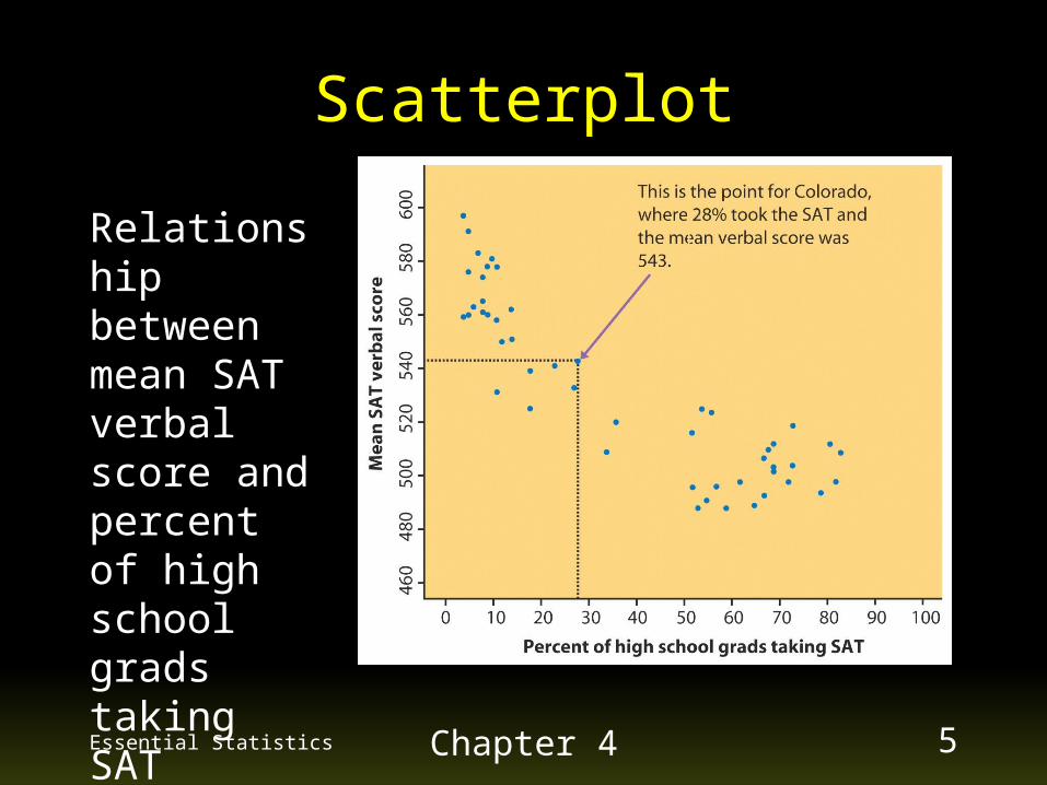
Graphs the relationship between two quantitative (numerical) variables measured on the same individuals.
Usually plot the explanatory variable on the horizontal (x) axis and plot the response variable on the vertical (y) axis.
Scatterplot
Essential Statistics Chapter 4 5
Relationship between mean SAT verbal score and percent of high school grads taking SAT
Scatterplot

Essential Statistics Chapter 4 6
Look for overall pattern and deviations from this pattern
Describe pattern by form, direction, and strength of the relationship
Look for outliers
Scatterplot

Essential Statistics Chapter 4 7
Linear Relationship
Some relationships are such that the points of a scatterplot tend to fall along a straight line -- linear relationship

Essential Statistics Chapter 4 8
Direction Positive association
◙ A positive value for the correlation implies a positive association.
◙ large values of X tend to be associated with large values of Y and small values of X
tend to be associated with small values of Y. Negative association
◙ A negative value for the correlation implies a negative or inverse association
◙ large values of X tend to be associated with small values of Y and vice versa.

Essential Statistics Chapter 4 9
Examples
From a scatterplot of college students, there is a positive association between verbal SAT score and GPA.
For used cars, there is a negative association between the age of the car and the selling price.

Essential Statistics Chapter 4 10
Examples of Relationships
0
10
20
30
40
50
60
$0 $10 $20 $30 $40 $50 $60 $70
Income
Hea
th S
tatu
s M
easu
re
0
10
20
30
40
50
60
70
0 20 40 60 80 100
Age
Hea
th S
tatu
s M
easu
re0
2
4
6
8
10
12
14
16
18
0 20 40 60 80 100
Age
Ed
uca
tion
Lev
el
30
35
40
45
50
55
60
65
0 20 40 60 80
Physical Health Score
Men
tal H
ealt
h S
core

Essential Statistics Chapter 4 11
Measuring Strength & Directionof a Linear Relationship
How closely does a straight line (non-horizontal) fit the points of a scatterplot?
The correlation coefficient (often referred to as just correlation): r– measure of the strength of the relationship:
the stronger the relationship, the larger the magnitude of r.
– measure of the direction of the relationship: positive r indicates a positive relationship, negative r indicates a negative relationship.

Essential Statistics Chapter 4 12
Correlation Coefficient special values for r :
a perfect positive linear relationship would have r = +1 a perfect negative linear relationship would have r = -1 if there is no linear relationship, or if the scatterplot
points are best fit by a horizontal line, then r = 0 Note: r must be between -1 and +1, inclusive
both variables must be quantitative; no distinction between response and explanatory variables
r has no units; does not change when measurement units are changed (ex: ft. or in.)

Essential Statistics Chapter 4 13
Examples of Correlations

Essential Statistics Chapter 4 14
Examples of Correlations
Husband’s versus Wife’s ages r = .94
Husband’s versus Wife’s heights r = .36
Professional Golfer’s Putting Success: Distance of putt in feet versus percent success
r = -.94
Essential Statistics Chapter 4 15
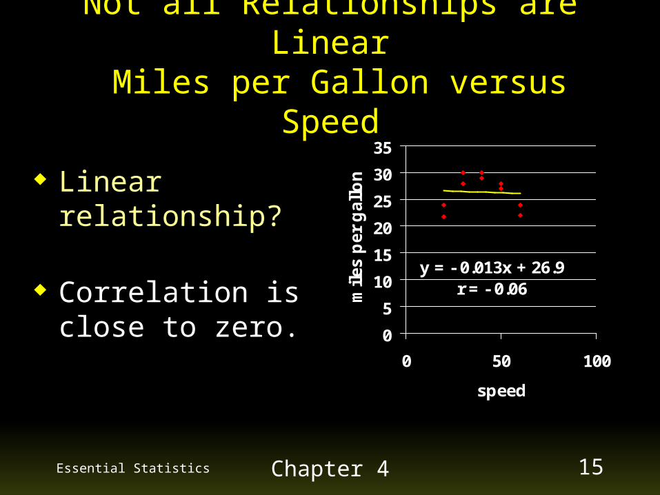
Not all Relationships are Linear Miles per Gallon versus Speed
Linear relationship?
Correlation is close to zero.
y = - 0.013x + 26.9r = - 0.06
0
5
10
15
20
25
30
35
0 50 100
speed
mil
es p
er
gall
on

Essential Statistics Chapter 4 16
Not all Relationships are Linear Miles per Gallon versus Speed
0
5
10
15
20
25
30
35
0 50 100
speed
mil
es p
er g
allo
n
Curved relationship.
Correlation is misleading.

Essential Statistics Chapter 4 17
Problems with Correlations
Outliers can inflate or deflate correlations (see next slide)
Groups combined inappropriately may mask relationships (a third variable)– groups may have different relationships
when separated

Essential Statistics Chapter 4 18
Outliers and Correlation
For each scatterplot above, how does the outlier affect the correlation?
A B
A: outlier decreases the correlation B: outlier increases the correlation

Essential Statistics Chapter 4 19
Correlation Calculation Suppose we have data on variables X
and Y for n individuals:x1, x2, … , xn and y1, y2, … , yn
Each variable has a mean and std dev:) for 2 ch. (see and s yx
s ,y (s ,x ( ))
n
1i y
i
x
i
s
yy
s
xx
1-n
1r
Essential Statistics Chapter 4 20
Case Study
Per Capita Gross Domestic Productand Average Life Expectancy for
Countries in Western Europe

Essential Statistics Chapter 4 21
Case Study
Country Per Capita GDP (x) Life Expectancy (y)
Austria 21.4 77.48
Belgium 23.2 77.53
Finland 20.0 77.32
France 22.7 78.63
Germany 20.8 77.17
Ireland 18.6 76.39
Italy 21.5 78.51
Netherlands 22.0 78.15
Switzerland 23.8 78.99
United Kingdom 21.2 77.37

Essential Statistics Chapter 4 22
Case Studyx y
21.4 77.48 -0.078 -0.345 0.027
23.2 77.53 1.097 -0.282 -0.309
20.0 77.32 -0.992 -0.546 0.542
22.7 78.63 0.770 1.102 0.849
20.8 77.17 -0.470 -0.735 0.345
18.6 76.39 -1.906 -1.716 3.271
21.5 78.51 -0.013 0.951 -0.012
22.0 78.15 0.313 0.498 0.156
23.8 78.99 1.489 1.555 2.315
21.2 77.37 -0.209 -0.483 0.101
= 21.52 = 77.754sum = 7.285
sx =1.532 sy =0.795
yi /syy xi /sxx
x y
y
i
x
i
s
y-y
s
x-x

Essential Statistics Chapter 4 23
Case Study
0.809
(7.285)110
1
n
1i y
i
x
i
s
yy
s
xx
1-n
1r

Summary Explanatory variable Vs responsible variable Scatterplot: display the relationship between two
quantitative variables measured on the same individuals Overall pattern of scatterplot showing:
☻ Direction ☻Form ☻ Strength♦ Correlation coefficient r: Measures only straight-line
linear relationship
♦ R indicate the direction of a linear relationship by sign
R > 0, positive association R< 0, negative association
♦ The range of R: -1 ≤ R ≤ 1,
Essential Statistics Chapter 4 24

ScatterplotsWhich of the following scatterplots displays the
stronger linear relationship?
a) Plot A
b) Plot B
c) Same for both

CorrelationIf two quantitative variables, X and Y, have a correlation coefficient r = 0.80, which graph could be a
scatterplot of the two variables?
a) Plot A
b) Plot B
c) Plot C
Plot A ? Plot B? Plot C?


