Test-case Generator for Nonlinear Continuous Parameter

Optimization Techniques

Zbigniew Michalewicz� , Kalyanmoy Deby , Martin Schmidtz, and Thomas Stidsenx

Abstract

The experimental results reported in many papers suggest that making an appropriate a priori choiceof an evolutionary method for a nonlinear parameter optimization problem remains an open question.It seems that the most promising approach at this stage of research is experimental, involving a designof a scalable test suite of constrained optimization problems, in which many features could be easilytuned. Then it would be possible to evaluate merits and drawbacks of the available methods as wellas test new methods e�ciently.

In this paper we propose such a test-case generator for constrained parameter optimization tech-niques. This generator is capable of creating various test problems with di�erent characteristics,like (1) problems with di�erent relative size of the feasible region in the search space; (2) problemswith di�erent number and types of constraints; (3) problems with convex or non-convex objectivefunction, possibly with multiple optima; (4) problems with highly non-convex constraints consistingof (possibly) disjoint regions. Such a test-case generator is very useful for analyzing and comparingdi�erent constraint-handling techniques.

Keywords: evolutionary computation, nonlinear programming, constrained optimization, test casegenerator

1 Introduction

The general nonlinear programming (NLP) problem is to �nd ~x so as to

optimize f(~x); ~x = (x1; : : : ; xn) 2 IRn; (1)

where ~x 2 F � S. The objective function f is de�ned on the search space S � IRn and the setF � S de�nes the feasible region. Usually, the search space S is de�ned as a n-dimensional rectanglein IRn (domains of variables de�ned by their lower and upper bounds):

li � xi � ui; 1 � i � n,

�Department of Computer Science, University of North Carolina, Charlotte, NC 28223, USA and at the Instituteof Computer Science, Polish Academy of Sciences, ul. Ordona 21, 01-237 Warsaw, Poland, e-mail: zbyszek@uncc.edu

yDepartment of Mechanical Engineering, Indian Institute of Technology, Kanpur, Pin 208 016, India, e-mail:deb@iitk.ac.in

zDepartment of Computer Science, Aarhus University, DK-8000 Aarhus C, Denmark, e-mail: marsch@daimi.au.dkxDepartment of Computer Science, Aarhus University, DK-8000 Aarhus C, Denmark, e-mail: stidsen@daimi.au.dk

whereas the feasible region F � S is de�ned by a set of p additional constraints (p � 0):

gj(~x) � 0, for j = 1; : : : ; q, and hj(~x) = 0, for j = q + 1; : : : ; p.

At any point ~x 2 F , the constraints gj that satisfy gj(~x) = 0 are called the active constraints at ~x.The NLP problem, in general, is intractable: it is impossible to develop a deterministic method

for the NLP in the global optimization category, which would be better than the exhaustive search(Gregory, 1995). This makes a room for evolutionary algorithms, extended by some constraint-handling methods. Indeed, during the last few years, several evolutionary algorithms (which aimat complex objective functions (e.g., non di�erentiable or discontinuous) have been proposed forthe NLP; a recent survey paper (Michalewicz and Schoenauer 1996) provides an overview of thesealgorithms.

It is not clear what characteristics of a constrained problem make it di�cult for an evolutionarytechnique (and, as a matter of fact, for any other optimization technique). Any problem can becharacterized by various parameters; these may include the number of linear constraints, the numberof nonlinear constraints, the number of equality constraints, the number of active constraints, theratio � = jFj=jSj of sizes of feasible search space to the whole, the type of the objective function (thenumber of variables, the number of local optima, the existence of derivatives, etc). In (Michalewiczand Schoenauer 1996) eleven test cases for constrained numerical optimization problems were pro-posed (G1{G11). These test cases include objective functions of various types (linear, quadratic,cubic, polynomial, nonlinear) with various number of variables and di�erent types (linear inequal-ities, nonlinear equations and inequalities) and numbers of constraints. The ratio � between thesize of the feasible search space F and the size of the whole search space S for these test cases varyfrom 0% to almost 100%; the topologies of feasible search spaces are also quite di�erent. These testcases are summarized in Table 1. For each test case the number n of variables, type of the functionf , the relative size of the feasible region in the search space given by the ratio �, the number ofconstraints of each category (linear inequalities LI, nonlinear equations NE and inequalities NI),and the number a of active constraints at the optimum (including equality constraints) are listed.

The results of many tests did not provide meaningful conclusions, as no single parameter (numberof linear, nonlinear, active constraints, the ratio �, type of the function, number of variables)proved to be signi�cant as a major measure of di�culty of the problem. For example, many testedmethods approached the optimum quite closely for the test cases G1 and G7 (with � = 0:0111%and � = 0:0003%, respectively), whereas most of the methods experienced di�culties for the testcase G10 (with � = 0:0010%). Two quadratic functions (the test cases G1 and G7) with a similarnumber of constraints (9 and 8, respectively) and an identical number (6) of active constraints atthe optimum, gave a di�erent challenge to most of these methods. Also, several methods were quitesensitive to the presence of a feasible solution in the initial population. Possibly a more extensivetesting of various methods was required.

Not surprisingly, the experimental results of (Michalewicz and Schoenauer 1996) suggested thatmaking an appropriate a priori choice of an evolutionary method for a nonlinear optimizationproblem remained an open question. It seems that more complex properties of the problem (e.g.,the characteristic of the objective function together with the topology of the feasible region) mayconstitute quite signi�cant measures of the di�culty of the problem. Also, some additional measuresof the problem characteristics due to the constraints might be helpful. However, this kind ofinformation is not generally available. In (Michalewicz and Schoenauer 1996) the authors wrote:

\It seems that the most promising approach at this stage of research is experimental,involving the design of a scalable test suite of constrained optimization problems, in

2

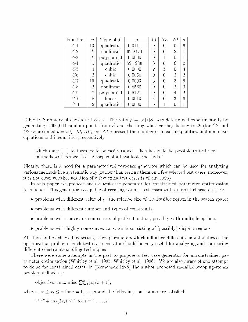
Function n Type of f � LI NE NI a

G1 13 quadratic 0.0111% 9 0 0 6G2 k nonlinear 99.8474% 0 0 2 1G3 k polynomial 0.0000% 0 1 0 1G4 5 quadratic 52.1230% 0 0 6 2G5 4 cubic 0.0000% 2 3 0 3G6 2 cubic 0.0066% 0 0 2 2G7 10 quadratic 0.0003% 3 0 5 6G8 2 nonlinear 0.8560% 0 0 2 0G9 7 polynomial 0.5121% 0 0 4 2G10 8 linear 0.0010% 3 0 3 6G11 2 quadratic 0.0000% 0 1 0 1

Table 1: Summary of eleven test cases. The ratio � = jFj=jSj was determined experimentally bygenerating 1,000,000 random points from S and checking whether they belong to F (for G2 andG3 we assumed k = 50). LI, NE, and NI represent the number of linear inequalities, and nonlinearequations and inequalities, respectively

which many [...] features could be easily tuned. Then it should be possible to test newmethods with respect to the corpus of all available methods."

Clearly, there is a need for a parameterized test-case generator which can be used for analyzingvarious methods in a systematic way (rather than testing them on a few selected test cases; moreover,it is not clear whether addition of a few extra test cases is of any help).

In this paper we propose such a test-case generator for constrained parameter optimizationtechniques. This generator is capable of creating various test cases with di�erent characteristics:

� problems with di�erent value of �: the relative size of the feasible region in the search space;

� problems with di�erent number and types of constraints;

� problems with convex or non-convex objective function, possibly with multiple optima;

� problems with highly non-convex constraints consisting of (possibly) disjoint regions.

All this can be achieved by setting a few parameters which in uence di�erent characteristics of theoptimization problem. Such test-case generator should be very useful for analyzing and comparingdi�erent constraint-handling techniques.

There were some attempts in the past to propose a test case generator for unconstrained pa-rameter optimization (Whitley et al. 1995; Whitley et al. 1996). We are also aware of one attemptto do so for constrained cases; in (Kemenade 1998) the author proposed so-called stepping-stonesproblem de�ned as:

objective: maximizePn

i=1(xi=� + 1),

where �� � xi � � for i = 1; : : : ; n and the following constraints are satis�ed:

exi=� + cos(2xi) � 1 for i = 1; : : : ; n.

3

Note that the objective function is linear and that the feasible region is split into 2n disjoint parts(called stepping-stones). As the number of dimensions n grows, the problem becomes more complex.However, as the stepping-stones problem has one parameter only, it can not be used to investigatesome aspects of a constraint-handling method. In (Michalewicz et al., 1999a; Michalewicz et al.,1999b) we reported on preliminary experiments with a test case generator.

The paper is organized as follows. The following section describes the proposed test-case genera-tor for constrained parameter optimization techniques. Section 3 surveys brie y several constraint-handling techniques for numerical optimization problems which have emerged in evolutionary com-putation techniques over the last years. Section 4 discusses experimental results of one particularconstraint-handling technique on a few generated test cases. Section 5 concludes the paper andindicates some directions for future research.

2 Test-case generator

As explained in the Introduction, it is of great importance to have a parameterized generator of testcases for constrained parameter optimization problems. By changing values of some parameters itwould be possible to investigate merits/drawbacks (e�ciency, cost, etc) of many constraint-handlingmethods. Many interesting questions could be addressed:

� how the e�ciency of a constraint-handling method changes as a function of the number ofdisjoint components of the feasible part of the search space?

� how the e�ciency of a constraint-handling method changes as a function of the ratio betweenthe sizes of the feasible part and the whole search space?

� what is the relationship between the number of constraints (or the number of dimensions, forexample) of a problem and the computational e�ort of a method?

and many others. In the following part of this section we describe such parameterized test-casegenerator

T CG(n;w; �; �; �; �);

the meaning of its six parameters is as follows:

n { the number of variables of the problemw { a parameter to control the number of optima in the search space� { a parameter to control the number of constraints (inequalities)� { a parameter to control the connectedness of the feasible search regions� { a parameter to control the ratio of the feasible to total search space� { a parameter to in uence the ruggedness of the �tness landscape

The following subsection explains the general ideas behind the proposed concepts. Subsection2.2 describes some details of the test-case generator T CG, and subsection 2.3 graphs a few land-scapes. Subsection 2.4 discusses further enhancements incorporated in the T CG, and subsection 2.5summarizes some of its properties.

4

2.1 Preliminaries

The general idea is to divide the search space S into a number of disjoint subspaces Sk and to de�nea unimodal function fk for every Sk. Thus the objective function G is de�ned on S as follows:

G(~x) = fk(~x) i� ~x 2 Sk.The number of subspaces Sk corresponds to the total number of local optima of function G.

Each subspace Sk is divided further into its feasible Fk and infeasible Ik parts; it may happen,that one of these parts is empty. This division of Sk is obtained by introduction of a doubleinequality which feasible points must satisfy. The feasible part F of the whole search space S isde�ned then as a union of all Fk's.

The �nal issue addressed in the proposed model concerns the relative heights of local optima offunctions fk. The global optimum is always located in S0, but the heights of other peaks (i.e., localoptima) may determine whether the problem would be easier or harder to solve.

Let us discuss now the connections between the above ideas and the parameters of the test-casegenerator. The �rst (integer) parameter n of the T CG determines the number of variables of theproblem; clearly, n � 1. The next (integer) parameter w � 1 determines the number of local optimain the search space, as the search space S is divided into wn disjoint subspaces Sk (0 � k � wn� 1)and there is a unique unconstrained optimum in each Sk. The subspaces Sk are de�ned in section2.2; however, the idea is to divide the domain of each of n variables into w disjoint and equalsized segments of the length 1

w. The parameter w determines also the boundaries of the domains

of all variables: for all 1 � i � n, xi 2 [� 12w ; 1 � 1

2w ). Thus the search space S is de�ned as an-dimensional rectangle:1

S =Qn

i=1[� 12w ; 1� 1

2w );

consequently jSj = 1.The third parameter � of the test-case generator is related to the number m of constraints of the

problem, as the feasible part F of the search space S is de�ned by means on m double inequalities,called \rings" or \hyper-spheres", (1 � m � wn):

r21 � ck(~x) � r22; k = 0; : : : ;m� 1; (2)

where 0 � r1 � r2 and each ck(~x) is a quadratic function:

ck(~x) = (x1 � pk1)2 + : : : + (xn � pkn)2,

where (pk1; : : : ; pkn) is the center of the kth ring.

These m double inequalities de�ne m feasible parts Fk of the search space:

~x 2 Fk i� r21 � ck(~x) � r22,

and the overall feasible search space F = [m�1k=0 Fk. Note, the interpretation of constraints here isdi�erent than the one in the standard de�nition of the NLP problem (see Equation (1)): Here thesearch space F is de�ned as a union (not intersection) of all double constraints. In other words, a

1In section 2.4 we de�ne an additional transformation from [� 1

2w; 1� 1

2w) to [0; 1) to simplify the usability of the

T CG.

5

point ~x is feasible if and only if there exist an index 0 � k � m� 1 such that double inequality inEquation (2) is satis�ed. Note also, that if m < wn, then Fk are empty for all m � k � wn � 1.

The parameter 0 � � � 1 determines the number m of constraints as follows:

m = b�(wn � 1) + 1c: (3)

Clearly, � = 0 and � = 1 imply m = 1 and m = wn, i.e., minimum and maximum number ofconstraints, respectively.

There is one important implementational issue connected with a representation of the numberwn. This number might be too large to store as an integer variable in a program (e.g., for w = 10 andn = 500); consequently the value of m might be too large as well. Because of that the Equation (3)should be interpreted as the expected value of random variable m rather than the exact formula.This is achieved as follows. Note that an index k of a subspace Sk can be represented in a n-dimensional w-ary alphabet (for w > 1) as (q1;k; : : : ; qn;k), i.e.,

k =Pn

i=1 qi;kwn�i.

Then, for each dimension, we (randomly) select a fraction (�)1

n of indices; the subspace Sk containsone of m constraints i� an index qi;k was selected for dimension i (1 � i � n). Note that theprobability of selecting any subspace Sk is �. For the same reason later in the paper (see sections2.2 and 2.5), new parameters (k0 and k00) replace the original k (e.g., Equations (21) and (28)). Thecenter (pk1; : : : ; p

kn) of a hyper-sphere de�ned by a particular ck (0 � k � m � 1) is determined as

follows:(pk1; : : : ; p

kn) = (qn;k=w; : : : ; q1;k=w); (4)

where (q1;k; : : : ; qn;k) is a n-dimensional representation of the number k in w-ary alphabet.2

Let us illustrate concepts introduced so far by the following example. Assume n = 2, w = 5,and m = 22 (note that m � wn). Let us assume that r1 and r2 (smaller and larger radii of allhyper-spheres (circles in this case), respectively) have the following values:3

r1 = 0:04 and r2 = 0:09.

Thus the feasible search space consists of m = 22 disjoint rings, and the ratio � between thesizes of the feasible part F and the whole search space S is 0.449. The search space S and thefeasible part F are displayed in Figure 1(a).

Note that the center of the \�rst" sphere de�ned by c0 (i.e., k = 0) is (p01; p02) = (0; 0), as

k = 0 = (0; 0)5. Similarly, the center of the \fourteenth" sphere (out of m = 22) de�ned by c13 (i.e.,k = 13) is (p131 ; p

132 ) = (3=w; 2=w), as k = 13 = (2; 3)5.

With r2 = 0 (which also implies r1 = 0), the feasible search space would consist of a set of mpoints. It is interesting to note that for r1 = 0:

� if 0 � r2 <12w , the feasible search space F consists of m disjoint convex components; however

the overall search space is non-convex;

2We assumed here, that w > 1; for w = 1 there is no distinction between the search space S and the subspace S0,and consequently m is one (a single double constraint). In the latter case, the center of the only hyper-sphere is thecenter of the search space.

3These values are determined by two other parameters of the test-case generator, � and �, as discussed later.

6

x

x2

1

1/w 2/w 3/w 4/w

w = 5

1/w

2/w

3/w

4/w

(1-1/(2w), 1-1/(2w))

(1-1/(2w), -1/(2w))(-1/(2w), -1/(2w))

(-1/(2w), 1-1/(2w))

(a)

x

x2

1

1/w 2/w 3/w 4/w

w = 5

1/w

2/w

3/w

4/w

(1-1/(2w), 1-1/(2w))(-1/(2w), 1-1/(2w))

(-1/(2w), -1/(2w)) (1-1/(2w), -1/(2w))

(b)

Figure 1: The search spaces S and their feasible parts F (shaded areas) for test cases with n = 2,m = 22, r1 = 0:04, and (a) r2 = 0:09 or (b) r2 = 0:12

� if 12w � r2 <

pn

2w , the feasible search space F consists of one connected component; however,this component is highly non-convex with many \holes" among spheres (see Figure 2(a));

� if r2 =pn

2w , most of the whole search space would be feasible (except the \right-top corner" ofthe search space due to the fact that the number of spheres m might be smaller than wn; seeFigure 2(b)). In any case, F consists of a single connected component.4

Based on the above discussions, we can assume that radii r1 and r2 satisfy the following inequal-ities:

0 � r1 � r2 �pn

2w: (5)

Now we can de�ne the fourth and �fth control parameters of the test-case generator T CG:

� =2wr2p

n; (6)

� =r1r2: (7)

The operating range for � and � is 0 � �; � � 1. In that way, the radii r1 and r2 are de�ned bythe parameters of the test-case generator:

r1 =��pn

2w; r2 =

�pn

2w: (8)

Note that if � < 1=pn, the feasible `islands' Fk are not connected, as discussed above. On the

other hand, for � � 1=pn, the feasible subspaces Fk are connected. Thus, the parameter � controls

the connectedness of the feasible search space.5

4Note that the exact value of � depends on m: if m = wn, then � = 1; otherwise, � < 1.5We shall see later, that this parameter, together with parameter �, also controls the amount of deviation of the

constrained maximum solution from the unconstrained maximum solution.

7

x

x2

1

1/w 2/w 3/w 4/w

w = 5

1/w

2/w

3/w

4/w

(-1/(2w), 1-1/(2w)) (1-1/(2w), 1-1/(2w))

(-1/(2w), -1/(2w)) (1-1/(2w), -1/(2w))

(a)

x

x2

1

1/w 2/w 3/w 4/w

w = 5

1/w

2/w

3/w

4/w

(-1/(2w), 1-1/(2w)) (1-1/(2w), 1-1/(2w))

(-1/(2w), -1/(2w)) (1-1/(2w), -1/(2w))

(b)

Figure 2: The search spaces S and their feasible parts F (shaded areas) for test cases with n = 2,

m = 22, r1 = 0, and (a) r2 = 0:12 or (b) r2 =p2

2w=

p2

10

For � = 0 the feasible parts Fk are convex and for � > 0 | always non-convex (see (a) and(b) of Figure 1). If � = 1 (i.e, r1 = r2), the feasible search space consists of (possibly parts of)boundaries of spheres; this case corresponds to an optimization problem with equality constraints.The parameter � is also related to the proportion of the ratio � of the feasible to the total searchspace (� = jFj=jSj). For an n-dimensional hyper-sphere, the enclosed volume is given as follows(Rudolph, 1996):

Vn(r) =�n=2rn

�(n=2 + 1): (9)

When � � 1=pn, the ratio � can be written as follows6 (note that jSj = 1):

� = m (Vn(r2)� Vn(r1)) =(�n)n=2�n

2n�(n=2 + 1)

m

wn(1� �n) : (10)

When � � 1 (Fk's are rings of a small width), the above ratio is

� � (�n)n=2�n

2n�(n=2 + 1)

m

wnn(1� �): (11)

In the following subsection, we de�ne the test-case generator T CG in detail; we provide de�nitionsof functions fk and discuss the sixth parameter � of this test-case generator.

6For � > 1, the hyper-spheres overlap and it is not trivial to compute this ratio. However, this ratio gets closerto one as � increases from one.

8

2.2 Details

As mentioned earlier, the search space S =Qn

i=1[� 12w; 1� 1

2w) is divided into wn subspaces Sk, k =

0; 1; : : : ; (wn � 1). Each subspace Sk is de�ned as a n-dimensional cube: Sk = fxi : lki � xi < uki g,where the bounds lki and uki are de�ned as:

lki =2qn�i+1;k � 1

2wand uki =

2qn�i+1;k + 1

2w; (12)

for k = 0; 1; : : : ; (wn�1). The parameter qn�i+1;k is the (n� i+1)-th component of a n-dimensionalrepresentation of the number k in w-ary alphabet. For example, the boundaries of the subspace S13(see Figure 1) are

52w� x1 <

72w

and 32w� x2 <

52w

,

as (2; 3)5 = 13, i.e., (2; 3) is a 2-dimensional representation of k = 13 in w = 5-ary alphabet.For each subspace Sk, there is a function fk de�ned on this subspace as follows:

fk(x1; : : : ; xn) = ak��n

i=1(uki � xi)(xi � lki )

� 1

n ; (13)

where ak's are prede�ned positive constants. Note that for any ~x 2 Sk, fk(~x) � 0; moreover,fk(~x) = 0 i� ~x is a boundary point of the subspace Sk.

The objective function (to be maximized) of the test-case generator T CG is de�ned as follows:

G(x1; : : : ; xn) =

8>>>>>>>><>>>>>>>>:

f0(x1; : : : ; xn) if (x1; : : : ; xn) 2 S0f1(x1; : : : ; xn) if (x1; : : : ; xn) 2 S1:::fwn�1(x1; : : : ; xn) if (x1; : : : ; xn) 2 Swn�1,

(14)

where

� � 12w � xi < 1 � 1

2w for all 1 � i � n, i.e., ~x = (x1; : : : ; xn) 2 S, and

� F = F0 [ ::: [ Fwn�1, i.e., one of the following m double constraints is satis�ed:

r21 � ck � r22 (0 � k � m� 1).

Now we are ready to discuss the signi�cance of the prede�ned constants ak (Equation (13)). Letus introduce the following notation:

� (xk1; : : : ; xkn) { is the maximum solution for unconstrained function fk, i.e., when the constraint

r21 � ck(~x) � r22 is ignored (with r1 > 0),

� (�xk1; : : : ; �xkn) { is the maximum solution for constrained function fk, i.e., when the constraintr21 � ck(~x) � r22 is taken into account.

It is obvious, that the function fk has its unconstrained maximum at the center of Sk, i.e.,

9

xki = (lki + uki )=2.

The corresponding function value at this point is

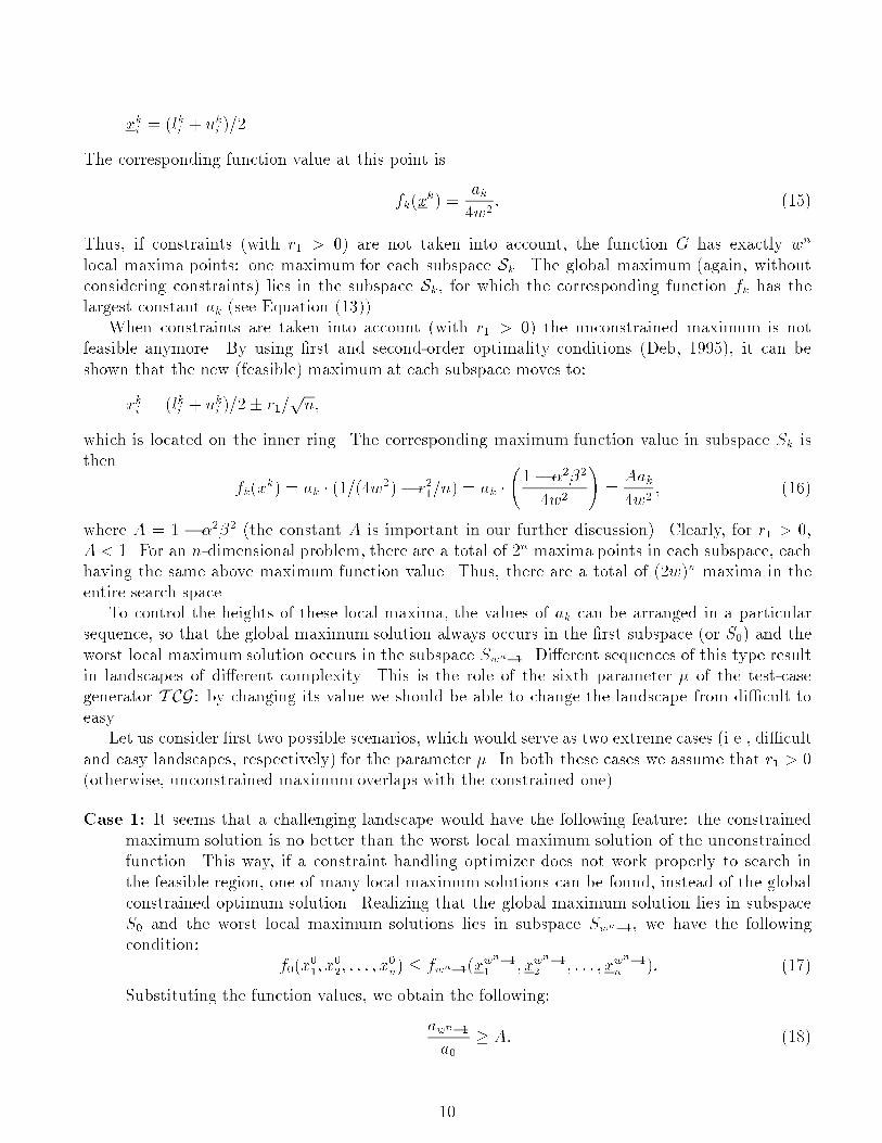
fk(xk) =

ak4w2

: (15)

Thus, if constraints (with r1 > 0) are not taken into account, the function G has exactly wn

local maxima points: one maximum for each subspace Sk. The global maximum (again, withoutconsidering constraints) lies in the subspace Sk, for which the corresponding function fk has thelargest constant ak (see Equation (13)).

When constraints are taken into account (with r1 > 0) the unconstrained maximum is notfeasible anymore. By using �rst and second-order optimality conditions (Deb, 1995), it can beshown that the new (feasible) maximum at each subspace moves to:

�xki = (lki + uki )=2� r1=pn,

which is located on the inner ring. The corresponding maximum function value in subspace Sk isthen

fk(�xk) = ak � (1=(4w2)� r21=n) = ak �

1� �2�2

4w2

!=

Aak4w2

; (16)

where A = 1 � �2�2 (the constant A is important in our further discussion). Clearly, for r1 > 0,A < 1. For an n-dimensional problem, there are a total of 2n maxima points in each subspace, eachhaving the same above maximum function value. Thus, there are a total of (2w)n maxima in theentire search space.

To control the heights of these local maxima, the values of ak can be arranged in a particularsequence, so that the global maximum solution always occurs in the �rst subspace (or S0) and theworst local maximum solution occurs in the subspace Swn�1. Di�erent sequences of this type resultin landscapes of di�erent complexity. This is the role of the sixth parameter � of the test-casegenerator T CG: by changing its value we should be able to change the landscape from di�cult toeasy.

Let us consider �rst two possible scenarios, which would serve as two extreme cases (i.e., di�cultand easy landscapes, respectively) for the parameter �. In both these cases we assume that r1 > 0(otherwise, unconstrained maximum overlaps with the constrained one).

Case 1: It seems that a challenging landscape would have the following feature: the constrainedmaximum solution is no better than the worst local maximum solution of the unconstrainedfunction. This way, if a constraint handling optimizer does not work properly to search inthe feasible region, one of many local maximum solutions can be found, instead of the globalconstrained optimum solution. Realizing that the global maximum solution lies in subspaceS0 and the worst local maximum solutions lies in subspace Swn�1, we have the followingcondition:

f0(�x01; �x02; : : : ; �x0n) � fwn�1(xwn�11 ; xw

n�12 ; : : : ; xw

n�1n ): (17)

Substituting the function values, we obtain the following:

awn�1a0

� A: (18)

10

Case 2: On the other hand, let us consider an easy landscape, where the constrained maximumsolution is no worse than the unconstrained local maximum solution of the next-best subspace.This makes the function easy to optimize, because the purpose is served even if the constraintoptimizer is incapable of distinguishing feasible and infeasible regions in the search space, aslong as it can �nd the globally best subspace in the entire search space and concentrate itssearch there. Note that even in this case there are many local maximum solutions where theoptimizer can get stuck to. Thus, this condition tests more an optimizer's ability to �nd theglobal maximum solution among many local maximum solutions and does not test too muchwhether the optimizer can distinguish feasible from infeasible search regions. Mathematically,the following condition must be true:

f0(�x01; �x02; : : : ; �x0n) � f1(x11; x

12; : : : ; x

1n); (19)

assuming that the next-base subspace is S1. Substituting the function values, we obtain

a1a0� A: (20)

Thus, to control the degree of di�culty in the function, i.e., to vary between cases 1 and 2, theparameter � is introduced. It can be adjusted at di�erent values to have the above two conditionsas extreme cases. To simplify the matter, we may like to have Condition (18) when � is set to oneand have Condition (20) when � is set to zero. One such possibility is to have the following termfor de�ning ak:7

ak = (1� �2�2)(1��0)k0

= A(1��0)k0

: (21)

The value of k0 is given by the following formula

k0 = log2(nXi=1

qi;k + 1); (22)

where (q1;k; : : : ; qn;k) is a n-dimensional representation of the number k in w-ary alphabet. Thevalue of �0 is de�ned as

�0 =

1� 1

log2(nw � n + 1)

!�; (23)

for � 2 [0; 1]. The term from Equation (21) has the following properties:

1. All ak are non-negative.

2. The value of a0 for the �rst subspace S0 is always one as a0 = A0 = 1.

3. The sequence ak takes n(w � 1) + 1 di�erent values (for k = 0; : : : ; wn � 1).

4. For � = 0, the sequence ak = Ak0

lies in [Alog2(nw�n+1); 1] (with a0 = 1 and awn�1 =

Alog2(nw�n+1)). Note that a1 = A1 = A, so Condition (20) is satis�ed. Thus, setting �0 = 0

makes the test function much easier, as discussed above.

7Although this term can be used for any w � 1, we realize that for w = 1 there is only one subspace S0 and a0 is1, irrespective of �. For completeness, we set � = 1 in this case.

11

5. For � = 1, the sequence ak = Ak0= log2(nw�n+1) lies in the range [A; 1] (with a0 = 1 and

awn�1 = A) and Condition (18) is satis�ed with the equality sign. Thus we have Case 1established which is the most di�cult test function of this generator, as discussed above.

Since � = 0 and � = 1 are two extreme cases of easiness and di�culty, test functions with variouslevels of di�culties can be generated by using � 2 [0; 1]. Values of � closer to one will create moredi�cult test functions than values closer to zero. In the next section, we show the e�ect of varying� in some two-dimensional test functions.

To make the global constrained maximum function value always at 1, we normalize the akconstants as follows:

a0k =ak

(1=(4w2)� r21=n)=

4w2

1� �2�2

!� ak = 4w2(1� �2�2)k

0(1��0)�1; (24)

where k0 and �0 are de�ned by Equations (22) and (23), respectively. Thus, the proposed testfunction generator is de�ned in Equation (14), where the functions fk are de�ned in Equation (13).The term ak in Equation (13) is replaced by a0k de�ned in Equation (24). The global maximumsolution is at xi = �r1=

pn = ���=(2w) for all i = 1; 2; : : : ; n and the function values at these

solutions are always equal to one. It is important to note that there are a total 2n global maximumsolutions having the same function value of one and at all these maxima, only one constraint(c0(~x) � r21) is active.

Let us emphasize again that the above discussion is relevant only for r1 > 0. If r1 = 0, thenA = 1��2�2 = 1, and all ak's are equal to one. Thus we need a term de�ning ak if �� = 0 to makepeaks of variable heights. In this case we can set

ak =(�� 1)k00

n(w � 1)+ 1; (25)

The value of k00 is given by the following formula

k00 =Pn

i=1 qi;k,

where (q1;k; : : : ; qn;k) is a n-dimensional representation of the number k in w-ary alphabet. Thus,for � = 0 we have a0 = 1 and awn�1 = 0 (the steepest decline of heights of the peaks), whereas for� = 1, a0 = a1 = : : : = awn�1 = 1 (no decline). To make sure the global maximum value of theconstrained function is equal to 1, we can set

a0k = 4w2ak (26)

for all k.

2.3 A few examples

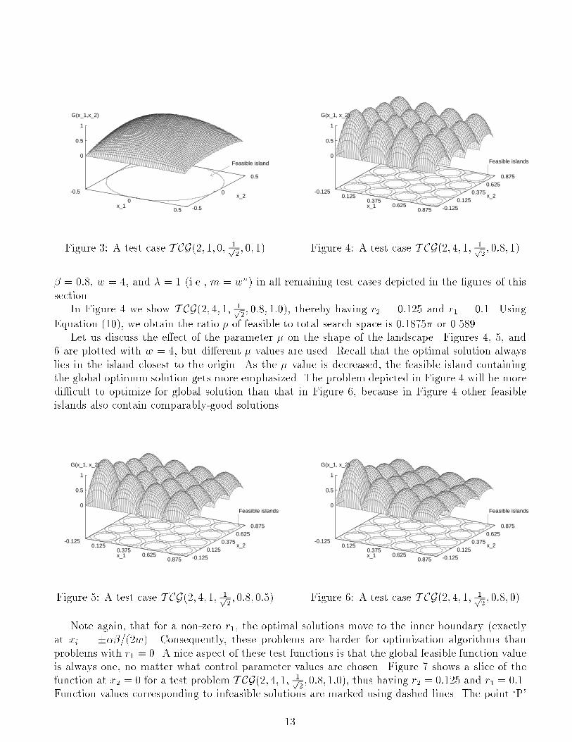
In order to get a feel for the objective function at this stage of building the T CG, we plot the surfacefor di�erent values of control parameters and with n = 2 (two variables only). A very simple uni-modal test problem can be generated by using the following parameter setting: T CG(2; 1; 0; 1p

2; 0; 1)

(see Figure 3). Note that in this case � = 0 which implies r1 = 0 (see (21)). To show the reducingpeak e�ect we need w > 1 and � > 0, as for � = 0 all peaks have the same height. Thus we assume

12

Feasible island

-0.5

0

0.5 -0.5

0

0.5

0

0.5

1

x_1

x_2

G(x_1,x_2)

Figure 3: A test case T CG(2; 1; 0; 1p2; 0; 1)

Feasible islands

-0.1250.125

0.3750.625

0.875 -0.1250.125

0.3750.625

0.875

0

0.5

1

x_1

x_2

G(x_1, x_2)

Figure 4: A test case T CG(2; 4; 1; 1p2; 0:8; 1)

� = 0:8, w = 4, and � = 1 (i.e., m = wn) in all remaining test cases depicted in the �gures of thissection.

In Figure 4 we show T CG(2; 4; 1; 1p2; 0:8; 1:0), thereby having r2 = 0:125 and r1 = 0:1. Using

Equation (10), we obtain the ratio � of feasible to total search space is 0:1875� or 0.589.Let us discuss the e�ect of the parameter � on the shape of the landscape. Figures 4, 5, and

6 are plotted with w = 4, but di�erent � values are used. Recall that the optimal solution alwayslies in the island closest to the origin. As the � value is decreased, the feasible island containingthe global optimum solution gets more emphasized. The problem depicted in Figure 4 will be moredi�cult to optimize for global solution than that in Figure 6, because in Figure 4 other feasibleislands also contain comparably-good solutions.

Feasible islands

-0.1250.125

0.3750.625

0.875 -0.1250.125

0.3750.625

0.875

0

0.5

1

x_1

x_2

G(x_1, x_2)

Figure 5: A test case T CG(2; 4; 1; 1p2; 0:8; 0:5)

Feasible islands

-0.1250.125

0.3750.625

0.875 -0.1250.125

0.3750.625

0.875

0

0.5

1

x_1

x_2

G(x_1, x_2)

Figure 6: A test case T CG(2; 4; 1; 1p2; 0:8; 0)

Note again, that for a non-zero r1, the optimal solutions move to the inner boundary (exactlyat xi = ���=(2w). Consequently, these problems are harder for optimization algorithms thanproblems with r1 = 0. A nice aspect of these test functions is that the global feasible function valueis always one, no matter what control parameter values are chosen. Figure 7 shows a slice of thefunction at x2 = 0 for a test problem T CG(2; 4; 1; 1p

2; 0:8; 1:0), thus having r2 = 0:125 and r1 = 0:1.

Function values corresponding to infeasible solutions are marked using dashed lines. The point `P'

13

is the globally optimal function value. The infeasible function values (like point `Q') higher than oneare also shown. If the constraint handling strategy is not proper, an optimization algorithm mayget trapped in local optimal solutions, like `Q', which has better function value but is infeasible.

0

0.2

0.4

0.6

0.8

1

1.2

1.4

1.6

-0.125 0 0.125 0.25 0.375 0.5 0.625 0.75 0.875

Fun

ctio

n va

lue

x_1

Infeasible function values

P

Q

Figure 7: A slice through x2 = 0 of a test problem with w = 4, � = 1:0, and r1 = 0:1 is shown. Theglobal optimum solution is in the left-most attractor

2.4 Further enhancements

As explained in section 2.1, the general idea behind the test-case generator T CG was to divide thesearch space S into a number of disjoint subspaces Sk and to de�ne an unimodal function fk forevery Sk. The number of subspaces Sk corresponds to the total number of local optima of functionG. To control the heights of these local maxima, the values of ak were arranged in a particularsequence, so that the global maximum solution always occurs in the �rst subspace (for k = 0, i.e., inS0) and the worst local maximum solution occurs in the last subspace (for k = wn�1, i.e., in Swn�1).Note also that subspaces Sk of the test-case generator T CG are arranged in a particular order. Forexample, for n = 2 and w = 4, the highest peak is located in subspace S0, two next-highest peaks(of the same height) are in subspaces S1 and S4, three next-highest peaks are in S2, S5, S8, etc.(see Figures 4{6).

To remove this �xed pattern from the generated test cases, we need an additional mechanism:a random permutation of subspaces Sk. Thus we need a procedure Transform which randomlypermutes indices of subspaces; this is any function

Transform: [0::N ] �! [0::N ],

such that for any 0 � p 6= q � N , Transform(p) 6= Transform(q). The advantage of such a procedureTransform is that we do not need any memory for storing the mapping between indices of subspaces(the size of such memory, for w > 1 and large n, may be excessive); however, there is a need tore-compute the permuted index of a subspace Sk every time we need it.

The procedure Transform can be used also to generate a di�erent allocation for m constraints.Note that the T CG allocates m rings (each de�ned by a pair of constraints) always to the �rst m

14

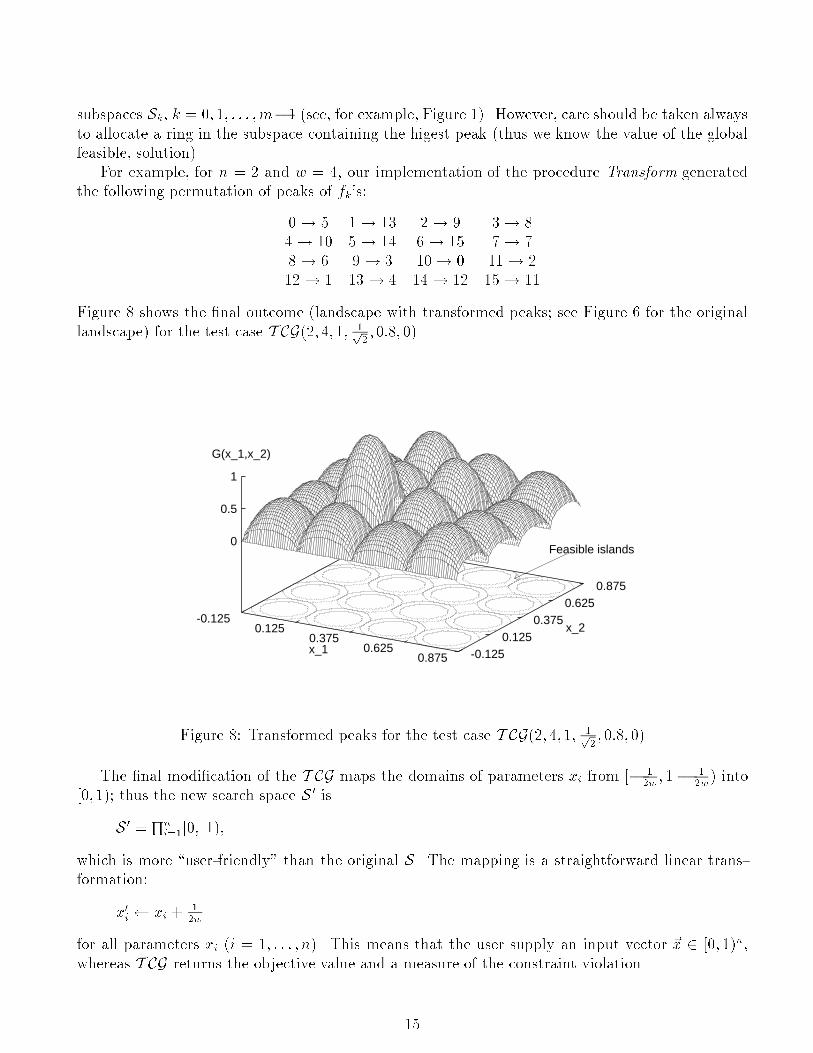
subspaces Sk, k = 0; 1; : : : ;m�1 (see, for example, Figure 1). However, care should be taken alwaysto allocate a ring in the subspace containing the higest peak (thus we know the value of the globalfeasible, solution).

For example, for n = 2 and w = 4, our implementation of the procedure Transform generatedthe following permutation of peaks of fk's:

0! 5 1! 13 2! 9 3! 84! 10 5! 14 6! 15 7! 78! 6 9! 3 10! 0 11! 212! 1 13! 4 14! 12 15! 11

Figure 8 shows the �nal outcome (landscape with transformed peaks; see Figure 6 for the originallandscape) for the test case T CG(2; 4; 1; 1p

2; 0:8; 0).

Feasible islands

-0.1250.125

0.3750.625

0.875 -0.1250.125

0.3750.625

0.875

0

0.5

1

x_1

x_2

G(x_1,x_2)

Figure 8: Transformed peaks for the test case T CG(2; 4; 1; 1p2; 0:8; 0)

The �nal modi�cation of the T CG maps the domains of parameters xi from [� 12w ; 1� 1

2w ) into[0; 1); thus the new search space S 0 is

S 0 =Qn

i=1[0; 1),

which is more \user-friendly" than the original S. The mapping is a straightforward linear trans-formation:

x0i xi + 12w

for all parameters xi (i = 1; : : : ; n). This means that the user supply an input vector ~x 2 [0; 1)n,whereas T CG returns the objective value and a measure of the constraint violation.

15

2.5 Summary

Based on the above presentations, we now summarize the properties of the test-case generator

T CG(n;w; �; �; �; �).

The parameters are:

n � 1; integer w � 1; integer 0 � � � 1; oat0 � � � 1; oat 0 � � � 1; oat 0 � � � 1; oat

The objective function G is de�ned by formula (14), where each fk (k = 0; : : : ; wn � 1) is de�nedon Sk as

fk(x01; : : : ; x

0n) = a0k

��n

i=1(uki � xi)(xi � lki )

� 1

n : (27)

All variables x0i's have the same domain:

x0i 2 [0; 1).

Note, that x0i = xi + 12w

. The constants a0k are de�ned as follows:

a0k =

(4w2(1� �2�2)k

0[(1��)+�=(log2(wn�n+1)]�1 if �� > 0

4w2�(��1)k00

n(w�1) + 1�

if �� = 0,(28)

where

k0 = log2(Pn

i=1 qi;k + 1), andk00 =

Pni=1 qi;k,

where (q1;k; : : : ; qn;k) is a n-dimensional representation of the number k in w-ary alphabet.If r1 > 0 (i.e., �� > 0), the function G has 2n global maxima points, all in permuted S0. For

any global solution (x1; : : : ; xn), xi = ���=(2w) for all i = 1; 2; : : : ; n. The function values at thesesolutions are always equal to one.

On the other hand, if r1 = 0 (i.e., �� = 0), the function G has either one global maximum (if� < 1) or m maxima points (if � = 1), one in each of permuted S0; : : : ;Sm�1. If � < 1, the globalsolution (x1; : : : ; xn) is always at

(x1; : : : ; xn) = (0; 0; : : : ; 0).

The interpretation of the six parameters of the test-case generator T CG is as follows:

1. Dimensionality n: By increasing the parameter n the dimensionality of the search space canbe increased.

2. Multimodality w: By increasing the parameter w the multimodality of the search space canbe increased. For the unconstrained function, there are wn local maximum solutions, of whichone is globally maximum. For the constrained test function with �� > 0, there are (2w)n

di�erent local maximum solutions, of which 2n are globally maximum solutions.

3. Number of constraints �: By increasing the parameter � the number m of constraints isincreased.

16

4. Connectedness �: By reducing the parameter � (from 1 to 1=pn and smaller), the con-

nectedness of the feasible subspaces can be reduced. When � < 1=pn, the feasible subspaces

Fk are completely disconnected. Additionally, parameter � (with �xed �) in uences theproportion of the feasible search space to the complete search space (ratio �).

5. Feasibility �: By increasing the ratio � the proportion of the feasible search space to thecomplete search space can be reduced. For � values closer to one, the feasible search spacebecomes smaller and smaller. These test functions can be used to test an optimizer's abilityto be �nd and maintain feasible solutions.

6. Ruggedness �: By increasing the parameter � the function ruggedness can be increased(for �� > 0). A su�ciently rugged function will test an optimizer's ability to search for theglobally constrained maximum solution in the presence of other almost equally signi�cantlocal maxima.

Increasing the each of the above parameters (except �) and decreasing � will cause an increaseddi�culty for any optimizer. However, it is di�cult to conclude which of these factors most pro-foundly a�ects the performance of an optimizer. Thus, it is recommended that the user should �rsttest his/her algorithm with the simplest possible combination of the above parameters (small n,small w, small �, large �, small �, and small �). Thereafter, the parameters may be changed in asystematic manner to create more di�cult test functions. The most di�cult test function is createdwhen large values of parameters n, w, �, �, and � together with a small value of parameter � areused.

3 Constraint-handling methods

During the last few years several methods were proposed for handling constraints by genetic algo-rithms for parameter optimization problems. These methods can be grouped into �ve categories:(1) methods based on preserving feasibility of solutions, (2) methods based on penalty functions,(3) methods which make a clear distinction between feasible and infeasible solutions, (4) methodsbased on decoders, and (5) other hybrid methods. We discuss them brie y in turn.

3.1 Methods based on preserving feasibility of solutions

The best example of this approach is Genocop (for GEnetic algorithm for Numerical Optimizationof COnstrained Problems) system (Michalewicz and Janikow, 1991; Michalewicz et al., 1994). Theidea behind the system is based on specialized operators which transform feasible individuals intofeasible individuals, i.e., operators, which are closed on the feasible part F of the search space. Themethod assumes linear constraints only and a feasible starting point (or feasible initial population).Linear equations are used to eliminate some variables; they are replaced as a linear combinationof remaining variables. Linear inequalities are updated accordingly. A closed set of operatorsmaintains feasibility of solutions. For example, when a particular component xi of a solution vector~x is mutated, the system determines its current domain dom(xi) (which is a function of linearconstraints and remaining values of the solution vector ~x) and the new value of xi is taken fromthis domain (either with at probability distribution for uniform mutation, or other probabilitydistributions for non-uniform and boundary mutations). In any case the o�spring solution vector

17

is always feasible. Similarly, arithmetic crossover, a~x + (1 � a)~y, of two feasible solution vectors ~xand ~y yields always a feasible solution (for 0 � a � 1) in convex search spaces (the system assumeslinear constraints only which imply convexity of the feasible search space F).

Recent work (Michalewicz et al., 1996; Schoenauer and Michalewicz, 1996; Schoenauer andMichalewicz, 1997) on systems which search only the boundary area between feasible and infeasi-ble regions of the search space, constitutes another example of the approach based on preservingfeasibility of solutions. These systems are based on specialized boundary operators (e.g., spherecrossover, geometrical crossover, etc.): it is a common situation for many constrained optimizationproblems that some constraints are active at the target global optimum, thus the optimum lies onthe boundary of the feasible space.

3.2 Methods based on penalty functions

Many evolutionary algorithms incorporate a constraint-handling method based on the concept of(exterior) penalty functions, which penalize infeasible solutions. Usually, the penalty function isbased on the distance of a solution from the feasible region F , or on the e�ort to \repair" thesolution, i.e., to force it into F . The former case is the most popular one; in many methods a setof functions fj (1 � j � m) is used to construct the penalty, where the function fj measures theviolation of the j-th constraint in the following way:

fj(~x) =

(maxf0; gj(~x)g; if 1 � j � qjhj(~x)j; if q + 1 � j � m:

However, these methods di�er in many important details, how the penalty function is designed andapplied to infeasible solutions. For example, a method of static penalties was proposed (Homaifaret al., 1994); it assumes that for every constraint we establish a family of intervals which determineappropriate penalty coe�cient. The method of dynamic penalties was examined (Joines and Houck,1994), where individuals are evaluated (at the iteration t) by the following formula:

eval(~x) = f(~x) + (C � t)�Pm

j=1 f�j (~x),

where C, � and � are constants. Another approach (Genocop II), also based on dynamic penalties,was described (Michalewicz and Attia, 1994). In that algorithm, at every iteration active constraintsonly are considered, and the pressure on infeasible solutions is increased due to the decreasing valuesof temperature � . In (Eiben and Ruttkay, 1996) a method for solving constraint satisfaction prob-lems that changes the evaluation function based on the performance of a EA run was described: thepenalties (weights) of those constraints which are violated by the best individual after terminationare raised, and the new weights are used in the next run. A method based on adaptive penaltyfunctions was developed in (Bean and Hadj-Alouane, 1992; Hadj-Alouane and Bean, 1992): onecomponent of the penalty function takes a feedback from the search process. Each individual isevaluated by the formula:

eval(~x) = f(~x) + �(t)Pm

j=1 f2j (~x),

where �(t) is updated every generation t with respect to the current state of the search (based onlast k generations). The adaptive penalty function was also used in (Smith and Tate, 1993), whereboth the search length and constraint severity feedback was incorporated. It involves the estimationof a near-feasible threshold qj for each constraint 1 � j � m); such thresholds indicate distances

18

from the feasible region F which are \reasonable" (or, in other words, which determine \interesting"infeasible solutions, i.e., solutions relatively close to the feasible region). An additional method (so-called segregated genetic algorithm) was proposed in (Leriche et al., 1995) as yet another way tohandle the problem of the robustness of the penalty level: two di�erent penalized �tness functionswith static penalty terms p1 and p2 were designed (smaller and larger, respectively). The main ideais that such an approach will result roughly in maintaining two subpopulations: the individualsselected on the basis of f1 will more likely lie in the infeasible region while the ones selected on thebasis of f2 will probably stay in the feasible region; the overall process is thus allowed to reach thefeasible optimum from both sides of the boundary of the feasible region.

3.3 Methods based on a search for feasible solutions

There are a few methods which emphasize the distinction between feasible and infeasible solutionsin the search space S. One method, proposed in (Schoenauer and Xanthakis, 1993) (called a\behavioral memory" approach) considers the problem constraints in a sequence; a switch fromone constraint to another is made upon arrival of a su�cient number of feasible individuals in thepopulation.

The second method, developed in (Powell and Skolnick, 1993) is based on a classical penaltyapproach with one notable exception. Each individual is evaluated by the formula:

eval(~x) = f(~x) + rPm

j=1 fj(~x) + �(t; ~x),

where r is a constant; however, the original component �(t; ~x) is an additional iteration dependentfunction which in uences the evaluations of infeasible solutions. The point is that the methoddistinguishes between feasible and infeasible individuals by adopting an additional heuristic rule(suggested earlier in (Richardson et al., 1989)): for any feasible individual ~x and any infeasibleindividual ~y: eval(~x) < eval(~y), i.e., any feasible solution is better than any infeasible one.8 In arecent study (Deb, in press), a modi�cation to this approach is implemented with the tournamentselection operator and with the following evaluation function:

eval(~x) =

(f(~x); if ~x is feasible;fmax +

Pmj=1 fj(~x); otherwise,

where fmax is the function value of the worst feasible solution in the population. The main di�erencebetween this approach and Powell and Skolnick's approach is that in this approach the objectivefunction value is not considered in evaluating an infeasible solution. Additionally, a niching schemeis introduced to maintain diversity among feasible solutions. Thus, initially the search focuseson �nding feasible solutions and later when adequate number of feasible solutions are found, thealgorithm �nds better feasible solutions by maintaining a diversity in solutions in the feasible region.It is interesting to note that there is no need of the penalty coe�cient r here, because the feasiblesolutions are always evaluated to be better than infeasible solutions and infeasible solutions arecompared purely based on their constraint violations. However, normalization of constraints fj(~x)is suggested. On a number of test problems and on an engineering design problem, this approachis better able to �nd constrained optimum solutions than Powell and Skolnick's approach.

The third method (Genocop III), proposed in (Michalewicz and Nazhiyath, 1995) is based on theidea of repairing infeasible individuals. Genocop III incorporates the original Genocop system, but

8For minimization problems.

19

also extends it by maintaining two separate populations, where a development in one populationin uences evaluations of individuals in the other population. The �rst population Ps consists ofso-called search points from Fl which satisfy linear constraints of the problem. The feasibility (inthe sense of linear constraints) of these points is maintained by specialized operators. The secondpopulation Pr consists of so-called reference points from F ; these points are fully feasible, i.e., theysatisfy all constraints. Reference points ~r from Pr, being feasible, are evaluated directly by theobjective function (i.e., eval(~r) = f(~r)). On the other hand, search points from Ps are \repaired"for evaluation.

3.4 Methods based on decoders

Decoders o�er an interesting option for all practitioners of evolutionary techniques. In these tech-niques a chromosome \gives instructions" on how to build a feasible solution. For example, asequence of items for the knapsack problem can be interpreted as: \take an item if possible"|suchinterpretation would lead always to a feasible solution.

However, it is important to point out that several factors should be taken into account while usingdecoders. Each decoder imposes a mapping M between a feasible solution and decoded solution. Itis important that several conditions are satis�ed: (1) for each solution s 2 F there is an encodedsolution d, (2) each encoded solution d corresponds to a feasible solution s, and (3) all solutionsin F should be represented by the same number of encodings d.9 Additionally, it is reasonable torequest that (4) the mapping M is computationally fast and (5) it has locality feature in the sensethat small changes in the coded solution result in small changes in the solution itself. An interestingstudy on coding trees in genetic algorithm was reported in (Palmer and Kershenbaum, 1994), wherethe above conditions were formulated.

However, the use of decoders for continuous domains has not been investigated. Only recently(Kozie l and Michalewicz, 1998; Kozie l and Michalewicz, 1999) a new approach for solving con-strained numerical optimization problems was proposed. This approach incorporates a homomor-phous mapping between n-dimensional cube and a feasible search space. The mapping transformsthe constrained problem at hand into unconstrained one. The method has several advantages overmethods proposed earlier (no additional parameters, no need to evaluate|or penalize|infeasiblesolutions, easiness of approaching a solution located on the edge of the feasible region, no need forspecial operators, etc).

3.5 Hybrid methods

It is relatively easy to develop hybrid methods which combine evolutionary computation techniqueswith deterministic procedures for numerical optimization problems. In (Waagen et al. 1992) acombined an evolutionary algorithm with the direction set method of Hooke-Jeeves is described;this hybrid method was tested on three (unconstrained) test functions. In (Myung et al., 1995) theauthors considered a similar approach, but they experimented with constrained problems. Again,

9However, as observed by Davis (1997), the requirement that all solutions in F should be represented by thesame number of decodings seems overly strong: there are cases in which this requirement might be suboptimal. Forexample, suppose we have a decoding and encoding procedure which makes it impossible to represent suboptimalsolutions, and which encodes the optimal one: this might be a good thing. (An example would be a graph coloringorder-based chromosome, with a decoding procedure that gives each node its �rst legal color. This representationcould not encode solutions where some nodes that could be colored were not colored, but this is a good thing!)

20

they combined evolutionary algorithm with some other method|developed in (Maa and Shanblatt,1992). However, while the method of (Waagen et al. 1992) incorporated the direction set algorithmas a problem-speci�c operator of his evolutionary technique, in (Myung et al., 1995) the wholeoptimization process was divided into two separate phases.

Several other constraint handling methods deserve also some attention. For example, somemethods use the values of objective function f and penalties fj (j = 1; : : : ;m) as elements of avector and apply multi-objective techniques to minimize all components of the vector. For example,in (Scha�er, 1985), Vector Evaluated Genetic Algorithm (VEGA) selects 1=(m+1) of the populationbased on each of the objectives. Such an approach was incorporated by Parmee and Purchase(1994) in the development of techniques for constrained design spaces. On the other hand, inthe approach by (Surry et al., 1995), all members of the population are ranked on the basis ofconstraint violation. Such rank r, together with the value of the objective function f , leads to thetwo-objective optimization problem. This approach gave a good performance on optimization ofgas supply networks.

Also, an interesting approach was reported in (Paredis, 1994). The method (described in thecontext of constraint satisfaction problems) is based on a co-evolutionary model, where a popula-tion of potential solutions co-evolves with a population of constraints: �tter solutions satisfy moreconstraints, whereas �tter constraints are violated by fewer solutions. There is some developmentconnected with generalizing the concept of \ant colonies" (Colorni et al., 1991) (which were origi-nally proposed for order-based problems) to numerical domains (Bilchev and Parmee, 1995); �rstexperiments on some test problems gave very good results (Wodrich and Bilchev, 1997). It is alsopossible to incorporate the knowledge of the constraints of the problem into the belief space of cul-tural algorithms (Reynolds, 1994); such algorithms provide a possibility of conducting an e�cientsearch of the feasible search space (Reynolds et al., 1995).

4 Experimental results

One of the simplest and the most popular constraint-handling method is based on static penalties.In the following we de�ne a simple static penalty method and investigate its properties using theT CG.

The investigated static penalty method is de�ned as follows. For a maximization problem withthe objective function f and m constraints,

eval(~x) = f(~x)�W � v(~x),

where W � 0 is a constant (penalty coe�cient) and function v measures the constraint violation.(Note that only one double constraint is taken into account as the T CG de�nes the feasible part ofthe search space as a union of all m double constraints.)

The objective function f is de�ned by the test-case generator (see de�nition of function G;Equation (14)). The constraint violation value of v for any ~x is de�ned by the following procedure:

�nd k such that ~x 2 Skset C = (2w)=

pn

if the whole Sk is infeasible then v(~x) = 1else begin

calculate distance Dist between ~x and the center of the subspace Skif Dist < r1 then v(~x) = C � (r1 �Dist)

21

else if Dist > r2 then v(~x) = C � (Dist� r2)else v(~x) = 0

end

The radii r1 and r2 are de�ned by Equations (8). Thus the constraint violation measure v returns

� 1, if the evaluated point is in infeasible subspace (i.e., subspace without a ring);� 0, if the evaluated point is feasible;� q, if the evaluated point is infeasible, but the corresponding subspace is partiallyfeasible. It means that the point ~x is either inside the smaller ring or outside the largerone. In both cases q is a scaled distance of this point to the boundary of a closer ring.Note that the scaling factor C guarantees that 0 < q � 1.

Note, that the values of the objective function for feasible points of the search space stay in therange [0; 1]; the value at the global optimum is always 1. Thus, both the function and con-straint violation values are normalized in [0,1]. Figure 9 displays the �nal landscape for test caseT CG(2; 4; 1; 1p

2; 0:8; 0) (Figure 8 displays the landscape before penalties are applied).

-0.1250.125

0.3750.625

0.875 -0.125

0.125

0.375

0.625

0.875-2

-1.5

-1

-0.5

0

0.5

1

x_1

x_2

Eval(x_1, x_2)

Figure 9: Final landscape for the test case T CG(2; 4; 1; 1p2; 0:8; 0). The penalty coe�cient W is set

to 1. Contours with function values ranging from �0:2 to 1:0 at a step of 0.2 are drawn at the base

To test the usefulness of the T CG, a simple steady-state evolutionary algorithm was developed.We have used a constant population size of 100 and each individual is a vector ~x of n oating-pointcomponents. Parent selection was performed by a standard binary tournament selection. An o�-spring replaces the worst individual determined by a binary tournament. One of three operators wasused in every generation (the selection of an operator was done accordingly to constant probabilities0.5, 0.15, and 0.35, respectively):

� Gaussian mutation: ~x ~x + N(0; ~�), where N(0; ~�) is a vector of independent randomGaussian numbers with a mean of zero and standard deviations ~� (in all experiments reported

22

in this section, we have used a value of 1=(2pn), which depends only on the dimensionality

of the problem).

� uniform crossover: ~z (z1; : : : ; zn), where each zi is either xi or yi (with equal probabilities),where ~x and ~y are two selected parents.

� heuristic crossover: ~z = r � (~x� ~y) + ~x, where r is a uniform random number between 0 and0.25, and the parent ~x is not worse than ~y.

The termination condition was to quit the evolutionary loop if an improvement in the last N =10; 000 generations was smaller than a prede�ned � = 0:001.

As the test case generator has 6 parameters, it is di�cult to fully discuss their interactions.Thus we have selected a single point from the T CG(n;w; �; �; �; �) parameter search space:

n = 2; w = 10; � = 1:0; � = 0:9=pn; � = 0:1; � = 0:1,

and varied one parameter at a time. In each case two �gures summarize the results (which displayaverages of 100 runs):10

1. all left �gures display the �tness value of the best feasible individual at the end of the run(continuous line), the average and the lowest heights among all feasible optima (broken lines).

2. all right �gures rescale (linear scaling) the �gure from the left: the �tness value of the bestfeasible individual at the end of the run (continuous line) and the average height among feasiblepeaks in the landscape (broken line) are displayed as fractions between 0 (which correspondsto the height of the lowest peak) and 1 (which corresponds to the height of the highest peak).Since the di�erences in peak heights among best few peaks are not large, the scaled peakvalues give a better insight into the e�ect of each control parameter.

0.97

0.975

0.98

0.985

0.99

0.995

1

1 2 3 4 5 6

0

0.2

0.4

0.6

0.8

1

1 2 3 4 5 6

Figure 10: A run of the system for the T CG(n; 10; 1:0; 0:9=pn; 0:1; 0:1)

Figure 10 displays the results of a static penalty method on the T CG while n is varied between1 and 6. It is clear that an increase of n (dimensionality) reduces the e�ciency of the algorithm:the value of returned solution approaches the value of the average peak height in the landscape.

Figure 11 displays the results of a static penalty method on the T CG while w is varied between1 and 30 (for w = 30 the objective function has wn = 900 peaks). An increase of w (multimodality)

10In all cases the values of standard deviations were similar and quite low.

23

0.975

0.98

0.985

0.99

0.995

1

1 6 11 16 21 26 31

0

0.2

0.4

0.6

0.8

1

1 6 11 16 21 26 31

Figure 11: A run of the system for the T CG(2; w; 1:0; 0:9=p

2; 0:1; 0:1)

decreases the performance of the algorithm, but not to extent we have seen in the previous case(increase of n). The reason is that while w = 10 (Figure 10), the number of peaks grows as 10n (forn = 3 there are 1000 peaks), whereas for n = 2 (Figure 11), the number of peaks grows as w2 (forw = 30 there are 900 peaks only).

0.984

0.986

0.988

0.99

0.992

0.994

0.996

0.998

1

0.0 0.1 0.2 0.3 0.4 0.5 0.6 0.7 0.8 0.9 1.0

0

0.2

0.4

0.6

0.8

1

0.0 0.1 0.2 0.3 0.4 0.5 0.6 0.7 0.8 0.9 1.0

Figure 12: A run of the system for the T CG(2; 10; �; 0:9=p

2; 0:1; 0:1)

Figure 12 displays the results of a static penalty method on the T CG while � is varied between0 and 1. It seems that the number of constraints of the test case generator does not in uence theperformance of the system. However, it is important to underline again that the interpretation ofconstraints in the T CG is di�erent than usual; see a discussion in section 2.1.

Figure 13 displays the results of a static penalty method on the T CG while � is varied between0 and 1=

p2. Clearly, larger values of � (better connectedness) improve the results of the algorithm,

as it is easier to locate a feasible solution. Note an anomaly in the graph for � = 0; this is due tothe Equation (28), which provides for a di�erent formula for ak's when �� = 0.

Figure 14 displays the results of a static penalty method on the T CG while � is varied between 0and 1. Larger values of � (smaller feasibility) decrease the size of rings; however, this feature seemsnot to in uence the performance of the algorithm signi�cantly.

Figure 15 displays the results of a static penalty method on the T CG while � is varied between0 and 1. Higher values of � (higher ruggedness) usually make the test case slightly harder as theheights of the peaks are changed: local maxima are of almost the same height as the global one.

24

0

0.1

0.2

0.3

0.4

0.5

0.6

0.7

0.8

0.9

1.0

0.0 0.071 0.141 0.212 0.283 0.354 0.424 0.495 0.566 0.636 0.707

0

0.2

0.4

0.6

0.8

1

0.0 0.071 0.141 0.212 0.283 0.354 0.424 0.495 0.566 0.636 0.707

Figure 13: A run of the system for the T CG(2; 10; 1:0; �; 0:1; 0:1)

0

0.1

0.2

0.3

0.4

0.5

0.6

0.7

0.8

0.9

1

0.0 0.1 0.2 0.3 0.4 0.5 0.6 0.7 0.8 0.9 1.0

0

0.2

0.4

0.6

0.8

1

0.0 0.1 0.2 0.3 0.4 0.5 0.6 0.7 0.8 0.9 1.0

Figure 14: A run of the system for the T CG(2; 10; 1:0; 0:9=p

2; �; 0:1)

We expected to see a larger in uence of the parameter � on the results, however, as the subclass offunctions under investigation is relatively easy, it was not the case.

We therefore conclude, that the results obtained by an evolutionary algorithm using a staticpenalty approach depend mainly on the dimensionality n, the multimodality w, and the connect-edness �. On the other hand, they do not signi�cantly seem to depend on the parameters �, �, and

0.982

0.984

0.986

0.988

0.99

0.992

0.994

0.996

0.998

1

0.0 0.1 0.2 0.3 0.4 0.5 0.6 0.7 0.8 0.9 1.0

0

0.2

0.4

0.6

0.8

1

0.0 0.1 0.2 0.3 0.4 0.5 0.6 0.7 0.8 0.9 1.0

Figure 15: A run of the system for the T CG(2; 10; 1:0; 0:9=p

2; 0:1; �)

25

�.

Another series of experiments aimed at exploring relationship between the value of penaltycoe�cient W and the results of the runs. Again, we have selected a single point from the parametersearch space of T CG(n;w; �; �; �; �):

n = 5; w = 10; � = 0:2; � = 0:9=p

5; � = 0:5; � = 0:1,

and varied penalty coe�cient W from 0 to 104. In the �rst experiment we measured the ratio offeasible solutions returned by the system for di�erent values of W ; Figure 16 displays the resultsfor 0 < W � 6 (averages of 250 runs).

0

0.2

0.4

0.6

0.8

1

0 1 2 3 4 5 6

Figure 16: The success rate of the system for di�erent values of penalty coe�cient W . The successrate gives the fraction of the �nal solutions (out of 250 runs) which were feasible

It is interesting to note that the experiment con�rmed a simple intuition: the higher penaltycoe�cient is, the better chance that the algorithm returns a feasible solution. For larger valuesof W (from 20 up to 104) the success rate was equal to 1 (which is the reason we did not showit in Figure 16). As infeasible solutions usually are of no interest, we conclude that high penaltycoe�cients guarantee that the �nal solution returned by the system is feasible.

However, a separate issue (apart from feasibility) is the quality of the returned solution. Thenext two graphs (Figure 17) clearly make the point. The left graph displays the average �tness valueof the best feasible individual at the end of the run (continuous line), together with the averageheight and the lowest height among all feasible optima (broken lines). The right graph, on the otherhand, rescales the one from the left: the �tness value of the best feasible individual at the end ofthe run (continuous line) and the average height among feasible peaks in the landscape (brokenline) are displayed as fractions between 0 (which corresponds to the height of the lowest peak) and1 (which corresponds to the height of the highest peak).

The (similar) graphs of Figure 17 con�rm another intuition connected with static penalties: it isdi�cult to guess the \right" value of the penalty coe�cient as di�erent landscapes require di�erentvalues of W ! Note that low values of W (i.e., values below 0.4) produce poor quality results; on theother hand, for larger values of W (i.e., values larger than 1.5), the quality of solutions drops slowly(it stabilizes later | for large W | at the level of 0.95). Thus the best values of penalty coe�cientW for the particular landscape of the T CG(5; 10; 0:2; 0:9=

p5; 0:5; 0:1) (which has nw = 105 local

optima) are in the range [0:6; 0:75].

26

0.8

0.82

0.84

0.86

0.88

0.9

0.92

0.94

0.96

0.98

1

0 1 2 3 4 5 6

0

0.2

0.4

0.6

0.8

1

0 1 2 3 4 5 6

Figure 17: The quality of solution found for di�erent values of penalty coe�cient W

The results of experiments reported in Figures 16 and 17 may trigger many additional questions.For example, (1) what is the role of the selection method in these experiments? or (2) what are themerits of a dynamic penalty method as opposed to static approach? In the following, we addressthese two issues in turn.

In evaluating various constraint-handling techniques it is important to take into account othercomponents of evolutionary algorithm. It is di�cult to compare two constraint-handling techniquesif they are incorporated in two algorithms with di�erent selection methods, operators, parameters,etc. To illustrate the point, we have replaced the tournament selection by a proportional selection,leaving everything else in the algorithm without any change. Graphs of Figure 18 display the results:the success rate (in terms of �nding a feasible solution) and the quality of solution found.

0

0.2

0.4

0.6

0.8

1

0 0.2 0.4 0.6 0.8 1 1.2 1.4 1.6 1.8 2

0.8

0.82

0.84

0.86

0.88

0.9

0.92

0.94

0.96

0.98

1

0 0.2 0.4 0.6 0.8 1 1.2 1.4 1.6 1.8 2

Figure 18: The success rate (left graph) and the quality of solution found (right graph) for di�erentvalues of W , where a proportional selection replaced the tournament selection. Averages over 250runs

As expected (Figure 18, left), the performance of the algorithm drops in a signi�cant way.Proportional selection is much more sensitive to the actual values of the objective function.

We have experimented also with two dynamic penalty approaches. In both cases the maximumnumber of generations was set to T = 20; 000 and

W1(t) = 10 � 2tT

, and W2(t) = 10 ��2tT

�2,

27

where t is the current generation number. Thus, W1 varies between 0 and 20 (linearly), whereasW2 varies between 0 and 40 following a quadratic curve.

0.8

0.82

0.84

0.86

0.88

0.9

0.92

0.94

0.96

0.98

1

0 1 2 3 4 5 6

0

0.2

0.4

0.6

0.8

1

0 1 2 3 4 5 6

Figure 19: The quality of solution found for two dynamic penalty methods versus previously dis-cussed static penalty approach

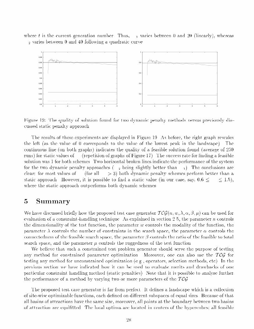
The results of these experiments are displayed in Figure 19. As before, the right graph rescalesthe left (as the value of 0 corresponds to the value of the lowest peak in the landscape). Thecontinuous line (on both graphs) indicates the quality of a feasible solution found (average of 250runs) for static values of W (repetition of graphs of Figure 17). The success rate for �nding a feasiblesolution was 1 for both schemes. Two horizontal broken lines indicate the performance of the systemfor the two dynamic penalty approaches (W2 being slightly better than W1). The conclusions areclear: for most values of W (for all W > 3) both dynamic penalty schemes perform better than astatic approach. However, it is possible to �nd a static value (in our case, say, 0:6 � W � 1:5),where the static approach outperforms both dynamic schemes.

5 Summary

We have discussed brie y how the proposed test case generator T CG(n;w; �; �; �; �) can be used forevaluation of a constraint-handling technique. As explained in section 2.5, the parameter n controlsthe dimensionality of the test function, the parameter w controls the modality of the function, theparameter � controls the number of constraints in the search space, the parameter � controls theconnectedness of the feasible search space, the parameter � controls the ratio of the feasible to totalsearch space, and the parameter � controls the ruggedness of the test function.

We believe that such a constrained test problem generator should serve the purpose of testingany method for constrained parameter optimization. Moreover, one can also use the T CG fortesting any method for unconstrained optimization (e.g., operators, selection methods, etc). In theprevious section we have indicated how it can be used to evaluate merits and drawbacks of oneparticular constraint handling method (static penalties). Note that it is possible to analyse furtherthe performance of a method by varying two or more parameters of the T CG.

The proposed test case generator is far from perfect. It de�nes a landscape which is a collectionof site-wise optimizable functions, each de�ned on di�erent subspaces of equal sizes. Because of thatall basins of attractions have the same size, moreover, all points at the boundary between two basinsof attraction are equi�tted. The local optima are located in centers of the hypercubes; all feasible

28

regions are centered around the local optima. Note also, that while we can change the number ofconstraints, there is precisely one (for �beta > 0) active constraint at the global optimum.

Some of these weaknesses can be corrected easily. For example, in order to avoid the thesymmetry and equal-sized basin of attraction of all subspaces, we may modify the T CG in thefollowing two ways. First, the parameter vector ~x may be transformed into another parametervector ~y using a non-linear mapping ~y = g(~x). The mapping function may be chosen in a way soas to have the lower and upper bounds of each parameter yi equal to zero and one, respectively.Such a non-linear mapping will make all subspaces of di�erent size. Second, in order to make thefeasible search space asymmetric, the center of each subspace for the outer hyper-sphere can bemade di�erent from that of the inner hyper-sphere. The following update of the center for the outerhyper-sphere can be used:

pki =�lki + uki

�=2 + ki �

ki ,

where �ki is a small number denoting the maximum di�erence allowed between centers of inner andouter hyper-spheres, and ki is a random number between zero and one. To avoid using anothercontrol parameter, �ki can be assumed to be the same for all subspaces. This modi�cation makesthe feasible search space asymmetric, although the maximum at each subspace remains the sameas in the original function.

It might be worthwhile to modify further the T CG to parametrize the number of active con-straints at the optima. It seems necessary to introduce a possibility of a more gradual incrementof the number of peaks. In the current version of the test case generator, w = 1 implies one peak,and w = 2 implies 2n peaks (this was the reason for using low values for parameter n). Also, thedi�erence between the lowest and the highest values of the peaks in the search space are, in thepresent model, too small.

All these limitations of the T CG diminish its signi�cance for being a useful tool for modelingreal-world problems, which may have quite di�erent characteristics. Note also, that it is necessaryto develop an additional tool, which would map a real-world problem into a particular con�gurationof the test case generator. In such a case, the test case generator should be able to \recommend"the most suitable constraint-handling method.

However, the proposed T CG is even in its current form an important tool for analysing anyconstraint-handling method in nonlinear programming (for any algorithm: not necessarily evolu-tionary algorithm), and it represents an important step in the \right" direction. The web pagehttp://www.daimi.au.dk/ marsch/TCG.html contains two �les: the T CG �le TCG.c (standard C),and TestTCG.c: an example �le that shows how to use the T CG.

Acknowledgments

The second author acknowledges the support provided by the Alexander von Humboldt Foundation,Germany. The research reported in this paper was partially supported by the ESPRIT Project 20288Cooperation Research in Information Technology (CRIT-2): \Evolutionary Real-time OptimizationSystem for Ecological Power Control".

References

B�ack, T., F. Ho�meister, and H.-P. Schwefel (1991). A survey of evolution strategies. In R. K. Belewand L. B. Booker (Eds.), Proceedings of the 4th International Conference on Genetic Algorithms,

29

pp. 2{9. Morgan Kaufmann.

B�ack, T. and M. Sch�utz, (1996). Intelligent Mutation Rate Control in Canonical Genetic Algorithms.In Z.W. Ras and M. Michalewicz (Eds.), Proceedings of the 9th International Symposium onMethodologies of Intelligent Systems, Springer-Verlag.

Bean, J. C. and A. B. Hadj-Alouane (1992). A dual genetic algorithm for bounded integer pro-grams. Technical Report TR 92-53, Department of Industrial and Operations Engineering, TheUniversity of Michigan.

Bilchev, G. and I. Parmee (1995). Ant colony search vs. genetic algorithms. Technical report, Ply-mouth Engineering Design Centre, University of Plymouth.

Colorni, A., M. Dorigo, and V. Maniezzo (1991). Distributed optimization by ant colonies. InProceedings of the First European Conference on Arti�cial Life, Paris. MIT Press/BradfordBook.

Davis, L. (1989). Adapting operator probabilities in genetic algorithms. In J. D. Scha�er (Ed.), Pro-ceedings of the 3rd International Conference on Genetic Algorithms, pp. 61{69. Morgan Kauf-mann.

Davis, L. (1997). Private communication.

Deb, K. (1995). Optimization for engineering design: Algorithms and examples. New Delhi:Prentice-Hall.

Deb, K. (in press). An e�cient constraint handling method for genetic algorithms. Computer Meth-ods in Applied Mechanics and Engineering.

DeJong, K. (1975). The Analysis of the Behavior of a Class of Genetic Adaptive Systems. Ph. D.thesis, University of Michigan, Ann Harbor. Dissertation Abstract International, 36(10), 5140B.(University Micro�lms No 76-9381).

Eiben, A., P.-E. Raue, and Z. Ruttkay (1994). Genetic algorithms with multi-parent recombination.In Y. Davidor, H.-P. Schwefel, and R. Manner (Eds.), Proceedings of the 3rd Conference onParallel Problems Solving from Nature, Number 866 in LNCS, pp. 78{87. Springer Verlag.

Eiben, A. and Z. Ruttkay (1996). Self-adaptivity for Constraint Satisfaction: Learning PenaltyFunctions. In Proceedings of the 3rd IEEE Conference on Evolutionary Computation, IEEEPress, 1996, pp. 258{261.

Eshelman, L. and J. D. Scha�er (1993). Real-coded genetic algorithms and interval-schemata. InL. D. Whitley (Ed.), Foundations of Genetic Algorithms 2, Los Altos, CA, pp. 187{202. MorganKaufmann.

Floudas, C. and P. Pardalos (1987). A Collection of Test Problems for Constrained Global Opti-mization Algorithms, Volume 455 of LNCS. Berlin: Springer Verlag.

Gregory, J. (1995). Nonlinear Programming FAQ, Usenet sci.answers. Available atftp://rtfm.mit.edu/pub/usenet/sci.answers/nonlinear-programming-faq.

Hadj-Alouane, A. B. and J. C. Bean (1992). A genetic algorithm for the multiple-choice integerprogram. Technical Report TR 92-50, Department of Industrial and Operations Engineering,The University of Michigan.

Himmelblau, D. (1992). Applied Nonlinear Programming. McGraw-Hill.

30

Hock, W. and K. Schittkowski (1981). Test Examples for Nonlinear Programming Codes, Volume187 of Lecture Notes in Economics and Mathematical Systems. Springer Verlag.

Homaifar, A., S. H.-Y. Lai, and X. Qi (1994). Constrained optimization via genetic algorithms.Simulation 62 (4), 242{254.

Joines, J. and C. Houck (1994). On the use of non-stationary penalty functions to solve nonlinearconstrained optimization problems with gas. In Z. Michalewicz, J. D. Scha�er, H.-P. Schwefel,D. B. Fogel, and H. Kitano (Eds.), Proceedings of the First IEEE International Conference onEvolutionary Computation, pp. 579{584. IEEE Press.

Keane, A.J. (1996). A Brief Comparison of Some Evolutionary Optimization Methods. In V.Rayward-Smith, I. Osman, C. Reeves and G. D. Smith (Eds.), Modern Heuristic Search Methods,J. Wiley, pp. 255{272.

Kelly, J. and M. Laguna (1996, April 8). Genetic Algorithms Digest. V10n16.

Kozie l, S. (1997). Evolutionary algorithms in constrained numerical optimization problems on con-vex spaces. Electronics and Telecommunications Quarterly, 43 (1), pp. 5{18.

Kozie l, S. and Z. Michalewicz, (1998). A decoder-based evolutionary algorithm for constrainedparameter optimization problems. In Proceedings of the 5th Conference on Parallel ProblemsSolving from Nature. Springer Verlag.

Kozie l, S. and Z. Michalewicz, (1999). Evolutionary Algorithms, Homomorphous Mappings, andConstrained Parameter Optimization. to appear in Evolutionary Computation.

Leriche, R. G., C. Knopf-Lenoir, and R. T. Haftka (1995). A segragated genetic algorithm forconstrained structural optimization. In L. J. Eshelman (Ed.), Proceedings of the 6th InternationalConference on Genetic Algorithms, pp. 558{565.

Maa, C. and M. Shanblatt (1992). A two-phase optimization neural network. IEEE Transactionson Neural Networks 3 (6), 1003{1009.

Michalewicz, Z. (1995a). Genetic algorithms, numerical optimization and constraints. In L. J. Eshel-man (Ed.), Proceedings of the 6th International Conference on Genetic Algorithms, pp. 151{158.Morgan Kaufmann.

Michalewicz, Z. (1995b). Heuristic methods for evolutionary computation techniques. Journal ofHeuristics 1 (2), 177{206.

Michalewicz, Z. (1995c). A Survey of Constraint Handling Techniques in Evolutionary ComputationMethods. Proceedings of the 4th Annual Conference on Evolutionary Programming, MIT Press,Cambridge, MA.

Michalewicz, Z. (1996). Genetic Algorithms+Data Structures=Evolution Programs. New-York:Springer Verlag. 3rd edition.

Michalewicz, Z. and N. Attia (1994). Evolutionary optimization of constrained problems. In Proceed-ings of the 3rd Annual Conference on Evolutionary Programming, pp. 98{108. World Scienti�c.

Michalewicz, Z., D. Dasgupta, R.G. Le Riche, and M. Schoenauer (1996). Test-case Generator forConstrained Parameter Optimization Techniques. Proceedings of EUROGEN'99, May 30 { June3, 1999, Jyv�askyl�a, Finland.

31

Michalewicz, Z., D. Dasgupta, R.G. Le Riche, and M. Schoenauer (1996). Evolutionary Algorithmsfor Constrained Engineering Problems. Computers & Industrial Engineering Journal, Vol.30,No.2.

Michalewicz, Z., Deb, K., Schmidt, M., and Stidsen, T. (1999a). Evolutionary Algorithms for En-gineering Applications. Proceedings of the EUROGEN'99, May 30 { June 3, 1999, Jyv�askyl�a,Finland.

Michalewicz, Z., Deb, K., Schmidt, M., and Stidsen, T. (1999b). Towards Understanding Constraint-Handling Methods in Evolutionary Algorithms. Submitted for publication.

Michalewicz, Z. and C. Z. Janikow (1991). Handling constraints in genetic algorithms. In R. K.Belew and L. B. Booker (Eds.), Proceedings of the 4th International Conference on GeneticAlgorithms, pp. 151{157. Morgan Kaufmann.

Michalewicz, Z., T. Logan, and S. Swaminathan (1994). Evolutionary operators for continuousconvex parameter spaces. In Proceedings of the 3rd Annual Conference on Evolutionary Pro-gramming, pp. 84{97. World Scienti�c.

Michalewicz, Z. and M. Michalewicz (1995). Pro-Life versus Pro-Choice Strategies in EvolutionaryComputation Techniques. Chapter 10 in Evolutionary Computation, IEEE Press.

Michalewicz, Z. and G. Nazhiyath (1995). Genocop III: A co-evolutionary algorithm for numericaloptimization problems with nonlinear constraints. In D. B. Fogel (Ed.), Proceedings of the SecondIEEE International Conference on Evolutionary Computation, pp. 647{651. IEEE Press.

Michalewicz, Z., G. Nazhiyath, and M. Michalewicz (1996). A note on usefulness of geometricalcrossover for numerical optimization problems. In P. J. Angeline and T. B�ack (Eds.), Proceedingsof the 5th Annual Conference on Evolutionary Programming.

Michalewicz, Z. and M. Schoenauer (1996). Evolutionary computation for constrained ParameterOptimization Problems. Evolutionary Computation, Vol.4, No.1, pp.1{32.

M�uhlenbein, H. and H.-M. Voigt (1995). Gene pool recombination for the breeder genetic algorithm.In Proceedings of the Metaheuristics International Conference, pp. 19{25.

Myung, H., J.-H. Kim, and D. Fogel (1995). Preliminary investigation into a two-stage method ofevolutionary optimization on constrained problems. In J. R. McDonnell, R. G. Reynolds, andD. B. Fogel (Eds.), Proceedings of the 4th Annual Conference on Evolutionary Programming, pp.449{463. MIT Press.

Orvosh, D. and L. Davis (1993). Shall we repair? Genetic algorithms, combinatorial optimization,and feasibility constraints. In S. Forrest (Ed.), Proceedings of the 5th International Conferenceon Genetic Algorithms, pp. 650. Morgan Kaufmann.

Palmer, C.C. and A. Kershenbaum (1994). Representing Trees in Genetic Algorithms. In Proceedingsof the IEEE International Conference on Evolutionary Computation, 27{29 June 1994, 379{384.

Paredis, J. (1994). Coevolutionary constraint satisfaction. In Y. Davidor, H.-P. Schwefel, andR. Manner (Eds.), Proceedings of the 3rd Conference on Parallel Problems Solving from Na-ture, pp. 46{55. Springer Verlag.

Parmee, I. and G. Purchase (1994). The development of directed genetic search technique for heavilyconstrained design spaces. In Proceedings of the Conference on Adaptive Computing in Engineer-ing Design and Control, pp. 97{102. University of Plymouth.

32

Powell, D. and M. M. Skolnick (1993). Using genetic algorithms in engineering design optimizationwith non-linear constraints. In S. Forrest (Ed.), Proceedings of the 5th International Conferenceon Genetic Algorithms, pp. 424{430. Morgan Kaufmann.

Rechenberg, I. (1973). Evolutionstrategie: Optimierung Technisher Systeme nach Prinzipien desBiologischen Evolution. Stuttgart: Fromman-Holzboog Verlag.

Renders, J.-M. and H. Bersini (1994). Hybridizing genetic algorithms with hill-climbing methodsfor global optimization: Two possible ways. In Z. Michalewicz, J. D. Scha�er, H.-P. Schwefel,D. B. Fogel, and H. Kitano (Eds.), Proceedings of the First IEEE International Conference onEvolutionary Computation, pp. 312{317. IEEE Press.

Reynolds, R. (1994). An introduction to cultural algorithms. In Proceedings of the 3rd AnnualConference on Evolutionary Programming, pp. 131{139. World Scienti�c.

Reynolds, R., Z. Michalewicz, and M. Cavaretta (1995). Using cultural algorithms for constrainthandling in Genocop. In J. R. McDonnell, R. G. Reynolds, and D. B. Fogel (Eds.), Proceedingsof the 4th Annual Conference on Evolutionary Programming, pp. 298{305. MIT Press.

Richardson, J. T., M. R. Palmer, G. Liepins, and M. Hilliard (1989). Some guidelines for geneticalgorithms with penalty functions. In J. D. Scha�er (Ed.), Proceedings of the 3rd InternationalConference on Genetic Algorithms, pp. 191{197. Morgan Kaufmann.

Rudolph, G. (1996). Convergence properties of evolutionary algorithms. Hamburg: Verlag Dr. Ko-vacheckc.

Scha�er, D. (1985). Multiple objective optimization with vector evaluated genetic algorithms. InJ. J. Grefenstette (Ed.), Proceedings of the 1st International Conference on Genetic Algorithms.Laurence Erlbaum Associates.

Schoenauer, M. and Z. Michalewicz (1996). Evolutionary computation at the edge of feasibility. W.Ebeling, and H.-M. Voigt (Eds.), Proceedings of the 4th Conference on Parallel Problems Solvingfrom Nature, Springer Verlag.

Schoenauer, M. and Z. Michalewicz (1997). Boundary Operators for Constrained Parameter Opti-mization Problems. In T. B�ack (Ed.), Proceedings of the 7th International Conference on GeneticAlgorithms, pp.320{329. Morgan Kaufmann.

Schoenauer, M. and S. Xanthakis (1993). Constrained GA optimization. In S. Forrest (Ed.), Proceed-ings of the 5th International Conference on Genetic Algorithms, pp. 573{580. Morgan Kaufmann.

Schwefel, H.-P. (1981). Numerical Optimization of Computer Models. New-York: John Wiley &Sons. 1995 { 2nd edition.

Smith, A. and D. Tate (1993). Genetic optimization using a penalty function. In S. Forrest (Ed.),Proceedings of the 5th International Conference on Genetic Algorithms, pp. 499{503. MorganKaufmann.

Surry, P., N. Radcli�e, and I. Boyd (1995). A multi-objective approach to constrained optimiza-tion of gas supply networks. In T. Fogarty (Ed.), Proceedings of the AISB-95 Workshop onEvolutionary Computing, Volume 993, pp. 166{180. Springer Verlag.

van Kemenade, C.H.M. (1998). Recombinative evolutionary search. PhD Thesis, Leiden University,Netherlands, 1998.

33

Waagen, D., P. Diercks, and J. McDonnell (1992). The stochastic direction set algorithm: A hybridtechnique for �nding function extrema. In D. B. Fogel and W. Atmar (Eds.), Proceedings of the1st Annual Conference on Evolutionary Programming, pp. 35{42. Evolutionary ProgrammingSociety.

Whitley, D., K. Mathias, S. Rana, and J. Dzubera (1995). Building better test functions. In L.Eshelmen (Editor), Proceedings of the 6th International Conference on Genetic Alforithms,Morgam Kaufmann, 1995.

Whitley, D., K. Mathias, S. Rana, and J. Dzubera (1995). Evaluating evolutionary algorithms.Arti�cial Intelligence Journal, Vol.85, August 1996, pp.245{276.

Wodrich, M. and G. Bilchev (1997). Cooperative distributed search: the ant's way. Control &Cybernetics, 26 (3).

Wright, A. (1991). Genetic algorithms for real parameter optimization. In J. G. Rawlins (Ed.),Foundations of Genetic Algorithms, pp. 205{218. Morgan Kaufmann.

34