UNCERTAINTY IN THE RAINFALL INPUT DATA IN A CONCEPTUAL WATER

BALANCE MODEL: . EFFECTS ON OUTPUTS AND IMPLICANCES IMPLICATIONS

ON THE PREDICTABILITY

Enrique Muñoz, Pedro Tume, Gabriel Ortíz1

ABSTRACT

As the use of hHydrological models have been widely used in the water resroucesresources

planning and management of water resourceshas become more prevalent, , an increasing level of

detail and precision has been demanded of them. and therefore the model capabilities and

limitations have become highly which are being more exploited. in terms of their capabilities and

limitations. Currently, it is not only proves indispensable to have reliable models that simulate the

hydrological behavior of a basin, but it is also necessary to know the limits of predictability and

confiability reliability of the model outputs. The present study evaluates the influence on output

uncertainty in a hydrological model produced by uncertainty in the main input variable of the

model, rainfall. Using concepts ofTo do this, using concepts of identifiability and sensitivity, the

uncertainty of model structure and parameters uncertainty associated with the model structure

and calibration parameters was werewas estimated. Then, the output uncertainty , and then, using

this foundation, the influence on the outputs produced by uncertainty in caused by uncertainties

in i) the rainfall amounts, and ii) the periods of occurrence of these amounts, was determined.

Among tThe main conclusions isconclusion is that the model presented greater sensitivity to

1Alonso de Ribera 2850, Concepción. Departamento de Ingeniería Civil, Universidad Católica de la Santísima Concepción, Concepción, Chile - mail: emunozo@ucsc.cl, ptume@ucsc.cl, gaortiz@ing.ucsc.cl

1

1

2

3

4

5

6

7

8

9

10

11

12

13

14

15

16

17

18

19

20

21

22

12

rainy periods, and therefore, greater uncertainty in rainfall the estimation of rainfall during rainy

periods produces a greater output uncertainty in the outputs. On the other hand, in non-rainy

periods, the output uncertainty bands are not very sensitive to uncertainty in rainfall. Finally, , is

was determined that uncertainties in rainfall during the basin filling and emptying periods (Apr. –

. to Jun., and Sep. to – Nov., respectively) produce an alteration in the uncertainty bands in theof

subsequent periods. Therefore, uncertainties in these periods could result in limited , increasing

the average range of uncertainty of the model outputs, and limiting the ranges of model

predictabilityility. of the model.

Key words: Uncertainty, hydrological predictability, surface hydrology, conceptual water

balance model, water resources.

INTRODUCTION

Considering that i) water is a limited resource, that ii) demand for it increases with development

and population growth, that iii) availability changes year to year due to local, global, natural and

anthropogenic phenomena, that iv) the impact of climate change on the water supply is of

fundamental importance, and that v) a large part of the world population is already experiencing

water stress (Vörösmarty et al., 2000), it is necessary to develop tools that allow for an efficient

water resources management and to of water resources and that support the prediction of future

conditions under different scenarios caused by local (orographic), regional (El Niño Southern

Oscillation) or global effects (climate change), in order to avoid or reduce water stress in basins

around the world..

2

23

24

25

26

27

28

29

30

31

32

33

34

35

36

37

38

39

40

41

42

43

44

45

One alternative for the efficient water resources management and planning of water resources is

the use of hydrological models. A model attempts to reproduce a physical phenomenon that

occurs in an object or area. Therefore, in hydrology, a model seeks to represent an area defined

by a watershed, the phenomenaon of rainfall-runoff processes and the water movement within

itthem. The object objective of reproducing these processes is to simulate and predict future

conditions with the aim of acting from a perspective of management, administration and

optimization of water uses.

Consequently, it not only proves essential not only to have reliable models that adequately

represent the hydrological behavior of a basin, but also, in the . For example, in case of using

predictive models, or the use of using alternative sources of information (for example using

climatological databases interpolated at a global or regional scale as hydrological modele.g global

datasets inputs) (Mahe et al., 2008, Muñoz, 2010), proves it is necessary to know the

predictability limits of the model outputs, and the uncertainty associated with them.

Normally, a hydrological conceptual hydrological model requires at least two input variables

(potential evapotranspiration and rainfall) in order to quantify the inputs and water losses in the

water balance. It is known that rainfall is the main input variable in a hydrological model (Olsson

and Lindström, 2008). T, and therefore, the potential predictability and the range of predictability

of the basin flows will depend on the uncertainty associated with the input variables and their

quality, and on the uncertainty produced by the model..

Uncertainty is defined as the degree of the lack of knowledge of or confidence in a certain

process or result (Caddy and Mahorn, 1995). Therefore, in a hydrological model the sources of

uncertainty are associated with the input variables (lack of knowledge of the quality of the

measurements and predictions) and with the model structure and calibration parameters (lack of

knowledge and simplification of the simulated hydrological processes in a basin).

3

46

47

48

49

50

51

52

53

54

55

56

57

58

59

60

61

62

63

64

65

66

67

68

69

The present study aims to quantify how uncertainty in the outputs of a conceptual hydrological

model is affected by uncertainty in the main input, the rainfall, while keeping fixed the

uncertainty associated with the model structure and calibration parameters fixed, in order to

discuss and evaluate the implications on the confiability and hydrological predictability of the

model outputs..

MATERIALS AND METHODS

Study Case Study

For the study case, a conceptual water balance model of the Polcura River Basin was constructed

(Figure 1).

The Polcura River Basin (Figure 1) is located in the temperate zone of South-Central Chile,

between 37°20'S - 71º31'W and 36°54'S - 71°06'W. It is bounded by the Andes on the East, the

Nevados de Chillán volcanic complex on the southnorth, and Lake Laja on the northsouth. It

comprises an area of 914 km2 between 700 and 3,090 masl, and it is characterized by steep

slopes (≈ 26° on average) and is mainly composed of partially eroded volcano-sedimentary

sequences partially eroded (OM2c, PPl3 and M3i) (SERNAGEOMIN, 2006).

. In addition, it is located in one of the extratropical zones most affected by the El Niño Southern

Oscillation phenomenon (ENSO) (Grimm et al., 2000), presenting interannual seasonality and

interannual variability in the local hydro-meteorological patterns (Grimm et al., 2000;,

Montecinos and Aceituno, 2003).

4

70

71

72

73

74

75

76

77

78

79

80

81

82

83

84

85

86

87

88

89

90

91

The average annual precipitation in the basin is 2300 mm with a pluvial period during winter and

aan ice-melt and snow-melt period in spring and the start of summer. The average monthly

temperature is 9° C, and ranges from 2.5° C in winter to 16.5 ° C in summer.

Due to the location of the basin, its mountainous nature, and its geomorphology (Figure 1), it it

presents exhibits high temporal variability with respect to hydro-meteorological characteristics,

where the orographic effect on the eastern slope of the Andes produces an increase in rainfall

amounts (Garreaud, 2009;, Vicuña et al., 2011). Additionally, it is a zone affected by the ENSO

phenomenon. ENSO is a coupled ocean-atmosphere phenomenon that is characterized by

irregular periodicity (2 to 7 years), where the alternation between El Niño and La Niña is the

main source of interannual variability, where El Niño/La Niña episodes are is associated with

above/below average rainfall and warmer/colder than normal air temperature warmer/colder than

normal (Garreaud, 2009).

Therefore, due to the characteristics of the basin characteristics such as high rainfall variability

and ENSO influence result in an ideal case of study where in which uncertainty in precipitation

could be the main source of uncertainty in predictions.

ConceptualDescription of the water balance model description

The model used in this paper is the snow-rain and semi-distributed conceptual water balance

model presented in Muñoz (2010) and Muñoz et al. (2011). This model simulates the pluvial and

snow-melting processes separately and includes external alterations such as irrigation or transfer

canals by adding or subtracting flows. This model has been successfully implemented in Andean

basins in south-central Chile (e.g. Zúñiga et al., 2012, Arumí et al., 2012). Therefore, it is an

adequate option tofor analyzing e the study area.

5

92

93

94

95

96

97

98

99

100

101

102

103

104

105

106

107

108

109

110

111

112

113

114

115

The pluvial component is modeled through a lumped monthly rainfall-runoff model that

considers the watershed as a double storage system: the subsurface-superficial (SS) and the

underground storage (US). The SS represents the water stored into the unsaturated soil layer as

soil moisture. The US is the water that covers the saturated soil layer. The model needs requires

two inputs, rainfall (PM) and potential evapotranspiration (PET). The model output is the total

runoff (ETOT) at the watershed outlet, and includes both the subterraneaneous (ES) and direct

runoff (EI). These , whose amounts are calculated through six calibration parameters of

calibration, plus two for the input modification (useful in case of non-representative PM and PET

data).

The snow-melt model calculates the snowfall (Psnow) based on the rainfall precipitation above

the 0 (°C) isotherm. Psnow is stored in the snow storage system (SN), on which the melting

calculations are performed based on the concept ofusing the degree-day method (Rango and

Martinec, 1995). Thus, the potential melting (PSP) is estimated, and then based depending on the

snow stored,; the real melting (PS) is calculated. LaterThen, PS is distributed into the pluvial

model through the calibration the parameter of calibration F.

Every calibration parameter of calibration has a conceptual physical meaning, integrating spatial

and temporal variability. Table 1 presents a brief description of the model parameters and their

influence on the model.

The external alterations module permits the incorporation of alterations such as irrigation or

transfer canals, and simulates inflows and/or outflows to/from the basin by adding or subtracting

flows as follows:

6

116

117

118

119

120

121

122

123

124

125

126

127

128

129

130

131

132

133

134

135

136

137

138

Qout (t )=ETOT ( t )+Qcontributions ( t )−Qextractions (t ) (1)

Where the basin outflow (Qout) at the time t, is the basin runoff (ETOT) plus the contributions

(Qcontributions) and less the extractions (Qextractions) during the same period.

For a further explanation of the model, refer to Muñoz (2010) and Muñoz et al. (2013)..

Model inputs

In order to run the described model, it is necessary to have precipitation, temperature and

potential evapotranspiration series, as well as the geomorphological characterization of the basin

to allow compute the monthly 0°C isotherm elevation.

For the geomorphological characterization of the basin, a digital elevation model was constructed

using data from the Shuttle Radar Topography Mission (SRTM) of 3 arc-seconds (90 m). Fort the

inputs, rainfall series from the pluviometric rain gauge stations Las Trancas, San Lorenzo and

Trupán were obtained (administrated by the Dirección General de Aguas, DGA), and synthetic

temperature series from the Center for Climatic Research of the University of Delaware (UD) (,

Willmot and Matsuura, 2008) were collected. Then the cClimatological model inputs were

constructed using both sources of information. Additionally, the potential evapotranspiration

series was were calculated using the Thornthwaite method and UD temperature data series. The

spatial distribution of said these variables in the basin was carried out through Thiessen polygons.

Based on prior experiences, both, the Thornthwaite and Thiessen polygons methods have been

demonstrated to be adequate for estimating potential evapotranspiration and for meteorological

spatial distribution of monthly data in basins of south-central Chile (e.g. Muñoz, 2010, Zúñiga et

al., 2012). Therefore, both methods were used in this study.

7

139

140

141

142

143

144

145

146

147

148

149

150

151

152

153

154

155

156

157

158

159

160

161

Due to the availability and quality of the input data, the analysis was performed on a monthly

time-step for a period of 13 years (1990 – 2002). The fluviometric stream gauge station for

controlling the basin outflows was is Polcura Antes de Descarga central El Toro station (Figure

1).

Uncertainty analysis

In order to quantify the uncertainty, the Monte Carlo Analysis Toolbox (MCAT) (, Wagener and

Kollat, 2007) was used. MCAT is a tool that operates under the Generalized Likelihood

Uncertainty Estimation methodology (Beven and Binley, 1992) and contains a group of analysis

tools that allowto explore the identifiability of a model and its parameters to be investigated,

where a . well-identified model is considered a model with realistic behavior (Wagener et al.,

2001).MCAT was usedchosen because it is an easy-ofto-use tool and is an adequate and simple

option tofor evaluateing model behavior and uncertainty.

In order to evaluate identifiability and quantify the uncertainty of a model, MCAT operates by

performing repetitive simulations using a set of randomly selected parameters within a range

defined by the user. . The program stores the outputs and values of the objective function(s) for

posterior subsequent analyses. In this case, due to the lack of knowledge about the parameter

distribution, a prior uniform distribution of the model parameters was used.

Parameters of hydrological models cannot be identified as unique sets of values. This is mainly

due to the fact thatbecause changes of one parameter can be compensated for by changes of one

or more others due to their interdependence (Bárdossy, 2007), and due to thebecause fact that the

processes simulated in a hydrological model are commonly interrelated. In the case of the Muñoz

(2010) model it is held, for example, that the direct runoff depends on Cmax, and therefore the

processes that occur in the subsurface storage layer depend on the amount of rainfall that is not

8

162

163

164

165

166

167

168

169

170

171

172

173

174

175

176

177

178

179

180

181

182

183

184

185

transformed into runoff, that is, on 1-Cmax, and consequently the processes that occur in saidthis

storage layer will depend on the identifiability of Cmax. This generates an interconnection

betweenamong the identifiability of the calibration parameters of a model. Therefore, it proves

necessary to perform various iterations as a means of restricting the range of validity of the

parameters that first show identifiability, in order to then observe identifiability in the remaining

(dependent) parameters as a means of also reducing the range of identifiability of these

parameters.

Because the Monte Carlo method is based on random trials, it normally requires a large number

of simulations to cover a wide spectrum of possible simulations. In this case, the number of

Monte Carlo simulations was estimated via trial and error, where the stop criterion was met when

the correlation (according to the Pearson correlation coefficient) between uncertainty bands

(calculated as a linear correlation between the time-series of the upper and lower limits of the

bands of uncertainty bands) of two different trials, but with same number of simulations, was

equal to or greater than 0.999. Under this criterion, it was determined that the adequate number of

simulations for this study is 25,000.

The processes simulated in a hydrological model are normally interrelated. In the case of the

Muñoz (2010) model it is seen, for example, that the direct runoff depends on Cmax, and

therefore the processes that occur in the subsurface storage layer will depend on the amount of

rainwater that does not become runoff, which is to say, on 1-Cmax, and consequently, the

processes that occur in said storage layer will depend on the identifiability of Cmax. This

generates an interconnection among the identifiability of the calibration parameters of a model.

Therefore, it proves necessary to perform various iterations as a means of restricting the range of

validity of the parameters that first show identifiability, in order to then observe identifiability in

9

186

187

188

189

190

191

192

193

194

195

196

197

198

199

200

201

202

203

204

205

206

207

208

the remaining (dependent) parameters, thereby also reducing the range of identifiability of these

parameters.

In the present study, in order to quantify the uncertainty associated with rainfall, 25000

simulations were performed, from which, first, the uncertainty associated with the calibration

parameters and model structure, was determined, and then the effect on this uncertainty due to a

given uncertainty in rainfall, were determined. The procedure to estimate the rainfall uncertainty

and to differentiate it from model structure used and calibration parameters was the as

followingfollows:

i) i) throughThrough an identifiability analysis of the factors for the modification of the

inputs (a comparison of these factors with the value of the objective function), these

factors were limited to precise values. It provesisIt is necessary to set these factors to a

unique value, as they fulfill the function of assuring the closure of the long-term water

balance, assuring that the precipitation input volumes are equal to the

evapotranspiration and flow output volumes during the entire period of the simulation.

ii) , and ii) withWith the values of said thoese fixed factors, new simulations were

performed, in which the ranges of variation assigned to each parameter were reduced

in accord with the observed identifiability. The established stop criterion was when

identifiability was not observed in the new defined range (the reduced range) of each

parameter.

After the identifiability analysis, the resulting uncertainty in the model outputs was quantified.

This uncertainty was defined as the uncertainty associated with the model structure and

calibration parameters.

The confidence level used was 90% (a range between 5 and 95% of the outputs for each time-step

of the series). The established rejection criterion was set according to the Kling-Gupta efficiency

10

209

210

211

212

213

214

215

216

217

218

219

220

221

222

223

224

225

226

227

228

229

230

231

232

objective function (KGE) (, Gupta et al., 2009). The KGE function (Eq. 2) is an improvement of

the Nash-Suctliffe efficiency index (NSE) (, Nash and Sutcliffe, 1970) in which the correlation,

deviation and variability are equally weighted, resolving systematic problems of underestimation

of the maximum values and low variability identified in the NSE function (Gupta et al., 2009).

The KGE varies between −∞ to 1 where the betterst model is closerst to 1. Due toBecause the

GLUE methodology is based on likelihood, the KGE was transformed asinto 1-KGE. With this

change, the 1-KGE represents a measure of likelihood where the best model is closerst to 0 and

the worst model tends to +∞.

KGE=1−√ (r−1 )2+(α−1 )2 + (β−1 )2 (2)

Where r is the linear correlation between simulated and observed flows, α is the ration between

the standard deviation of simulated and observed flows, representing the variability in the values,

and β is the ratio between mean simulated and mean observed flows (i.e. represents the bias).

Then, with the uncertainty associated with the model structure and parameters quantified, the

rainfall series were modified in different magnitudes and periods, as shown in Table 2. It isIs

important to point out that this variation corresponds to a punctual variation of the rainfall series

in different magnitudes and periods, and the uncertainty is not added as a range of rainfall data in

each time-step. This analysis aims to identify how output uncertainty would be affected by an

error in the precipitation prediction.

RESULTS AND DISCUSSION

11

233

234

235

236

237

238

239

240

241

242

243

244

245

246

247

248

249

250

251

252

253

Using the previously described methods described before, uncertainty ofassociated with model

structure and parameters wereas found, and then the uncertainty related to rainfall data was

computed and analyzed. The major findings and a discussion is are presented as follows.

Uncertainty associated with model structure and calibration parameters

Figure 2 shows the identifiability and sensitivity analysis performed for each model calibration

parameters. Each gThe gGraphs shows the probability distribution function (pdf) and the

cumulative distribution function (cdf) of each parameter for the best 10% of the simulations

according to a determined objective function (KGE in this case).

Figure 2 showsAs is observed, five parameters that presented identifiability (according to the

pdf), A, B, Cmax, Hmax and Ck, of which (according to the cdf) A, Cmax and Ck prove to be the

most sensitive (greater slope within a determined range) to the model outputs.

As a result of the identifiability analysis From the previous analysis, the ranges of variation of

those these five identifiable model parameters were reduced. It is important to mention that aA

complementary analysis was performed, in which the value of each parameter versus the value of

the objective function was plotted, and based on this analysis, it was determined that the factor

that modifies the inputs (A) has an optimal value of 1.58. This means the differences between

simulated and observed flows according to the KGE are minimal when A is 1.58. This analysis

allows the value of said the parameter to be fixed and the influence of model structure and

parameters on output uncertainty to be separated from later analyses.

The resultanting value of parameter A suggests that the distributed rainfall over the basin was

underestimated. The underestimation is caused due to the orographic effect and itthe related

enhancement of rainfall in mountain areas (Garreaud, 2009), which is not well recorded by the

12

254

255

256

257

258

259

260

261

262

263

264

265

266

267

268

269

270

271

272

273

274

275

276

meteorological stations, mainly because they are located in the lower part of the basin under

study.

Finally, the aforementioned parameters were limited to the following ranges: i) B [1.2 – 1.7], ii)

Cmax [0.3 – 0.52], iii) Hmax [220 – 500], iv) Ck [0.25 – 0.52]. The remaining parameters, upon

presenting exhibiting neither greater sensitivity nor identifiability, were kept in the initial range

of the simulations.

Then, considering the aforementioned parameter ranges, and using MCAT, the output uncertainty

associated with the model structure and calibration parameters was estimated. Next, using this

data, the influence of the input variables on uncertainty in the outputs was estimated.

Uncertainty Associated with the Input Rainfall Data

By incorporating the variations in rainfall in accordance with Table 2, new ranges of uncertainty

were estimated. In order to identify them and observe the differences generated due to the

modification of the input variables, Figures 3 to 7 show the uncertainty bands associated with the

model structure and calibration parameters (white area between black lines), the uncertainty

associated with positive variations in rainfall (blue area), and the uncertainty associated with

negative variations in rainfall (red area). Also, in order to quantify said the propagation of rainfall

uncertainty effects, Table 3 presents a summary in which the average width of the uncertainty

bands is indicated (in m3/s) for the different variations in the rainfall data. Additionally, Table 4

presents the percentage of variations of said these ranges.

Figure 3 shows that the model outputs are sensitive to changes in the rainfall amounts, where the

range of uncertainty increases by an average of 15% for positive variations and 14% for negative

variations in rainfall (Table 4). Upon comparing said these results with Figure 3, it can be

observed that overestimations of rainfall amounts result in an increase in the uncertainty toward

13

277

278

279

280

281

282

283

284

285

286

287

288

289

290

291

292

293

294

295

296

297

298

299

300

greater flows, while underestimations of said rainfall amounts result in an increase inof the

uncertainty in the outputs toward greater and lesser flows.

Figure 4 shows that errors in the prediction of rainfall amounts during the winter period generate

an effect on the flows of the recession curve, increasing the range of uncertainty in the outputs of

the model in the spring-summer (Oct.-Feb.) and even the early fall period (Mar.-Apr.) (see

Figure 4 in the previous periods prior to the peak flows in Figure 4), and increasing the discharge

amounts estimated by the model.

Figure 5 shows that errors in the estimation of rainfall in summer do not significantly affect

uncertainty in the model outputs, probably because the earlier and later flows of the period

analyzed depend mainly on base flow and water storage in the basin during winter, and not on the

runoff that can be produced in summer.

Figure 6 shows that overestimations in the prediction of rainfall during the basin filling period

produce a displacement of the outputs uncertainty bands toward greater flows, but maintain a

relatively constant uncertainty band width (Tables 3 and 4). This result suggests a high sensitivity

of the model to overestimations of rainfall data in such a period, probably because the model is

not capable of redistributinge the water into the basin processes, and therefore higher flows

butand a similar width of uncertainty bands isare obtained. In contrast, underestimations of

rainfall in said this period do not result in greater differences in uncertainty band width,

suggesting that the uncertainty is related to different processes and/or parameters. such as for

example, the underground storage.

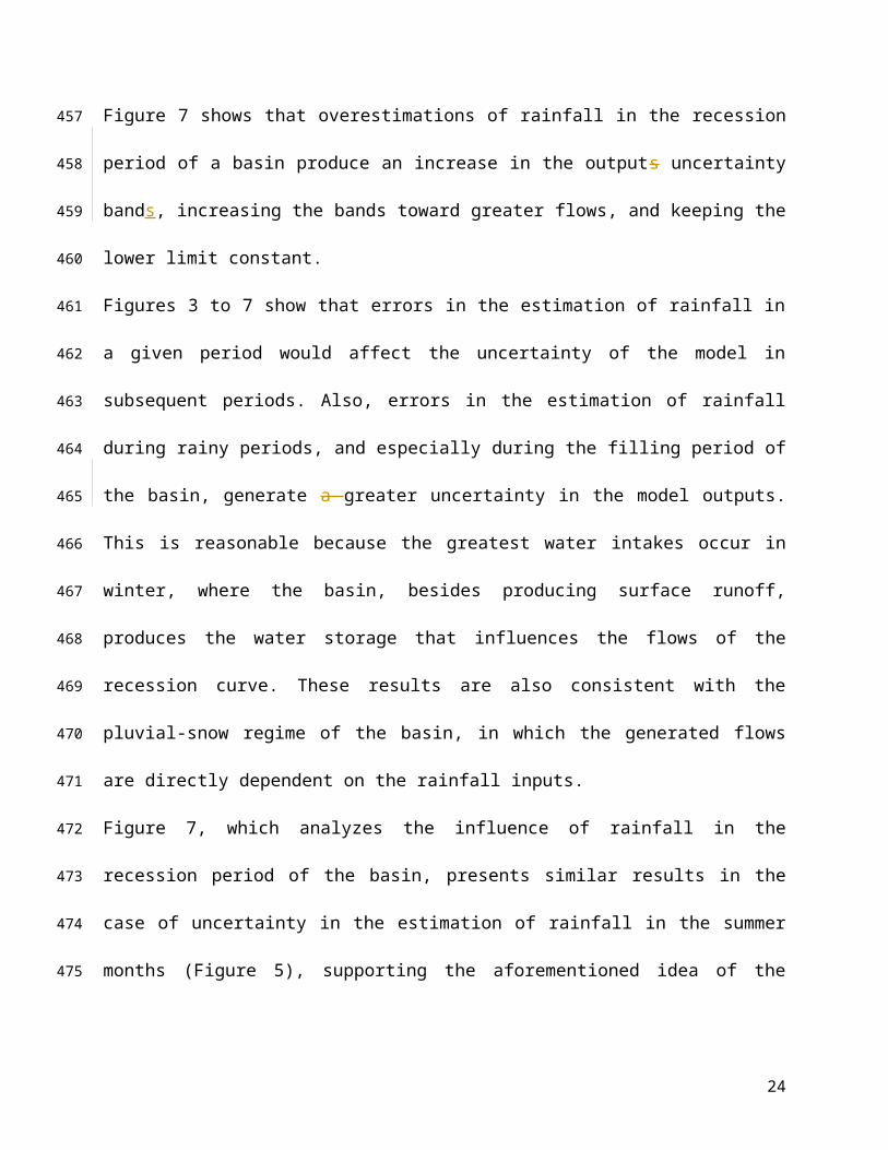
Figure 7 shows that overestimations of rainfall in the recession period of a basin produce an

increase in the outputs uncertainty bands, increasing the bands toward greater flows, and keeping

the lower limit constant.

14

301

302

303

304

305

306

307

308

309

310

311

312

313

314

315

316

317

318

319

320

321

322

323

Figures 3 to 7 show that errors in the estimation of rainfall in a given period would affect the

uncertainty of the model in subsequent periods. Also, errors in the estimation of rainfall during

rainy periods, and especially during the filling period of the basin, generate a greater uncertainty

in the model outputs. This is reasonable because the greatest water intakes occur in winter, where

the basin, besides producing surface runoff, produces the water storage that influences the flows

of the recession curve. These results are also consistent with the pluvial-snow regime of the

basin, in which the generated flows are directly dependent on the rainfall inputs.

Figure 7, which analyzes the influence of rainfall in the recession period of the basin, presents

similar results in the case of uncertainty in the estimation of rainfall in the summer months

(Figure 5), supporting the aforementioned idea of the existence of an important dependence of the

model and its outputs on the inputs of water to the basin in rainy periods.

Tables 3 and 4 show that the model structure and parameters generate a range of output

uncertainty of 13 (m3/s), on average. After estimating how model uncertainty is affected by an

uncertainty in the rainfall amounts during different periods, it is observed that the outputs prove

more sensitive to rainy periods, which is observed in greater ranges of uncertainty and greater

percentage changes in uncertainty bands. A smaller influence is observed for low water periods

(recession and summer) where the model outputs present lower sensitivity to errors or

uncertainties in the estimation of rainfall amounts. On the other hand, in the filling period of the

basin it is observed that the width of uncertainty bands does not increase significantly (8% on

average), but it is displaced toward greater flows when rainfall is overestimated.

15

324

325

326

327

328

329

330

331

332

333

334

335

336

337

338

339

340

341

342

343

344

345

346

347

CONCLUSIONS

The model has greater sensitivity to rainy periods, and therefore, a greater uncertainty in the

estimation of rainfall during said these periods directly influences uncertainty in the model

outputs, increasing the range of the related uncertainty bands.

The output uncertainty is highly sensitive to rainfall. In Therefore, in dry periods,, where in

which the rainfall amounts are relatively small, the model is less sensitive to uncertainties in

rainfall than in wet periods., without producing greater effects on the uncertainty bands of the

model outputs.

Currently, there is a tendency to estimate flows produced by a hydrological model along with the

uncertainty bands associated with said simulated flows. In the present study, it has been observed

that the uncertainty associated with the main water input (rainfall) in an Andean basin (rainfall)

can generate a significant increase in the uncertainty bands of the outputs. Therefore, in the case

ofwhen using alternative sources of information to feed a hydrological model (for examplee.g.

global gridded data or data interpolated at a global scale), it is necessary to reduce the uncertainty

associated with the predictions by ascertaining and reducinge the deviation of said rainfall data in

rainy periods (with respect to the real observed or ground values), as a means of reducing the

uncertainty associated with the predictions and/or ascertaining the quality of the presented

predictions. Also, if the use of afor predictive hydrological models is desired, a high uncertainty

in periods of low rainfall does not greatly influence the uncertainty in the outputs. ; hHowever, in

the case of prediction flows in rainy periods, or in recession periods of the basin, it is

recommendable recommended to evaluate the uncertainty associated with pluviometric

predictability before predicting flows, in order to estimate the influence on uncertainty associated

with the flows..

16

348

349

350

351

352

353

354

355

356

357

358

359

360

361

362

363

364

365

366

367

368

369

370

371

ACKNOWLEDGEMENTS

This research has been supported by the EU Erasmus Mundus External Cooperation Window, the

CONICYT “Programa Nacional de Formación de Capital Humano Avanzado” scholarship,

and the BMBF/CONICYT Project 2008099 “Impacto de la variabilidad climática en la

disponibilidad de recursos hídricos y requerimientos de riego en la Zona Central de Chile”.

The authors thank the Dirección General de Aguas for providing the rain gauge and fluviometric

stream gauge data.

LITERATURE CITEDREFERENCES

Arumí, J.L., D. Rivera, E. Muñoz, M. Billib. 2012. Interacciones aguas superficiales y

subterráneas en la zona central de Chile. Obras y Proyectos, 12, 4-13.

Bárdossy A., 2007. Calibration of Hydrological Model Parameters for Ungauged Catchments,

Hydrology and Earth System Sciences, 11(2), 703–710.

Beven, K., and Binley, A. (1992). The future of distributed models: model calibration and

uncertainty prediction. Hydrological Processes, 6, 279-298.

Caddy, J. and Mahor, R. (1995). Reference points for fisheries management. FAO Fisheries

Technical Paper, 346. Food and Agriculture Organization of United Nations, Rome, Italy.

Garreaud, R. D. (2009). The Andes climate and weather, Advances in Geosciences, 22, 3–11.

Grimm, A. M., Barros, V. R., and Doyle, M. E. (2000). Climate variability in southern South

America associated with El Niño and La Niña events, Journal of Climate, 13, 35-58.

17

372

373

374

375

376

377

378

379

380

381

382

383

384

385

386

387

388

389

390

391

392

393

Gupta, H. V., Kling, H., Yilmaz, K. K., and Martinez, G. F. (2009). Decomposition of the mean

squared error and NSE performance criteria: Implications for improving hydrological modeling,

Journal of Hydrology, 377, 80-91.

Mahe, G., Girard, S., New, M., Paturel, J-E., Cres, A., Dezetter, A., Dieulin, C., Boyer, J-F.,

Rouche, N., and Servat, E., 2008. Comparing available rainfall gridded datasets for West Africa

and the impact on rainfall-runoff modelling results, the case of Burkina-Faso. Water SA, 34(5),

pp. 529-536.

Montecinos, A. and Aceituno, P. (2003). Seasonality of the ENSO-related rainfall variability in

central Chile and associated circulation anomalies. Journal of Climate, 16, no. 2, 281-296.

Muñoz E. (2010). Desarrollo de un modelo hidrológico como herramienta de apoyo para la

gestión del agua. Aplicación a la cuenca del río Laja, Chile. MSc. Thesis, Departamento de

Ciencias y Técnicas del Agua y del Medio Ambiente, Universidad de Cantabria, España.

Muñoz, E., C. Álvarez, M. Billib, J.L. Arumí, and D. Rivera. 2011. Comparison of gridded and

measured rainfall data for hydrological studies at basin scale, Chilean Journal of Agricultural

Research, 3, 459-468.

Muñoz, E., D. Rivera, F. Vergara, P. Tume and JL. Arumí. 2013. Identifiability analysis.

Towards constrained equifinality and reduced uncertainty in a conceptual model, Hydrological

Sciences Journal, Accepted for publication.

Nash, J. and Sutcliffe, J. (1970). River flow forecasting through conceptual models part I: A

discussion of principles. Journal of Hydrology, 10, n. 3, 282–290.

Olsson, J., and Lindström, J. (2008). Evaluation and calibration of operational hydrological

ensemble forecasts in Sweden, Journal of Hydrology, 350, 14-24.

Rango, A. and Martinec, J. (1995). Revisting the degree-day method for snowmelt computations.

Journal of the American Water Resources Association, 31, n. 4, 657-669.

18

394

395

396

397

398

399

400

401

402

403

404

405

406

407

408

409

410

411

412

413

414

415

416

417

SERNAGEOMIN. (2006). Mapa Geológico de Chile, Servicio Nacional de Geología y Minería,

Santiago de Chile.

Vicuña, S., Garreaud, R. D., and McPhee, J. (2011). Climate change impacts on the hydrology of

a snowmelt driven basin in semiarid Chile, Climatic Change, 105, 469–488.

Vörösmarty C., Fekete F., Meybeck M., and Lammers R. (2000). Global System of Rivers: It’s

Role in Organizing Continental Land Mass and Defining Land-to-Ocean Linkages, Global

Biogeochemical Cycles, 14, n. 2, 599–621.

Wagener, T., and Kollat, J. (2007). Numerical and visual evaluation of hydrological and

environmental models using the Monte Carlo analysis toolbox. Environmental Modelling and

Softwtware, 22, 1021-1033.

Wagener, T., Lees, M., and Wheater, H. (2001). A toolkit for the development and application of

parsimonious hydrological models. In Singh, Frevert, and Meyer, editors, Mathematical models

of small watershed hydrology, volume 2. Water Resources Publications, LLC, USA.

Willmott, C., and Matsuura, K. (2008). Terrestrial air temperature and precipitation: Monthly and

annual time series (1900–2008) Version 1.02. University of Delaware Web Site,

http://climate.geog.udel.edu/climate (last accessed February 2012).

Zúñiga, R., E. Muñoz, J.L. Arumí. 2012. Estudio de los Procesos Hidrológicos de la Cuenca del

Río Diguillín. Análisis Mediante un Modelo Hidrológico Conceptual, Obras y Proyectos, 11, 69-

78.

19

418

419

420

421

422

423

424

425

426

427

428

429

430

431

432

433

434

435

436

437

TABLES AND FIGURES

Figure 1: Location, limits and characteristics of the Polcura Rriver basin.

, limits and characteristics.

20

438

439

440

441

442

443

A1 1.5 2

0.5

1

D0.2 0.3 0.4 0.5

0.5

1

Plim

200 400 600 800

0.5

1

PORC20 40 60 80

0.5

1

DM0.05 0.1 0.15

0.5

1

F0.2 0.4 0.6 0.8

0.5

1

M2 4 6 8 10

0.5

1

FgT3.5 4 4.5

0.5

1

B1.3 1.4 1.5 1.6 1.7 1.8 1.9

0.5

1

Cmax

0.3 0.35 0.4 0.45 0.5

0.5

1

Hmax

pdf KG

E; cdf

KG

E

250 300 350 400 450

0.5

1

Ck

0.1 0.2 0.3 0.4 0.5

0.5

1

[0.5 - 2.5] [0.5 - 2.5]

[200 - 500] [0.0 - 0.6] [50 - 1000]

[0 - 100] [0.05 - 0.60]

[0.05 - 0.80]

[0.0 - 0.2]

[0 - 1] [1 - 12] [3 - 5]

Figure 2: Analysis of identifiability and sensitivity of the model parameters. The black line and

the histogram in each graph represent the cdf and pdf of the best 10% of the best simulations,

respectively. The range indicated in the upper left corner corresponds tois the initial range of

analysis for each parameter.

(a)1990 1991 1992 1993 1994 1995 1996 1997 1998 1999 2000 2001 20020

100

200

(b)1990 1991 1992 1993 1994 1995 1996 1997 1998 1999 2000 2001 20020

100

200

(c)

Q (m

3 /s)

1990 1991 1992 1993 1994 1995 1996 1997 1998 1999 2000 2001 20020

100

200

(d)1990 1991 1992 1993 1994 1995 1996 1997 1998 1999 2000 2001 20020

100

200

(e)1990 1991 1992 1993 1994 1995 1996 1997 1998 1999 2000 2001 20020

100

200

tiempo (meses)

Figure 3: Uncertainty bands associated with the model structure and calibration parameters

(white area between black lines), uUncertainty bands for positive (blue) and negative variations

21

444

445

446

447

448

449

450

451

452

(red) of 5, 10, 15, 20 and 25% (plots a, b, c, d and e respectively) in rainfall during the entire

simulated period.

(b)1990 1991 1992 1993 1994 1995 1996 1997 1998 1999 2000 2001 20020

100

200

(c)

Q (m

3 /s)

1990 1991 1992 1993 1994 1995 1996 1997 1998 1999 2000 2001 20020

100

200

(d)1990 1991 1992 1993 1994 1995 1996 1997 1998 1999 2000 2001 20020

100

200

(e)1990 1991 1992 1993 1994 1995 1996 1997 1998 1999 2000 2001 20020

100

200

(a)1990 1991 1992 1993 1994 1995 1996 1997 1998 1999 2000 2001 20020

100

200

tiempo (meses)

Figure 4: Uncertainty bands associated with the model structure and calibration parameters

(white area between black lines), Uuncertainty bands for positive (blue) and negative variations

(red) of 5, 10, 15, 20 and 25% (plots a, b, c, d and e respectively) in rainfall during the winter

months (Jun. – Aug.)

(a)1990 1991 1992 1993 1994 1995 1996 1997 1998 1999 2000 2001 20020

100

200

(b)1990 1991 1992 1993 1994 1995 1996 1997 1998 1999 2000 2001 20020

100

200

(c)

Q (m

3 /s)

1990 1991 1992 1993 1994 1995 1996 1997 1998 1999 2000 2001 20020

100

200

(d)1990 1991 1992 1993 1994 1995 1996 1997 1998 1999 2000 2001 20020

100

200

(e)1990 1991 1992 1993 1994 1995 1996 1997 1998 1999 2000 2001 20020

100

200

tiempo (meses)

22

453

454

455

456

457

458

459

460

461

Figure 5: Uncertainty bands associated with the model structure and calibration parameters

(white area between black lines), Uuncertainty bands for positive (blue) and negative variations

(red) of 5, 10, 15, 20 and 25% (plots a, b, c, d and e respectively) in rainfall during the summer

months (Dec. – Feb.)

(a)1990 1991 1992 1993 1994 1995 1996 1997 1998 1999 2000 2001 20020

100

200

(b)1990 1991 1992 1993 1994 1995 1996 1997 1998 1999 2000 2001 20020

100

200

(c)

Q (m

3 /s)

1990 1991 1992 1993 1994 1995 1996 1997 1998 1999 2000 2001 20020

100

200

(d)1990 1991 1992 1993 1994 1995 1996 1997 1998 1999 2000 2001 20020

100

200

(e)1990 1991 1992 1993 1994 1995 1996 1997 1998 1999 2000 2001 20020

100

200

tiempo (meses)

Figure 6: Uncertainty bands associated with the model structure and calibration parameters

(white area between black lines), Uuncertainty bands for positive (blue) and negative variations

(red) of 5, 10, 15, 20 and 25% (plots a, b, c, d and e respectively) in rainfall during the fill ing

months of the basin. (Apr. – Jun.)

23

462

463

464

465

466

467

468

469

470

471

472

(b)1990 1991 1992 1993 1994 1995 1996 1997 1998 1999 2000 2001 20020

100

200

(c)

Q (m

3 /s)

1990 1991 1992 1993 1994 1995 1996 1997 1998 1999 2000 2001 20020

100

200

(d)1990 1991 1992 1993 1994 1995 1996 1997 1998 1999 2000 2001 20020

100

200

(e)1990 1991 1992 1993 1994 1995 1996 1997 1998 1999 2000 2001 20020

100

200

(a)1990 1991 1992 1993 1994 1995 1996 1997 1998 1999 2000 2001 20020

100

200

tiempo (meses)

Figure 7: Uncertainty bands for positive (blue) and negative variations (red) of 5, 10, 15, 20 and

25% (plots a, b, c, d and e respectively) in rainfall during the recession months of the basin (Sep.

– Nov.)

24

473

474

475

476

477

478

Table 1: Description of the model parameters, adjustment factors, and conceptual-physical range

for the pluvial and snow-melting model

Parameter DescriptionInfluence

overon

Range

Pluv

ial m

odul

e pa

ram

eter

s

Cmax

- Maximum runoff coefficient when the sub-surface layer is

saturated.- EI 0.00 – 0.60

PLim (mm) - Limit of rainfall over which PPD exists. - PPD 0.00 - 500

D - Percentage of rainfall over PLim transformed into PPD. - PPD 0.00 – 0.60

Hmax (mm) - Maximum capacity of the soil layer to retain water.- Cmax and

ER180 - 500

PORC- Fraction of Hmax that defines the soil water content restricting

the evaporation processes.

- Hcrit and

ER0 - 100

Ck - Subterraneous runoff coefficient. - ES 0.05 – 0.60

A - Adjustment factor of the precipitation data. - PM 0.80 – 2.50

B - Adjustment factor of the potential evapotranspiration data.- PET and

ER0.80 – 2.50

Snow

mod

ule

para

met

ers

M (mm °C-1)- Fraction of snow-melt over a base temperature (Tb) at which

melting starts.- PSP, PS 1 – 12

DM - Minimum rate of melting when Tm < Tb. - PSP, PS 0.00 – 0.50

F - Fraction of the real snow-melt which goes to EI. - EI[0.0] 0.00 –

1.00

FgT - Adjustment factor of the thermic gradient data. - PSP, PS 1.00 – 5.00

Table 2: Precipitation percentage change in different time periods

Período de variaciónVariation

periodVariación Variation (%)

Mean rainfall season

(mm)

Todo el añoWhole year (EneJan. –

Deic.) ±5 ±5 ±15 ±20 ±25

2253

Invierno Winter (Jun. – AgoAug.) ±5 ±10 ±15 ±20 ±25 805.4

Verano Summer (Dic Dec – Feb.) ±5 ±10 ±15 ±20 ±25 126.6

Llenado de la cuencaBasin filling

period (AbrApr. – Jun.) ±5 ±10 ±15 ±20 ±25

808.4

Vaciado de la cuencaBasin emptying ±5 ±10 ±15 ±20 ±25 368.7

25

479

480

481

482

period (Sep. – Nov.)

26

483

484

Table 3: Average range (in m3/s) of uncertainty associated with different variations

(positive/negative) in precipitation. The range indicated for a variation of 0% corresponds to the

range of uncertainty associated with the model structure and parameters.

PeríodoPeriod 0% 5% 10% 15% 20% 25%

Whole year (Jan. –

Dec.)Todo el año (Ene. –

Dic.)

13 14/14 15/14 15/15 16/14 15/16

Winter (Jun. –

Aug.)Invierno (Jun. –

Ago.)

13 13/14 14/14 14/15 14/15 15/16

Summer (Dec –

Feb.)Verano (Dic – Feb.)13 14/14 15/14 14/14 14/14 14/14

Basin filling period (Apr. –

Jun.)Llenado (Abr. – Jun.)13 13/13 14/14 14/13 14/13 15/13

Basin emptying period

(Sep. – Nov.)Vaciado

(Sep. – Nov.)

13 14/14 14/14 15/14 15/18 15/13

Table 4: Precipitation Flow percentage change of the range of uncertainty produced by

positive/negative variations in precipitation

PeríodoPeriod 0% 5% 10% 15% 20% 25%

Whole year (Jan. –

Dec.)Todo el año (Ene. –

Dic.)

0 8/8 15/8 15/15 23/8 15/23

Winter (Jun. –

Aug.)Invierno (Jun. –

Ago.)

0 0/8 8/8 8/15 8/15 15/23

Summer (Dec –

Feb.)Verano (Dic – Feb.)0 8/8 15/8 8/8 8/8 8/8

Basin filling period (Apr. –

Jun.)Llenado (Abr. – Jun.)0 0/0 8/8 8/0 8/0 15/0

27

485

486

487

488

489

490

Basin emptying period

(Sep. – Nov.)Vaciado

(Sep. – Nov.)

0 8/8 8/8 15/8 15/18 15/0

28

491