Estimating Average Treatment E ects Using a Modi ed ...

Estimating Average Treatment Effects Using a Modified Synthetic

Control Method: Theory and Applications

Kathleen T. Li∗

Marketing Department

The Wharton School, the University of Pennsylvania

June 20, 2017

Abstract

The synthetic control method, a powerful approach for estimating average treatment effects

(ATE), is an important evaluation tool that is widely used in statistics, economics, marketing

and other social sciences. In this paper we seek to estimate ATE based on the synthetic control

method using panel data with large pre and post-treatment observations. The numbers of treated

and control units are fixed, though. Up to now, there has been no formal inference theory in

this situation. Thus, our main contribution is deriving the asymptotic distribution of the synthetic

control ATE estimator. The asymptotic distribution is non-normal, non-standard, and the standard

bootstrap does not work, but we show that a carefully designed sub-sampling method can be applied

to obtain valid inferences. We also show that simple modifications proposed by Doudchenko and

Imbens (2016) make the synthetic control method applicable to a wider range of data generating

processes. Simulations and an empirical application demonstrate the usefulness of the modified

method when treatment and control units are drawn from heterogenous distributions.

∗Katheen T. Li is a doctoral candidate in marketing at the Wharton School, the University of Pennsylvania. Sheacknowledges co-advisers David R. Bell and Christophe Van den Bulte for invaluable guidance and thanks committeemembers Eric T. Bradlow and Dylan S. Small for helpful comments. In addition, she is grateful for David R. Belland Warby Parker for providing the data. Correspondence regarding this manuscript can be addressed to Kathleen T.Li, [email protected], The Wharton School, 700 Jon M. Huntsman Hall, 3730 Walnut Street, Philadelphia, PA19104.

1 Introduction

Identifying average treatment effects (ATE) from non-experimental data has become one of the most

important endeavors of social scientists over the last two decades. It has proven to be one of the

most challenging as well. The difficulty lies in accurately estimating the counterfactual outcomes

for the treated units in the absence of treatment. Early literature on examining treatment effects

focused on evaluating the effectiveness of education and labor market programs (Ashenfelter 1978,

Ashenfelter and Card 1985). More recently, marketing and management scientists have used quasi-

experimental data to evaluate such treatment effects as Internet information on financing terms for new

cars (Busse, Silva-Russo and Zettlemeyer 2006); price reactions to rivals local channel exits (Ozturk,

Venkataraman and Chintagunta, 2016), and offline bookstore openings on sales at Amazon (Forman,

Ghose and Goldfarb 2009). Others have used Difference-in-Differences (DID) methods to examine

various treatment effects, especially in digital environments, such as how online reviews drive sales

(Chevalier and Mayzlin 2006); executional strategies for display advertising (Goldfarb and Tucker

2011); online information on consumers’ strategic behavior (Mantin and Rubin 2016); and how offline

stores drive online sales (Wang and Goldfarb 2017).

DID and the propensity score matching methodologies are perhaps the most popular approaches

used to estimate treatment effects. These methods are especially effective when there are large number

of treatment and control units over short time periods. One crucial assumption for the DID method

is that outcomes of the treated and control units follow parallel paths in the absence of treatment.

Violation of this parallel lines assumption in general will result in biased DID estimates. For panel data

with a relatively large number of time-series observations, alternative methods may be better suited

than DID for estimating counterfactual outcomes. For example, the synthetic control method proposed

by the seminal work of Abadie and Gardeazabal (2003), and Abadie, Diamond and Hainmeller (2010)

can be used successfully to estimate average treatment effects (ATE). This method has many attractive

features: First, it is more general than the conventional difference-in-differences method, because

it allows for different control units to have different weights (individual specific coefficients) when

estimating the counterfactual outcome of the treated unit. Second, the synthetic control method

restricts the weights assigned to the control group to be non-negative (because outcome variables

are likely to be positively correlated), it may lead to better extrapolation. Finally, the synthetic

control method can be adjusted to work even when the number of time periods is small. Athey and

Imbens (2016) described the synthetic control method as arguably the most important innovation in

the evaluation literature in the last 15 years.

Abadie, Diamond and Hainmueller have suggested that the potential applicability of the synthetic

control method to comparative case studies is very broad (Abadie, Diamond and Hainmueller 2010,

page 493). However, this method is not without some limitations. For example, the restriction that

the sum of the weights assigned to the control equal to one implicitly requires that outcomes for the

1

treated unit and a weighted average of control units have followed parallel paths over time in the

absence of treatment (e.g., assumption 3.1 in Abadie (2005)). When panel data contains a long time

series, the condition that the weights sum up to one can be restrictive and lead to poor fit. This occurs

when the ‘parallel lines’ assumption is violated. For many social science datasets, the ‘parallel lines’

assumption may not hold. Note that the requirement for outcomes of control and treatment units

to follow parallel paths is weaker than requiring random assignment (i.e. random assignment means

that control and treatment units are randomly selected from the same population, implying that they

follow parallel paths).

In this paper we consider both the standard synthetic control method and a modified synthetic

control method suggested by Doudchenko and Imbens (2016). Their proposed modifications are:

adding an intercept, and dropping the slope coefficients sum-to-one restriction in a standard synthetic

control model. Dropping the latter restriction makes the modified method applicable to a wider range

of data settings. That is because when the sample paths of treatment and the weighted sum of the

control units (with weights sum to one) are not parallel in the pre-treatment period, the standard

synthetic control method leads to poor in-sample fit. One should not use the method in such a case

(e.g., Abadie, Diamond and Hainmueller 2010, page 495). However, we show that even in this case,

it is likely that the modified synthetic control can be used to deliver reliable ATE estimation results.

That is because the modified synthetic control method can adjust the slope of a linear combination of

the control outcomes and make it parallel to the treated unit’s outcome sample path (in the absence

of treatment). We use simulated and real data to demonstrate the improvement of the modified

synthetic control over the standard synthetic method when the treated and control units are drawn

from heterogeneous distributions.

Most existing work based on the synthetic control ATE estimator relies on the assumption that

the treatment units are random assigned and uses placebo tests to conduct inferences. Hahn and Shi

(2016) show that the validity of using placebo tests requires a strong normality distribution assumption

for the idiosyncratic error terms under a factor model data generating framework. Conley and Taber

(2011), and Ferman and Pinto (2016a, b) propose rigorous inference methods for DID and synthetic

control ATE estimators under different conditions. Conley and Taber (2011) assume that there is

only one treated unit and a large number of control units, and that the idiosyncratic errors from the

treated and the control units are identically distributed (a sufficient condition for this is the random

assignment to the treated unit). They show that one can conduct proper inference for the DID ATE

estimator by using the control units’ information. Their method allows for both the pre and the

post-treatment periods to be small. Assuming instead that the pre-treatment period is large and

the post-treatment period is small, Ferman and Pinto (2016a, b) show that Andrews’ (2003) end-of-

sample instability test can be used to conduct inference for ATE estimators without requiring the

random assignment to the treated unit assumption. However, when both pre-treatment time period,

2

T1, and post-treatment period, T2, are large, Andrews’ test becomes invalid because an estimation

error of order√T2/T1 becomes non-negligible. Apparently, without imposing the random assignment

assumption (for selecting the treated units), there is no rigorous inference theory for the synthetic

control ATE estimator if both the numbers of treated and control units are fixed and finite, but both

the pre and post-treatment periods are large. This paper fills that gap. Using the projection theory

(e.g., Zarantonello (1971), Fang and Santos (2015)), we derive the asymptotic distributions of the

standard and the modified synthetic control ATE estimators under the assumption that both T1 and

T2 are large. The asymptotic distribution is non-normal and non-standard. Moreover, it is known

that the standard bootstrap does not work for the synthetic control estimator (Andrews (2000), Fang

and Santos (2015)). Fortunately, we are able to show that a carefully designed sub-sampling method

provides valid inferences. We also apply our new theoretical results to conducting inferences for

empirical data. We estimate the effect of WarbyParker.com’s showroom (at Columbus, Ohio) opening

on its sales. For this data, T1 = 90 and T2 = 20. Using simulations for this T1, T2 combination,

the inference based on our proposed sub-sampling method yields more accurate estimated confidence

intervals than the estimates using Andrews’ instability test. The reason is that T2 = 20 is not negligible

compared to T1 = 90, rendering Andrews’ test improper for our empirical data.

In short, we make three contributions in this paper. First, we show via simulations and an empirical

example that a modified synthetic control method, which is robust to ‘non-parallel paths’ situations,

greatly enhances the applicability of the synthetic control method to estimating ATE. Second, under

the assumption that there are large pre and post-treatment observations, we derive the asymptotic

distribution of the modified synthetic-control-method ATE estimator. The asymptotic distribution

is non-normal and non-standard. Third, we propose an easy-to-implement sub-sampling method and

show that it leads to valid inferences. In addition, we provide a simple sufficient condition under which

the synthetic control estimator has a unique global solution.

The remaining parts of the paper are organized as follows. In section 2, we discuss two existing

methods for estimating ATE: the DID method and the standard synthetic control method. In section

2.3, we consider the modified synthetic control ATE estimator as suggested by Doudchenko and Imbens

(2016), and discuss a condition for the uniqueness of the estimator. In Section 3 we derive the

asymptotic distribution of the synthetic-control-method-based average treatment effects estimator,

while in Section 4 we propose using a simple sub-sampling method to conduct inference. Section 5

reports simulation results examining the effectiveness of using the sub-sampling method in inferences.

Section 6 presents an empirical application that examines the average treatment effects of opening a

physical showroom on WarbyParker.com’s sales. Finally, Section 7 concludes the paper.

3

2 Estimating ATE using panel data

We start by introducing some notation and discussing two methods of estimating average treatment

effects using panel data. We first discuss the popular Difference-in-Differences (DID) method and

then the synthetic control method of Abadie and Gardeazabal (2003) and Abadie, Diamond and

Hainmueller (2010).

Let y1it and y0

it denote unit i’s outcome in period t with and without treatment, respectively. The

treatment effect from intervention for the ith unit at time t is defined as

∆it = y1it − y0

it. (2.1)

However, we do not simultaneously observe y0it and y1

it. The observed data is in the form

yit = dity1it + (1− dit)y0

it, (2.2)

where dit = 1 if the ith unit is under the treatment at time t, and dit = 0 otherwise.

We consider the case that there is a finite number of treated and control units and the treated units

are drawn from heterogenous distributions (i.e., they not randomly assigned). Also, the treatment time

occurs at different times to different treated units. In this type of situations, it is reasonable to estimate

ATE (over post-treatment period) for each treated unit separately. In this way, one can obtain ATE

for each treated unit. If one also wants to obtain ATE over all the treated units, one can average

(possibly with different weights) over all individual of the treated group. In contrast, if one averages

over treated individuals at the beginning of the estimation stage, then individual ATE information

cannot be recovered and the valuable heterogeneous individual ATE information will be lost. For these

reasons, in this paper we focus on the case that there is one treated unit that receives a treatment at

time T1 + 1. Without loss of generality we assume that this is the first unit so that we have y1t = y11t

for t ≥ T1 + 1. The difficulty in estimating the treatment effects ∆1t = y11t − y0

1t is that y01t is not

observable for t ≥ T1 + 1. Assuming that y1t is correlated with yjt for j > 1 and that there is no

treatment applied to any other units (except the first unit) for all t = 1, ..., T1, T1 + 1, ..., T , we can

construct an estimator for the unobserved y01t. Specific methods for estimating y0

1t are discussed in

subsequent sections. For now, let y01t be a generic estimator of y0

1t. Then the treatment effect at time

t is estimated by ∆1t = y1t − y01t (t = T1 + 1, ..., T ) and the average treatment effect, averaging over

the post-treatment period, is estimated by (where T2 = T − T1)

∆1 =1

T2

T∑t=T1+1

∆1t. (2.3)

4

2.1 The Difference-in-Differences method

In this section, we discuss the Difference-in-Differences estimation method. Using the same notation

as in the previous section, y1t denotes the outcome of unit 1 at time t. The difference of average

outcomes after and before the treatment date is given by

ATE1,DID =1

T2

T∑t=T1+1

y1t −1

T1

T1∑t=1

y1t, (2.4)

where T1 is the pre-treatment sample size, and T2 = T−T1 is the post-treatment sample size. Similarly,

the difference of outcomes for the N −1 control units after and before the treatment intervention date

is computed by

ATEcontrol,DID =1

N − 1

N∑j=2

1

T2

T∑t=T1+1

yjt −1

T1

T1∑t=1

yjt

. (2.5)

The DID average treatment effect is calculated via Difference-in-Differences method:

ATE1,DID = ATE1,DID −ATEcontrol,DID

=1

T2

T∑t=T1+1

y1t −1

T1

T1∑t=1

y1t −1

N − 1

N∑j=2

1

T2

T∑t=T1+1

yjt −1

T1

T1∑t=1

yjt

. (2.6)

The intuition behind the DID method is that yjt, j = 1, ..., N , are random draws from a homogenous

population. Therefore, ycontrol,t =∑Nj=2 yjt/(N − 1) may mimic y1t well in the absence of treatment.

In order to improve the fit of using ycontrol,t to approximate y1t, we add an intercept term δ1 to ycontrol,t

and use δ1 + ycontrol,t to approximate y1t for t ≤ T1. Naturally, we estimate δ1 using the pre-treatment

data by

δ1 = y1 − ycontrol =1

T1

T1∑t=1

y1t −1

T1

T1∑t=1

1

N − 1

N∑j=2

yjt, (2.7)

where δ1 is the least squares estimator of δ1 in y1t − ycontrol,t = δ1 + errort. Therefore, the DID fitted

value is given by

y0DID,1t = δ1 +

1

N − 1

N∑j=2

yjt, t = 1, ..., T1, T1 + 1, ..., T (2.8)

where δ1 is given in (2.7). Note that y0DID,1t gives the in-sample fitted value for t ≤ T1; and it gives

out-of-sample counterfactual estimated curve for t ≥ T1 + 1.

When there is only one (or only a few) unit that receives a treatment, and there are many control

units, the standard inference theory may fail and some modifications are needed. See Ferman an Pinto

(2016a) for specific modifications that are needed to give valid inference for the DID estimator defined

in (2.6).

5

2.2 The Synthetic Control method

We continue to examine the scenario where a treatment was administered to the first unit at t = T1+1.

Thus, the remaining N − 1 units are control units. In order to use a unified notation to cover

both the synthetic control and the modified synthetic control methods, we add an intercept to the

standard synthetic control method. Therefore, utilizing the correlation between y1t and yjt (say, all

outcomes are correlated with some common factors), j = 2, ..., N , one can estimate the synthetic

control counterfactual outcome y01t based on the following regression model.

y1t = x′tβ0 + u1t, t = 1, ..., T1, (2.9)

where xt = (1, y2t, ..., yNt)′ is anN×1 vector of the control units’ outcome variables, β0 = (β0,1, ..., β0,N )

is an N × 1 vector of unknown coefficients, and u1t is a zero mean, finite variance idiosyncratic error

term.

Abadie and Gardeazabal (2003) and Abadie, Diamond and Hainmueller (2010) propose a synthetic

control method that uses a weighted average of the control units to approximate the sample path of

the control unit. The weights are selected by best fitting the outcome of the treated unit using

pre-treatment data, and the weights are non-negative and sum to one. Specifically, one selects β =

(β1, ..., βN )′ via the following constrained minimization problem:

βT1,Syn = arg minβ∈ΛSyn

T1∑t=1

[y1t − x′tβ

]2, (2.10)

where

ΛSyn = β ∈ RN : βj ≥ 0 for j = 2, ..., N and∑Nj=2 βj = 1. (2.11)

With βT1,Syn defined as the minimizer to (2.10), the synthetic control fitted/predicted curve is

y01t,Syn = x′tβT1,Syn, t = 1, ..., T1, T1 + 1, ..., T. (2.12)

Note that y01t,Syn is the in-sample fitted curve for t = 1, ..., T1, and y0

1t,Syn gives the predicted

counterfactual outcome of y01t for t = T1 + 1, ..., T . The ATE is estimated by

∆1,Syn =1

T2

T∑t=T1+1

(y1t − y01t,Syn).

It can be shown that, when the number of treated units is larger than the pre-treatment period, an

unique weight vector β that minimizes (2.10) may not exist. In such cases, it is necessary to regulate

the weights such as imposing non-negativity and sum to one restrictions. The rationale of imposing

non-negativity restriction is that in most applications, yjt’s are positively correlated with each other,

6

and therefore they tend to move up or down together. The add-to-one restriction∑Nj=2 βj = 1

introduced by Abadie, Diamond and Hainmueller (2010) implicitly assumes that a weighted average

outcomes for the control units and the treated unit’s outcome would have followed parallel paths over

time in the absence of treatment. The restriction that the slope coefficients sum to one can improve

the out-of-sample extrapolation when the “parallel lines” assumption holds. When X, the T1 × Ncontrol units’ data matrix, has a full column rank (this requires that the pre-treatment period T1 is

larger than the number of control units), we show in Appendix A that the constrained weight vector

β, as a minimizer to (2.10), is unique. In this case, the zero intercept and the slope coefficient sum

to one restrictions should be considered on their merit rather than a rule as discussed in Doudchenko

and Imbens (2016).

Since our main interest is to forecast y01t for t ≥ T1 + 1 rather than in-sample-fit, as long as T1

is moderately large, we recommend using N < T1 control units in estimating y01t. There are at least

two reasons for doing this: (i) When treated and control outcomes are generated by a fixed number

of common factors, it can be shown that using a finite number of control units give more accurate

predicted counterfactual outcome than using a large number of control units. This reason is quite

intuitive as it is well known that using too many regressors in a forecasting model leads to large

prediction variance; (ii) when N > T1, βT1,Syn cannot be uniquely determined in general. In practice

when one faces a large number of control units, one can use AIC, BIC, LASSO (Bradley, Hastie,

Johnstone and Tibshirani 2004), or the best subset selection method proposed by Doudchenko and

Imbens (2016) to select significant control units.

Abadie, Diamond and Hainmueller (2010) also suggest using covariates to improve the fit when

relevant covariates are available. Adding covariates to the model is straightforward. To focus on the

main issue of the paper, we will first consider the case without any relevant covariates and discuss

how to add relevant covariances in the empirical application section 6. When the treatment unit’s

outcome and a weighted average of the control units’ outcome do not follow parallel pathes in the

absence of treatment, the standard synthetic control method may lead to biased estimation results.

In section 6 we show that a real data example exhibits this behavior. If one mis-applies the standard

synthetic control method to such a data case, one would obtain a severely biased estimation results.

This belongs to a scenario that Abadie, Diamond and Hainmueller (2010, page 495) cautioned that

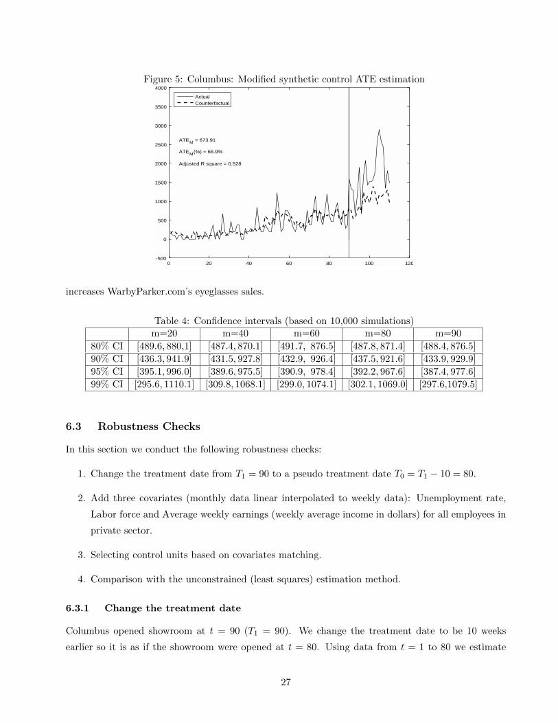
one should not apply the standard synthetic control method. However, we will show in Section 6 that

the modified estimation method can substantially reduce the estimation bias, giving a reliable ATE

estimation result for this empirical data.

2.3 The Modified Synthetic Control method

For many non-experimental data used in economics, marketing and other social science fields, the

treated unit and the control units may exhibit substantial heterogeneity and the treated unit’s outcome

7

and a weighted average (with weights sum to one) of the control units’ outcomes may not follow parallel

paths in the absent of treatment. In this section, we consider simple modifications as advocated by

Doudchenko and Imbens (2016). Specifically, we add an intercept and remove the coefficients sum to

one restriction in a standard synthetic control model, i.e., we still keep the non-negative constraints:

βj ≥ 0 for j = 2, ..., N , but drop the restriction∑Nj=2 βj = 1. When the sum of the estimated

weights (coefficients) is far from one, we suggest not to impose the add-to-one restriction. Therefore,

Doudchenko and Imbens’ modified synthetic control method is the same as (2.10) except that the

add-to-one restriction on the slope coefficients is removed, i.e., one solves the following (constrained)

minimization problem:

βT1,Msyn = arg minβ∈ΛMsyn

T1∑t=1

[y1t − x′tβ

]2, (2.13)

where xt = (1, y2t, ..., yNt)′, β is an N × 1 vector of parameters, and

ΛMsyn = β ∈ RN : βj ≥ 0 for j = 2, ..., N. (2.14)

Let X be the T1 ×N matrix with its ith row given by x′t = (1, y2t, ..., yNt), we show in Appendix

A that when X has full column rank (which requires that T1 ≥ N), the (modified) synthetic control

minimizers βT1,Syn and βT1,Msyn are uniquely defined.

With βT1,Msyn defined above, the counterfactual outcome is estimated by y01t = x′tβT1,Msyn for

t = T1 + 1, ..., T , and the ATE is estimated by

∆1,Msyn =1

T2

T∑t=T1+1

[y1t − y0

1t

]. (2.15)

3 Distribution Theory for the Synthetic Control ATE Estimator

3.1 Placebo Tests

Abadie and Gardeazabal (2003) and Abadie, Diamond and Hainmueller (2010) offer no formal inference

theory. Instead, they conduct placebo tests. Placebo tests evaluate the significance of estimates by

answering the question: under the null hypothesis of no treatment effect, how often would we obtain

an ATE estimate of a certain large magnitude purely by chance? Essentially, a placebo test involves

demonstrating that the effect does not exist when it is not expected to exist. In the case of the synthetic

control method, we first apply the synthetic control method to the treatment unit and calculate the

treatment effect. Then, we pretend that one of the control units (that did not receive treatment) is the

treatment unit and apply the synthetic control method. In this case, we expect the “treatment effect”

to be close to zero. This can be done iteratively for all the control units to obtain the “treatment

effect”. By plotting the treatment effects for the treatment unit and control units together, we should

see that the treatment effect for the true treatment unit has the greatest magnitude.

8

Abadie and Gardeazabal (2003) provide placebo test plots for California (treatment unit) and

38 control units. However, there were several control units whose treatment effects were of greater

magnitude than California. In order to address this concern, Abadie and Gardeazabal (2003) argue

that for certain control units, synthetic control method does not fit well enough in-sample (as measured

by the pre-intervention mean squared prediction error, MSPE). Therefore, they show three additional

placebo tests plots discarding states with MSPE twenty times higher, five times higher, and two times

higher than California, respectively. As expected, the placebo test plots look progressively better.

However, in practice, it is difficult to decide what the MSPE cutoff should be. In addition, placebo

tests can only provide correct confidence intervals under quite stringent conditions (Hahn and Shi

2016). To date, the majority of papers that use synthetic control also use placebo tests.

We provide the formal inference theory and show that subsampling can be used to obtain confidence

bounds and conduct hypothesis tests. To develop the inference theory, we use the theory of projections

onto convex sets. In the next few sections, we first formally present the synthetic control method

and modified synthetic control method as an optimization problem over a convex set and derive the

asymptotic distributions in order to facilitate formal inference.

3.2 A projection of the unconstrained estimator

To study the distribution theory of the synthetic control ATE estimator, we will first show that one

can express the constrained estimator as a projection of the unconstrained (the ordinary least squares)

estimator onto a constrained set. Then we use the theory of projection onto convex sets to derive the

asymptotic distribution of the synthetic control ATE estimator.

Let βOLS denote the ordinary least squares estimator of β0 using data y1t, xtT1t=1. We show in

Appendix A that the constrained estimator βT1 = arg minβ∈Λ∑T1t=1(y1t − x′tβ)2 can be obtained as a

projection of βOLS onto the convex set Λ, where Λ = ΛSyn or Λ = ΛMsyn.

We first define some projections. For θ ∈ RN , we define two versions of projection of θ onto a

convex set Λ as follows:

ΠΛ,T1θ = arg minλ∈Λ

(θ − λ)′(X ′X/T1)(θ − λ), (3.1)

ΠΛθ = arg minλ∈Λ

(θ − λ)′E(xtx′t)(θ − λ). (3.2)

Here we use the notation ΠΛ to denote a projection onto the set Λ. Note that the first projection

ΠΛ,T1 is with respect to a random norm ‖a‖X =√a′(X ′X/T1)a, while the second projection ΠΛ is

with respect to a non-random norm ‖a‖E =√a′E(xtx′t)a, i.e., ΠΛ,T1θ = arg minλ∈Λ ||λ − θ||2X and

ΠΛθ = arg minλ∈Λ ||λ−θ||2E . The first projection will be used to connect βT1 and βOLS , and the second

projection relates the limiting distributions of√T1(βT1 − β0) and

√T1(βOLS − β0).

9

With the above definition of the projection operator ΠΛ,T1 , we show in Appendix A that

βT1 = arg minβ∈Λ

(βOLS − β)′(X ′X/T1)(βOLS − β)

= arg minβ∈Λ||β − βOLS ||2X

= ΠΛ,T1 βOLS . (3.3)

Equation (3.3) says that the constrained estimator is a projection of the unconstrained estimator

onto the constrained set Λ.

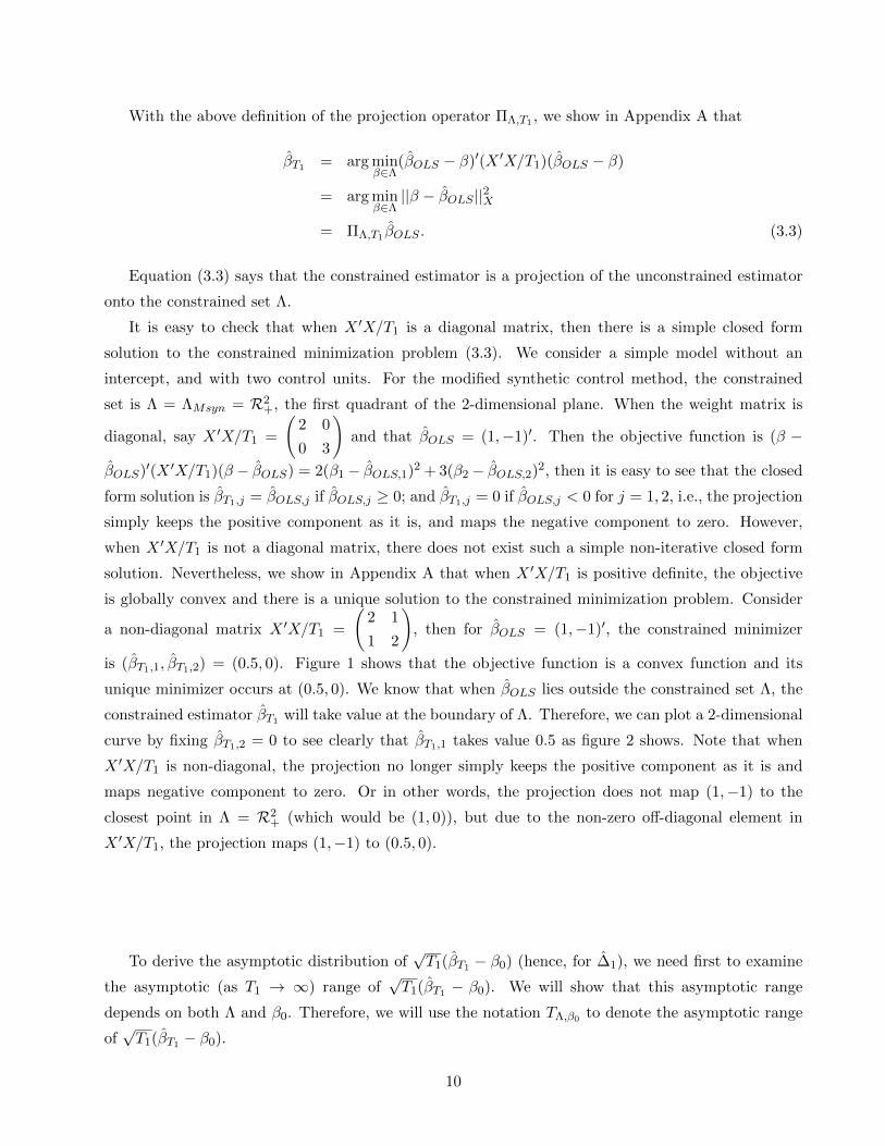
It is easy to check that when X ′X/T1 is a diagonal matrix, then there is a simple closed form

solution to the constrained minimization problem (3.3). We consider a simple model without an

intercept, and with two control units. For the modified synthetic control method, the constrained

set is Λ = ΛMsyn = R2+, the first quadrant of the 2-dimensional plane. When the weight matrix is

diagonal, say X ′X/T1 =

(2 0

0 3

)and that βOLS = (1,−1)′. Then the objective function is (β −

βOLS)′(X ′X/T1)(β − βOLS) = 2(β1 − βOLS,1)2 + 3(β2 − βOLS,2)2, then it is easy to see that the closed

form solution is βT1,j = βOLS,j if βOLS,j ≥ 0; and βT1,j = 0 if βOLS,j < 0 for j = 1, 2, i.e., the projection

simply keeps the positive component as it is, and maps the negative component to zero. However,

when X ′X/T1 is not a diagonal matrix, there does not exist such a simple non-iterative closed form

solution. Nevertheless, we show in Appendix A that when X ′X/T1 is positive definite, the objective

is globally convex and there is a unique solution to the constrained minimization problem. Consider

a non-diagonal matrix X ′X/T1 =

(2 1

1 2

), then for βOLS = (1,−1)′, the constrained minimizer

is (βT1,1, βT1,2) = (0.5, 0). Figure 1 shows that the objective function is a convex function and its

unique minimizer occurs at (0.5, 0). We know that when βOLS lies outside the constrained set Λ, the

constrained estimator βT1 will take value at the boundary of Λ. Therefore, we can plot a 2-dimensional

curve by fixing βT1,2 = 0 to see clearly that βT1,1 takes value 0.5 as figure 2 shows. Note that when

X ′X/T1 is non-diagonal, the projection no longer simply keeps the positive component as it is and

maps negative component to zero. Or in other words, the projection does not map (1,−1) to the

closest point in Λ = R2+ (which would be (1, 0)), but due to the non-zero off-diagonal element in

X ′X/T1, the projection maps (1,−1) to (0.5, 0).

To derive the asymptotic distribution of√T1(βT1 − β0) (hence, for ∆1), we need first to examine

the asymptotic (as T1 → ∞) range of√T1(βT1 − β0). We will show that this asymptotic range

depends on both Λ and β0. Therefore, we will use the notation TΛ,β0 to denote the asymptotic range

of√T1(βT1 − β0).

10

Figure 1: The constrained LS objective function

Figure 2: The objective function with b2 = 0

We note that even both βT1 and β0 take values at the constrained set Λ,√T1(βT1 − β0) does not

necessarily take values in Λ, the range of√T1(βT1−β0) depends on Λ as well as how many components

of the β0 vector taking value 0, i.e., it depends on how many non-negativity constraints are binding.

We illustrate this point via a simple example.

3.3 Examples of TΛ,β0, the asymptotic range of√T1(βT1 − β0)

3.3.1 Examples of TΛSyn,β0

We consider a simple case to illustrate the asymptotic range TΛSyn,β0 for the standard synthetic control

problem. For expositional simplicity, we consider a simple model of two control units and without an

intercept: y1t = x′tβ0 + u1t = x1tβ0,1 + x2tβ0,2 + u1t with β0 = (β0,1, β0,2)′ ∈ R2+ and β0,1 + β0,2 = 1.

The constrained set can be written as ΛSyn = β0 ∈ R2+, β0,1 ∈ [0, 1] and β0,2 = 1− β0,1.

To characterize TΛSyn,β0 for β0 ∈ ΛSyn, we consider the following three inclusive cases: (i) β0,1 = 0

and β0,2 = 1; (ii) β0,1 = 1 and β0,2 = 0; (iii) β0 ∈ (0, 1) and β0,2 = 1 − β0,1. It is easy to check that

for case (i), we have βT1,1 − β0,1 = βT1,1 ∈ [0, 1]. Hence,√T1(βT1,1 − β0,1) =

√T1βT1,1 ∈ [0,

√T1] →

[0,∞) = R+ as T1 → ∞. Similarly, we have√T1(βT1,2 − β0,2) =

√T1(βT1,1 − 1) ∈

√T1[−1, 0] =

[−√T1, 0] → (−∞, 0] = R− as T1 → ∞. Hence, the asymptotic range of

√T1(β − β0) for case (i) is

TΛSyn,β0,(i) = R+ × R−, which is the fourth quadrant. Similarly, for case (ii), one can easily show

11

that TΛSyn,β0,(ii) = R− ×R+, the second quadrant. Finally, for case (iii), since βj − β0,j can be either

positive or negative for j = 1, 2, hence,√T1(βj−β0,j) covers the whole real line as T1 →∞. Therefore,

we have TΛSyn,β0,(iii) = R2, the whole plane.

3.3.2 Examples of TΛMsyn,β0

We consider the same model as discussed in section 3.3.1 except that we now consider the modified

synthetic control method: y1t = x′tβ0 + u1t = x1tβ0,1 + x2tβ0,2 + u1t with β0 = (β0,1, β0,2)′ ∈ R2+. To

characterize TΛMsyn,β0 for β0 ∈ ΛMsyn = R2+, we consider four cases: (i) β0 = (0, 0)′; (ii) β0 = (0, β0,2)

with β0,2 > 0; (iii) β0 = (β0,1, 0) with β0,1 > 0; and (iv) β0 = (β0,1, β0,2) with β0,j > 0 for j = 1, 2. For

case (i) we have√T1(βT1,j − β0,j) =

√T1βT1,j ∈ [0,+∞) for j = 1, 2. Hence, TΛMsyn,β0,(i) = R+×R+,

which is the first quadrant. For case (ii), it is easy to see that√T1(βT1,1−β0,1) =

√T1βT1,1 ∈ [0,+∞),

and√T1(βT1,2 − β0,2) ∈

√T1[−β0,2,∞) → (−∞,+∞) = R as T1 → ∞. Hence, TΛMsyn,β0,(ii) =

R+ ×R, which is the union of the first and the fourth quadrants. Similarly, it is easy to check that

TΛMsyn,β0,(iii) = R×R+, the union of the first and the second quadrants. Finally, for case (iv), because

βT1,j − β0,j can be either positive or negative for j = 1, 2,√T1(βT1,j − β0,j)→ R as T1 →∞. Hence,

TΛMsyn,β0,(iv) = R×R, the whole plane.

Remark 3.1 Through the above examples one can see that TΛ,β0 gives the asymptotic range of√T1(βT1−

β0). Hence, it is quite intuitive to expect that the limiting distribution of√T1(βT1 − β0) can be repre-

sented as a projection of the limiting distribution of√T1(βOLS − β0) onto TΛ,β0.

We show in the next subsection that the intuition stated in remark 3.1 is indeed correct. We

present the result in the next subsection.

3.4 The asymptotic theory: the stationary data case

We term the set TΛ,β0 as the asymptotic range of√T1(βT1 − β0) based on intuitive argument. In the

projection theory, the set TΛ,β0 is termed as the tangent cone of Λ at β0. We give a formal definition

of a tangent cone as well as some explanation to the term ‘tangent’ in appendix B.

Theorem 3.2 Let Z1 denote the limiting distribution of√T1(βOLS−β0), then under the assumptions

1 to 4 presented in Appendix A, we have

√T1(βT1 − β0)

d→ ΠTΛ,β0Z1. (3.4)

Note that Theorem 3.2 states that the limiting distribution of the constrained estimator can be

represented as a projection of the unconstrained (least squares) estimator onto the tangent cone TΛ,β0 .

With the help of Theorem 3.2, we derive the asymptotic distribution of√T2(∆1 −∆1) as follows.

12

Theorem 3.3 Under the same conditions as in Theorem 3.2, we have

√T2(∆1 −∆1)

d→ −ηE(x′t)ΠTΛ,β0Z1 + Z2, (3.5)

where ∆1 = ∆1,Syn or ∆1,Msyn, ∆1 = E(∆1t), η = limT1,T2→∞√T2/T1, Z1 is defined in Theorem 3.2,

Z2 is independent with Z1 and distributed as N(0,Σ2), Σ2 = limT2→∞ T−12

∑Tt=T1+1

∑Ts=T1+1E(v1tv1s),

v1t = ∆1t − E(∆1t) + u1t, u1t has zero mean and is defined in (2.9).

The proof of Theorem 3.3 is given in Appendix B.

Although one can use projection theory to characterize the asymptotic distribution of√T1(∆1 −

∆1), the inference is not straightforward as one has to know β0 in order to calculate the tangent

cone TΛ,β0 . Fortunately, we will show in section 4 that a simple sub-sampling method can be used

to conduct valid inference. In particular, one does not need to know β0 when using the sub-sampling

method for inferences.

3.5 The Trend-Stationary data case

Up to now we only consider the stationary data case. However, many datasets, especially for panel

data with a long time dimension, exhibit some trending behaviors. For example, sales of a new product

tends to go up as more people get to know the product. In this subsection we extend the stationary

data result to the trend-stationary data case.

3.5.1 ATE estimation with Trend Stationary Data

From the previous analysis, we know that the synthetic control estimator is a projection of the

unconstrained least squares estimator onto the constrained set Λ; and the asymptotic theory of√T1(βSyn − β0) is the projection of the asymptotic distribution of

√T1(βOLS − β0) onto the tan-

gent cone TλSyn,β0 . Therefore, we will first study the asymptotic distribution of the unconstrained

least squares estimator using the pre-treatment data.

The trend-stationary data generating process can also be motivated using a factor model frame-

work. Let y0it, for i = 1, ..., N and t = 1, ..., T , be generated by some common factors with one of

the factor being a time trend and the remaining factors being weak dependent stationary variables.

Following Hsiao, Ching and Wan (2012) we assume that y0t = (y0

1t, y02t, ..., y

0Nt)′ is generated via a

factor model

y0t = δ0 +Bft + εt, (3.6)

where δ0 = (δ01, ..., δ0N )′ is an N × 1 vector of intercepts, B is an N × K factor loading matrix,

ft = (f1t, ..., fKt)′ is a K × 1 vector of common factors, εt = (ε1t, ..., εNt)

′ is an N × 1 vector of

idiosyncratic errors. We assume that f1t = t and all other factors are stationary variables. Also, εt is a

13

zero mean, weakly dependent process with finite fourth moment. Hence, y0t follows a trend-stationary

process.

Hsiao, Ching and Wan (2012), and Li and Bell (2017) show that, under the condition that

rank(B) = K, one can replace the unobservable factor ft by xt = (1, y2t, ..., yNt)′ to estimate the

counterfactual outcome y01t. Specifically, one can estimate the following regression model

y1t = x′tδ + u1t, (t = 1, ..., T1), (3.7)

where xt = (1, y2t, ..., yNt)′ and δ = (δ1, ..., δN )′.

To facility the asymptotic analysis, below we consider the time trend component explicitly. We

write yjt = c0,j + c1,jt + y∗jt, where y∗jt is a weakly dependent stationary process (de-trended from

yjt) for j = 2, ..., N . Let yt = (y2t, ..., yNt)′ and δ = (δ2, ..., δN )′. Then in vector notation, we have

yt = c0 + c1t+ y∗t , c0 = (c0,2, ..., c0,N )′, c1 = (c1,2, ..., c1,N )′ and y∗t = (y∗2t, ..., y∗Nt)′. Then we can write

y′tδ = (c0 + c1t+ y∗t )′δ. Hence, we can re-write (3.7) as

y1t = δ1 + y′tδ + u1t

= α0t+ β1 + δ′y∗t + u1t

= α0t+ z′tβ0 + u1t t = 1, ..., T1, (3.8)

where α0 = c′1δ, β1 = δ1 + c′0δ, β0 = (β1, δ′)′ and zt = (1, y∗

′)′ ≡ (1, y∗2t, ..., y

∗Nt)′.

Let αT1 and βT1 be the constrained least squares estimators of α0 and β0 subject to βj ≥ 0

for j = 2, ..., N and∑Nj=2 βj = 1 for the synthetic control estimator; or dropping the sum to one

restriction for the modified synthetic control estimator using the pre-treatment data. We estimate y01t

by y01t = αT1t+ z′tβT1 and estimate the ATE is estimated by

∆1 =1

T2

T∑t=T1+1

∆1t, (3.9)

where ∆1t = y1t − y01t.

3.5.2 Asymptotic Theory with Trend Stationary Data

To derive the asymptotic distribution of√T2(∆1 − ∆1), we need first present the theory for the

unconstrained least squares estimator of γ0 = (α0, β′0)′. Let γOLS denote the ordinary least squares

estimator of γ0. Define MT1 =√T1diag(T1, 1, ..., 1), which is an (N + 1) × (N + 1) diagonal matrix

with its first diagonal element equals to T3/21 and all other diagonal elements equal to

√T1. Then, it

is well established that (e.g., Hamilton (1994))

MT1(γOLS − γ0)d→ N(0,Ω), (3.10)

14

where Ω is a (N + 1) × (N + 1) positive definite matrix whose explicit definition can be found in

Hamilton (1994, Chapter 16).

We still use Λ to denote constrained sets for γT1 for trend-stationary data case. Now γ is an

(N + 1) × 1 vector whose first component is the time trend coefficient, the second component is the

intercept. Hence, the constrained sets for the standard and the modified synthetic control models are

ΛSyn = γ ∈ RN+1 : γj ≥ 0 for j = 3, ..., N + 1,∑N+1j=3 γj = 1; (3.11)

ΛMsyn = γ ∈ RN+1 : γj ≥ 0 for j = 3, ..., N + 1. (3.12)

Define the synthetic control estimator

γT1 = arg minγ∈Λ

T1∑t=1

(y1t − w′tγ)2, (3.13)

where wt = (t, z′t)′, Λ = ΛSyn or ΛMsyn. Then similar to Theorem 3.2, we have

Theorem 3.4 Let Z3 denote the limiting distribution of√T1(γOLS − γ0) as described in (3.10), then

under the assumptions D1 to D3 presented in the supplementary Appendix D, we have

√T1(γT1 − γ0)

d→ ΠTΛ,γ0Z3, (3.14)

where TΛ,γ0 is the tangent cone of Λ evaluated at γ0, Z3 is the weak limit of MT1(γOLS−γ0) as described

in (3.10).

With Theorem 3.4 we can derive the asymptotic distribution of√T2(∆1 −∆1).

Theorem 3.5 Under the same conditions as in Theorem 3.2, we have

√T2(∆1 −∆1)

d→ −c′ΠTΛ,γ0Z3 + Z2, (3.15)

where ∆1 is defined in (3.9), ∆1 = E(∆1t), c = (√η(2 + η),

√ηE(z′t))

′, η = limT1,T2→∞√T2/T1, Z3

is the limiting distribution of MT1(γOLS − γ0) as defined in (3.10), Z2 is independent with Z3, and it

is normally distributed with zero mean and variance Σ2 = limT2→∞ T−12

∑Tt=T1+1

∑Ts=T1+1E(v1tv1s),

vit = ∆1t −∆1 + u1t.

The proof of Theorem 3.5 is similar to the proof of Theorem 3.3 and is thus omitted.

4 Inference Theory

In this section we discuss inference methods for the ATE estimator ∆1. For expositional simplicity,

we will only discuss inferences for the stationary data case. For trend-stationary data, one can first

15

de-trend the data, then using the inference method discussed in this section for the de-trended data.

In section 4.1 we consider the case that both T1 and T2 are large, while in section 4.2 we deal with

the small T2 case.

4.1 Sub-sampling method

As discussed in the above section, the inference theory for the synthetic control estimator is compli-

cated. The asymptotic distribution of βT1 depends on whether β0,j = 0 or β0,j > 0 for j = 2, ..., N .

When β0,j > 0 for all j = 2, ..., N , asymptotically, the constraints are non-binding and the asymptotic

theory of the constrained estimator is the same as that of the unconstrained ordinary least squares

estimator. However, when the constraints are binding for some j ∈ 2, ..., N, the asymptotic distri-

bution of the constrained estimator is much more complex (e.g., (3.4)). The asymptotic distribution

of the synthetic control coefficient estimators depends on whether the true parameters take value at

the boundary or not. In practice we do not know which constraints are binding and which are not,

making it more difficult to use the asymptotic theory for inference. Moreover, it is known that when

parameters fall to the boundary of the parameter space, the standard bootstrap method does not work

(e.g., Andrews (2000), Fang and Santos (2015)). We resolve this difficulty by proposing an easy-to-

implement sub-sampling method. The proposed sub-sampling method works whether constraints are

binding, partially binding or non-binding. That is, the sub-sampling method is adaptive in the sense

that we do not need to know whether constraints are binding and if they are binding, we do not need

to know bindings are on which coefficients.1

We use m to denote the sub-sample size. We will show that ∆1 can be decomposed into two terms,

one term is related to the constrained estimator βT1 , the second term is unrelated to βT1 but depends

on T2, it can be shown that a brute-force application of the sub-sampling method will not work in

general. The correct method is to first isolate the term√T1(βT1 − β0) from other terms, and apply

the sub-sampling method only to√T1(βT1 − β0).

For the whole sample period, the outcome y1t is generated by

y1t = x′tβ0 + dt∆1t + u1t, t = 1, ..., T1, ..., T, (4.1)

where dt is the post-treatment time period dummy so that dt = 0 if t ≤ T1 and dt = 1 if t ≥ T1 + 1.

Substituting (4.1) into (3.5) we obtain

Adef=

√T2(∆1 −∆1)

1Hong and Li (2017) show that numerical differentiation bootstrap method can consistently estimate the limitingdistribution in many cases where the conventional bootstrap is known to fail. One can also use Hong and Li’s (2017)method to conduct inference for the synthetic control estimator. In this paper we focus on the simple sub-samplingmethod.

16

=1√T2

T∑t=T1+1

(y1t − y01t −∆1)

=1√T2

T∑t=T1+1

(x′tβ0 + ∆1t + u1t − x′tβT1 −∆1)

= −√T2

T1

1

T2

T∑t=T1+1

x′t

√T1(βT1 − β0) +1√T2

T∑t=T1+1

(∆1t −∆1 + u1t)

≡ −√T2

T1

1

T2

T∑t=T1+1

x′t

√T1(βT1 − β0) +1√T2

T∑t=T1+1

v1t, (4.2)

where v1t = ∆1t −∆1 + u1t.

Now we impose an additional assumption that u1t and v1t are both serially uncorrelated. This

assumption greatly simplifies the sub-sampling method that will be discussed below. This assumption

can be tested easily in practice. When this assumption is violated, more sophisticated method such

as block sub-sampling method can be used to deliver valid inferences.

Expression (4.2) suggests that we only need to apply the sub-sampling method to the term√T1(βT1 − β0) because only this term is related to the constrained estimator. We now describe

the sub-sampling steps. In Appendix B we show that, when v1t is serially uncorrelated, one can con-

sistently estimate Σ2 by Σ2 = 1T2

∑Tt=T1+1 v

21t, where v1t = ∆1t − ∆1. We generate v∗1t ∼ iid N(0, Σ2)

for t = T1 + 1, ..., T . Next, let m be the sub-sample size that satisfies the condition that m→∞ and

m/T1 → 0 as T1 →∞. For t = 1, ...,m, we randomly draw (y∗1t, x∗t ) from y1t, xtT1

t=1 without replace-

ment (sub-sampling). Then we use the sub-sample y∗1t, x∗t mt=1 to estimate β0 by the constrained least

squares method, i.e., β∗m = arg minβ∈Λ∑mt=1(y∗1t − x∗

′t β)2. The sub-sampling/bootstrap version of the

statistic A is given by

A∗ = −√T2

T1

1

T2

T∑t=T1+1

x′t

√m(β∗m − βT1) +1√T2

T∑t=T1+1

v∗1t. (4.3)

We repeat the above process for a large number of times, say, J times. Using A∗jJj=1, we can

obtain confidence intervals for A.

Let A∗(1) ≤ A∗(2) ≤ ... ≤ A

∗(J). Then the 1− α confidence interval for ∆1 is given by

[∆1 − T−1/22 A∗(1−α/2) , ∆1 − T−1/2

2 A∗(α/2)]. (4.4)

We show that the above method indeed gives consistent estimation of the confidence intervals for

∆1 in the next Theorem.

Theorem 4.1 Under the same conditions as in Theorem 3.3, also assuming that m→∞ and m/T1 →0 as T1 →∞, then for any α ∈ (0, 1), the (1−α) confidence interval of ∆1 can be consistently estimated

17

by [∆1 − T−1/22 A∗(1−α/2) , ∆1 − T−1/2

2 A∗(α/2)].

The sub-sampling method is a powerful tool for inference. It works under quite general conditions

even when the regular bootstrap method does not work as in the case of the synthetic control ATE

estimator. Politis, Romano and Wolf (1999)) provide proofs/arguments showing that ‘sub-sampling

method works’ under very weak regularity conditions.

Remark 4.2 Note that even we random draw (y∗t , x∗t ) from ys, xsT1

s=1 for t = 1, ...,m, we do not

require that ys, xsT1s=1 to be a serially uncorrelated process. In fact, they can have arbitrary serial

correlation, say yjtNj=1 is generated by some serially correlated common factors, we only need that

idiosyncratic error u1t in (2.9) is serially uncorrelated. This can be easily tested given data. In section

5 we generate yjt using a three factor model, where the three factors follow AR, ARMA and MA

processes, respectively. Simulations show that the above proposed sub-sampling method works well.

When u1t is serially correlated, we conjecture that one replace the random sub-sampling method by

block sub-sampling method. We leave the formal justification of using block sub-sampling method as a

future research topic.

Remark 4.3 In the literature of sub-sampling method, the choice of sub-sample size m is a key issue.

Bickel and Sakov (2008) propose a data-driven method to select m. In general, too small an m or too

large an m do not work well, when m falls into an appropriate interval, the performance should be

stable and acceptable. For our model, because β0,j > 0 for some j ∈ 2, ..., N, and that the statistic

√T2(∆1 −∆1) = −

√T2

T1

1

T2

T∑t=T1+1

x′t

√T1(βT1 − β0) +1√T2

T∑t=T1+1

v1t, (4.5)

also contains a term T−12

∑Tt=T1+1 v1t, where v1t = ∆1t−∆1 +u1t, which is not related to βT1. It turns

out that the sub-sampling method works well for a wider range of m. We will discuss more on this

issue at Section 5.3 and at the supplementary Appendix D.

4.2 Inference theory when T2 is small

The asymptotic theories presented in section 4.1 assume that both T1 and T2 are large. However,

in practice, many datasets have T2 much smaller than T1. When T2 is small, Ferman and Pinto

(2016a) propose using Andrews’ (2003) end-of-sample instability test to conduct inference for DID

and synthetic control ATE estimators. In this subsection we discuss using Andrews’s test to conduct

inferences for the ATE estimator based on the synthetic control method.

When T1 is large and T2 is small, the first term on the right-hand-side of (4.2) has an order

18

Op(√T2/T1) = Op(T

−1/21 ) becomes negligible, then we have

A =1√T2

T∑t=T1+1

(y1t − y01t −∆1) =

1√T2

T∑t=T1+1

v1t + op(1), (4.6)

where v1t = ∆1t −∆1 + u1t has zero mean and finite variance.

One can test the null hypothesis of a constant treatment effects H0: ∆1t = ∆1,0 for some pre-

specified value ∆1,0 for t = T1 + 1, ..., T , against, say, a one-sided positive treatment effects H1:

∆1 = E(∆1t) > ∆1,0 for t = T1 + 1, ..., T . Following Andrews (2003), we can use the following test

statistic

BT2 =1√T2

T∑t=T1+1

(y1t − y01t −∆1,0) =

1√T2

T∑t=T1+1

v1t,0 + op(1), (4.7)

where v1t,0 = ∆1t − ∆1,0 + u1t. Under H0 we have v1t,0 = u1t has zero mean, and it has a positive

mean under H1.

To conduct inference based on the test statistic BT2 , we compute the following quantity

BT2,jdef=

1√T2

T2+j−1∑t=j

u1t =1√T2

T2+j−1∑t=j

u1t +Op(T−1/21 ), for j = 1, ..., T1 + 1− T2, (4.8)

where for t = 1, ..., T1, u1t = y1t − y01t = x′t(β0 − βT1) + u1t = u1t + Op(T

−1/21 ) because βT1 − β0 =

Op(T−1/21 ). The empirical distribution of B2,jT1+1−T2

j=1 can be used to obtain critical values for the

test statistic BT2 under the null hypothesis H0: ∆1t = ∆1,0 for all t = T1 + 1, ..., T . If BT2 is at the

tail of this empirical distribution, we reject the null hypothesis and accept the alternative hypothesis.

Remark 4.4 We can only test a constant treatment effects for each post-treatment period using An-

drews’ test, i.e., we can only test ∆1,t = ∆1,0 for all t = T1 + 1, ..., T . We cannot test ∆1 = ∆1,0

because under this null hypothesis, we will have ∆1,t − ∆1 = ∆1t − ∆1,0 has a zero mean and a fi-

nite variance, we cannot use pre-treatment data to estimate the variance of ∆1t. Therefore, Andrews’

method become invalid when treatment effects varies with t.

Remark 4.5 Andrews’ test will have good estimated sizes for large T1. However, it is not a consistent

test because T2 is small. The power of the test depends on the strength of the treatment effects under

H1. The power of the test should increase with T2, but when T2 is large, an estimation error of order√T2/T1 may become non-negligible, rendering Andrews’ test invalid in our context, see section 5.3 for

a more detailed discussion on this issue.

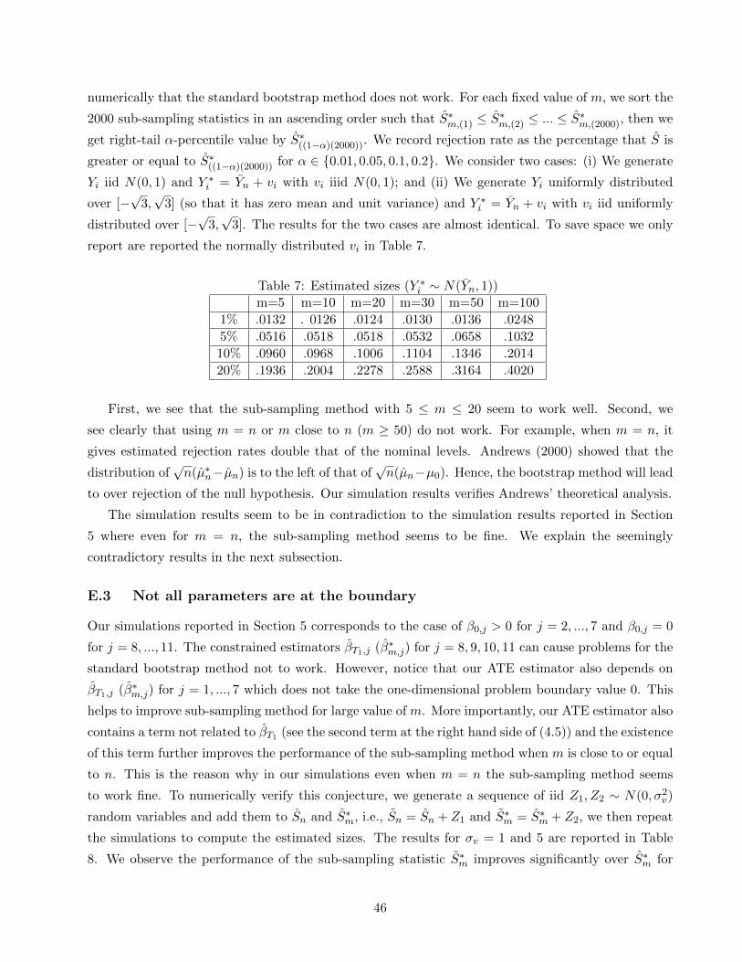
5 Monte Carlo simulations

In this section we first consider the case of large T1 and T2 and examine the performance of sub-

sampling method inferences through simulations, then we consider the case of large T1 and small T2

19

and examine the performance of Andrews’ (2003) end-of-sample instability test.

5.1 A three factor data generating process

We conduct simulation studies using the same data generating process as in Hsiao, Ching and Wan

(2012) and Du and Zhang (2015). We consider the same 3-factor model as follows.

f1t = 0.8f1t−1 + ε1t,

f2t = −0.6f1t−1 + ε2t + 0.8ε2t−1,

f3t = ε3t + 0.9ε3t−1 + 0.4ε3t−2,

where εit is iid N(0, 1). Let y0t denote the N × 1 vector of outcome variables without treatment. It is

generated via the factor model

y0t = a+Bft + ut, t = 1, ..., T (5.1)

where y0t = (y0

1t, y02t, ..., y

0Nt)′, a = (a1, a2, ..., aN )′ and ut = (u1t, u2t, ..., uNt)

′ are all N × 1 vectors,

B = (b1, b2, ..., bN )′ is the N × 3 loading matrix where bj is a 3 × 1 loading vector for unit j, ft is

the 3× 1 common factors: ft = (f1t, f2t, f3t)′. We choose (a1, a2, ..., aN ) = (1, 1, ..., 1), εjt iid N(0, σ2)

with σ2 = 0.5.

We use a set up similar to our Warby Parker empirical data by setting T1 = 90, T2 = 20, T =

T1 + T2 = 110 and N = 11 (with 10 control units). For factor loadings, we use b1 to denote the 3× 1

vector of loadings for the first unit (the treated unit); use b2 = (b2, ..., bs+1) denote 3×s loading matrix

for units j = 2, ..., s+ 1 (1 ≤ s ≤ N − 2); finally we use b3 = (bs+1, ..., bN ) denote the 3× (N − 1− s)loading matrix for the last N − s− 1 units. We fix s = 6 and consider the following two sets for factor

loadings:

DGP1 : b1 = 13×1; bj = 13×1 for j = 2, ..., 7; and bj = 03×1 for j = 8, ..., 11,

DGP2 : b1 = 2(13×1); bj = 13×1 for j = 2, ..., 7; and bj = 03×1 for j = 8, ..., 11,

where 13×1 and 03×1 denote 3× 1 vectors of ones and zeros, respectively.

Note that for both DGP1 and DGP2, 6 out of 10 control units have non-zero loadings and the

remaining 4 control units have zero loadings. Also note that for DGP1, all non-zero factor loadings

are set to be ones so that the treated and the control units (with non-zero loadings) are drawn from a

common distribution. While for DGP2, loadings for the treated unit all equal to 2, and the controls

units’ loadings (with non-zero loadings) are all equal to 1. Thus, the treated and control units are

drawn from two heterogeneous distributions.

20

We generate the following treatment effects ∆1t:

∆1t = α0

[ezt

1 + ezt+ 1

], t = T1 + 1, ..., T, (5.2)

where zt = 0.5zt−1 + ηt and ηt is iid N(0, 0.52).

Note that for post-treatment period, y1t = y11t = y0

1t + ∆1t, where y01t are generated as described

earlier and ∆1t is generated by (5.2). There is a zero, or a positive treatment effects corresponding to

α0 = 0 and α0 > 0, respectively.

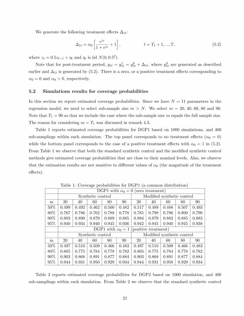
5.2 Simulations results for coverage probabilities

In this section we report estimated coverage probabilities. Since we have N = 11 parameters in the

regression model, we need to select sub-sample size m > N . We select m = 20, 40, 60, 80 and 90.

Note that T1 = 90 so that we include the case where the sub-sample size m equals the full sample size.

The reason for considering m = T1 was discussed in remark 4.3.

Table 1 reports estimated coverage probabilities for DGP1 based on 1000 simulations, and 400

sub-samplings within each simulation. The top panel corresponds to no treatment effects (α0 = 0)

while the bottom panel corresponds to the case of a positive treatment effects with α0 = 1 in (5.2).

From Table 1 we observe that both the standard synthetic control and the modified synthetic control

methods give estimated coverage probabilities that are close to their nominal levels. Also, we observe

that the estimation results are not sensitive to different values of α0 (the magnitude of the treatment

effects).

Table 1: Coverage probabilities for DGP1 (a common distribution)DGP1 with α0 = 0 (zero treatment)

Synthetic control Modified synthetic control

m 20 40 60 80 90 20 40 60 80 90

50% 0.499 0.492 0.462 0.500 0.482 0.517 0.489 0.488 0.507 0.49380% 0.767 0.786 0.762 0.788 0.778 0.785 0.798 0.786 0.800 0.79090% 0.883 0.890 0.879 0.889 0.885 0.894 0.879 0.882 0.885 0.88395% 0.940 0.934 0.940 0.945 0.936 0.942 0.945 0.940 0.945 0.938

DGP1 with α0 = 1 (positive treatment)


m 20 40 60 80 90 20 40 60 80 90

50% 0.497 0.510 0.509 0.466 0.483 0.497 0.510 0.509 0.466 0.48380% 0.805 0.775 0.784 0.778 0.782 0.805 0.775 0.784 0.778 0.78290% 0.903 0.868 0.891 0.877 0.884 0.903 0.868 0.891 0.877 0.88495% 0.944 0.931 0.950 0.929 0.934 0.944 0.931 0.950 0.929 0.934

Table 2 reports estimated coverage probabilities for DGP2 based on 1000 simulation, and 400

sub-samplings within each simulation. From Table 2 we observe that the standard synthetic control

21

method give biased estimation results. The estimated coverage probabilities are much smaller than

the corresponding nominal values. The reason for this biased estimation result is that for DGP2,

the treated and the control units are drawn from different distributions because they have different

factor loadings. In contrast to the standard synthetic control approach, the modified synthetic control

method give good estimated coverage probabilities. This verifies that the modified synthetic control

method is robust to data drawn from heterogeneous distributions. Like the case of DGP1, the results

are not sensitive to different values of α0.

Table 2: Coverage probabilities for DGP2 (a heterogenous distribution)DGP2 with α0 = 0 (zero treatment)


m 20 40 60 80 90 20 40 60 80 90

50% 0.294 0.308 0.314 0.292 0.306 0.474 0.458 0.492 0.474 0.47080% 0.526 0.534 0.522 0.510 0.540 0.776 0.756 0.770 0.742 0.73890% 0.658 0.630 0.638 0.632 0.666 0.884 0.854 0.876 0.844 0.86695% 0.752 0.710 0.720 0.720 0.754 0.936 0.924 0.930 0.908 0.926

DGP2 with α0 = 1 (positive treatment)


m 20 40 60 80 90 20 40 60 80 90

50% 0.306 0.278 0.276 0.278 0.286 0.508 0.486 0.468 0.478 0.48280% 0.522 0.478 0.510 0.472 0.496 0.802 0.764 0.796 0.796 0.77090% 0.634 0.614 0.620 0.580 0.594 0.888 0.890 0.894 0.894 0.88495% 0.710 0.716 0.710 0.678 0.668 0.948 0.944 0.940 0.950 0.944

5.3 Inferences when T2 is small

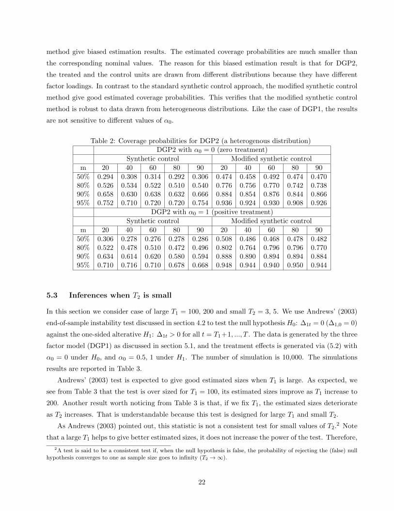
In this section we consider case of large T1 = 100, 200 and small T2 = 3, 5. We use Andrews’ (2003)

end-of-sample instability test discussed in section 4.2 to test the null hypothesis H0: ∆1t = 0 (∆1,0 = 0)

against the one-sided alterative H1: ∆1t > 0 for all t = T1 +1, ..., T . The data is generated by the three

factor model (DGP1) as discussed in section 5.1, and the treatment effects is generated via (5.2) with

α0 = 0 under H0, and α0 = 0.5, 1 under H1. The number of simulation is 10,000. The simulations

results are reported in Table 3.

Andrews’ (2003) test is expected to give good estimated sizes when T1 is large. As expected, we

see from Table 3 that the test is over sized for T1 = 100, its estimated sizes improve as T1 increase to

200. Another result worth noticing from Table 3 is that, if we fix T1, the estimated sizes deteriorate

as T2 increases. That is understandable because this test is designed for large T1 and small T2.

As Andrews (2003) pointed out, this statistic is not a consistent test for small values of T2.2 Note

that a large T1 helps to give better estimated sizes, it does not increase the power of the test. Therefore,

2A test is said to be a consistent test if, when the null hypothesis is false, the probability of rejecting the (false) nullhypothesis converges to one as sample size goes to infinity (T2 →∞).

22

Table 3: Coverage probabilities for DGP1 (Andrews’ instability test)H0: α0 = 0

T2 = 3 T2 = 5

T1 5% 10% 20% 5% 10% 20%

100 0.0849 0.1362 0.2366 0.0935 0.1497 0.2440

200 0.0652 0.1161 0.2191 0.0711 0.1250 0.2273

H1: α0 = 0.5

T2 = 3 T2 = 5

T1 5% 10% 20% 5% 10% 20%

100 0.2892 0.4076 0.6656 0.3492 0.4753 0.6985

H1: α0 = 1

T2 = 3 T2 = 5

T1 5% 10% 20% 5% 10% 20%

100 0.5416 0.6573 0.7937 0.6994 0.7939 0.8853

we only consider T1 = 100 for power calculation because for T1 = 200 or even larger T1, the powers

of the test are similar. When T1 is large, the power of the test increases with T2 and also depends

on the magnitude of∑Tt=T1+1(∆1t −∆1,0) under H1. From Table 3 we see that the estimated power

increases with T2 as well as with α0 (the magnitude of ∆1t). However, a large T2 adversely affects the

estimated sizes of Andrews’ test.

We also conducted simulations of Andrews’ test under DGP1 using T1 = 90 and T2 = 20 (same

T1 and T2 as in our empirical data). Based on 10,000 simulations with α0 = 0, the estimated sizes

are 0.1660, 0.1964 and 0.2699 for nominal levels 5%, 10%, and 20%, respectively. We see that for

T2 = 20, T1 = 90 is not large enough for the test to have good estimated sizes, because an error term

of order√T2/T1 is not negligible which causes Andrews’ test invalid in our context. Therefore, the

end-of-sample stability testing and the sub-sampling testing procedures are complement to each other.

The former can be used when T2 is small, while the later is preferred when T2 is not small.

Remark 5.1 Here for our synthetic control ATE estimator with panel data, large T2 invalidates An-

drews’ test due an error term of order√T2/T1 becoming non-negligible. This differs from the time

series model considered by Andrews (2003), where when T2 is also large, testing a possible structure

break at T1 becomes a simple and standard problem.

6 An Empirical Application

In this section we present an empirical application to illustrate the usefulness of the modified synthetic

control method in practice. In the application, we calculate the ATE based on the modified synthetic

control method and the confidence intervals using the sub-sampling method.

23

6.1 Warby Parker and ATE estimation

We have data from WarbyParker.com whose mission is to provide high quality products at lower

prices ($95 instead of $300+range). In February 2010, WarbyParker.com opened its first physical

showroom at the New York City headquarter. Later, they opened more showrooms in several cities

hoping that opening physical showrooms can significantly promote sales. They opened a showroom

in Columbus, Ohio on October 11, 2011. In this section, we want to evaluate how the showroom

opening in Columbus affects Columbus’ average weekly sales (the average treatment effect) in the

post-treatment period. As discussed in section 2 on estimating treatment effects using panel data,

we estimate the counterfactual sales for Columbus by letting the sales of Columbus be the dependent

variable, and the control cities’ sales (sales in cities without showrooms) be the explanatory variables.

Hence, we run a constrained regression, i.e., we regress weekly sales of Columbus on sales of control

cities to obtain the estimated coefficients under the restriction that the coefficients are non-negative.

Then, using these estimated coefficients, together with the post-treatment period sales for the control

group cities, we compute the counterfactual of what sales would be for Columbus in the absence of the

showroom opening. The 10 largest cities (by population) that do not have showrooms were selected

as the control group cities. These cities are: Atlanta, Chicago, Dallas, Denver, Houston, Minneapolis,

Portland, San Diego, Seattle and Washington.

First, we would like to show that “parallel lines” assumption is violated for this data. Hence, DID

and the standard synthetic control methods should not be used to estimate ATE for this data.

Figure 3: Columbus: DID fitted curve

0 20 40 60 80 100 120

-1000

-500

0

500

1000

1500

2000

2500

3000

3500

ActualCounterfactual

In figure 3, the solid line denotes Columbus’ weekly sales (in dollars) while the dashed line is fitted

curve using the DID method which is computed using (2.8). The vertical line denotes the time of

showroom opening (occurred at T1 = 90th week). We see that the DID fitted curve and the real data

have different upward trends. This is a case that DID method should not be used to estimate ATE.

However, if one mis-applies the DID method to estimate ATE, one would obtain a severely biased

24

estimation result. The DID fitted curve underestimates Columbus’ sales for the first half sample (from

t = 1 to about t = T1/2) and overestimates the sales for the second half sample (from t = T1/2 + 1 to

t = T1). As a result, DID would overestimate the out-of-sample counterfactual outcome (for t ≥ T1 +1

with T2 = 20). Consequently, DID would underestimate the average treatment effects.

The problem with the DID method when applied to Columbus’ data is that the average of the

10 control cities’ sale sand Columbus’ sales exhibit different upward trends during the pre-treatment

period data (in the absence of treatment). Therefore, the simple average of these control cities’

sales predicted Columbus’ counterfactual sales poorly. The validity of the DID method relies on the

assumption that the Columbus’ sales and the average of control cities’ sales follow parallel paths in

the absence of treatment (for pre-treatment period). This assumption is violated for the data we have.

Next, we examine the standard synthetic control method. Figure 4 plots Columbus’ actual sales

(solid line) and the in-sample-fit and out-of-sample counterfactual forecast (dotted line) curve com-

puted using (2.12). From figure 4, we see that the synthetic control method’s in-sample-fit is also

poor as it underestimates the actual sales for the first half of the in-sample data and overestimates

the actual sales for the second half of the in-sample data. In this case, one should not use the stan-

dard synthetic control method to estimate ATE. Nevertheless, we can also see that if one mis-applies

the synthetic control method to this data set, one would overestimate the counterfactual outcome

which would result in an underestimation of ATE. The reason for this is that without the restriction

that coefficients-add-to-one, the sum of the slope coefficients is 0.234. The standard synthetic control

method imposes the slope coefficients to add to one, which inflates the slope of fitted curve to be larger

than the slope of the actual data. The estimated intercept moves the fitted curve down parallel in an

attempt to make the fitted curve and the actual data have the same sample mean (for pre-treatment

period data). This leads to the fitted curve that is below the actual data for the first half of the sample

data and above the actual data for the second half of the sample data. Hence, it leads to a significant

overestimation of the out-of-sample counterfactual sales, which in turn leads to a severely downward

biased estimated ATE.

The above analysis suggests that restricting the slope coefficients to add to one is the reason for

a large estimation bias of the standard synthetic control method. Therefore, we relax the weights

add-to-one condition, i.e., we only keep the non-negativity of the weights but drop the add-to-one

restriction. Applying this ‘modified synthetic control method’ to Columbus’ data, we obtain that the

estimated weights add up to 0.234 which is substantially less than one. The estimation results are

plotted in Figure 5. The results in figure 5 show a much improved in-sample-fit. Unlike Figures 3 and

4, the fitted curve in figure 5 does not appear to have any systematic estimation bias (for 1 ≤ t ≤ T1).

Our estimation result shows that opening a showroom in Columbus on November 10, 2011 leads to

an average 67% increase in weekly sales. In the next subsection we show that the estimated positive

ATE is statistically highly significant.

25

Figure 4: Columbus: The synthetic control fitted curve

0 20 40 60 80 100 120-500

0

500

1000

1500

2000

2500

3000

3500

4000


6.2 Confidence intervals for the ATE

In this section we use the sub-sampling method discussed in Section 4 to estimate confidence intervals

(CI) for the ATE (∆1). Since our proposed sub-sampling method requires that the idiosyncratic error

u1t defined in (2.9) be serially uncorrelated, we will first test whether this assumption holds true for

the data we have. Let u1t = y1t − x′tβT1 , then a simple statistic for testing zero serial correlation is√T1ρ =

√T1∑T1t=2 u1tu1,t−1/

∑T1t=2 u

21t. Under the null hypothesis of zero serial correlation,

√T1ρ has

a standard normal distribution (for large T1). For Columbus sales’ data, we obtain√T1ρ = 0.7281,

which gives a p-value of 0.467. Therefore, the empirical data supports the null hypothesis that there

is no zero serial correlation in the idiosyncratic error u1t, justifying the use of the simple sub-sampling

method discussed in section 4.

To conduct the sub-sampling inference, we choose sub-sample sizes m = 20, 40, 60, 80, 90. For each

value of m, we conduct 10,000 sub-sampling simulations ∆1 − T−1/22 A∗j

10,000j=1 . We then sort these

10,000 statistics to obtain α/2 percentile and (1−α/2) percentile for α = 0.2, 0.1, 0.05 and 0.01. The

results are given in Table 4.

First, we observe that the estimated confidence intervals are quite similar for different sub-sample

sizes, including the case of m = T1 (recall that T1 = 90). The empirical data example further verifies

that, due to the reason discussed in remark 4.3, the sub-sampling method works well for a wide range

of m values. Next, we notice that the lower bound of these intervals are all positive and far above

zero for all m values. This implies that the estimated ATE value of 674.5 is positive and significantly

different from zero for all conventional significant levels. In fact, if we conduct a 1% level test, we will

reject ∆1 = 295 and in favor of ∆1 > 295 because 99% CIs are at the right of 295 for all m values

considered. Similarly, if we conduct a 10% level test, we will reject ∆1 = 430 and in favor of ∆1 > 430

because all 90% CIs are at the right of 430. Thus, opening a showroom at Columbus significantly

26

Figure 5: Columbus: Modified synthetic control ATE estimation

0 20 40 60 80 100 120-500

0

500

1000

1500

2000

2500

3000

3500

4000

ATEM = 673.91

ATEM(%) = 66.9%

Adjusted R square = 0.528


increases WarbyParker.com’s eyeglasses sales.

Table 4: Confidence intervals (based on 10,000 simulations)m=20 m=40 m=60 m=80 m=90

80% CI [489.6, 880,1] [487.4, 870.1] [491.7, 876.5] [487.8, 871.4] [488.4, 876.5]

90% CI [436.3, 941.9] [431.5, 927.8] [432.9, 926.4] [437.5, 921.6] [433.9, 929.9]

95% CI [395.1, 996.0] [389.6, 975.5] [390.9, 978.4] [392.2, 967.6] [387.4, 977.6]

99% CI [295.6, 1110.1] [309.8, 1068.1] [299.0, 1074.1] [302.1, 1069.0] [297.6,1079.5]

6.3 Robustness Checks

In this section we conduct the following robustness checks:

1. Change the treatment date from T1 = 90 to a pseudo treatment date T0 = T1 − 10 = 80.

2. Add three covariates (monthly data linear interpolated to weekly data): Unemployment rate,

Labor force and Average weekly earnings (weekly average income in dollars) for all employees in

private sector.

3. Selecting control units based on covariates matching.

4. Comparison with the unconstrained (least squares) estimation method.

6.3.1 Change the treatment date

Columbus opened showroom at t = 90 (T1 = 90). We change the treatment date to be 10 weeks

earlier so it is as if the showroom were opened at t = 80. Using data from t = 1 to 80 we estimate

27

the model using the modified synthetic control method, then we predict Columbus’ counterfactual

sale from weeks 81 to 110. Since there were no showroom during t = 81 to 90, there should not be

significant differences between y1t and y01t for 81 ≤ t ≤ 90. From figure 6 we see that for the period

81 to 90, the predicted sale traces the actually sale quite closely. The percentage increase of ATE for

this 10 period is 0.561% which is quite close to no effect as expected, while ATE for t = 91 to 110 is

68.6% which is very close to the original ATE estimate is 67%. We also compute the 80%, 90%, 95%

and 99% confidence intervals (CIs) for ∆1 based on estimation result ∆1 using data from t = 81 to 90

with 10,000 sub-sampling simulations. The results are given in Table 5. We see that all CIs contain

zero. Hence, we cannot reject the null hypothesis that there is no treatment effects during the period

of 81 ≤ t ≤ 90 at any conventional levels. Thus, this robust check supports the modified synthetic

control estimation result.

Table 5: Confidence intervals (based on 10,000 simulations)m=20 m=40 m=60 m=80 m=90

80% CI [-132.7,196.1] [-136.2,176.6] [-136.3,169.9] [-137.9,165.5] [-138.1,162.7]

90% CI [-176.4,251.5] [-176.0,224.4] [-178.8,216.5] [-178.1,210.3] [-181.3,204.5]

95% CI [-214.8,308.1] [-213.9,267.1] [-216.2,255.0] [-215.5,251.5] [-215.7,242,4]

99% CI [-284.6,454.2] [-295.6,354.1] [-276.7,340.9] [-290.3,333.7] [-289.7,318.3]

Figure 6: Columbus: Modified synthetic control ATE: different ‘T1’

0 20 40 60 80 100 120-500

0

500

1000

1500

2000

2500

3000

ATEM1(%) = 0.561%

ATEM2(%) = 68.6%



6.3.2 Adding Covariates

We collect monthly data on unemployment rate (Unemp), labor force (LF) and average weekly earnings

(Inc) for Columbus, and linear extrapolate them to weekly data. The data is downloaded from the

28

Bureau of Labor Statistics website (bls.gov). The estimation model is

y1t = x′tβ0 + z′1tγ0 + u1t, t = 1, ..., T1 (6.1)

where xt = (1, y2t, ..., yNt)′, z1t = (Unempt, LFt, Inct)

′, β0 and γ0 are N × 1 and 3 × 1 vector of

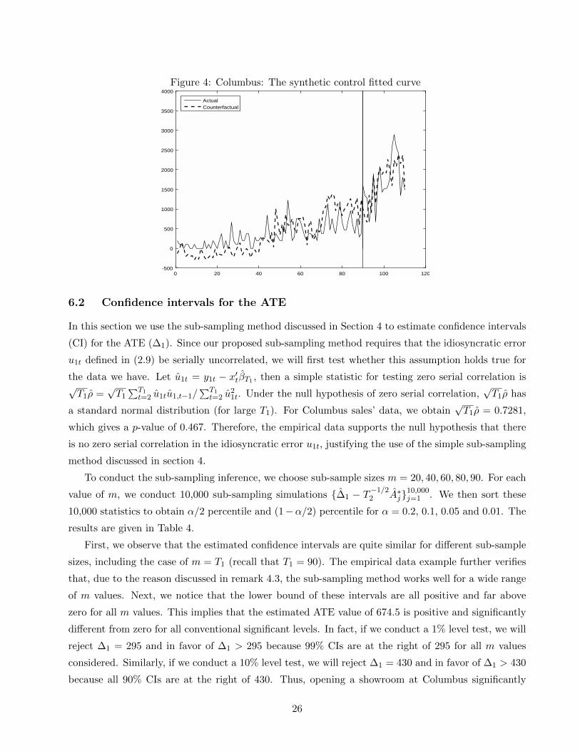
parameters, respectively. Since obviously that opening a showroom has no (or negligible) effects

on z1t, we can use the above model to predict post-treatment counterfactual sale for the treated city.

Specifically, we estimate model (6.1) under the restriction βj ≥ 0 for j ≥ 2 using the pre-treatment data

t = 1, ..., T1 (there is no restriction for other parameters). Let βT1 and γT1 denote the corresponding

estimators. We estimate the counterfactual outcome y01t by y0

1t = x′tβT1 + z′1tγT1 for t = T1 + 1, ..., T

and estimate ATE by T−12

∑Tt=T1+1(y1t − y0

1t).

Figure 7: Columbus: Modified synthetic control ATE, add Covariates

0 20 40 60 80 100 120

0

500

1000

1500

2000

2500

3000

ATEM = 689.98

ATEM(%) = 69.7%



Figure 7 plots the estimation result for Columbus. The ATE becomes 68.7% which is quite close to

the original result of 67%. However, the adjusted R2 decreased slightly from 0.528 to 0.524, indicating

that the three covariates do not have additional explanatory power to explain sale. The virtually same

ATE estimation result with added covariates again supports our original ATE estimation result.

6.3.3 Select control units based on covariate matching

In this subsection we first select cities whose covariates are close to the covariates of the treated city.

Then we select the number of control cities by comparing adjusted R2. Finally we estimate ATE using

the selected control units. We explain this procedure in more details below.

For each j = 1, 2, 3 (corresponding to Unemp, LF, Inc), we regress z1,jt on zi,jt using the pre-

treatment data and obtain the goodness-of-fit R2i,j for i = 2, ..., 11. We obtain a total R-square for city

i by R2i = R2

i,1 +R2i,2 +R2

i,3. We order them in a non-increasing order: R2(2) ≥ R

2(3) ≥ ... ≥ R

2(11). Their

corresponding sales are denoted by y(2),t,...,y(11),t for t = 1, ..., T1. Next, we regress y1t on y(2),t and

obtain an adjusted R2(2); and we regress y1t on (y(2),t, y(3),t) and obtain an adjusted R2

(2),(3); continuing

29

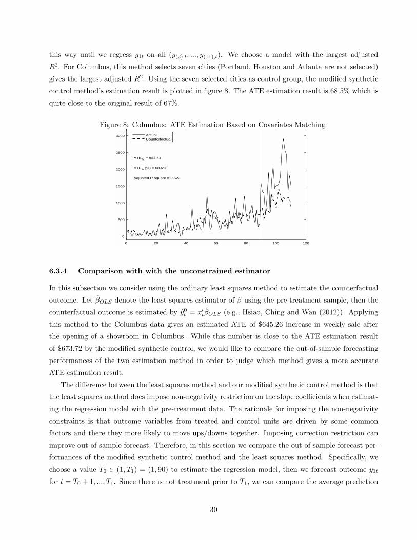
this way until we regress y1t on all (y(2),t, ..., y(11),t). We choose a model with the largest adjusted

R2. For Columbus, this method selects seven cities (Portland, Houston and Atlanta are not selected)

gives the largest adjusted R2. Using the seven selected cities as control group, the modified synthetic

control method’s estimation result is plotted in figure 8. The ATE estimation result is 68.5% which is

quite close to the original result of 67%.

Figure 8: Columbus: ATE Estimation Based on Covariates Matching

0 20 40 60 80 100 120

0

500

1000

1500

2000

2500

3000

ATEM = 683.44

ATEM(%) = 68.5%



6.3.4 Comparison with with the unconstrained estimator

In this subsection we consider using the ordinary least squares method to estimate the counterfactual

outcome. Let βOLS denote the least squares estimator of β using the pre-treatment sample, then the

counterfactual outcome is estimated by y0t = x′tβOLS (e.g., Hsiao, Ching and Wan (2012)). Applying

this method to the Columbus data gives an estimated ATE of $645.26 increase in weekly sale after

the opening of a showroom in Columbus. While this number is close to the ATE estimation result

of $673.72 by the modified synthetic control, we would like to compare the out-of-sample forecasting

performances of the two estimation method in order to judge which method gives a more accurate

ATE estimation result.

The difference between the least squares method and our modified synthetic control method is that

the least squares method does impose non-negativity restriction on the slope coefficients when estimat-

ing the regression model with the pre-treatment data. The rationale for imposing the non-negativity

constraints is that outcome variables from treated and control units are driven by some common

factors and there they more likely to move ups/downs together. Imposing correction restriction can

improve out-of-sample forecast. Therefore, in this section we compare the out-of-sample forecast per-

formances of the modified synthetic control method and the least squares method. Specifically, we

choose a value T0 ∈ (1, T1) = (1, 90) to estimate the regression model, then we forecast outcome y1t

for t = T0 + 1, ..., T1. Since there is not treatment prior to T1, we can compare the average prediction

30

squared error over the period t = T0 + 1, ..., T1. Specifically, we estimate the following model

yt = x′tβ + u1t t = 1, ..., T0 (6.2)

by the modified synthetic control and the least squares method. Let βT0 and βOLS denote the resulting

estimators using the two methods, respectively. We prediction y01t by y0

1t,Msyn = x′tβT0 and y01t,OLS =

x′tβOLS for t = T0 + 1, ..., T1. Then we computet the prediction MSEs by

PMSEMsyn =1

T1 − T0

T1∑t=T0+1

(y1t − y01t,Msyn)2,

PMSEOLS =1

T1 − T0

T1∑t=T0+1

(y1t − y01t,OLS)2.

As suggested in Li and Bell (2017), we consider the cases that the ‘pre-treatment’ estimation

sample is larger than the ‘post-treatment’ evaluation sample. We choose six different values for T0 =

60, 65, 70, 75, 89, 85. The corresponding evaluation sample sizes are T1 − T0 = 30, 25, 20, 15, 10, 5.We report the ratio of PMSE as PMSEOLS/PMSEMsyn. The results are reported in Table 6.

Table 6: Out-of-sample Prediction MSE ratioT0 60 65 70 75 80 85

PMSEOLSPMSEMsyn

1.680 1.104 1.020 1.273 1.188 1.143

From Table 6 we observe that the least squares method has larger PMSE than the modified

synthetic control method for all cases. The PMSE for the former ranges from 2% to 68% larger

than the later. Thus, the empirical example shows that, in order to more accurately predict the

counterfactual outcomes for the treated unit, it is helpful to impose non-negativity restriction on the

slope coefficients when estimating model (6.2).

7 Conclusion

The synthetic control method is a popular and powerful way for estimating average treatment effects.

In this paper we contribute to the theoretical analysis of the synthetic control method. Under the

assumption that there is a long panel data with large pre and post-treatment periods, using the

projection theory, we derive the asymptotic distribution of the synthetic control ATE estimator. The

asymptotic distribution is non-normal and non-standard. Moreover, it is known that the standard

bootstrap method does not work in this case. We resolve the difficulty by proposing an easy-to-

implement sub-sampling method and we establish the validity of sub-sampling method in inferences.

When one only has a long pre-treatment data, but a short post-treatment data, as suggested by

Ferman and Pinto (2016a), Andrews’ (2003) end of sample instability test can be used to test the null

31

hypothesis for a given constant level of treatment effect (∆1t = ∆1,0 for all t = T1 + 1, ..., T ).

We also prove that, when the pre-treatment sample size is large than the number of control units

(i.e., T1 > N − 1), the synthetic control estimator, as a constrained minimization problem, has an

unique solution under a mild condition that the T1 byN data matrix has a full column rank. We further

show the modified synthetic control method suggested by Doudchenko and Imbens (2016) can give

reliable ATE estimation results even when the ”parallel lines” assumption is violated for the standard

synthetic control method. Simulations show that the modified synthetic control method performs

well in practice. Finally, we apply the synthetic control method to a marketing data estimating ATE

of opening a showroom at Columbus by WarbyParker.com. The empirical application demonstrates

that when the standard synthetic control method fits the data poorly, the modified synthetic control

method fits the data well and gives reasonable ATE estimation results.

Appendix A: Uniqueness of the synthetic control estimator

A.1 Assumptions

We first list assumptions that are used in deriving the main results of the paper.

Assumption 1. The data xtTt=1 is a weakly dependent stationary process so that laws of

large number holds: T−11

∑T1t=1 xt

p→ E(xt) and (X ′X/T1) ≡ T−11

∑T1t=1 xtx

′t

p→ E(xtx′t), E(xtx

′t) is

positive definite, where X is the T1 × N matrix with its tth row given by x′t = (1, y2t, ..., yNt). Let

η = limT1,T2→∞√T2/T1, then η is a finite non-negative constant.

Assumption 2. u1tTt=1 is zero mean and serially uncorrelated satisfying T−1/21

∑T1t=1 xtu1t

d→N(0,Σ), where Σ = limT1→∞ T

−11

∑T1t=1

∑T1s=1E(u1tu1sxtx

′s).

Assumption 3. Let v1t = ∆1t−∆1 +u1t, we assume that v1t has zero mean and satisfies a central

limit theorem: T−1/22

∑Tt=T1+1 v1t

d→ N(0,Σ2), where Σ2 = limT2→∞ T−12

∑Tt=T1+1

∑Ts=T1+1E(v1tv1s).

Assumption 4. Let wt = (y1t, y2t, ..., yNt,∆1tdt) for t = 1, ..., T , where dt = 0 if t ≤ T1 and dt = 1

if t ≥ T1 + 1. Assume that wtT1t=1 and wtTt=T1+1 are both weakly stationary processes. Define

ρ(τ) = max1≤t≤T max1≤i,j≤N+1 |Cov(wit, wj,t+τ )/√V ar(wt)V ar(wj,t+τ )|. Then there exits some finite

positive constants C > 0, 0 < λ < 1 such that ρ(τ) < Cλτ .

Assumptions 1 and 2 imply that√T1(βOLS −β0)

d→ N(0, A−1ΣA−1), where A = E(xtx′t) and Σ is

defined in assumption 2. Assumption 3 requires that a central limit theorem applies to a partial sum

of v1t. Assumption 4 is also used in Li and Bell (2017), this assumption ensures that the estimator

βT1 using the pre-treatment data is asymptotically independent with an quantity that involves the

post-treatment sample average of the de-mean treatment effects and the idiosyncratic error.

32

A.2 A projection of the unconstrained estimator

We write the regression model in a matrix form:

Y = Xβ0 + u,

where Y and u are both T1× 1 vectors, X is of dimension T1×N and has a full column rank, β0 is of

dimension N × 1. It is assumed that the true parameter β0 ∈ Λ, where Λ is a closed and convex set

(Λ = ΛSyn or ΛMsyn in our applications).

We denote the constrained least squares estimator as βT1 , i.e.,


(Y −Xβ)′(Y −Xβ) ≡ arg min

β∈Λ‖Y −Xβ‖2,

where ||A||2 = A′A for a vector A.

We denote the unconstrained least squares estimator as βOLS = argminβ∈RN (Y −Xβ)′(Y −Xβ),

i.e., βOLS = (X ′X)−1X ′Y . By the definition of βOLS , we may write

Y = XβOLS + u,

where u = Y −XβOLS . It follows that

f(β)def= ‖Y −Xβ‖2

= ‖X(βOLS − β) + u‖2

= ‖X(βOLS − β)‖2 + 2u′X(βOLS − β) + ‖u‖2

= ‖X(βOLS − β)‖2 + ‖u‖2

≡ (βOLS − β)′X′X(βOLS − β) + ‖u‖2, (A.1)

where the fourth equality follows from u′X = 0 (least squares residual u is orthogonal to X).

Since ‖u‖2 is unrelated to β, the minimizer of f(β) is identical to the minimizer of (βOLS −β)′X′X(βOLS − β). Thus, we have

β = arg minβ∈Λ

(βOLS − β)′X′X(βOLS − β)

= arg minβ∈Λ

(βOLS − β)′(X′X/T1)(βOLS − β)

= arg minβ∈Λ||βOLS − β||2X ,

where the second equality follows since T1 > 0.

33

A.3 The uniqueness of the (modified) synthetic control estimator

We first give the definition of a strictly convex function. A function f is said to be strictly convex if

f(αx+ (1− α)y)) < αf(x) + (1− α)f(y) for all 0 < α < 1 and for all x 6= y, x, y ∈ D, where D is the

domain of f .

Under the assumption that the data matrix XT1×N has a full column rank, we show below that

f(β)def=∑T1t=1(y1t−x′tβ)2 is a strictly convex function. Since the objective function is a convex function

and the constrained domain for β, ΛSyn and Λ are convex sets, then the constrained minimization

problem has an unique (global) minimizer. To see this, we argue by contradiction. Suppose that we

have two local minimizers z1 6= z2. Then for any convex combination z3 = αz1 + (1 − α)z2, we have

f(z3) < αf(z1) + (1 − α)f(z2) for all α ∈ (0, 1). This contradicts the fact that z1 and z2 are two

minimizers. Hence, we must have z1 = z2 and the minimizer is unique.

It remains to show that f(β) defined in (A.1) is a strictly convex function. To see this, letting

A = X′X, then for β, γ ∈ RN with β 6= γ and all α ∈ (0, 1), we have (we ignore the irrelevant constant

term ‖u‖2 in f(β))

f(αβ + (1− α)γ) = (α(βOLS − β) + (1− α)(βOLS − γ))′A(α(βOLS − β) + (1− α)(βOLS − γ))

= α2(βOLS − β)′A(βOLS − β) + (1− α)2(βOLS − γ)

′A(βOLS − γ)

+2α(1− α)(βOLS − β)′A(βOLS − γ)

< α2f(β) + (1− α)2f(γ) + α(1− α)[f(β) + f(γ)]

= αf(β) + (1− α)f(γ),

where the above inequality follows from that A is positive definite and β 6= γ. Hence,

0 < (β − γ)′A(β − γ)

= ((β − βOLS)− (γ − βOLS))′A((β − βOLS)− (γ − βOLS))

= (β − βOLS)′A(β − βOLS) + (γ − βOLS)′A(γ − βOLS)

−2(β − βOLS)′A(γ − βOLS)

= f(β) + f(γ)− 2(βOLS − β)′A(βOLS − γ).

This proves that f(·) is a strictly convex function.

Appendix B: Proofs of Theorems 3.2, 3.3 and 4.1

B.1 Proof of Theorem 3.2

Continuing with the setup in Appendix A, the constrained estimator is defined by


(β − βOLS)′(X ′X/T1)(β − βOLS). (B.1)

34

Thus, βT1 is the projection onto Λ with respect to the norm ‖a‖ =√a′(X ′X/T1)a which is random,

rendering the theory in Fang and Santos (2015) not directly applicable. However, since X ′X/T1p→

E(XtX′t), we will show that one can replace X ′X/T1 by E(XtX

′t) without affecting the asymptotic

results. Define the following “infeasible estimator” (it is infeasible because E(X ′tXt) is unknown in

practice):


(β − βOLS)′E(XtX′t)(β − βOLS) = ΠΛβOLS , (B.2)

where ΠΛ is the projection onto Λ with respect to the norm ‖a‖ =√a′E(XtX ′t)a, i.e.,

ΠΛβ = arg minλ∈Λ

(β − λ)′E(XtX′t)(β − λ) . (B.3)

By Lemma 4.6 of Zarantonello (1971, page 300), see also Proposition 4.1 of Fang and Santos (2015),

we know that

√T1(βT1 − β0) =

√T1(ΠΛβOLS −ΠΛβ0)

=√T1ΠTΛ,β0

(βOLS − β0) + op(1)

= ΠTΛ,β0

√T1(βOLS − β0) + op(1)

d→ ΠTΛ,β0Z1, (B.4)

where the first equality follows from βT1 = ΠΛβOLS and β0 ∈ Λ so that β0 = ΠΛβ0.

In Lemma C.1 of the supplementary Appendix C we show that

βT1 = βT1 + op(T−1/21 ) = ΠΛβOLS + op(T

−1/21 ). (B.5)

Theorem 3.2 follows from (B.4) and (B.5).

We give some explanations of the above derivations. Hilbert Space projection onto convex sets was

studied by Zarantonello (1971) and extended to general econometric modeling settings by Fang and

Santos (2015). The projection operator ΠΛ: RN → Λ (Λ is convex subset in RN ) can be viewed as a

functional mapping. Zarantonello (1971) showed that ΠΛ is (Hadamard) directional differentiable, and

its directional derivative at β0 ∈ Λ is ΠTΛ,β0, the projection onto the tangent cone of Λ at β0. Hence,

the second equality of (B.4) follows from a functional Taylor expansion, the third equality follows from

that TΛ,β0 is positive homogenous of degree one.3 The last line follows from√T1(βOLS − Λβ0)

d→ Z1

and the continuous mapping theorem because projection is a continuous mapping.

We can also see the term ‘tangent cone’ is similar to what we term the derivative of a function at

a given point as a ‘tangent line’ of the function at the given point. Now, the functional derivative of

the mapping ΠΛ is a projection onto the cone ΠTΛ,β0(rather than a line). Therefore, it is called the

‘tangent cone’ of Λ at β0 and is denoted as TΛ,β0 .

3The Projection TΛ,β0 is not a linear operator. However, for α ≥ 0, we have αTΛ,β0 θ = TΛ,β0 α θ for all θ ∈ RN .

35

For readers’ convenience, we give the formal definition of tangent cone of Λ at θ ∈ RN below:

TΛ,θ = ∪α≥0αΛ−ΠΛθ, (B.6)

where for any set A ∈ RN , A is the closure of A.

It can be easily checked that for our synthetic control estimation problem, the tangent cone of Λ

at β0 is the same as the asymptotic range of√T1(βT1 − β0).


First, we write A =√T2(∆1 −∆1) defined in (4.2) as A = A1 + A2, where

A1 = −

1

T2

T∑t=T1+1

x′t

√T2

T1

√T1(βT1 − β0)

A2 =1√T2

T∑t=T1+1

v1t. (B.7)

We know that A2d→ Z2 by assumption 2, where Z2 is distributed as N(0,Σ2) with Σ2 = E(v2

1t).

By Theorem 3.2 and assumption 1, we have A1d→ A1 = −ηE(x′t)ΠTΛ,β0

Z1, where η = limT1,T2→∞√T2/T1

and Z1 is the weak limit of√T1(βOLS − β0).

Also, by Lemma A.1 and Theorem 3.2 of Li and Bell (2016), we know that Z1 and Z2 are asymp-

totically independent with each other, this implies that A1 = −ηE(xt)ΠTΛ,β0Z1 is asymptotically

independent of Z2. Hence, we have

Ad→ −ηE(xt)ΠTΛ,β0

Z1 + Z2. (B.8)


The proof that A∗ can be used to approximate the distribution of A consists of the following arguments.

First, we show that one can consistently estimate Σ2 by Σ2 = 1T2

∑Tt=T1+1 v

21t, where v1t = ∆1t − ∆1.

From ∆1t = y1t−y01t = x′t(β0−βT1)+∆1t+u1t = ∆1t+u1t+Op(T

−1/21 ) and

¯∆1 = x′(β0−βT1)+∆1+u1 =

∆1 +Op(T−1/21 + T

−1/22 ), we have

Σ2 =1

T2

T∑t=T1+1

(∆1t − ∆1)2

=1

T2

T∑t=T1+1

(∆1t + u1t −∆1)2 +Op(T−1/21 + T

−1/22 )

=1

T2

T∑t=T1+1

v21t +Op(T

−1/21 + T

−1/22 )

= Σv +Op(T−1/21 + T

−1/22 ). (B.9)

36

Next, it is obvious that T−1/22

∑Tt=T1+1 v

∗1t

d∼ T−1/22

∑Tt=T1+1 v1t

d→ Z2, where Ad∼ B means that

A and B have the same asymptotic distribution. Hence, to show that the limiting distribution of A∗

defined in (4.3) is the same as that of A, we only need to show that√m(β∗m − βT1)

d∼√T1(βT1 − β0).

To see that this is indeed true, we have

√m(β∗m − βT1) =

√m(β∗m − β0) +

√m(β0 − βT1)

=√m(β∗m − β0) +Op((m/T1)1/2)

d∼√T1(βT1 − β0)

d→ ΠTΛ,β0Z1, (B.10)

where the asymptotic equivalenced∼ follows the facts that

√m(βm − β0) and

√T1(βT1 − β0) have the

same asymptotic distribution, βT1 − β0 = Op(T−1/21 ) and m/T1 = o(1); the last convergence result

follow from Theorem 3.2.

It follows from (B.10) that A∗ defined in (4.3) and A defined in (4.2) have the same asymptotic

distribution. This completes the proof of Theorem 4.1.

37

8 References

Abadie, A. (2005). Semiparametric difference-in-differences estimators. Review of Economic Studies

72, 1-19.

Abadie, A., A. Diamond and J. Hainmueller (2010). Synthetic control methods for comparative

case studies: Estimating the effect of California’s tobacco control program. Journal of the American

Statistical Association 105, 493-505.

Abadie, A. and J. Gardeazabal (2003). The economic costs of conflict: A case study of the Basque

Country. American Economic Review 93, 113-132.

Andrews, D.W.K. 2000. Inconsistency of the bootstrap when a parameter is on the boundary of the

parameter Space. Econometrica 68, 399-405.

Andrews, D.W.K. 2003. End-of-sample instability tests. Econometrica 71, 16611694.

Ashenfelter O (1978) Estimating the Effects of Training Programs on Earnings. The Review of Eco-

nomics and Statistics. 60, 47-57.

Ashenfelter O, Card D (1985) Using the Longitudinal Structure of Earnings to Estimate the Effect of

Training Programs. 1985. The Review of Economics and Statistics. 67, 648-660.

Athey, S., and G. Imbens (2016). The State of Applied Econometrics: Causality and Policy Evaluation.

Working Paper.

Bickel, J.P. and A. Sakov. 2008. On the choice of m in the m out of n bootstrap and confidence

bounds for extrema. Statistica Sinica 18, 967-985.

Bradley, E., Hastie, T., Johnstone, T., and R. Tibshirani (2004). Least Angle Regression. Annals of

Statistics 32, 407-499.

Busse, M., Silva-Risso J, Zettlemeyer F (2006) $ 1,000 Cash Back: The Pass-Through of Auto Manu-

facturer Promotions. The American Economic Review. 96, 1253-1270.

Chevalier, J, Mayzlin D (2006) The Effect of Word of Mouth on Sales: Online Book Reviews. Journal

of Marketing Research. 48, 345-354.

Conley, T.G. and C.R. Taber (2011). Inference with “difference in differences” with a small number

of policy changes. The Review of Economics and Statistics, 93, 113-125.

Doudchenko, N. and G. Imbens (2016). Balancing, regression, difference-in-differences and synthetic

control methods: A synthesis.

Du, Z. and L. Zhang (2015). Home-Purchase Restriction, Property Tax and Housing Price in China:

A Counterfactual Analysis. Journal of Econometrics. 188, 558-568

38

Fang, Z. and A. Santos (2015). Inference on directionally differentiable functions. Under revision for

Review of Economic Studies.

Ferman, B. and C. Pinto (2016a). Inference in Differences-in-difference with Few Treated Groups and

Heteroskedasticity. Unpublished working paper.

Ferman, B. and C. Pinto (2016b). Revisiting the Synthetic Control Estimator. Unpublished working

paper.

Forman C, Ghose A, Goldfarb A (2009) Competition Between Local and Electronic Markets: How the

Benefit of Buying Online Depends on Where You Live. Management Science 55, 47-57.

Goldfarb A, Tucker C (2011) Private Regulation and Online Advertising. Management Science. 57,

40-56.

Hahn, J. and R. Shi (2016). Synthetic Control and Inference. Unpublished working paper.

Hsiao, C., Ching, H.S. and S.K. Wan (2012). A panel data approach for program evaluation: Measuring

the benefit of political and economic integration of Hong Kong with mainland China. Journal of

Applied Econometrics 27, 705-740.

Hong, H. and J. Li 2017. The Numerical Delta Method and Bootstrap Unpublished working paper.

Li, K. and D. Bell. 2017. Estimation of average treatment effects with panel data: asymptotic theory

and implementation. Journal of Econometrics 197, 65-75.

Mantin, B. and E. Rubin. 2016. Fare Prediction Websites and Transaction Prices: Empirical Evidence

from the Airline Industry Marketing Sciences 35, 640-655.

Ozturk, O.C., S. Venkataraman and P. K. Chintagunta. 2016. Price Reactions to Rivals Local Channel

Exits Marketing Sciences 35, 588604.

Politis, D.N., J.P. Romano and M. Wolf. 1999. Sub-sampling. Springer.

Wang, K. and A. Goldfarb. 2017. Can offline stores drive online sales? forthcoming in Journal of

Marketing Research

Zarantonello, E.H. (1971). Projection on convex sets and Hilbert Spaces and spectral theory. In

Contributions to Nonlinear Functional Analysis (E.H. Zarantonello ed.). Academic Press.

39

Supplementary Appendix C: Two useful lemmas

In this supplementary appendix we prove two lemmas that are used to prove Theorem 3.2.

Lemma C.1 Under the same conditions as in Theorem 3.2, we have

βT1 = βT1 + op(T−1/21 ) = ΠΛβOLS + op(T

−1/21 ).

Proof: For any fixed ε > 0, suppose that√T1‖βT1 − βT1‖ > ε, then we have

√T1(βT1 − βOLS)′(X ′X/T1)

√T1(βT1 − βOLS) <


√T1(βT1 − βOLS) , (C.1)

where the strict inequality is due to uniqueness of the projection and the assumption that ε > 0 which

implies that βT1 6= βT1 . By simple algebra (adding/subtracting terms), we have:


√T1(βT1 − βOLS)

=√T1(βT1 − βT1 + βT1 − βOLS)′(X ′X/T1)

√T1(βT1 − βT1 + βT1 − βOLS)

=√T1(βT1 − βOLS)′(X ′X/T1)

√T1(βT1 − βOLS)

+√T1(βT1 − βT1)′(X ′X/T1)

√T1(βT1 − βT1)

+2√T1(βT1 − βOLS)′(X ′X/T1)

√T1(βT1 − βT1). (C.2)

By (C.1) and (C.2) we know that the sum of the last two terms in (C.2) is negative, i.e.,

DT1

def=

√T1(βT1

− βT1)′(

1

T1X ′X

)√T1(βT1

− βT1) + 2

√T1(βT1

− βOLS)′(

1

T1X ′X

)√T1(βT1

− βT1)

≡ D1,T1 +D2,T1 < 0. (C.3)

Let SN = a ∈ RN : ‖a‖ = 1, the unit sphere in RN , we have:

D1,T1 =√T1(βT1 − βT1)′

(1

T1X ′X

)√T1(βT1 − βT1)

= ‖√T1(βT1

− βT1)‖2[ √

T1(βT1− βT1

)′

‖√T1(βT1 − βT1)‖

(1

T1X ′X

) √T1(βT1

− βT1)

‖√T1(βT1 − βT1)‖

]

≥ T1‖βT1 − βT1‖2 infa∈SN

a′(

1

T1X ′X

)a

= T1‖βT1− βT1

‖2λmin

(1

T1X ′X

)≥ ε2λmin

(1

T1X ′X

)p→ ε2λmin[E(XtX

′t)] > 0 , (C.4)

40

because√T1‖βT1 − βT1‖ ≥ ε and E(XtX

′t) is nonsingular, where λmin(A) denotes the minimum

eigenvalue of a square matrix A, the third equality used Lemma C.2 which is proved at the end of this

Appendix.

By writing (X ′X/T1) = E(XtX′t)+(X ′X/T1)−E(XtX

′t), the second term in (C.3) can be rewritten

as:

D2,T1 = 2√T1(βT1 − βOLS)′(X ′X/T1)

√T1(βT1 − βT1)

= 2√T1(βT1 − βOLS)′[E(XtX

′t)]√T1(βT1 − βT1)

+2√T1(βT1 − βOLS)′(X ′X/T1 − E[XtX

′t])√T1(βT1 − βT1)

= 2√T1(βT1 − βOLS)′[E(XtX

′t)]√T1(βT1 − βT1) + op(1) , (C.5)

where we used the fact that√T1(βT1 − βT1) = Op(1) because:

‖√T1(βT1 − βT1)‖ ≤ ‖

√T1(βT1 − β0)‖+ ‖

√T1(βT1 − β0)‖

= ‖√T1(ΠΛ,T1 βOLS − β0)‖+ ‖

√T1(ΠΛβOLS − β0)‖

≤√T1‖βOLS − β0‖T1 +

√T1‖βOLS − β0‖ = Op(1) ,

where we used the Lipschitz continuity of projection operators (Zarantonello, 1971; p.241, first display

in equation (1.8)), and ΠΛ,T1 is the projection onto Λ with respect to the aforementioned random

norm ‖a‖T1 =√a′(X ′X/T1)a.

Also, by the definition of βT1 and Lemma 1.1 in Zarantonello (1971, page 239),

√T1(βT1 − βOLS)′[E(XtX

′t)]√T1(βT1 − βT1) ≥ 0 . (C.6)

Combining (C.3), (C.4), (C.5) and (C.6), we know that

√T1(βT1 − βOLS)′[E(XtX

′t)]√T1(βT1 − βT1) = op(1). (C.7)

Thus, we have shown that: if√T1‖βT1 − βT1‖ > ε, then

√T1(βT1

− βOLS)′(

1

T1X ′X

)√T1(βT1

− βOLS)−√T1(βT1

− βOLS)′(

1

T1X ′X

)√T1(βT1

− βOLS)

= DT1< 0, (C.8)

which implies that (if A implies B, then P (A) ≤ P (B))

P (√T1‖βT1 − βT1‖ > ε) ≤ P (DT1 < 0)

≤ P (op(1) + ε2λmin

(1

T1X ′X

)< 0)

→ P (ε2λmin(E(XtX

′t))≤ 0) = 0. (C.9)

41

Equation (C.9) is equivalent to βT1 − βT1 = op(T−1/21 ), or

βT1 = ΠΛ,T1 βOLS + op(T−1/21 ) . (C.10)

This finishes the proof of Theorem 3.2.

Lemma C.2 Let A be an N ×N positive definite matrix, SN = a ∈ RN : ‖a‖ = 1, the unit sphere

in RN , then we have infa∈SN a′Aa = λmin(A) .

Proof: Let v1, ..., vN be N eigen-vectors of A with corresponding eigen-values λ1, ..., λN so that Avj =

λjvj for j = 1, ..., N . Then since v1, ..., vN form an orthonormal base for SN , we have for any a ∈ SN ,

a =∑Ni=1 civi with

∑Ni=1 c

2i = 1 since a′a = 1 and v′ivj = δij (the Kronecker delta). Then we have

a′Aa =N∑i=1

N∑j=1

civ′iAcjvj

=N∑i=1

N∑j=1

civ′icjAvj

=N∑i=1

N∑j=1

cicjλjv′ivj

=N∑i=1

λjc2j

≥ λmin

N∑j=1

c2j

= λmin, (C.11)

which implies (i) infa∈SN a′Aa ≥ λmin.

On the other hand, pre-multiplying Avj = λjvj by v′j , we get λj = v′jAvj ≥ infa∈SN a′Aa for all

j = 1, ..., N , which implies (ii) λmin ≥ infa∈SN a′Aa. Combining (i) and (ii) we finish the proof of

Lemma C.2.

Supplementary Appendix D: Asymptotic theory with trend station-

ary data

Asymptotic theory for the unconstrained estimator

In this section, we derive the asymptotic distribution of the ATE estimator ∆1 defined in (3.9). For

the post-treatment, we have y11t = y0

1t + ∆1t. Hence, we have for t = 1, ..., T ,

y1t = αt+ z′tβ + dt∆1t + v1t, (D.1)

42

where dt = 0 for t ≤ T1 and dt = 1 for t ≥ T1 + 1.

Let α and β be the least squares estimators of α and β based on (3.8). Then it is well established

that (e.g., Hamilton (1994), Chapter 16) α − α = Op(T−3/21 ) and β − β = Op(T

−1/21 ). Thus, using

(3.9) and (D.1) we have

∆1 −∆1 =1

T2

T∑t=T1+1

[y1t − y0

1t

]−∆1

= − 1

T2

T∑t=T1+1

[(αT1 − α0)t− z′t(βT1 − β0) + ∆1t −∆1 + v1t

]

= −[

2T1 + T2 + 1

2

](α− α)− [E(z′t) + op(1)](β − β) +

1

T2

T∑t=T1+1

v1t, (D.2)

where we used∑Tt=T1+1 t = (T1 + 1 + T )T2/2 = (2T1 + T2 + 1)T2/2, v1t = ∆1t −∆1 + u1t.

Hence,

√T2(∆1 −∆1) = −

√T2/T1

[2 + T2/T1

2

]√T 3

1 (αT1 − α0)−√T2/T1E(z′t)

√T1(βT1 − β0)

+1√T2

T∑t=T1+1

v1t + op (1)

= −(√

T2/T1(2 + T2/T1)/2 ,√T2/T1E(z′t)

)(√T 3

1 (αT1 − α0)√T1(βT1 − β0)

)

+1√T2

T∑t=T1+1

v1t + op(1)

= −c′MT1(γT1 − γ0) +1√T2

T∑t=T1+1

v1t + op(1), (D.3)

where c = (√η(2 + η)/2,

√ηE(z′t))

′, η = limT1,T2→∞ T2/T1, γT1 = (αT1 , β′T1

)′ and γ0 = (α0, β′0)′,

MT1 =√T1diag(T1, 1, ..., 1) which is an (N + 1) × (N + 1) diagonal matrix with the first diagonal

element equals to T3/21 and all other diagonal elements equal to

√T1.

To establish the asymptotic distribution of√T2(∆1 −∆1), we make the following assumptions.

Assumption D1. Let zt = (1, y∗′

2t, ..., y∗Nt)′. We assume that (i) ztTt=1 is a weakly dependent

and weakly stationary process, T−11

∑T1t=1 ztz

′tp→ E(ztz

′t) as T1 → ∞, and [E(ztz

′t)] is invertible; (ii)

MT1(γOLS − γ)d→ N(0,Ω) , where Ω is a positive definite matrix.

Assumption D2. Let v1t = ∆1t −∆1 + v1t. Then T−1/22

∑Tt=T1+1 v1t

d→ N(0,Σ2) as T2 →∞, where

Σ2 = limT2→∞ T−12

∑Tt=T1+1

∑Ts=T1+1E(v1tv1s) is the asymptotic variance of T

−1/22

∑Tt=T1+1 v1t.

Assumption D3. Let wt = (v1t, y∗2t, ..., y

∗Nt)′. We assume that wt is a ρ-mixing process with the

mixing coefficient ρ(τ) satisfies the condition: ρ(τ) ≤ C λτ for some finite positive constants C > 0

and 0 < λ < 1, where ρ(τ) = max1≤i,j≤N |Cov(wit, wj,t+τ )|/√V ar(wit)V ar(wj,t+τ ), wit is the ith

43

component of wt for i = 1, ..., N .

Assumptions D1 and D2 are not restrictive. They require that (zt, v1t) to be a weakly dependent

stationary process so that law of large numbers and central limit theorem hold for their (partial) sums.

If E(ztz′t) is not invertible, we can remove the linearly dependent regressors and redefine zt as a subset

of (1, y∗2t, ..., y∗Nt)′ such that assumption 1 holds. Assumption D3 further imposes an exponential decay

rate for the ρ-mixing processes. Many ARMA processes are known to be ρ-mixing with exponential

decay rate.

By Assumption D3 and the proof of Theorem 3.2 and Lemma 1 in Li and Bell (2017), we know that

γ−γ is asymptotic independent with T−1/22

∑Tt=T1+1 v1t. Therefore, applying the projection theory to

(D.3) we immediately have the following result.

Under assumptions D1 to D3 and note that γ0 ∈ Λ, we have

√T2(∆1 −∆1) = −c′MT1(γT1 − γ0) +

1√T2

T∑t=T1+1

v1t + op(1)

= −c′MT1(ΠΛγOLS −ΠΛγ0) +1√T2

T∑t=T1+1

v1t + op(1)

= −c′ΠTΛ,γ0MT1(γOLS − γ0) +

1√T2

T∑t=T1+1

v1t + op(1)

d→ −c′ΠTΛ,γ0Z3 + Z2, (D.4)

where Z3 is the weak limit ofMT1(γOLS−γ0) as described in Assumption C1, Z2 is independent with Z3,

and is normally distributed with a zero mean and variance Σ2 = limT2→∞ T−12

∑Tt=T1+1

∑Ts=T1+1E(v1tv1s).

Supplementary Appendix E: Explanation of sub-sampling method

works for a wide range of sub-sample sizes

In this appendix, we explain why the sub-sampling method works well for our estimated ATE estimator

for a wide range of sub-sample size m values.

E.1 A simple example from Andrews (2000)

We consider a simple example as considered in Andrews (2000) where Yi, for i = 1, ..., n, is iid

N(µ0, 1) with µ0 ≥ 0, i.e., Yi = µ0 + ui with ui iid N(0, 1) and that µ0 ∈ Λ = R+ def= y : y ≥ 0.

The constrained least squares estimator of µ0 is µn = maxYn, 0, where Yn = n−1∑ni=1 Yi. It is easy

to show that

Sndef=√n(µn − µ0)

d→Z if µ0 > 0

maxZ, 0 if µ0 = 0,(E.1)

44

where Z denotes a standard normal random variable. Let Y ∗i be random draws from Yjnj=1, then

a bootstrap analogue of (E.1) is√n(µ∗n − µn), where µ∗n = maxY ∗n , 0, where Y ∗n = n−1∑n

i=1 Y∗i .

Andrews (2000) show that this standard resampling bootstrap method as well as several parametric

bootstrap methods do not work in the sense that when µ0 = 0, S∗n =√n(µ∗n− µn) will not converge to

maxZ, 0, the limiting distribution of Sn. In fact, Andrews shows that S∗n converges to a distribution

that is to the left of maxZ, 0.Andrews (2000) also suggests a few re-sampling methods that overcome the problem. One partic-

ular easy-to-implement method is a parametric sub-sampling method. Specifically, for m satisfies that

m→∞ and m/n→ 0 as n→∞, one can use S∗m =√m(µ∗m− µn) to approximate the distribution of

√n(µn − µ0), where µm = maxY ∗m, 0, Y ∗m = m−1∑m

i=1 Y∗i with Y ∗i is iid draws from N(Yn, 1), i.e.,

Y ∗i = Yn + u∗i with u∗i iid N(0, 1). To see that the sub-sampling method indeed works, we have that,

conditional on Yini=1,

S∗mdef=√m(µ∗m − µn)

= max√

mY ∗m, 0−√mµn

= max√

mY ∗m, 0−√mµ0 −

√m(µn − µ0)

= max√

m(Y ∗m − Yn + Yn − µ0),−√mµ0

−√m(µn − µ0)

= max

√m(Y ∗m − Yn) +

√m/n√n(Yn − µ0),−

√mµ)

−√m/n√n(µn − µ0)

= max√

m(Y ∗m − Yn) + op(1),−√mµ0

+ op(1)

d→Z if µ0 > 0

max Z, 0 if µ0 = 0,(E.2)

where the second equality follows from the definition of µ∗m, we add/subtract√mµ0 at the third

equality, the fourth equality follows from maxa, b− c = maxa− c, b− c, the sixth equality follows

from m/n = o(1),√n(Yn−µ0) = Op(1) and o(1)Op(1) = op(1). The last equality follows from the fact

that Y ∗i − Yn = u∗i is iid N(0, 1). Hence,√m(Y ∗m − Yn)

d∼ N(0, 1) ≡ Z for any value of m. If Y ∗i mi=1

is iid with mean Yn and unit variance but is not normally distributed, then we need m to be large so

that√m(Y ∗m − Yn)

d→ N(0, 1) ≡ Z by virtue of a central limit theorem argument (as m→∞).

Comparing (E.1) and (E.2), we see that sub-sampling method works under very mild conditions

that m→∞ and m/n→ 0 as n→∞.

E.2 Testing zero ATE by sub-sampling method

We conduct simulations to examine the finite sample performances of the sub-sampling method. We

generate Yi iid N(0, 1) (i.e., µ0 = 0) for i = 1, ..., n and we choose n = 100 and conduct 5000

simulations. Within each simulation, we generate 2000 sub-sampling samples with sub-sample sizes

m ∈ 5, 10, 20, 30, 50, 100. Note that we select the largest m = n = 100 because we want to show

45

numerically that the standard bootstrap method does not work. For each fixed value of m, we sort the

2000 sub-sampling statistics in an ascending order such that S∗m,(1) ≤ S∗m,(2) ≤ ... ≤ S

∗m,(2000), then we

get right-tail α-percentile value by S∗((1−α)(2000)). We record rejection rate as the percentage that S is

greater or equal to S∗((1−α)(2000)) for α ∈ 0.01, 0.05, 0.1, 0.2. We consider two cases: (i) We generate

Yi iid N(0, 1) and Y ∗i = Yn + vi with vi iiid N(0, 1); and (ii) We generate Yi uniformly distributed

over [−√

3,√

3] (so that it has zero mean and unit variance) and Y ∗i = Yn + vi with vi iid uniformly

distributed over [−√

3,√

3]. The results for the two cases are almost identical. To save space we only

report are reported the normally distributed vi in Table 7.

Table 7: Estimated sizes (Y ∗i ∼ N(Yn, 1))

m=5 m=10 m=20 m=30 m=50 m=100

1% .0132 . 0126 .0124 .0130 .0136 .0248

5% .0516 .0518 .0518 .0532 .0658 .1032

10% .0960 .0968 .1006 .1104 .1346 .2014

20% .1936 .2004 .2278 .2588 .3164 .4020

First, we see that the sub-sampling method with 5 ≤ m ≤ 20 seem to work well. Second, we

see clearly that using m = n or m close to n (m ≥ 50) do not work. For example, when m = n, it

gives estimated rejection rates double that of the nominal levels. Andrews (2000) showed that the

distribution of√n(µ∗n−µn) is to the left of that of

√n(µn−µ0). Hence, the bootstrap method will lead

to over rejection of the null hypothesis. Our simulation results verifies Andrews’ theoretical analysis.

The simulation results seem to be in contradiction to the simulation results reported in Section

5 where even for m = n, the sub-sampling method seems to be fine. We explain the seemingly

contradictory results in the next subsection.

E.3 Not all parameters are at the boundary

Our simulations reported in Section 5 corresponds to the case of β0,j > 0 for j = 2, ..., 7 and β0,j = 0

for j = 8, ..., 11. The constrained estimators βT1,j (β∗m,j) for j = 8, 9, 10, 11 can cause problems for the

standard bootstrap method not to work. However, notice that our ATE estimator also depends on

βT1,j (β∗m,j) for j = 1, ..., 7 which does not take the one-dimensional problem boundary value 0. This

helps to improve sub-sampling method for large value of m. More importantly, our ATE estimator also

contains a term not related to βT1 (see the second term at the right hand side of (4.5)) and the existence

of this term further improves the performance of the sub-sampling method when m is close to or equal

to n. This is the reason why in our simulations even when m = n the sub-sampling method seems

to work fine. To numerically verify this conjecture, we generate a sequence of iid Z1, Z2 ∼ N(0, σ2v)

random variables and add them to Sn and S∗m, i.e., Sn = Sn +Z1 and S∗m = S∗m +Z2, we then repeat

the simulations to compute the estimated sizes. The results for σv = 1 and 5 are reported in Table

8. We observe the performance of the sub-sampling statistic S∗m improves significantly over S∗m for

46

m = 50 and 100. Consider the case of σv = 1 and m = n, the rejection rates based on S∗m is about

20% higher than that of the nominal levels whereas it was 100% higher than that of nominal levels

based on S∗m.

From Table 8 we see that when σ2v is large, Z1 and Z2 becomes the dominating components of Sn

and S∗m, therefore, the sub-sampling method works well for all values of m including m = n. Also

note that the estimated sizes for σ2v = 1 only slightly over sized compared to σ2

v = 25 shows that the

significant improvements in the estimated sizes (over the case of σ2v = 0) does not require adding a

regular component with large dominating variance.

Table 8: Estimated sizes: Adding a N(0, σ2v) to Sn and S∗m

m=5 m=10 m=20 m=30 m=50 m=100

σv = 1

1% .0104 .0110 .0112 .0128 .0122 .0114

5% .0550 .0562 .0562 .0590 .0600 .0648

10% .1066 .1098 .1140 .1168 .1198 .1236

20% .2170 .2244 .2320 .2372 .2440 .2520

σv = 5

1% .0112 .0116 .0116 .0110 .0124 .0128

5% .0518 .0521 .0528 .0530 .0542 .0556

10% .1030 .1044 .1046 .1048 .1060 .1074

20% .2070 .2082 .2030 .2102 .2126 .2160

47

Date post:	25-Feb-2022
Category:	Documents
Upload:	others
View:	3 times
Download:	0 times

Estimating Average Treatment E ects Using a Modi ed ...

Documents