29
Estimating Causal Effects from Observations Advanced Data Analysis from an Elementary Point of View
| Date post: | 12-Feb-2017 |
| Category: |
Data & Analytics |
| Upload: | antigoni-maria-founta |
| View: | 20 times |
| Download: | 1 times |

Estimating Causal Effects from
Observations
Advanced Data Analysisfrom an Elementary Point of View

Credits TeamThe slides below are derived from the Chapter 27 of the book “Advanced Data Analysis from an Elementary Point of View“ by Cosma Shalizi of the Carnegie Mellon University, which was created in order to assist the “Advanced Data Analysis” course of the CMU.
Antigoni-Maria Founta, UIM: 647
Ioannis Athanasiadis, UIM: 607

OverviewIdentification & Estimation
➔ Back-door Criteria & Estimators◆ Estimating Average Causal Effects◆ Avoiding Estimating Marginal Distributions◆ Matching◆ Propensity Scores◆ Propensity Score Matching
➔ Instrumental Variables Estimates
Conclusion
➔ Uncertainty & Inference➔ Comparison of Methods

Identification of Causal Effects
● Causal Conditioning: Pr(Y|do(X = x))
//Counter-factual, not always identifiable even if X & Y are observable
● Probabilistic Conditioning: Pr(Y|X = x)
//Factual, always identifiable if X & Y are observable
Our goal is to identify when quantities like the former are functions of the distribution of observable variables!And once identified, the next question is how we can actually estimate it...

Identification/Estimation of Causal Effects
Each one of the next techniques provides us with both identification of causal effects as well as formulas to estimate them:
1. Back-door Criterion
2. Front-door Criterion
3. Instrumental Variables
* Since estimating with the front-door criterion amounts to doing two rounds of back-door adjustment, we will continue this lecture working only with the back-door criterion.
*

Back-door Criteria Estimations

Back-door criterion
CRITERIA:
I. S blocks every back-door path between X and Y II. No node in S is a descendant of X
S is each subset that meets the back-door criteria.
E.g.● S={S1,S2} or S={S3} or
S={S1,S2,S3} meet criteria● S={S1} or S={S2} or S={S3,B}
fail the criteria
Back-door Criteria Formula
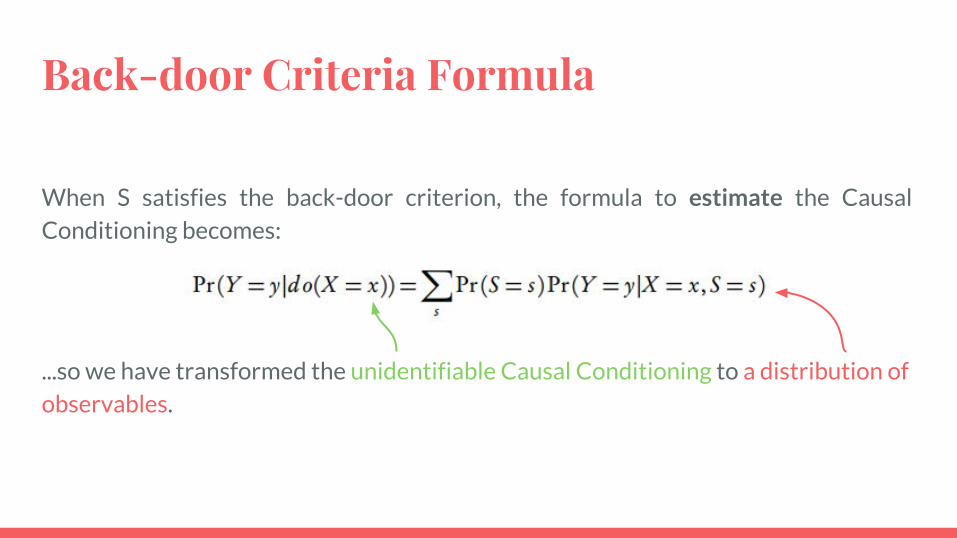
When S satisfies the back-door criterion, the formula to estimate the Causal Conditioning becomes:
...so we have transformed the unidentifiable Causal Conditioning to a distribution of observables.
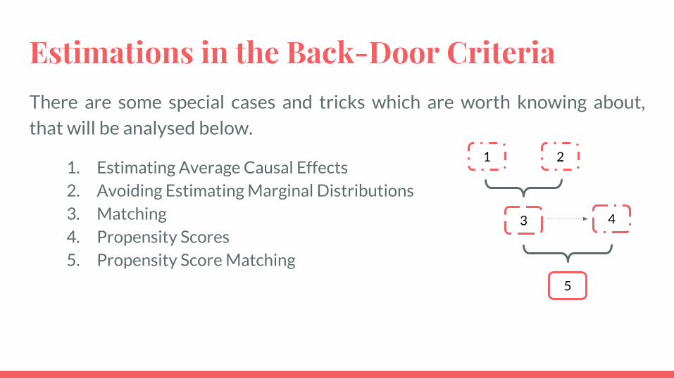
Estimations in the Back-Door CriteriaThere are some special cases and tricks which are worth knowing about,
that will be analysed below.
1. Estimating Average Causal Effects2. Avoiding Estimating Marginal Distributions3. Matching4. Propensity Scores5. Propensity Score Matching
1 2
3 4
5
1. Estimating average causal effects I
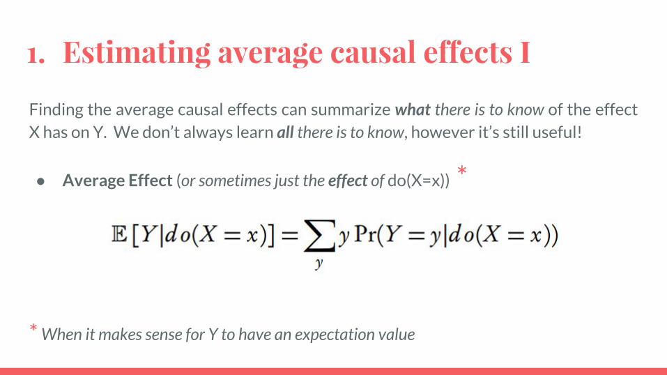
Finding the average causal effects can summarize what there is to know of the effect X has on Y. We don’t always learn all there is to know, however it’s still useful!
● Average Effect (or sometimes just the effect of do(X=x)) *
* When it makes sense for Y to have an expectation value

1. Estimating average causal effects II
● If we apply the Back-Door Criterion Formula with control variables S:
=>
µ(x, s)
(Inner Conditional Expectation => Regression Function)
We can compute µ(x, s) but we still need to know Pr(S=s)...

2. Avoiding Estimating Marginal Distributions● The demands for computing, enumerating and summarizing the various
distributions of the Back-Door Criteria Formula is very high, so we need to reduce these burdens. One shortcut is to smartly enumerate the possible values of S.
● How? Law of Large Numbers!
With a large sample:

3. Matching (Binary Levels)Combination of the above methods:
● By the Estimation of Average Causal Effects we got:
E [Y|do(X=x)] = ΣPr(S=s)µ(x, s)
● By the Law of Large Numbers we got:
E [Y|do(X=x)] = 1/n Σ Pr(Y=y | X = x, S = si)
When the variable is binary, we are interested in the expectations of X=0 or 1.So we want the difference: E [Y|do(X=1)] - E [Y|do(X=0)]
This is called Average Treatment Effect or ATE!
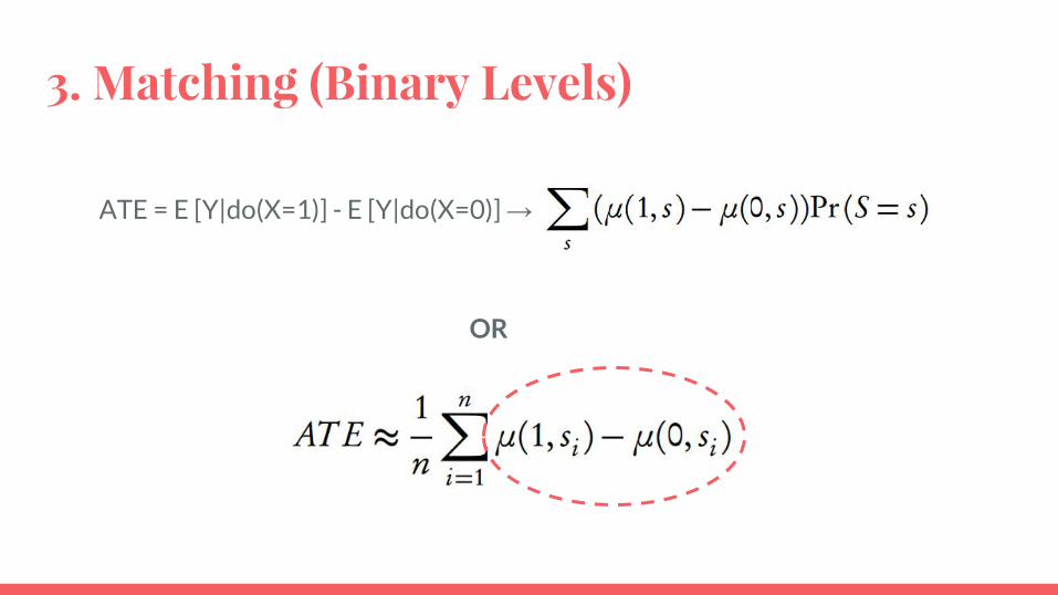
3. Matching (Binary Levels)
ATE = E [Y|do(X=1)] - E [Y|do(X=0)] →
OR
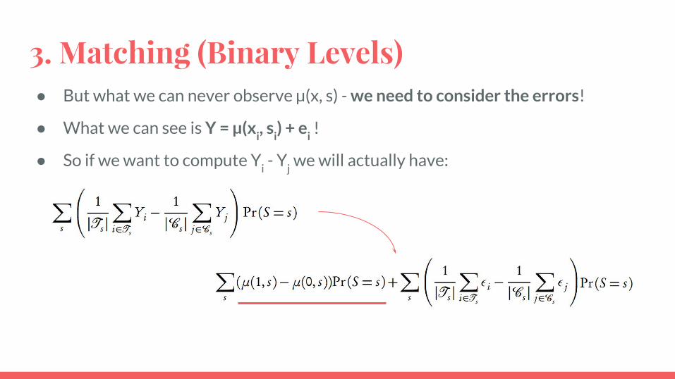
3. Matching (Binary Levels)● But what we can never observe µ(x, s) - we need to consider the errors!
● What we can see is Y = µ(xi, s
i) + e
i !
● So if we want to compute Yi - Y
j we will actually have:

3. Matching (Binary Levels)If we make an assumption that there is an s whose value is the same for two units i and i*, where X=0 and X=1, then we can say that:
So, if we can find a match i* for every unit i, then:
Matching works vastly better than estimating μ through a linear model!

3. Matching (Binary Levels) - ConclusionMatching is really just Nearest Neighbor Regression!
● Many technicalities arise. What if we match a unit against multiple units / we can’t find exact match?If not an exact match -> match each treated unit against the control-group unit with the closest values of the covariates.
● Matching does not solve the identification problem. We need S to satisfy the back-door criterion!
● As any NN method, many issues arise. Fixed K → low bias, but not always what we want. Prioritizing low bias is not always a good idea.
Bias - Variance tradeoff is a tradeoff!
4. Propensity Scores● Curse of dimensionality over data or conditional distributions is actually
manageable if control variables have few dimensions.
● If R, S sets of control variables, both satisfy back-door criterion and have all else equal but dimensions, we should choose the one with the fewer variables (e.g. R).
● Especially when we can say that R = f(S): if S satisfies the back-door criterion, then so does R. Since R is a function of S, both the computational and the statistical problems which come from using R are no worse than those of using S, and possibly much better, if R has much lower dimension.

4. Propensity Scores● All that is required is that some combinations of the variables in S carry the same
information about X as the whole of S does - summary score!
● We (hope we) can reduce a p-dimensional set of control variables to a one-dimensional set.
● In reality that is difficult as it depends on the functional form a non-parametric case. However, there is a special case where we can possibly use one-dimensional summary;when X is binary! So in that case:
Propensity score: f(S) = Pr(X=1|S=s), which is our summary R
● However, still no analytical formula for f(S) so it needs to be modeled and estimated. The most common model used is Logistic Regression, but in a high-dimensional S that would also suffer from curse of dimensionality.

5. Propensity Score Matching● Even if X is a binary variable, if S suffers from high dimensions then matching is
a really tough task → the more the levels of S variables, the lower the matching.
● Solution: Matching on R = f(S) - propensity scores!
● The gain here is in computational tractability and (perhaps) statistical efficiency, not in fundamental identification. Que sera, sera…
Incredibly popular method ever since, huge number of implementations.

OverviewIdentification & Estimation
➔ Back-door Criteria & Estimators◆ Estimating Average Causal Effects◆ Avoiding Estimating Marginal Distributions◆ Matching◆ Propensity Scores◆ Propensity Score Matching
➔ Instrumental Variables Estimates
Conclusion
➔ Uncertainty & Inference➔ Comparison of Methods

Instrumental Variables

Instrumental Variables● I is an instrument for identifying the effect of X on Y if:
○ I is a cause of X
○ I is associated to Y only through X
○ Given some controls S, I is a valid instrument when every path from I to Y left open by S has an
arrow into X
● Change one-unit in I → changes α-unit in X → changes αβ-unit in Y
● So, β is the way for us to estimate the causal coefficient of X on Y!
● We need to estimate β so that we satisfy all the above criteria. However, things get very complicated when we care about many instruments and/or interest about causal of multiple variables.

Instrumental Variables● In general, we need two steps * //2-stage Regression / 2-stage Least Squares
1. Regress X on I and S. Call the fitted values xˆ.//We see how much changes in the instruments affect X.
2. Regress Y on xˆ and S, but not on I. The coefficient of Y on xˆ is a consistent estimate of β.//We see how much these I-caused changes in X change Y
● In the simplest case, when everything is linear, the above procedure is calculated by the Wald estimator:
* This works, provided that the linearity assumption holds.

Instrumental Variables● There are circumstances where it is possible to use instrumental variables in
nonlinear and even nonparametric models, BUT the technique becomes far more complicated.
● Solving integral equations like this:
It is not impossible, BUT it’s painful :-(
The techniques needed are really complicated.

OverviewIdentification & Estimation
➔ Back-door Criteria & Estimators◆ Estimating Average Causal Effects◆ Avoiding Estimating Marginal Distributions◆ Matching◆ Propensity Scores◆ Propensity Score Matching
➔ Instrumental Variables Estimates
Conclusion
➔ Uncertainty & Inference➔ Comparison of Methods
Uncertainty & InferenceWe can reduce the problem of causal inference → ordinary statistical inference.
So, in general, with the use of analytical formulas we can assess our uncertainty about any of our estimates of causal effects the same way we would assess any other statistical inference (e.g. standard errors).
However, in the two-stage least squares, taking standard errors, etc for β from the
usual formulas for the second regression neglects the fact that this estimate of β comes from regressing Y on x, which is it itself an estimate and so uncertain.

Comparison of Methods
Matching Instrumental Variables
(+) Clever
(-) Assumptions on underlying DAG
Crucial PointThe covariates block all
back-door pathways between X and Y.
The instrument is an indirect cause of Y, but only through X (no other
unblocked paths connecting I & Y).
Covariates used in matching are not enough to block all the
back-door paths.
Too quick to discount the possibility that the instruments are connected to
Y through unmeasured pathways.
According to Practitioners:

Thank You!


