Estimating Contract Indexation in a Financial Accelerator ... · se issues are pursued wtihn ti he...

Research Papers

Estimating Contract Indexation in a Financial Accelerator ModelCharles T. CarlstromTimothy S. FuerstAlberto OrtizMatthias PaustianJune 2013

10

Estimating ContraCt indExation in a FinanCial aCCElErator modEl

authors:Charles T. Carlstrom Timothy S. Fuerst Alberto OrtizMatthias Paustian

© 2013 Center for Latin American Monetary Studies (cemla) Durango 54, Colonia Roma Norte, Delegación Cuauhtémoc, 06700 México D.F., México. E-mail:[email protected]://www.cemla.org The views expressed in this paper are those of the authors, and not necessarily those of the Bank of England, the Center for Latin American Monetary Studies, the Federal Reserve Bank of Cleveland, or of the Board of Governors of the Federal Reserve System or its staff.

Research Papers

10

CEMLA | Documentos de Coyuntura 5 | Febrero de 2015

Estimating Contract Indexation in a Financial Accelerator Model

Charles T. CarlsTrom, Federa l Reser ve Bank of C leve land T imoThy s. FuersT, Univers i t y o f Notre Dame Federa l Reser ve Bank of C leve landalberTo orTiz, cem l a and egade Bus iness Schoo l maTThias PausTian, Bank of Eng land

abstraCt

[email protected] [email protected] [email protected] [email protected]

this degree of indexation, (3) the importance of investment shocks in the business cycle depends upon the estimated level of indexation, and (4) although the data prefers the fi-nancial model with indexation over the frictionless model, they have remarkably similar business cycle properties for non-financial exogenous shocks.

cemla | Research Papers 10| June 2013

This paper addresses the positive implications of inde-xing risky debt to observable aggregate conditions. The-se issues are pursued within the context of the celebrated financial accelerator model of Bernanke, Gertler and Gil-christ (1999). The principle conclusions include: (1) the estimated level of indexation is significant, (2) the business cycle properties of the model are significantly affected by

JEL Codes: E32, E44.

Keywords: Agency costs; financial accelerator; busi-ness cycles.

1

2 CEMLA | Research Papers 10 | June 2013

1. INTRODUCTION

he fundamental function of credit markets is to channel funds from savers to

entrepreneurs who have some valuable capital investment project. These efforts

are hindered by agency costs arising from asymmetric information. A standard

result in a subset of this literature, the costly state verification (CSV) framework, is that

risky debt is the optimal contract between risk-neutral lenders and entrepreneurs. The

modifier risky simply means that there is a non-zero chance of default. In the CSV model

external parties can observe the realization of the entrepreneur’s idiosyncratic

production technology only by expending a monitoring cost. Townsend (1979)

demonstrates that risky debt is optimal in this environment because it minimizes the

need for verification of project outcomes. This verification is costly but necessary to

align the incentives of the firm with the bank.

Aggregate conditions will also affect the ability of the borrower to repay the loan. But

since aggregate variables are observed by both parties, it may be advantageous to have

the loan contract indexed to the behavior of aggregate variables. Therefore, even when

loan contracts cannot be designed based on private information, we can exploit

common information to make these financial contracts more state-contingent. That is,

why should the loan contract call for costly monitoring when the event that leads to a

poor return is observable by all parties?1 Carlstrom, Fuerst, and Paustian (2013) examine

questions of this type within the financial accelerator of Bernanke, Gertler, and Gilchrist

(1999), hereafter BGG. Carlstrom et al. (2013) demonstrate that the privately optimal

contract in the BGG model includes indexation to: i) the aggregate return to capital

(which we will call Rk-indexation), ii) the marginal utility of wealth (which we will call -

indexation), and iii) the shadow cost of external financing.

1This is the logic behind Shiller and Weiss’s (1999) suggestion of indexing home mortgages to movements in aggregate house prices.

T

estimating contract indexation in a financial accelerator model 3

In this paper we explore the business cycle implications of indexing the BGG loan

contract to the aggregate return to capital and to the marginal utility of wealth. There

are at least two reasons why this is an interesting exercise. First, as noted above,

Carlstrom et al. (2013) demonstrate that the privately optimal contract in the BGG

framework includes indexation of this very type. Second, indexation of this type is not so

far removed from some financial contracts we do observe. For example, indexing

repayment to innovations in the marginal utility of wealth is a close approximation to

indexation to movements in the risk free rate of interest. There are many debt

instruments that are directly linked to market interest rate of this type, e.g., adjustable

rate mortgages. More generally, since we are assuming that the CSV framework proxies

for agency cost effects in the entire US financial system, it seems reasonable to include

some form of indexation to mimic the myriad ex post returns on external financing. For

example, in contrast to the model assumption where entrepreneurs get zero in the event

of bankruptcy, this is clearly not the implication of Chapter 11 bankruptcy. In any event,

we use familiar Bayesian methods to estimate the degree of contract indexation to the

return to capital and the marginal utility of wealth.

To avoid misspecification problems in the estimation we need a complete model of

the business cycle. We use the recent contribution of Justiniano, Primiceri, and

Tambalotti (2011), hereafter JPT, as our benchmark. A novelty of the JPT model is that it

includes two shocks to the capital accumulation technology. The first shock is a non-

stationary shock to the relative cost of producing investment goods, the “investment

specific technology shock” (IST). The second is a stationary shock to the transformation

of investment goods into installed capital, the “marginal efficiency of investment shock”

(MEI). For business cycle variability, JPT find that the IST shocks are irrelevant, while the

MEI shocks account for a substantial portion of business cycle fluctuations.

Our principle results include the following. First, the estimated level of Rk-indexation

significantly exceeds unity, much higher than the assumed BGG indexation of

approximately zero. A model with Rk-indexation fits the data significantly better when

compared to BGG. This is because the BGG model’s prediction for the risk premium in


the wake of a MEI shock is counterfactual. A MEI shock lowers the price of capital and thus

leads to a sharp decline in entrepreneurial net worth in the BGG model. But under Rk-

indexation, the required repayment falls also so that net worth moves by significantly

less.

Second, with Rk-indexation, this financial model and JPT have remarkably similar

business cycle properties for non-financial exogenous shocks. For example, for the case of

MEI shocks, the estimated level of indexation leads to net worth movements in the

financial model that accommodate real behavior quite similar to the response of JPT to a

MEI shock. We also nest financial shocks into the JPT model by treating fluctuations in

these two financial variables as serially correlated measurement error. This model horse

race results in the Rk-indexation model dominating BGG, which in turn significantly

dominates JPT. The financial models are improvements over JPT in two ways. The

financial models make predictions for the risk premium and leverage on which JPT is

silent, and the financial models introduce other exogenous shocks, e.g., shocks to net

worth or idiosyncratic variance, that are irrelevant in JPT.

Third, we find that whether financial shocks or MEI shocks are more important drivers

of the business cycle depends upon the level of indexation. Under BGG, financial shocks

account for a significant part of the variance of investment spending. But under the

estimated level of Rk-indexation, financial shocks become much less important and the

MEI shocks are again of paramount importance.

Two prominent papers closely related to the current work are Christiano, Motto, and

Rostagno (2010), and DeGraeve (2008). They each use Bayesian methods to estimate

versions of the BGG framework in medium-scale macro models. Both papers conclude

that the model with financial frictions provides a better fit to the data when compared to

its frictionless counterpart. The chief novelty of the current paper is to introduce

contract indexation into the BGG framework, and demonstrate that it is empirically

relevant, altering the business cycle properties of the model. Neither of the previous

papers considered indexation of this type.


The paper proceeds as follows. Section 2 presents a simple example that

illustrates the importance of contract indexation to the financial accelerator. Section 3

develops the DSGE model. Section 4 presents the estimation results. Section 5 concludes.

2. WHY DOES INDEXATION MATTER? A SIMPLE EXAMPLE

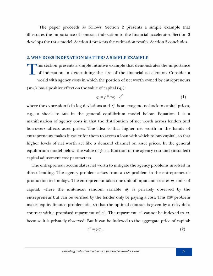
his section presents a simple intuitive example that demonstrates the importance

of indexation in determining the size of the financial accelerator. Consider a

world with agency costs in which the portion of net worth owned by entrepreneurs

( )tnw has a positive effect on the value of capital ( tq ):

* dt t tq p nw (1)

where the expression is in log deviations and dt is an exogenous shock to capital prices,

e.g., a shock to MEI in the general equilibrium model below. Equation 1 is a

manifestation of agency costs in that the distribution of net worth across lenders and

borrowers affects asset prices. The idea is that higher net worth in the hands of

entrepreneurs makes it easier for them to access a loan with which to buy capital, so that

higher levels of net worth act like a demand channel on asset prices. In the general

equilibrium model below, the value of p is a function of the agency cost and (installed)

capital adjustment cost parameters.

The entrepreneur accumulates net worth to mitigate the agency problems involved in

direct lending. The agency problem arises from a CSV problem in the entrepreneur’s

production technology. The entrepreneur takes one unit of input and creates t units of

capital, where the unit-mean random variable t is privately observed by the

entrepreneur but can be verified by the lender only by paying a cost. This CSV problem

makes equity finance problematic, so that the optimal contract is given by a risky debt

contract with a promised repayment of ptr . The repayment p

tr cannot be indexed to t

because it is privately observed. But it can be indexed to the aggregate price of capital:

pt tr q . (2)

T


This form of indexation is similar to indexing to the rate of return on capital in the

general equilibrium model developed below.

Entrepreneurial net worth accumulates with the profit flow from the investment

project, but decays via consumption of entrepreneurs (which is a constant fraction of net

worth). Log-linearized this evolution is given by:

1 p p nt t t t t tnw q r nw r (3)

where 1 denotes leverage (the ratio of project size to net worth) and nt is an

exogenous shock to net worth. Using the indexation assumption (2), we can express (3)

as

1[ ( 1)] nt t t tnw q nw (4)

Note that since κ > 1, the slope of the net worth equation is decreasing in the level of

indexation.

Equations 1 and 4 are a simultaneous system in net worth and the price of capital.

We can solve for the two endogenous variables as a function of the pre-determined and

exogenous variables:

1 [ ( 1)]

1 [ ( 1)]

n dt t t

t

nwnw

p

(5)

1( )

1 [ ( 1)]

n dt t t

t

p nwq

p

(6)

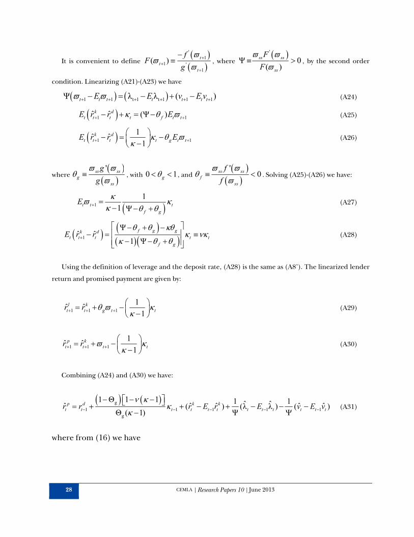
The inverse of the denominator in Equations 5-6 is the familiar multiplier arising from

two endogenous variables with positive feedback. This then implies that exogenous

shocks are multiplied or financially accelerated, and that the degree of this multiplication

depends upon the level of indexation. The effect of indexation on the financial

multiplier is highly nonlinear. Figure 1 plots the multiplier for κ = 2, and p = 0.45, both

of these values roughly correspond to the general equilibrium analysis below. Note that

moving from χ = 0 to χ = 1, has an enormous effect on the multiplier. But there are sharp

diminishing returns so the multiplier is little changed as we move from χ = 1 to χ = 2.

This suggests, and we confirm below, that the data can distinguish χ = 0 from, say, χ = 1,


but that indexation values in excess of unity will have similar business cycle

characteristics and thus be difficult to identify.

Consider three special cases of indexation: 0 , 1 , and 1 . The first is

the implicit assumption in BGG; the second implies complete indexation; the third

eliminates the financial accelerator altogether. In these cases, net worth and asset prices

are given by:

Indexation Net worth Capital price

Multiplier

(p=0.45, κ =2)

0 1

1

n dt t tnw

p

1( )

1

n dt t tp nw

p

10

1 1

1

n dt t tnw

p

1( )

1

n dt t tp nw

p

1.82

1

1 nt tnw 1( ) n d

t t tp nw 1

For both 0 and 1 , exogenous shocks to asset prices and net worth have

multiple effects on the equilibrium levels of net worth and capital prices. Since > 1,

this effect is much larger under BGG’s assumption of no indexation (1 1

)1 1

p p

.

Further, under the BGG assumption, exogenous shocks to asset prices ( dt ) have an

added effect as they are weighted by leverage. But for all levels of indexation, there are

always agency cost effects in that the price of capital is affected by the level of

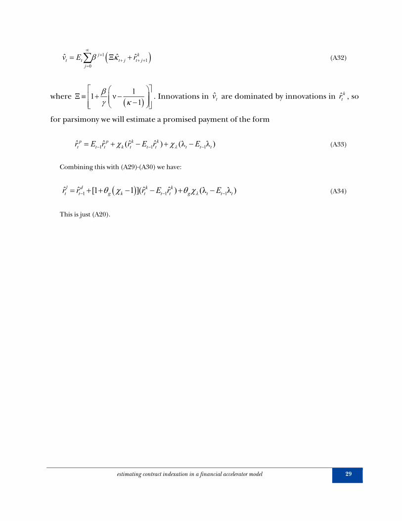
entrepreneurial net worth. The financial multiplier effects are traced out in Figure 2: an

exogenous shock to asset prices has a much larger effect on both net worth and asset

prices in the BGG framework. Finally, since 2 the financial accelerator largely

disappears when 2.

Before proceeding, it is helpful to emphasize the two parameters that are crucial in

our simple example as they will be manifested below in the richer general equilibrium


environment. Our reduced form parameter p in Equation 1 is the agency cost

parameter. In a Modigliani-Miller world we would have p = 0, as the distribution of net

worth would have no effect on asset prices or real activity. Second, the indexation

parameter χ determines the size of the financial accelerator, i.e., how do unexpected

movements in asset prices feed in to net worth? These are two related but logically

distinct ideas. That is, one can imagine a world with agency costs (p > 0), but with very

modest accelerator effects ( 1 . ). To anticipate our empirical results, this is the

parameter set that wins the model horse race. That is, the data is consistent with an

agency cost model but with trivial accelerator effects. In such an environment, financial

shocks (e.g., shocks to net worth) will affect real activity, but other real shocks (e.g., MEI

shocks) will not be accelerated.

3. THE MODEL

he benchmark model follows the JPT framework closely. The model of agency costs

comes from BGG with the addition of exogenous contract indexation. The BGG loan

contract is between lenders and entrepreneurs, so we focus on these two agents

first before turning to the familiar framework of JPT.

LENDERS

The representative lender accepts deposits from households (promising a sure real

return dtR ) and provides loans to the continuum of entrepreneurs. These loans are

intertemporal, with the loans made at the end of time t being paid back in time t+1. The

realized gross real return on these loans is denoted by 1LtR . Each individual loan is

subject to idiosyncratic and aggregate risk, but since the lender holds an entire portfolio

of loans, only the aggregate risk remains. The lender has no other source of funds, so

the level of loans will equal the level of deposits. Hence, real dividends are given by

1 1( ) L dt t t t tDiv R D R D . The intermediary seeks to maximize its equity value which is

given by:

T


t j

1 t

Λ

Λ

j

Lt t t j

j

Q E Div (7)

where Λ t is the marginal utility of real income for the representative household that

owns the lender.

The FOC of the lender’s problem is:

t 11

t

Λ0

Λ

L d

t t tE R R (8)

The first-order condition shows that in expectation, the lender makes zero profits,

but ex post profits and losses can occur.2 We assume that losses are covered by

households as negative dividends. This is similar to the standard assumption in the

dynamic new-Keynesian (DNK) model, e.g., Woodford (2003). That is, the sticky price

firms are owned by the household and pay out profits to the household. These profits

are typically always positive (for small shocks) because of the steady state mark-up over

marginal cost. Similarly, one could introduce a steady-state wedge (e.g., monopolistic

competition among lenders) in the lender’s problem so that dividends are always

positive. But this assumption would have no effect on the model’s dynamics so we

dispense from it for simplicity.

ENTREPRENEURS AND THE LOAN CONTRACT

Entrepreneurs are the sole accumulators of physical capital. At the beginning of period

t, the entrepreneurs sell all of their accumulated capital to capital agencies at beginning-

of-period capital price begtQ . At the end of the period, the entrepreneurs purchase the

entire capital stock tK , including any net additions to the stock, at end-of-period price

tQ . This re-purchase of capital is financed with entrepreneurial net worth ( tNW ) and

external financing from a lender. The external finance takes the form of a one period

loan contract. The gross return to holding capital from time-t to time t+1 is given by:

2 In contrast, BGG assume that bank profits are always zero ex post so that the lender’s return in pre-determined. This is not a feature of the optimal contract. See Carlstrom et al. (2013) for details.


11

begk tt

t

QR

Q. (9)

Below we show that 1 1 1 1 1 1 11 ( ) 1 begt t t t t t tQ Q u a u Q , the latter

term coinciding with the expression in BGG. Variations in 1ktR are the source of

aggregate risk in the loan contract. The external financing is subject to a costly-state-

verification (CSV) problem because of idiosyncratic risk. In particular, one unit of capital

purchased at time-t is transformed into 1 t units of capital in time t+1, where 1 t is an

idiosyncratic random variable with density and cumulative distribution Φ .

The realization of 1 t is directly observed by the entrepreneur, but the lender can

observe the realization only if a monitoring cost is paid, a cost that is fraction mc of the

project outcome. Assuming that the entrepreneur and lender are risk-neutral,

Townsend (1979) demonstrates that the optimal contract between entrepreneur and

intermediary is risky debt in which monitoring only occurs if the promised payoff is not

forthcoming. Payoff does not occur for sufficiently low values of the idiosyncratic shock,

1 1 t t . Let 1ptR denote the promised gross rate-of-return so that 1

ptR is defined by

1 1 1( ) p kt t t t t t t tR Q K NW R Q K . (10)

We find it convenient to express this in terms of the leverage ratio

t tt

t

Q K

NW so that

Equation 10 becomes

1 1 1 1

p k tt t t

t

R R (11)

With 1( ) tf and 1 tg denoting the entrepreneur’s share and lender’s share of the

project outcome, respectively, the lender’s ex post realized t+1 return on the loan

contract is defined as:

1 1

1 1 1 1

kt t t tL k t

t t tt t t t

R g Q KR R g

Q K NW (12)

where


[1 Φ ]

f d (13)

0

1 Φ (1 )

mcg d (14)

Recall that the lender’s stochastic discount factor comes from the household, and the

lender’s return is linked to the return on deposits via 8:

1 t 1 t 1Λ Λ L dt t t tE R R E (15)

As for the entrepreneur, Carlstrom, Fuerst and Paustian (2013) show that the

entrepreneur’s value function is linear with a time-varying coefficient we denote by tV ,

where tV satisfies:

1 1 1(1 ) kt t t t t tV EV R f (16)

Using this valuation and expression 15, the end-of-time-t contracting problem is thus

given by:

1, 1 1 1( ) t t

kt t t t tmax EV R f (17)

subject to

1 t 1 1 t 1Λ Λ1

k dtt t t t t

t

E R g R E (18)

An important observation is that the choice of 1 t can be made contingent on public

information available in time t+1. Indexation of this type is optimal. After some re-

arrangement, the contract optimization conditions include:

'1 1' '

1 1 t 1 1't 1 1

ΛΛ

t t tt t t

t t

EV fV f g

E g (19)

'

1 11 1 1 t 1 1 1'

t 1 1

( 1) ΛΛ

t t tk kt t t t t t t t

t t

EV fEV R f E R g

E g (20)

t 1 1 1 t 1Λ Λ1

k dtt t t t t

t

E R g R E (21)


A key result is given by (19). The optimal monitoring cut-off 1 t is independent o K

K innovations in 1ktR . The second-order condition implies that the ratio

'1

'1

t

t

f

g is

increasing in 1 t . Hence, another implication of the privately optimal contract is that

1 t (and thus the optimal repayment rate 1ptR ) is an increasing function of (innovations

in) the marginal utility of wealth t 1Λ , and a decreasing function of (innovations in) the

entrepreneur’s valuation 1tV .

The monitoring cut-off implies the behavior of the repayment rate (see 11). In log

deviations, Carlstrom, Fuerst, and Paustian (2013) show that the repayment rate under

the optimal contract is given by:

g

1 1 1 1 1g

1 Θ 1 1 1 1ˆ ˆˆ ( ) (λ λ ) ( )Θ ( 1

ˆ ˆΨ

ˆ)

ˆ

p d k kt t t t t t t t t t t tr r r E r E v E v (22)

11

0

Ξ ˆˆ ˆ

j kt t t j t j

j

v E r (23)

where the hatted lower case letters denote log deviations, and the positive constants Ξ

and are defined in the Appendix. Innovations in ˆtv will be driven by innovations in

ˆktr . Hence, for parsimony we will estimate an indexation rule of the form:

1 1 1ˆ ˆΩ (λ λ )ˆ( ) p k kt t k t t t t t tr r E r E (24)

where 1Ω t are the pre-determined variables that affect the repayment rate, e.g., 1 t . As

noted in the example sketched in Section 2, different indexation values will have

dramatic effects on the financial accelerator. The original BGG model assumes that the

lender’s return was pre-determined. From Equations 11-12, this implies that 0 and

0 k , where k is modestly negative ( 0.01 k , in our benchmark calibration).

Entrepreneurs have linear preferences and discount the future at rate β. Given

the high return to internal funds, they will postpone consumption indefinitely. To limit

net worth accumulation and ensure that there is a need for external finance in the long

run, we assume that fraction (1-γ) of the entrepreneurs die each period. Their


accumulated assets are sold and the proceeds transferred to households as consumption.

Given the exogenous death rate, aggregate net worth accumulation is described by

t 1 1 ,NW γ ( ) kt t t t nw tNW R f (25)

where ,nw t is an exogenous disturbance to the distribution of net worth. We assume it

follows the stochastic process

, , 1 ,log , nw t nw nw t nw tlog (26)

where , nw t is i.i.d. N(0, 2 nw ). Equation 25 implies that tNW is determined by the

realization of ktR and the response of t to these realizations. tNW then enters the

contracting problem in time t so that the realization of ktR is propagated forward.

As in Christiano, Motto, and Rostagno (2010), and Gilchrist, Ortiz and Zakrajšek

(2009), we also consider time variation in the variance of the idiosyncratic shock t . The

variance of t is denoted by t and follows the exogenous stochastic process given by

1 ,log , t t tlog (27)

Shocks to this variance will alter the risk premium in the model.

FINAL GOOD PRODUCERS

Perfectly competitive firms produce the final consumption good Yt combining a

continuum of intermediate goods according to the CES technology:

p ,t

p ,t

1 λ11/(1 λ )

0

( )

t tY Y i di (28)

The elasticity ,p t follows the exogenous stochastic process

, , 1 , , 1 1 log log , p t p p p p t p t p p tlog (29)

where εp,t is i.i.d. N(0, 2p ). Fluctuations in this elasticity are price markup shocks. Profit

maximization and the zero profit condition imply that the price of the final good, Pt, is

the familiar CES aggregate of the prices of the intermediate goods.


INTERMEDIATE GOODS PRODUCERS

A monopolist produces the intermediate good i according to the production function

α

1 1 1 αtmax ( ) ( ) Υ ;0, t t t t tY i A K i L i A F (30)

where Kt(i) and Lt(i) denote the amounts of capital and labor employed by firm i. F is a

fixed cost of production, chosen so that profits are zero in steady state. The variable tA is

the exogenous non-stationary level of TFP progress. Its growth rate (zt ≡ ΔlnAt ) is given by

1 ,1 , t z z z t z tz z (31)

where εz,t is i.i.d.N(0, 2 z ). The other non-stationary process t is linked to the investment

sector and is discussed below.

Every period a fraction p of intermediate firms cannot choose its price optimally,

but resets it according to the indexation rule

11 1 , p p

t t tP i P i (32)

where πt ≡ Pt/Pt-1 is gross inflation and π is its steady state. The remaining fraction of firms

chooses its price Pt (i) optimally, by maximizing the present discounted value of future

profits

11

0 1

/ ( )

/

p p

s ss t s t s

t p t t k t s t s t s t s t s t ss kt t

PE P i Y i W L i P K i

P (33)

where the demand function comes from the final goods producers, /t tP is the

marginal utility of nominal income for the representative household, and Wt is the

nominal wage.

EMPLOYMENT AGENCIES

Firms are owned by a continuum of households, indexed by 0,1j . Each household is

a monopolistic supplier of specialized labor, Lt(j), as in Erceg et al. (2000). A large

number of competitive employment agencies combine this specialized labor into a

homogenous labor input sold to intermediate firms, according to


,

,

111/(1 )

0

( )

w t

w t

t tL L j dj (34)

As in the case of the final good, the desired markup of wages over the household’s

marginal rate of substitution, , ,w t follows the exogenous stochastic process

, , 1 , , 1log 1 log , w t w w w w t w t w w tlog (35)

where ,w t is i.i.d. N (0, 2w). This is the wage markup shock. Profit maximization by the

perfectly competitive employment agencies implies that the wage paid by intermediate

firms for their homogenous labor input is

,

,

11/

0

( )

w t

w t

t tW W j dj (36)

CAPITAL AGENCIES

The capital stock is managed by a collection of perfectly competitive capital agencies.

These firms are owned by households and discount cash flows with Λ t, the marginal

utility of real income for the representative household. At the beginning of period t,

these agencies purchase the capital stock 1tK from the entrepreneurs at beginning-of-

period price begtQ . The agencies produce capital services by varying the utilization rate ut

which transforms physical capital into effective capital according to

1. tt t KK u (37)

Effective capital is then rented to firms at the real rental rate . t The cost of capital

utilization is ( )ta u per unit of physical capital. The capital agency then re-sells the capital

to entrepreneurs at the end of the period at price tQ . The profit flow is thus given by:

1 1 11 ( ) begt t tt t t t tQ u a u KQK K (38)

Profit maximization implies

1 ( ) begt t t t tQ Q u a u (39)

'( ) t ta u (40)


In steady state, u = 1, a(1) = 0 and ≡ a'' (1)/a'(1). Hence, in the neighbourhood of

the steady state

1 begt t tQ Q (41)

which is consistent with BGG’s definition of the intertemporal return to holding capital

1

1

t tk

tt

QR

Q.

NEW CAPITAL PRODUCERS

New capital is produced according to the production technology that takes tI

investment goods and transforms them into -1

1-

tt t

t

IS II

new capital goods. The

time-t profit flow is thus given by

-1

1- -

Itt t t t t

t

IQ S I P I

I (42)

where ItP is the relative price of the investment good. The function S captures the

presence of adjustment costs in investment, as in Christiano et al. (2005). The function

has the following convenient steady state properties: S = S' = 0 and S'' >0. These firms are

owned by households and discount future cash flows with Λ t, the marginal utility of real

income for the representative household. JPT refer to the investment shock μt as a shock

to the marginal efficiency of investment (MEI) as it alters the transformation between

investment and installed capital. JPT conclude that this shock is the primary driver of

output and investment at business cycle frequencies. The investment shock follows the

stochastic process

1 , , t t tlog log (43)

where , t is i.i.d. N 20, .


INVESTMENT PRODUCERS

A competitive sector of firms produces investment goods using a linear technology that

transforms one consumption good into t investment goods. The exogenous level of

productivity t is non-stationary with a growth rate ( t ≡ Δlog tΥ ) given by

1 ,1 t t t . (44)

The constant returns production function implies that the price of investment goods

(in consumption units) is equal to t

1

.

HOUSEHOLDS

Each household maximizes the utility function

1

10

( ) ln ,

1

s t s

t t s t s t ss

L jE b C hC (45)

where Ct is consumption, h is the degree of habit formation and bt is a shock to the

discount factor. This intertemporal preference shock follows the stochastic process

1 , , t b t b tlogb logb (46)

where ,b t is i.i.d. N(0, 2b ). Since technological progress is nonstationary, utility is

logarithmic to ensure the existence of a balanced growth path. The existence of state

contingent securities ensures that household consumption is the same across all

households. The household’s flow budget constraint is

1 1

1 1 , t dt t t

t t t t t t tt t t

W jB R BC T D L j D R profits

P P P (47)

where tD denotes real deposit at the lender, Tt is lump-sum taxes, and Bt is holdings of

nominal government bonds that pay gross nominal rate Rt . The term tprofits denotes

the combined profit flow of all the firms owned by the representative agent including

lenders, intermediate goods producers, capital agencies, and new capital producers.

Every period a fraction ξw of households cannot freely set its wage, but follows the

indexation rule


1 11 11 1 ( )( ) ( ) ,

t t z

w wz

t t tW j eW j e (48)

The remaining fraction of households chooses instead an optimal wage Wt(j) by

maximizing

1

0

( ) Λ( )

1

s s t S t s

t w t s t t ss t s

L jE b W j L j

P (49)

subject to the labor demand function coming from the firm.

THE GOVERNMENT

A monetary policy authority sets the nominal interest rate following a feedback rule of

the form

xπ

1

1 1,* * *

1

X / ,

X / X

RdxR

t t t t t tmp t

t t t

R R X X

R R X (50)

where R is the steady state of the gross nominal interest rate. The interest rates respond

to deviations of inflation from its steady state, as well as to the level and the growth rate

of the GDP gap ( tX / *tX ). The monetary policy rule is also perturbed by a monetary

policy shock, ,mp t , which evolves according to

, , 1 ,log , mp t mp mp t mp tlog (51)

where , mp t is i.i.d. N 2(0, )mp . Public spending is determined exogenously as a time-

varying fraction of output.

1

1- ,

t tt

G Yg

(52)

where the government spending shock gt follows the stochastic process

1 ,log 1 log , t g g t g tg g log g (53)

with 2g,t g~ . . . 0, i i d N . The spending is financed with lump sum taxes.

MARKET CLEARING

The aggregate resource constraints are given by:


1

t

t

t t t tt

IC G a u Y (54)

-1

0 -1

1- 1- 1- ,

tvt

t tmc t tt

K KI

f d S IIò (55)

This completes the description of the model. We now turn to the estimation of the

linearized model.

4. ESTIMATION

he linearized version of the model equations are collected in the appendix. The

three fundamental agency cost parameters are the steady state idiosyncratic

variance ( ) ss , the entrepreneurial survival rate (γ), and the monitoring cost

fraction (mc ). In contrast to DeGraeve (2008), we follow Christiano et al. (2010), and

calibrate these parameters to be consistent with long run aspects of US financial data. We

follow this calibration approach because these parameters are pinned down by long run

or steady state properties of the model, not the business cycle dynamics that the Bayesian

estimation is trying to match. In any event, these three parameters are calibrated to

match the steady state levels of the risk premium ( )p dR R , leverage ratio ( ), and

default rate (Φ( )) ss . In particular, they are chosen to deliver a 200 bp annual risk

premium (BAA-Treasury spread), a leverage ratio of = 1.95, and a quarterly default

rate of 0.03/4. These imply an entrepreneurial survival rate of γ = 0.98, a standard

deviation of ss = 0.28, and a monitoring cost of mc = 0.12. A key expression in the log-

linearized model is the reduced-form relationship between the risk premium and

leverage:

1ˆˆ ˆ ˆ ˆ ˆ k d

t t t t t t tE r r q k n (56)

T


(See the Appendix for details.) The value of ν implied by the previous calibration is ν =

0.041. This is thus imposed in the estimation of the financial models.3 For JPT we have ν =

0. Steady state relationships also imply that we calibrate δ = 0.025, and (1-1/g) = 0.22. The

remaining parameters are estimated using familiar Bayesian techniques as in JPT. For the

non-financial parameters of the model we use the same priors as in JPT.

We treat as observables the growth rates of real GDP, consumption, investment, the

real wage, and the relative price of investment. The other observables include

employment, inflation, the nominal rate, leverage, and the risk premium. Employment

is measured as the log of per capita hours. Inflation is the consumption deflator, and the

nominal rate is the federal funds rate. The series for leverage comes from Gilchrist,

Ortiz and Zakrajsek (2009). The risk premium is the spread between the BAA and ten

year Treasury. The time period for the estimation is 1954:3-2009:1. We choose the end of

the sample period to avoid the observed zero bound on the nominal rate.

We estimate four versions of the model. Along with all the exogenous shocks outlined

in the paper, we also include autocorrelated measurement error between the model’s

risk premium and the observed risk premium. Autocorrelated measurement error is also

included for leverage. The first model we label JPT as it corresponds to the model

without agency costs (ν = 0). Note that to match the observed financial variables, the JPT

model will assign all risk premium and leverage variation to autocorrelated

measurement error. The remaining three models have operative agency costs (ν =

0.041). Recall that the optimal contract has the form given in Equation 24. Our three

estimates consider variations on this basic form. In the model labeled BGG we impose the

level of indexation implicitly assumed by BGG: 0.01 k , 0 . For the model labeled

Rk-indexation, we set 0 and estimate the value of k . For the model labeled Rk & λ-

indexation, we estimate both indexation parameters. We use diffuse priors on the

3 As a form of sensitivity analysis, we also estimated in the financial models. We found that the

estimation is quite sensitive to priors, again suggesting that it is not well identified by business cycle

dynamics.


indexation parameters with a uniform distribution centered at 0 and with a standard

deviation of 2.

The agency cost models also include two financial shocks: i) time-varying movements

in idiosyncratic risk, and ii) exogenous redistributions of net worth. Both of these shocks

are irrelevant in the JPT model in which lending is not subject to the CSV problem. We

posit priors for the standard deviation and autocorrelation of these financial shocks in a

manner symmetric with the non-financial exogenous processes in JPT.

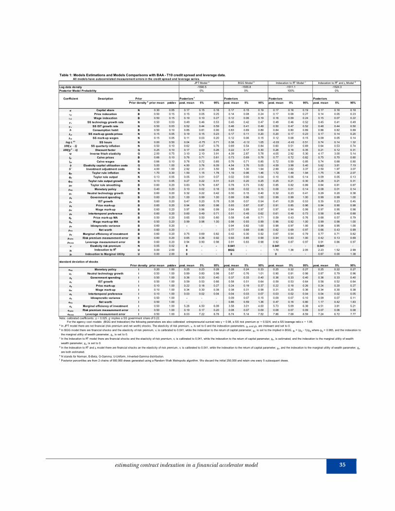
The estimation results are summarized in Table 1. The BGG, Rk-indexation, and Rk &

λ-indexation agency cost models dominate the JPT model as the JPT model cannot

capture the forecastability of leverage and the risk premium that is in the data.

Comparing BGG and Rk-indexation, the data rejects the BGG level of indexation

preferring a level of contract indexation that is economically significant: k = 1.70 with a

90% confidence interval between 1.36 and 2.05. Results are on a similar range in the

case of the Rk & λ-indexation estimation with k = 2.23 with a 90% confidence interval

between 1.52 and 2.99. As suggested by the example in Section 2, this level of indexation

will imply significantly different responses to shocks compared to the BGG assumption.

We will see this manifested in the IRF below. The estimated level of indexation to the

marginal utility of wealth is = 0.67 with a 90% confidence interval between 0 and

1.38. The combination of the two indexation parameters under the Rk & λ-indexation

specification generates dynamics that are similar to those of the Rk-indexation sp

ecification alone.

Two other differences in parameter estimates are worth some comment. First, the

BGG model estimates a significantly smaller size for investment adjustment costs ( "S ) in

the table: "S = 1.68 for BGG, but 2.99 for Rk-indexation, 2.50 for Rk & λ-indexation, and

2.92 for JPT. The level of adjustment costs has two contrasting effects. First, lower

adjustment costs will increase the response of investment to aggregate shocks. Second,

lower adjustment costs imply smaller movements in the price of installed capital (Qt)

and thus smaller financial accelerator effects in the BGG model.


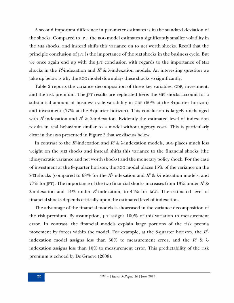
A second important difference in parameter estimates is in the standard deviation of

the shocks. Compared to JPT, the BGG model estimates a significantly smaller volatility in

the MEI shocks, and instead shifts this variance on to net worth shocks. Recall that the

principle conclusion of JPT is the importance of the MEI shocks in the business cycle. But

we once again end up with the JPT conclusion with regards to the importance of MEI

shocks in the Rk-indexation and Rk & λ-indexation models. An interesting question we

take up below is why the BGG model downplays these shocks so significantly.

Table 2 reports the variance decomposition of three key variables: GDP, investment,

and the risk premium. The JPT results are replicated here: the MEI shocks account for a

substantial amount of business cycle variability in GDP (60% at the 8-quarter horizon)

and investment (77% at the 8-quarter horizon). This conclusion is largely unchanged

with Rk-indexation and Rk & λ-indexation. Evidently the estimated level of indexation

results in real behaviour similar to a model without agency costs. This is particularly

clear in the IRFs presented in Figure 3 that we discuss below.

In contrast to the Rk-indexation and Rk & λ-indexation models, BGG places much less

weight on the MEI shocks and instead shifts this variance to the financial shocks (the

idiosyncratic variance and net worth shocks) and the monetary policy shock. For the case

of investment at the 8-quarter horizon, the BGG model places 15% of the variance on the

MEI shocks (compared to 68% for the Rk-indexation and Rk & λ-indexation models, and

77% for JPT). The importance of the two financial shocks increases from 13% under Rk &

λ-indexation and 14% under Rk-indexation, to 44% for BGG. The estimated level of

financial shocks depends critically upon the estimated level of indexation.

The advantage of the financial models is showcased in the variance decomposition of

the risk premium. By assumption, JPT assigns 100% of this variation to measurement

error. In contrast, the financial models explain large portions of the risk premia

movement by forces within the model. For example, at the 8-quarter horizon, the Rk-

indexation model assigns less than 50% to measurement error, and the Rk & λ-

indexation assigns less than 10% to measurement error. This predictability of the risk

premium is echoed by De Graeve (2008).


Why does the BGG model downplay the MEI shocks and thus shift variance to the other

shocks? The answer is quite apparent from Figure 3a. The figure sets all parameter

values to those estimated in the Rk-indexation model, except for the levels of indexation

( k ≈ 0 for BGG and k = 2.23 and = 0.67 for the Rk & λ-indexation model), and the

level of agency cost effects (ν = 0 for JPT).4 A positive innovation in MEI leads to a fall in

the price of capital. Since the BGG contract is not indexed to the return to capital, the

shock leads to a sharp decline in entrepreneurial net worth, and thus a sharp increase in

the risk premium. This procyclical movement in the risk premium is in sharp contrast to

the data. Hence, the Bayesian estimation in the BGG model estimates only a small

amount of variability coming from the MEI shocks. Notice that in the Rk-indexation and

Rk & λ-indexation models net worth is almost unchanged in response to an MEI shock, so

that the impact effect on the risk premium is countercyclical. The main difference

among models is the behavior of the repayment that under credit contract indexation is

lowered in response to the drop in the return on capital, while in BGG it remains

unchanged. The Rk-indexation and Rk & λ-indexation models are thus consistent with

MEI shocks driving the cycle, and the risk premium being countercyclical. The similarity

of the Rk-indexation and JPT model is also apparent: the two IRFs to an MEI shock largely

lie on top of one another.

Since the BGG model downplays the importance of MEI shocks, and shifts this variance

to other shocks. Figures 3b-3c plot the IRFs to the two financial shocks. The good news

with the two financial shocks is that the spread is now countercyclical. But the difficulty

with the financial shocks is that they result in countercyclical consumption. This is the

familiar co-movement puzzle that arises when a positive shock in one sector (e.g., higher

net worth mitigates agency costs in capital accumulation) leads to a downward

production movement in the other sector. However, this comovement problem does not

arise with risk premium shocks in the Rk-indexation and Rk & λ-indexation models. As an

4Alternatively we could have considered the IRFs for each model at each model’s parameter estimates. These IRFs are similar to those reported here, but we find Figure 3 more intuitive as it is holding all other parameters fixed except for the degree of indexation and the presence of agency costs.


aside, note that a shock to net worth has a larger effect on net worth and capital prices in

the BGG model. This is just a manifestation of the multiplier intuition outlined in Section

2.

Figure 3d plots the IRF to a monetary shock. In the case of BGG, the IRFs exhibit

plausible comovement and countercyclical spreads. The BGG estimation does not put

more weight on these policy shocks because the funds rate is an observable, and thus

limits possible interest rate variability. In contrast, it is quite clear why the Indexation

model puts so little weight on monetary policy shocks. In the case of Indexation, the

spread is procyclical, a clear counterfactual prediction.

As a form of sensitivity analysis, Table 3 presents the estimation results for i.i.d.

measurement error in the financial variables. The Rk & λ-indexation now wins the model

horse race, with JPT coming in significantly worse than the three financial models. The

degree of Rk-indexation is much larger than the case with autocorrelated measurement

error. Further the level of indexation to the marginal utility of wealth is estimated to be

significantly positive, in line with the theory outlined above.

5. CONCLUSION

his paper began as an empirical investigation of the importance of agency costs

and contract indexation in the business cycle. To reiterate, our principle results

include the following. First, the financial models appear to be an improvement

over the financial-frictionless JPT. Second, Rk-indexation appears to be an important

characteristic of the data. Third, the importance of financial shocks (net worth and

idiosyncratic variance) in explaining the business cycle is significantly affected by the

estimated degree of Rk-indexation. In short, we find evidence for the importance of

financial shocks in the business cycle. But the evidence also suggests that the effect of

non-financial shocks on real activity is unaffected by the inclusion of financial forces in

the model. That is, the results suggest the importance of financial shocks, but not the

existence of a financial accelerator. This analysis thus implies that Bayesian estimation of

T


financial models should include estimates of contract indexation. Empirical analyses

that impose zero contract indexation likely distort both the source of business cycle

shocks and their transmission mechanism.


APPENDIX

1. Linearized System of Equations:

(1 )ˆ ˆˆ t t t

y Fy k L

y (A1)

ˆˆˆ ˆ t t t tw L k (A2)

ˆ (1 )ˆ ˆ t t ts w (A3)

1 1 ,

ˆˆ ˆ ˆ ˆ1 1

1 1 1

p pp

t t t t t p tp p p p

E s (A4)

2 2

1 1ˆ ˆ ˆ ˆ

z z z

z z z z z zt t t t t

h e e h heE c c c

e h e h e h e h e h e h

1( ) ( )

ˆ ˆˆ

z z zz z

z z z z z

bzt t t

e h h e heh e hez b

e h e h e h e h e h (A5)

1 1 1 1ˆ ˆˆ ˆˆ(

1ˆ )

t t t t t t tR E z (A6)

ˆ ˆ t tu (A7)

1 1 1 1ˆ ˆ ˆˆ ˆ

1

k

t t t t t t t t tE r E E z E (A8)

2( ) "1

ˆ ˆ ˆ1

ˆ1

ˆ ˆ

z

t t t t t tq e S i i z

2( ) "1 1 1

ˆ ˆ ˆˆ1

1

z

t t t t te S E i i z (A9)

1

1ˆ 1

ˆˆ ˆ

tt t t tk u k z (A10)

( ) ( )1 ˆˆ ˆˆ

11 1 1 ( )

1

z zt t t t t tk e k z e i (A11)

1 1 , 1ˆ ˆ

1 11

1ˆ

1 1ˆ ˆ

1

w w w

t t t t w t tw w

w w E w g


1 1 1ˆˆ ˆ ˆ1

1 1ˆ

1

1 1 1

w w w z

t t t t t tE z z

,

1

1ˆˆ

1

wt w t (A12)

,ˆ ˆˆ(ˆ ˆ ) w t t t t tg w L b (A13)

* * *1 1 1 ,1 )ˆ ˆ ˆ(ˆ ˆ ˆ ˆ ˆ ˆ ˆ

t R t R t x t t dx t t t t mp tR R x x x x x x (A14)

ˆ ˆ ˆ

t t t

kx y u

y (A15)

1 ˆˆ ˆ ˆ ˆ1

t t t t t

c i ky g c i u

g g y y y (A16)

1ˆˆ d

t t t tr R E (A17)

( ) ( )1(1 ) ˆˆ 1 ˆ1 (ˆ )

z zkt t t tr e q e q (A18)

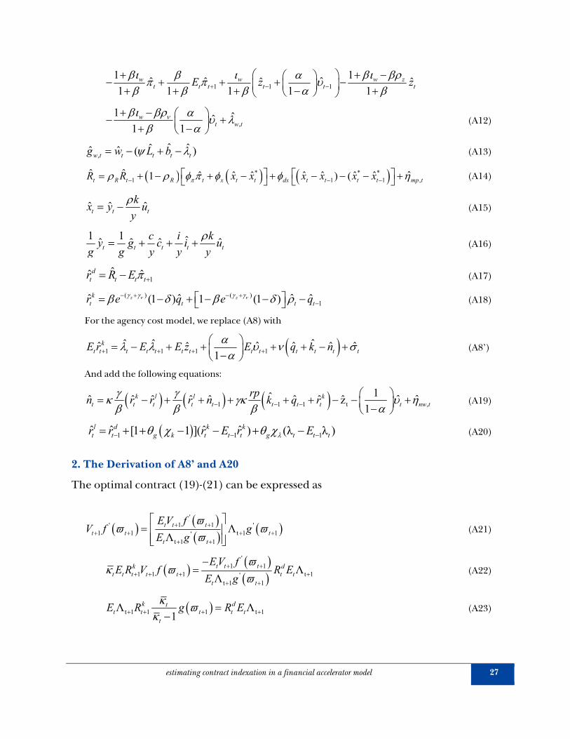
For the agency cost model, we replace (A8) with

1 1 1 1ˆˆ ˆ ˆˆ ˆ ˆ ˆ

1ˆ

k

t t t t t t t t t t t t tE r E E z E q k n (A8’)

And add the following equations:

1 1 1 t ,

1zˆ ˆ ˆˆ ˆ ˆ ˆ ˆ ˆ

1ˆ ˆ

k l l k

t t t t t t t t t nw t

rpn r r r n k q r (A19)

1 1 1[1 1 ]( ) (ˆ ˆ λˆ λ )ˆ l d k kt t g k t t t g t t tr r r E r E (A20)

2. The Derivation of A8’ and A20

The optimal contract (19)-(21) can be expressed as

'1 1' '

1 1 t 1 1't 1 1

ΛΛ

t t tt t t

t t

EV fV f g

E g (A21)

'1 1

1 1 1 t 1't 1 1

ΛΛ

t t tk d

t t t t t t tt t

EV fE R V f R E

E g (A22)

t 1 1 1 t 1Λ Λ1

k dtt t t t t

t

E R g R E (A23)


It is convenient to define

'1

1 '1

( )

t

tt

fF

g, where

'

Ψ 0( )

ss ss

ss

F

F, by the second order

condition. Linearizing (A21)-(A23) we have

1 1 t 1 t 1 1 1 Ψ λ λ ( ) t t t t t t tE E v E v (A24)

1 1ˆ ˆ (Ψ ) k dt t t t f t tE r r E (A25)

1 1

1

1ˆ ˆ

k dt t t t g t tE r r E (A26)

where

'

ss ssg

ss

g

g, with 0 1 g , and

'0

ss ss

fss

f

f. Solving (A25)-(A26) we have:

1

1

1 Ψ

t t t

f g

E (A27)

1

Ψ

1ˆ

Ψˆ

f g gk dt t t t t

f g

E r r (A28)

Using the definition of leverage and the deposit rate, (A28) is the same as (A8’). The linearized lender

return and promised payment are given by:

1 1 1

1

1ˆ ˆ

l kt t g t tr r (A29)

1 1 1

1

1ˆ ˆ

p kt t t tr r (A30)

Combining (A24) and (A30) we have:

g

1 1 1 1 1g

1 Θ 1 1 1 1ˆ ˆˆ ( ) (λ λ ) ( )Θ ( 1

ˆ ˆΨ

ˆ)

ˆ

p d k kt t t t t t t t t t t tr r r E r E v E v (A31)

where from (16) we have


11

0

Ξ ˆˆ ˆ

j kt t t j t j

j

v E r (A32)

where

1Ξ 1 ν

1

. Innovations in ˆtv are dominated by innovations in ˆktr , so

for parsimony we will estimate a promised payment of the form

1 1 1ˆ ˆ ˆ( ) (λ λˆ ) p p k kt t t k t t t t t tr E r r E r E (A33)

Combining this with (A29)-(A30) we have:

1 1 1[1 1 ]( ) (ˆ ˆ λˆ λ )ˆ l d k kt t g k t t t g t t tr r r E r E (A34)

This is just (A20).


Figure 1 The Multiplier as a Function of Indexation.

Figure 2 A Shock to Asset Demand

(Asset price is blue line. Net worth evolution is red line.) Demand shock shifts up

asset price. The new equilibrium in (n,q) space depends upon the level of indexation.

Lower levels of indexation amplify these effects.

q

n

"=1"=0


Figure 3.a. Impulse Response Functions to a One Standard Deviation Marginal Efficiency of Investment Shock Keeping parameters constant to the Rk indexation model except Rk and lambda indexation parameters (χk and χλ)

_______ JPT ……........ BGG _ _ _ _ _ Indexation to Rk_ . _ . _ Indexation to Rk and λ

0

0.1

0.2

0.3

0.4

0.5

0.6

0.7

0.8

0.9

1

1 5 9 13 17

Output

‐0.05

0

0.05

0.1

0.15

0.2

0.25

0.3

0.35

0.4

1 5 9 13 17

Consumption

‐2

‐1

0

1

2

3

4

5

1 5 9 13 17

Investment

‐0.06

‐0.04

‐0.02

0

0.02

0.04

0.06

0.08

0.1

0.12

0.14

1 5 9 13 17

Inflation

0

0.02

0.04

0.06

0.08

0.1

0.12

0.14

0.16

0.18

0.2

1 5 9 13 17

Wages

‐0.2

‐0.1

0

0.1

0.2

0.3

0.4

0.5

0.6

1 5 9 13 17

Federal Funds

‐0.1

‐0.05

0

0.05

0.1

0.15

0.2

0.25

0.3

1 5 9 13 17

Spread

‐3

‐2.5

‐2

‐1.5

‐1

‐0.5

0

0.5

1

1 5 9 13 17

Net Worth

‐1.4

‐1.2

‐1

‐0.8

‐0.6

‐0.4

‐0.2

0

1 5 9 13 17

Price of Capital

‐1.4

‐1.2

‐1

‐0.8

‐0.6

‐0.4

‐0.2

0

0.2

0.4

1 5 9 13 17

Return on Capital (Rk)

‐2

‐1.5

‐1

‐0.5

0

0.5

1 5 9 13 17

Promised Repayment

‐0.6

‐0.4

‐0.2

0

0.2

0.4

0.6

1 5 9 13 17

Marginal Utility of Wealth (λ)


Figure 3.b. Impulse Response Functions to a One Standard Deviation Net Worth Shock Keeping parameters constant to the Rk indexation model except Rk and lambda indexation parameters (χk and χλ)

……........ BGG _ _ _ _ _ Indexation to Rk_ . _ . _ Indexation to Rk and λ

0

0.05

0.1

0.15

0.2

0.25

1 5 9 13 17

Output

‐0.2

‐0.15

‐0.1

‐0.05

0

0.05

1 5 9 13 17

Consumption

0

0.2

0.4

0.6

0.8

1

1.2

1.4

1.6

1.8

1 5 9 13 17

Investment

‐0.035

‐0.03

‐0.025

‐0.02

‐0.015

‐0.01

‐0.005

0

0.005

0.01

0.015

0.02

1 5 9 13 17

Inflation

‐0.01

0

0.01

0.02

0.03

0.04

0.05

0.06

0.07

0.08

0.09

1 5 9 13 17

Wages

0

0.02

0.04

0.06

0.08

0.1

0.12

0.14

0.16

1 5 9 13 17

Federal Funds

‐0.3

‐0.25

‐0.2

‐0.15

‐0.1

‐0.05

0

1 5 9 13 17

Spread

0

0.2

0.4

0.6

0.8

1

1.2

1.4

1.6

1.8

2

1 5 9 13 17

Net Worth

‐0.05

0

0.05

0.1

0.15

0.2

0.25

1 5 9 13 17

Price of Capital

‐0.05

0

0.05

0.1

0.15

0.2

0.25

1 5 9 13 17


‐0.05

0

0.05

0.1

0.15

0.2

0.25

0.3

1 5 9 13 17

Promised Repayment

‐0.1

0

0.1

0.2

0.3

0.4

0.5

0.6

1 5 9 13 17



Figure 3.c. Impulse Response Functions to a One Standard Deviation Idiosyncratic Variance Shock Keeping parameters constant to the Rk indexation model except Rk and lambda indexation parameters (χk and χλ)

……........ BGG _ _ _ _ _ Indexation to Rk_ . _ . _ Indexation to Rk and λ

‐0.35

‐0.3

‐0.25

‐0.2

‐0.15

‐0.1

‐0.05

0

1 5 9 13 17

Output

‐0.12

‐0.1

‐0.08

‐0.06

‐0.04

‐0.02

0

0.02

0.04

0.06

1 5 9 13 17

Consumption

‐2

‐1.8

‐1.6

‐1.4

‐1.2

‐1

‐0.8

‐0.6

‐0.4

‐0.2

0

1 5 9 13 17

Investment

‐0.35

‐0.3

‐0.25

‐0.2

‐0.15

‐0.1

‐0.05

0

1 5 9 13 17

Inflation

‐0.1

‐0.09

‐0.08

‐0.07

‐0.06

‐0.05

‐0.04

‐0.03

‐0.02

‐0.01

0

1 5 9 13 17

Wages

‐0.4

‐0.35

‐0.3

‐0.25

‐0.2

‐0.15

‐0.1

‐0.05

0

1 5 9 13 17

Federal Funds

0

0.05

0.1

0.15

0.2

0.25

0.3

0.35

0.4

0.45

0.5

1 5 9 13 17

Spread

‐1.5

‐1

‐0.5

0

0.5

1

1 5 9 13 17

Net Worth

‐0.7

‐0.6

‐0.5

‐0.4

‐0.3

‐0.2

‐0.1

0

0.1

1 5 9 13 17

Price of Capital

‐0.7

‐0.6

‐0.5

‐0.4

‐0.3

‐0.2

‐0.1

0

0.1

0.2

0.3

1 5 9 13 17


‐1

‐0.8

‐0.6

‐0.4

‐0.2

0

0.2

0.4

1 5 9 13 17

Promised Repayment

‐0.25

‐0.2

‐0.15

‐0.1

‐0.05

0

0.05

0.1

0.15

0.2

1 5 9 13 17



Figure 3.d. Impulse Response Functions to a One Standard Deviation Monetary Policy Shock Keeping parameters constant to the Rk indexation model except Rk and lambda indexation parameters (χk and χλ)

_______ JPT ……........ BGG _ _ _ _ _ Indexation to Rk_ . _ . _ Indexation to Rk and λ

‐0.45

‐0.4

‐0.35

‐0.3

‐0.25

‐0.2

‐0.15

‐0.1

‐0.05

0

1 5 9 13 17

Output

‐0.25

‐0.2

‐0.15

‐0.1

‐0.05

0

1 5 9 13 17

Consumption

‐1.6

‐1.4

‐1.2

‐1

‐0.8

‐0.6

‐0.4

‐0.2

0

0.2

0.4

1 5 9 13 17

Investment

‐0.25

‐0.2

‐0.15

‐0.1

‐0.05

0

1 5 9 13 17

Inflation

‐0.06

‐0.05

‐0.04

‐0.03

‐0.02

‐0.01

0

1 5 9 13 17

Wages

‐0.1

0

0.1

0.2

0.3

0.4

0.5

0.6

0.7

0.8

0.9

1 5 9 13 17

Federal Funds

‐0.1

‐0.05

0

0.05

0.1

0.15

1 5 9 13 17

Spread

‐2

‐1.5

‐1

‐0.5

0

0.5

1 5 9 13 17

Net Worth

‐1

‐0.9

‐0.8

‐0.7

‐0.6

‐0.5

‐0.4

‐0.3

‐0.2

‐0.1

0

0.1

1 5 9 13 17

Price of Capital

‐1

‐0.8

‐0.6

‐0.4

‐0.2

0

0.2

0.4

1 5 9 13 17


‐1.6

‐1.4

‐1.2

‐1

‐0.8

‐0.6

‐0.4

‐0.2

0

0.2

0.4

1 5 9 13 17

Promised Repayment

0

0.2

0.4

0.6

0.8

1

1.2

1 5 9 13 17



Table 1: Models Estimations and Models Comparisons with BAA - T10 credit spread and leverage data. All models have autocorrelated measurement errors in the credit spread and leverage series.

JPT Model a BGG Model b Indexation to Rk Model c Indexation to Rk and λ Model d

Log data density -1590.5 -1555.8 -1511.1 -1524.3Posterior Model Probability 0% 0% 100% 0%

Coefficient Description Prior Posteriors f Posteriors Posteriors Posteriors

Prior density e prior mean pstdev post. mean 5% 95% post. mean 5% 95% post. mean 5% 95% post. mean 5% 95%

α Capital share N 0.30 0.05 0.17 0.15 0.18 0.17 0.15 0.19 0.17 0.16 0.19 0.17 0.16 0.18

ι p Price indexation B 0.50 0.15 0.15 0.05 0.25 0.14 0.08 0.24 0.17 0.08 0.27 0.14 0.05 0.23

ι w Wage indexation B 0.50 0.15 0.19 0.10 0.27 0.12 0.06 0.19 0.16 0.09 0.24 0.15 0.07 0.22

γ z SS technology growth rate N 0.50 0.03 0.49 0.46 0.53 0.45 0.42 0.47 0.49 0.46 0.52 0.45 0.41 0.49

γ υ SS IST growth rate N 0.50 0.03 0.52 0.44 0.59 0.46 0.41 0.49 0.50 0.47 0.52 0.48 0.44 0.50

h Consumption habit B 0.50 0.10 0.85 0.81 0.90 0.83 0.69 0.89 0.84 0.80 0.89 0.86 0.82 0.89

λ p SS mark-up goods prices N 0.15 0.05 0.19 0.15 0.23 0.17 0.11 0.20 0.20 0.17 0.23 0.17 0.14 0.20

λw SS mark-up wages N 0.15 0.05 0.11 0.03 0.20 0.12 0.06 0.15 0.12 0.08 0.15 0.09 0.05 0.14

log L ss SS hours N 0.00 0.50 0.04 -0.75 0.71 0.38 -0.12 1.05 -0.03 -0.43 0.51 0.74 0.14 1.32100(π - 1) SS quarterly inflation N 0.50 0.10 0.62 0.47 0.76 0.69 0.54 0.84 0.60 0.51 0.69 0.64 0.53 0.74

100(β-1 - 1) Discount factor G 0.25 0.10 0.17 0.09 0.26 0.22 0.17 0.30 0.26 0.16 0.35 0.21 0.12 0.31

Ψ Inverse frisch elasticity G 2.00 0.75 3.10 2.10 3.91 4.39 2.87 5.78 4.05 2.92 5.30 4.17 3.00 5.14

ξp Calvo prices B 0.66 0.10 0.76 0.71 0.81 0.73 0.69 0.78 0.77 0.72 0.82 0.75 0.70 0.80

ξw Calvo wages B 0.66 0.10 0.78 0.72 0.85 0.76 0.71 0.85 0.72 0.59 0.85 0.74 0.68 0.80

ϑ Elasticity capital utilization costs G 5.00 1.00 4.90 3.76 6.09 4.54 3.76 5.05 4.59 3.98 5.40 5.62 3.81 7.19S¨ Investment adjustment costs G 4.00 1.00 2.92 2.31 3.50 1.68 1.30 1.94 2.99 2.62 3.37 2.50 1.97 3.07

φp Taylor rule inflation N 1.70 0.30 1.50 1.15 1.78 1.19 0.96 1.46 1.72 1.49 1.94 1.75 1.36 2.07

φy Taylor rule output N 0.13 0.05 0.05 0.01 0.07 0.02 0.00 0.04 0.10 0.06 0.14 0.09 0.05 0.13

φdy Taylor rule output growth N 0.13 0.05 0.27 0.22 0.31 0.23 0.20 0.25 0.25 0.21 0.30 0.26 0.21 0.31

ρR Taylor rule smoothing B 0.60 0.20 0.83 0.78 0.87 0.78 0.73 0.82 0.85 0.82 0.89 0.84 0.81 0.87

ρmp Monetary policy B 0.40 0.20 0.10 0.02 0.18 0.08 0.02 0.15 0.08 0.01 0.14 0.08 0.01 0.14

ρz Neutral technology growth B 0.60 0.20 0.32 0.22 0.42 0.30 0.15 0.40 0.32 0.23 0.41 0.29 0.20 0.38

ρg Government spending B 0.60 0.20 1.00 0.99 1.00 0.99 0.96 1.00 0.99 0.99 1.00 0.99 0.99 1.00

ρυ IST growth B 0.60 0.20 0.47 0.20 0.78 0.38 0.07 0.54 0.41 0.29 0.53 0.35 0.23 0.45

ρp Price mark-up B 0.60 0.20 0.94 0.90 0.98 0.93 0.87 0.97 0.91 0.85 0.96 0.94 0.90 0.98

ρw Wage mark-up B 0.60 0.20 0.97 0.96 0.99 0.94 0.89 0.97 0.97 0.94 0.99 0.97 0.95 0.98

ρb Intertemporal preference B 0.60 0.20 0.60 0.49 0.71 0.51 0.45 0.62 0.61 0.49 0.73 0.58 0.48 0.68

θp Price mark-up MA B 0.50 0.20 0.65 0.50 0.80 0.58 0.48 0.71 0.59 0.43 0.76 0.68 0.57 0.79

θw Wage mark-up MA B 0.50 0.20 0.99 0.98 1.00 0.98 0.93 0.99 0.96 0.92 1.00 0.99 0.98 1.00

ρσ Idiosyncratic variance B 0.60 0.20 - - - 0.94 0.82 1.00 0.98 0.97 1.00 0.98 0.95 1.00

ρnw Net worth B 0.60 0.20 - - - 0.77 0.69 0.88 0.82 0.69 0.97 0.66 0.43 0.89

ρμ Marginal efficiency of investment B 0.60 0.20 0.75 0.69 0.82 0.42 0.30 0.52 0.67 0.54 0.79 0.77 0.71 0.82

ρrpme Risk premium measurement error B 0.60 0.20 0.65 0.38 0.92 0.93 0.85 0.99 0.94 0.83 1.00 0.42 0.13 0.69

ρlevme Leverage measurement error B 0.60 0.20 0.94 0.90 0.98 0.91 0.83 0.98 0.92 0.87 0.97 0.91 0.86 0.97

ν Elasticity risk premium N 0.05 0.02 0 - - 0.041 - - 0.041 - - 0.041 - -

χk Indexation to Rk U 0.00 2.00 0 - - BGG - - 1.70 1.36 2.05 2.23 1.52 2.99

χλ Indexation to Marginal Utility U 0.00 2.00 0 - - 0 - - 0 - - 0.67 0.00 1.38

standard deviation of shocksPrior density prior mean pstdev post. mean 5% 95% post. mean 5% 95% post. mean 5% 95% post. mean 5% 95%

σmp Monetary policy I 0.20 1.00 0.25 0.23 0.28 0.28 0.24 0.33 0.25 0.22 0.27 0.25 0.22 0.27

σz Neutral technology growth I 0.50 1.00 0.89 0.80 0.98 0.87 0.76 1.01 0.90 0.81 0.98 0.87 0.79 0.96

σg Government spending I 0.50 1.00 0.36 0.33 0.40 0.37 0.33 0.40 0.36 0.33 0.40 0.36 0.33 0.40

συ IST growth I 0.50 1.00 0.59 0.53 0.66 0.58 0.51 0.64 0.59 0.53 0.64 0.58 0.52 0.64

σp Price mark-up I 0.10 1.00 0.22 0.18 0.27 0.24 0.19 0.37 0.22 0.18 0.26 0.24 0.20 0.27

σw Wage mark-up I 0.10 1.00 0.34 0.30 0.38 0.38 0.31 0.58 0.31 0.25 0.36 0.34 0.30 0.38

σb Intertemporal preference I 0.10 1.00 0.03 0.02 0.04 0.04 0.03 0.07 0.03 0.02 0.04 0.04 0.02 0.05

σσ Idiosyncratic variance I 0.50 1.00 - - - 0.09 0.07 0.15 0.09 0.07 0.10 0.09 0.07 0.11

σnw Net worth I 0.50 1.00 - - - 0.86 0.59 1.36 0.47 0.16 0.80 1.17 0.42 1.83

σμ Marginal efficiency of investment I 0.50 1.00 5.26 4.50 6.08 3.58 3.01 4.00 5.73 5.09 6.38 4.51 3.81 5.21

σrpme Risk premium measurement error I 0.50 1.00 0.19 0.17 0.20 0.08 0.07 0.09 0.08 0.07 0.09 0.07 0.06 0.08

σlevme Leverage measurement error I 0.50 1.00 8.03 7.22 8.78 6.74 5.14 7.52 7.86 7.08 8.59 7.24 6.72 7.77

Note: calibrated coefficients: δ = 0.025, g implies a SS government share of 0.22. For the agency cost models (BGG and Indexation) the following parameters are also calibrated: entrepreneurial survival rate γ = 0.98, a SS risk premium rp = 0.02/4, and a SS leverage ratio κ = 1.95.a In JPT model there are not financial (risk premium and net worth) shocks. The elasticity of risk premium, ν, is set to 0 and the indexation parameters, χk and χλ, are irrelevant and set to 0. b In BGG model there are financial shocks and the elasticity of risk premium, ν, is calibrated to 0.041, while the indexation to the return of capital parameter, χk, is set to the implied in BGG, χk = (Θg - 1)/Θg where Θg = 0.985, and the indexation to

the marginal utility of wealth parameter, χλ, is set to 0.c In the Indexation to Rk model there are financial shocks and the elasticity of risk premium, ν, is calibrated to 0.041, while the indexation to the return of capital parameter, χk, is estimated, and the indexation to the marginal utility of wealth

wealth parameter, χλ, is set to 0.d In the Indexation to Rk and λ model there are financial shocks an the elasticity of risk premium, ν, is calibrated to 0.041, while the indexation to the return of capital parameter, χk, and the indexation to the marginal utility of wealth parameter, χλ,

are both estimated.e N stands for Norman, B-Beta, G-Gamma, U-Uniform, I-Inverted-Gamma distribution.f Posterior percentiles are from 2 chains of 500,000 draws generated using a Random Walk Metropolis algorithm. We discard the initial 250,000 and retain one every 5 subsequent draws.


Table 2: Variance Decomposition at Different Horizons in the JPT, BGG, Indexation to Rk and Indexation to Rk & λ Models

OutputMonetary Neutral Government Investment Price Wage Intertemporal Marginal Net Worth Idiosyncratic Measurement Measurement

policy technology specific mark-up mark-up preference efficiency of variance error of error oftechnology investment risk premium leverage

4 quartersJPT 6.1 14.2 4.3 2.2 5.8 2.8 5.3 59.4 - - 0.0BGG 16.8 18.6 6.1 2.1 9.3 0.6 7.2 24.0 5.4 9.7 0.0 0.0

Rk Indexation 5.5 16.1 4.3 2.4 6.1 2.9 6.1 52.5 0.4 3.8 0.0 0.0Rk & λ Indexation 7.9 13.5 3.3 2.8 4.3 0.2 4.8 57.8 1.6 3.9 0.0 0.0

8 quartersJPT 6.4 7.4 3.0 1.7 9.4 8.5 3.6 59.9 - - 0.0 0.0BGG 20.2 10.3 4.4 1.5 16.6 0.5 5.7 16.1 10.3 14.4 0.0 0.0


16 quartersJPT 5.4 5.6 2.6 1.3 10.9 22.2 2.4 49.7 - - 0.0 0.0BGG 17.8 7.6 3.3 1.0 18.2 5.9 3.8 10.1 15.1 17.2 0.0 0.0


1000 quartersJPT 2.0 2.1 16.5 0.5 4.5 54.8 0.9 18.7 - - 0.0 0.0BGG 9.8 4.1 4.9 0.5 10.3 35.3 2.0 5.2 11.7 16.1 0.0 0.0


InvestmentMonetary Neutral Government Investment Price Wage Intertemporal Marginal Net Worth Idiosyncratic Measurement Measurement


4 quartersJPT 4.1 2.7 0.0 0.1 4.9 0.3 2.0 85.9 - - 0.0 0.0BGG 15.7 5.1 0.1 0.2 9.1 2.7 3.4 30.1 16.3 17.2 0.0 0.0


8 quartersJPT 4.0 7.4 0.0 0.4 7.4 1.3 2.4 77.1 - - 0.0 0.0BGG 13.8 9.9 0.1 0.7 12.4 2.2 2.8 14.5 23.4 20.1 0.0 0.0


16 quartersJPT 3.6 12.2 0.0 1.6 9.4 4.4 2.4 66.5 - - 0.0 0.0BGG 10.7 10.9 0.1 1.5 12.4 1.9 2.0 9.6 29.1 21.9 0.0 0.0


1000 quartersJPT 3.1 11.5 1.5 2.4 8.3 11.6 2.1 59.5 - - 0.0 0.0BGG 9.3 9.7 0.1 1.9 11.0 6.7 1.8 8.9 28.2 22.5 0.0 0.0


Observed Risk PremiumMonetary Neutral Government Investment Price Wage Intertemporal Marginal Net Worth Idiosyncratic Measurement Measurement


4 quartersJPT 0.0 0.0 0.0 0.0 0.0 0.0 0.0 0.0 - - 100.0 0.0BGG 1.9 0.1 0.0 0.3 0.0 0.0 0.2 4.2 30.2 35.9 27.2 0.0


8 quartersJPT 0.0 0.0 0.0 0.0 0.0 0.0 0.0 0.0 - - 100.0 0.0BGG 1.2 0.2 0.0 0.2 0.0 0.0 0.1 4.3 38.3 29.2 26.4 0.0


16 quartersJPT 0.0 0.0 0.0 0.0 0.0 0.0 0.0 0.0 - - 100.0 0.0BGG 0.8 0.7 0.0 0.1 0.2 0.1 0.1 4.1 39.8 24.7 29.5 0.0


1000 quartersJPT 0.0 0.0 0.0 0.0 0.0 0.0 0.0 0.0 - - 100.0 0.0BGG 0.6 1.2 0.0 0.2 0.2 0.4 0.1 3.3 33.7 21.4 38.8 0.0



Table 3: Models Estimations and Models Comparisons with BAA - T10 credit spread and leverage data. All models have i.i.d. measurement errors in these series.

JPT Model a BGG Model b Indexation to Rk Model c Indexation to Rk and λ Model d

Log data density -1849.6 -1677.5 -1617.8 -1601.5Posterior Model Probability 0% 0% 0% 100%

Coefficient Description Prior Posteriors f Posteriors Posteriors Posteriors

Prior density e prior mean pstdev post. mean 5% 95% post. mean 5% 95% post. mean 5% 95% post. mean 5% 95%

α Capital share N 0.30 0.05 0.16 0.15 0.18 0.16 0.15 0.16 0.16 0.14 0.17 0.16 0.14 0.18

ι p Price indexation B 0.50 0.15 0.18 0.10 0.26 0.29 0.21 0.39 0.22 0.16 0.30 0.26 0.12 0.40

ι w Wage indexation B 0.50 0.15 0.22 0.12 0.32 0.12 0.09 0.18 0.18 0.12 0.24 0.15 0.07 0.23

γ z SS technology growth rate N 0.50 0.03 0.48 0.45 0.52 0.49 0.46 0.50 0.47 0.43 0.52 0.42 0.37 0.48

γ υ SS IST growth rate N 0.50 0.03 0.51 0.49 0.53 0.46 0.44 0.48 0.52 0.48 0.55 0.47 0.44 0.50

h Consumption habit B 0.50 0.10 0.83 0.78 0.88 0.88 0.85 0.90 0.89 0.86 0.92 0.86 0.82 0.90

λ p SS mark-up goods prices N 0.15 0.05 0.21 0.13 0.28 0.20 0.17 0.23 0.26 0.21 0.31 0.22 0.18 0.27

λw SS mark-up wages N 0.15 0.05 0.17 0.14 0.21 0.10 0.07 0.17 0.21 0.15 0.26 0.19 0.11 0.24

log L ss SS hours N 0.00 0.50 0.39 -0.42 1.27 -0.05 -0.35 0.19 0.29 -0.18 0.67 0.48 0.16 0.85100(π - 1) SS quarterly inflation N 0.50 0.10 0.58 0.45 0.69 0.60 0.53 0.68 0.83 0.70 0.94 0.68 0.59 0.77

100(β-1 - 1) Discount factor G 0.25 0.10 0.16 0.06 0.25 0.13 0.08 0.17 0.15 0.08 0.22 0.14 0.09 0.20

Ψ Inverse frisch elasticity G 2.00 0.75 3.59 2.62 4.79 2.97 2.42 3.34 2.43 2.00 2.91 3.17 2.28 4.23

ξp Calvo prices B 0.66 0.10 0.80 0.76 0.84 0.75 0.72 0.76 0.75 0.71 0.79 0.75 0.69 0.81

ξw Calvo wages B 0.66 0.10 0.70 0.66 0.75 0.86 0.74 0.93 0.56 0.47 0.62 0.62 0.53 0.71

ϑ Elasticity capital utilization costs G 5.00 1.00 1.49 0.98 2.14 4.34 3.82 5.34 4.51 3.59 5.63 5.15 3.72 6.35S¨ Investment adjustment costs G 4.00 1.00 2.20 1.75 2.68 2.97 2.61 3.18 3.72 3.16 4.24 4.21 2.58 6.03

φp Taylor rule inflation N 1.70 0.30 1.39 1.25 1.52 1.09 0.96 1.34 2.25 1.88 2.72 1.97 1.72 2.24

φy Taylor rule output N 0.13 0.05 0.05 0.03 0.07 0.02 0.01 0.04 0.08 0.04 0.12 0.09 0.06 0.11

φdy Taylor rule output growth N 0.13 0.05 0.27 0.22 0.32 0.27 0.21 0.30 0.14 0.10 0.17 0.17 0.12 0.23

ρR Taylor rule smoothing B 0.60 0.20 0.79 0.74 0.83 0.77 0.75 0.81 0.83 0.80 0.87 0.82 0.80 0.85

ρmp Monetary policy B 0.40 0.20 0.14 0.04 0.23 0.12 0.06 0.18 0.07 0.01 0.12 0.09 0.01 0.16

ρz Neutral technology growth B 0.60 0.20 0.36 0.27 0.46 0.17 0.11 0.28 0.38 0.30 0.46 0.34 0.23 0.45

ρg Government spending B 0.60 0.20 1.00 0.99 1.00 0.99 0.99 1.00 1.00 0.99 1.00 1.00 1.00 1.00

ρυ IST growth B 0.60 0.20 0.33 0.23 0.45 0.48 0.34 0.59 0.37 0.23 0.50 0.33 0.20 0.43

ρp Price mark-up B 0.60 0.20 0.89 0.83 0.95 0.96 0.90 0.99 0.96 0.92 1.00 0.94 0.90 0.99

ρw Wage mark-up B 0.60 0.20 1.00 0.99 1.00 0.96 0.94 0.98 0.98 0.97 0.99 0.98 0.97 1.00

ρb Intertemporal preference B 0.60 0.20 0.61 0.52 0.72 0.51 0.43 0.61 0.63 0.55 0.69 0.66 0.56 0.76

θp Price mark-up MA B 0.50 0.20 0.65 0.52 0.78 0.64 0.58 0.74 0.69 0.59 0.80 0.66 0.52 0.82

θw Wage mark-up MA B 0.50 0.20 0.98 0.97 0.99 0.99 0.98 1.00 0.85 0.78 0.92 0.92 0.86 0.97

ρσ Idiosyncratic variance B 0.60 0.20 - - - 0.93 0.91 0.95 0.98 0.97 1.00 0.99 0.97 1.00

ρnw Net worth B 0.60 0.20 - - - 0.75 0.71 0.82 0.52 0.41 0.64 0.67 0.57 0.79

ρμ Marginal efficiency of investment B 0.60 0.20 0.70 0.62 0.78 0.59 0.52 0.66 0.75 0.70 0.80 0.75 0.67 0.82

ρrpme Risk premium measurement error - - - - - - - - - - - - - - -

ρlevme Leverage measurement error - - - - - - - - - - - - - - -

ν Elasticity risk premium N 0.05 0.02 0 - - 0.041 - - 0.041 - - 0.041 - -

χk Indexation to Rk U 0.00 2.00 0 - - BGG - - 2.97 2.54 3.46 3.21 2.91 3.46

χλ Indexation to Marginal Utility U 0.00 6.00 0 - - 0 - - 0 - - 1.04 0.39 1.68

standard deviation of shocksPrior density prior mean pstdev post. mean 5% 95% post. mean 5% 95% post. mean 5% 95% post. mean 5% 95%

σmp Monetary policy I 0.20 1.00 0.26 0.23 0.29 0.26 0.25 0.28 0.25 0.23 0.28 0.25 0.22 0.27

σz Neutral technology growth I 0.50 1.00 0.90 0.81 0.99 0.95 0.83 1.00 0.91 0.82 1.00 0.89 0.80 0.98

σg Government spending I 0.50 1.00 0.36 0.33 0.40 0.39 0.34 0.40 0.36 0.33 0.40 0.36 0.33 0.40

συ IST growth I 0.50 1.00 0.58 0.53 0.63 0.56 0.53 0.60 0.58 0.53 0.64 0.58 0.52 0.64

σp Price mark-up I 0.10 1.00 0.23 0.19 0.27 0.20 0.17 0.23 0.24 0.20 0.27 0.23 0.19 0.27

σw Wage mark-up I 0.10 1.00 0.31 0.27 0.35 0.33 0.31 0.35 0.28 0.24 0.32 0.28 0.25 0.32

σb Intertemporal preference I 0.10 1.00 0.03 0.02 0.04 0.04 0.03 0.04 0.03 0.02 0.04 0.03 0.02 0.04

σσ Idiosyncratic variance I 0.50 1.00 - - - 0.16 0.12 0.19 0.17 0.14 0.20 0.16 0.13 0.18

σnw Net worth I 0.50 1.00 - - - 1.92 1.49 2.27 3.21 2.57 3.86 2.21 1.68 2.74

σμ Marginal efficiency of investment I 0.50 1.00 4.19 3.52 4.81 4.36 3.37 6.03 6.03 5.25 6.84 6.89 4.49 9.35

σrpme Risk premium measurement error I 0.50 1.00 0.19 0.17 0.20 0.08 0.07 0.11 0.08 0.07 0.09 0.07 0.06 0.08

σlevme Leverage measurement error I 0.50 1.00 9.97 9.94 10.00 6.85 6.00 8.12 5.80 4.85 7.00 7.07 6.32 7.80

Note: calibrated coefficients: δ = 0.025, g implies a SS government share of 0.22. For the agency cost models (BGG and Indexation) the following parameters are also calibrated: entrepreneurial survival rate γ = 0.98, a SS risk premium rp = 0.02/4, and a SS leverage ratio κ = 1.95.a In JPT model there are not financial (risk premium and net worth) shocks. The elasticity of risk premium, ν, is set to 0 and the indexation parameters, χk and χλ, are irrelevant and set to 0. b In BGG model there are financial shocks and the elasticity of risk premium, ν, is calibrated to 0.041, while the indexation to the return of capital parameter, χk, is set to the implied in BGG, χk = (Θg - 1)/Θg where Θg = 0.985, and the indexation to

the marginal utility of wealth parameter, χλ, is set to 0.c In the Indexation to Rk model there are financial shocks and the elasticity of risk premium, ν, is calibrated to 0.041, while the indexation to the return of capital parameter, χk, is estimated, and the indexation to the marginal utility of wealth

wealth parameter, χλ, is set to 0.d In the Indexation to Rk and λ model there are financial shocks an the elasticity of risk premium, ν, is calibrated to 0.041, while the indexation to the return of capital parameter, χk, and the indexation to the marginal utility of wealth parameter, χλ, are both estimated.e N stands for Norman, B-Beta, G-Gamma, U-Uniform, I-Inverted-Gamma distribution.f Posterior percentiles are from 2 chains of 500,000 draws generated using a Random Walk Metropolis algorithm. We discard the initial 250,000 and retain one every 5 subsequent draws.


REFERENCES

Bernanke, B., M. Gertler, and S. Gilchrist (1999), “The Financial Accelerator in a

Quantitative Business Cycle Framework,” in J.B. Taylor and M. Woodford (eds.),

Handbook of Macroeconomics, vol. 1C, North-Holland, Amsterdam, 1999.

Carlstrom, C., and T. Fuerst (1997), “Agency Costs, Net Worth, ad Business

Fluctuations: A Computable General Equilibrium Analysis,” American Economic

Review, 87, pp. 893-910.

Carlstrom, C., T. Fuerst , and M. Paustian (2013), “Privately Optimal Contracts and Sub-

Optimal Outcomes in a Model of Agency Costs,” mimeo., Federal Reserve Bank of

Cleveland.

Christiano, L., M. Eichenbaum, and C. Evans (2005), “Nominal Rigidities and the

Dynamic Effects of a Shock to Monetary Policy,” Journal of Political Economy 113, pp.

1-45.

Christiano, L., R. Motto, and M. Rostagno (2010), “Financial Factors in Economic

Fluctuations,” ECB Working Paper, No. 1192, May.

DeGraeve, Ferre (2008), “The External Finance Premium and the Macroeconomy: US

post-WWII Evidence,” Journal of Economic Dynamics and Control, 32, pp. 3415-3440.

Gilchrist, S., A. Ortiz, and E. Zakrajšek (2009), “Credit Risk and the Macroeconomy:

Evidence from an Estimated DSGE Model,” mimeo., Boston University.

Justiniano, A., G. Primiceri, and A. Tambalotti (2010), “Investment Shocks and Business

Cycles,” Journal of Monetary Economics, 57, pp. 132-145.

Justiniano, A., G. Primiceri, and A. Tambalotti (2011), “Investment Shocks and the

Relative Price of Investment,” Review of Economic Dynamics, 14, pp. 102-121.

Shiller, R.J., and A.N. Weiss (1999), “Home Equity Insurance,” Journal of Real Estate

Finance and Economics, 19:1, pp. 21-47.

Townsend, R. (1979), “Optimal Contracts and Competitive Markets with Costly State

Verification,” Journal of Economic Theory, 21, pp. 265-293.


Woodford, M. (2003), Interest and Prices: Foundations of a Theory of Monetary

Policy, Princeton University Press.

CENTER FOR LATIN AMERICAN MONETARY STUDIESRegional Association of Central Banks

Date post:	05-Nov-2018
Category:	Documents
Upload:	trandiep
View:	217 times
Download:	0 times

Estimating Contract Indexation in a Financial Accelerator ... · se issues are pursued wtihn ti he...

Documents