Estimating daytime CO fluxes over a mixed forest from tall...

Estimating daytime CO2 fluxes over a mixed forest from tall tower

mixing ratio measurements

Weiguo Wang,1,2 Kenneth J. Davis,1 Bruce D. Cook,3 Chuixiang Yi,4 Martha P. Butler,1

Daniel M. Ricciuto,1 and Peter S. Bakwin5

Received 9 July 2006; revised 19 January 2007; accepted 2 February 2007; published 23 May 2007.

[1] Difficulties in estimating terrestrial ecosystem CO2 fluxes on regional scales havesignificantly limited our understanding of the global carbon cycle. This paper presents aneffort to estimate daytime CO2 fluxes over a forested region on the scale of 50 km innorthern Wisconsin, USA, using the tall-tower-based mixed layer (ML) budget method.Budget calculations were conducted for 2 years under fair-weather conditions as a casestudy. With long-term measurements of CO2 mixing ratio at a 447-m-tall tower,daytime regional CO2 fluxes were estimated on the seasonal scale, longer than in earlierstudies. The flux derived from the budget method was intermediate among thosederived from the eddy-covariance (EC) method at three towers in the region and overallclosest to that derived from EC measurements at 396 m of the tall tower. The dormantseason average daytime-integrated regional CO2 flux was about 0.35 ± 0.18 gC m�2.During the growing season, the monthly averaged daytime-integrated regional CO2

flux varied from �1.58 ± 0.19 to �4.15 ± 0.32 gC m�2, suggesting that the region was anet sink of CO2 in the daytime. We also discussed the effects on theses estimates ofneglecting horizontal advection, selecting for fair-weather conditions, and usingsingle-location measurements. Daytime regional CO2 flux estimates from the ML budgetmethod were comparable to those from three aggregation experiments. Differences inresults from the different methods, however, suggest that more constraints are needed toestimate regional fluxes with more confidence. Despite uncertainties, our analysesindicate that it is feasible to estimate daytime regional CO2 fluxes on long timescales usingtall tower measurements.

Citation: Wang, W., K. J. Davis, B. D. Cook, C. Yi, M. P. Butler, D. M. Ricciuto, and P. S. Bakwin (2007), Estimating daytime CO2

fluxes over a mixed forest from tall tower mixing ratio measurements, J. Geophys. Res., 112, D10308, doi:10.1029/2006JD007770.

1. Introduction

[2] Terrestrial ecosystems play a critical role in bufferingthe climate change caused by the carbon dioxide (CO2)emitted from burning of fossil fuels [IPCC, 2001]. Quanti-fying the surface (ecosystem) CO2 flux over various tem-poral and spatial scales can improve our understanding ofthe terrestrial carbon budget. Currently, it is rather difficultto measure CO2 fluxes on regional scales [between theglobal and local (1 km) scales]; this has limited ourunderstanding of the interaction between climate changeand terrestrial ecosystems and resulted in significant uncer-

tainty in predictions of future changes in climate andatmospheric CO2 concentrations [Schlesinger, 1983; Caoand Woodward, 1998; Huntingford et al., 2000; Cramer etal., 2001; IPCC, 2001]. Direct measurements of CO2 fluxesover a heterogeneous region are usually impractical. There-fore indirect approaches are often adopted [Ehleringer andField, 1993; Bouwman, 1999].[3] The convective boundary layer (CBL) budget tech-

nique is one of these indirect approaches [Wofsy et al., 1988;Raupach et al., 1992; Helmig et al., 1998; Levy et al., 1999;Kuck et al., 2000; Lloyd et al., 2001]. This technique itselfis not new and has been applied to estimation of surfaceheat and water vapor fluxes based on air temperature andwater vapor mixing ratio profile measurements for decades[e.g., Betts, 1973, 1975; McNaughton and Spriggs, 1986;Betts and Ball, 1992; Betts, 1994;Gryning and Batchvarova,1999]. However, it is not easy to apply this technique toestimating regional CO2 fluxes because well-calibratedCO2 mixing ratio profiles from near the surface throughthe CBL are not routinely available unlike profiles of airtemperature and water vapor mixing ratio. As a result,special field campaigns, for example, using aircraft ortethered balloon measurement platforms, are usually needed

JOURNAL OF GEOPHYSICAL RESEARCH, VOL. 112, D10308, doi:10.1029/2006JD007770, 2007ClickHere

for

FullArticle

1Department of Meteorology, The Pennsylvania State University,University Park, Pennsylvania, USA.

2Now at Pacific Northwest National Laboratory, Richland, Washington,USA.

3Department of Forest Resources, University of Minnesota, Saint Paul,Minnesota, USA.

4Department of Ecology, Evolutionary Biology, University of Colorado,Boulder, Colorado, USA.

5Climate Monitoring and Diagnostics Laboratory, National Oceanic &Atmospheric Administration, Boulder, Colorado, USA.

Copyright 2007 by the American Geophysical Union.0148-0227/07/2006JD007770$09.00

D10308 1 of 18

http://dx.doi.org/10.1029/2006JD007770

to conduct the budget calculation; this restricts the appli-cation of the budget technique. Additionally, field campaignsusually last only for short periods of time such as hours ordays [e.g., Kuck et al., 2000; Lloyd et al., 2001]. Conse-quently, the timescales of the budget-based estimates ofregional CO2 fluxes have been on the order of days in earlierstudies [Wofsy et al., 1988; Raupach et al., 1992; Helmiget al., 1998; Levy et al., 1999; Kuck et al., 2000; Lloyd et al.,2001]. Budget-based regional CO2 flux estimates can beimproved using the vertical profiles of CO2 mixing ratiomeasured from near the surface to themidmixed-layer at a talltower. In particular, such tall tower measurements can bemade quasi-continuously for years. Therefore the timescalesof regional CO2 flux estimates based on tall tower measure-ments can be possibly extended beyond those in earlierstudies.[4] The main objective of this study was to explore the

feasibility of applying the tall-tower-based budget methodto estimating daytime regional CO2 fluxes for long times.We used the budget method under fair-weather conditions toestimate daytime CO2 fluxes for a region on the scale of50 km in northern Wisconsin, USA, utilizing the continu-ous measurements of CO2 mixing ratios at six levels of the447-m-tall WLEF tower and aircraft measurements in the

lower free troposphere (FT) (i.e., above the CBL). This tall-tower-based budget method provides an estimate of thedaytime regional CO2 flux that is complementary to otherestimates with flux aggregation methods in the same region[Wang et al., 2006a; Desai et al., 2007]. This work alsorepresents progress toward a more comprehensive applica-tion of measurements from the North American tall-towernetwork to quantifying regional CO2 fluxes on longer time-scales.

2. Materials and Methods

2.1. Site and Data

[5] The WLEF tall communication tower (45.9�N,90.3�W) is located about 15 km east of Park Falls,Wisconsin,USA. The region around the tower is relatively flat withpatches of wetland and uplands with mixed evergreen anddeciduous forests.[6] Fluxes of momentum, sensible heat, latent heat, and

CO2 were measured with the eddy-covariance (EC) methodat the three following towers in the region: Willow Creek(WC), Lost Creek (LC), and WLEF towers (Figure 1). AtWLEF, EC fluxes were measured at three levels [30, 122,and 396 m above the ground level (AGL)], and CO2 mixing

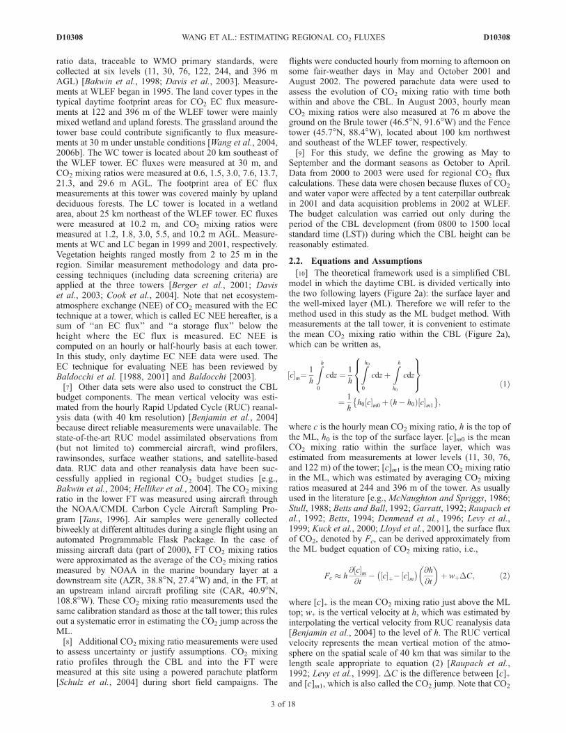
Figure 1. Location of the study site in northern Wisconsin, USA and land covers (represented bycolors) in the 60 � 60-km region centered on the WLEF tower. The three pluses represent the locations ofthe WC, LC, and WLEF towers. Land cover data source is WISCLAND [WiDNR, 1998].

D10308 WANG ET AL.: ESTIMATING REGIONAL CO2 FLUXES

2 of 18

D10308

ratio data, traceable to WMO primary standards, werecollected at six levels (11, 30, 76, 122, 244, and 396 mAGL) [Bakwin et al., 1998; Davis et al., 2003]. Measure-ments at WLEF began in 1995. The land cover types in thetypical daytime footprint areas for CO2 EC flux measure-ments at 122 and 396 m of the WLEF tower were mainlymixed wetland and upland forests. The grassland around thetower base could contribute significantly to flux measure-ments at 30 m under unstable conditions [Wang et al., 2004,2006b]. The WC tower is located about 20 km southeast ofthe WLEF tower. EC fluxes were measured at 30 m, andCO2 mixing ratios were measured at 0.6, 1.5, 3.0, 7.6, 13.7,21.3, and 29.6 m AGL. The footprint area of EC fluxmeasurements at this tower was covered mainly by uplanddeciduous forests. The LC tower is located in a wetlandarea, about 25 km northeast of the WLEF tower. EC fluxeswere measured at 10.2 m, and CO2 mixing ratios weremeasured at 1.2, 1.8, 3.0, 5.5, and 10.2 m AGL. Measure-ments at WC and LC began in 1999 and 2001, respectively.Vegetation heights ranged mostly from 2 to 25 m in theregion. Similar measurement methodology and data pro-cessing techniques (including data screening criteria) areapplied at the three towers [Berger et al., 2001; Daviset al., 2003; Cook et al., 2004]. Note that net ecosystem-atmosphere exchange (NEE) of CO2 measured with the ECtechnique at a tower, which is called EC NEE hereafter, is asum of ‘‘an EC flux’’ and ‘‘a storage flux’’ below theheight where the EC flux is measured. EC NEE iscomputed on an hourly or half-hourly basis at each tower.In this study, only daytime EC NEE data were used. TheEC technique for evaluating NEE has been reviewed byBaldocchi et al. [1988, 2001] and Baldocchi [2003].[7] Other data sets were also used to construct the CBL

budget components. The mean vertical velocity was esti-mated from the hourly Rapid Updated Cycle (RUC) reanal-ysis data (with 40 km resolution) [Benjamin et al., 2004]because direct reliable measurements were unavailable. Thestate-of-the-art RUC model assimilated observations from(but not limited to) commercial aircraft, wind profilers,rawinsondes, surface weather stations, and satellite-baseddata. RUC data and other reanalysis data have been suc-cessfully applied in regional CO2 budget studies [e.g.,Bakwin et al., 2004; Helliker et al., 2004]. The CO2 mixingratio in the lower FT was measured using aircraft throughthe NOAA/CMDL Carbon Cycle Aircraft Sampling Pro-gram [Tans, 1996]. Air samples were generally collectedbiweekly at different altitudes during a single flight using anautomated Programmable Flask Package. In the case ofmissing aircraft data (part of 2000), FT CO2 mixing ratioswere approximated as the average of the CO2 mixing ratiosmeasured by NOAA in the marine boundary layer at adownstream site (AZR, 38.8�N, 27.4�W) and, in the FT, atan upstream inland aircraft profiling site (CAR, 40.9�N,108.8�W). These CO2 mixing ratio measurements used thesame calibration standard as those at the tall tower; this rulesout a systematic error in estimating the CO2 jump across theML.[8] Additional CO2 mixing ratio measurements were used

to assess uncertainty or justify assumptions. CO2 mixingratio profiles through the CBL and into the FT weremeasured at this site using a powered parachute platform[Schulz et al., 2004] during short field campaigns. The

flights were conducted hourly from morning to afternoon onsome fair-weather days in May and October 2001 andAugust 2002. The powered parachute data were used toassess the evolution of CO2 mixing ratio with time bothwithin and above the CBL. In August 2003, hourly meanCO2 mixing ratios were also measured at 76 m above theground on the Brule tower (46.5�N, 91.6�W) and the Fencetower (45.7�N, 88.4�W), located about 100 km northwestand southeast of the WLEF tower, respectively.[9] For this study, we define the growing as May to

September and the dormant seasons as October to April.Data from 2000 to 2003 were used for regional CO2 fluxcalculations. These data were chosen because fluxes of CO2

and water vapor were affected by a tent caterpillar outbreakin 2001 and data acquisition problems in 2002 at WLEF.The budget calculation was carried out only during theperiod of the CBL development (from 0800 to 1500 localstandard time (LST)) during which the CBL height can bereasonably estimated.

2.2. Equations and Assumptions

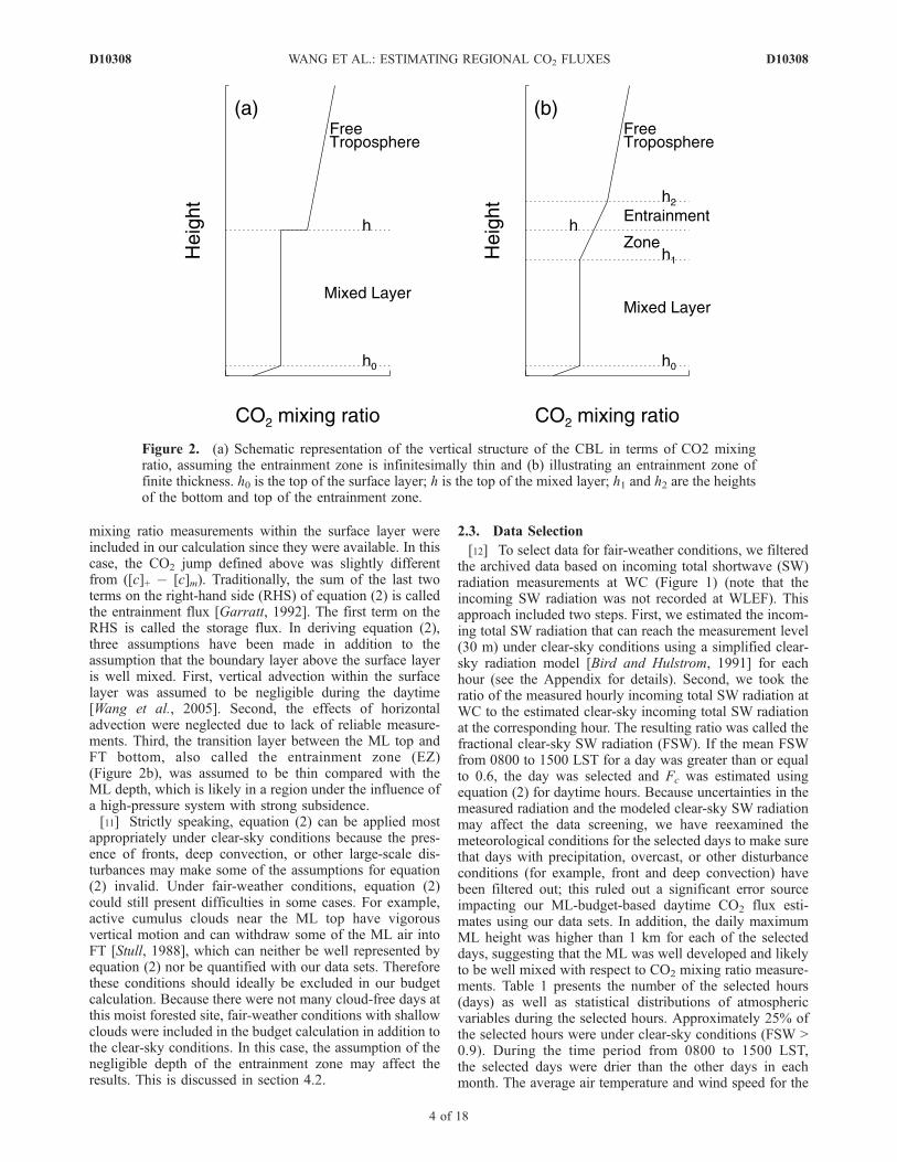
[10] The theoretical framework used is a simplified CBLmodel in which the daytime CBL is divided vertically intothe two following layers (Figure 2a): the surface layer andthe well-mixed layer (ML). Therefore we will refer to themethod used in this study as the ML budget method. Withmeasurements at the tall tower, it is convenient to estimatethe mean CO2 mixing ratio within the CBL (Figure 2a),which can be written as,

c½ �m¼1

h

Zh

0

cdz ¼ 1

h

Zh00

cdzþZh

h0

cdz

8><>:

9>=>;

¼ 1

hh0 c½ �m0 þ h� h0ð Þ c½ �m1

;

ð1Þ

where c is the hourly mean CO2 mixing ratio, h is the top ofthe ML, h0 is the top of the surface layer. [c]m0 is the meanCO2 mixing ratio within the surface layer, which wasestimated from measurements at lower levels (11, 30, 76,and 122 m) of the tower; [c]m1 is the mean CO2 mixing ratioin the ML, which was estimated by averaging CO2 mixingratios measured at 244 and 396 m of the tower. As usuallyused in the literature [e.g., McNaughton and Spriggs, 1986;Stull, 1988; Betts and Ball, 1992; Garratt, 1992; Raupach etal., 1992; Betts, 1994; Denmead et al., 1996; Levy et al.,1999; Kuck et al., 2000; Lloyd et al., 2001], the surface fluxof CO2, denoted by Fc, can be derived approximately fromthe ML budget equation of CO2 mixing ratio, i.e.,

Fc h@ c½ �m@t

� c½ �þ� c½ �m� � @h

@t

�þ wþDC; ð2Þ

where [c]+ is the mean CO2 mixing ratio just above the MLtop; w+ is the vertical velocity at h, which was estimated byinterpolating the vertical velocity from RUC reanalysis data[Benjamin et al., 2004] to the level of h. The RUC verticalvelocity represents the mean vertical motion of the atmo-sphere on the spatial scale of 40 km that was similar to thelength scale appropriate to equation (2) [Raupach et al.,1992; Levy et al., 1999]. DC is the difference between [c]+and [c]m1, which is also called the CO2 jump. Note that CO2


3 of 18

D10308

mixing ratio measurements within the surface layer wereincluded in our calculation since they were available. In thiscase, the CO2 jump defined above was slightly differentfrom ([c]+ � [c]m). Traditionally, the sum of the last twoterms on the right-hand side (RHS) of equation (2) is calledthe entrainment flux [Garratt, 1992]. The first term on theRHS is called the storage flux. In deriving equation (2),three assumptions have been made in addition to theassumption that the boundary layer above the surface layeris well mixed. First, vertical advection within the surfacelayer was assumed to be negligible during the daytime[Wang et al., 2005]. Second, the effects of horizontaladvection were neglected due to lack of reliable measure-ments. Third, the transition layer between the ML top andFT bottom, also called the entrainment zone (EZ)(Figure 2b), was assumed to be thin compared with theML depth, which is likely in a region under the influence ofa high-pressure system with strong subsidence.[11] Strictly speaking, equation (2) can be applied most

appropriately under clear-sky conditions because the pres-ence of fronts, deep convection, or other large-scale dis-turbances may make some of the assumptions for equation(2) invalid. Under fair-weather conditions, equation (2)could still present difficulties in some cases. For example,active cumulus clouds near the ML top have vigorousvertical motion and can withdraw some of the ML air intoFT [Stull, 1988], which can neither be well represented byequation (2) nor be quantified with our data sets. Thereforethese conditions should ideally be excluded in our budgetcalculation. Because there were not many cloud-free days atthis moist forested site, fair-weather conditions with shallowclouds were included in the budget calculation in addition tothe clear-sky conditions. In this case, the assumption of thenegligible depth of the entrainment zone may affect theresults. This is discussed in section 4.2.

2.3. Data Selection

[12] To select data for fair-weather conditions, we filteredthe archived data based on incoming total shortwave (SW)radiation measurements at WC (Figure 1) (note that theincoming SW radiation was not recorded at WLEF). Thisapproach included two steps. First, we estimated the incom-ing total SW radiation that can reach the measurement level(30 m) under clear-sky conditions using a simplified clear-sky radiation model [Bird and Hulstrom, 1991] for eachhour (see the Appendix for details). Second, we took theratio of the measured hourly incoming total SW radiation atWC to the estimated clear-sky incoming total SW radiationat the corresponding hour. The resulting ratio was called thefractional clear-sky SW radiation (FSW). If the mean FSWfrom 0800 to 1500 LST for a day was greater than or equalto 0.6, the day was selected and Fc was estimated usingequation (2) for daytime hours. Because uncertainties in themeasured radiation and the modeled clear-sky SW radiationmay affect the data screening, we have reexamined themeteorological conditions for the selected days to make surethat days with precipitation, overcast, or other disturbanceconditions (for example, front and deep convection) havebeen filtered out; this ruled out a significant error sourceimpacting our ML-budget-based daytime CO2 flux esti-mates using our data sets. In addition, the daily maximumML height was higher than 1 km for each of the selecteddays, suggesting that the ML was well developed and likelyto be well mixed with respect to CO2 mixing ratio measure-ments. Table 1 presents the number of the selected hours(days) as well as statistical distributions of atmosphericvariables during the selected hours. Approximately 25% ofthe selected hours were under clear-sky conditions (FSW >0.9). During the time period from 0800 to 1500 LST,the selected days were drier than the other days in eachmonth. The average air temperature and wind speed for the

Figure 2. (a) Schematic representation of the vertical structure of the CBL in terms of CO2 mixingratio, assuming the entrainment zone is infinitesimally thin and (b) illustrating an entrainment zone offinite thickness. h0 is the top of the surface layer; h is the top of the mixed layer; h1 and h2 are the heightsof the bottom and top of the entrainment zone.


4 of 18

D10308

selected hours were not significantly different from theirrespective monthly averages. For all the selected hours, themedian value of w+ estimated from the RUC reanalysisproduct was �0.008 ms�1 with the 25th and 75th percen-tiles being �0.02 and 0.003 ms�1, respectively (wherepositive value indicates upward motion). This suggests thatthe presence and growth of boundary layer clouds are limitedfor a majority of the selected hours. Note that the collectiveimpacts of possible large-scale subsidence, cloud dynamics,local circulations, and other processes on the atmosphericvertical motion have been taken into account in the use of theRUC model [Benjamin et al., 2004].

2.4. Estimating the ML Height, h

[13] Two methods were combined to estimate h becauseof the lack of routine direct measurements. Observationalstudies have suggested that the growing ML top and thelifting condensation level (LCL) may be coupled and growtogether under fair-weather conditions as small cumulusbegin to form over moist terrain like our forested site [e.g.,Stull, 1988; Betts, 1994; Parasnis and Morwal, 1994]. As aresult, the LCL of the ML air could be a good approxima-tion for the ML height, particularly over moist areas [Betts,1994, 2000; Betts et al., 2004]. This approximation, how-ever, may not be always true. For example, when the ML airis dry, the LCL can be very high and the ML top may not beable to reach the LCL because the ML growth is limited byother factors such as surface heating and entrainment. In thiscase, the ML height cannot be approximated to be the LCLheight and needs to be estimated with other methods. Thereare many theoretical or empirical models for estimating h inthe literature [e.g., Tennekes, 1973; Stull, 1988; Garratt,1992; Batchvarona and Gryning, 1994]. In this study, weadopted an empirical model derived from radar measure-ments at this study site [Yi et al., 2001]. The ML height wasfirst estimated from this model and then adjusted to the LCLheight if the LCL was less than the first estimate. See theAppendix for the empirical formulas for the ML [Yi et al.,2001] and LCL [Betts, 2000] heights. Figure 3 shows themonthly diurnally averaged ML heights for the selecteddays in our budget calculation. In general, the ML heightwas lowest in August when the ML air was most moist. The

Figure 3. Estimated monthly diurnally averaged MLheights for the selected days. There are insufficient data pointsto calculate diurnally averaged ML heights for December,January, and February.T

able

1.DistributionofAtm

ospheric

VariablesfortheSelectedHoursa

Month

Hours

(Days)

FSW

PAR(mmolm

�2s�

1)

w(cm/s)

AirTem

perature

(�C)

WindSpeed(m

/s)

RelativeHumidity(%

)

Median(Q

1,Q3)

March

andNovem

ber

98(12)

0.85(0.69,0.93)

925(583,1189)

�0.32(�

1.08,0.42)

�4.8

(�10,4.9)�3.4

(�11,1.70)b

4.2

(2.6,4.9)3.7

(2.7,5.0)b

57(45,81)81(63,94)b

April

112(13)

0.84(0.69,0.92)

1400(1039,1620)

�1.06(�

1.90,0.02)

3.9

(1.9,12.2)5.0

(0.2,11.2)b

4.0

(2.5,5.3)3.8

(2.7,5.2)b

37(26,50)56(34,87)b

May

229(26)

0.86(0.74,0.94)

1564(1281,1784)

0.08(�

1.73,1.55)

16.3

(13.7,19.5)14.3

(10.4,17.9)b

3.9

(3.2,4.9)3.7

(2.7,4.9)b

43(34,58)56(39,81)b

June

202(23)

0.86(0.68,0.94)

1524(1246,1725)

�0.70(�

1.82,0.25)

18.4

(15.5,20.8)17.0

(13.2,20.4)b

3.2

(2.5,4.0)3.0

(2.2,4.0)b

57(43,71)75(52,94)b

July

214(28)

0.81(0.65,0.92)

1478(1214,1771)

�0.65(�

1.90,0.74)

22.8

(19.2,24.6)20.7

(17.4,23.6)b

3.2

(2.2,4.4)3.1

(2.2,4.1)b

63(53,75)73(58,88)b

August

242(30)

0.86(0.77,0.93)

1460(1160,1630)

�0.97(�

1.89,0.05)

22.1

(19.1,24.0)20.7

(17.6,23.4)b

2.9

(2.1,4.0)2.9

(2.1,3.8)b

66(55,83)74(60,91)b

September

210(26)

0.86(0.71,0.93)

1152(830,1428)

�0.91(�

2.07,�0.04)

14.8

(11.1,21.0)15.6

(10.1,20.2)b

3.1

(2.3,4.3)3.6

(2.6,4.7)b

60(47,73)69(53,92)b

October

111(15)

0.80(0.69,0.91)

926(713,1148)

�1.21(�

2.09,�0.21)

10.5

(5.10,19.3)9.0

(3.90,14.9)b

4.3

(3.1,5.2)3.7

(2.6,4.6)b

62(52,73)72(53,94)b

aEachdistributionisrepresentedbythe25th

(Q1),50th

(median),and75th

(Q3)percentilesoftheatmosphericvariable.Medianvalues

arebold.FSW

=fractionalclear-skyshortwaveradiationreaching30m

ofthe

WCtower.PARisphotosynthetically

activeradiation.wisthemeanverticalvelocity

inunitsofcentimetersper

second.Airtemperature,windspeed,andrelativehumidityweremeasuredat30m

oftheWLEFtower.

bThesecondmedian(Q

1,Q3)in

each

cellshowsstatisticaldistributionofthevariable

duringalldaytimeofthecorrespondingmonth

(incomparisonwiththat

duringtheselected

hours).Noprecipitationwas

recorded

fortheselected

hours.


5 of 18

D10308

ML height was highest in April and May. More discussionsabout the ML in the region can be found in the work of Yiet al. [2001]. The ML top usually reached the LCL height inthe afternoon. The LCL height was used to approximate theML height for 89% of the selected hours in the moist monthof August, suggesting that the influence of small cumulusnear the ML top on our budget calculation [equation (2)]might be significant. In contrast, the LCL height was usedfor only 34% of the selected hours in the dry winter month.

2.5. Estimating CO2 Jump

[14] In the literature, [c]+ is usually approximated to bethe baseline or FT mixing ratio [Raupach et al., 1992;Denmead et al., 1996] or the mixing ratio measured atoceanic sites [Levy et al., 1999] when direct measurementsare unavailable. Such approximations, however, can resultin significant errors when an air mass has passed over thecontinent for a long time [Levy et al., 1999]. As a result, it isinappropriate to use those approximations at our continentalsite as shown in Figure 4 and indicated from earlier studies[Helliker et al., 2004; Yi et al., 2004].[15] To a first-order approximation, we proposed a method

to estimate [c]+ via a combination of CO2 mixing ratiomeasurements at the tall tower and aircraft profile measure-ments in the lower part of the FT.When theML top was lowerthan 396 m, measurements at WLEF can be used as anestimate of [c]+. When the ML top was higher than 396 m,[c]+ was estimated with the following equation,

@ c½ �þ@t

@C

@z

�þ

@h

@t� wþ

�; ð3Þ

which follows a derivation by Tennekes [1973]. We haveused the following common assumptions. First, horizontaladvection above the ML was negligible compared withvertical advection. Second, the time rate of change in CO2

mixing ratio above the ML was small compared with thatwithin the ML, which can be justified by the observedevolution of CO2 mixing ratio profiles within and above theML under fair-weather conditions (powered parachuteobservations in Figure 4 for example). (@C/@z)+ is thevertical gradient of CO2 mixing ratio just above the ML;this vertical gradient can be nearly invariant with height in alimited layer above the ML to a certain height in the lowerFT.[16] The measured CO2 mixing ratio profiles above the

ML showed that the CO2 mixing ratio generally decreasedwith height above the ML in the dormant season due to thenet release of CO2 by ecosystems, while increasing withheight in the growing season due to the net uptake of CO2

on the surface. The lines in Figure 4 show examples of CO2

mixing ratio profiles above the ML in spring, summer, andautumn. The tropospheric profiles may not be well mixedbecause the exchange of CO2 between the atmosphericboundary layer and lower FT by turbulent transport is notas efficient as mixing within the ML. Sometimes the CO2mixing ratio above the ML can be observed to be nearlyinvariant with height during or shortly after synoptic dis-turbances such as fronts and deep convections due to large-scale mixing [Hurwitz et al., 2004].[17] To examine if the CO2 mixing ratio can be approx-

imated to vary linearly with height above the ML, we fittedthe CO2 mixing ratio as a linear function of height above theML to 3500 m for each of the available vertical profiles ofCO2 mixing ratio from the powered parachute flights underfair-weather conditions. The coefficients of the determina-tion (r2) were calculated to assess how well the linearfunction can explain the variation of CO2 mixing ratio withheight above the ML. We divided the powered parachuteprofiles into two categories. In the first category, the CO2

mixing ratio can be approximated to be invariant withheight compared to the CO2 jump across the ML top whenthe magnitude of the variation of CO2 mixing ratio withheight (i.e., the magnitude of the slope in the linearequation) was smaller than 0.2 ppm/1 km. In this case,the variation in CO2 mixing ratio with height above the MLto 3500 m was difficult to measure accurately due to thelimited precision (about 0.5 ppm) of the instruments.Twenty-one out of the total 54 observed profiles fell intothis category. The rest (33) of the profiles fell into thesecond category where the CO2 mixing ratio changedsignificantly with height above the ML, that is, the magni-tude of slope was greater than 0.2 ppm/1 km. In this case,the linear function can explain more than 80% (r2 > 0.8) ofthe variation in CO2 mixing ratio with height for 29 of the33 cases.[18] On the basis of this analysis, we approximated the

CO2 mixing ratio gradient to a first order as,

@C

@z

�þ

c½ �þ�CH

h� H; ð4Þ

where H was taken as 3500 m from the data analyses in thisregion; CH is the CO2 mixing ratio at H for a given time,which was estimated by fitting the averaged NOAA/CMDL

Figure 4. Examples of vertical profiles of CO2 mixingratio from near the surface through the lower FT measuredat the WLEF site. Symbols indicate measurements from thepowered parachute campaign [Schulz et al., 2004], showingevolution of the profile with time for a day in summer. Linesare based on NOAA/CMDL aircraft measurements, show-ing typical vertical profiles of CO2 mixing ratio in spring(solid line), summer (dashed line), and autumn (dot-dashedline). LST stands for local standard time. CO2 mixing ratioat 3.5 to 4 km can be approximated as the baseline mixingratio, which can be significantly different from the mixingratio just above the ML (ML heights are about 1–1.2 km forthe days shown).


6 of 18

D10308

aircraft measurements between 3 and 4 km as a function oftime. The value of [c]+ estimated from tall tower measure-ments provided the initial condition for equation (3) as theML was developing and close to the top level of the talltower in the morning of a given day. By solving equation (3),the CO2 jump was estimated during the developing period ofthe fair-weather ML (from 0800 to 1500 LST) (Figure 5).The CO2 jump was negative during the dormant season,implying that the CO2 mixing ratio was smaller above thanwithin the ML. In contrast, the jump was positive during thegrowing season (solid lines in Figure 5). During the dormantseason, the jump did not vary significantly with month andwith time of day. During the growing season, the jumpvaried significantly both with month (mostly due to changesin phenology) and with time of day (in response to diurnalchanges in photosynthetically active radiation (PAR)). Ingeneral, the magnitude of the CO2 jump was larger in thesummer months than in the months of late spring and earlyautumn. The variation in the jump from morning tomidafternoon was the largest in summer. CO2 mixing ratiocan be tens of parts per million larger below than above theML in the early morning [Yi et al., 2004] (not shown here) asa result of the very high concentration of respired CO2

accumulated near the surface in summer. With PARincreasing from morning to middle afternoon, CO2 withinthe ML was rapidly assimilated by photosynthetic uptake,leading to a large positive jump in the middle afternoon. Inother months during the growing season, the variation in thejump from morning to afternoon was smaller mainly due toweaker assimilation and respiration rates. It should be kept inmind that likely impacts of the residual boundary layer andclouds above the ML top have not been considered in thisfirst-order estimate. More studies are needed in the future toimprove the estimates of [c]+. Nevertheless, our estimates for[c]+ were an improvement on those approximated as FTvalues in earlier studies.

2.6. Estimating Terms in Equation (2)

2.6.1. Entrainment Flux Term[19] The entrainment flux, characterizing the net exchange

of CO2 across the ML top, can be estimated as,

Fe ¼ � c½ �þ� c½ �m� � @h

@tþ wþDC; ð5Þ

where the first term on the RHS represents the exchanges ofCO2 due to the varying ML top, and the second termrepresents changes due to vertical advection. Both termswere of the same order of magnitude (Figure 5). Diurnalchanges in the first term are determined by the variationsboth in the CO2 jump and in h with time. Diurnal changes inthe second term are correlated mainly with those in the CO2

jump because the vertical velocity did not significantly varydiurnally compared to the CO2 jump. In addition, thediurnal patterns of changes in the ML height and the verticalvelocity (Table 1) did not vary significantly with seasoncompared with that in the CO2 jump. As a result, theseasonal change in the diurnal cycle of each of the twoterms in equation (5) was determined primarily by that ofthe CO2 jump.[20] The monthly diurnally averaged entrainment flux

(Fe) is presented in Figure 6. The magnitude of the

entrainment flux from 1000 to 1500 LST during the growingseason was about 50% of the surface flux in May andSeptember and increased to 80% in summer months. In theearly morning, the entrainment flux value can have anopposite sign to the surface flux due to the negative CO2

jump (Figures 5 and 6c, 6f, and 6g). During the dormantseason, the magnitude of the entrainment flux term waslarger than that of the surface flux. This large percentage ofthe entrainment flux relative to the surface flux suggests thataccurately quantifying the entrainment flux at the ML top isimportant in improving regional CO2 flux estimates.2.6.2. Storage Flux Term[21] In general, the mean mixing ratio of CO2 in the CBL

decreased with time as the CBL grew from morning to earlyafternoon at this site for all months, resulting in the storageflux term being negative. We noticed that this term was onlyslightly more negative in the growing season, despite muchstronger CO2 uptake at the surface, than in the dormantseason (Figure 6). This was because the influence of surfaceCO2 fluxes on the atmospheric CO2 mixing ratio within theCBL was modulated significantly by the dynamics of thedaytime CBL [Denning et al., 1999; Gurney et al., 2002].The storage flux (in the midday) was about 20% of thesurface flux in June, July, and August and 50% in May andSeptember. Overall, the storage flux term had the same signas Fc during the growing season, but had the opposite signand larger magnitude during the dormant season. Morenotably, the storage flux term had similar magnitude butan opposite sign to the entrainment flux term during thedormant season unlike during the growing season, suggest-ing that the estimated regional daytime CO2 flux (whichwas the sum of the two terms) was subject to moresignificant errors.

3. Results and Discussion

3.1. Diurnal Average of Daytime Regional CO2 Fluxand Comparisons With EC Measurements at ThreeLevels of the WLEF Tower

[22] During the dormant season (Figures 6a, 6b, and 6h),the estimated daytime regional CO2 flux was generallypositive from 0800 to 1500 LST and smaller from latemorning to early afternoon than other periods of time in theday due to photosynthetic activity of coniferous forests inthe region. Compared with the dormant season, the estimateddaytime CO2 flux was significantly negative during thegrowing season with the largest net uptake of CO2 beingfound in June and July. The magnitude of the estimateddaytime regional CO2 flux was generally larger in themidday hours than in the early morning (for example,0800 LST) and midafternoon (for example, 1500 LST).[23] The estimated daytime regional CO2 flux was com-

parable to daytime EC NEE measured at 396 m of theWLEF tower (open circles in Figure 6). In Figure 6 as wellas in Figure 7, EC NEE had been chosen for the same hoursas the ML-budget-derived daytime regional CO2 flux couldbe calculated. Daytime EC NEE values measured at higherlevels of the tall tower were generally closer to the budget-derived daytime regional CO2 fluxes (Figure 7). This can beexplained in part from the footprint perspective. Footprintmodeling suggests the fractional weights (or contributions)from the ecosystem types in the source areas for higher-


7 of 18

D10308

level EC measurements were closer to the fractional areas ofthe respective ecosystem types in the larger 40 � 40 km2

region [Wang et al., 2004; Wang et al., 2006a]. As a result,daytime EC NEE values measured at the two higher levelsmay approximate daytime regional CO2 flux better thanthose at the lowest level, assuming that all ecosystem typesin the footprint areas are representative of the entire region.

3.2. Responses of Daytime Regional CO2 Flux to PARand Temperature and Comparisons With ECMeasurements at Three Towers

[24] We examined the responses of the estimated daytimeregional CO2 flux to PAR and to air temperature, respec-tively. To reduce random errors, daytime regional CO2 flux

Figure 5. Diurnal average CO2 jump (DC=[c]+�[c]m), vertical advection term (w+DC), andentrainment flux component due to changes in ML top (�DC@h/@t) from 0800 to 1500 LST for eachmonth. There are insufficient data for analyses in December, January, and February. The CO2 jump (solidline) is scaled by the left axis, while other variables are scaled by the right axis. The error bars are thestandard deviations of the means.


8 of 18

D10308

values were binned by PAR in increments of 200 mmolquanta m�2 s�1 starting from zero. The mean flux and itsstandard deviation were calculated for each bin. Figure 8presents the bin-averaged ML-budget-derived daytimeregional CO2 flux, along with those daytime EC NEEmeasurements at WC, LC, and WLEF, as a function of

PAR in each month. Note that all available daytime ECNEE measurements were used in the calculation. Theanalysis in section 4.4 suggests that differences in CO2 fluxunder the selected weather conditions and under all weatherconditions could be negligible for a given PAR bin duringthe growing season. The magnitude of daytime EC NEE

Figure 6. Diurnal averages of the calculated daytime regional flux, entrainment flux, and storage fluxfrom 0800 to 1500 LST for each month. The diurnal average EC NEE measured at 396 m of the WLEFtower for the same hours is shown as circles for comparison. The 396-m daytime EC NEE was notavailable in March, April, and November when the ML-budget-derived flux was available. There are notsufficient data for analyses in December, January, and February. The error bars show the standarddeviations of the means.


9 of 18

D10308

measured at WC was the largest for a given PAR valueamong all estimates during the growing season with excep-tion of the month of May (when leaves were just starting togrow), while the magnitude of daytime EC NEE measured atLC was the smallest. Daytime regional CO2 flux estimateswere intermediate and, overall, the closest to daytime ECNEE measured at 396 m of the WLEF tower.[25] In addition, daytime EC NEE measurements at indi-

vidual stand towers showed that the ecosystem CO2 fluxesfor individual stand types tended to saturate in June, July, andAugust when PAR exceeded 1000 mmol quanta m�2 s�1

(Figure 8). In contrast, such saturation did not appear in thedaytime regional CO2 flux as shown in Figure 8. This wasconsistent with earlier findings that scaling up in time orspace might ‘‘linearize’’ the light response curve anddecrease the apparent quantum yield [Ruimy et al., 1995].[26] To estimate and integrate daytime regional CO2 flux

over long periods of time such as months, we tried fittingthe estimated regional flux to ecosystem models that for-mulate CO2 fluxes as a function of PAR or air temperature.Because the ML budget method was applied only from0800 to 1500 LST under fair-weather conditions, theresulting flux estimates were associated with a range oflarge PAR values. When the ML-budget-based daytime CO2

flux estimates were unavailable for the given PAR values,daytime EC NEE measured at 396 m of the WLEF towerwas used to approximate the regional flux. This was

because the 396-m daytime EC NEE was likely the closestto the regional flux among the flux tower measurementsbased on comparisons in previous sections. As a result, theresponse of the estimated daytime regional CO2 flux to PARcan be modeled with a rectangular hyperbolic relationship[Ruimy et al., 1995],

Fc ¼aIPm

aI þ Pm

þ R ð6Þ

where I is PAR (mmol quanta m�2 s�1); Pm (mmolC m�2 s�1)is the saturated assimilation rate; a is the apparent quantumyield (mmolC/mmol quanta), and R is the intercept that can beinterpreted as the daytime respiration rate (mmolC m�2 s�1).During the growing season, variations in the estimateddaytime regional CO2 flux with PAR can be describedreasonably by the light response curve. Overall, the mag-nitude of the apparent quantum yield for the regional flux wassmaller than when fitted frommeasurements at individual ECtowers; this is consistent with the implication of the study byRuimy et al. [1995]. The magnitude of the saturatedassimilation rate (Pm) for the regional flux was intermediateamong those fitted from measurements at individual ECtowers, with WC having the largest value. The regional fluxrespiration rate (R) is also intermediate in value, with WLEFhaving the largest value and LC having the smallest.[27] The response of daytime regional CO2 flux to PAR,

however, cannot be well described by the light responsemodel (Figures 8a, 8b, and 8h) during the dormant season asa result of significantly reduced photosynthetic activities.Therefore we also examined the relationship between eco-system CO2 flux and air temperature. The estimated day-time CO2 flux values were binned by the air temperaturemeasured at 30 m of WLEF in increments of 4�C. Figure 9shows the bin-averaged daytime regional CO2 flux as afunction of the air temperature, suggesting that daytimeregional CO2 flux estimates were generally intermediateamong the daytime EC NEE values for a given air temper-ature during the dormant season. The response of daytimeregional CO2 flux to air temperature was modeled with anexponential equation, i.e.,

Fc ¼ aebT ; ð7Þ

where T is the air temperature at 30 m in degrees Celsiusabove the ground, a is SF at T = 0�C, and b is the coefficientdescribing the sensitivity of the flux to the change intemperature. The equation is identical mathematically to thewidely used Q-10 model [Lloyd and Taylor, 1994]. Onlyabout 30% (r2) of the variation of the estimated daytimeregional CO2 flux with air temperature can be explained bythe exponential model. Two reasons may account in part forsuch a low value of r2. First, relative errors in regional fluxestimates were generally larger during the dormant seasonthan during the growing season due to the smallermagnitude of the flux as discussed in section 2.6. Second,the ML budget method aggregated the fluxes for all standtypes including deciduous and coniferous forests in theregion and, hence, neither the respiratory process nor theassimilation process overwhelmingly dominated in the day

Figure 7. Comparison of the monthly diurnally averageddaytime regional flux inferred from the ML budget method(x axis) and daytime EC NEE measured at the three levels ofthe WLEF tower (y axis). The variables y30, y122, and y396 inthe linear equations represent daytime EC NEE measured at30, 122, and 396 m of the WLEF tower, respectively, whilex represents daytime regional CO2 flux derived from theML budget method. Note that EC NEE values wereaveraged over the same hours as the ML budget calculationsand EC NEE is a sum of EC flux at a height and storage fluxbelow the height.


10 of 18

D10308

Figure 8. (a) Bin-averaged daytime CO2 flux values inferred from the ML budget method and directlymeasured with the EC technique at WC, LC, and WLEF as a function of PAR in November and March,(b) April, (c)May, (d) June, (e) July, (f) August, (g) September, (h) October. There are insufficient data to showfor December, January, and February. Data are binned by PAR in increments of 200 mmol quanta m�2 s�1.The standard deviation is for the mean flux in each bin. r2 is the coefficient of determination, indicating thedegree to which the change in bin-averaged flux with PAR can be explained by the fitted curve (thick greylines).


11 of 18

D10308

on the regional scale during the dormant season. This likelyled to the difficulty in describing daytime regional CO2 fluxonly with either the light response model or the exponentialmodel. In other words, both temperature and PAR may beamong the important factors controlling the daytimeecosystem CO2 flux in the region. In contrast, for individualstands, temperature or PAR can be the dominant factorcontrolling ecosystem CO2 flux, and therefore, changes inthe flux with environmental conditions can be explainedreasonably by one of the ecosystem models (equations 6and 7).

3.3. Monthly Averaged Daytime-Integrated RegionalCO2 Flux and Comparisons With EC Measurements

[28] We hypothesized that the ecosystem models fitted tothe ML-budget-derived daytime regional CO2 flux underthe selected weather conditions can represent those underall weather conditions. The possible bias is discussed insection 4.4. With this hypothesis, daytime regional CO2 fluxof each hour was calculated using equations (6) and (7) withmeasured PAR and air temperature at WLEF, then integratedover the daytime hours for each day. Missing hourly PARand temperature data were approximated as their respectivemonthly diurnally averaged values. For comparison, thehourly EC NEE at each flux tower was also integrated overthe daytime hours, where the monthly diurnally averagedEC NEE values were used for filling the missing measure-ments. The daytime-integrated regional CO2 flux (DIRF)derived from the budget method was intermediate amongthose estimated from EC NEE measurements (Figure 10).The error bounds in the figure are the standard deviationsof the mean DIRFs plus the average errors (due to modeluncertainty), where we have assumed DIRFs and theirerrors are independent for different days, respectively. Notethat possible systematic errors are not included in the error

bounds. The average DIRF was estimated to be about 0.35 ±0.18 gC m�2 during the dormant season, suggesting that theregion was likely a small net source of CO2 in the daytime.In the dormant season, significant differences between theDISF values and daytime EC NEE measurements were notfound due to large uncertainties relative to flux magnitudes.The region was a significant net sink in the daytime duringthe growing season with the maximum net uptake (�4.51 ±0.32 gC m�2) occurring in June (Figure 10). ML-budget-derived daytime regional flux values are in between thosederived from EC measurements at different towers or levels.DIRF values were closest to those from EC measurements at396 m of WLEF in June, July, and August. This may not betrue for other months. These comparisons and the largevariability in DIRF values and EC measurements suggestthat the responses of stands to similar environmental con-ditions over the region are significantly different, andtherefore, it is not appropriate to use EC NEE measurementsat any single stand tower to describe the region. Next, wewill further compare ML-budget-derived DIRF to thoseestimated from independent methods.

3.4. Comparisons With Other Regional CO2 FluxEstimates

[29] Regional fluxes can be estimated using differentmethods. Although each method may have limitations (thatmight result in systematic errors), it is instructive to con-struct a variety of regional CO2 flux estimates. Table 2compares the daytime regional CO2 flux estimated from theML budget method with those from three aggregationexperiments for this region reported in the literature. Ineach of the aggregation experiments, the ecosystem wasclassified based on land cover types derived from the

Figure 9. Bin-averaged daytime CO2 fluxes derived fromthe ML budget method and directly measured with the ECtechnique at the three towers as a function of air temperatureat 30 m (except for the LC tower where air temperature wasmeasured at 10 m) during the dormant season from Octoberto April. Data are binned by air temperature in increments of4�C. Note that EC NEE data were not available in Januaryand February and the budget-derived flux was unavailablefrom December through February. The error bars are thestandard deviations of the means.

Figure 10. Comparison of monthly averaged daytime-integrated CO2 flux derived from the ecosystem modelsfitted to the ML-budget-derived flux and measured with theEC technique at WC, LC, and three levels of the WLEFtower in 2000 and 2003. Data are available only in 2003 atthe LC tower. ‘Dormant,’ data points are averaged resultsfor months from October to April (i.e., dormant season).The error bars are the standard deviations of the means(of daytime-integrated fluxes).


12 of 18

D10308

WISCLAND database [WiDNR, 1998]. Regional CO2 fluxwas then estimated as the area-weighted average of the CO2

flux values for the respective ecosystem types over a 40 �40 km2 region centered at WLEF. The three aggregationexperiments are briefly described and discussed as follows.[30] In the first experiment, the entire ecosystem was

classified into wetland and upland on the basis of watershedfunctions [Wang et al., 2006a]. Wetland and upland eco-system CO2 fluxes were assumed to be represented by themeasurements at LC and at WC, respectively. Measure-ments in 2000 and 2003 were used. Note that measurementsat LC in 2000 were unavailable and were approximated asthose in 2003 in the aggregation calculation. This aggrega-tion might overestimate the net uptake of CO2 in summersince daytime CO2 fluxes measured at both sites could besignificantly higher in magnitude than those estimated ormeasured for other upland forest and wetland sites [Wanget al., 2006a; Desai et al., 2007]. In other words, measure-ments at WC and LC cannot represent all upland forests andwetlands in the region.[31] In the second experiment, the entire ecosystem was

classified into six stand types and CO2 flux for each typewas inferred by decomposing EC fluxes measured at WLEFinto stand-type contribution using footprint models [Wanget al., 2006a]. The inferred CO2 flux values for the sixecosystem types were assumed to represent the entireregion. Measurements in 2000 and 2003 were used. Forsimilar land cover types, respiration rates were likely higherin the source area of flux measurements at WLEF than otherareas in the region according to analyses by Desai et al.[2007] and Wang et al. [2006a]. As a result, aggregationresults from this experiment might underestimate the day-time net CO2 flux in the region.[32] In the third experiment, the entire ecosystem was

classified into 14 stand types in a similar effort to estimateregional NEE in the same region [Desai et al., 2007].Regional CO2 flux values for each of the ecosystem typeswere assumed to be represented by measurements at an ECflux tower of the corresponding stand type located in anextended region across the upper midwest of USA. Mea-surements from June to August 2003 were used. Whethermeasurements at stand-level towers outside the region canrepresent the studied region or not was a major source ofuncertainty in this experiment.

[33] In general, daytime regional CO2 fluxes derived fromthe budget method were reasonably comparable to thosefrom the aggregation experiments. A number of reasonsmay account for differences in the regional flux estimates.Three of them are discussed here.[34] First, the budget-based method suffers from nonuni-

form time-varying source areas and land cover percentagesover the areas within a heterogeneous ecosystem. Althoughthe size of the source area is of the same order as that of theregion over which the aggregation experiments were made,it is hard to accurately quantify the land cover percentages(over the source area) that may change with meteorologicalconditions.[35] Second, how well the EC NEE measurements for

individual ecosystem types (based on a given classificationscheme) on local scales are representative of the studiedregion is uncertain and challenging to verify. This issuearises not only because of flux measurement errors them-selves, but also because of the selection of classificationschemes [Wang et al., 2006a]. A widely used ecosystemscheme is based on land cover types. Ecosystem CO2

fluxes, however, are also dependent on other ecosystemfeatures such as soil types, stand ages, forest management,and canopy density [Wirth et al., 2002; Euskirchen et al.,2003; Litvak et al., 2003; Litton et al., 2004; Wang et al.,2006a; Desai et al., 2007]. More detailed classificationschemes, which are not limited to land cover types, maybe needed to more accurately estimate regional fluxes withaggregation methods.[36] Finally, surface fluxes derived from the one-

dimensional tower-based EC system and from theML budgetmethod are subject to systematic errors associated withassumptions used, which may lead to biased estimates.Uncertainties in EC NEEmeasurements have been discussedextensively in the literature [e.g., Goulden et al., 1996;Moncrieff et al., 1996; Mahrt, 1998]. Next, we discussuncertainties in the ML budget calculation.

4. Uncertainties

4.1. Uncertainties due to use of Measurements at theSingle Location

[37] The vertical profiles of CO2 mixing ratio measured ata single location, which were assumed implicitly to berepresentative of the region, were used to calculate thestorage flux term and the entrainment flux term. We

Table 2. Comparison of Daytime-Integrated Regional CO2 Flux Estimates (gCm�2) From Different Methods

Methods Month

Aggregation Experiments

ML-Budget MethodLC and WC Aggregation Decomposition and Aggregationa Multitower Aggregationb

May �0.88 ± 0.22 �2.09 ± 0.42 N/A �1.58 ± 0.19June �5.44 ± 0.26 �3.90 ± 0.70 �4.17 ± 1.0 �4.51 ± 0.32July �6.66 ± 0.24 �4.04 ± 0.76 �5.29 ± 1.2 �4.35 ± 0.29August �5.71 ± 0.21 �2.91 ± 0.76 �4.42 ± 1.2 �3.47 ± 0.24September �2.76 ± 0.25 �1.43 ± 0.47 N/A �2.25 ± 0.24Dormant Season 0.37 ± 0.19 N/A N/A 0.35 ± 0.18

aAggregation experiments were conducted only during the growing season [Wang et al., 2006a].bMultitower aggregated scaling experiment was made using data during summer in 2003 [Desai et al., 2007]. The estimated errors do not include the

uncertainties due to the assumptions or simplifications used in the respective methods as well as land cover distribution errors (which might lead tosystematic errors in estimated regional flux). N/A indicates that results are not available.


13 of 18

D10308

compared the time rate of change of CO2 mixing ratiomeasured at 76 m of the WLEF tower, Brule tower, andFence tower in the daytime under fair-weather conditions inAugust 2003. The time derivative at the WLEF site deviatedfrom the average of those at the three towers, on average, by0.0012 ± 0.0007 mmol m�3 s�1, where the error bound is thestandard deviation of the mean. With a typical ML height of1000 m, the monthly average error in the storage flux due tosampling at a single location was about 1.2 mmol m�2 s�1,assuming that the time derivative of the mean CO2 mixingratio in the whole CBL can be approximated by the 76-mmeasurement [Yi et al., 2001]; this error was about 10% ofthe daytime CO2 flux in magnitude.[38] For the entrainment flux term, we can only make a

crude evaluation because observational data of the horizon-tal gradients of CO2 mixing ratio are unavailable. Providedthat the difference of CO2 mixing ratio was about 1 to2 mmol mol�1 over a horizontal distance of 40 km in the dayunder fair-weather conditions during the growing seasonand that the horizontal gradient of CO2 mixing ratio abovethe ML top was negligible compared with that within theCBL, the resulting error in the entrainment flux term wouldbe 0.4 to 0.7 mmolC m�2 s�1 in the afternoon given that thegrowth rate of the ML depth was negligible and the meanvertical velocity was �0.01 ms�1. This error was negligiblecompared to the typical daytime CO2 flux magnitude of15 mmol m�2 s�1 in the growing season. During the devel-oping period of the ML, the error, however, would be largerdue to the large entrainment velocity. For instance, with anincrease of 200 m in the ML depth per hour occurring in themorning, the error would be about 2 to 4 mmol m�2 s�1,which was about 10 to 20% of the daytime regional CO2 fluxestimate.

4.2. Effects of the Entrainment Zone at the top of ML

[39] The depth of the entrainment zone (EZ) at the top ofML was neglected in estimating the surface flux. Typically,the fair-weather EZ is about 20% of the mean depth of theML as indicated by observations [e.g., Davis et al., 1997].We evaluated the changes of the storage flux and entrain-ment flux terms in equation (2) when a finite EZ depth wastaken into account. We assumed that the EZ depth was aconstant fraction (20%) of the ML depth. To facilitatecalculation, the CO2 mixing ratio was assumed to varylinearly with height within the EZ and the mean height ofthe ML top was in the middle of the EZ (Figure 2b). Withthe finite EZ, the monthly average of the storage flux termincreased by approximately 10% of the magnitude of thesurface flux compared with that with no EZ during thegrowing season. This was offset by a decrease of similarmagnitude in the monthly average of the entrainment fluxterm. In the dormant season, there was a similar balance inthe decrease of the storage flux and increase of the entrain-ment flux as a percentage of the magnitude of the surfaceflux. Even if the EZ depth was doubled, the relative changein daytime regional CO2 flux estimates was still smalldespite the resulting change of each term increasing by afactor of about 1.5 to 2.[40] For an extreme case where the bottom of EZ was

located at the ML top (i.e., h1 = h in Figure 2b), a differencein daytime regional CO2 flux with and without the EZ beingconsidered would be about 10% if the EZ depth was

assumed to be 20% of the ML depth. In other words, CO2

uptake and release may be underestimated by 10% duringboth growing and dormant seasons under this extremecondition. Note that the effects of the EZ on the CO2 jump(the difference in CO2 mixing ratio at h1 and h2 in this case)had been considered in this evaluation.

4.3. Effects of Horizontal Advection

[41] Direct evaluation of the horizontal advection term inthe budget equation requires high-precision measurementsof horizontal distribution of CO2 mixing ratio, which is notavailable without an array of instruments. Attempts havebeen made to estimate the effects of the horizontal advectionusing the spatial distribution of water vapor mixing ratio[Wang, 2005]. A brief summary is given here.[42] The effects of horizontal advection on daytime

regional CO2 flux estimates due to the heterogeneousdistribution of the surface vegetation at this site werepreliminarily assessed on a 40-km scale in eight winddirection sectors. The overall magnitude of the effects wasless than 15–20% of the flux in each wind direction inthe early afternoon (from noon to 1500 LST) during thegrowing season. When the winds were from the northeast,east, and southeast directions, the horizontal advective

fluxes (Rh0

U(@c/@x)dz, where U is the horizontal wind speed;

x is the horizontal coordinate along with the wind direction.)were likely positive (suggesting that the surface flux isunderestimated due to the neglect of the horizontal advec-tive flux term), while they were likely negative when thewinds were from the southwest, west, and northwest direc-tions. In other wind directions, the sign of the horizontaladvective fluxes could not be determined. The monthlyaverage effects of horizontal advection on the regional fluxestimates derived from the one-dimensional budget equationin this study ranged likely from �1.7 to 0.64 mmol m�2 s�1

in May, from �2.06 to 0.30 mmol m�2 s�1 in June, from�2.36 to 0.33 mmol m�2 s�1 in July, from�1.8 to 0.68 mmolm�2 s�1 in August, and from�2.5 to�0.02 mmol m�2 s�1 inSeptember. The effects depended both on the wind directionfrequency and on the horizontal advection in each winddirection. In the evaluation, the seasonal mean contributionof horizontal advection in each wind direction was usedapproximately for each month. The overall estimates suggestthat the impact of neglecting the horizontal advection ondaytime regional flux estimates may be smaller than 10–15%of the flux in magnitude during the growing season. For amore accurate evaluation, direct measurements of horizontaladvection are needed eventually to eliminate the uncertaintydue to the neglect of the effects of horizontal advection.

4.4. Impacts of the Selected Weather Conditions onDaytime Regional CO2 Flux Estimates

[43] In section 3.2, we have hypothesized that the eco-system models fitted to the ML-budget-derived daytimeregional CO2 flux under the selected fair-weather conditionscan represent those under all weather conditions. In otherwords, the estimated flux is representative of the regionalflux in all weather conditions for a given PAR during thegrowing season and for a given air temperature during thedormant season, respectively. Varying temperature andhumidity values of soil and air under different weather


14 of 18

D10308

conditions can affect the net CO2 exchange rate of ecosystem.Because of the limited number of hours when the budgetcalculation could be made, it was unlikely that we couldisolate the dependence of the regional flux on the individualvariables. Instead, we used daytime EC NEE measured athigh levels of the WLEF tower to directly compare the fluxesunder all weather conditions and under the selected fair-weather conditions to examine the hypothesis.[44] For each month during the growing season, 396-m

daytime EC NEE was averaged over PAR bins in anincrement of 200 mmol quanta m2 s�1 starting from 600to 2000 mmol quanta m2 s�1 under all weather conditionsand under the selected fair-weather conditions, respectively.The average difference in the bin-averaged daytime ECNEE values for the given PAR values was about �0.1 ±1.2 mmol m2 s�1, where the error bound was the standarddeviation of the differences. During the dormant season,daytime EC NEE measured at 122 m of the WLEF towerwas used because available 396-m daytime EC NEE datapoints were not enough under the selected fair-weatherconditions. Similarly, 122-m daytime EC NEE was averagedover temperature bins in increments of 4�C starting from�20�C. The average difference was 0.4 ± 1.0 mmol m2 s�1.[45] Provided that the above evaluations can be applied to

the daytime regional CO2 flux estimates, the daytimeintegrated regional flux, which was estimated from the lightresponse model fitted to the ML-budget-based daytimeregional CO2 flux in section 3.2, is representative of allweather conditions with an relative error smaller than 10%during the growing season. The small impact of the selectedweather conditions on our regional flux estimates for agiven PAR was due to the strong dependence of CO2 fluxeson PAR in the growing season. During the dormant season,the impact of weather conditions on our regional fluxestimates for a given temperature could be larger since thetemperature was not an overwhelmingly dominant factorcontrolling CO2 fluxes in the region as discussed insection 3.2. Under weather conditions such as cloudy orovercast days, CO2 uptake by coniferous forests and grass inthe region could be significantly weaker than under fair-weather conditions for a given air temperature due to weakerPAR. In this case, net CO2 release in the daytime would havebeen underestimated using the temperature-dependent eco-system model [equation (7)] that was fitted to the estimateddaytime regional flux under fair-weather conditions. On thebasis of the evaluation from the tower data, the dormantseason daytime-integrated regional flux (under all weatherconditions) in section 3.3 could be underestimated by a factorof 20%.

4.5. Other Error Sources

[46] Uncertainties in estimating the ML depth, the verticalvelocity at the ML top, as well as the CO2 jump, couldresult in significant errors in CO2 flux estimates particularlyon short timescales because these quantities were used tocompute the entrainment flux which contributed more than50% of the surface flux magnitude by the calculations inthis study. These errors cannot be quantified without mea-surements. Although assumptions were made to estimatethose quantities in this study, the comparison of daytimeregional CO2 flux values estimated using the ML budgetmethod with those measured using the EC technique at the

towers indicates that the ML budget method producedreasonable patterns of the diurnal variation and magnitudesof regional fluxes on the monthly scale, which was superiorto the methods that can only estimate to within an order ofmagnitude [Denmead et al., 1999].

5. Summary and Conclusions

[47] With the long-term measurements of CO2 mixingratio profile at the 447-m-tall WLEF tower, monthly aver-aged daytime CO2 fluxes were estimated over a region withthe area of the order of 50 km using the ML budget method.The results indicate that it is feasible to apply the tall-tower-based ML budget method in estimating daytime regionalCO2 fluxes and extending the timescales of the estimates.[48] The budget calculation was made during daytime

hours (from 0800 to 1500 LST during the developing periodof the ML) under the selected fair-weather conditions(mostly cloud-free or shallow cumulus conditions). A first-order model was used to estimate the CO2 mixing ratio justabove the ML top, giving reasonable diurnal and seasonalchanges in the CO2 jump across the ML top. The analysesshowed the following:[49] (1) During the growing season, the magnitude of the

storage flux term was smaller than that of the entrainmentflux term, while both terms were similar in magnitude withopposite signs during the dormant season. As a result, theestimated daytime regional CO2 flux during the dormantseason could have larger errors than during the growingseason.[50] (2) Net CO2 exchange rates measured from stand-level

towers tended to saturate when PAR exceeded 1000 mmolquanta m�2 s�1 during the summer. This was not the case forthe estimated daytime regional flux. Daytime regional CO2

flux estimates can be described reasonably by a lightresponse model during the growing season. They can bedescribed better by a temperature-dependent exponentialmodel than by the light response model during the dormantseason.[51] (3) The region could be a net source of CO2 in the

day during the dormant season. During the growing season,the region could be a net sink of CO2 in the day with themaximum uptake occurring in June. Among the three levelsof the WLEF tower, daytime NEE observed with the ECtechnique at the top level was generally the closest to thefluxes derived using the budget method.[52] (4) Daytime regional CO2 flux estimates in this study

were comparable to those inferred from three aggregationexperiments reported in the literature. The differencesamong all the regional estimates, however, suggest thatmore constraints are needed to estimate regional fluxes withmore confidence.[53] (5) Uncertainties due to the use of measurements at a

single location and neglecting horizontal advection might besmaller than 10–20% of the magnitude of the surface flux.Neglecting the effects of the entrainment zone at the ML topmight result in an error smaller than 10%. Daytime-integratedregional flux (under all weather conditions) was likely under-estimated by 20% during the dormant season (i.e., anunderestimate of net CO2 release) for it was derivedfrom an ecosystem model fitted to the ML-budget-derivedCO2 fluxes available only under fair-weather conditions.


15 of 18

D10308

The impact of the selected fair-weather conditions on thefitted light response model (and hence the derived daytime-integrated regional CO2 fluxes) was negligible during thegrowing season.[54] The magnitude of the entrainment flux was more

than 50% of that of the surface flux, suggesting thataccurately quantifying the entrainment flux is important toimproving daytime regional flux estimates. This is a majordisadvantage of applying the ML budget method because itis difficult to measure the CO2 jump and entrainmentvelocity around the ML top with ground-based instruments.An advantage of the ML method is that it aggregates thefluxes for all stands in the region; this can be used toconstrain the estimates from open-ended bottom-up meth-ods. However, it should be kept in mind that estimatingdaytime regional fluxes on short timescales (for example,hours) with the budget method is still difficult in that errorsdue to assumptions or approximations may be significant.[55] In short, the vertical profiles of CO2 mixing ratio

measured at the tall tower enable a more accurate budgetcalculation in the ML, where the ML CO2 mixing ratio canbe directly measured. The reasonable estimates of thedaytime regional CO2 flux suggest that it is technicallypromising to apply the CO2 mixing ratio profiles measuredat a tall tower to inferring regional fluxes on longer time-scales. More accurate evaluation could be made if measure-ments were expanded in the following ways: (1) The CO2

mixing ratio just above the ML should be measured, orreliable models developed to estimate it as a function ofvariables should be routinely measured. (2) Approaches toestimating the mean vertical velocity at the ML top withmore confidence are needed. (3) Roles of boundary layerclouds need to be quantified since those clouds often appearover moist areas. (4) Measurements of CO2 mixing ratiowithin the CBL need to be made at more locations toconsider the effects of horizontal heterogeneity on NEEestimates. (5) Parallel budget analyses of heat and watervapor may help quantify uncertainty in estimating ecosys-tem CO2 fluxes.

Appendix A

[56] The height of the growing ML, h(t), can be estimatedby,

h tð Þ ¼ aþ b

ffiffiffiffiffiffiffiffiffiffiffiffiffiffiffiffiffiffiffiffiffiffiffiffiffiffiffiZ t

0

w0q0� �

sdt 0

vuuut ;

where t is time; (w0q0)s is the surface virtual potentialtemperature flux; t = 0 is the time when (w0q0)s = 0 in themorning; a = 97.1 m and b = 25.537 m1/2/K1/2. The modelwas fitted to the height of the ML top derived from themeasurements of a 915-MHz boundary layer profiling radardeployed in the WLEF site in 1998 and 1999. Details weregiven by Yi et al. [2001].[57] The LCL height, hLCL (m), can be estimated approx-

imately by

hLCL ¼ p 1� RHð Þ= Aþ A� 1ð ÞRHf g=rag;

[Betts, 2000; Betts et al., 2004], where RH is the relativehumidity at the base of the ML; p is the surface pressure(pa); A = 0.622l / (2CpT); l is the latent heat of vapor-ization and Cp is the specific heat of air at constant pressure;ra is air density; g is the gravitational acceleration.[58] Clear-sky incoming total shortwave radiation was

estimated hourly for the WC site (45.8�N, 90.1�W) usinga simplified clear-sky radiation model [Bird and Hulstrom,1991]. In the calculation, ozone and water vapor thicknessesof atmosphere were taken as 0.3 and 1.5 cm, respectively.Aerosol optical depths were taken as 0.05 and 0.1 atwavelengths of 380 and 500 nm of the incoming shortwaveradiation, respectively. Forward scattering of incomingradiation was 0.85. Atmospheric pressure measured at30 m of the WC tower was used. The estimates of theclear-sky radiation were rudimentary, but still useful forscreening data in this study. We have reexamined theselected days to make sure that overcast and rainy weatherconditions and other conditions associated with large-scaledisturbances have been excluded.

[59] Acknowledgments. We thank three reviewers for their insightfulcomments and suggestions. WLEF carbon dioxide mixing ratios, siteinfrastructure and maintenance are supported by the staff of the NationalOceanic and Atmospheric Administration (NOAA) Earth System ResearchLaboratory (ESRL) Global Monitoring Division Carbon Cycle GreenhouseGases Group (CCGG). CO2 aircraft data were obtained from the NOAA/CMDL Carbon Cycle Aircraft Sampling Program. Model data wereobtained in part from the Atmospheric Radiation Measurement (ARM)Program sponsored by the U.S. Department of Energy (DoE), Office ofScience, Office of Biological and Environmental Research (BER), Envi-ronmental Sciences Division. This work was funded in part by DoE-National Institute for Global Environmental Change, DoE Office of BERTerrestrial Carbon Program, NASA Earth Science, National Science Foun-dation (NSF) Research Collaboration Network Grant, USDA Forest ServiceGlobal Change Research Program. Any opinions, findings, and conclusionsor recommendations herein are those of the authors and do not necessarilyreflect the views of DoE, NASA, NSF, and USDA. We thank John Kleistfrom CSU for assistance in data analyses. The authors thank Roger Strand(chief engineer for WLEF-TV) and the Wisconsin Educational Communi-cations Board, the University of Wisconsin’s Kemp Natural ResourcesStation, Ron Teclaw of the USDA Forest Service for additional support ofthis research, and numerous field crew, technicians, engineers, and studentsinvolved in installation, maintenance, troubleshooting, and data collectionat all the sites.

ReferencesBakwin, P. S., P. P. Tans, D. F. Hurst, and C. Zhao (1998), Measurementsof carbon dioxide on very tall towers: Results of the NOAA/CMDLprogram, Tellus Ser. B, 50(5), 401–415.

Bakwin, P. S., K. J. Davis, C. Yi, S. C. Wofsy, J. W. Munger, L. Haszpra,and Z. Barcza (2004), Regional carbon dioxide fluxes from mixing ratiodata, Tellus Ser. B, 56(4), 301–311.

Baldocchi, D. D. (2003), Assessing the eddy covariance technique forevaluating carbon dioxide exchange rates of ecosystems: Past, present,and future, Global Change Biol., 9, 479–492.

Baldocchi, D. D., B. B. Hicks, and T. P. Meyers (1988), Measuringbiosphere-atmosphere exchanges of biologically related gases withmicrometeorological methods, Ecology, 69, 1331–1340.

Baldocchi, D., et al. (2001), FLUXNET: A new tool to study the temporaland spatial variability of ecosystem-scale carbon dioxide, water vapor,and energy flux densities, Bull. Am. Meteorol. Soc., 82(11), 2415–2434.

Batchvarona, E., and S. E. Gryning (1994), An applied model for the heightof the daytime mixed-layer and the entrainment zone, Boundary LayerMeteorol., 71, 311–323.

Benjamin, S. G., G. A. Grell, J. M. Brown, T. G. Smirnova, and R. Bleck(2004), Mesoscale weather prediction with the RUC hybrid isentropic-terrain-following coordinate model, Mon. Weather Rev., 132(2), 473–494.

Berger, B. W., K. J. Davis, C. Yi, P. S. Bakwin, and C. L. Zhao (2001),Long-term carbon dioxide fluxes from a very tall tower in a northernforest: Flux measurement methodology, J. Atmos. Oceanic Technol.,18(4), 529–542.


16 of 18

D10308

Betts, A. K. (1973), Non-precipitating convection and its parameterization,Q. J. R. Meteorol. Soc., 99, 178–196.

Betts, A. K. (1975), Parametric interpretation of trade-wind cumulus budgetstudies, J. Atmos. Sci., 32, 1934–1945.

Betts, A. K. (1994), Relation between equilibrium evaporation and thesaturation pressure budget, Boundary Layer Meteorol., 71(3), 235–245.

Betts, A. K. (2000), Idealized model for equilibrium boundary layer overland, J. Hydrometeorol., 1(6), 507–523.

Betts, A. K., and J. H. Ball (1992), FIFE atmospheric boundary layerbudget methods, J. Geophys. Res., 97(D17), 18,523–18,531.

Betts, A. K., B. R. Helliker, and J. A. Berry (2004), Coupling betweenCO2, water vapor, temperature, and radon and their fluxes in an idealizedequilibrium boundary layer over land, J. Geophys. Res., 109(D18),D18103, doi:10.1029/2003JD004420.

Bird, R. E., and R. L. Hulstrom (1991), A simplified clear sky model fordirect and diffuse insolation on horizontal surfaces, in SERI Tech. Rep.,Sol. Energy Res. Inst., Golden, CO.

Bouwman, A. F. (1999), Approaches to Scaling of Trace Gas Fluxes inEcosystems, 362 pp., Elsevier, New York.

Cao, M., and F. I. Woodward (1998), Net primary and ecosystem produc-tion and carbon stocks of terrestrial ecosystems and their responses toclimate change, Global Change Biol., 4(2), 185–198.

Cook, B. D., et al. (2004), Carbon exchange and venting anomalies inan upland deciduous forest in northern Wisconsin, USA, Agric. For.Meteorol., 126(3–4), 271–295.

Cramer, W., et al. (2001), Global response of terrestrial ecosystem structureand function to CO2 and climate change: Results from six dynamic globalvegetation models, Global Change Biol., 7(4), 357–373.

Davis, K. J., G. Ehret, A. Giez, J. Mann, D. H. Lenschow, S. P. Oncley, andC. Kiemle (1997), Role of entrainment in surface-atmosphere interactionsover the boreal forest, J. Geophys. Res., 102(D24), 29,219–29,230.

Davis, K. J., P. S. Bakwin, C. Yi, B. W. Berger, C. Zhao, R. M. Teclaw, andJ. G. Isebrands (2003), The annual cycles of CO2 and H2O exchangeover a northern mixed forest as observed from a very tall tower, GlobalChange Biol., 9(9), 1278–1293.

Denmead, O. T., R. Leuning, M. R. Raupach, F. X. Dunin, and H. A.Cleugh (1996), Boundary layer budgets for regional estimates of scalarfluxes, Global Change Biol., 2(3), 255–264.

Denmead, O. T., R. Leuning, D. W. T. Griffith, and C. P. Meyer (1999),Some recent developments in trace gas flux measurement techniques, inApproaches to Scaling of Trace Gas Fluxes in Ecosystems, edited by A. F.Bouwman, pp. 67–84, Elsevier, New York.

Denning, A. S., T. Takahashi, and P. Friedlingstein (1999), Can a strongatmospheric CO2 rectifier effect be reconciled with a ‘reasonable’ carbonbudget?, Tellus Ser. B, 51B, 249–253.

Desai, A. R., et al. (2007), Influence of Vegetation Type, Stand Age andClimate on Carbon Dioxide Fluxes Across the Upper Midwest, USA:Implications for Regional Scaling of Carbon Flux, Agric. For. Meteorol.,in press.

Ehleringer, J. R., and C. B. Field (1993), Scaling Physiological Processes:Leaf to Globe, 388 pp., Elsevier, New York.

Euskirchen, E., J. Chen, E. G. Gustafson, and S. Ma (2003), Soil respirationat dominant patch types within a managed northern Wisconsin landscape,Ecosystems, 6, 595–607.

Garratt, J. R. (1992), The atmospheric boundary layer, in Cambridge Atmo-spheric and Space Science Series, pp. xviii, 316, Cambridge Univ. Press,New York.

Goulden, M. L., J. W. Munger, S. M. Fan, B. C. Daube, and S. C. Wofsy(1996), Measurements of carbon sequestration by long-term eddy covari-ance: Methods and a critical evaluation of accuracy, Global Change Biol.,2(3), 169–182.

Gryning, S. E., and E. Batchvarova (1999), Regional heat flux over theNOPEX area estimated from the evolution of the mixed-layer, Agric. For.Meteorol., 98–99, 159–167.

Gurney, K. R., et al. (2002), Towards robust regional estimates ofCO2 sources and sinks using atmospheric transport models, Nature,415(6872), 626–630.

Helliker, B. R., J. A. Berry, A. K. Betts, P. S. Bakwin, K. J. Davis, A. S.Denning, J. R. Ehleringer, J. B. Miller, M. P. Butler, and D. M. Ricciuto(2004), Estimates of net CO2 flux by application of equilibrium boundarylayer concepts to CO2 and water vapor measurements from a tall tower,J. Geophys. Res., 109(D20), D20106, doi:10.1029/2004JD004532.

Helmig, D., M. Jensen, J. Bognar, T. Smith Jr., R. Vasquez Arrieta,R. Rodriguez, J. W. Birks, B. Balsley, K. Davis, and L. R. Kuck (1998),Vertical profiling and determination of landscape fluxes of biogenicnonmethane hydrocarbons within the planetary boundary layer in thePeruvian Amazon, J. Geophys. Res., 103(D19), 25,519–25,532.

Huntingford, C., P. M. Cox, and T. M. Lenton (2000), Contrastingresponses of a simple terrestrial ecosystem model to global change,Ecol. Modell., 134(1), 41–58.

Hurwitz, M. D., D. M. Ricciuto, P. S. Bakwin, K. J. Davis, W. Wang, C. Yi,and M. P. Butler (2004), Transport of carbon dioxide in the presence ofstorm systems over a northern Wisconsin forest, J. Atmos. Sci., 61(5),607–618.

IPCC (2001), Climate Change 2001: The Scientific Basis Contribution ofWorking Group I to the Third Assessment Report of the Intergovern-mental Panel on Climate Change, 881 pp., Cambridge Univ. Press,New York.

Kuck, L. R., et al. (2000), Measurements of landscape-scale fluxes ofcarbon dioxide in the Peruvian Amazon by vertical profiling throughthe atmospheric boundary layer, J. Geophys. Res., 105(17), 22,137–22,146.

Levy, P. E., M. Molder, P. G. Jarvis, B. Kruijt, J. B. Moncrieff, A. Grelle,and A. Lindroth (1999), Regional-scale CO2 fluxes over central Swedenby a boundary layer budget method, Agric. For. Meteorol., 98–99, 169–180.

Litton, C. M., M. G. Ryan, and D. H. Knight (2004), Effects of tree densityand stand age on carbon allocation patterns in postfire lodgepole pine,Ecol. Appl., 14(2), 460–475.

Litvak, M., S. Miller, S. C. Wofsy, and M. Goulden (2003), Effect of standage on whole ecosystem CO2 exchange in the Canadian boreal forest,J. Geophys. Res., 108(D3), 8225, doi:10.1029/2001JD000854.

Lloyd, J., and J. A. Taylor (1994), On the temperature dependence of soilrespiration, Functional Ecol., 8(3), 315–323.

Lloyd, J., et al. (2001), Vertical profiles, boundary layer budgets, andregional flux estimates for CO2 and its 13C/12C ratio and for water vaporabove a forest/bog mosaic in central Siberia, Global Biogeochem. Cycles,15(2), 267–284.

Mahrt, L. (1998), Flux sampling errors for aircraft and towers, J. Atmos.Oceanic Technol., 15(2), 416–429.

McNaughton, K. G., and T. W. Spriggs (1986), A mixed-layer model forregional evaporation, Boundary Layer Meteorol., 34(3), 243–262.

Moncrieff, J. B., Y. Malhi, and R. Leuning (1996), The propagation oferrors in long-term measurements of land-atmosphere fluxes of carbonand water, Global Change Biol., 2(3), 231–240.

Parasnis, S. S., and S. B. Morwal (1994), A convectively-driven boundarylayer in the monsoon trough, Boundary Layer Meteorol., 71(1–2), 197–204.

Raupach, M. R., O. T. Denmead, and F. X. Dunin (1992), Challenges inlinking atmospheric CO2 concentrations to fluxes at local and regionalscales, Aust. J. Bot., 40(4–5), 697–716.

Ruimy, A., P. G. Jarvis, D. D. Baldocchi, and B. Saugier (1995), CO2fluxes over plant canopies and solar radiation: A review, Adv. Ecol.Res., 26, 1–68.

Schlesinger, M. E. (1983), A review of climate models and their simulationof CO2-induced warming, Int. J. Environ. Stud., 20(2), 103–114.

Schulz, K., J. W. Birks, M. L. Jensen, B. B. Balsley, and K. Davis (2004),Tedlar bag sampling technique for vertical profiling of carbon dioxidethrough the atmospheric boundary layer with high precision and accu-racy, Environ. Sci. Technol., 38(13), 3683–3688.

Stull, R. B. (1988), An Introduction to Boundary Layer Meteorology,666 pp., Springer, New York.

Tans, P. P. (1996), Carbon cycle (Group Report), in Summary Rep. 1994–1995, edited by D. J. Hoffman, J. T. Peterson, and R. M. Rosson, ClimateMonitoring and Diagnostics Laboratory, US Department of Commerce,Boulder, Colorado.

Tennekes, H. (1973), A model for the dynamics of the inversion above aconvective boundary layer, J. Atmos. Sci., 30(4), 558–567.

Wang, W. (2005), Regional estimates of net ecosystem-atmosphereexchange of carbon dioxide over a heterogeneous ecosystem, Ph.D.thesis, The Pennsylvania State Univ., University Park.

Wang, W., K. J. Davis, D. M. Ricciuto, and M. P. Butler (2004), Footprintmodeling for flux measurmenets at multiple levels from a very talltower over a mixed forest, in 16th Symposium on Boundary Layerand Turbulence, American Meteorological Society, Portland, ME.

Wang, W., K. Davis, B. D. Cook, C. Yi, P. S. Bakwin, M. P. Butler, andD. M. Ricciuto (2005), Surface layer CO2 budget and advective contri-butions to measurements of net ecosystem-atmosphere exchange of CO2,Agric. For. Meteorol., 135, 202–214.

Wang, W., K. Davis, B. Cook, M. Butler, and D. Ricciuto (2006a),Decomposing CO2 fluxes measured over a mixed ecosystem at a talltower and extending to a region using footprint models and a vegetationmap—A case study, J. Geophys. Res., 111(G2), G02005, doi:10.1029/2005jg000093.

Wang, W., K. J. Davis, D. M. Ricciuto, and M. P. Butler (2006b), Anapproximate footprint model for flux measurements in the convectiveboundary layer, J. Atmos. Oceanic Technol., 23(10), 1384–1394.

WiDNR (1998), WISCLAND Land Cover (WLCGW930), WisconsinDepartment of Natural Resources (WiDNR), Madison, Wisconsin.


17 of 18

D10308

Wirth, C., G. Hardes, M. Siry, B. Schulze, N. N. Vygodskaya, E. D.Schulze, V. Kusznetova, and I. Milyukova (2002), Comparing theinfluence of site quality, stand age, fire and climate on abovegroundtree production in Siberian Scots pine forests, Tree Physiol., 22(8),537–552.

Wofsy, S. C., R. C. Harris, and R. C. Kaplan (1988), Carbon dioxide in theatmospheric over the Amazon basin, J. Geophys. Res., 93, 1377–1387.

Yi, C., K. J. Davis, B. W. Berger, and P. S. Bakwin (2001), Long-termobservations of the dynamics of the continental planetary boundary layer,J. Atmos. Sci., 58(10), 1288–1299.

Yi, C., K. J. Davis, P. S. Bakwin, A. S. Denning, N. Zhang, A. Desai, J. C.Lin, and C. Gerbig (2004), Observed covariance between ecosystemcarbon exchange and atmospheric boundary layer dynamics at a site in

northern Wisconsin, J. Geophys. Res., 109(D8), D08302, doi:10.1029/2003JD004164.

��P. S. Bakwin, Climate Monitoring and Diagnostics Laboratory, National

Oceanic & Atmospheric Administration, R/CMDL1, 325 Broadway,Boulder, CO 80305, USA.M. P. Butler, K. J. Davis, and D. M. Ricciuto, Department of

Meteorology, The Pennsylvania State University, 503 Walker Building,University Park, PA 16802, USA.B. D. Cook, Department of Forest Resources, University of Minnesota,

1530 North Cleveland Avenue, Saint Paul, MN 55108, USA.W. Wang, Pacific Northwest National Laboratory, P.O. BOX 999, K9-30,

Richland, WA 99352, USA. ([email protected])C. Yi, Department of Ecology, Evolutionary Biology, University of

Colorado, Boulder, CO 80309, USA.


18 of 18

D10308

Date post:	31-Mar-2018
Category:	Documents
Upload:	vuongthu
View:	218 times
Download:	0 times

Estimating daytime CO fluxes over a mixed forest from tall...

Documents