Estimating Demand with Distance Functions: Parameterization in the

Primal and Dual

Rolf Fare

Oregon State University, Corvallis, Oregon, USA Shawna Grosskopf

Oregon State University, Corvallis, Oregon, USA Kathy J. Hayes

Southern Methodist University, Dallas, Texas, USA Dimitris Margaritis

Auckland University of Technology, Auckland, New Zealand

Abstract Our purpose is to investigate the ability of different parametric forms to ‘correctly’ estimate consumer demands based on distance functions using Monte Carlo methods. Our approach combines economic theory, econometrics and quadratic approximation. We begin by deriving parameterizations for transformed quadratic functions which are linear in parameters and characterized by either homogeneity or which satisfy the translation property. Homogeneity is typical of Shephard distance functions and expenditure functions, whereas translation is characteristic of benefit/shortage or directional distance functions. The functional forms which satisfy these conditions and include both first and second order terms are the translog and quadratic forms, respectively. We then derive a primal characterization which is homogeneous and parameterized as translog and a dual model which satisfies the translation property and is specified as quadratic. We assess performance by focusing on empirical violations of the regularity conditions. Our analysis corroborates results from earlier Monte Carlo studies on the production side suggesting that the quadratic form more closely approximates the ‘true’ technology or in our context consumer preferences than the translog. Keywords: Distance functions, demand, approximation, quadratic, translog, Monte Carlo.

2

1. Introduction

In this paper we analyze the consumer and consumer demand functions based on the duality

between the expenditure and benefit functions. These functions are parameterized within the family

of transformed (generalized) quadratic functions which are linear in the parameters and have a

second order Taylor series interpretation. The combination of the quadratic structure and

homogeneity or translation gives rise to parametric functional forms that include the translog and

the quadratic. Thus in the primal (goods) space we parameterize the shortage function as quadratic

and in the dual (price) space we parameterize the expenditure function as translog.

Much work has been done on defining appropriate functional forms for utility and demand

functions.1 These models include the translog model (Christensen, Jorgenson and Lau (1975)), the

Rotterdam model (Theil (1975)), the almost ideal demand system (AIDS) (Deaton and Muellbauer

(1980)), the quadratic almost ideal demand system (QUAIDS) (Banks, Blundell, and Lewbell

(1997)) and the semi-flexible almost ideal demand system (Moschini (1998)). There have been

similar analyses of inverse demand systems. These include the inverse translog (Christensen,

Jorgenson, and Lau (1975)), the inverse Rotterdam model (Theil 1975, 1976; Barten and Bettendorf

(1989)) the linear inverse demand system (Moschini and Vissa (1992); Eales and Unnevehr (1994))

and the inverse normalized quadratic (Holt and Bishop (2002)) .

Based on economic theory, a researcher cannot a priori choose one functional form over another.

There are several approaches used in the literature to find the “best” functional form. Berndt,

Darrough and Diewert (1977) compare functional forms based on goodness of fit tests. Of the

three functional forms: the Generalized Leontief (GL), the Generalized Cobb-Douglas (GCD) and

the Translog (TL), they concluded the translog was the best. Fisher, Fleissig and Serletis (2001)

compare three locally flexible functional forms (GL, TL, and AIDS), three (effectively) globally

regular functional forms (the Full Laurent model, QUAIDS, and generalized exponential form

(G.E.F) and two globally flexible functional forms (the Fourier model and the Asymptotically Ideal

Model (AIM)). Their comparison is based on statistical information criteria (AIC, SIC), elasticities

1 Diewert (1971) defines flexible function forms to be those that can provide a local second order approximation to any twice continuously differentiable function.

3

of substitution and out-of-sample forecasts. Using a data set of quarterly US private consumption,

prices and expenditures from 1960:1 to 1991:4, they find that global models perform better than

locally flexible functional forms.

A second approach uses the fact that the properties of the demand functions derived from

neoclassical preferences are known only in the region where they satisfy regularity conditions. The

preferences of a rational consumer should satisfy monotonicity and quasiconvexity. At a particular

combination of prices and income, locally flexible functional forms such as the translog (TL) and

the Generalized Leontief (GL) can recover the elasticities with the appropriate choice of the

model’s parameters. However, they should satisfy regularity conditions at each possible value of

income and prices. Knowing how large the regular region is can help support the choice of a

functional form over another. Caves and Christensen (1980) compare the regular region of the GL

and TL for two commodities and homothetic preferences. They conclude that the GL has larger

regular region when the elasticity of substitution is small, and the opposite when it is large. Barnett

and Lee (1985) using a Monte Carlo study showed that the regular region of locally flexible

functional forms is relatively small.

A third approach uses a Monte Carlo study to focus on the accuracy of the demand model when the

true elasticities of substitutions are known. Barnett and Choi (1989) find that (TL), GL and the

Rotterdam model perform well in approximating the correct elasticities when the elasticities are

similar and high. Barnett and Usui (2006) report that monotonicity violations are more likely to

occur for the Normalized Quadratic model when elasticities of substitution are greater than unity.

They also found that imposing curvature locally produces poor estimates of elasticities and smaller

regular regions.

The dilemma researchers face is about the extent of structure one needs to impose on the empirical

specification of the model without compromising the ability of data to reveal themselves

information about consumer preferences. For example, imposing global curvature may induce

spurious improvement in model-fit through monotonicity violations (see Barnett and Usui(2006)).

The purpose of this study is to use duality theory to assess alternative parameterizations of

functional forms for consumer demand systems. This paper is unique in offering primal and dual

4

functional forms which satisfy translation and homogeneity properties. Rather than imposing

globally or locally regularity conditions, such as inequality (monotonicity and curvature)

constraints on the functional forms we let the data reveal consumer preferences. As the main

problem with many functional forms is that they frequently reject neoclassical theory in empirical

applications, we assess functional form performance by simply focusing on regularity violations.

We estimate systems of demand equations derived from a translog specification of the expenditure

function in the primal and a quadratic specification of the benefit function in the dual using survey

data. To assess the robustness of our findings we carry out Monte Carlo simulations assuming that

consumer preferences are generated from a CES indirect utility function.

2. Functional Forms

In this section we introduce a method for creating and choosing parametric functions for estimation

in economics. The method takes into consideration several elements including: i) economic theory,

ii) econometrics and iii) quadratic approximation.

Let RRF →2: be a smooth function from the plane to the line.2 The second order Taylor's series

approximation of )(qF at 2* Rq ∈ is given by

2

*)*)((*)(*)*)((*)()(

2 qqqFDqqqqqDFqFqF

−−+−+= (1)

where *)(qDF is the Jacobian matrix of F at q*. In economics this function is frequently restricted

to a transformed quadratic function (see Diewert (2002)) or a second order Taylor series approximation interpretation function (Färe and Sung (1986)) or a generalized quadratic (Chambers (1988)), i.e.,

))()()((),(2

1

2

1

2

1

0

1

21 j

i

i

j

iji

i

i qhqhaqhaaqqF ∑∑∑= ==

− ++= ς (2)

where RRh →: is twice differentiable and RR →:ς has an inverse and ia , ija are real

constants. If 0≠ia (i=1,2), 0≠ija (i,j=1,2) and 1−ς = q-1 then (2) reduces to a quasilinear function

2 The arguments carry over to functions defined on

NR , N finite.

5

(Aczél (1966)), and if ia = 0 (i=1,2), 0≠ia (i,j=1,2) then (2) is a generalized quasi-quadratic

function (Färe and Sung (1986)).

Writing (2) as

)()()(),(2

1

2

1

2

1

021 j

i

i

j

iji

i

i qhqhaqhaaqqF ∑∑∑= ==

++=ς (3)

shows that it is linear in the parameters ia and ija , which is convenient for estimation. This form is

familiar from work done by Diewert on exact and superlative index numbers.3 Diewert (2002) uses

the function in (3) “… to establish all of the superlative index number formulae that were derived

in Diewert (1976).”

From economics we also know that by definition some aggregator functions are homogeneous in

their variables (or subsets of their variables) and other aggregator functions satisfy the translation

property by definition. Examples of homogeneous functions include Shephard's (1953) input

distance function (linear homogeneous in inputs) and its dual cost function (linear homogeneous in

input prices). Examples of aggregator functions that satisfy the translation property include the

benefit function, shortage function (or directional distance function), see Luenberger (1995) and

Chambers, Chung and Färe (1998).

Homogeneity (of degree one) is defined as

0),()( >= λλλ qFqF (4)

and the translation property is

RagaqFagqF ∈≠+=+ ,0,)()( (5)

3 In this literature an index is superlative if it is exact for a flexible aggregator function. An aggregator function is flexible if it provides a second-order approximation to a twice differentiable linearly homogeneous aggregator function. An index is exact for an aggregator function if economic optimizing behavior implies that the index can be defined as ratios of the aggregator function.

6

The last property tells us that if q is translated into q+ag, the value of the function at q changes to

F(q)+a. The homogeneity property in (4) is a multiplicative or scaling condition, whereas the

translation property in (5) is additive.

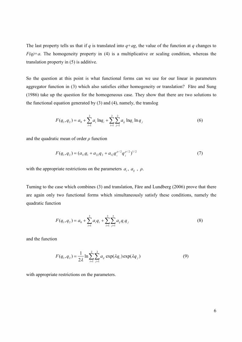
So the question at this point is what functional forms can we use for our linear in parameters

aggregator function in (3) which also satisfies either homogeneity or translation? Färe and Sung

(1986) take up the question for the homogeneous case. They show that there are two solutions to

the functional equation generated by (3) and (4), namely, the translog

j

i

i

j

iji

i

i qqaqaaqqF lnlnln),(2

1

2

1

2

1

021 ∑∑∑= ==

++= (6)

and the quadratic mean of order ρ function

2/12/2/

1222211121 )(),(21

ρρ qqaqaqaqqF ++= (7)

with the appropriate restrictions on the parameters ia , ija , ρ.

Turning to the case which combines (3) and translation, Färe and Lundberg (2006) prove that there

are again only two functional forms which simultaneously satisfy these conditions, namely the

quadratic function

j

i

i

j

iji

i

i qqaqaaqqF ∑∑∑= ==

++=2

1

2

1

2

1

021 ),( (8)

and the function

)exp()exp(ln2

1),(

2

1

2

1

21 j

i

i

j

ij qqaqqF ∑∑= =

= λλλ

(9)

with appropriate restrictions on the parameters.

7

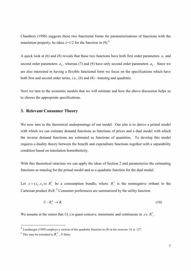
Chambers (1998) suggests these two functional forms for parameterizations of functions with the

translation property; he takes λ=1/2 for the function in (9).4

A quick look at (6) and (8) reveals that these two functions have both first order parameters ia and

second order parameters ija , whereas (7) and (9) have only second order parameters ija . Since we

are also interested in having a flexible functional form we focus on the specifications which have

both first and second order terms, i.e., (6) and (8) - translog and quadratic.

Next we turn to the economic models that we will estimate and how the above discussion helps us

to choose the appropriate specifications.

3. Relevant Consumer Theory

We now turn to the theoretical underpinnings of our model. Our aim is to derive a primal model

with which we can estimate demand functions as functions of prices and a dual model with which

the inverse demand functions are estimated as functions of quantities. To develop this model

requires a duality theory between the benefit and expenditure functions together with a separability

condition based on translation homotheticity.

With this theoretical structure we can apply the ideas of Section 2 and parameterize the estimating

functions as translog for the primal model and as a quadratic function for the dual model.

Let 2

21 ),( +∈= Rxxx be a consumption bundle, where 2

+R is the nonnegative orthant in the

Cartesian product RxR .5 Consumer preferences are summarized by the utility function

.: 2 RRU →+ (10)

We assume at the outset that U(.) is quasi-concave, monotonic and continuous in 2

+∈ Rx .

4 Luenberger (1995) employs a version of the quadratic function in (8) in his exercise 14, p. 127. 5 This may be extended to

NR+ , N finite.

8

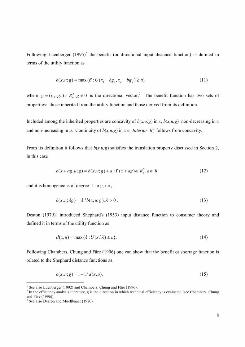
Following Luenberger (1995)6 the benefit (or directional input distance function) is defined in

terms of the utility function as

}),(:max{);,( 2211 ubgxbgxUguxb ≥−−= β (11)

where 0,),( 2

21 ≠∈= + gRggg is the directional vector.7 The benefit function has two sets of

properties: those inherited from the utility function and those derived from its definition.

Included among the inherited properties are concavity of b(x,u;g) in x, b(x,u;g) non-decreasing in x

and non-increasing in u. Continuity of b(x,u;g) in x ∈ Interior 2

+R follows from concavity.

From its definition it follows that b(x,u;g) satisfies the translation property discussed in Section 2,

in this case

aguxbguagxb +=+ );,();,( if RaRagx ∈∈+ + ,)( 2 (12)

and it is homogeneous of degree -1 in g, i.e.,

0),;,();,( 1 >= − λλλ guxbguxb . (13)

Deaton (1979)8 introduced Shephard's (1953) input distance function to consumer theory and

defined it in terms of the utility function as

}.)/(:max{),( uxUuxd ≥= λλ (14)

Following Chambers, Chung and Färe (1996) one can show that the benefit or shortage function is

related to the Shephard distance functions as

),,(/11);,( uxdguxb −= (15)

6 See also Luenberger (1992) and Chambers, Chung and Färe (1996). 7 In the efficiency analysis literature, g is the direction in which technical efficiency is evaluated (see Chambers, Chung and Färe (1996)). 8 See also Deaton and Muellbauer (1980).

9

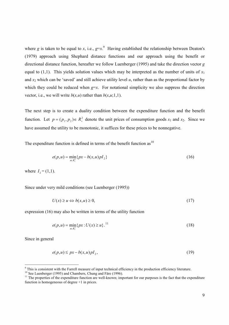
where g is taken to be equal to x, i.e., g=x.9 Having established the relationship between Deaton's

(1979) approach using Shephard distance functions and our approach using the benefit or

directional distance function, hereafter we follow Luenberger (1995) and take the direction vector g

equal to (1,1). This yields solution values which may be interpreted as the number of units of x1

and x2 which can be ‘saved’ and still achieve utility level u, rather than as the proportional factor by

which they could be reduced when g=x. For notational simplicity we also suppress the direction

vector, i.e., we will write b(x,u) rather than b(x,u;1,1).

The next step is to create a duality condition between the expenditure function and the benefit

function. Let 2

21 ),( +∈= Rppp denote the unit prices of consumption goods x1 and x2. Since we

have assumed the utility to be monotonic, it suffices for these prices to be nonnegative.

The expenditure function is defined in terms of the benefit function as10

}),({min),( 22pIuxbpxupe

Rx−=

+∈ (16)

where 2I = (1,1).

Since under very mild conditions (see Luenberger (1995))

,0),()( ≥⇔≥ uxbuxU (17)

expression (16) may also be written in terms of the utility function

}.)(:{min),(2

uxUpxupeRx

≥=+∈

11 (18)

Since in general

,),(),( 2pIuxbpxupe −≤ (19)

9 This is consistent with the Farrell measure of input technical efficiency in the production efficiency literature. 10 See Luenberger (1995) and Chambers, Chung and Färe (1996). 11 The properties of the expenditure function are well-known; important for our purposes is the fact that the expenditure function is homogeneous of degree +1 in prices.

10

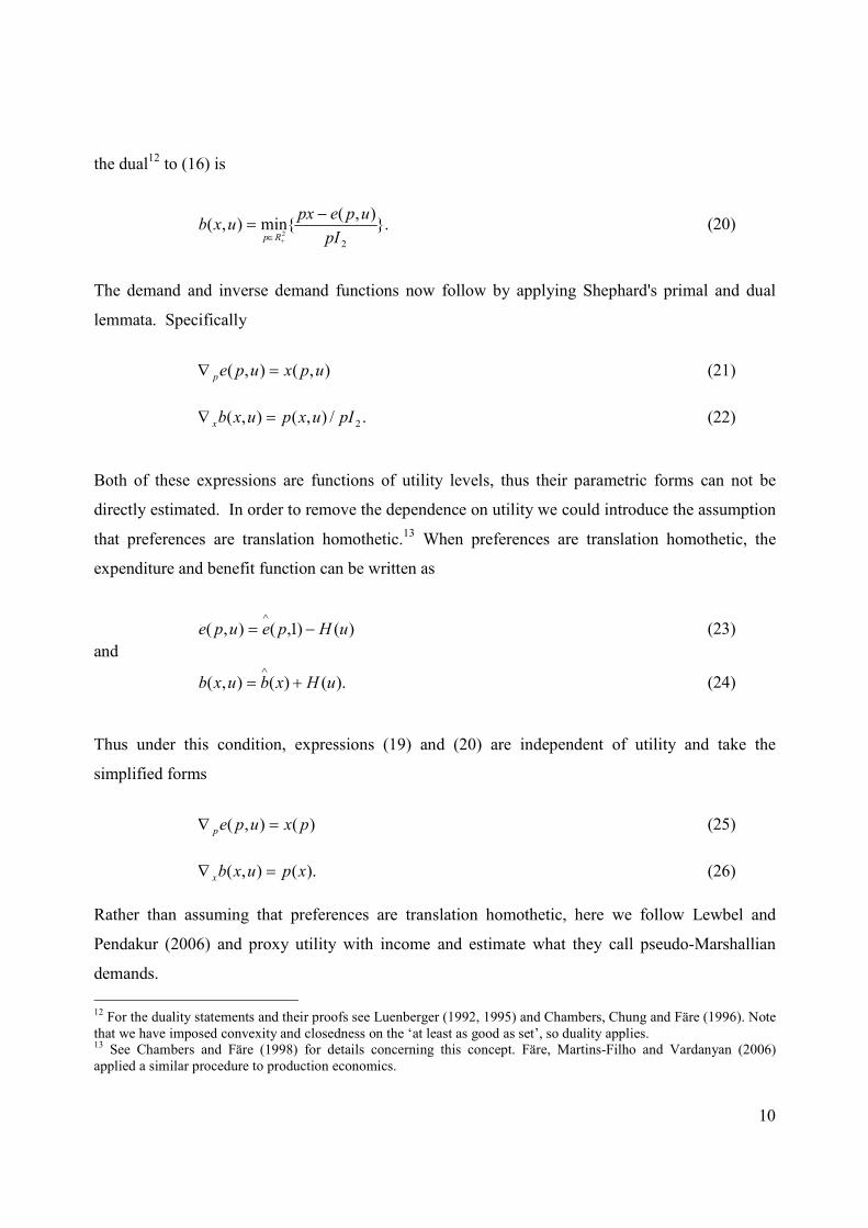
the dual12 to (16) is

}.),(

{min),(2

2 pI

upepxuxb

Rp

−=

+∈ (20)

The demand and inverse demand functions now follow by applying Shephard's primal and dual

lemmata. Specifically

),(),( upxupep =∇ (21)

./),(),( 2pIuxpuxbx =∇ (22)

Both of these expressions are functions of utility levels, thus their parametric forms can not be

directly estimated. In order to remove the dependence on utility we could introduce the assumption

that preferences are translation homothetic.13 When preferences are translation homothetic, the

expenditure and benefit function can be written as

)()1,(),( uHpeupe −=∧

(23)

and

).()(),( uHxbuxb +=∧

(24)

Thus under this condition, expressions (19) and (20) are independent of utility and take the

simplified forms

)(),( pxupep =∇ (25)

).(),( xpuxbx =∇ (26)

Rather than assuming that preferences are translation homothetic, here we follow Lewbel and

Pendakur (2006) and proxy utility with income and estimate what they call pseudo-Marshallian

demands.

12 For the duality statements and their proofs see Luenberger (1992, 1995) and Chambers, Chung and Färe (1996). Note that we have imposed convexity and closedness on the ‘at least as good as set’, so duality applies. 13 See Chambers and Färe (1998) for details concerning this concept. Färe, Martins-Filho and Vardanyan (2006) applied a similar procedure to production economics.

11

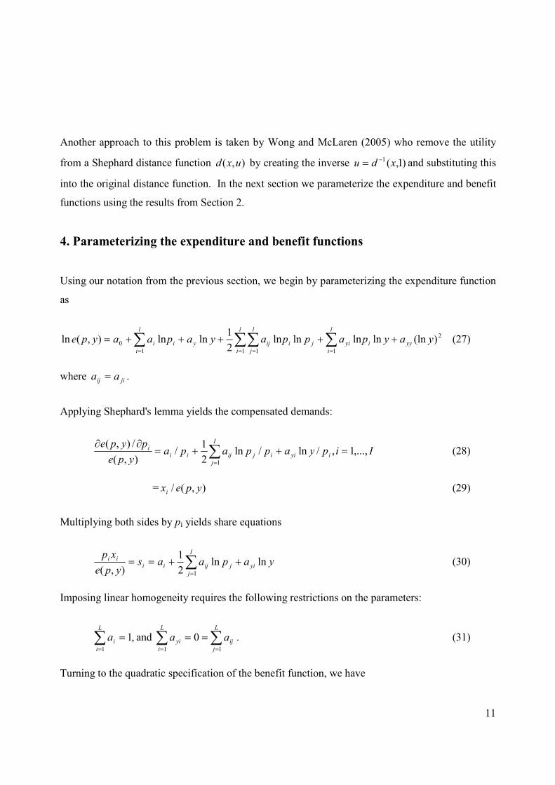
Another approach to this problem is taken by Wong and McLaren (2005) who remove the utility

from a Shephard distance function ),( uxd by creating the inverse )1,(1 xdu −= and substituting this

into the original distance function. In the next section we parameterize the expenditure and benefit

functions using the results from Section 2.

4. Parameterizing the expenditure and benefit functions

Using our notation from the previous section, we begin by parameterizing the expenditure function

as

2

11 11

0 )(lnlnlnlnln2

1lnln),(ln yaypappayapaaype yyi

l

i

yij

l

i

i

l

j

ijyi

l

i

i +++++= ∑∑∑∑== ==

(27)

where jiij aa = .

Applying Shephard's lemma yields the compensated demands:

Iipyappapaype

pypeiyii

I

j

jijii

i ,...,1,/ln/ln2

1/

),(

/),(

1

=++=∂∂

∑=

(28)

= ),(/ ypexi (29)

Multiplying both sides by pi yields share equations

yapaasype

xpyi

I

j

jijii

ii lnln2

1

),( 1

++== ∑=

(30)

Imposing linear homogeneity requires the following restrictions on the parameters:

,11

=∑=

L

i

ia and ∑∑==

==L

j

ij

L

i

yi aa11

0 . (31)

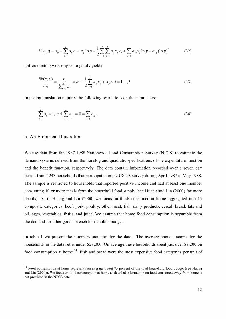
Turning to the quadratic specification of the benefit function, we have

12

2

11 11

0 )(lnln2

1ln),( yayxaxxayaxaayxb yy

l

i

iyij

l

i

i

l

j

ijy

i

l

i

i +++++= ∑∑∑∑== ==

(32)

Differentiating with respect to good i yields

Iiyaxaap

p

x

yxbyi

I

j

jijiL

i i

i

i

,...,1,2

1),(

11

=++==∂

∂∑

∑ ==

(33)

Imposing translation requires the following restrictions on the parameters:

,11

=∑=

L

i

ia and ∑∑==

==L

j

ij

L

i

yi aa11

0 . (34)

5. An Empirical Illustration

We use data from the 1987-1988 Nationwide Food Consumption Survey (NFCS) to estimate the

demand systems derived from the translog and quadratic specifications of the expenditure function

and the benefit function, respectively. The data contain information recorded over a seven day

period from 4243 households that participated in the USDA survey during April 1987 to May 1988.

The sample is restricted to households that reported positive income and had at least one member

consuming 10 or more meals from the household food supply (see Huang and Lin (2000) for more

details). As in Huang and Lin (2000) we focus on foods consumed at home aggregated into 13

composite categories: beef, pork, poultry, other meat, fish, dairy products, cereal, bread, fats and

oil, eggs, vegetables, fruits, and juice. We assume that home food consumption is separable from

the demand for other goods in each household’s budget.

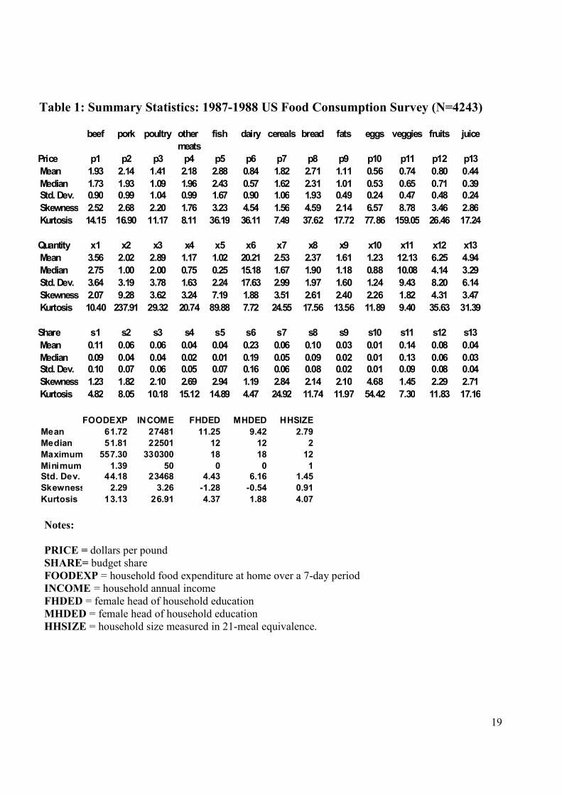
In table 1 we present the summary statistics for the data. The average annual income for the

households in the data set is under $28,000. On average these households spent just over $3,200 on

food consumption at home.14 Fish and bread were the most expensive food categories per unit of

14 Food consumption at home represents on average about 75 percent of the total household food budget (see Huang and Lin (2000)). We focus on food consumption at home as detailed information on food consumed away from home is not provided in the NFCS data.

13

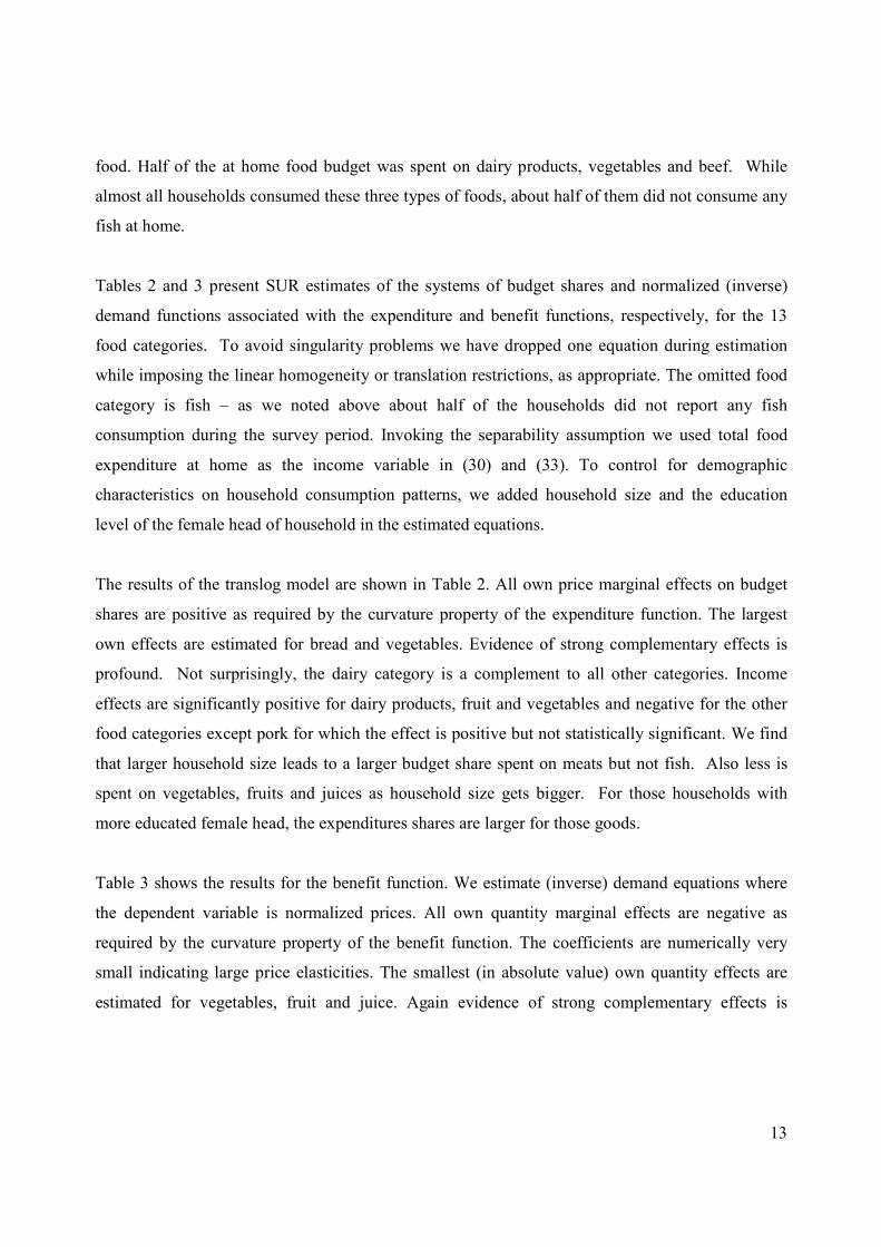
food. Half of the at home food budget was spent on dairy products, vegetables and beef. While

almost all households consumed these three types of foods, about half of them did not consume any

fish at home.

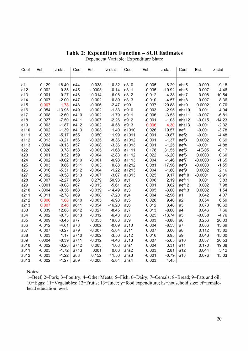
Tables 2 and 3 present SUR estimates of the systems of budget shares and normalized (inverse)

demand functions associated with the expenditure and benefit functions, respectively, for the 13

food categories. To avoid singularity problems we have dropped one equation during estimation

while imposing the linear homogeneity or translation restrictions, as appropriate. The omitted food

category is fish – as we noted above about half of the households did not report any fish

consumption during the survey period. Invoking the separability assumption we used total food

expenditure at home as the income variable in (30) and (33). To control for demographic

characteristics on household consumption patterns, we added household size and the education

level of the female head of household in the estimated equations.

The results of the translog model are shown in Table 2. All own price marginal effects on budget

shares are positive as required by the curvature property of the expenditure function. The largest

own effects are estimated for bread and vegetables. Evidence of strong complementary effects is

profound. Not surprisingly, the dairy category is a complement to all other categories. Income

effects are significantly positive for dairy products, fruit and vegetables and negative for the other

food categories except pork for which the effect is positive but not statistically significant. We find

that larger household size leads to a larger budget share spent on meats but not fish. Also less is

spent on vegetables, fruits and juices as household size gets bigger. For those households with

more educated female head, the expenditures shares are larger for those goods.

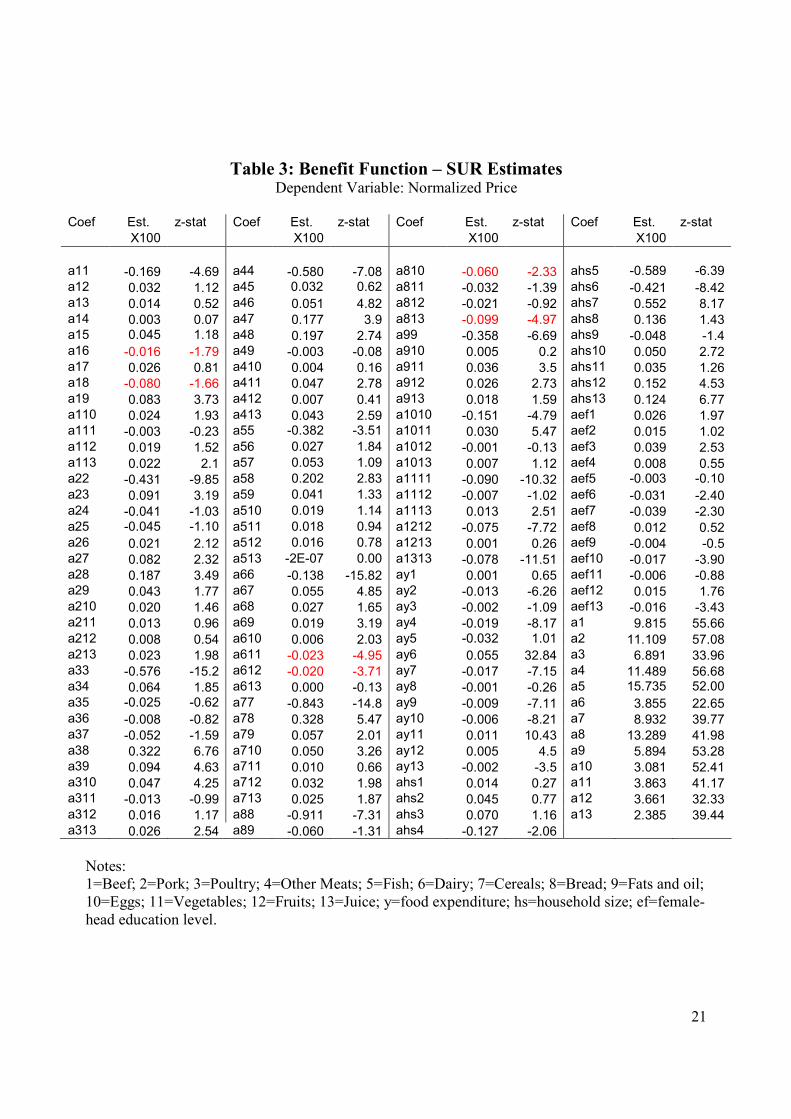
Table 3 shows the results for the benefit function. We estimate (inverse) demand equations where

the dependent variable is normalized prices. All own quantity marginal effects are negative as

required by the curvature property of the benefit function. The coefficients are numerically very

small indicating large price elasticities. The smallest (in absolute value) own quantity effects are

estimated for vegetables, fruit and juice. Again evidence of strong complementary effects is

14

profound albeit not to the extent found in the case of the translog.15 Dairy products appear to be a

substitute for many goods but not for fruits and vegetables. Higher incomes lead to higher prices

paid for dairy products, vegetables and fruit and lower prices for pork, other meats, cereals, fats,

eggs and juice. Household size influences the prices paid for fish and dairy negatively and has a

positive impact on the marginal willingness to pay for cereals, eggs, fruits and juice. More highly

educated female heads are willing to pay more at the margin for poultry but less for dairy products,

cereals, eggs and juice.

A comparison of the empirical results for the translog and quadratic functions gives no prima facie

evidence for choosing one form over the other. Both specifications appear to fit the data quite well

and satisfy the curvature conditions adhered to by consumer theory. However, as reported in table

4, the number of monotonicity violations is much larger for the translog function than the quadratic

function. In fact, it appears that the translog encounters a substantial number of monotonicity

violations for this data set thereby bringing to question the validity of inferences on consumer

behavior.16 We investigate the ability of the two functional forms to satisfy the regularity

conditions of consumer behavior further by conducting a Monte Carlo study.

We follow an experimental design similar to that used in the Monte Carlo study by Barnett and

Usui (2006). The following procedure is adopted: (1) a vector of prices is created based on

observed data plus an error term generated from a multivatiate normal with mean zero and

covariance matrix equal to a multiple, ∈µ [0,1] , of the actual price covariance matrix while

ensuring that prices remain nonnegative; (2) we feed the price data along with total expenditure (y)

to demand equations derived from a CES indirect utility function to generate data on quantities

demanded; (3) we use the price, quantity and income data to estimate the budget share and

normalized price equations derived from the translog and quadratic function specifications of the

expenditure function and benefit function, respectively.

15 Note that valuations of complementary relationships across different types of foods may be of interest for welfare analysis purposes – e.g. enhance the effectiveness of government food programs. 16 Basmann, Molina and Slottje (1983) have drawn attention to the inference problem that arises in the estimation of consumer demand systems when regularity conditions are violated. See also Barnett and Usui (2006).

15

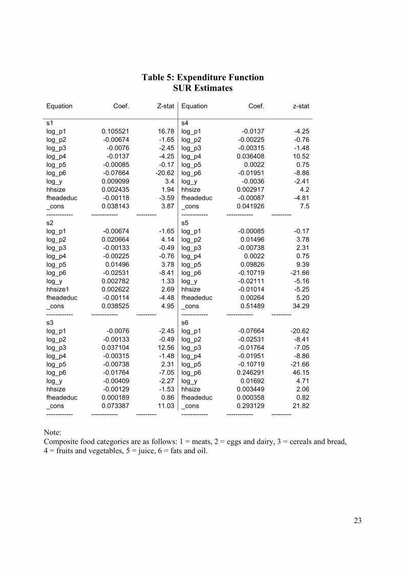
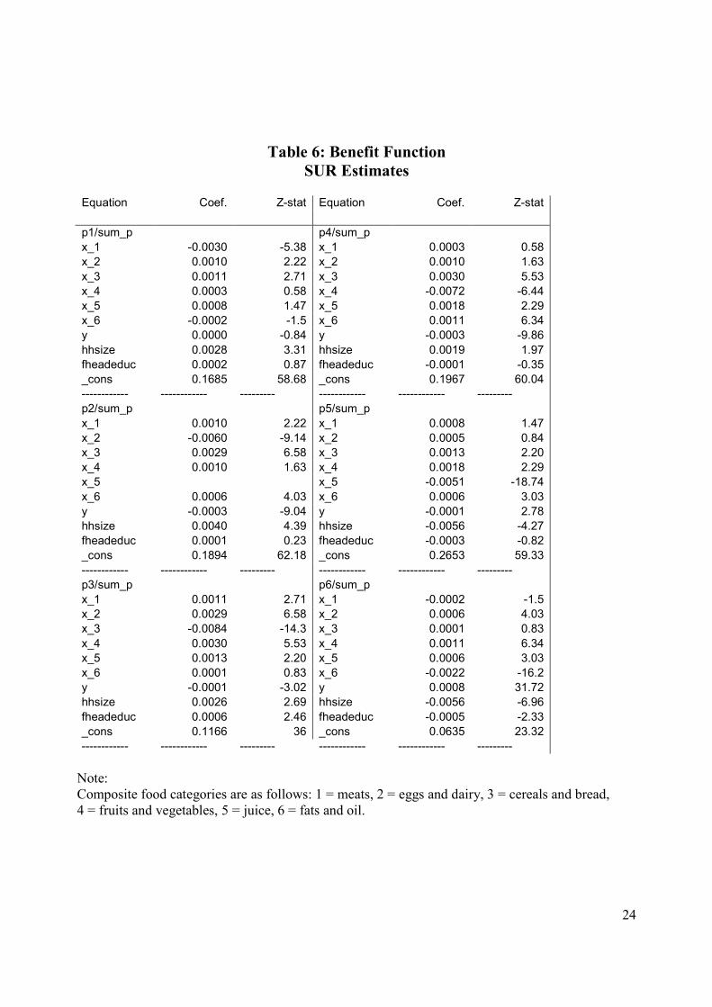
We assess the two functional forms by estimating systems of demand equations for six composite

food categories: meats, eggs and dairy, cereals and bread, fruits and vegetables, juice, fats and oil.17

The CES indirect utility function with six goods is given by:

r

i

r

ipyypV

/16

1

),(

−

=

= ∑ where )1/( −= ρρr , 1≤ρ

Using Roy’s identity to the CES indirect utility function, we can derive Marshallian demand

functions (see Barnett and Usui (2006)) as:

∑=

−=6

1

1 /),(j

r

j

r

ii pypypq

Quantities are generated based on the generated prices for given income and values of ρ . We

choose values of ρ that give rise to a sufficiently wide range of elasticities of substitution, defined

as )1/(1 ρσ −= . Using the simulated price and quantity data, we calculate the expenditures shares

and normalized prices required to estimate the systems of equations given in (30) and (33) above.

The number of Monte Carlo replications is 1000 so we estimate the two equations 1000 times and

check for regularity violations in each case. We repeat the same experiment using values of σ

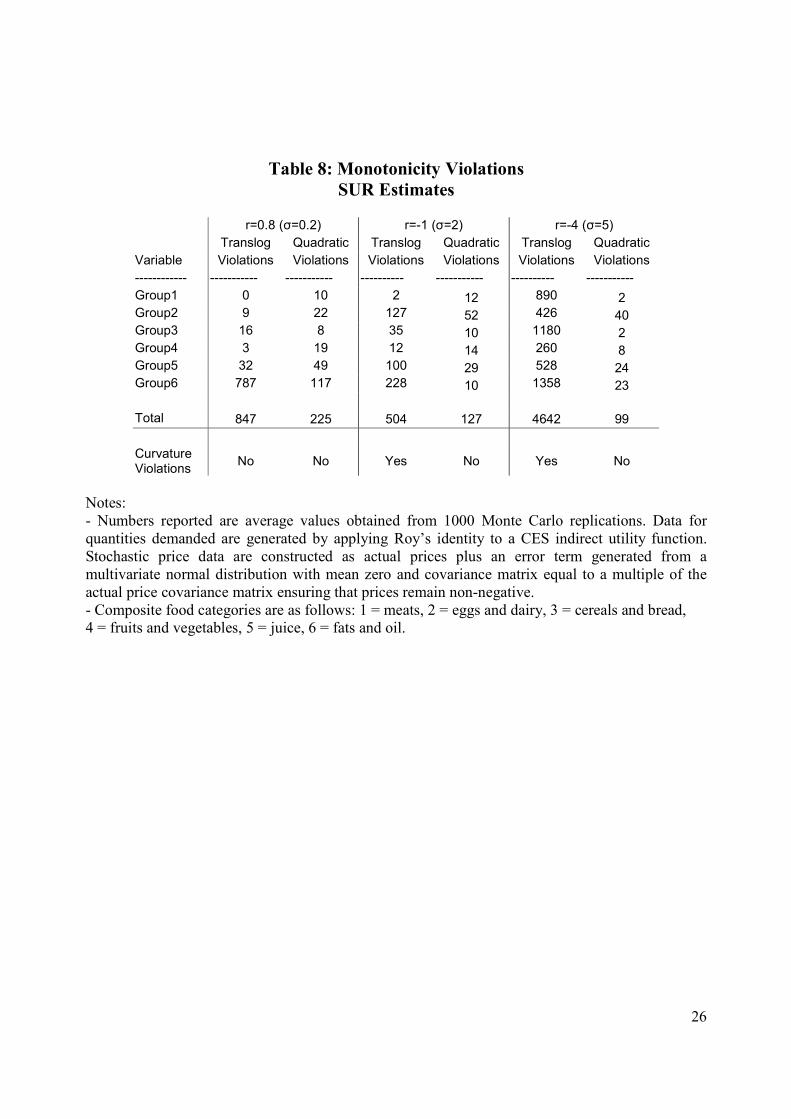
ranging from 0.2 to 8. In table 8, we report regularity violations for elasticitity of substitution

values set to 0.2, 2 and 5. While both functional forms satisfy the curvature condition when the data

is generated with elasticities of substitution less than one, the translog fails to produce meaningful

results for values of σ >1. In all cases we find that the quadratic encounters far less monotonicity

violations than the translog.18

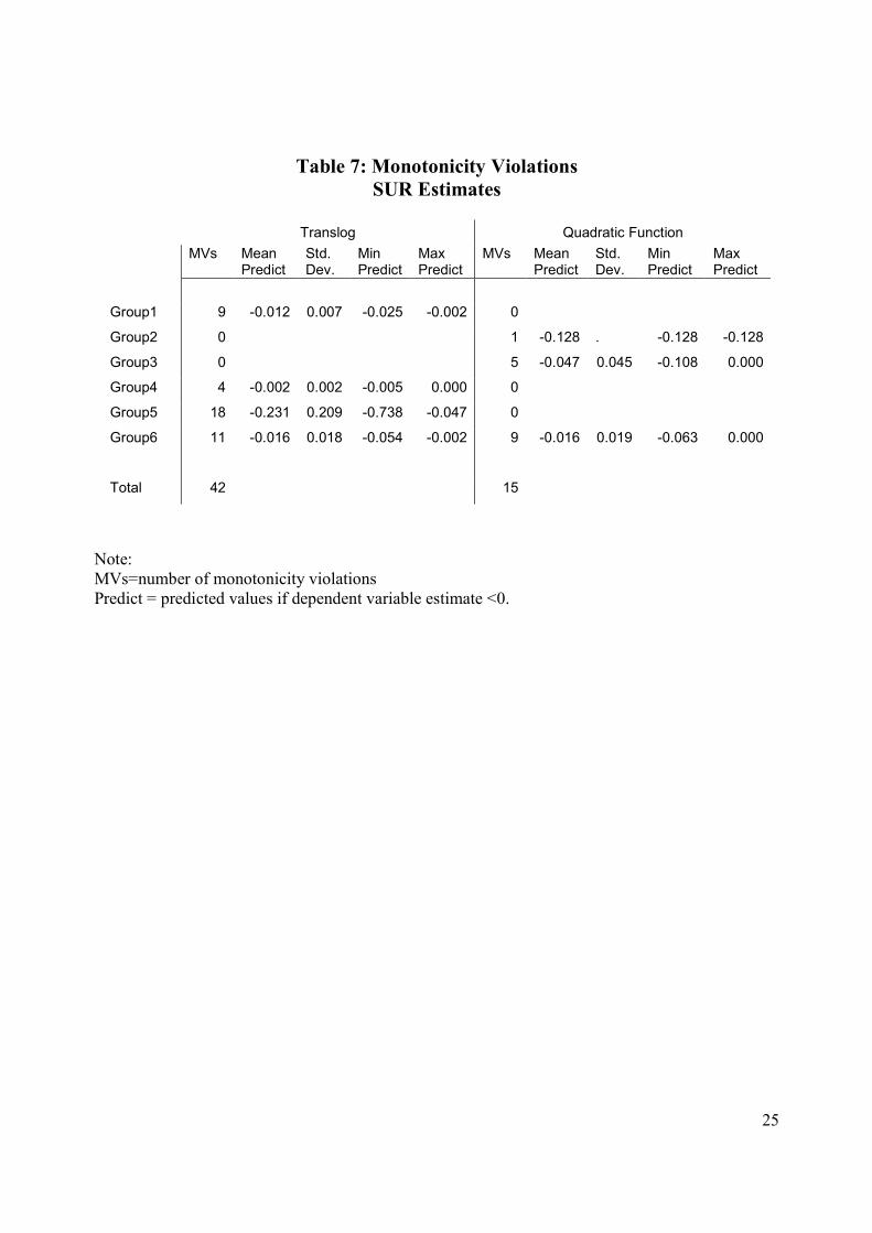
17 SUR estimates of the budget shares and normalized prices equations using observed data for the six composite goods categories are reported in Tables 5 and 6, respectively. Both functions satisfy the curvature conditions. Monotonicity violations are reported in Table 7. 18 While not reported here, we experimented further using the Diewert reciprocal indirect utility function (with homothetic preferences) and the translog reciprocal indirect utility function to generate quantity data. Again, the evidence indicates that the quadratic specification performs better than the translog model.

16

References Aczél, J. (1966), Functional Equations and their Applications, Academic Press: New York. Banks, J., R. Blundell and A. Lewbel. (1997) "Quadratic Engel Curves and Consumer Demand" Review of Economics and Statistics 79 ( 4), 527-539. Barnett, W. A. and S. Choi. (1989) "A Monte Carlo Study of Tests of Blockwise Weak Separability" Journal of Business and Economic Statistics 7 (3), 363-377. Barnett, William A., and Yul W. Lee. (1985) "The Global Properties of the Miniflex Laurent, Generalized Leontief, and Translog Flexible Functional Forms" Econometrica 53 (6), 1421-1437. Barnett, W., and I. Usui. (2006) "The Theoretical Regularity Properties of the Normalized Quadratic Consumer Demand Model" University of Kansas, Department of Economics, Working Papers Series in Theoretical and Applied Economics: 200609. Barten, A. P., and L. J. Bettendorf. (1989) "Price Formation of Fish: An Application of an Inverse Demand System" European Economic Review 33 (8), 1509-1525. Basmann, R. L., D.J. Molina and D.J. Slottje (1983), “Budget Constraint Prices as Preference Changing Parameters of Generalized Fechner-Thurstone Direct Utility Functions” American

Economic Review 73 (3), 411-413, Berndt, E., R., Darrough, N. Masako and W. E. Diewert. (1977) "Flexible Functional Forms and Expenditure Distributions: An Application to Canadian Consumer Demand Functions" International Economic Review 18 (3), 651-675. Caves, D. W., and L. R. Christensen. (1980) "Global Properties of Flexible Functional Forms" American Economic Review 70 (3), 422-432. Chambers, R. G. (1988), Applied Production Analysis: A dual approach, Cambridge University Press: Cambridge. Chambers, R. G. (1998), Input and Output Indicators” in Index Numbers: Essays in Honour of Sten

Malmquist, R. Färe, S. Grosskopf and R.R Russell (eds.), Kluwer: Boston. Chambers, R. G. (2002), “Exact Nonradial Input, Output, and Productivity Measurement” Economic Theory 20, 751-765. Chambers, R. G., Y. Chung and R. Färe (1996), “Benefit and Distance Functions" Journal of Economic Theory 70(2) (August), 407-419. Christensen, L.R., D.W. Jorgenson and L.J. Lau. (1975) "Transcendental Logarithmic Utility Functions" American Economic Review 65 (3), 367-383.

17

Deaton, A. (1979), “The Distance Function and Consumer Behaviour with Applications to Index Numbers and Optimal Taxation” Review of Economic Studies 46, 391-405. Deaton, A. and J. Muellbauer (1980), Economics and Consumer Behaviour, Cambridge University Press: Cambridge. Diewert, E.W. (1971), “An Application of the Shephard Duality Theorem: A Generalized Leontief Production Function” Journal of Political Economy 79, 481-507. Diewert, E.W. (1976), “Exact and Superlative Index Numbers” Journal of Econometrics 4, 116-145. Diewert, E.W. (2002), “The Quadratic Approximation Lemma and Decompositions of the Superlatoive Indexes” Journal of Economic and Social Measurement 28, 63-88. Eales, J. S., and L. J. Unnevehr. (1994) "The Inverse Almost Ideal Demand System" European Economic Review 38 (1), 101-115. Färe, R. and S. Grosskopf. (2000), “Theory and Application of Directional Distance Functions" Journal of Productivity Analysis 13(2) (March), 93-103. Färe, R. and S. Grosskopf (2004), New Directions: Efficiency and Productivity, Kluwer Academic Publishers: Boston. Färe, R. and A. Lundberg (2006), “Parameterizing the Shortage Function" mimeo, Department of Economics, Oregon State University. Färe, R., C. Martins-Filho and M. Vardanyan (2006), “On Functional Form Representation of Multi-Output Production Technologies" mimeo, Department of Economics, Oregon State University. Färe, R. and D. Primont (1995), Multi-Output Production and Duality: Theory and Applications, Kluwer Academic Publishers: Boston. Färe, R.and K. Sung (1986) “On Second-Order Taylor's-Series Approximation and Linear Homogeneity” Aequationes Mathematicae 30, 180-186. Fisher, D., A.R. Fleissig and A. Serletis (2001) "An Empirical Comparison of Flexible Demand System Functional Forms" Journal of Applied Econometrics 16 (1), 59-80. Holt, M. T., and R. C. Bishop (2002) "A Semiflexible Normalized Quadratic Inverse Demand System: An Application to the Price Formation of Fish." Empirical Economics 27 (1), 23-47. Huang, Kuo S. and Biing-Hwan Lin(2000), “Estimation of Food Demand and Nutrient Elasticities from Household Survey Data. Rood and Rural Economics Division, Economic Research Service, U.S. Department of Agriculture. Technical Bulletin No. 1887.

18

Lewbel, A. and K. Pendakur (2006), “Tricks with Hicks: The EASI Demand System" mimeo. Luenberger, D. G. (1992), “Benefit Functions and Duality” Journal of Mathematical Economics 21, 461-481. Luenberger, D. G. (1995), Microeconomic Theory, McGraw-Hill: New York. Moschini, G. (1998) "The Semiflexible Almost Ideal Demand System." European Economic

Review 42 (2), 349-364. Moschini, G. and A. Vissa. 1992. "A Linear Inverse Demand System." Journal of Agricultural and Resource Economics 17 (2), 294-302. Pollak, R. A. and T. J. Wales (1978), “Estimation of Complete Demand Systems from Household Budget Data: the Linear and Quadratic Expenditure Systems" American Economic Review 68:3, 348-359. Shephard, R. W. (1953), Cost and Production Functions, Princeton: Princeton University Press. Shephard, R. W. (1970), Theory of Cost and Production Functions, Princeton: Princeton University Press. Thiel, Henri. (1975) The Theory of Measurement of Consumer Demand: Volume I, Amsterdam: North-Holland Publishing Co. Thiel, Henri. (1976) The Theory of Measurement of Consumer Demand: VolumeII, Amsterdam: North-Holland Publishing Co. Wong, K.K.G. and K. R. McLaren (2005), “Specification and Estimation of Regular Inverse Demand Systems: a Distance Function Approach" American Journal of Agricultural Economics 87 (4), 823-834.

19

Table 1: Summary Statistics: 1987-1988 US Food Consumption Survey (N=4243)

beef pork poultry other fish dairy cereals bread fats eggs veggies fruits juice

meats

Price p1 p2 p3 p4 p5 p6 p7 p8 p9 p10 p11 p12 p13

Mean 1.93 2.14 1.41 2.18 2.88 0.84 1.82 2.71 1.11 0.56 0.74 0.80 0.44

Median 1.73 1.93 1.09 1.96 2.43 0.57 1.62 2.31 1.01 0.53 0.65 0.71 0.39

Std. Dev. 0.90 0.99 1.04 0.99 1.67 0.90 1.06 1.93 0.49 0.24 0.47 0.48 0.24

Skewness 2.52 2.68 2.20 1.76 3.23 4.54 1.56 4.59 2.14 6.57 8.78 3.46 2.86

Kurtosis 14.15 16.90 11.17 8.11 36.19 36.11 7.49 37.62 17.72 77.86 159.05 26.46 17.24

Quantity x1 x2 x3 x4 x5 x6 x7 x8 x9 x10 x11 x12 x13

Mean 3.56 2.02 2.89 1.17 1.02 20.21 2.53 2.37 1.61 1.23 12.13 6.25 4.94

Median 2.75 1.00 2.00 0.75 0.25 15.18 1.67 1.90 1.18 0.88 10.08 4.14 3.29

Std. Dev. 3.64 3.19 3.78 1.63 2.24 17.63 2.99 1.97 1.60 1.24 9.43 8.20 6.14

Skewness 2.07 9.28 3.62 3.24 7.19 1.88 3.51 2.61 2.40 2.26 1.82 4.31 3.47

Kurtosis 10.40 237.91 29.32 20.74 89.88 7.72 24.55 17.56 13.56 11.89 9.40 35.63 31.39

Share s1 s2 s3 s4 s5 s6 s7 s8 s9 s10 s11 s12 s13

Mean 0.11 0.06 0.06 0.04 0.04 0.23 0.06 0.10 0.03 0.01 0.14 0.08 0.04

Median 0.09 0.04 0.04 0.02 0.01 0.19 0.05 0.09 0.02 0.01 0.13 0.06 0.03

Std. Dev. 0.10 0.07 0.06 0.05 0.07 0.16 0.06 0.08 0.02 0.01 0.09 0.08 0.04

Skewness 1.23 1.82 2.10 2.69 2.94 1.19 2.84 2.14 2.10 4.68 1.45 2.29 2.71

Kurtosis 4.82 8.05 10.18 15.12 14.89 4.47 24.92 11.74 11.97 54.42 7.30 11.83 17.16

FOODEXP INCOME FHDED MHDED HHSIZE

Mean 61.72 27481 11.25 9.42 2.79

Median 51.81 22501 12 12 2

Maximum 557.30 330300 18 18 12

Minimum 1.39 50 0 0 1

Std. Dev. 44.18 23468 4.43 6.16 1.45

Skewness 2.29 3.26 -1.28 -0.54 0.91

Kurtosis 13.13 26.91 4.37 1.88 4.07

Notes:

PRICE = dollars per pound SHARE= budget share FOODEXP = household food expenditure at home over a 7-day period INCOME = household annual income FHDED = female head of household education MHDED = female head of household education HHSIZE = household size measured in 21-meal equivalence.

20

Table 2: Expenditure Function – SUR Estimates Dependent Variable: Expenditure Share

Coef Est. z-stat Coef Est. z-stat Coef Est. z-stat Coef Est. z-stat

a11 0.129 18.49 a44 0.038 10.32 a810 -0.005 -6.29 ahs5 -0.009 -9.18

a12 0.002 0.35 a45 -.0003 -0.14 a811 -0.035 -10.92 ahs6 0.007 4.46

a13 -0.001 -0.27 a46 -0.014 -6.08 a812 -0.012 -4.38 ahs7 0.008 10.54

a14 -0.007 -2.00 a47 0.002 0.89 a813 -0.010 -4.57 ahs8 0.007 8.36

a15 0.007 1.78 a48 -0.006 -2.47 a99 0.037 20.88 ahs9 0.0002 0.70

a16 -0.054 -13.95 a49 -0.002 -1.33 a910 -0.003 -2.95 ahs10 0.001 4.04

a17 -0.008 -2.60 a410 -0.002 -1.79 a911 -0.006 -3.53 ahs11 -0.007 -6.81

a18 -0.027 -7.50 a411 -0.007 -2.26 a912 -0.001 -1.03 ahs12 -0.015 -14.23

a19 -0.003 -1.87 a412 -0.002 -0.58 a913 0.006 4.30 ahs13 -0.001 -2.32

a110 -0.002 -1.39 a413 0.003 1.40 a1010 0.026 19.57 aef1 -0.001 -3.78

a111 -0.023 -5.17 a55 0.050 11.99 a1011 -0.001 -0.87 aef2 -0.001 -4.48

a112 -0.013 -3.21 a56 -0.025 -8.36 a1012 -0.001 -1.37 aef3 0.0002 0.69

a113 -.0004 -0.13 a57 -0.008 -3.36 a1013 -0.001 -1.25 aef4 -0.001 -4.88

a22 0.020 3.78 a58 -0.005 -1.68 a1111 0.178 31.55 aef5 -4E-05 -0.17

a23 0.001 0.52 a59 -0.004 -2.83 a1112 -0.022 -6.20 aef6 0.0003 0.60

a24 -0.002 -0.62 a510 -0.001 -0.98 a1113 -0.004 -1.46 aef7 -0.0003 -1.65

a25 0.003 0.86 a511 0.003 0.88 a1212 0.081 17.96 aef8 -0.0003 -1.55

a26 -0.016 -5.31 a512 -0.004 -1.22 a1213 -0.004 -1.80 aef9 0.0002 2.16

a27 -0.002 -0.58 a513 -0.007 -3.07 a1313 0.025 9.17 aef10 -0.0001 -2.91

a28 -0.007 -2.27 a66 0.279 50.93 ay1 0.006 2.19 aef11 0.001 3.83

a29 -.0001 -0.08 a67 -0.013 -5.61 ay2 0.001 0.62 aef12 0.002 7.98

a210 -.0004 -0.36 a68 -0.039 -14.49 ay3 -0.005 -3.00 aef13 0.0002 1.54

a211 -0.011 -2.78 a69 -0.008 -7.20 ay4 -0.004 -2.96 a1 0.042 4.07

a212 0.006 1.68 a610 -0.005 -6.98 ay5 0.020 9.40 a2 0.054 6.59

a213 0.007 2.46 a611 -0.054 -16.20 ay6 0.012 3.48 a3 0.073 10.62

a33 0.039 12.88 a612 -0.027 -8.45 ay7 -0.013 -8.00 a4 0.046 7.66

a34 -0.002 -0.73 a613 -0.012 -6.43 ay8 -0.025 -13.74 a5 -0.038 -4.76

a35 -0.009 -3.45 a77 0.055 19.83 ay9 -0.003 -3.88 a6 0.256 20.03

a36 -0.012 -4.61 a78 -.0002 -0.09 ay10 -0.004 -8.53 a7 0.086 13.69

a37 -0.007 -3.27 a79 -0.007 -5.84 ay11 0.007 3.00 a8 0.112 15.82

a38 0.003 1.17 a710 -0.002 -3.50 ay12 0.016 6.95 a9 0.043 15.00

a39 -.0004 -0.39 a711 -0.012 -4.46 ay13 -0.007 -5.65 a10 0.037 20.53

a310 -0.002 -3.28 a712 0.003 1.08 ahs1 0.004 3.31 a11 0.170 19.38

a311 -0.005 -1.72 a713 .0001 0.03 ahs2 0.003 2.81 a12 0.044 5.12

a312 -0.003 -1.22 a88 0.152 41.50 ahs3 -0.001 -0.79 a13 0.076 15.03

a313 -0.002 -1.27 a89 -0.008 -5.84 ahs4 0.003 4.45

Notes: 1=Beef; 2=Pork; 3=Poultry; 4=Other Meats; 5=Fish; 6=Dairy; 7=Cereals; 8=Bread; 9=Fats and oil; 10=Eggs; 11=Vegetables; 12=Fruits; 13=Juice; y=food expenditure; hs=household size; ef=female-head education level.

21

Table 3: Benefit Function – SUR Estimates Dependent Variable: Normalized Price

Coef Est. z-stat Coef Est. z-stat Coef Est. z-stat Coef Est. z-stat

X100 X100 X100 X100

a11 -0.169 -4.69 a44 -0.580 -7.08 a810 -0.060 -2.33 ahs5 -0.589 -6.39

a12 0.032 1.12 a45 0.032 0.62 a811 -0.032 -1.39 ahs6 -0.421 -8.42 a13 0.014 0.52 a46 0.051 4.82 a812 -0.021 -0.92 ahs7 0.552 8.17 a14 0.003 0.07 a47 0.177 3.9 a813 -0.099 -4.97 ahs8 0.136 1.43 a15 0.045 1.18 a48 0.197 2.74 a99 -0.358 -6.69 ahs9 -0.048 -1.4 a16 -0.016 -1.79 a49 -0.003 -0.08 a910 0.005 0.2 ahs10 0.050 2.72 a17 0.026 0.81 a410 0.004 0.16 a911 0.036 3.5 ahs11 0.035 1.26 a18 -0.080 -1.66 a411 0.047 2.78 a912 0.026 2.73 ahs12 0.152 4.53 a19 0.083 3.73 a412 0.007 0.41 a913 0.018 1.59 ahs13 0.124 6.77 a110 0.024 1.93 a413 0.043 2.59 a1010 -0.151 -4.79 aef1 0.026 1.97 a111 -0.003 -0.23 a55 -0.382 -3.51 a1011 0.030 5.47 aef2 0.015 1.02 a112 0.019 1.52 a56 0.027 1.84 a1012 -0.001 -0.13 aef3 0.039 2.53 a113 0.022 2.1 a57 0.053 1.09 a1013 0.007 1.12 aef4 0.008 0.55 a22 -0.431 -9.85 a58 0.202 2.83 a1111 -0.090 -10.32 aef5 -0.003 -0.10

a23 0.091 3.19 a59 0.041 1.33 a1112 -0.007 -1.02 aef6 -0.031 -2.40 a24 -0.041 -1.03 a510 0.019 1.14 a1113 0.013 2.51 aef7 -0.039 -2.30 a25 -0.045 -1.10 a511 0.018 0.94 a1212 -0.075 -7.72 aef8 0.012 0.52 a26 0.021 2.12 a512 0.016 0.78 a1213 0.001 0.26 aef9 -0.004 -0.5 a27 0.082 2.32 a513 -2E-07 0.00 a1313 -0.078 -11.51 aef10 -0.017 -3.90 a28 0.187 3.49 a66 -0.138 -15.82 ay1 0.001 0.65 aef11 -0.006 -0.88 a29 0.043 1.77 a67 0.055 4.85 ay2 -0.013 -6.26 aef12 0.015 1.76 a210 0.020 1.46 a68 0.027 1.65 ay3 -0.002 -1.09 aef13 -0.016 -3.43 a211 0.013 0.96 a69 0.019 3.19 ay4 -0.019 -8.17 a1 9.815 55.66 a212 0.008 0.54 a610 0.006 2.03 ay5 -0.032 1.01 a2 11.109 57.08 a213 0.023 1.98 a611 -0.023 -4.95 ay6 0.055 32.84 a3 6.891 33.96 a33 -0.576 -15.2 a612 -0.020 -3.71 ay7 -0.017 -7.15 a4 11.489 56.68 a34 0.064 1.85 a613 0.000 -0.13 ay8 -0.001 -0.26 a5 15.735 52.00

a35 -0.025 -0.62 a77 -0.843 -14.8 ay9 -0.009 -7.11 a6 3.855 22.65 a36 -0.008 -0.82 a78 0.328 5.47 ay10 -0.006 -8.21 a7 8.932 39.77 a37 -0.052 -1.59 a79 0.057 2.01 ay11 0.011 10.43 a8 13.289 41.98 a38 0.322 6.76 a710 0.050 3.26 ay12 0.005 4.5 a9 5.894 53.28 a39 0.094 4.63 a711 0.010 0.66 ay13 -0.002 -3.5 a10 3.081 52.41 a310 0.047 4.25 a712 0.032 1.98 ahs1 0.014 0.27 a11 3.863 41.17 a311 -0.013 -0.99 a713 0.025 1.87 ahs2 0.045 0.77 a12 3.661 32.33 a312 0.016 1.17 a88 -0.911 -7.31 ahs3 0.070 1.16 a13 2.385 39.44 a313 0.026 2.54 a89 -0.060 -1.31 ahs4 -0.127 -2.06

Notes: 1=Beef; 2=Pork; 3=Poultry; 4=Other Meats; 5=Fish; 6=Dairy; 7=Cereals; 8=Bread; 9=Fats and oil; 10=Eggs; 11=Vegetables; 12=Fruits; 13=Juice; y=food expenditure; hs=household size; ef=female-head education level.

22

Table 4: Monotonicity Violations SUR Estimates

Note: MVs=number of monotonicity violations Predict = predicted values if dependent variable estimate <0.

Translog Quadratic Function

Variable MVs Mean Predict

Std. Dev.

Min Predict

Max Predict

MVs Mean Predict

Std. Dev.

Min Predict

Max Predict

Beef 4 -0.0096 0.0076 -0.0182 -0.0029 0

Pork 0 1 -0.0998 . -0.0998 -0.0998

Poultry 0 7 -0.0293 0.0259 -0.0704 -0.0046

Other 3 -0.0006 0.0004 -0.0011 -0.0003 0

Fish 59 -0.0147 0.0135 -0.0539 -0.0002 1 -0.0146 . -0.0146 -0.0146

Dairy 9 -0.0256 0.0146 -0.0434 -0.0038 14 -0.0092 0.0104 -0.0397 -0.0005

Cereals 20 -0.0092 0.0080 -0.0250 0.0000 4 -0.0123 0.0039 -0.0163 -0.0080

Bread 27 -0.0149 0.0201 -0.0999 -0.0002 0

Fats 6 -0.0050 0.0039 -0.0100 -0.0002 0

Eggs 58 -0.0024 0.0023 -0.0103 0.0000 0

Veggies 6 -0.0232 0.0173 -0.0432 -0.0045 0

Fruits 28 -0.0152 0.0156 -0.0552 0.0000 0

Juice 4 -0.0020 0.0016 -0.0035 -0.0001 1 -0.0153 . -0.0153 -0.0153

Total 224 28

23

Table 5: Expenditure Function

SUR Estimates Equation Coef. Z-stat Equation Coef. z-stat

s1 s4

log_p1 0.105521 16.78 log_p1 -0.0137 -4.25

log_p2 -0.00674 -1.65 log_p2 -0.00225 -0.76

log_p3 -0.0076 -2.45 log_p3 -0.00315 -1.48

log_p4 -0.0137 -4.25 log_p4 0.036408 10.52

log_p5 -0.00085 -0.17 log_p5 0.0022 0.75

log_p6 -0.07664 -20.62 log_p6 -0.01951 -8.86

log_y 0.009099 3.4 log_y -0.0036 -2.41

hhsize 0.002435 1.94 hhsize 0.002917 4.2

fheadeduc -0.00118 -3.59 fheadeduc -0.00087 -4.81

_cons 0.038143 3.87 _cons 0.041926 7.5

------------ ------------ --------- ------------ ------------ ---------

s2 s5

log_p1 -0.00674 -1.65 log_p1 -0.00085 -0.17

log_p2 0.020664 4.14 log_p2 0.01496 3.78

log_p3 -0.00133 -0.49 log_p3 -0.00738 2.31

log_p4 -0.00225 -0.76 log_p4 0.0022 0.75

log_p5 0.01496 3.78 log_p5 0.09826 9.39

log_p6 -0.02531 -8.41 log_p6 -0.10719 -21.66

log_y 0.002782 1.33 log_y -0.02111 -5.16

hhsize1 0.002622 2.69 hhsize -0.01014 -5.25

fheadeduc -0.00114 -4.48 fheadeduc 0.00264 5.20

_cons 0.038525 4.95 _cons 0.51489 34.29

------------ ------------ --------- ------------ ------------ ---------

s3 s6

log_p1 -0.0076 -2.45 log_p1 -0.07664 -20.62

log_p2 -0.00133 -0.49 log_p2 -0.02531 -8.41

log_p3 0.037104 12.56 log_p3 -0.01764 -7.05

log_p4 -0.00315 -1.48 log_p4 -0.01951 -8.86

log_p5 -0.00738 2.31 log_p5 -0.10719 -21.66

log_p6 -0.01764 -7.05 log_p6 0.246291 46.15

log_y -0.00409 -2.27 log_y 0.01692 4.71

hhsize -0.00129 -1.53 hhsize 0.003449 2.06

fheadeduc 0.000189 0.86 fheadeduc 0.000358 0.82

_cons 0.073387 11.03 _cons 0.293129 21.82

------------ ------------ --------- ------------ ------------ ---------

Note: Composite food categories are as follows: 1 = meats, 2 = eggs and dairy, 3 = cereals and bread, 4 = fruits and vegetables, 5 = juice, 6 = fats and oil.

24

Table 6: Benefit Function

SUR Estimates Equation Coef. Z-stat Equation Coef. Z-stat

p1/sum_p p4/sum_p

x_1 -0.0030 -5.38 x_1 0.0003 0.58

x_2 0.0010 2.22 x_2 0.0010 1.63

x_3 0.0011 2.71 x_3 0.0030 5.53

x_4 0.0003 0.58 x_4 -0.0072 -6.44

x_5 0.0008 1.47 x_5 0.0018 2.29

x_6 -0.0002 -1.5 x_6 0.0011 6.34

y 0.0000 -0.84 y -0.0003 -9.86

hhsize 0.0028 3.31 hhsize 0.0019 1.97

fheadeduc 0.0002 0.87 fheadeduc -0.0001 -0.35

_cons 0.1685 58.68 _cons 0.1967 60.04

------------ ------------ --------- ------------ ------------ ---------

p2/sum_p p5/sum_p

x_1 0.0010 2.22 x_1 0.0008 1.47

x_2 -0.0060 -9.14 x_2 0.0005 0.84

x_3 0.0029 6.58 x_3 0.0013 2.20

x_4 0.0010 1.63 x_4 0.0018 2.29

x_5 x_5 -0.0051 -18.74

x_6 0.0006 4.03 x_6 0.0006 3.03

y -0.0003 -9.04 y -0.0001 2.78

hhsize 0.0040 4.39 hhsize -0.0056 -4.27

fheadeduc 0.0001 0.23 fheadeduc -0.0003 -0.82

_cons 0.1894 62.18 _cons 0.2653 59.33

------------ ------------ --------- ------------ ------------ ---------

p3/sum_p p6/sum_p

x_1 0.0011 2.71 x_1 -0.0002 -1.5

x_2 0.0029 6.58 x_2 0.0006 4.03

x_3 -0.0084 -14.3 x_3 0.0001 0.83

x_4 0.0030 5.53 x_4 0.0011 6.34

x_5 0.0013 2.20 x_5 0.0006 3.03

x_6 0.0001 0.83 x_6 -0.0022 -16.2

y -0.0001 -3.02 y 0.0008 31.72

hhsize 0.0026 2.69 hhsize -0.0056 -6.96

fheadeduc 0.0006 2.46 fheadeduc -0.0005 -2.33

_cons 0.1166 36 _cons 0.0635 23.32

------------ ------------ --------- ------------ ------------ ---------

Note: Composite food categories are as follows: 1 = meats, 2 = eggs and dairy, 3 = cereals and bread, 4 = fruits and vegetables, 5 = juice, 6 = fats and oil.

25

Table 7: Monotonicity Violations

SUR Estimates

Translog Quadratic Function

MVs Mean Predict

Std. Dev.

Min Predict

Max Predict

MVs Mean Predict

Std. Dev.

Min Predict

Max Predict

Group1 9 -0.012 0.007 -0.025 -0.002 0

Group2 0 1 -0.128 . -0.128 -0.128

Group3 0 5 -0.047 0.045 -0.108 0.000

Group4 4 -0.002 0.002 -0.005 0.000 0

Group5 18 -0.231 0.209 -0.738 -0.047 0

Group6 11 -0.016 0.018 -0.054 -0.002 9 -0.016 0.019 -0.063 0.000

Total 42 15

Note: MVs=number of monotonicity violations Predict = predicted values if dependent variable estimate <0.

26

Table 8: Monotonicity Violations

SUR Estimates

r=0.8 (σ=0.2) r=-1 (σ=2) r=-4 (σ=5)

Translog Quadratic Translog Quadratic Translog Quadratic

Variable Violations Violations Violations Violations Violations Violations

------------ ----------- ----------- ---------- ----------- ---------- -----------

Group1 0 10 2 12 890 2 Group2 9 22 127 52 426 40 Group3 16 8 35 10 1180 2 Group4 3 19 12 14 260 8 Group5 32 49 100 29 528 24 Group6 787 117 228 10 1358 23

Total 847 225 504 127 4642 99

Curvature Violations

No No Yes No Yes No

Notes: - Numbers reported are average values obtained from 1000 Monte Carlo replications. Data for quantities demanded are generated by applying Roy’s identity to a CES indirect utility function. Stochastic price data are constructed as actual prices plus an error term generated from a multivariate normal distribution with mean zero and covariance matrix equal to a multiple of the actual price covariance matrix ensuring that prices remain non-negative. - Composite food categories are as follows: 1 = meats, 2 = eggs and dairy, 3 = cereals and bread, 4 = fruits and vegetables, 5 = juice, 6 = fats and oil.