Journal of Credit Risk (79–109) Volume 4/ Number 1, Spring 2008 79 Estimating EAD for retail exposures for Basel II purposes Vytautas Valvonis Faculty of Economics, Vilnius University, Saule ˙tekio 9, LT-10222 Vilnius, Lithuania; email: [email protected]This paper discusses the estimation of exposure at default for Basel II pur- poses: what is the credit conversion factor (CCF), how it can be estimated for defaulted exposures, what are EAD risk drivers (EADRDs) and how information on CCFs and EADRDs can be used to model EAD for non- defaulted exposures. This paper also provides some empirical CCF estima- tion and EAD validation results for retail exposures. 1 INTRODUCTION Having granted a loan to a borrower, the bank accepts the risk that the loan might not be repaid. The bank cannot be sure whether default shall occur or not. The out- come of not receiving the loan back is measured by probability of default (PD). If the borrower defaults, PD is equal to 1, if not PD is equal to 0, and in all other cases, when a borrower is meeting his or her obligations, PD is between 0 and 1. Estimating default probability is not enough. The bank should also estimate the loss that would be incurred if the borrower defaulted on his or her exposure. If the borrower defaults, it is more than likely that the bank shall recover something from the defaulted exposure and shall not lose everything. The loss rate on expo- sure in case of default is measured by loss given default (LGD). LGD measures what percentage of exposure is outstanding at the moment of default and is expected to be lost. Thus, besides PD and LGD credit risk parameters, one needs to know the exposure amount outstanding at the time of default or EAD risk parameter. Multiplying EAD, LGD and PD gives the expected loss (EL) of expo- sure. As the bank usually covers EL by the income from the interest margin, risk of loss is realized only in case actual loss exceeds EL (BCBS (2005)). To cover unexpected losses, banks hold capital. Capital requirement to banks, ie, how much capital to hold against risk, on an international level is issued by the Basel Committee on Banking Supervision (BCBS (2004)); for European banks, this issue is regulated by respective directives (EU (2006)); and locally, capital requirements for banks are set by local supervisors. In 2004, BCBS introduced the revised capital accord known as Basel II. This allows banks to use internal credit risk models in measuring capital requirements for credit risk or unexpected credit loss. As supervisory capital estimation formulas are based on the abovementioned PD, LGD and EAD risk
Journal of Credit Risk (79–109) Volume 4/ Number 1, Spring 2008
79
Estimating EAD for retail exposuresfor Basel II purposes
Vytautas ValvonisFaculty of Economics, Vilnius University, Sauletekio 9, LT-10222 Vilnius, Lithuania; email: [email protected]
This paper discusses the estimation of exposure at default for Basel II pur-poses: what is the credit conversion factor (CCF), how it can be estimatedfor defaulted exposures, what are EAD risk drivers (EADRDs) and howinformation on CCFs and EADRDs can be used to model EAD for non-defaulted exposures. This paper also provides some empirical CCF estima-tion and EAD validation results for retail exposures.
1 INTRODUCTION
Having granted a loan to a borrower, the bank accepts the risk that the loan mightnot be repaid. The bank cannot be sure whether default shall occur or not. The out-come of not receiving the loan back is measured by probability of default (PD). Ifthe borrower defaults, PD is equal to 1, if not PD is equal to 0, and in all othercases, when a borrower is meeting his or her obligations, PD is between 0 and 1.Estimating default probability is not enough. The bank should also estimate theloss that would be incurred if the borrower defaulted on his or her exposure. If theborrower defaults, it is more than likely that the bank shall recover somethingfrom the defaulted exposure and shall not lose everything. The loss rate on expo-sure in case of default is measured by loss given default (LGD). LGD measureswhat percentage of exposure is outstanding at the moment of default and isexpected to be lost. Thus, besides PD and LGD credit risk parameters, one needsto know the exposure amount outstanding at the time of default or EAD riskparameter. Multiplying EAD, LGD and PD gives the expected loss (EL) of expo-sure. As the bank usually covers EL by the income from the interest margin, riskof loss is realized only in case actual loss exceeds EL (BCBS (2005)).
To cover unexpected losses, banks hold capital. Capital requirement to banks,ie, how much capital to hold against risk, on an international level is issued by theBasel Committee on Banking Supervision (BCBS (2004)); for European banks,this issue is regulated by respective directives (EU (2006)); and locally, capitalrequirements for banks are set by local supervisors.
In 2004, BCBS introduced the revised capital accord known as Basel II.This allows banks to use internal credit risk models in measuring capitalrequirements for credit risk or unexpected credit loss. As supervisory capitalestimation formulas are based on the abovementioned PD, LGD and EAD risk
Journal of Credit Risk Volume 4/ Number 1, Spring 2008
V. Valvonis80
1 For exposures to corporate, sovereigns and institutions, additional risk parameter (M –maturity) is used.
parameters,1 this implies that banks have to model PD, LGD and EAD and inputthese parameters into supervisory capital calculation formulas to obtain requiredcapital. Much is written about PD modeling and to a lesser extent about LGDmodeling but very little research has been done about EAD.
EAD is equal to the amount of money that the borrower owes the bank at themoment of default. Borrowers can borrow money from the bank in very differentways: loans, lines of credit, etc. All of these instruments can be divided into twogroups:
1) fixed exposures – exposures having only on-balance part, eg, loans; and2) variable exposures – exposures having on- and off-balance parts, eg, lines of
credit.
For fixed exposures, EAD is equal to the current amount outstanding, so forBasel II purposes no EAD modeling is required. For variable exposures, EAD isequal to the current outstanding amount plus an estimate of additional drawings upto the time of default. As additional drawdowns up to the default day are unknownto banks, the only exposures requiring modeling of EAD are variable exposures.
Although not explicitly stated, the new EU Capital Adequacy Directive (CAD)(EU (2006)) treats the exposure value as consisting of two positions: the amountcurrently drawn and an estimate of future drawdowns of committed but unutilizedcredit. The potential future drawdowns are described in terms of the proportion ofthe undrawn amount and are known as the credit conversion factor (CCF). Thus,EAD modeling is actually about modeling CCF.
The aim of this paper is to discuss up-to-date research and supervisory require-ments for EAD modeling and present some empirical estimation results for retailexposures. This paper is structured as follows: Section 2 is devoted to method-ological requirements for estimating EAD, like the calculation of CCFs fordefaulted exposures, EAD risk drivers (EADRDs), possible EAD modelingmethods for non-defaulted exposures and EAD validation methodologies; Sec-tion 3 shows some empirical retail CCF estimation outcomes by three methodsand retail EAD validation results; and Section 4 concludes with a discussion.
Time Density
Loss
Expectedloss
Unexpectedloss
JCR 07 05 22 VV 3/12/08 6:12 PM Page 80
2 THEORETICAL EAD MODELING ISSUES
For variable exposures, EAD is expressed as follows:
As the current outstanding amount2 and the total committed amount are knownto the bank, the only unknown variable in the equation above is CCF. CCF isdefined as the ratio of the currently undrawn amount of a commitment that will bedrawn and outstanding at default to the currently undrawn amount of the commit-ment (EU (2006)). From the definition, some important properties of CCF follow(CEBS (2005)):
• CCFs are estimated for current commitments: the bank is required to holdcapital for current commitments that it has currently taken on.
• The CCF must be expressed as a percentage of the undrawn (off-balance)amount of the commitment: this implies that calculating CCF differently, eg,as the ratio from the whole exposure (the on- and off-balance or the wholecredit limit3), would violate the requirements of the CAD.
• The CCF shall be zero or higher: even though it is not explicitly stated in theEU CAD, it is clear from the definition that CCFs shall be zero or higher. Thisimplies that the EAD of exposure is no less than the current outstandingamount.4 If additional drawings after the time of default are not reflected in theLGD estimation, they have to be taken into account in the estimation of CCFwhatever the method is chosen.
Banks are expected to estimate CCFs on the basis of the average CCFs by facilitygrade (pool) using all observed defaults within the data sources (EU (2006)). Thus:
• For IRB risk weight estimation purposes, facility grade (pool) average CCFsare used to estimate EADs, ie, one has to use not individual CCFs for everyexposure but rather one grade/pool CCF for all exposures in the samegrade/pool. On the other hand, for every non-defaulted exposure, individual
Estimating EAD for retail exposures for Basel II purposes
Technical Report www.journalofcreditrisk.com
81
2 The on-balance exposures should be measured not deducting value adjustments (EU (2006)).In accounting (according to IFRS) exposure, the on-balance amount includes accrued butunpaid interest; thus, further in this paper, the on-balance amount should be understood thesame way as in accounting, including accrued but unpaid interest.3 In this case, CCF is called usage given default (UGD) ratio or loan equivalent (LEQ) factor(Moral (2006)).4 The regulatory framework requires capital to cover current outstanding amounts plus the pos-sible additional drawings before default. The interpretation put forward by UK FSA (FSA(2004a)) is that banks should not calculate what EAD would be if default occurred at a specificdate in the future. This would imply that the IRB framework should allow for reductions in fixedexposures as well as fluctuations in variable (revolving) exposures. Looking at a future date,one would also see increases in exposures to existing borrowers, new facilities to existing bor-rowers and new facilities to new borrowers. Correspondingly, capital may have increased overthe period because of retentions or new issues.
JCR 07 05 22 VV 3/12/08 6:12 PM Page 81
CCFs could be estimated making use of the fact that where a bank uses directestimates of risk parameters these may be seen as the output of grades on acontinuous rating scale (EU (2006)).
• Banks should define grades or pools for estimating EAD. For this purpose, oneneeds EADRDs.
• Grade/pool CCF is calculated as a simple average of estimated CCFs fordefaulted exposures, ie, default weighted average.5 Or banks can directly esti-mate a grade (pool) average CCF without estimating individual CCFs fordefaulted exposures.6
Specifically for Basel II purposes, banks are also required to estimate CCFsthat are appropriate for an economic downturn if those are more conservative thanthe long-run average CCF (see Figure 1).
If CCFs do not fluctuate too much around their long-run average (Figure 1,left), then banks might use average CCF for Basel II purposes. Otherwise, if fluc-tuations during the economic cycle are material (Figure 1, right), banks mustensure that CCF estimates are appropriate for economic downturn conditions bytaking the necessary corrections.
Summarizing it follows that the general CCF and ultimately EAD estimationprocedure is as follows:7
1) track all defaults and calculate the retrospective (realized) CCF for everydefaulted exposure (see Section 2.1);
2) identify EADRDs (see Section 2.2);3) using information on EADRDs and CCFs of defaulted exposures, estimate
CCFs for non-defaulted exposures (see Section 2.3);
Journal of Credit Risk Volume 4/ Number 1, Spring 2008
V. Valvonis82
CCF
Time
Estimated CCF = Economic downturn CCF CCF
Time
Economic downturn CCF = Long-run average CCF
orEstimated CCF =
Long-run average CCF
Realized CCFs for a grade/pool Estimated CCF for grade/pool
Long-runaverage CCF
FIGURE 1 Economic downturn CCFs.
5 For a definition of default weighted average, refer to Expert Group (2005).6 In practice, eg, the UK’s FSA is not expecting to see the latter approach, in the way envisagedfor PD estimation, being applied to EAD (FSA (2004b)).7 Expert judgment may play some role in Steps 2–4.
JCR 07 05 22 VV 3/12/08 6:12 PM Page 82
4) determine the final CCF estimate by making sure that it is appropriate for eco-nomic downturn conditions (see Section 3.1);
5) apply CCF estimates to every non-defaulted exposure to obtain EADs; and6) validate CCFs and EADs (see Section 2.4 for validation methodology and
Section 3.2 for validation results).
Currently, until more detailed empirical evidence is gathered and more experienceis gained, supervisors are not ruling out any of the approaches for estimating CCF,consistent with the abovementioned requirements.8 Regardless of the approachchosen, it is expected from banks to (CEBS (2005)):
• analyze and discuss their reasons for adopting a given approach, justify theirchoices and assess the impact that the use of a different timeframe would have;
• identify the possible weaknesses of the chosen approach and propose methodsto address or compensate for them; and
• evaluate the impact of the chosen approach on final CCF grades and estimatesby investigating dynamic effects such as interactions with time to default andcredit quality.
2.1 Estimation of CCFs for defaulted exposures
2.1.1 General issues
Methods for modeling EAD are the least developed. One of the reasons for thismight be that EAD, even more than PD or LGD, depends on how the relationshipbetween banks and clients evolves in adverse circumstances, when the client maydecide to draw previously unused exposure. This implies that banks must modelEAD using internal data, taking into consideration experience and practice of thebank as well as the external environment in which it operates. Thus, using externaldata for EAD modeling purposes might be complicated. The other reason mightbe that there are many unknown parameters that influence EAD. Figure 2 depictsthe problem of EAD modeling.
For defaulted exposures (Figure 2, top), the true EAD and the time of defaultare known. As modeling of EAD is based on CCFs, one has to calculate retrospec-tive (realized) CCF for defaulted exposure (some point in time before default date,because at the time of default CCF equals 0).9 This possesses the greatest chal-lenge as it is not clear at what point in time before default one should calculate ret-rospective CCF for defaulted exposure. For non-defaulted exposures, only current(at the time of estimation) exposure is known. But the goal is to estimate what
Estimating EAD for retail exposures for Basel II purposes
Technical Report www.journalofcreditrisk.com
83
8 For EAD estimation, documentation, other requirements and related questions that can beasked by supervisors during onsite inspection, refer to the FSA (2004b). For a discussion ofsupervisory requirements, comparison of EU CAD and BCBS Basel II paper requirements,refer to the unpublished French implementation proposal “Exposure value/EAD: prudential andaccounting issues” by [Commision Bancaire (France)].9 Assuming that after default day there were no additional drawdowns or such additional draw-downs were accounted for in the LGD estimate.
JCR 07 05 22 VV 3/12/08 6:12 PM Page 83
amount of exposure would be outstanding at some point in time in the future whendefault occurs.
It should be stressed that CCF estimation for defaulted exposures, also EADestimation and validation for non-defaulted exposures, should be in line with thedefinition of default probability, ie, that PD is estimated for a one-year time hori-zon. The definition of PD, showing the likelihood of the borrower defaulting dur-ing the next year, for defaulted exposure implies that the maximum time window
Journal of Credit Risk Volume 4/ Number 1, Spring 2008
V. Valvonis84
Time
Time
Creditamount
Creditamount
Off-balance
On-balance
Issuedcredit
Unknown point in time when exposure
size changes the normal pattern and when to estimate retrospective CCF
Knowndefault date
Defaulted exposure credit behavior
Non-defaulted exposure credit behavior
EADestimation
date
Unknowndefaultdate
Unknown on-balance amount at the unknown
default date
Known EAD
Issuedcredit
Off-balance
On-balance
FIGURE 2 EAD modeling problem.
JCR 07 05 22 VV 3/12/08 6:12 PM Page 84
for estimating realized CCF is one year. Otherwise, if the time window for esti-mating realized CCF is greater than one year, then applying such realized CCF(with time window greater than one year) to non-defaulted exposure would yieldthe forecasted EAD that is expected to occur beyond the one-year time threshold.But this would contradict the definition of default probability (see Figure 3).
In Figure 3 (top), a one-year time horizon CCF is used, meaning that default isexpected to occur exactly one year from the first day (T0) and thus estimated EADusing this CCF would forecast the exposure value exactly one-year after the firstday. If the CCF time horizon is greater than one year, this implies that default isexpected beyond a one-year time period and EAD is forecasted also for the sameor longer than one-year time period (Figure 3, bottom). As in Basel II, PD is esti-mated for a one-year time horizon, and as in Figure 3 (bottom), EAD and PDwould be inconsistent with respect to the forecasted time horizon.
It is clear that CCFs on default day for defaulted exposures must be 0, because atthe time of default EAD � Current_Outstanding_Amount. The only thing that canbe done retrospectively is to see what the CCF was equal to one day, two days, oneweek, one month or any other time period before the default day (see Figure 4).
From Figure 4, it is clear that the height of the dashed bar (the differencebetween total credit limit and EAD) is known and is stable when looking retro-spectively. The height of the solid bar (additional utilization of unused credit limitcompared to final EAD) depends on the point in time when the CCF is estimated.Variability of the height of the solid bar implies variability of the CCF, ie, CCF fordefaulted exposures depends on point in time when it is estimated.
Review of practices in banks shows that CCFs for defaulted exposures are cal-culated in one of the two ways10 (CEBS (2005); Department of Treasury (2003)):
1) Fixed-horizon method: the drawn amount at default is related to thedrawn/undrawn amount at a fixed time prior to default. This method implies thesimplifying assumption that all currently non-defaulted exposures that will
Journal of Credit Risk Volume 4/ Number 1, Spring 2008
V. Valvonis86
10 Both of these are accepted by supervisors. Other methods, like momentum method (CEBS(2005)), are not in line with CAD definition of default and are not considered in this paper. Inthe latter case, instead of CCF the so-called UGD or LEQ ratios are estimated.
Creditamount
Off-balance
On-balance
Issuedcredit Known
default date
Known EAD
Time
Creditlimit
EAD
Possible points in time for estimating
retrospective CCF
1 year
Maximum time period for calculating
realized CCF
CCF = +
Increase in exposure until default day
Maximum possible increase in exposure until default day
=
FIGURE 4 Estimation of realized CCF for defaulted exposure.
JCR 07 05 22 VV 3/12/08 6:12 PM Page 86
default during the chosen horizon will default at the same point in time: the end ofthe fixed horizon (see Figure 5).
When using this approach, supervisors require banks to use a time period ofone year unless they can prove that a different period would be more conservativeand more appropriate (CEBS (2005)).
2) Cohort method: the observation period is subdivided into time windows. Forthe purpose of realized CCF calculations, the drawn amount at default is related tothe drawn/undrawn amount at the beginning of the time window, see Figure 6.
When using this approach, supervisors require banks to use a cohort period ofone year unless they can prove that a different period would be more conservativeand more appropriate (CEBS (2005)).
The generalization of a fixed-horizon method is called a variable time horizonmethod. It consists of using several reference points in time within the chosentime horizon rather than one (comparing the drawn amount at default with thedrawn amounts at one month, two months, three months, etc, before default).
In this case, many different CCFs are calculated for the same defaulted expo-sure, see Figure 7. But for EAD estimation purposes for non-defaulted exposures,these CCFs need to be aggregated somehow into a single number. As it was shownbefore, the maximum time window for estimating a realized CCF for defaultedexposure is one year. This implies that in extreme cases one could estimate thedaily CCF in a time window of one year before default (see Figure 8).
Estimating EAD for retail exposures for Basel II purposes
Technical Report www.journalofcreditrisk.com
87
Time
Defaultday
Point in time when retrospective CCF is estimated
One-year fixed horizon / period required by supervisors
FIGURE 5 Fixed-horizon method.
Time
Defaultday
Time window, eg, one year Point in time when retrospective CCF is estimated
FIGURE 6 Cohort method.
JCR 07 05 22 VV 3/12/08 6:12 PM Page 87
Making the assumption that default is equally probable on any day in a one-year time window, the expected CCF for defaulted exposure would then equal:11
The expected CCF method is very data intensive, as banks would be required tostore data on everyday on-balance values of exposure for one year, ie, this wouldlead to 360 observation data points for each exposure. If one also tried to collectdata on how EADRDs changed during the 360 days before default, this wouldincrease the amount of data collected even further. Having in mind that there mightbe thousands of credits with credit limits, the expected CCF approach might beimpossible to implement in practice. But the expected CCF method is supposed tobe superior to the fixed-horizon and cohort methods, as the former methodconsiders all the information in a one-year time window, whereas the latter twoapproaches take only single point in time information to estimate realized CCF.
Journal of Credit Risk Volume 4/ Number 1, Spring 2008
V. Valvonis88
11 For CCF estimation for non-defaulted exposures, one could estimate grade (pool) averageCCFs for particular days before default and then obtain daily default probability-weightedaverage CCF:
CCFpool_expected �
�360
t�1
�360
i�1
CCFt,i
n �pt
�360
t�1
pt
Default TOne-year time window
CCFT−1CCFT−2CCFT−3CCFT−360 CCFT−...........
FIGURE 8 Daily CCF.
Time
Defaultday
Points in time when retrospective CCFs are estimated
FIGURE 7 Variable CCF time window.
JCR 07 05 22 VV 3/12/08 6:12 PM Page 88
Comparing fixed-horizon and cohort methods, if the assumption that borrowersborrow more and more as default day approaches holds, then the fixed-horizonmethod should yield higher CCFs and thus be more conservative than the cohortmethod: a time window in the fixed-horizon method will on average be longerthan in the cohort method, thus the utilization of exposure will be lower and thusceteris paribus CCF shall be higher.
Other methods for estimating CCFs for defaulted exposures should also beconsidered. To perform this task, empirical data is needed on how defaulted expo-sures behave before default. This kind of information might give some insights onhow to model the CCF.
2.1.3 Important issues related to estimating CCFs for defaulted exposures
As it was mentioned before, there are two approaches accepted by supervisors forestimating CCFs for defaulted exposures:
and
Before starting to calculate CCFs, several issues must be analyzed:
1) How to deal with CCFs � 100%?If the credit limit changes during a one-year time period before default, this mightlead to CCF � 100%, see Figure 9.
Estimating EAD for retail exposures for Basel II purposes
Technical Report www.journalofcreditrisk.com
89
Creditamount
Off-balance
On-balance
Issuedcredit
Knowndefault date
(T )
Time
EAD = 110
On-balance one yearbefore default = 60
Limit1 = 100
Limit2 = 120
Credit limit at point in time for which CCF is
being estimated
Credit limit at the time of
default
T – 1
CCF = +
= = 125% 50−10 + 50
. 100%
FIGURE 9 CCFs greater than 100%
JCR 07 05 22 VV 3/12/08 6:12 PM Page 89
On the other hand, as it was mentioned before, CCFs are estimated for currentcommitments.12 This implies that increases in credit limits should be excludedfrom calculations, ie, increases in credit limit should be treated as a new exposure(see Figure 10).
Figure 10 shows that if for the same contractual exposure the credit limitchanges, the change in credit limit should be treated as the end of one exposureand the start of an other exposure with a new credit limit. In Figure 10, default thatoccurred for the contract is assigned only for the second quasi-exposure and theCCF is estimated using data on this second quasi-exposure. The first quasi-expo-sure is treated as non-defaulted and thus no realized CCF can be estimated.
2) How to deal with situations when the calculated CCFs for defaulted exposure isnegative (as it was mentioned, negative CCFs are not allowed by supervisors)?If one is estimating the grade (pool) average CCF, there are two possibilities todeal with negative CCFs:13
i) To set individual CCF estimates to 0:
ii) To leave individual CCF estimates negative, but make sure that the grade(pool) average CCF is not negative:
Journal of Credit Risk Volume 4/ Number 1, Spring 2008
V. Valvonis90
Creditamount
Off-balance
On-balance
Issuedcredit
Time
EAD = 110 Limit1 = 100
Limit2 = 120
Original credit limit Credit limit at the time of
default
T – 1
Earliest day (Tearliest ), at which the CCF can be
estimated
Knowndefault date
(T )
Quasi-exposure with limit and no default 1 Quasi-exposure with limit 2 and default
FIGURE 10 Estimation of CCFs for exposures with changing credit limits.
12 For information on how CAD Transposition Group interprets this issue, go to http://www. c-ebs.org/crdtg.htm (Question 84).13 A third possibility is to exclude negative CCFs from the estimation sample. But this possibil-ity is excluded, as negative CCFs also carry some information about pool/grade average CCFs.
JCR 07 05 22 VV 3/12/08 6:12 PM Page 90
Intuitively, it might look like the second approach is better than the firstapproach as the latter leads to biased average CCFs, ie, as negative individualCCFs are set to 0, we get the overestimated average CCFs. Negative CCFs, if oneapplies the aforementioned CCF formula, might be “very” negative and bias aver-age grade/pool CCF downward substantially or even it is possible to get negativegrade/pool average CCF, see Figure 11.
Having a CCF of –199,800% in the sample, one needs 2,000 CCFs of 100% toget the pool average CCF of 0.1%. Even then, it is clear that this is not a good esti-mate of an average CCF, as this is a result of one, but very large, negative CCF.The problem is that if one applies the above CCF formula, then it is possible to getvery negative CCFs, whereas positive CCFs in most cases will be in the interval0–100%. Thus, if one wishes to apply the second approach and use negative CCFsin calculating the grade (pool) average CCF, then he or she must make sure thatnegative CCFs are in interval (–100% to 0%), correspondingly, as positive CCFsare in interval (0–100%). As positive CCFs are estimated as a percentage of theincrease in exposure compared to the potential maximum increase in exposure (upto the credit limit), thus for negative CCFs one should compare how much theexposure decreased compared to the maximum possible decrease. This wouldimply that for negative CCFs one should use the following formula:
Estimating EAD for retail exposures for Basel II purposes
Technical Report www.journalofcreditrisk.com
91
Time
Creditamount
Off-balance
On-balance
Issued credit
Knowndefault date
Known EAD 1 year
EAD = 0.1
199.9
Negative solid bar or decrease in
exposure
Limit = 200
CCF =+
= = −199,800% −199.8199.9 −199.8
. 100%
FIGURE 11 Negative CCF.
JCR 07 05 22 VV 3/12/08 6:12 PM Page 91
Only by applying this modified CCF formula given above, can the secondapproach for calculating the average CCF be used and is advised for use instead ofthe first approach.
3) How to deal with situations when the denominator in CCF formula is equal to 0?The proposal is to set the CCF to 0 in such circumstances. The reasoning would beas follows: let us take a marginal case when on-balance exposure, at the point ofCCF estimation, is not equal to but is approaching exposure limit:
as the numerator in most cases will be negative and the denominator approaches 0.As supervisors require, estimated EAD cannot be less than current on-
balance exposure or equivalently that CCF cannot be negative, the above limitequal to �� would imply that for such exposures where the CCF denominatoris 0, we should set the whole CCF to 0 (or use the above alternative formula appli-cable to negative CCFs).
4) Drawdowns after defaultEstimates of CCFs should reflect the possibility of additional drawings by theobligor up to, and after the time, of a default event. Notwithstanding this require-ment, banks may reflect future drawings either in its CCFs or in its LGD estimates(EU (2006)). The suggestion by UK supervisors is to adjust EAD if additional draw-ing of funds occurs before default and LGD if it occurs after default (FSA (2004a)).
As it was stated at the beginning of this section, the on-balance part of the EADis equal to the outstanding on-balance amount at the time of default, gross of valueadjustments. It might happen (due to late fees, due to the fact that the bank allowsborrower to borrower late payments after 90 days, etc) that after default, theexposure increases compared to the exposure that was outstanding at the time of
Journal of Credit Risk Volume 4/ Number 1, Spring 2008
V. Valvonis92
Creditamount
Off-balance
On-balance
Issued credit Known default date
KnownEAD
Time
Credit limit
EAD = 100
Increase in exposureafter default
End of workout
110
5
1 year1 year
FIGURE 12 Drawdowns after default.
JCR 07 05 22 VV 3/12/08 6:12 PM Page 92
default.14 Figure 12 shows that in terms of EL, it makes no difference whetherEAD or LGD is adjusted.
If the exposure after default in Figure 12 increases from 100 to 110, there aretwo possibilities to account for this increase (yearly discount rate equals 5%):
1) in LGD estimate:
EAD � 100
2) in EAD estimate:
The first approach leaves the original EAD unchanged but instead the recoverycash flows change, ie, because of an increase in exposure after default, the negativerecoveries appear in the LGD formula. Unchanged original EAD would imply thatthe CCF estimation will not be affected by additional drawdowns after default.
The second approach includes drawdowns after default and discounts them backto the default date and adds to the exposure outstanding at the time of default.
The final result by both approaches ceteris paribus, with respect to EL, is thesame:
The only difference between the two approaches is that applying the secondapproach leads to changing the original EAD and so to changing the CCF. In otherwords, using the second approach would mean that CCF estimates would incorpo-rate information on additional drawdowns after default. This would imply thatwhile the workout is not finished, there will be no final CCF and EAD and thusLGD, as for LGD estimation purposes EAD is required. Whereas using the firstapproach would give final EAD and CCF, only the LGD will not be known until
EL � PD�LGD�EAD � PD�0.1429�100 � PD�0.1304�109.52
Estimating EAD for retail exposures for Basel II purposes
Technical Report www.journalofcreditrisk.com
93
14 Please note that only the on-balance exposure value, including accrued but unpaid interest, isconsidered, but provisions and charge-offs are excluded, ie, provisions and charge-offs fromexposure on-balance value are not deducted.
Increase in exposure or negative recoveries
JCR 07 05 22 VV 3/12/08 6:12 PM Page 93
the workout process is finished. Thus, as UK supervisors suggest, one shouldadjust LGD, not the EAD with additional drawdowns after default.
2.2 EADRDs
EADRD can be defined as an attribute or future related to exposure or borrowerthat impacts EAD. EADRDs, attributable to all kinds of exposures and all kinds ofborrowers, not only retail exposures discussed in Section 3, can be classified intofour broad categories15 (FSA (2004a)):
1) Factors affecting the borrower’s demand for funding/facilities: current risk fea-tures of the borrower; risk features of the borrower when the facility was granted;changes in the risk features; seasonality; economic situation or state of the cycle,eg, there is a general opinion that as default day approaches, borrowers need morefunding and thus increase the amount borrowed (Department of Treasury (2003)).
2) Factors affecting a bank’s willingness to supply funding/facilities and managecredit risk: banks should consider its specific policies and strategies adopted inrespect to monitoring accounts and processing payments. Banks should also con-sider its ability and willingness to prevent further drawings in default circum-stances, such as covenant violations or other technical default events (EU (2006)).
3) The nature of the particular facility and its future: eg, covenant protection;product type; revolving or not revolving; fixed or floating rate and existence ofcollateral. In the opinion of Araten and Jacobs (2001), since investment-gradeborrowers enjoy fewer restrictive covenants, they should have high CCFs. Onthe other hand, high CCFs should be used for non-investment grade borrowersas there is a greater PD or financial distress, the borrower is more likely todraw down a greater proportion of the unused credit over a given time horizon.As a mitigant to this view, covenants are generally more restrictive for non-investment grade borrowers.
4) Possibilities to borrow from other sources than banks: related to this categoryis the problem of multiple facilities. Banks need to understand how exposureson one may be transferred into another in which the losses are ultimatelyincurred. This is particularly an issue with the use of overdrafts. There is a ten-dency for the losses from other facilities to be accounted for through repay-ments being made through drawing down the overdraft and thus increasing theEAD (and subsequently the losses) on the latter.
Banks need to consider and analyze all material risk drivers. Materiality shouldbe judged on the basis of the specific characteristics of portfolios and bank prac-tices (CEBS (2005)). Since little empirical research has been done on EAD estima-tion, not too much is known about the exact EADRDs falling into these four broadcategories. Because of that, banks need to collect historical data on factors fallinginto one of the four categories, even if they are not sure whether this is a true
Journal of Credit Risk Volume 4/ Number 1, Spring 2008
V. Valvonis94
15 For empirical research on EADRDs, refer to (Araten and Jacobs (2001); Agarwal andAmbrose (2006), also see Moral (2006).
JCR 07 05 22 VV 3/12/08 6:12 PM Page 94
EADRD. As time passes and more experience in modeling EAD is gained, the trueEADRDs will show up. Among many possibilities a bank should consider areother risk drivers that do not fall into these four categories (Department of Treasury(2003); FSA (2004b); and Araten and Jacobs (2001)): time from origination, timeto expiration, renewal or interest rate adjustment – the longer the time to maturity,the more time available for adverse credit migration, as well as a greater opportu-nity and need for a borrower to draw down unused lines; size of commitment; cur-rent usage; borrower type; industry; country features and economic conditions(this possible EADRD might correlate with borrower/exposure rating/grade).
2.3 Estimating CCFs for non-defaulted exposures16
Having estimated CCFs for defaulted exposures, from these one has to infer whatCCFs would be for non-defaulted exposures. EADRDs play an important rolewhen estimating CCFs for non-defaulted exposures. For example, for corporateborrowers access (no access) to capital markets might be considered as anEADRD, because corporate borrowers that have access to capital markets havealternative sources of funding so their EAD might be lower than for those corpo-rate borrowers that do not have access to capital markets or alternative sources offunding. Thus, CCFs for non-defaulted corporate borrowers with (no) access tocapital markets should be estimated from CCFs of defaulted corporate borrowerswith (no) access to capital markets. If there are several EADRDs, CCFs are esti-mated for every combination of EADRDs.
There are various possible ways to estimate CCFs for non-defaulted exposures,using information on EADRDs:17
1) look-up tables or pooling approach (only for estimating grade (pool) CCFs);2) basic regression;3) advanced regression; and4) neural nets and other modern methods.
Look-up tables or pooling approach is the most simple to implement andunderstand. Because EAD estimation methods are not well developed, this mightbe rather a good method to start with.
The idea behind the look-up tables (pooling) approach is that CCFs ofdefaulted exposures are grouped based on EADRDs. For every unique combina-tion of EADRDs the average CCF is estimated (Department of Treasury (2003)):
• If the cohort method is used for estimating CCFs for defaulted exposures, tocombine results for multiple periods into a single long-run average, theperiod-by-period means should be weighted by the proportion of defaultsoccurring in each period.
Estimating EAD for retail exposures for Basel II purposes
Technical Report www.journalofcreditrisk.com
95
16 For information on how EAD is modeled in large US banks, refer to RMA (2004).17 The methods presented below are not meant to be exhaustive and do not preclude any otherapproaches. As EAD is estimated in two stages, similar to that for estimating LGD, the distin-guished methods below are taken from (Schuermann (2003)).
JCR 07 05 22 VV 3/12/08 6:12 PM Page 95
• If the fixed-horizon method is used, the pool average CCF for defaulted expo-sures is computed from individual CCFs of defaulted exposures.
Non-defaulted exposure is assigned an average CCF that corresponds to arespective combination of EADRDs (Figure 13).
The main drawback of this method is that it is very data intensive. For example,if there are five EADRDs and each can take only two different values, there willbe 25 or 32 different CCF pools. If the bank has only 1,000 defaulted exposureseach CCF pool will contain 31 defaulted exposures on average. This might thenraise the problem of reliability for the estimated average CCFs. As exposures willnot be distributed evenly between CCF pools, some of the pools might contain nodefaulted exposures and no CCFs to calculate the pool average CCF.
In a regression model, CCF is modeled as a function of EADRDs. In its sim-plest form, one can model CCF as a linear function of EADRDs:
As the relationship between the CCF and EADRDs might not be linear, a moreadvanced regression model can be used. The challenge with the regressionapproach is that one must be very careful when deciding upon the type of themodel to choose.
2.4 Validation of CCFs/EADs
As it regards the validation of estimated EADs, from the discussion in previoussections it follows that for validation purposes only estimated EADs one yearbefore default are relevant. In other words, if we take EAD that was estimated forexposure one year and one day before default, this would mean that default hasnot occurred during the year so there is no realized EAD against which to backtestthe EAD estimate (see Figure 14).
Journal of Credit Risk Volume 4/ Number 1, Spring 2008
V. Valvonis96
Poolaverage
CCF
EAD risk driver 1
EAD risk driver 2
EAD risk driver 3
CCF5
CCF7
CCF3
CCF2
CCF4
CCF...
CCF6
CCF1
Retrospective (realized) CCFs are estimated for
defaulted exposures
CCFs of defaulted exposures with the same EAD risk drivers are put in one pool and the pool average CCF of defaulted exposures is calculated
Non-defaulted exposure is put into a pool based on its EAD risk drivers
and assigned a respective pool average CCF
CCF5
CCF7
CCF3
CCF2
CCF4
CCF...
CCF6
CCF1
FIGURE 13 Look-up tables or pooling CCF estimation approach.
JCR 07 05 22 VV 3/12/08 6:12 PM Page 96
To state it differently, if there was no default in one year after the EAD estima-tion day, we do not know what would have been the true EAD, should default haveoccurred in one year after EAD estimation day (see Figure 15).
The primary validation tool to check the accuracy of EAD estimates is a back-testing procedure, ie, apply estimated CCFs to defaulted exposures and see whetherthere was an overestimation or underestimation of EAD on a portfolio basis.18
Estimating EAD for retail exposures for Basel II purposes
Technical Report www.journalofcreditrisk.com
97
Default 1 year 1 day
RealizedEAD Estimated EAD 1 year
No realized EAD against which to
backtest estimated EAD
FIGURE 14 Relevant EAD validation time period.
Time
Creditamount
Off-balance
On-balance
Issued credit
Knowndefault date
Known EAD
1 year
Forecasted EADs relevant for validation (fixed-horizon CCF)
Forecasted EADs relevant for validation (cohort CCF)
Forecasted EADs irrelevant for validation (fixed-horizon CCF)
Forecasted EADs irrelevant for validation (cohort CCF)
1. For EAD validation purposes irrelevant points (not in line with the definition of default probability)…
…3. The fixed-horizon method CCF gives expected EAD exactly after one year, thus only this single point has a true realized EAD to backtest against…
…2. As the cohort method CCFs are not time dependent, all EADs within a one-year time window are suitable for validation…
…4. All other EAD estimates have no true realized EAD to backtest against but can be used for validation and show how much the true EAD was over(under) estimated because of a wrongly forecasted default day.
FIGURE 15 Backtesting time period.
18 Note that the parameter of the final interest is the EAD, not the CCF. Thus, the focus of vali-dation must be the EAD, not the CCF.
JCR 07 05 22 VV 3/12/08 6:12 PM Page 97
For every time point t, eg, every month (see Figure 16):
1) sum estimated (forecasted) EADs for all exposures that existed at that point oftime and were no longer than one year prior to default:
2) sum realized EADs for the same exposures that existed at that point of timeand were no longer than one year prior to default:
3) compare Points 1 and 2 results for every time point t; make chart, eg, showinghow in absolute terms sum of estimated EADs compares to sum of realizedEADs; or calculate accuracy ratio, showing the same result in relative terms:
3 SOME EMPIRICAL RESULTS
The purpose of this section is to describe some empirical results of CCF estima-tion and EAD validation, using data from one bank operating in one of the EUcountries. In the exercise, CCFs were estimated according to three methods: one-year fixed horizon, cohort (beginning of calendar year) and expected CCF (calcu-lating monthly CCFs).
It should be noted that, eg, if a one-year fixed-horizon CCF estimationmethod is used, then one-year historical data before default is needed. For thisreason, it was not possible to estimate the CCF for every defaulted exposure thatdefaulted in 2005 (as only historical data for 2005–2006 was available). As it
Estimating EAD for retail exposures for Basel II purposes
Technical Report www.journalofcreditrisk.com
99
regards expected CCF, this kind of CCF was estimated only for those exposureswhere historical data, month by month on all 12 months prior to default, wasavailable.
3.1 Realized CCFs
3.1.1 Credit cards to private individuals
For CCF estimation, in total 3,332 defaults were used, of which 1,877 occurred in2005, and the rest 1,455 in 2006. Distribution of CCFs calculated by threemethods is depicted in Figure 17, and a summary of statistics is provided inTable 1.
As it was expected the greatest number of estimated CCFs according to cohortapproach as for many exposures, data at the beginning of the calendar year prior todefault was available. From Figure 17, it can be seen that for many exposures real-ized CCF was equal to 0. Table 1 reveals that in total there were 217 exposureswith negative CCFs, which according to assumptions were set to 0, and 2,084exposures with a directly realized CCF of 0,19 implying in total 2,301 CCFs equalto 0. At the other end, there were 192 exposures with a CCF greater than 1 (laterset to 1). The remaining 417 exposures have a CCF between 0 and 1.
The distribution of fixed-horizon CCFs was slightly different from that ofcohort CCFs: the greatest number of observations took negative CCF values, rela-tively fewer exposures took CCF equal to 0. As it was expected, the fixed-horizonapproach yielded the highest average CCF.
For the expected CCF approach, almost all exposures had average (expected)CCF between 0 and 1. This is of no surprise as averaging CCFs for 12 monthsshould, only in exceptional cases, yield CCF equal to 0 (96 cases) or 1 (six
19 Including all the exposures with CCF formulae, denominator equals to 0.
Journal of Credit Risk Volume 4/ Number 1, Spring 2008
V. Valvonis100
TABL
E 1
CC
F es
timat
ion
stat
istic
s fo
r cr
edit
card
s of
priv
ate
indi
vidu
als.
Tota
l Po
ol
Stan
dar
d
Tota
l N
um
ber
N
um
ber
N
um
ber
N
um
ber
N
um
ber
of
Nu
mb
er
nu
mb
erav
erag
ed
evia
tio
nn
um
ber
of
CC
Fso
f C
CFs
of
CC
Fso
f C
CFs
0 <
CC
Fso
f b
lan
k o
f d
efau
lts
CC
F*o
f C
CF*
of
CC
Fs<
0**
> 1
**�
0**
�1*
*<
1**
CC
Fs**
*
Fixe
d-ho
rizon
app
roac
h3,
332
0.41
170.
4406
1,00
142
722
910
133
42,
331
Coh
ort
appr
oach
3,33
20.
1257
0.30
502,
910
217
192
2,08
40
417
422
Expe
cted
CC
F ap
proa
ch3,
332
0.32
440.
2795
992
00
966
890
2,34
0
Not
e: *
– a
fter
set
ting
CC
Fs
0 to
0 a
nd C
CFs
�1
to 1
; **
– be
fore
set
ting
CC
Fs
0 to
0 a
nd C
CFs
�1
to 1
; ***
– n
umbe
r of
mis
sing
CC
Fs (e
g, t
he C
CF
is m
issi
ng b
ecau
se it
isou
tsid
e th
e ob
serv
atio
n pe
riod
as d
efau
lt oc
curr
ed n
ear
the
boun
dary
of
the
obse
rvat
ion
perio
d or
def
ault
occu
rred
sho
rtly
aft
er t
he e
xpos
ure
was
ext
ende
d an
d th
us n
o hi
stor
ical
data
is a
vaila
ble)
.
JCR 07 05 22 VV 3/12/08 6:12 PM Page 100
cases). As very often, individual CCFs take a value of either 0 or 1, the averageCCF of all 12-month periods prior to default should be close to 0.5, but belowthis threshold, as more often is the case, CCFs take a value of 0 than 1. Thus, theaverage CCF for 12 months should be lower than 0.5. The results above confirmthis hypothesis.
Figure 18 confirms the previous stated hypothesis that it is expected that bor-rowers borrow more as the default day approaches. If this hypothesis is true,then one should expect to see realized CCFs get smaller and smaller as they areestimated closer to default day: in Figure 18, CCFs are decreasing as one short-ens CCFs estimation period prior to default. For example, 12 months beforedefault (the fixed-horizon CCF), the average realized CCF is equal to 41%,whereas one month before default, the realized CCF is equal to 20%. As thefixed-horizon method uses a 12-month time window before default, the cohortapproach takes a random time horizon before default (the one outstanding at thebeginning of the calendar year), and as the expected CCF method uses informa-tion on all 12 realized CCFs, it is not surprising that the fixed-horizon approachis the most conservative.
Generally, it can be concluded that the empirical estimations did not yield anyunexpected results from those anticipated in Section 2.
3.1.2 Credit cards for small corporate borrowers
For CCF estimation, in total 44 defaults were used, of which 32 occurred in 2005and the rest, 12, in 2006. Compared with defaults of private individuals, therewas only a very limited number of defaults for credit cards of small corporate
Estimating EAD for retail exposures for Basel II purposes
Technical Report www.journalofcreditrisk.com
101
FIGURE 18 Distribution of CCFs 1, 2, . . . 12 months before default.
JCR 07 05 22 VV 3/12/08 6:12 PM Page 101
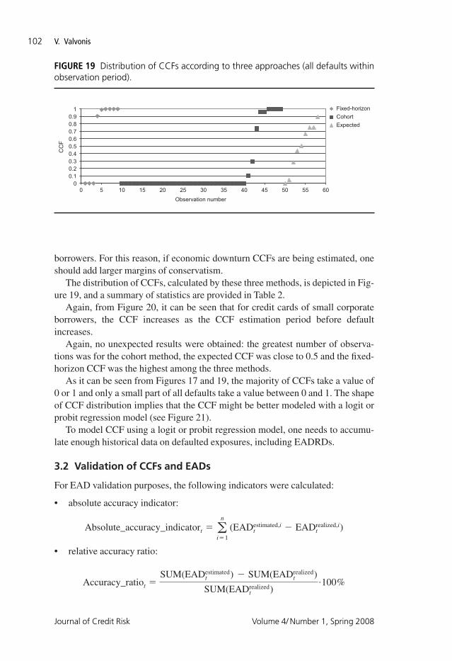
borrowers. For this reason, if economic downturn CCFs are being estimated, oneshould add larger margins of conservatism.
The distribution of CCFs, calculated by these three methods, is depicted in Fig-ure 19, and a summary of statistics are provided in Table 2.
Again, from Figure 20, it can be seen that for credit cards of small corporateborrowers, the CCF increases as the CCF estimation period before defaultincreases.
Again, no unexpected results were obtained: the greatest number of observa-tions was for the cohort method, the expected CCF was close to 0.5 and the fixed-horizon CCF was the highest among the three methods.
As it can be seen from Figures 17 and 19, the majority of CCFs take a value of0 or 1 and only a small part of all defaults take a value between 0 and 1. The shapeof CCF distribution implies that the CCF might be better modeled with a logit orprobit regression model (see Figure 21).
To model CCF using a logit or probit regression model, one needs to accumu-late enough historical data on defaulted exposures, including EADRDs.
3.2 Validation of CCFs and EADs
For EAD validation purposes, the following indicators were calculated:
Estimating EAD for retail exposures for Basel II purposes
Technical Report www.journalofcreditrisk.com
103
TABL
E 2
CC
F es
timat
ion
stat
istic
s fo
r cr
edit
card
s of
sm
all c
orpo
rate
bor
row
ers.
Tota
l Po
ol
Stan
dar
d
Tota
l N
um
ber
N
um
ber
N
um
ber
N
um
ber
N
um
ber
of
Nu
mb
er
nu
mb
erav
erag
ed
evia
tio
nn
um
ber
of
CC
Fso
f C
CFs
of
CC
Fso
f C
CFs
0 <
CC
Fso
f b
lan
k o
f d
efau
lts
CC
F*o
f C
CF*
of
CC
Fs<
0**
> 1
**�
0**
�1*
*<
1**
CC
Fs**
*
Fixe
d-ho
rizon
app
roac
h44
0.65
462
0.49
193
93
30
03
35C
ohor
t ap
proa
ch44
0.17
608
0.36
633
401
430
05
4Ex
pect
ed C
CF
appr
oach
440.
4800
60.
3183
79
00
10
835
Not
e: *
– a
fter
set
ting
CC
Fs
0 to
0 a
nd C
CFs
�1
to 1
; **
– be
fore
set
ting
CC
Fs
0 to
0 a
nd C
CFs
�1
to 1
; ***
– n
umbe
r of
mis
sing
CC
Fs (e
g, t
he C
CF
is m
issi
ng b
ecau
se it
isou
tsid
e th
e ob
serv
atio
n pe
riod
as d
efau
lt oc
curr
ed n
ear
the
boun
dary
of
the
obse
rvat
ion
perio
d or
def
ault
occu
rred
sho
rtly
aft
er t
he e
xpos
ure
was
ext
ende
d an
d th
us n
o hi
stor
ical
data
is a
vaila
ble)
.
JCR 07 05 22 VV 3/12/08 6:12 PM Page 103
3.2.1 Credit cards of private individuals
Figures 22 and 23 reveal EAD validation results for credit cards of privateindividuals.
Before going into details of validation results, it should be noted that the lastfive to six observation points should be interpreted with caution. In the last five tosix observation periods, the number of exposures decreases substantially as fewerand fewer new defaults oocur and more and more exposures move out of thesample as the 12-month observation period relevant for validation matures. Thismeans that for the last five to six observation periods the portfolio under valida-tion is unrepresentative, ie, all exposures are close to default and there are veryfew exposures that are 12, 11, 10 or so months before default. This would never
Estimating EAD for retail exposures for Basel II purposes
Technical Report www.journalofcreditrisk.com
105
0200400600800
1,0001,2001,4001,6001,8002,000
2005
.01
2005
.02
2005
.03
2005
.04
2005
.05
2005
.06
2005
.07
2005
.08
2005
.09
2005
.10
2005
.11
2005
.12
2006
.01
2006
.02
2006
.03
2006
.04
2006
.05
2006
.06
2006
.07
2006
.08
2006
.09
2006
.10
2006
.11
2006
.12
Observation time period
No.
of o
bser
vatio
ns
−60,000
−40,000
−20,000
0
20,000
40,000
60,000
80,000EUR
Number of observations(left-hand axis)
Fixed-horizon CCF = 41.2%(right-hand axis)
Cohort CCF = 12.5%(right-hand axis)
Expected CCF = 32.4%(right-hand axis)
FIGURE 22 Absolute accuracy of the methods.
0200400600800
1,0001,2001,4001,6001,8002,000
2005
.01
2005
.02
2005
.03
2005
.04
2005
.05
2005
.06
2005
.07
2005
.08
2005
.09
2005
.10
2005
.11
2005
.12
2006
.01
2006
.02
2006
.03
2006
.04
2006
.05
2006
.06
2006
.07
2006
.08
2006
.09
2006
.10
2006
.11
2006
.12
Observation time period
–15
–10
–5
0
5
10
15
20%
Number of observations(left-hand axis)
Fixed-horizon CCF = 41.2%(right-hand axis)
Cohort CCF=12.5%(right-hand axis)
Expected CCF = 32.4%(right-hand axis)
No.
of o
bser
vatio
ns
FIGURE 23 Relative accuracy of the methods.
JCR 07 05 22 VV 3/12/08 6:12 PM Page 105
happen in real life, as in reality there will always be new defaults coming into theportfolio. For the same reasons, the first observations should be excluded from thevalidation results. Summing up, from the whole observation period for validationpurposes, roughly, only the period of 2005.02–2006.07 is relevant. As more andmore historical data will be collected, the relevant validation period will increase(cut-off periods at the beginning and at the end of the whole observation periodshould stay pretty much the same).
As the CCF for the fixed-horizon method is the highest, so is the overestima-tion of true EAD on a portfolio level. Figures 22 and 23 show that on average thetrue EAD on a portfolio level is overestimated by almost €60,000 or 9%. Thisallows us to conclude that the CCF estimate is appropriate. The motivation forappropriateness of the fixed-horizon CCF � 41.2%, even for economic downturnconditions, is provided in the next paragraph.
The other two methods with lower average CCFs yield different results: theexpected CCF approach shows only slight overestimation of EAD on a portfoliolevel. This supports the conclusion in previous sections that the expected CCFmethod should be the most appropriate approach for estimating the CCF as all theinformation within a one-year time period is included in the calculation, not justone observation point as it is done with the fixed-horizon or the cohort approach.The cohort method for modeled data gives the underestimation of EAD on theportfolio level, ie, the CCF of 12.5% is too low.
From Figure 23, it can be seen that a decrease of CCF by 8.8 percentage points(the fixed-horizon approach CCF compared with the expected CCF) caused onaverage to decrease surplus of the relative accuracy ratio by 4.3 percentage points.This implies that the true CCF (the one when there is no underestimation or over-estimation of EAD on the portfolio level, ie, the relative accuracy ratio is equal to0) is approximately 18.4% (8.8% · 9%/4.3%). For example, the fixed-horizonapproach CCF is set to 41.2 or 22.8 percentage points above the true CCF. Thus, itcan be concluded that if banks would choose the fixed-horizon approach, it wouldbe very conservative for setting CCF, even for economic downturn conditions.
3.2.2 Credit cards of small corporate borrowers
Figures 24 and 25 reveal EAD validation results for credit card exposures forsmall corporate borrowers.
Validation results for credit cards of small corporate borrowers look rather sim-ilar to those for credit cards of private individuals. The only significant differencesare the following: the greater volatility of accuracy ratios and the greater elasticityof accuracy ratios to changes in CCF. For example, the comparison of cohort andexpected CCF approaches shows that a decrease of average CCF from 43.2% to17.6% or alternatively by 25.6 percentage points has lead to a decrease of relativeaccuracy ratio by 9.73 percentage points. Thus, in order to reduce 10.9% of theaverage surplus of the accuracy ratio of the expected CCF method to 0, one needsto reduce the expected CCF by 28.7 percentage points to the level of 14.5%. Inother words, having a CCF of 14.5% would lead to an accuracy ratio close to 0.
Estimating EAD for retail exposures for Basel II purposes
Technical Report www.journalofcreditrisk.com
107
0
5
10
15
20
25
3020
05.0
120
05.0
220
05.0
320
05.0
420
05.0
520
05.0
620
05.0
720
05.0
820
05.0
920
05.1
020
05.1
120
05.1
220
06.0
120
06.0
220
06.0
320
06.0
420
06.0
520
06.0
620
06.0
720
06.0
820
06.0
920
06.1
020
06.1
120
06.1
2
Observation time period
–10,000
–5,000
0
5,000
10,000
15,000
20,000
25,000EUR
Number of observations(left-hand axis)
Fixed horizon CCF = 65.5%(right-hand axis)
Cohort CCF = 17.6%(right-hand axis)
Expected CCF = 48.0%(right-hand axis)
No.
of o
bser
vatio
ns
FIGURE 24 Absolute accuracy of the methods.
0
5
10
15
20
25
30
2005
.01
2005
.02
2005
.03
2005
.04
2005
.05
2005
.06
2005
.07
2005
.08
2005
.09
2005
.10
2005
.11
2005
.12
2006
.01
2006
.02
2006
.03
2006
.04
2006
.05
2006
.06
2006
.07
2006
.08
2006
.09
2006
.10
2006
.11
2006
.12
Observation time period
–80
–60
–40
–20
0
20
40
60
80%
Number of observations(left-hand axis)
Fixed horizon CCF = 65.5%(right-hand axis)
Cohort CCF = 17.6%(right-hand axis)
Expected CCF = 48.0%(right-hand axis)
No.
of o
bser
vatio
ns
FIGURE 25 Relative accuracy of the methods.
JCR 07 05 22 VV 3/12/08 6:12 PM Page 107
Comparing elasticity or sensitivity of accuracy ratio with changes in the CCFbetween credit cards for private individuals and small corporate borrowers, it isobvious that validation results of private individuals are much more sensitive tochanges in the CCF. This implies that small corporate borrower’s credit cards’EAD validation results should be expected to fluctuate relatively less with the eco-nomic cycle, despite how much CCF changes. Moreover, empirical results revealthat EAD overestimation on a portfolio level is higher for credit cards of smallcorporate borrowers.
4 CONCLUSIONS
EAD, being one of the four IRB model parameters, is least analyzed among practi-tioners and supervisors. This paper shows that many issues on EAD modelingremain open. For example, banks are bound by supervisory requirements toestimate EAD as a function of on-balance, off-balance exposure amounts and theCCF. This precludes any other EAD modeling methods from being used in an IRBframework.
Currently, only two methods are endorsed by supervisors for calculating real-ized CCFs for defaulted exposures, namely the cohort and the fixed horizon.These two methods take into consideration only information at one point in timewhile calculating the realized CCF. However, information on how exposureevolved over one year prior to default can have a valuable input. Thus, othermethods for expressing the realized CCF for defaulted exposures must besearched. Besides, the calculation of realized CCFs for defaulted exposuresshould be aligned with a CCF modeling method for non-defaulted exposures.
CCF used for EAD estimation purposes for non-defaulted exposures should bedependent on the utilization ratio of exposure: as EAD at the time of default isfixed, so the EAD model, ceteris paribus, should give a rather stable EAD forecastfor non-defaulted exposure as the current outstanding amount changes.
Empirical CCF calculation results showed that the majority of realized CCFstake a value of either 0 or 1. This implies that while building an EAD model oneshould try to model these extreme outcomes, ie, try to model when the exposuresshall have a CCF equal to 0 or 1. For these purposes, a logit or probit regressionmodel might work well.
REFERENCES
Agarwal, S., and Ambrose, B. (2006). Credit lines and credit utilization. Journal of Money,Credit and Banking 38(1), 1–22.
Araten, M., and Jacobs, M. (2001). Loan equivalents for revolving credits and advisedlines. The RMA Journal 83(8), 34–39.
Basel Committee on Banking Supervision (2004). International convergence of capitalmeasurement and capital standards: a revised framework. Consultative Document,Bank for International Settlements, June.
Basel Committee on Banking Supervision (2005). An explanatory note on the Basel II IRBrisk weight functions. Working Paper, October.
Journal of Credit Risk Volume 4/ Number 1, Spring 2008
V. Valvonis108
JCR 07 05 22 VV 3/12/08 6:12 PM Page 108
Committee of European Banking Supervisors (2005). Guidelines on the implementation,validation and review of advanced measurement (AMA) and internal ratings based(IRB) approaches. Working Paper, July.
Department of Treasury (2003). Internal ratings-based systems for corporate credit andoperational risk advanced measurement approaches for regulatory capital. WorkingPaper, August.
EU (2006). Directive 2006/48/EC of the European Parliament and of the Council of 14June 2006 relating to the taking up and pursuit of the business of credit institutions(recast). http://eur-lex.europa.eu/LexUriServ/site/en/oj/2006/l_177/l_17720060630en00010200.pdf [14 February 2008].
Expert group on loss given default other (2005). Expert group paper on loss given defaultother. http://www.fsa.gov.uk/pubs/international/loss.pdf [14 February 2008].
Financial Supervision Authority, UK (2004a). Issues arising from policy visits on exposure atdefault in large corporate and mid market portfolios. Working Paper, September.
Financial Supervision Authority, UK (2004b). Own estimates of exposure at default. Work-ing Paper, November.
Moral, G. (2006). EAD estimates for facilities with explicit limits. The Basel II risk parame-ters: estimation, validation, and stress testing, Engelmann, B. and Rauhmeier, R. (eds.).Springer, Heidelberg, Germany, 197–242.
RMA (2004). Industry practices in estimating EAD and LGD for revolving consumer credits-cards and home equity lines of credit. Working Paper, March.
Schuermann, T. (2004). What do we know about loss given default? Working Paper No.04-01, Wharton Financial Institutions Center, February.