Estimating Fiscal Multipliers:News From a Nonlinear World�

Giovanni Caggiano Efrem CastelnuovoUniversity of Padova University of Melbourne

University of Padova

Valentina Colombo Gabriela NodariUniversity of Padova University of Verona

University of New South Wales

March 2015

Abstract

We estimate nonlinear VARs to assess to what extent �scal spending multi-pliers are countercyclical in the United States. We deal with the issue of non-fundamentalness due to �scal foresight by appealing to sums of revisions of expec-tations of �scal expenditures. This measure of anticipated �scal shocks is shownto carry valuable information about future dynamics of public spending. Resultsbased on generalized impulse responses suggest that �scal spending multipliers inrecessions are greater than one, but not statistically larger than those in expan-sions. However, nonlinearities arise when focusing on "extreme" events, i.e., deeprecessions vs. strong expansionary periods.

Keywords: Fiscal news, Fiscal foresight, Fiscal spending multiplier, SmoothTransition Vector-AutoRegressions, Extreme events.

JEL codes: C32, E32, E52.

� A shorted version of this paper has been accepted for publication in the Economic Journal. Wethank Morten O. Ravn (Editor) and two anonymous referees for their insighful comments and sug-gestions. We also thank Fabio Canova, Fabrice Collard, Marco Del Negro, Filippo Ferroni, PatrickFève, Luca Gambetti, Michal Horvath, James Morley, Giorgio Primiceri, Giovanni Ricco, Antti Ri-patti, Barbara Rossi, Timo Teräsvirta, Tugrul Vehbi, Benjamin Wong, and participants at variousseminars and conferences for their feedback. Part of this work was developed while Colombo wasvisiting the Aarhus University and Caggiano the University of Melbourne, whose hospitality is grate-fully acknowledged. Caggiano acknowledges the �nancial support received by the Visiting ResearchScholar program o¤ered by the University of Melbourne. Corresponding author: Efrem Castelnuovo,efrem.castelnuovo@unimelb.edu.au .

1 Introduction

How large is the �scal spending multiplier? Following the lead of Blanchard and Per-

otti (2002), several VAR models featuring �scal aggregates have been estimated to

answer this question (for a survey, see Ramey (2011a)). However, the quanti�cation

of �scal multipliers with standard VARs is controversial for two reasons. First, as

stressed by Parker (2011), the e¤ects of �scal policy shocks may very well be coun-

tercyclical. Fiscal multipliers may be larger in periods of slack because of a milder

crowding out of private consumption and investment due to less responsive prices (see

the textbook IS-LM-AD-AS model), a constrained reaction of nominal interest rates

due to the zero-lower bound (Eggertsson (2010), Christiano, Eichenbaum, and Rebelo

(2011), Woodford (2011), Leeper, Traum, andWalker (2011), and Fernández-Villaverde,

Gordon, Guerrón-Quintana, and Rubio-Ramírez (2012)), higher returns from public

spending due to countercyclical �nancial frictions and credit constraints (Canzoneri,

Collard, Dellas, and Diba (2015)), and lower crowding out of private employment due

to a milder increase in labor market tightness (Michaillat (2014), Roulleau-Pasdeloup

(2014)). Empirical evidence in favor of state-dependent �scal multipliers is provided by,

among others, Tagkalakis (2008), Auerbach and Gorodnichenko (2012, 2013a, 2013b),

Bachmann and Sims (2012), Batini, Callegari, and Melina (2012), Mittnik and Semmler

(2012), Baum, Poplawski-Ribeiro, and Weber (2012), Fazzari, Morley, and Panovska

(2014).1 Second, anticipation e¤ects are likely to be of great relevance in the trans-

mission of �scal policy shocks, a phenomenon often referred to as "�scal foresight"

(see, among others, Yang (2005), Fisher and Peters (2010), Mertens and Ravn (2011),

Ramey (2011b), Gambetti (2012a, 2012b), Kriwoluzky (2012), Favero and Giavazzi

(2012), Leeper, Walker, and Yang (2013), Ellahie and Ricco (2013)). Modeling a stan-

dard set of U.S. variables with a medium-scale structural model that allows for foresight

up to eight quarters, Schmitt-Grohe and Uribe (2012) �nd that about sixty percent of

the variance of government spending is due to anticipated shocks. Unfortunately, in

presence of �scal foresight, standard VARs - which rely on current and past shocks to

1Other forms of state-dependence have been identi�ed in the literature. Corsetti, Meier, and Müller(2012) investigate the sensitivity of government spending multipliers to di¤erent economic scenarios.They �nd �scal multipliers to be particularly high during times of �nancial crisis. Rossi and Zubairy(2011) and Canova and Pappa (2011) show that �scal multipliers tend to be larger when positivespending shocks are accompanied by a decline in the real interest rate. Perotti (1999) shows that �scalmultipliers may depend on the debt-to-GDP ratio in place when �scal shocks occur. For a DSGE-basedquanti�cation of �scal multipliers in presence of normal vs. abnormal debt-to-GDP ratios, see Cantore,Levine, Melina, and Pearlman (2013).

3

interpret the dynamics of the modeled variables - are typically "non-fundamental", in

that they do not embed the information related to "news shocks", i.e., future shocks

anticipated by rational agents.2 Leeper, Walker, and Yang (2013) work with a variety

of �scal models and show that the anticipation of tax policy shocks severely a¤ects VAR

exercises aiming at identifying �scal shocks. Forni and Gambetti (2010) and Ramey

(2011b) show that government spending shocks estimated with standard �scal VARs

are predictable, i.e., they are non-fundamental.

This paper estimates state-dependent �scal multipliers by explicitly addressing the

issue of �scal foresight. We tackle the issue of non-fundamentalness by jointly modeling

a measure of anticipated ("news") �scal spending shocks along with a set of standard

macro-�scal variables. Such a measure of �scal news is the sum of revisions of ex-

pectations about future government spending collected by the Survey of Professional

Forecasters. As shown by Gambetti (2012a, 2012b) and Forni and Gambetti (2014),

this measure of �scal shocks is particularly powerful to capture the e¤ects of �scal

spending shocks when the implementation lag of �scal policy is larger than one quarter,

a very plausible assumption as for U.S. �scal policy decisions.3 We include this measure

of �scal news in a nonlinear Smooth Transition Vector AutoRegressive (STVAR) model,

which we use to discriminate dynamic responses to �scal shocks in bad and good times

(i.e., recessions vs. expansions). Our multipliers are computed as the integral of the

impulse response of output (up to a chosen horizon) divided by the integral of the re-

sponse of �scal expenditure (up to the same horizon) and rescaled by the sample mean

value of the output-public spending ratio.4 To assess the e¤ects of public spending

shocks on output and estimate �scal multipliers in recessions and expansions, we com-

pute Generalized Impulse Response Functions (GIRFs), which model the endogeneity

of the transition from a state to another after a �scal shock. Importantly, as explained

by Koop, Pesaran, and Potter (1996), GIRFs allow us to scrutinize the role played by

di¤erent initial conditions. We then isolate "extreme" events, i.e., deep recessions and

2For a recent discussion on non-fundamentalness in the VAR context and a survey of the maincontributions in this area, see Beaudry and Portier (2014).

3Yang (2005) shows that the average implementation lag for major postwar U.S. income tax leg-islation is about seven months. Mertens and Ravn (2011) �nd that the median implementation lagis six quarters. Leeper, Richter, and Walker (2012) calibrate tax foresight and government spendingforesight to range between two and eight quarters (the former) and between three and four quarters(the latter).

4Our results are robust to to the employment of an alternative way of computing �scal multipliers,i.e., the ratio of the "peak" value of the impulse responses of output and public spending rescaledby the sample mean ratio of the levels of ouput over public spending. Our Appendix (available uponrequest) documents the results obtained with this alternative way of computing �scal multipliers.

4

strong expansions, with the aim of understanding if �scal multipliers are larger in very

severe economic conditions. To our knowledge, this key policy-relevant question has

not been previously studied in the empirical literature on �scal multipliers.

Our results are the following: i) anticipated �scal expenditure shocks trigger a signif-

icant reaction of output; ii) such a reaction is not statistically di¤erent across di¤erent

phases (recessions/expansions) of the U.S. business cycle; iii) the reaction becomes sta-

tistically di¤erent for extreme phases of the business cycle, i.e., deep recessions vs.

strong expansions; iv) �scal multipliers in recessions are statistically larger than one;

v) spending shocks in recessions have a noticeable stabilization e¤ect and substantially

reduce the probability that the economy will remain slack. These results are robust

to a wide battery of checks, including i) the employment of a "purged" measure of �s-

cal news, which is constructed using information available to survey respondents when

they formulate their expectations over future public spending, to account for potential

identi�cation issues; ii) the use of the �scal news constructed by Ramey (2011b), which

allows us to extend our sample back to 1947, to control for small-sample biases that may

a¤ect our data-intensive estimator; iii) the role of debt, to account for the role played

by �scal strains in computing multipliers; iv) several di¤erent VAR speci�cations.

Our paper represents a novel contribution under several respects. First, our VAR

jointly accounts for two relevant issues for the quanti�cation of �scal multipliers: �scal

foresight and state dependence. Second, we estimate the response of economic aggre-

gates to �scal shocks via GIRFs, which allow us to endogenize the possibly stabilizing

e¤ects of �scal policy. Third, the use of GIRFs allows us to address a previously unex-

plored issue, i.e., the role played by business cycle conditions for the quanti�cation of

�scal multipliers, which we investigate by distinguishing between "extreme" and "mod-

erate" business cycle phases. As a result, we are able to establish some new stylized

facts about government spending multipliers in the U.S., in particular the fact that �rm

evidence of state dependence arises only when looking at extreme phases of the business

cycle.

The closest papers to ours are Auerbach and Gorodnichenko (2012, 2013a), Owyang,

Ramey, and Zubairy (2013), and Ramey and Zubairy (2014). Auerbach and Gorod-

nichenko (2012, 2013a) employ a STVAR model and �nd evidence of countercyclical

�scal multipliers.5 There are substantial di¤erences between Auerbach and Gorod-

nichenko�s contributions and ours. First, they investigate the role of unanticipated

�scal spending shocks. Di¤erently, we focus on anticipated changes in �scal spending.

5For a similar exercise focusing on the role of business con�dence, see Bachmann and Sims (2012).

5

Second, their impulse responses are conditionally linear, i.e., expansionary �scal spend-

ing shocks are, by construction, not allowed to drive the economy out of a recession. As

pointed out by the same authors, this assumption provides an "upper bound" for their

estimates of the �scal multiplier in recessions, because it does not allow the returns from

�scal spending to be decreasing as the economy exits a recession. Our approach links

the evolution of the variables in our STVAR to the probability of being in a recession,

which is then endogenously modeled. Third, our focus is on "extreme" events, i.e., real-

izations on the tails of the distribution of our business cycle indicator (like the 2007-09

crisis). Our main result is that, while �scal multipliers may be acyclical when recessions

and expansions are considered all alike (i.e., they may be similar when considering the

average e¤ect in recessions vs. expansions), they are likely to be large in presence of par-

ticularly severe economic conditions. Owyang, Ramey, and Zubairy (2013) and Ramey

and Zubairy (2014) employ local-projection methods à la Jordà (2005) to investigate

the nonlinearity of �scal multipliers. They �nd no evidence of larger �scal multipliers

during downturns as for the United States. The comparability between our exercises

and theirs is not immediate due to a number of di¤erent modeling choices (construction

of the news shocks, length of the sample, construction of the impulse responses, among

others). We notice that our results are similar to theirs in that we also do not �nd larger

�scal multipliers in recessions on average. However, when it comes to deep recessions

vs. strong expansions, we �nd such larger multipliers to arise.

Other strands of the literature have dealt with �scal foresight and anticipated �s-

cal spending shocks in VARs. Mertens and Ravn (2010) recover the non-fundamental

responses to an anticipated �scal policy shock via economic theory-driven restrictions

to gauge information about economic agents� anticipation rate. Such a rate is then

used as an input in Blaschke matrices to �ip the roots that cause the non-invertibility

of the VMA representation of �scal spending and output. Kriwoluzky (2012) recov-

ers reduced-form innovations by estimating a VARMA model using the Kalman �lter.

Then, he identi�es anticipated �scal shocks via theoretically-supported sign restrictions.

Ramey and Shapiro (1998) follow a narrative approach to identify exogenous changes

in military spending related to wars. Ramey (2011b) constructs a measure of changes

in the expected present value of government spending. Fisher and Peters (2010) con-

struct a measure of excess returns of large U.S. military contractors which is shown to

anticipate future military spending shocks. Ben Zeev and Pappa (2014) identify U.S.

defense news shocks as the shocks that best explain future movements in defense spend-

ing over a �ve year horizon and are orthogonal to current defense spending. All these

6

contributions show that, at least qualitatively, anticipated positive �scal shocks induce a

signi�cant increase in output.6 Perotti (2007, 2011), Ramey (2011b), Gambetti (2012a,

2012b), Blanchard and Leigh (2013), Alesina, Favero, and Giavazzi (2014), Forni and

Gambetti (2014a), and Ricco (2014) work with expectations revisions in di¤erent mod-

eling frameworks. Our paper complements these contributions, in that it quanti�es the

e¤ects of anticipated �scal spending shocks with a nonlinear model focusing on extreme

events.7

The structure of the paper is the following. Section 2 deals with the issue of non-

fundamentalness in the macro-�scal context due to the presence of �scal foresight, and

explains why the sums of revisions of �scal expectations variable employed in our analy-

sis helps solving the issue. Section 3 o¤ers statistical support to the role of nonlinearities

in this context and presents the Smooth Transition VAR model employed in our analy-

sis. Our main results are shown in Section 4, which deals with the computation of

�scal multipliers in recessions and expansions, and Section 5, which focuses on extreme

events. Section 6 documents a battery of robustness checks. Concluding remarks are

provided in Section 7.

2 Non-fundamentalness and expectations revisions

The role of expectations revisions. As anticipated in our Introduction, standard�scal VARs may return severely biased impulse responses in presence of news shocks.

Consider the model

yt = �Etyt+1 + gt + !t (1)

gt = "t�h + �1"t�h�1 + : : :+ �q�h�1"t�(q�1) + �q�h"t�q = �(L)"t (2)

6Another interesting approach to account for �scal foresight rests on the use of municipal bondspreads. This bond spread is well-known to have predictive power for tax changes and can thereforebe used to control for anticipated tax changes (see, among others, Poterba (1989), Fortune (1996), andKueng (2014)). Leeper, Richter, and Walker (2012) show that spreads with maturity lengths of 1 and5 years are very informative about future tax events. Our paper deals with anticipated �scal spendingshocks. We leave the analysis of anticipated tax shocks to future research.

7Admittedly, the theoretical papers modeling nonlinearities cited in this Introduction mainly con-sider models in which government spending is implemented without lags. As for the zero lower bound,however, Christiano, Eichenbaum, and Rebelo (2011) conduct an exercise in which they model imple-mentation lags in their framework featuring the zero lower bound. They �nd that a key determinantof the size of the multiplier is indeed the state of the world in which new government spending comeson line. Our conjecture is that such asymmetric e¤ects may be present also when anticipated �scalshocks hit economic systems characterized by state-dependent �nancial constraints and labor marketdownward rigidities.

7

where j�j < 1; �i > 0 8i; h � 0; q � h, and �0 = 0. The forward-looking process yt- say, output measured as log-deviations from its trend - is a¤ected by the exogenous

stationary process gt - say, a �scal process - plus a random shock !t, which is assumed

to capture non-�scal spending shocks a¤ecting output and which is assumed to be i:i:d:

with zero mean and unit variance. The process (2) features q � h + 1 moving averageterms. If h = 0 and q > 0, the process (2) features an unanticipated, "t; as well

as anticipated shocks "t�q for q > 0. For h > 0, the process (2) would feature only

anticipated shocks, where h is the number of periods of foresights. The process gt is a

news-rich process if j�ij > 1 for at least one i > 0 (Beaudry and Portier (2014)). In

all cases, f"t�jgqj=h is said to be fundamental for gt if the roots of the polynomial �(L)lie outside the unit circle (Hansen and Sargent (1991)). Importantly, if the gt process

is non-fundamental, its structural shock is not recoverable by employing current and

past realizations of gt only. Consequently, its impulse response to an anticipated shock

as well as the dynamic responses of other variables �in this example, yt �will not be

correctly recovered by estimating a VAR in yt and gt.

We assume that agents have rational expectations and observe news shocks without

noise.8 It can be shown that, if the period of foresight h > 1 is known, the problem of

non-fundamentalness in model (1)-(2) can be solved by alternatively including: i) the

h-step-ahead expectation, Etgt+h; if h = q; ii) the h-step-ahead expectation revision,

Etgt+h�Et�1gt+h; if h < q. However, if h > 1 is unknown, expectation revisions are notof help. To solve this issue, Gambetti (2012a) proposes to use a news variable de�ned

as

�g1J =XJ

j=1(Etgt+j � Et�1gt+j) =

� �1 + �1 + :::+ �J�h

�"t if J < q�

1 + �1 + :::+ �q�h�"t if J > q

; (3)

which correctly identi�es the news shock if J > h.9 Our Appendix provides further

discussions and derivations as regards this news variable.8Forni, Gambetti, Lippi, and Sala (2013) investigate the case in which economic agents deal with

noisy news. Agents are assumed to receive signals regarding the future realization of TFP shocks.Since such signals are noisy, agents react not only to genuinely informative news, but also to noiseshocks that are unrelated to economic fundamentals. They �nd that such noise shocks explain about athird of the variance of output, consumption, and investment. We leave the quanti�cation of the roleof noise shocks in the �scal context to future research.

9If J < h; the news variable would have no predictive content about �scal shocks, and it wouldbe equal to zero. In our sample, however, this never happens. This is consistent with the evidencein Leeper, Richter, and Walker (2012), who report an average implementation lag of about threequarters. In our example above, h should be interpreted as the minimum temporal gap between theannouncement of the implementation of future �scal spending and the realization of the spending itself(which may take more than one quarter), rather than the mean value. Hence, also the e¤ects of theannouncement of future spending whose full implementation would take more than J quarters wouldbe captured by our news, as long as the minimum lag h is less than J .

8

The News13 variable. We will then consider a �scal VAR augmented with a

measure of news constructed by summing up revisions of expectations as follows:

�g13 =X3

j=1(Etgt+j � Et�1gt+j) (4)

where Etgt+j is the forecast of the growth rate of real government spending from period

t+ j � 1 to period t+ j based on the information available at time t. Hence, Etgt+j �Et�1gt+j represents the "news" that becomes available to private agents between time

t � 1 and t about the growth rate of government spending j periods ahead. We usedata coming from the Survey of Professional Forecasters (SPF), which collects forecasts

conditional on time t � 1 of variables up to time t + 3. This is the reason why ourbaseline analysis will be conducted by considering the variable �g13.

10

Information content of expectations revisions. To assess the statistical rel-evance of our news variable for the dynamics of public expenditure, we regress public

spending on a constant and three lags of the dependent variable, public receipts, real

GDP, and one lag of the measure of news �g13 (a detailed description of the data is

provided in Section 3). This regression augments the public spending equation of a

trivariate VAR system modeling the "usual suspects" (public spending, tax receipts,

output) with our news variable lagged one period.11 Public spending shocks are often

identi�ed with a Cholesky decomposition of the covariance matrix of the VAR residuals.

Hence, the (orthogonalized) residuals of the public spending equation are interpreted

as public spending shocks. As shown in Table 1 - which collects the p-values for our �g13variable in the equation described above - news shocks are found to carry signi�cant in-

formation about the future evolution of public spending. This implies that the trivariate

�scal VAR without news is non-fundamental. Digging deeper, we �nd that all the three

components (forecast revisions) included in �g13 have some predictive power. Overall,

this empirical exercise highlights the signi�cant contribution of news revisions regarding

future realizations of public expenditure. Di¤erently, revisions of expectations based on

nowcasting, i.e., Etgt � Et�1gt, turn out to be insigni�cant at the 90% con�dence level

(see Table 1, last column). In line with Ricco (2014), this result suggests that revisions

based on "nowcasts" (revision of expectations at time t of contemporaneous public ex-

10SPF data are a¤ected by frequent changes in the base years. Forecast errors on the growth ratesare not a¤ected by these changes. Hence, they are preferable to forecast errors computed with SPFlevels. About this point, see also Perotti (2011).11The regression includes variables in (log-)levels and the news �g13 variable in cumulated sums to

preserve the same order of integration. This is consistent with the modeling choices of our baselineVAR analysis (speci�ed in the next Section).

9

penditures) are possibly of help in identifying truly unanticipated �scal shocks, rather

than anticipated, news shocks.12

Overall, our results i) show that, from a statistical standpoint, residuals typically

employed in a standard trivariate �scal VAR cannot be interpreted as �scal shocks;

ii) suggest that the components of the variable �g13, which we interpret as a measure

of anticipated �scal shocks, can augment the information content of our VAR system.

These results are consistent with the outcome of the Granger-causality tests conducted

by Gambetti (2012b), who shows that �g13 Granger-causes �scal spending at di¤erent

horizons.13

Extreme realizations of the news spending variable: An interpretation.Figure 1 plots our news variable (an updated version of Gambetti�s 2012b). The stan-

dardized variable �g13 conveys useful information about �scal policy shocks in the United

States. To see this, we isolate the seven realizations which exceed two in absolute value,

and provide an interpretation based on the recent U.S. �scal history. The 1983Q1

positive realization is associated to Ronald Reagan�s "Evil Empire" and "Star Wars"

speeches, with which the U.S. President announced a forthcoming increase in military

spending. The 1986Q1 negative spike re�ects the speech given in January 1986 by

Mikhail Gorbachev, who proposed decommissioning all nuclear weapons by 2000 in the

early stage of the "Perestrojka" period. The 1987Q1 positive forecast revisions might

be due to the mid-term Senate elections won by the Democrats in November 1986 plus

the questioned constitutionality of the Gramm-Rudman-Hollings Balanced-Budget Act.

The 1987Q4 forecast revisions are due to announcements about spending cuts for the

Pentagon. The fall of the Berlin Wall in November 1989 is behind the negative spike in

1989Q4. The war in Afghanistan rationalizes the positive peak in 2001Q4. Finally, the

upward spike in 2009Q1 can be associated to Obama�s stimulus package.

Comparison with Ramey�s (2011b) news variable. Figure 1 also plots themilitary spending news variable constructed by Ramey (2011b), and extended up to

12These results are conditional on news variables constructed as revisions of the mean predictedvalues of the levels of future government spending as collected by the Survey of Professional Forecast-ers. Similar results were obtained by employing median values of such forecasts, as well as variablesexpressed in growth rates.13In a recent paper, Perotti (2011) questions the use of the SPF forecast errors employed by Ramey

(2011) to isolate �scal spending anticipated shocks. In particular, he shows that the one-step-aheadpredictive power of the forecast revisions as for federal spending is quite modest, since such revisionsare shown to be noisy. Our results are fully consistent with Perotti�s (2011) analysis, in that we alsoreject the relevance of very short-term SPF forecast revisions on future �scal spending. This evidencesuggests the need of searching for anticipation e¤ects beyond one-quarter relative to the moment inwhich predictions are formulated, and supports the employment of a variable like �g13.

10

2010Q4 by Owyang, Ramey, and Zubairy (2013).14 It appears that the �g13 variable

anticipates changes in Ramey�s, or at least it is not anticipated by the latter. To cor-

roborate this statement, we run Granger-causality tests based on an estimated bivariate

VAR with one lag involving the military spending news proposed by Ramey (2011b) (as

well as its updated version by Owyang, Ramey, and Zubairy, 2013) and the �g13 variable.

Table 2 collects the outcome (p-values associated to testing the null hypothesis that the

column variable does not Granger-cause the alternative news measure) of this exercise

for our benchmark sample and a shorter sample to account for the fact that, for the �rst

�ve years in the benchmark sample, Ramey�s (2011b) variable is equal to zero. While

the contribution of our news shock variable �nds large statistical support, Granger-

causality running from Ramey�s shock to ours is clearly rejected by the data. The same

evidence emerges when employing the news variable by Owyang, Ramey, and Zubairy

(2013), which includes observations related to the 2007-2009 recession. Again, these

results are in line with those reported in Gambetti (2012b), who also �nds Ramey�s

news shock to be predicted by forecast revisions over one quarter.

3 Econometric approach: A STVAR macro-�scalmodel

Modeling choices. We assess the state-dependence of �scal spending multipliers tonews shocks by estimating a Smooth-Transition VAR model (for an extensive presen-

tation, see Teräsvirta, Tjøstheim, and Granger (2010)). Our STVAR framework reads

as follows:

X t = F (zt�1)�R(L)X t + (1� F (zt�1))�E(L)X t + "t; (5)

"t � N(0;t); (6)

t = F (zt�1)R + (1� F (zt�1))E; (7)

F (zt) = exp(� zt)=(1 + exp(� zt)); > 0; zt � N(0; 1): (8)

where X t is a set of endogenous variables which we aim to model, F (zt�1) is a

transition function which captures the probability of being in a recession, regulates

the smoothness of the transition between states, zt is a transition indicator, �R and�E

14Ramey (2011b) employs Business Week and other newspaper sources to construct an estimate ofchanges in the expected present value of goverment spending (nominal spending divided by nominalGDP one period before).

11

are the VAR coe¢ cients capturing the dynamics of the system during recessions and

expansions (respectively), "t is the vector of reduced-form residuals having zero-mean

and whose time-varying, state-contingent variance-covariance matrix is t, and Rand E stand for the covariance structure of the residuals in recessions and expansions,

respectively. The modeling assumption is that the variables can be described with a

combination of two linear VARs, one suited to describe the economy during recessions

and the other during expansions. The transition from a state to another is regulated

by the standardized transition variable zt. The smoothness parameter a¤ects the

probability of being in a recession F (zt), i.e., the larger the value of , the faster the

transition from a state to another. Notably, the model (5)-(8) allows for nonlinearities

to arise from both the contemporaneous and the dynamic relationships of the economic

system.

Our baseline analysis refers to the vector X t = [Gt; Tt; Yt; �g13;t]

0, where G is the log

of real government (federal, state, and local) purchases (consumption and investment),

T is the log of real government receipts of direct and indirect taxes net of transfers to

business and individuals, and Y is the log of real GDP.15 The construction of G and T

closely follows Auerbach and Gorodnichenko (2013a).16 The variable �g13 is the public

expenditure news variable (4). The variables are expressed in levels because of possible

cointegration relationships. Consistently, the variable �g13 is considered in cumulated

sums to preserve the same order of integration as the other variables included in the

vector. Our sample of U.S. data spans the period 1981Q3-2013Q1, 1981Q3 being the

�rst available quarter to construct the news variable.17

The choice of the transition variable zt and the calibration of the smoothing para-

meter are justi�ed as follows. As in Auerbach and Gorodnichenko (2012), Bachmann

and Sims (2012), Caggiano, Castelnuovo, and Groshenny (2014), and Berger and Vavra

(2014), we employ a standardized moving average of the real GDP quarter-on-quarter

15Our �scal aggregates are constructed using the Bureau of Economic Analysis�NIPA Table 3.1.Current tax receipts are constructed as the di¤erence between current receipts and government socialbene�ts. Fiscal expenditure is the sum of consumption expenditure and gross government investmentfrom which we subtract the consumption of �xed capital. Data on real GDP and the implicit GDPde�ator (which we use to de�ate all nominal series) are provided by the Federal Reserve Bank of St.Louis.16Auerbach and Gorodnichenko (2013a) check and verify the robustness of the results in Auerbach

and Gorodnichenko (2012) to the employment of a di¤erent de�nition of the net tax series that avoidsthe double-counting of mandatory Social Security contributions.17Our interpretation of the news variable here is that of an instrument to gauge the real e¤ects of

anticipated changes in �scal spending. We recall that di¤erent identi�cation approaches may very welllead to the construction of di¤erent, but in principle equally valid, instruments. For an elaboration ofthis point, see Favero and Giavazzi (2012).

12

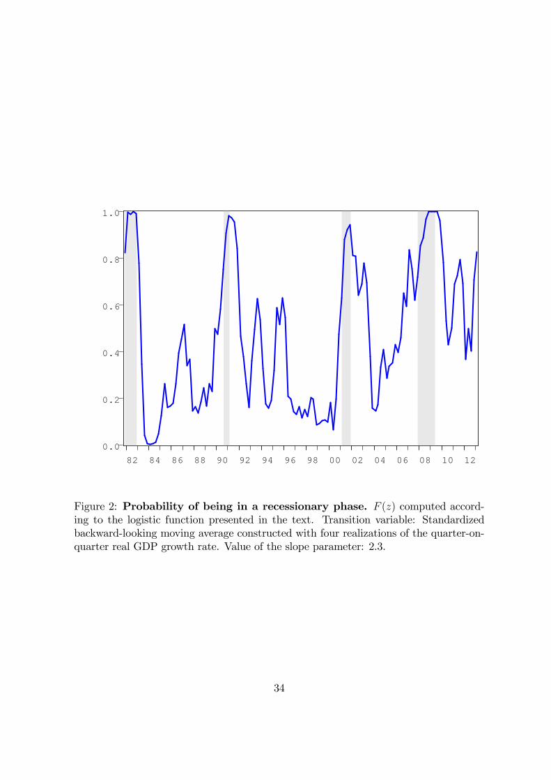
percentage growth rate.18 We calibrate the smoothness parameter to match the ob-

served frequencies of the U.S. recessions as identi�ed by the NBER business cycle dates,

i.e. 15% in our sample. Then, we de�ne as "recession" a period in which F (zt) > 0:85,and calibrate to obtain Pr(F (zt) > 0:85) � 15%. This metric implies a calibration

= 2:3. The choice is consistent with the threshold value z = �0:75% discriminat-

ing recessions and expansions, i.e., realizations of the standardized transition variable z

lower (higher) than the threshold will be associated to recessions (expansions).19 Figure

2 plots the transition function F (zt). Clearly, high realizations of F (zt) tend to be as-

sociated with NBER recessions. Importantly, our results are robust to the employment

of alternative calibrations of the slope parameter that imply a number of recessions in

our sample ranging from 10% to 20%, where the lower bound is determined by the min-

imum amount of observations each regime should contain according to Hansen (1999)

(checks not shown here for the sake of brevity, but available upon request).

Identi�cation of the anticipated �scal shock. Following Fisher and Peters

(2010), we order the news variable �g13 last in our vector and orthogonalize the reduced-

form residuals of the VAR via a Cholesky-decomposition of the variance-covariance

matrix. We analyze the implications of this versus alternative strategies to identify

�scal news shocks in Section 5.

Statistical evidence in favor of nonlinearity. For our vector of endogenousvariables Xt, we test and clearly reject the null hypothesis of linearity in favor of the

(Logistic) Smooth Transition Vector AutoRegression via the multivariate test proposed

by Teräsvirta and Yang (2013) in presence of a single transition variable. Details on

this test and its implementation are presented in our Appendix.

Model estimation. Given the high nonlinearity of the model, we estimate it

via the Monte-Carlo Markov-Chain algorithm developed by Chernozhukov and Hong

(2003). The (linear/nonlinear) VARs include three lags. This choice is based on the

Akaike criterion applied to a linear model estimated on the full-sample 1981Q3-2013Q1.

18The transition variable zt is standardized to render our calibration of comparable to thoseemployed in the literature. We employ a backward-looking moving average involving four realizationsof the real GDP growth rate.19The corresponding threshold value for the non-standardized moving average real GDP growth rate

is equal to 0.34%. The sample mean of the non-standardized real GDP growth rate in moving averageterms is equal to 0.71, while its standard deviation is 0.50. Then, its corresponding threshold valueis obtained by "inverting" the formula we employed to obtain the standardized transition indicator z,i.e., znonstd = �0:75� 0:50 + 0:71 = 0:34:

13

4 Generalized impulse responses and �scal multi-pliers

This Section reports the estimated impulse responses to an anticipated �scal spending

shock. Following Koop, Pesaran, and Potter (1996), we compute generalized impulse

responses to take into account the interaction between the evolution of the variables in

the vector Xt and the transition variable, the latter being directly in�uenced by the

evolution of output. In other words, we model the feedback from the evolution of output

in the vectorXt to the transition indicator zt and, consequently, the probability F (zt�1).

Hence, in computing our GIRFs, the probability F (z) is endogenized.20 Koop, Pesaran,

and Potter (1996) and Ehrmann, Ellison, and Valla (2003) show that initial conditions

a¤ect the computation of the GIRFs. In our benchmark exercise, we randomize over

all possible histories within each state, so to control for the role of initial conditions.21

We compute the GIRFs by normalizing the news shocks to one.22

GIRFs. Figure 3 reports the impact of a government spending news shock computedwith our linear and nonlinear VARs. The responses obtained with our linear model point

to a delayed short-run increase in government expenditure and output, and a decrease

in government receipts. Public spending reaches its peak value after about three years.

Di¤erently, output increases for the �rst three quarters after the shock, then gradually

goes back to zero, and crosses the zero line about 10 quarters after the shock.

20Recall that our transition indicator zt � 14 (�Yt +�Yt�1 +�Yt�2 +�Yt�3), i.e., the relationship

between zt and �Yt�i; i = 0; 1; 2; 3 features no stochastic elements. Hence, stochastic singularityprevents us from estimating our model jointly with the evolution of zt. Following Koop, Pesaran, andPotter (1996), our GIRFs are based on simulations that take into account the link between Xt and ztafter the estimation of our econometric framework.21Following Koop, Pesaran, and Potter (1996), our GIRFs are computed as follows. First, we draw

an initial condition, i.e., starting values for the lags of our VARs as well as the transition indicator z,which - given the logistic function (8) - gives us the value for F (z). Then, we simulate two scenarios,one with all the shocks identi�ed with the Cholesky decomposition of the VCV matrix (7), and anotherone with the same shocks plus a � > 0 corresponding to the �rst realization of the news shock. Thedi¤erence between these two scenarios (each of which accounts for the evolution of F (z) by keepingtrack of the evolution of output and, therefore, z) gives us the GIRFs to a �scal news shock �. Pereach given initial condition z, we compute 500 di¤erent stochastic realizations of our GIRFs, thenstore the median realization. We repeat these steps until 500 initial conditions (drawn by allowing forrepetitions) associated to recessions (expansions) are considered. Then, we construct the distributionof our GIRFs by considering these 500 median realizations. Our Appendix provides details on thealgorithm we employed to compute the GIRFs.22The standard deviation of the news variable employed in the sample is 0.19 according to our linear

model, 0.21 conditional on our framework under recessions, and 0.18 under expansions. While beingtheoretically size-dependent, we veri�ed that the sensitivity of our impulse responses to reasonablechanges in the size of the shock is negligible.

14

Next, we look at the evidence coming from the nonlinear VAR. Interestingly, the

estimated response of output is persistently stronger under recessions. Output increases

in expansions in the short-run, but the increase is much milder compared to recessions,

and vanishes after about four quarters. Another di¤erence between the two states is

the reaction of government spending itself, which is always positive but stronger in

recessions. Tax receipts react asymmetrically in the short run, then their patterns

become more similar.

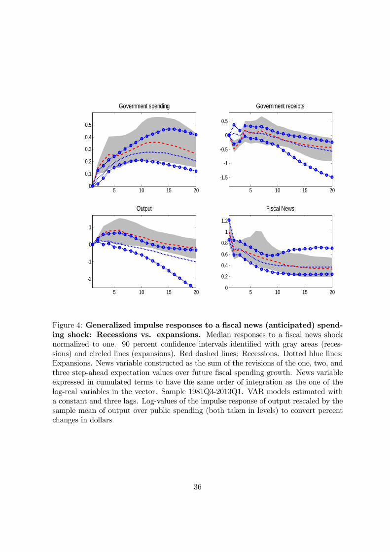
Are the reactions of output in recessions and expansions di¤erent from a statistical

standpoint? Figure 4 plots the GIRFs and the associated 90% con�dence intervals es-

timated for both states. Focusing on output, we see that the con�dence bands overlap

substantially. This result suggests that the reaction of output to a �scal shock is not

necessarily stronger if the economy is slack. This �nding is in line with some recent re-

sults put forth by Valerie Ramey and coauthors (see Ramey (2011b), Owyang, Ramey,

and Zubairy (2013) and Ramey and Zubairy (2014)), which are obtained with a di¤er-

ent identi�cation strategy (�scal spending news shocks constructed following Ramey�s

(2011b) approach) and methodology (local projections à la Jordà (2005)). At a �rst

glance, the evidence seems to be at odds with the impulse response analysis proposed by

Auerbach and Gorodnichenko (2012, 2013a), who �nd a statistically signi�cant di¤er-

ence between the response of output conditional on di¤erent states. However, a subtle

di¤erence in the construction of the dynamic responses must be considered. Auerbach

and Gorodnichenko (2012, 2013a) assume the economy hit by the �scal shock to start

and remain in a recession/expansion for twenty quarters. Di¤erently, here we allow the

economic system to switch from a state to another according to the endogenous evolu-

tion of the transition indicator. Moreover, the GIRFs plotted in Figure 4 are constructed

by integrating over all histories belonging to a given state (recessions, expansions). We

elaborate on the role played by initial conditions in Section 5.

Quantifying the multipliers. We now turn to the key issue of computing themultipliers and the associated 90% con�dence intervals. We compute the "sum" (cu-

mulative) multiplier as the integral of the response of output divided by the integral of

the response of �scal expenditure, i.e.,PH

h=1 Yh=PH

h=1Gh, where H is a chosen horizon.

Percent changes are then converted into dollars by rescaling such a ratio by the sample

mean ratio of the levels of output over public spending.23 This measure is designed to

23Ramey and Zubairy (2014) warn against this practice by noticing that, in a long U.S. data samplespanning the 1889-2011 period, the output-over-public spending ratio varies from 2 to 24 with a meanof 8. Hence, the choice of a constant value for such ratio may importantly bias the estimation of themultipliers. In our sample, the mean value of such a ratio is 6, and it varies from 5.39 to 6.76. Hence,

15

account for the persistence of �scal shocks (Woodford (2011)).

Our results are reported in Table 3, where multipliers have been computed consid-

ering horizons from one to �ve years. The evidence clearly speaks in favor of larger

(short-run) �scal spending multipliers in recessions, with values between 3.05 after 8

quarters and 1.00 after 20 quarters. The point-estimates of our multipliers in expan-

sions are substantially lower (from 0.33 to -2.27 after 8 and 20 quarters, respectively).

The multipliers under recession are statistically larger than one in the short run (i.e.,

for the �rst four quarters).

Are multipliers statistically bigger in recessions? We answer this question by con-

structing a test based on the di¤erence between the multiplier estimated under reces-

sions and expansions. Such a test is constructed to account for the correlation between

the estimated state-dependent multipliers.24 Figure 5 plots the distribution of the dif-

ference of our multipliers for a range of horizons of our impulse responses along with

90% con�dence bands. Evidence in favor of state-dependent multipliers would be gained

if zero were not included in the con�dence bands. In all cases, although marginally, the

di¤erence turns out to be not di¤erent from a statistical standpoint.25

The stabilizing e¤ects of anticipated �scal shocks. Our STVAR allows alsoto estimate the impact of government spending shocks on the probability of being in a

recession for each given horizon of interest after the shock. Figure 6 plots the estimated

transition function implied by our model, [F (z); along with the 90% con�dence bands.

The Figure gives interesting information about the estimated impact of a positive gov-

ernment spending shock on the likelihood of remaining in the same phase of the business

cycle. Looking at the behavior of the [F (z) under recession, we notice that the �scalshock leads to a clear drop in the probability of remaining in recession. Given the large

the commonly adopted ex-post conversion from the estimated elasticities to dollar increases does notappear to be an issue for our exercise. The average value of the output-public spending ratio in oursample in 5.81 in NBER recessions, and 6.02 in NBER expansions. Our results are robust to theemployment of state-dependent output-public spending ratios.24In short, we compute di¤erences of our multipliers in recessions vs. expansions conditional on

the same set of draws of the stochastic elements of our model as well as the same realizations of thecoe¢ cients of the vector. The empirical density of the di¤erence between our multipliers is based on500 realizations of such di¤erences for each horizon of interest.25Importantly, our results are not driven by the systematic component of our STVAR per se. In

other words, in absence of �scal interventions, our model economy does not deliver large negativeaccumulated multipliers at longer forecast horizons when starting in expansions. This was veri�ed bysimulating a deterministic version of the STVAR, in which only initial conditions are responsible forthe di¤erent evolution of the variables in recessions and expansions. Our simulations con�rm that ourcumulated multipliers are indeed driven by the interaction between �scal shocks and the systematiccomponent of our STVARs.

16

uncertainty surrounding the response of output to a �scal shock, di¤erent paths of [F (z)are admittedly possible. However, the median indication clearly suggests a quick fall

of such a probability under the threshold value F = 0:85 just after �ve quarters, which

is exactly the average duration of a NBER recession in the sample. In terms of the

econometric methodology employed to estimate the state-dependent e¤ect of govern-

ment spending shocks on output, this evidence shows the importance of allowing for the

possibility of switching from one phase of the business cycle to another. Unsurprisingly,

given its expansionary e¤ect, the probability of falling into a recession after the news

shock when starting from an expansions is basically zero, though such a probability is

quite imprecisely estimated.

5 Fiscal multipliers in presence of "extreme" events

Extreme events analysis. So far, our analysis has focused on the possible state-dependence of output reactions to �scal news shocks and �scal multipliers, �nding weak

evidence in favor of countercyclical spending multipliers. The next question we address

is whether evidence of nonlinearities might arise when recessions and expansions are "ex-

treme" events. We then re-compute the GIRFs by randomizing over di¤erent subsets of

histories associated to recessions and expansions. We label "deep" recessions/"strong"

expansions the histories associated to realizations of the transition variable which are be-

low/above two standard deviations. Given that our transition variable is standardized,

this amounts to saying that all historical realizations of z above two are associated to a

strong expansion, while all realizations below minus two are associated to a deep reces-

sion. This criterion leads us to isolate four realizations in deep recessions corresponding

to the recent great recession (2008Q4-2009Q3) and three realizations which belong to

the "strong" expansions category (1983Q4-1984Q2). In a complementary fashion, mild

recessions/weak expansions are associated to histories consistent with realizations of

the transition variable below/above the threshold value z = �0:75 but within the range[�2; 2]. We then re-compute the GIRFs by randomizing over histories within each ofthese four sub-categories.

Figure 7 shows the GIRFs obtained by distinguishing between "deep" and "mild"

recessions and "strong" and "weak" expansions. The estimated GIRFs show that the

response of output is roughly proportional to the strength of the recession (expansion).

Although in the short-run the response of output in the case of a "mild" recession is very

similar to the response of output in a "deep" recession, the response of output is much

17

more persistent at longer horizons when conditioning on the latter case. This, however,

cannot be immediately turned into evidence about multipliers, since the persistence in

output response might be driven by the persistence of government spending.

Table 4 reports the �scal multipliers estimated in the four di¤erent cases under

scrutiny. Interestingly, multipliers are still larger in recessions relative to expansions,

regardless of the strength of the recession (expansion). When the economy is in a deep

recession, we �nd the 4-year horizon multiplier to be 1.6. A similar �gure can be gauged

for mild recessions, where government spending is found to be expansionary after up

to four years. In strong expansions, short-run (one-year) multipliers are slightly above

one, but they take negative values at longer horizons. Interestingly, while the di¤erence

between mild recessions and weak expansions might seem minimal, the impact of �scal

policy in these two states is much more dramatic. Such a di¤erence may be interpreted

in light of the di¤erent response of �scal revenues in the two states (at least in the short-

run). In good times, government receipts are found to increase after the shock, while in

bad times they are found to decrease. In other words, our VAR suggests that recessions

are associated to de�cit-�nanced increases in public spending, while expansions are

associated to increases in �scal spending which are readily �nanced via an increase in

revenues. Hence, recessions are associated with a higher net present value of the �scal

de�cit relative to expansions. This can justify the large and positive real e¤ects of �scal

news on the output multiplier if, during recessions, the Ricardian equivalence does not

hold because of, say, binding liquidity constraints during recessions, of rule-of-thumb

consumers. It can also o¤er a rationale for the negative multipliers in strong expansions,

which is a state associated with a clearly positive response of revenues to �scal spending

shocks.26

Turning to multipliers in expansions, while our point estimates suggest values above

one in the short-run, 90% con�dence bands imply that we cannot reject values lower

than unity. A possible interpretation of large short-run multipliers in expansions relates

to the zero lower bound, which has been in place even after the end of the 2007-09

recession, hence in a period classi�ed as ("weak") expansion in our sample. As shown

by Leeper, Traum, and Walker (2011), multipliers may be larger than one when an

active �scal policy is accompanied by a passive monetary policy.27

26See Barro and Redlick (2011) for a discussion of de�cit-�nanced versus balanced-budget �scalmultipliers.27In our sample, the number of quarters associated to expansions by the NBER in which the zero

lower bound is in place is 15, i.e., some 14% of all the quarters in expansions according to the NBER,which is a non-negligible share. For an analysis pointing to lower �scal spending multipliers in a

18

When we turn to statistical di¤erence, a comparison between the multipliers in the

case of "deep" recessions and those conditional on "strong" expansions suggests that the

con�dence bands do not overlap, and point to a strong evidence in terms of nonlinear

responses of the economy to an expansionary �scal shock. Our results are con�rmed also

by looking at the distribution of the di¤erence between the estimated state-dependent

multipliers. As shown in Figure 8, the countercyclicality of �scal multipliers conditional

on extreme realizations of the business cycle is supported regardless of the horizon.

In our context, it might be more appropriate to test for the null hypothesis of equal

multipliers versus the one-sided alternative of multipliers larger in recessions relative to

expansions. Table 5 collects the fraction of multipliers that are larger in recessions for

both "Normal" (recessions/expansions) and "Extreme" (deep recessions/strong expan-

sions) phases of the business cycle. As before, these numbers are estimated by referring

to di¤erent initial conditions, all else being equal. Hence, any entry greater than or

equal to 90 might be interpreted as evidence in favor of larger multipliers in recessions

at a 90% con�dence level in the context of a one-sided test. The �gures corresponding

to the exercises conducted so far refer to the "Baseline" scenario. Under the "Normal"

(i.e. all recessions vs. all expansions) case, evidence in favor of countercyclical multipli-

ers is not present for all horizons. Di¤erently, the analysis of extreme events robustly

points towards larger multipliers during recessions. We postpone the analysis of the

robustness of this result to a number of perturbations of the baseline framework to the

next Section.

How does the economic system evolve after a �scal shock hitting during an extreme

phase of the business cycle? Figure 9 plots the estimated value of the [F (z) conditionalon the four scenarios. For deep recessions, a sizeable decrease of the probability of

remaining in such a state occurs as a consequence of the government spending shock:

after about �ve quarters, the value of [F (z) decreases from 1 (the economy is in a reces-sion with probability one) to about 0.5 (the economy is unlikely to be in a recession).

This drop is quicker and more substantial than the one estimated in presence of mild

recessions, and it is also more precisely estimated. Importantly, this suggests that gov-

ernment spending can be e¤ective in lifting the U.S. economy from a deep recession

to an expansionary path. The probability of moving away from a strong expansion is

low, and more precisely estimated than the one of drifting away from a weak expansion.

However, none of the two suggests a high likelihood of falling into a recession.

liquidity trap caused by a self-ful�lling state of low con�dence in a model with nominal rigidies and aTaylor-type interest rate rule, see Mertens and Ravn (2014).

19

Estimated multipliers: Comparison with the literature. Our evidence pointsto larger multipliers in recessions (around 1.6 for the 4-year horizon), and smaller ones,

but still somewhat high in the short-run (slightly larger than 1 after one year), in expan-

sions. Are these multipliers in line with what suggested by the literature? A close look

at some recent contributions suggests a positive answer. Auerbach and Gorodnichenko

(2012, 2013a) deal with unexpected �scal shocks in a nonlinear VAR framework and

�nd multipliers in recessions of about 2.5. Bachmann and Sims (2012) control for the

e¤ects of business con�dence and �nd the sum and peak multipliers in recessions to be

2.7 and 3.3, respectively. Corsetti, Meier, and Müller (2012) work with a �exible panel

of OECD countries that allow them to study the e¤ects of �scal spending shocks under

di¤erent scenarios. Conditional on periods of �nancial strains, they �nd �scal spending

multipliers to be 2.3 on impact, 2.9 at the peak, and larger than 2 in the medium run.28

Christiano, Eichenbaum, and Rebelo (2011) work with a medium-scale DSGE model

and �nd a multiplier of 2.3 conditional on the zero-lower bound being in place for one

year. Evidence of large multipliers can be found also in linear frameworks which deal

with the issue of �scal foresight. Using Bayesian prior predictive analysis for a battery

of closed- and open-economy DSGE models featuring di¤erent frictions and policy con-

ducts, Leeper, Traum, and Walker (2011) rationalize �scal spending multipliers of two

or larger. Ben Zeev and Pappa (2014) �nd a peak multiplier larger than 4. Fisher and

Peters (2010), using their measure of excess returns of large U.S. military contractors,

�nd a multiplier of 1.5. The same �gure is found by Ricco (2014), who employes a

measure of news which accounts for the changes in the composition of the pool of fore-

casters compiling the SPF questionnaires. Depending on the set of restrictions imposed

in their sign restriction-VAR analysis, Canova and Pappa (2011) �nd the U.S. �scal

multipliers to range between 2 and 4.

Our �ndings qualify those by Auerbach and Gorodnichenko (2012, 2013a), who

suggest that recessions are associated with larger �scal spending multipliers. As already

pointed out, their general conclusion might be driven by the implicit assumption that

all recessions are treated like "extreme events" when conducting their impulse response

analysis. Our analysis suggests that this may very well be the case. This �nding has

important implications from a policy perspective too, given that a �scal stimulus may

be needed exactly in correspondence to deep recessions.

28As reported in the minutes of the Economic Policy Panel Discussion, Giancarlo Corsetti pointedout that �nancial crises, in their study, are not meant to represent recessions. However, he also addedthat the multipliers are even larger when one uses macro crisis episodes alone in their panel approach.See Economic Policy, 2012, 27(72), p. 562.

20

Overall, our analysis based on "disaggregated" recessions and expansions shows that

nonlinearities are likely to arise when we look within each of the two states typically

investigated in a business cycle context, i.e., recessions and expansions. In particular,

we �nd support in favor of a larger �scal multiplier when deep recessions are considered.

6 Further investigations

Our baseline analysis suggests that evidence in favor of countercyclical �scal multipliers

is borderline when we condition upon recessions vs. expansions, while it becomes much

clearer and solid when conditioning upon extreme events. This Section discusses the

solidity of our results to the employment of i) alternative identi�cation strategies; ii) a

longer sample; iii) debt; iv) several di¤erent VAR speci�cations.

6.1 Identi�cation

Exogeneity of the change in government spending expectations. Our baselineanalysis rests on revisions of government spending expectations. Such revisions may in

principle be due to shocks other than merely �scal ones. Suppose that gt = �zt + �t,

where zt is a vector of m indicators of the business cycle (say, output, unemployment,

in�ation, interest rates), � is the vector of loadings relating zt to gt, and �t = "t +

�1"t�1+�2"t�2+ :::+�n"t�n is a moving average process modeling the unexpected �scal

shock "t as well as the expected ones "t�j; j = 1; :::; n. Then, �g13 =X3

j=1(Etgt+j �

Et�1gt+j) = �X3

j=1(Etzt+j � Et�1zt+j) + e�g13, where e�g13 = X3

j=1�j"t�j. In words,

systematic revisions of �scal spending forecasts might be due not only to anticipated

�scal shocks, but also to revisions of other variables� forecasts possibly due to other

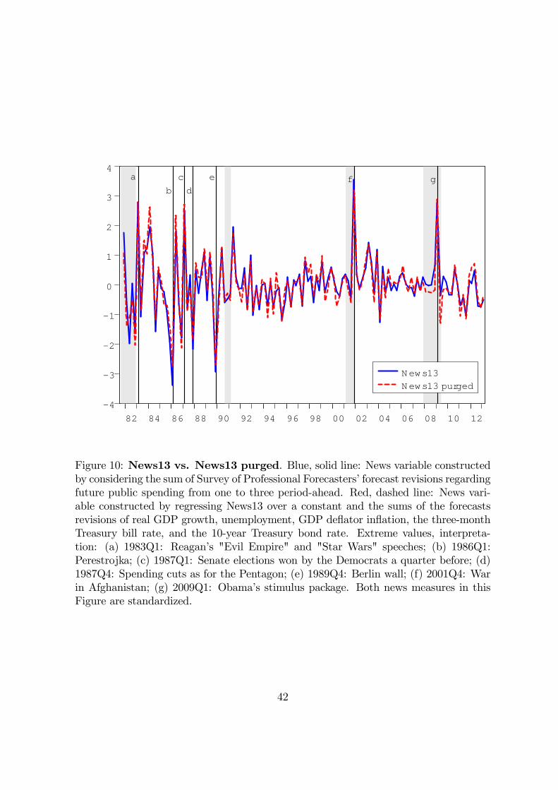
shocks (technology, �nancial). We deal with this issue by regressing our measure of �scal

news �g13 on a number of macroeconomic indicators available to professional forecasters

when they are asked to form expectations about G: (the sums of forecasts revisions of)

real GDP growth, unemployment, GDP de�ator in�ation, the 3-month Treasury bill

rate, and the 10-year Treasury bond rate.29 Figure 10 displays the raw and purged

29Forecasts of the debt-to-GDP ratio are not included in the SPF survey. We run further regressionsby adding lagged realizations of debt-to-GDP ratio to the regression described in the text. Suchmeasures turn out to be insigni�cant. The choice of not including the contemporaneous realizationsof the debt-to-GDP ratio on the right-hand side of the regression is due to the timing of the Surveyof Professional Forecasters (SPF). The questionnaire of such survey is sent to the pool of respondentsafter the advance report of the national income and product accounts by the Bureau of EconomicAnalysis (BEA) is released to the public. Hence, the questionnaire contains the �rst estimate of GDP

21

versions of the news variable, denoted by �g13 and e�g13 respectively. Two considerationsare in order. First, the correlation between these two variables is quite high (0.95).

Second, the most extreme realizations, documented in Figure 1 and reproposed here,

are clearly captured by both variables. Hence, most of the information content of the

(unpurged version of the) �g13 variable is likely to come from its genuinely exogenous

component. To corroborate this statement, we replace the �g13 variable with its purged

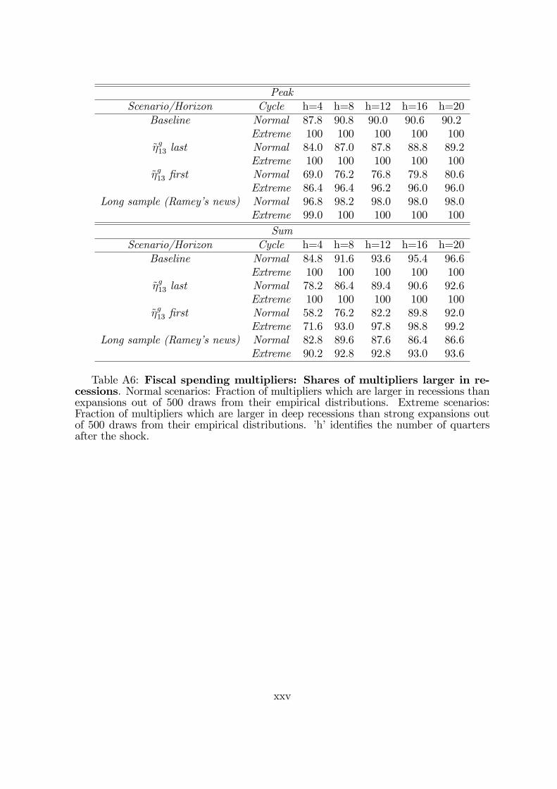
version e�g13 in our VAR, and re-run our estimations and simulations. Table 6 ("e�g13 last")collects the results of this exercise for our extreme events analysis.30 These results, as

well as those in Table 5 on the di¤erence of the multipliers in extreme business cycle

phases, con�rm our baseline �ndings

Contemporaneous e¤ects of �scal spending shocks. Another issue a¤ectingour baseline analysis regards the timing of the impact of the news shocks. The baseline

vector features a recursive identi�cation scheme in which the news variable is ordered

last. This choice aims at purging the movements of the �g13 �scal variable by accounting

for its systematic response to government spending, tax revenues, and output. However,

such a choice has an obvious limitation, i.e., output is not allowed to move immediately

after the realization of the news shock. We then perform a robustness check by focusing

on the four-variate VAR Xe�gt = [e�g13;t; Gt; Tt; Yt]0, which enables �scal news shocks to

a¤ect output on impact.31 We run this exercise with our purged measure of anticipated

�scal shocks to control for the systematic movements of �scal news due to news hitting

other macroeconomic indicators, as explained above. Table 6 ("e�g13 �rst") documentsslightly di¤erent, but statistically equivalent, multipliers relative to the baseline. Most

importantly, as also documented by Table 5, we �nd again larger multipliers in deep

recessions than in strong expansions.

and its components for the previous quarter. Thus, in formulating and submitting their projections,the information sets of the SPF panelists include the data reported in the advance report and related toquarter t�1 but not data regarding quarter t. For information on the variables included in the surveyand the information set possessed by respondents, see http://www.philadelphiafed.org/research-and-data/real-time-center/survey .30Multipliers computed by considering a four-year time span. Similar results are obtained when

considering a two-year time span.31An alternative, not pursued here, would be to work with sign restrictions. For an analysis of sign

restrictions in �scal VARs and their implications for the implied �scal elasticities, see Caldara andKamps (2012).

22

6.2 Longer sample

The nonlinear estimator we employ is data intensive. Because of limited data avail-

ability for the SPF forecast revisions, our baseline analysis rests on a relatively short

sample, i.e., 1981Q3-2013Q1. Hence, small-sample issues may lead to distortions of our

estimated coe¢ cients, which could then lead us to obtain biased multipliers. We then

conduct a robustness check by employing a much longer sample, i.e., 1947Q1-2013Q1.

To do so, we use an updated version of Ramey�s (2011b) widely known �scal news vari-

able (available at Valerie Ramey�s website), and put it �rst in a VAR including �scal

spending, �scal revenues, and output. Following Ramey (2011b), we estimate a VAR

with four lags and a quadratic trend. Table 6 ("Long sample, Ramey�s news") collects

the outcome of our estimations. Reassuringly, this exercise produces multipliers very

much in line with our baseline ones, and it o¤ers support to the importance of looking

at extreme events to �nd nonlinearities in the �scal multipliers even in long samples.

6.3 The role of debt

Our baseline VAR does not feature debt. However, controlling for debt �uctuations

in our regressions is important to better understand the drivers of our countercyclical

multipliers. The reason is simple. Recent panel-data studies have shown that countries

with "high" levels of debt have smaller multipliers than countries with lower levels of

debt (see, e.g., Corsetti, Meier, and Müller (2012), Ilzetzki, Mendoza, and Végh (2013)).

Hence, it could in principle be possible that the nonlinearities we have found are driven

by di¤erent levels of debt rather than di¤erent phases of the business cycle. It is then of

interest to check if the relevant initial conditions could be related to di¤erent degrees of

�scal distress. To this aim, we modify our baseline vector along two dimensions. First,

we include the debt/GDP ratio in our VAR. Following a common modeling choice in

the literature (see, among others, Leeper, Traum, and Walker (2011), Leeper, Richter,

and Walker (2012), Corsetti, Meier, and Müller (2012), and Leeper, Walker, and Yang

(2013)), we assume the debt/GDP ratio to a¤ect the �scal instruments with a lag,

and put it last in the vector. Second, we employ our debt/GDP ratio as the variable

which dictates the switch from a regime to another. This second modi�cation is exactly

aimed at capturing the idea of di¤erent "debt-contingent" regimes. To discriminate

between "high" vs. "low" realizations of debt, we focus on the cyclical component of

the debt/GDP ratio, which is extracted from the raw series (in log) by applying a stan-

dard Hodrick-Prescott �lter with smoothing weight equal to 1,600. Realizations of the

23

debt/GDP ratio one standard deviation above (below) the HP-trend are interpreted

as phases of "high" ("low") debt. Positive (negative) realizations within one standard

deviation are classi�ed as "moderately high" ("moderately low"). A possible interpreta-

tion of this series is that of a "debt/GDP gap" computed by considering a time-varying

debt/GDP target, which may be consistent with the clear upward-trending behavior

displayed by this ratio in our sample.

Table 6 ("Debt/GDP ratio") collects the multipliers produced by this exercise. We

distinguish between extreme phases of "high" and "low" �scal distress, as well as in-

termediate ones, i.e. "moderately high" and "moderately low", which we indicate with

"Mod:+ debt" and "Mod:� debt", respectively. Our results point to fairly similar �scal

multipliers when computed conditional on "high" vs. "low" debt levels. Hence, coun-

tercyclical �scal multipliers do not seem to be guided by the "�scal cycle".32 Our results

echo those by Favero and Giavazzi (2012), who also �nd no major empirical di¤erences

in a �scal model for the U.S. when adding debt. It is important to stress, however, that

this conclusion is not inconsistent with cross-country studies which point to relevant

nonlinearities of �scal policy e¤ects due to di¤erent levels of debt, in particular for

developing countries.

6.4 Further robustness checks

Our results are robust to a variety of further perturbations of our baseline model, which

include: i) a "FAST-VAR" (Factor Augmented Smooth Transition-VAR) version of our

VAR model, which we estimate to further control for non-fundamentalness as suggested

by Forni and Gambetti (2014b); ii) the estimation of a �ve-variate VAR featuring the

sum of forecast revisions regarding future real GDP as �rst variable in the vector, again

to control for revisions of real GDP forecasts; iii) the employment of revisions over total

spending forecasts (as opposed to Federal spending only); iv) a measure of news which

accounts for the changes in the composition of the pool of forecasters compiling the SPF

questionnaires as in Ricco (2014).33 The solidity of our baseline results is con�rmed also

by this battery of robustness checks, which is available upon request.

32An analysis conducted by adding the debt-to-GDP ratio to our otherwise baseline framework whilekeeping the moving average of real GDP as our transition indicator returned multipliers very similarto our baseline ones.33We thank Giovanni Ricco for providing us with his measure of �scal news.

24

7 Conclusions

This paper quanti�es the �scal spending multiplier in the U.S. and tests the theoret-

ical prediction of a larger reaction of output to �scal shocks in economic downturns.

Following Gambetti (2012a,b) and Forni and Gambetti (2014), we tackle the issue

of non-fundamentalness due to �scal foresight by identifying anticipated government

spending shocks via sums of forecasts revisions collected by the Survey of Professional

Forecasters. We show that such a measure of �scal spending news carries relevant

information to predict the future evolution of �scal expenditures and Granger-causes

other measures of �scal news recently proposed in the literature. Then, we augment a

macro-�scal nonlinear VAR with this measure of �scal news and estimate the size of

�scal spending multipliers across di¤erent phases of the business cycle.

Our empirical investigation points to �scal multipliers larger than one in recessionary

periods. However, conditional on a standard "recessions vs. expansions" classi�cation

of the phases of the U.S. business cycle, our results do not support the idea of a coun-

tercylical �scal multiplier. Di¤erently, when we condition the estimates of the �scal

multipliers on the strength of the business cycle (namely, when we distinguish between

deep and mild recessions, and weak and strong expansions), we �nd that �scal multi-

pliers are statistically larger in deep recessions relative to strong expansionary periods.

The results of our paper highlight the relevance of the di¤erent initial economic

conditions within each of the two states typically considered for classifying the U.S.

business cycle. Fiscal multipliers may very well be larger when a �scal shock occurs

in presence of a deep recession like that of 2007-09 than when it occurs in presence

of milder economic downturns. Our results imply that a correct measurement of the

�scal multipliers can be performed just if �exible-enough econometric models are put

at work.

ReferencesAlesina, A., C. Favero, and F. Giavazzi (2014): �The Output E¤ect of FiscalConsolidations,�Journal of International Economics, forthcoming.

Auerbach, A., and Y. Gorodnichenko (2012): �Measuring the Output Responsesto Fiscal Policy,�American Economic Journal: Economic Policy, 4(2), 1�27.

(2013a): �Corrigendum: Measuring the Output Responses to Fiscal Policy,�American Economic Journal: Economic Policy, 5(3), 320�322.

Auerbach, A., and Y. Gorodnichenko (2013b): �Output Spillovers from FiscalPolicy,�American Economic Review Papers and Proceedings, 103, 141�146.

25

Bachmann, R., and E. Sims (2012): �Con�dence and the transmission of governmentspending shocks,�Journal of Monetary Economics, 59, 235�249.

Barro, R. J., and C. J. Redlick (2011): �Macroeconomic E¤ects from GovernmentPurchases and Taxes,�Quarterly Journal of Economics, 126(1), 51�102.

Batini, N., G. Callegari, and G. Melina (2012): �Successful Austerity in theUnited States, Europe and Japan,�IMF Working Paper No. 12-190.

Baum, A., M. Poplawski-Ribeiro, and A. Weber (2012): �Fiscal Multipliers andthe State of the Economy,�International Monetary Fund Working Paper No. 12/286.

Beaudry, P., and F. Portier (2014): �News Driven Business Cycles: Insights andChallenges,�Journal of Economic Literature, forthcoming.

Ben Zeev, N., and E. Pappa (2014): �Chronicle of a War Foretold: The Macroeco-nomic E¤ects of Anticipated Defense Spending Shocks,�European University Insti-tute, mimeo.

Berger, D., and J. Vavra (2014): �Measuring How Fiscal Shocks A¤ect DurableSpending in Recessions and Expansions,� American Economic Review Papers andProceedings, 104(5), 112�115.

Blanchard, O., and D. Leigh (2013): �Growth Forecast Errors and Fiscal Multi-pliers,�American Economic Review Papers and Proceedings, 103(3), 117�120.

Blanchard, O., and R. Perotti (2002): �An Empirical Characterization of the Dy-namic E¤ects of Changes in Government Spending and Taxes on Output,�QuarterlyJournal of Economics, 117(4), 1329�1368.

Caggiano, G., E. Castelnuovo, and N. Groshenny (2014): �Uncertainty Shocksand Unemployment Dynamics: An Analysis of Post-WWII U.S. Recessions,�Journalof Monetary Economics, 67, 78�92.

Caldara, D., and C. Kamps (2012): �The Analytics of SVARs: A Uni�ed Frameworkto Measure Fiscal Multipliers,�Finance and Economics Discussion Series, Board ofGovernors of the Federal Reserve System.

Canova, F., and E. Pappa (2011): �Fiscal policy, pricing frictions and monetaryaccommodation,�Economic Policy, 26(68), 555�598.

Cantore, C., P. Levine, G. Melina, and J. Pearlman (2013): �Optimal Fiscaland Monetary Rules in Normal and Abnormal Times,�University of Surrey Discus-sion Paper No. 05/13.

Canzoneri, M., F. Collard, H. Dellas, and B. Diba (2015): �Fiscal Multipliersin Recessions,�CEPR Discussion Paper No. 10353.

Chernozhukov, V., and H. Hong (2003): �An MCMC Approach to Classical Esti-mation,�Journal of Econometrics, 115(2), 293�346.

Christiano, L. J., M. Eichenbaum, and S. Rebelo (2011): �When is the Govern-ment Spending Multiplier Large?,�Journal of Political Economy, 119(1), 78�121.

26

Corsetti, G., A. Meier, and G. J. Müller (2012): �What Determines GovernmentSpending Multipliers?,�Economic Policy, 27(72), 521�565.

Eggertsson, G. B. (2010): �What Fiscal Policy Is E¤ective at Zero Interest Rates?,�in Daron Acemoglu and Michael Woodford (Eds): NBER Macroeconomics Annual2010, Volume 25, 59�112.

Ehrmann, M., M. Ellison, and N. Valla (2003): �Regime-dependent impulseresponse functions in a Markov-switching vector autoregression model,�EconomicsLetters, 78(3), 295�299.

Ellahie, A., and G. Ricco (2013): �Government Spending Reloaded: InformationalInsu¢ ciency and Heterogeneity in Fiscal VARs,�London Business School, mimeo.

Favero, C. A., and F. Giavazzi (2012): �Measuring Tax Multipliers: The NarrativeMethod in Fiscal VARs,�American Economic Journal: Economic Policy, 4(2), 69�94.

Fazzari, S. M., J. Morley, and I. Panovska (2014): �State-Dependent E¤ects ofFiscal Policy,�Studies in Nonlinear Dynamics & Econometrics, forthcoming.

Fernández-Villaverde, J., G. Gordon, P. Guerrón-Quintana, and J. F.Rubio-Ramírez (2012): �Nonlinear Adventures at the Zero Lower Bound,�NBERWorking Paper No. 18058.

Fisher, J. D. M., and R. Peters (2010): �Using Stock Returns to Identify Govern-ment Spending Shocks,�Economic Journal, 120, 414�436.

Forni, M., and L. Gambetti (2010): �Fiscal Foresight and the E¤ects of GovernmentSpending,�CEPR Discussion Paper No. 7840.

(2014a): �Government Spending Shocks in Open Economy VARs,� CEPRDiscussion Paper No. 10115.

(2014b): �Su¢ cient information in structural VARs,� Journal of MonetaryEconomics, 66, 124�136.

Forni, M., L. Gambetti, M. Lippi, and L. Sala (2013): �Noisy News in BusinessCycles,�CEPR Discussion Paper No. 9601.

Fortune, P. (1996): �Do Municipal Bonds Yields Forecast Tax Policy?,�New EnglandEconomic Review, September/October, 29�48.

Gambetti, L. (2012a): �Fiscal Foresight, Forecast Revisions and the E¤ects of Govern-ment Spending in the Open Economy,�Universitat Autonoma de Barcelona, mimeo.

(2012b): �Government Spending News and Shocks,�Universitat Autonomade Barcelona, mimeo.

Hansen, B. E. (1999): �Testing for Linearity,�Journal of Economic Surveys, 13(5),551�576.

Hansen, L. P., and T. J. Sargent (1991): �Two Di¢ culties in Interpreting VectorAutoregressions,� in L. P. Hansen and T. J. Sargent (Eds.): Rational ExpectationsEconometrics, Westview Press, Boulder, CO, 77�119.

27

Ilzetzki, E., E. G. Mendoza, and C. A. Végh (2013): �How big (small?) are �scalmultipliers?,�Journal of Monetary Economics, 60, 239½U254.

Jordà, O. (2005): �Estimation and Inference of Impulse Responses by Local Projec-tions,�American Economic Review, 95(1), 161�182.

Koop, G., M. Pesaran, and S. Potter (1996): �Impulse response analysis innonlinear multivariate models,�Journal of Econometrics, 74, 119�147.

Kriwoluzky, A. (2012): �Pre-announcement and Timing: The E¤ects of a Govern-ment Expenditure Shock,�European Economic Review, 56, 373�388.

Kueng, L. (2014): �Tax News: Identifying Tax Expectations from Municipal Bondswith an Application to Household Consumption,�NBER Working Paper No. 20437.

Leeper, E. M., A. W. Richter, and T. B. Walker (2012): �Quantitative E¤ectsof Fiscal Foresight,�American Economic Journal: Economic Policy, 4(2), 115�144.

Leeper, E. M., N. Traum, and T. B. Walker (2011): �Clearing Up the FiscalMultiplier Morass,�NBER Working Paper No. 17444.

Leeper, E. M., T. B. Walker, and S.-C. S. Yang (2013): �Fiscal Foresight andInformation Flows,�Econometrica, 81(3), 1115�1145.

Mertens, K., and M. O. Ravn (2010): �Measuring the Impact of Fiscal Policy inthe Face of Anticipation: A Structural VAR Approach,� Economic Journal, 120,393�413.

(2011): �Understanding the Aggregate E¤ects of Anticipated and Unantici-pated Tax Policy Shocks,�Review of Economic Dynamics, 14(1), 27�54.

(2014): �Fiscal Policy in an Expectations Driven Liquidity Trap,�Review ofEconomic Studies, forthcoming.

Michaillat, P. (2014): �A Theory of Countercyclical Government Multiplier,�Amer-ican Economic Journal: Macroeconomics, 6(1), 190�217.

Mittnik, S., and W. Semmler (2012): �Regime Dependence of the Fiscal Multi-plier,�Journal of Economic Behavior and Organization, 83, 502�522.

Owyang, M., V. A. Ramey, and S. Zubairy (2013): �Are Government SpendingMultipliers Greater During Periods of Slack? Evidence from 20th Century HistoricalData,�American Economic Review Papers and Proceedings, 103(3), 129�134.

Parker, J. A. (2011): �On Measuring the E¤ects of Fiscal Policy in Recessions,�Journal of Economic Literature, 49(3), 703�718.

Perotti, R. (1999): �Fiscal policy in good times and bad,� Quarterly Journal ofEconomics, 114(4), 1399�1436.

(2007): �In Search of the Transmission Mechanism of Fiscal Policy,� in D.Acemogly, K. Rogo¤, and M. Woodford (Eds.): NBER Macroeconomics Annual, 22,169�226.

28

(2011): �Expectations and Fiscal Policy: An Empirical Investigation,�BocconiUniversity, mimeo.

Poterba, J. M. (1989): �Tax Reform and the Market for Tax-Exempt Debt,�RegionalScience and Urban Economics, 19(3), 537�562.

Ramey, V. A. (2011a): �Can Government Purchases Stimulate the Economy?,�Jour-nal of Economic Literature, 49(3), 673�685.

(2011b): �Identifying Government Spending Shocks: It�s All in the Timing,�Quarterly Journal of Economics, 126(1), 1�50.

Ramey, V. A., and M. D. Shapiro (1998): �Costly capital reallocation and thee¤ects of government spending,� Carnegie-Rochester Conference Series on PublicPolicy, 48, 145�194.

Ramey, V. A., and S. Zubairy (2014): �Government Spending Multipliers in GoodTimes and in Bad: Evidence from U.S. Historical Data,�University of California atSan Diego and Texas A&M University, mimeo.

Ricco, G. (2014): �A New Identi�cation of Fiscal Shocks Based on the InformationFlow,�London Business School, mimeo.

Rossi, B., and S. Zubairy (2011): �What Is the Importance of Monetary and FiscalShocks in Explaining U.S. Macroeconomic Fluctuations?,�Journal of Money, Creditand Banking, 43(6), 1247�1270.

Roulleau-Pasdeloup, J. (2014): �The Government Spending Multiplier in a Reces-sion with a Binding Zero Lower Bound,�University of Lausanne, mimeo.

Schmitt-Grohe, S., and M. Uribe (2012): �What�s News in Business Cycles,�Econometrica, 80(6), 2733�2764.

Tagkalakis, A. (2008): �The E¤ects of Fiscal Policy on Consumption in Recessionsand Expansions,�Journal of Public Economics, 92(5-6), 1486�1508.

Teräsvirta, T., D. Tjøstheim, and C. W. Granger (2010): �Modeling NonlinearEconomic Time Series,�Oxford University Press.

Teräsvirta, T., and Y. Yang (2013): �Speci�cation, Estimation and Evaluationof Vector Smooth Transition Autoregressive Models with Applications,�CREATES,Aaruhs University, mimeo.

Woodford, M. (2011): �Simple Analytics of the Government Expenditure Multi-plier,�American Economic Journal: Macroeconomics, 3(1), 1�35.

Yang, S.-C. S. (2005): �Quantifying Tax E¤ects Under Policy Foresight,�Journal ofMonetary Economics, 52(8), 1557�1568.

29

News (1; 3) (1; 1) (2; 2) (3; 3) (0; 0)p� value 0:00 0:00 0:00 0:00 0:11

Table 1: Anticipated �scal spending shocks: Statistical relevance. P-valuesrelated to the exclusion Wald-test of one period-lagged News variables entering (one ata time) a regression involving government spending (dependent variable), a constant,three lags of government spending, three lags of �scal receipts, and three lags of realGDP. Figures in bold are associated to a predictive power of news found to be sig-ni�cant at a 10 percent con�dence level. News are expressed in cumulated terms tohave an order of integration comparable to that of the other variables. Estimationconducted by considering Newey-West standard errors robust to heteroskedasticity andserial correlation.

Sample Ramey �g13 ORZ �g131981:III-2008:IV 0:44 0:061986:IV-2008:IV 0:28 0:021981:III-2010:IV 0:71 0:061986:IV-2010:IV 0:59 0:02

Table 2: News à la Ramey vs. forecast revisions: Granger-causality tests.�Ramey�stands for the news variable employed by Ramey (2011), �ORZ�stands for itsupdated version employed by Owyang, Ramey, and Zubairy (2013). P-values relatedto the exclusion Wald-test of one period-lagged covariate of interest. Figures in boldare associated to a predictive power of news found to be signi�cant at a 10 percentcon�dence level. Results based on a bivariate VAR with one lag. Null hypothesis:Column variable does not Granger cause the alternative news measure.

Horizon=State Expansion Recession4 1:73

[0:52;3:50]3:15

[1:71;4:27]

8 0:33[�1:05;2:77]

3:05[0:68;4:70]

12 �0:57[�2:24;1:54]

2:13[0:13;3:82]

16 �1:41[�3:96;0:74]

1:54[�0:42;2:95]

20 �2:27[�6:23;�0:01]

1:00[�0:94;2:47]

Table 3: Fiscal spending multipliers. Figures conditional on our baseline VARanalysis. Log-values of the impulse response of output rescaled by the sample mean ofoutput over public spending (both taken in levels) to convert percent changes in dollars.

30

Hor:=State Strong exp: Deep rec: Weak exp: Mild rec:4 1:03

[�0:51;2:03]3:42

[2:05;4:35]1:69

[0:64;3:40]3:09

[1:71;4:14]

8 �0:26[�2:01;0:84]

3:42[1:22;5:14]

0:30[�0:87;2:83]

2:94[0:56;4:46]

12 �1:32[�3:68;�0:03]

2:21[0:61;3:54]

�0:62[�2:15;1:48]

2:06[0:03;3:78]

16 �2:26[�5:63;�0:78]

1:60[0:18;2:63]

�1:40[�3:91;0:65]

1:38[�0:48;3:02]

20 �3:28[�7:00;�1:56]

1:09[�0:31;2:07]

�2:37[�6:08;0:01]

0:83[�0:97;2:54]

Table 4: Fiscal spending multipliers: Extreme events. Figures conditional onour VAR analysis with GIRFs conditional on four di¤erent sets of initial conditions.Log-values of the impulse response of output rescaled by the sample mean of outputover public spending (both taken in levels) to convert percent changes in dollars.

Scenario/Horizon Cycle h=4 h=8 h=12 h=16 h=20Baseline Normal 84.8 91.6 93.6 95.4 96.6

Extreme 100 100 100 100 100~�g13 last Normal 78.2 86.4 89.4 90.6 92.6

Extreme 100 100 100 100 100~�g13 �rst Normal 58.2 76.2 82.2 89.8 92.0

Extreme 71.6 93.0 97.8 98.8 99.2Long sample (Ramey�s news) Normal 82.8 89.6 87.6 86.4 86.6

Extreme 90.2 92.8 92.8 93.0 93.6

Table 5: Fiscal spending multipliers: Shares of multipliers larger in recessions.Normal scenarios: Fraction of multipliers which are larger in recessions than expansionsout of 500 draws from their empirical distributions. Extreme scenarios: Fraction ofmultipliers which are larger in deep recessions than strong expansions out of 500 drawsfrom their empirical distributions. �h�identi�es the number of quarters after the shock.

31

Scenario=State Strong exp: Deep rec: Weak exp: Mild rec:Baseline �2:26

[�5:63;�0:78]1:60

[0:18;2:63]�1:40

[�3:91;0:65]1:38

[�0:48;3:02]e�g13 last �1:57[�2:92;�0:91]

2:28[1:23;3:10]

�0:44[�1:97;2:29]

2:16[0:22;3:00]e�g13 first �0:70

[�2:50;0:43]2:36

[0:99;4:29]0:66

[�1:04;2:90]2:50

[0:59;4:39]

Long sample (Ramey�s news) 0:15[�0:24;0:53]

1:74[0:08;3:92]

0:07[�1:23;0:96]

1:52[0:60;4:62]

High debt Mod:+ debt Mod:� debt Low debtDebt=GDP ratio 0:68

[0:15;1:37]0:74

[�1:02;1:15]1:33

[0:95;1:66]1:33

[0:81;1:97]

Table 6: Fiscal spending multipliers: Extreme events. Di¤erent Scenarios.Four-year integral multipliers. Figures conditional on our VAR analysis with GIRFsconditional on four di¤erent sets of initial conditions. Log-values of the impulse responseof output rescaled by the sample mean of output over public spending (both taken inlevels) to convert percent changes in dollars.

32

­8

­6

­4

­2

0

2

4

6

82 84 86 88 90 92 94 96 98 00 02 04 06 08 10 12

News13O wyang,Ram ey,Zubairy

a

b

c

d

e f g

Figure 1: News13 (this paper) vs. Owyang, Ramey, and Zubairy�s (2013)news variable. Blue, solid line: News variable constructed by considering the sum ofSurvey of Professional Forecasters�forecast revisions regarding future public spendingfrom one-to-three quarter-ahead. Extreme values, interpretation: (a) 1983Q1: Reagan�s"Evil Empire" and "Star Wars" speeches; (b) 1986Q1: Perestrojka; (c) 1987Q1: Senateelections won by the Democrats a quarter before; (d) 1987Q4: Spending cuts as forthe Pentagon; (e) 1989Q4: Berlin wall; (f) 2001Q4: War in Afghanistan; (g) 2009Q1:Obama�s stimulus package. Red, dashed line: News variable constructed by Owyang,Ramey, and Zubairy (2013), who extended Ramey�s (2011) news variable up to 2010Q4.Ramey�s (2011) variable is constructed by considering the present discounted value ofexpected changes in defense spending (nominal spending divided by nominal GDP oneperiod before). Both news measures in this Figure are standardized.

33

0.0

0.2

0.4

0.6

0.8

1.0

82 84 86 88 90 92 94 96 98 00 02 04 06 08 10 12

Figure 2: Probability of being in a recessionary phase. F (z) computed accord-ing to the logistic function presented in the text. Transition variable: Standardizedbackward-looking moving average constructed with four realizations of the quarter-on-quarter real GDP growth rate. Value of the slope parameter: 2.3.

34

5 10 15 200

0.1

0.2

0.3

0.4Government Spending

5 10 15 20­0.8

­0.6

­0.4

­0.2

0

0.2Government Receipts

5 10 15 20­1

­0.5

0

0.5

1Output

5 10 15 200.2

0.4

0.6

0.8

1Fiscal News

LinearExpansionRecession

Figure 3: Generalized impulse responses to a �scal news (anticipated) spend-ing shock: Linear model, recessions, expansions. Median responses to a �scalnews shock normalized to one. News variable constructed as the sum of the revisionsof the one, two, and three step-ahead expectation values over future �scal spendinggrowth. News variable expressed in cumulated terms to have the same order of inte-gration as the one of the log-real variables in the vector. Log-values of the impulseresponse of output rescaled by the sample mean of output over public spending (bothtaken in levels) to convert percent changes in dollars.

35

5 10 15 200

0.1

0.2

0.3

0.4

0.5

Government spending

5 10 15 20

­1.5

­1

­0.5

0

0.5

Government receipts

5 10 15 20

­2

­1

0

1

Output

5 10 15 200

0.2

0.4

0.6

0.8

1

1.2

Fiscal News

Figure 4: Generalized impulse responses to a �scal news (anticipated) spend-ing shock: Recessions vs. expansions. Median responses to a �scal news shocknormalized to one. 90 percent con�dence intervals identi�ed with gray areas (reces-sions) and circled lines (expansions). Red dashed lines: Recessions. Dotted blue lines:Expansions. News variable constructed as the sum of the revisions of the one, two, andthree step-ahead expectation values over future �scal spending growth. News variableexpressed in cumulated terms to have the same order of integration as the one of thelog-real variables in the vector. Sample 1981Q3-2013Q1. VAR models estimated witha constant and three lags. Log-values of the impulse response of output rescaled by thesample mean of output over public spending (both taken in levels) to convert percentchanges in dollars.

36

­2 0 2 4 6 80

40

80

120h = 4

­5 0 5 100

40

80

120h = 8

­5 0 5 100

40

80

120h = 12

­5 0 5 100

40

80

120h = 16

­5 0 5 10 150

40

80

120h = 20

Figure 5: Di¤erence in multipliers between recessions and expansions: Allhistories. Empirical densities of the di¤erences computed as multipliers in recessionsminus multipliers in expansions. Densities constructed by considering all recessions andexpansions (initial conditions) present in the sample. Multipliers conditional on thesame set of draws of the stochastic elements of our STVAR model as well as the samerealizations of the coe¢ cients of the vector. Densities based on 500 realizations of suchdi¤erences per each horizon of interest. �h�identi�es the number of quarters after theshock.

37

5 10 15 200

0.1

0.2

0.3

0.4

0.5

0.6

0.7

0.8

0.9

1F(z) Expansion

5 10 15 200

0.1

0.2

0.3

0.4

0.5

0.6

0.7

0.8

0.9

1F(z) Recession

Figure 6: Evolution of the probability of being in a recessionary phase F(z)consistent with our GIRFs. Solid lines: Median reactions. Blue dotted/red dashedlines: 90 percent con�dence intervals. Black dashed horizontal line: Threshold value toswitch from a regime to another. Probability computed according to the logistic functionpresented in the text and the evolution of output conditional on a �scal news shock.Transition variable: Standardized backward-looking moving average constructed withfour realizations of the quarter-on-quarter real GDP growth rate. Value of the slopeparameter: 2.3.

38

5 10 15 200

0.1

0.2

0.3

0.4

0.5Government spending

5 10 15 20­1

­0.5

0

0.5Government receipts

5 10 15 20­2

­1.5

­1

­0.5

0

0.5

1Output

5 10 15 200

0.2

0.4

0.6

0.8

1Fiscal News

LinearStrong expansionDeep recessionMild recessionWeak expansion

Figure 7: Generalized impulse responses to a �scal news (anticipated) spend-ing shock: Linear model, deep vs. mild recessions, strong vs. weak ex-pansions. Deep recessions/strong expansions associated to histories consistent withrealizations of our transition variable which are below/above two standard deviations.Mild recessions/weak expansions associated to histories consistent with realizations ofour transition variable below/above -0.75 but within the range [-2,2]. Median responsesto a �scal news shock normalized to one. News variable constructed as the sum of therevisions of the one, two, and three step-ahead expectation values over future �scalspending growth. News variable expressed in cumulated terms to have the same orderof integration as the one of the log-real variables in the vector. VAR models estimatedwith a constant and three lags. Log-values of the impulse response of output rescaledby the sample mean of output over public spending (both taken in levels) to convertpercent changes in dollars.

39

0 5 100

50

100

150h = 4

0 5 10 150

50

100

150h = 8

0 5 10 150

50

100

150h = 12

0 5 10 150

50

100

150h = 16

0 5 10 150

50

100

150h = 20

Figure 8: Di¤erence in multipliers between recessions and expansions: Ex-treme events. Empirical densities of the di¤erences computed as multipliers in reces-sions minus multipliers in expansions. Densities constructed by considering just extremerealizations of recessions and expansions (initial conditions) present in the sample. Mul-tipliers conditional on the same set of draws of the stochastic elements of our STVARmodel as well as the same realizations of the coe¢ cients of the vector. Densities basedon 500 realizations of such di¤erences per each horizon of interest. �h� identi�es thenumber of quarters after the shock.

40

5 10 15 200

0.2

0.4

0.6

0.8

1Strong expansion

5 10 15 200

0.2

0.4

0.6

0.8

1Deep recession

5 10 15 200

0.2

0.4

0.6

0.8

1Weak expansion

5 10 15 200

0.2

0.4

0.6

0.8

1Mild recession

Figure 9: Evolution of the probability of being in a recessionary phase F(z)consistent with our GIRFs: Extreme events. Median reactions and 90 percentcon�dence intervals. Black dashed horizontal line: Threshold value to switch from aregime to another. Deep recessions/strong expansions associated to histories consis-tent with realizations of our transition variable which are below/above two standarddeviations. Mild recessions/weak expansions associated to histories consistent withrealizations of our transition variable below/above -0.75 but within the range [-2,2].Probability computed according to the logistic function presented in the text and theevolution of output conditional on a �scal news shock. Transition variable: Stan-dardized backward-looking moving average constructed with four realizations of thequarter-on-quarter real GDP growth rate. Value of the slope parameter: 2.3.

41

­4

­3

­2

­1

0

1

2

3

4

82 84 86 88 90 92 94 96 98 00 02 04 06 08 10 12

News13News13 purged

a

bcd

e f g

Figure 10: News13 vs. News13 purged. Blue, solid line: News variable constructedby considering the sum of Survey of Professional Forecasters�forecast revisions regardingfuture public spending from one to three period-ahead. Red, dashed line: News vari-able constructed by regressing News13 over a constant and the sums of the forecastsrevisions of real GDP growth, unemployment, GDP de�ator in�ation, the three-monthTreasury bill rate, and the 10-year Treasury bond rate. Extreme values, interpreta-tion: (a) 1983Q1: Reagan�s "Evil Empire" and "Star Wars" speeches; (b) 1986Q1:Perestrojka; (c) 1987Q1: Senate elections won by the Democrats a quarter before; (d)1987Q4: Spending cuts as for the Pentagon; (e) 1989Q4: Berlin wall; (f) 2001Q4: Warin Afghanistan; (g) 2009Q1: Obama�s stimulus package. Both news measures in thisFigure are standardized.

42

Appendix of "Estimating Fiscal Multipliers: NewsFrom a NonlinearWorld" by Giovanni Caggiano, EfremCastelnuovo, Valentina Colombo, Gabriela Nodari

This Appendix reports further details on non-fundamentalness in �scal SVARs and the

role of expectations revisions, the estimation of our nonlinear VARs, the computation

of the Generalized Impulse Responses, a number of robustness checks not included

in the paper and the computation of the factors employed in one of our robustness

checks. Finally, it includes some results based on the computation of the �scal "peak"

multipliers, which are compared to our baseline "sum" multipliers.

Non-fundamentalness and the role of expectations revisions

Structural VARs have been extensively employed to recover the impulse responses of key

macroeconomic variables to �scal shocks. The implicit assumption when working with

SVARs is that their VMA representations are invertible in the past, or in other words

that they are fundamental Wold representations of the vector of interest. When such

conditions are met, the econometrician has the same information set as the economic

agents and can recover the structural shocks by conditioning the VAR estimates on past

and current observables.

Fiscal foresight and non-fundamentalness. It is well known, however, that inpresence of �scal foresight (and news shocks in general), this assumption may not hold

and fundamental shocks to �scal policy cannot be recovered from past and current ob-

servations. The non-fundamentalness is due to the di¤erent discount patterns employed

by agents and the econometrician: while the agents attach a larger weight to realiza-

tions of the shock occurring in the past, the econometrician discounts in the usual way,

and attach lower weights to past observations compared to more recent ones, the reason

being that the econometrician�s information set lags that of the agents (Leeper, Walker,

and Yang (2013)). Hence, in presence of a non-fundamental process, an econometrician

not endowed with a large enough information set will not be able to correctly recover

the impulse response function of a variable of interest to the structural shock.

How severe is the non-fundamentalness problem? As pointed out by Sims (2012)

and Beaudry and Portier (2014), the answer to this question depends on the very same

process(es) one wants to model. In terms of �scal shocks, Leeper, Walker, and Yang

(2013) convincingly show that when non-fundamentalness holds the magnitude of the

i

error is quite severe. They employ two DSGE models of the business cycle - a calibrated

RBC model and an estimated DSGE model with a number of nominal and real frictions

à la Smets and Wouters (2007) - to quantify the mistake an econometrician makes when

failing to model �scal foresight. They show that �scal multipliers may turn out to be

o¤ by hundreds of percent, and can even get the wrong sign.1 Moreover, Forni and

Gambetti (2010) and Ramey (2011) show that government spending shocks estimated

with standard �scal VARs can be predicted, evidence supporting the case for non-

fundamentalness.

VAR analysis in presence of anticipated shocks. In this section, we pro-

pose a framework to �x ideas about the relationship between �scal foresight and non-

fundamentalness and to discuss how the problem can be tackled. To this aim, consider

the model

yt = �Etyt+1 + gt + !t (1)

gt = "t�h + �1"t�h�1 + : : :+ �q�h"t�q = �(L)"t (2)

where j�j < 1; �i > 0 8i; h � 0; q � h. The forward-looking process yt - say, output

measured as log-deviations from its trend - is a¤ected by the exogenous stationary

process gt - say, a �scal process - plus a random shock !t, which is assumed to capture

non-�scal spending shocks a¤ecting output and which is assumed to be i:i:d: with zero

mean and unit variance. The process (2) features an unanticipated contemporaneous

shock "t as well as anticipated shocks "t�h for h > 0, where h is the number of foresight

periods. The latter are known in advance by rational agents, i.e., agents foresee �scal

moves occurring h-periods ahead. The process gt is a news-rich process if j�ij > 1

for at least one i > 0 (Beaudry and Portier (2014)). In all cases, f"t�jgqj=h is said tobe fundamental for gt if the roots of the polynomial �(L) lie outside the unit circle

(Hansen and Sargent (1991)). Importantly, if the gt process is non-fundamental, its

structural shock is not recoverable by employing current and past realizations of gtonly. Consequently, its impulse response to an anticipated shock as well as the dynamic

responses of other variables �in this example, yt �will not be correctly recovered by

estimating a VAR in yt and gt.

For simplicity, and without loss of generality, consider the case in which the unantic-

ipated component is zero, i.e., h > 0. We assume that agents have rational expectations1Leeper, Walker, and Yang (2013) model �scal foresight associated to tax policies. Schmitt-Grohe

and Uribe (2012) �nd government spending shocks anticipated up to eight quarters to be responsibleof about 60% of the overall variability of government spending.

ii

and observe news shocks without noise.2 To begin with, consider the case h = q = 1,

so that3

gt = "t�1:

Under rational expectations, the solution for the process yt reads

yt = �"t + "t�1 + !t: (3)

The VMA representation of the vector (yt; gt) is:�ytgt

�=

�� 10 0

�| {z }

A0

�"t!t

�+

�1 01 0

�| {z }

A1

�"t�1!t�1

�: (4)

The VMA representation (4) is fundamental if all the roots of jPq

i=0Aizij in absolute

value lie outside the unit circle. It is easy to verify that in this case the condition is

not met, since one gets jzj = 0. Hence, in this economic system, inference based on anestimated VAR which includes yt and gt only would be incorrect.

Importantly, if a variable �t added to the econometrician�s information set contains

"enough" information about the structural shock "t, then the VMA representation

becomes invertible and the non-fundamentalness issue is circumvented (Giannone and

Reichlin (2006), Sims (2012), Beaudry and Portier (2014), and Forni and Gambetti

(2014)). Based on this argument, a way to tackle the issue of non-fundamentalness

is to include in the VAR a variable which is informative about the e¤ects that news

shocks exert on the endogenous variables of interest.4 In the case of �scal foresight,

then, one has to �nd a measure of anticipated �scal spending shocks to correctly gauge

2Forni, Gambetti, Lippi, and Sala (2013) investigate the case in which economic agents deal withnoisy news. Agents are assumed to receive signals regarding the future realization of TFP shocks.Since such signals are noisy, agents react not only to genuinely informative news, but also to noiseshocks that are unrelated to economic fundamentals. They �nd that such noise shocks explain about athird of the variance of output, consumption, and investment. We leave the quanti�cation of the roleof noise shocks in the �scal context to future research.

3This process is termed "degenerated news-rich process" by Beaudry and Portier (2014). For anapplication, see Fève, Matheron, and Sahuc (2009).

4Alternative ways of dealing with this issue have been proposed in the literature. Lippi and Reichlin(1993) propose to use Blaschke matrices to "�ip" the roots that are outside the unit circle in order torecover the fundamental representation of the process of interest. Alessi, Barigozzi, and Capasso (2011)and Forni and Gambetti (2014) propose to augment the VAR with information coming from factorsextracted from large datasets. However, in the context of �scal foresight, non-fundamentalness has aclearly detectable cause, i.e., omitted information due to the absence in the VAR of an informativemeasure regarding (variations concerning) future �scal spending moves (Leeper, Walker, and Yang(2013), Beaudry and Portier (2014)). Hence, a direct, �scal-related way of tackling the presence offoresight appears to be desirable.

iii

the reaction of output to such shocks. It is easy to show that, in the context of model

(4) ; replacing gt with its one-step-ahead forecast, i.e. Etgt+1, leads to a fundamental

VMA representation for the vector (yt; Etgt+1):�yt

Etgt+1

�=

�� 11 0

�| {z }

A0

�"t!t

�+

�1 00 0

�| {z }

A1

�"t�1!t�1

�:

This can be seen by verifying that jA0 + A1zj 6= 0; 8z.It is important to notice that expectations per se do not necessarily provide a correct

measure of �scal shocks. Consider the case h = 1 and q = 2, so that

gt = "t�1 + �2"t�2: (5)

The VMA representation for (yt; gt) is:�ytgt

�=

�� (1 + ��2) 1

0 0

�| {z }

A0

�"t!t

�+

�1 + ��2 01 0

�| {z }

A1

�"t�1!t�1

�+

��2 0�2 0

�| {z }

A2

�"t�2!t�2

�;

(6)

which is non-fundamental since the roots of jA0 + A1z + A2z2j are z1 = 0 and jz2j = ��12 .In this case, adding the one-step-ahead forecast of gt does not solve the problem. The

VMA representation for the vector (yt; Etgt+1) is given by:�yt

Etgt+1

�=

�� (1 + ��2) 1

1 0

�| {z }

A0

�"t!t

�+

�1 + ��2 0�2 0

�| {z }

A1

�"t�1!t�1

�+

��2 00 0

�| {z }

A2

�"t�2!t�2

�;

which is non-fundamental if j�2j > 1.The role of forecast revisions. Expectation revisions help solving the problem.

Consider the variable �t = Etgt+1 � Et�1gt+1: The VMA representation for the vector(yt; �t) is given by:�yt�t

�=

�� (1 + ��2) 1

1 0

�| {z }

A0

�"t!t

�+

�1 + ��2 00 0

�| {z }

A1

�"t�1!t�1

�+

��2 00 0

�| {z }

A2

�"t�2!t�2

�;

which is fundamental, since jA0 + A1z + A2z2j 6= 0; 8z. It can recursively be shownthat expectations revisions of the form Etgt+1 � Et�1gt+1 help tackling the issue ofnon-fundamentalness for any q > h = 1.

iv

However, when h > 1 is unknown, even expectation revisions are not of help. Con-

sider for example the process:

gt = "t�2 + �3"t�3:

This is not an unlikely case, given that typically the implementation lag for �scal policy

decisions is longer than one quarter. The VMA representation for the vector (yt; gt) is:�ytgt

�=

��2 (1 + ��3) 1

0 0

�| {z }

A0

�"t!t

�+

�� (1 + ��3) 0

0 0

�| {z }

A1

�"t�1!t�1

�

+

�1 + ��3 01 0

�| {z }

A2

�"t�2!t�2

�+

��3 0�3 0

�| {z }

A3

�"t�3!t�3

�;

and the roots of jA0 + A1z + A2z2 + A3z3j are z1;2 = 0; jz3j = ��13 . Using expectationsrevisions as before is in this case uninformative, since Etgt+1 � Et�1gt+1 = 0:Knowing exactly the number of anticipation periods h would solve the problem,

since Etgt+2 � Et�1gt+2 = "t. However, h is typically unknown. To solve this issue,

Gambetti (2012a) proposes to use an alternative, more general measure of expectations

revisions, i.e., the news variable de�ned as:

�g1J =JXj=1

(Etgt+j � Et�1gt+j) ;

with J large enough to ensure that J � h. It can be shown that setting J � 2 leads

to a fundamental representation associated with the vector (yt; �g1J), since �

g12 = "t;

�g13 = (1 + �3) "t and so on. In our example, if J = 2, the VMA representation for

(yt; �g12) is:�

yt�g12

�=

��2 (1 + ��3) 1

1 0

�| {z }

A0

�"t!t

�+

�� (1 + ��3) 0

0 0

�| {z }

A1

�"t�1!t�1

�

+

�1 + ��3 00 0

�| {z }

A2

�"t�2!t�2

�+

��3 00 0

�| {z }

A3

�"t�3!t�3

�;

where the determinant of jA0 + A1z + A2z2 + A3z3j 6= 0; 8z.5

5It is important to notice that, though related in spirit, Perotti�s (2011) variable (Etgt � Et�1gt) +(Etgt+1 � Et�1gt+1) is uninformative in a case like this, because it does not contain any valuableinformation about "t, i.e., it is equal to zero. The reason is that the forecast horizon covered by sucha variable is too short.

v

In general, when the period of foresight h is unknown or uncertain, the solution

would be to include in the VAR a measure of expectations revisions taken over a long

enough horizon:

JXj=1

(Etgt+j � Et�1gt+j) = �g1J =

JXj=1

(Etgt+j � Et�1gt+j) (7)

=

� �1 + �1 + :::+ �J�h

�"t if J < q�

1 + �1 + :::+ �q�h�"t if J > q

(where �0 = 0), which correctly identi�es the news shock if J > h.

Estimation of the nonlinear VARs

Consider the model (9)-(12) in the text. Its log-likelihood reads as follows:6

logL = const+1

2

XT

t=1log jtj �

1

2

XT

t=1u0t

�1t ut (A1)

where the vector of residuals ut = X t� (1� F (zt�1)�EX t�1 � F (zt�1)�RX t�1. Our

goal is to estimate the parameters = f ;R;E;�R(L);�E(L)g, where �j(L) =��j;1 ::: �j;p

�, j 2 fR;Eg : The high-non linearity of the model and its many

parameters render its estimation with standard optimization routines problematic. Fol-

lowing Auerbach and Gorodnichenko (2012), we employ the procedure described below.

Conditional on f ;R;Eg, the model is linear in f�R(L);�E(L)g. Then, fora given guess on f ;R;Eg, the coe¢ cients f�R(L);�E(L)g can be estimated byminimizing 1

2

XT

t=1u0t

�1t ut. This can be seen by re-writing the regressors as follows.

LetW t =�F (zt�1)X t�1 (1� F (zt�1)X t�1 ::: F (zt�1)X t�p 1� F (zt�1)X t�p

�be

the extended vector of regressors, and � =��R(L) �E(L)

�. Then, we can write

ut =X t ��W 0t. Consequently, the objective function becomes

1

2

XT

t=1(X t ��W 0

t)0�1

t (X t ��W 0t):

It can be shown that the �rst order condition with respect to � is

vec�0 =�XT

t=1

��1t W 0

tW t

���1vec

�XT

t=1W 0

tX t�1t

�: (A2)

This procedure iterates over di¤erent sets of values for f ;R;Eg. For each set ofvalues, � is obtained and the logL (A1) computed.

6This Section heavily draws on Auerbach and Gorodnichenko�s (2012) "Appendix: EstimationProcedure".

vi

Given that the model is highly nonlinear in its parameters, several local optima might

be present. Hence, it is recommended to try di¤erent starting values for f ;R;Eg.To ensure positive de�niteness of the matrices R and E, we focus on the alternative

vector of parameters = f ; chol(R); chol(E);�R(L);�E(L)g, where chol imple-ments a Cholesky decomposition.

We estimate our nonlinear model by employing the Monte-Carlo Markov-Chain

Metropolis-Hastings algorithm proposed by Chernozhukov and Hong (2003). Given a

starting value (0), the procedure constructs chains of length N of the parameters of

our model following these steps:

Step 1. Draw a candidate vector of parameter values �(n) = (n) + (n) for the

chain�s n+ 1 state, where (n) is the current state and (n) is a vector of i.i.d. shocks

drawn from N(0;), and is a diagonal matrix.

Step 2. Set the n+ 1 state of the chain (n+1) = �(n) with probability

minn1; L(�(n))=L((n))

o, where L(�(n)) is the value of the likelihood function

conditional on the candidate vector of parameter values, and L((n)) the value of

the likelihood function conditional on the current state of the chain. Otherwise, set

(n+1) = (n).

The starting value �(0) is computed by working with a second-order Taylor approx-

imation of the model (8)-(11), so that the model can be written as regressing X t on

lags of X t, X tzt, and X tz2t . The residuals from this regression are employed to �t the

expression for the reduced-form time-varying variance-covariance matrix of the VAR

(see our paper) using maximum likelihood to estimate R and E. Conditional on

these estimates and given a calibration for , we can construct t. Conditional on t,

we can get starting values for �R(L) and �E(L) via equation (A2).

The initial (diagonal matrix) is calibrated to one percent of the parameter values.

It is then adjusted "on the �y" for the �rst 20,000 draws to generate an acceptance rate

close to 0:3, a typical choice for this kind of simulations (Canova (2007)). We employ

N = 50; 000 draws for our estimates, and retain the last 20% for inference.

As shown by CH, = 1N

XN

n=1(n) is a consistent estimate of under standard

regularity assumptions on maximum likelihood estimators. Moreover, the covariance

matrix of is given by V = 1N

XN

n=1((n) �)2 = var((n)), that is the variance of

the estimates in the generated chain.

vii

Generalized Impulse Response Functions

Once calibrated our VAR with the point estimates obtained via the procedure presented

in the previous sub-Section, we compute the Generalized Impulse Response Functions

from our STVAR model by following the approach proposed by Koop, Pesaran, and

Potter (1996). The algorithm features the following steps.

1. Consider the entire available observations, with sample size t= 1981Q3,. . . ,2013Q1,

with T = 123, and construct the set of all possible histories � of length p = 6:7

f�i 2 �g. � will contain T � p+ 1 histories �i.

2. Separate the set of all recessionary histories from that of all expansionary histories.

For each �i calculate the transition variable z�i. If z�i � z = �0:75%, then�i 2 �R, where �R is the set of all recessionary histories; if z�i > �z = �0:75%,then �i 2 �E, where �E is the set of all expansionary histories.

3. Select at random one history �i from the set �R. For the selected history �i, takeb�i obtained as: b�i = F (z�i)bR + (1� F (z�i)) bE; (A3)

where bR and bE are derived from model (8)-(11) estimated over the entire

sample. z�i is the transition variable calculated for the selected history �i.

4. Cholesky-decompose the estimated variance-covariance matrix b�i:

b�i =bC�i bC0

�i(A4)

and orthogonalize the residuals to get the structural shocks:

e(j)�i= bC�1

�ib": (A5)

5. From e�i draw with replacement h four-dimensional shocks and get the vector of

bootstrapped shocks

e(j)��i

=�e��i;t; e

��i;t+1

; : : : ; e��i;t+h; (A6)

where h is the horizon for the IRFs we are interested in.7The choice p = 6 is due to the number of moving average terms (four) of our transition variable

zt, which is constructed by considering �ve realization of the levels of the (log-)real GDP, i.e., fourrealizations of the growth rates. Moreover, such transition variable enters our STVAR model via thetransition probability F (zt�1) with one lag.

viii

6. Form another set of bootstrapped shocks which will be equal to (A6) except for

the kth shock in e(j)��i;t

which is the shock we want to perturbate (news in our model)

by an amount equal to �. Denote the vector of bootstrapped perturbated shocks

by e(j)��i.

7. Transform back e(j)��iand e(j)��i

as follows:

b"(j)��i= bC�ie(j)��i

(A7)

and b"(j)��i= bC�ie(j)��i

: (A8)

8. Use (A7) and (A8) to generate two sequences X(j)��i

and X(j)��i

and get

the GIRF (j) (h; �; �i).

9. Conditional on history �i, repeat for j = 1; : : : ; B vectors of bootstrapped resid-

uals and get GIRF (1) (h; �; �i) ; ... ; GIRF (B) (h; �; �i). Set B = 500.

10. Calculate the GIRF conditional on history �i as

\GIRF(i)(h; �; �i) = B

�1BXj=1

GIRF (i;j) (h; �; �i) : (A9)

11. Repeat all previous steps for i = 1; : : : ; 500 randomly drawn histories belonging

to the set of recessionary histories, �i 2 �R, and get \GIRF(1;R)

(h; �; �1;R) ; . . .

; \GIRF(500;R)

(h; �; �500;R), where now the subscript R denotes explicitly that we

are conditioning upon recessionary histories.

12. Take the average and get \GIRF(R) �

h; �;�R�; which is the average GIRF under

recessions.

13. Repeat all previous steps - 3 to 12 - for 500 histories belonging to the set of all

expansions and get \GIRF(E) �

h; �;�E�.

14. The computation of the 90% con�dence bands for our impulse responses is under-

taken by picking up, per each horizon of each state, the 5th and 95th percentile

of the densities \GIRF([1:500];R)

and \GIRF([1:500];E)

.

ix

Further robustness checks

Our baseline analysis suggests that evidence in favor of countercyclical �scal multipliers

is borderline when we condition upon recessions vs. expansions, while it becomes much

clearer and solid when conditioning upon extreme events. The paper presents the

robustness checks conducted by considering a di¤erent measure of �scal spending news

(obtained by regressing the baseline �scal news variable on a constant and a number of

controls), a di¤erent ordering of the variables in our VAR, the debt/GDP ratio as an

extra-variable in our VAR as well as the transition indicator, and a longer sample (an

analysis that we conducted by working with Ramey�s (2011) indicator of �scal spending

news). Table 6 in the paper documents the robustness of our results by collecting

multipliers computed over a 4-year horizon. Table A1 in this Appendix con�rms the

solidity of our results conditional on a 2-year horizon.

We then conduct a variety of robustness checks to verify the solidity of our results.

We present the robustness checks below and discuss our results by referring to Table

A2, which summarizes the outcome.

FAVAR. Our baseline VAR is meant to parsimoniously model a set of key macro-economic indicators crucial to quantify �scal spending multipliers. A further reason to

prefer a parsimonious VAR is the somewhat limited number of observations available

to construct the measures of forecast revisions we deal with, as well as the nonlinearity

of our framework, in which a large number of VAR coe¢ cients is estimated. Despite

its advantages, a parsimonious model might su¤er from an omitted-variable problem,

which may bias the results of our baseline scenario. In particular, reactions of variables

like the real interest rate and the real exchange rate may be important for the computa-

tion of the �scal spending multipliers. Interactions between �nancial variables and real

aggregates may also be at work conditional on our �scal news shock. We tackle this

informational insu¢ ciency issue by adding to our VAR a factor extracted from a large

dataset, so to purge the (possibly bias-contaminated) estimated shocks. This strategy

leads us to deal with a nonlinear version of the Factor-Augmented VAR (FAVAR) model

popularized, in the monetary policy context, by Bernanke, Boivin, and Eliasz (2005).

In particular, we consider a large dataset composed of 150 time-series, and extract the

common factors which maximize the explained variance of such series (a description of

the series included in our dataset, their transformations, and the computation of the

factors is provided in the Appendix). Following Stock and Watson (2012) in their recent

analysis on the drivers of the post-WWII U.S. economy, we extract six common factors

x

and then focus on the �scal FAVAR Xfavart = [f 1t ; Gt; Tt; Yt; �

g13;t]

0, where "f 1t " is the

factor explaining the largest share of variance of the series in our enlarged database.

Due to the limited number of degrees of freedom, we focus on a VAR model with two

lags, a choice that we will keep for all the �ve-variate VAR we estimate to check the

robustness of our baseline results.8 Results on the di¤erence of the �scal multiplier in

di¤erent states of the economy are collected in Table A2 under the label "FAVAR".

Expectation revisions of output. Our baseline results rests on the identifyingassumption that our �scal news variable carries valuable information regarding �scal

shocks which may have led economic agents to revise their expectations of future public

spending. However, such revisions may have been undertaken because of "news" about

some other shocks. Suppose news about the future evolution of technology become

part of agents�information sets between time t � 1 and t. This might induce agentsto revise their expectations regarding future realizations of output. Given the link

between output and public spending (due to, e.g., automatic stabilizers), such revisions

may induce agents to further revise their expectations of future �scal spending as well.

Hence, revisions of future �scal spending may be triggered not only by anticipated

�scal shocks, but also by anticipated shocks of a di¤erent nature (say, news concerning

technology).

We tackle this issue by modeling the �ve-variate VAR XYt = [�

Y13;t; Gt; Tt; Yt; �

g13;t]

0,

where �Y13 stands for the sum of forecast revisions regarding future real GDP. The

construction of this variable replicates the construction of �g13 explained in Section 2.

We put �Y13 before �g13 in the vector to control for the e¤ects exerted by contemporaneous

movements in �Y13 on �g13.

9 Notice that one can interpret this robustness check as

pointing to the role of an identi�ed factor omitted in the baseline analysis, i.e., the

role of expectation revisions on output. Table A2 collects our results under the label

"�Y13".Contemporaneous e¤ects of �g13 shocks. Our approach features a recursive

identi�cation scheme. Our choice aims at purging the movements of the �g13 �scal

variable by accounting for its systematic response to government spending, tax revenues,

and output. However, such a choice has an obvious limitation, i.e., output is not

allowed to move immediately after the realization of the news shock. We then perform

a robustness check by focusing on the �ve-variate VAR X�g

t = [�g13;t; �Y13;t; Gt; Tt; Yt]

0,

8The entire set of results regarding our robustness checks is not documented in this paper to savespace, but it is available upon request.

9Given the choice of a Cholesky-identi�cation scheme, the ordering of the variables before �g13 isirrelevant for the computation of our impulse responses to a �scal news shock.

xi

which enables �scal news shocks to move output immediately. We keep the measure of

news on output to control for the systematic movements of �scal news due to output

news. Notice that this VAR allows for (without forcing) an immediate response of

�scal spending G, which would however be inconsistent with the idea of a news shock.

Interestingly, a look at our GIRFs (available upon request) suggest that public spending

moves in neither of the two states. This result con�rms the potential of the measure

of �scal news shocks employed in this paper to capture anticipated �scal shocks, i.e.,

shocks which do not exert an immediate impact on public spending but, possibly, trigger

an immediate reaction of output.10 As for the di¤erence in �scal multipliers, the results

are presented in Table A2 under "�g13 �rst".

Expectation revisions of total government spending. Our baseline analysishinges upon a �g13; which is based on revisions of forecasts over the growth rates of

federal spending only. However, expectations concerning levels of future �scal spending

regarding state and local expenditures are also available. We then construct levels of

expected total spending and compute the growth rates of such expected realizations.

We use this variable as a proxy of the expected growth rates of total �scal spending that

are not readily available in the SPF dataset. We then use this proxy as an alternative

to our �g13 variable in our vector. Our results are collected in Table A2 under the label

"�g13 total".

Ricco�s news indicator. In a recent paper, Ricco (2014) shows that the newsvariable we employ in our study to account for �scal foresight may be a¤ected by ag-

gregation bias. Our measure is based on forecast revisions constructed by appealing to

location measures (e.g., mean, median) of the distribution of the forecasts (across fore-

casters). However, since the composition of the pool of respondents to the SPF changes

over time, one problem related with our measure is that use of measures of central

tendency might induce a non negligible bias if the distribution of forecast revisions is

skewed. The resulting aggregation bias may in principle imply important quantitative

e¤ects for the computation of �scal multipliers. Ricco (2014) circumvents this problem

by constructing a measure of news based on the revisions of expectations of each in-

dividual forecaster in the pool, whose forecast is available for at least two consecutive

quarters. Ex-post aggregation of such revisions gives rise to a "microfounded" measure

10Interestingly, our impulse responses suggest that output moves immediately in recessions, while itscontemporaneous response is not signi�cant when expansions are considered (IRFs not shown for thesake of brevity, but available upon request). The contemporaneous zero reaction of public spendingto changes in output is consistent with the evidence on the zero contemporaneous output elasticity ofgovernment spending in the U.S. surveyed by Caldara and Kamps (2012).

xii

of aggregate news. Even though the correlation between the two measures of �scal

anticipation in our sample is quite high (it reads 0.84), it is of interest to repeat our

exercise by employing Ricco�s news measure as an alternative to our �g13.11 Results are

documented in Table A2 under "�g13 à la Ricco".Table A2 collects the �gures related to the robustness checks discussed above. Two

main messages arise. First, the "Normal" scenarios generally points to a rather fragile

evidence of countercyclical �scal multipliers. The most evident exception is the case

of the news variable à la Ricco, which leads to larger multipliers in recessions. This

is in line with the fact that, in presence of a skewed distribution of forecast revisions,

our measure of news would downward-bias the estimated �scal multipliers (see Ricco

(2014) for a detailed explanation of the sources of this bias). Second, our extreme

events analysis robustly supports larger multipliers in recessions. Hence, our results

corroborate a recent statement by Blanchard and Leigh (2013) on the magnitude of �scal

multipliers and the e¤ectiveness of �scal stabilization policies in periods of substantial

economic slack. These results lend support also to Parker�s (2011) call for empirical

models able to capture the possible countercyclicality of �scal multipliers.

Computation of the factors for the FAVAR approach

We follow Stock andWatson (2012) to estimate the factors from a large unbalanced data

set of US variables. Let X t = (X1t; : : : ; Xnt)0 denote a vector of n macroeconomic time

series, with t = 1; : : : ; T . Xit is a single time series transformed to be stationary and to

have mean zero. The dynamic factor model expresses each of the n time series as the

sum of a common component driven by r unobserved factors F t plus an idiosyncratic

disturbance term eit:

Xt = �Ft + et (A10)

where et = (e1t; : : : ; ent)0 and � is the n� r matrix of factor loadings.

The factors are assumed to follow a linear and stationary vector autoregression:

� (L)F t = �t (A11)

where � (L) is a r � r matrix of lag polynomials with the vector of r innovations�t. Stationarity implies that � (L) can be inverted and F t has the moving average

representation:

F t = � (L)�1 �t: (A12)

11We thank Giovanni Ricco for providing us with his measure of �scal news.

xiii

With n large, under the assumption that there is a single-factor structure, simple

cross-sectional averaging provides an estimate of F t good enough to treat bF t as data

in a regression without a generated regressor problem. With multiple factors, Stock

and Watson (2002) show that a consistent estimate of F t is obtained using principal

components.

Our data set is standard in the recent literature on factor models (see Stock and

Watson, 2012, and Forni and Gambetti, 2014). It contains an unbalanced panel of 150

quarterly series, with starting date 1947Q1 and end date 2012Q3. The data are grouped

into 12 categories: NIPA variables (31); industrial production (16); employment and

unemployment (14); housing starts (6); inventories, orders and sales (12); prices (15);

earnings and productivity (13); interest rates (10); money and credit (12); stock prices

(5); exchange rates (7); and other (9). Earnings and productivity data include TFP-

adjusted measures of capacity utilization introduced by Basu, Fernald, and Kimball

(2006). The category labeled "other" includes expectations variables.

The transformation implemented for the series to be stationary with zero mean are

reported in Table A3. The factors were estimated using principal components as in

Stock and Watson (2012). The assumption that the factors can be estimated with no

breaks over the period 1947Q2-2012Q3 is motivated by the �ndings of Stock andWatson

(2002), who show that the space spanned by the factors can be estimated consistently

even if there is instability in �.

Multipliers: "Sum" vs. "Peak" measures.

The multipliers documented in the paper are "sum" multipliers. They are computed as

the integral of the response of output divided by the integral of the response of �scal

expenditure, i.e.,PH

h=1 Yh=PH

h=1Gh, where Yh and Gh represent the impulse responses

of output and public spending respectively h-horizon after the shock, and the ratio is

then rescaled for the sample mean ratio of the levels of Y over G. This measure is

designed to account for the persistence of �scal shocks (Woodford (2011)). Another

measure often employed by the literature (e.g., Blanchard and Perotti (2002)) is the

"peak" one, which is calculated as the peak response of output divided by the peak

response of �scal expenditure over the �rst H horizons, i.e., it is equal to maxh=1;:::;HfYhgmaxh=1;:::;HfGhg .

Again, percent changes are then converted into dollars by rescaling such a ratio by the

sample mean ratio of the levels of output over public spending.12 Tables A4-A7 extend

12Ramey and Zubairy (2014) warn against this practice by noticing that, in a long U.S. data samplespanning the 1889-2011 period, the output-over-public spending ratio varies from 2 to 24 with a mean

xiv

the information contained in Tables 3-6 in the main text, and Figures A1 and A2 extend

the one in Figures 5 and 8.

ReferencesAlessi, L., M. Barigozzi, and M. Capasso (2011): �Nonfundamentalness andIdenti�cation in Structural VARModels: A Review,�International Statistical Review,79(1), 16�47.

Auerbach, A., and Y. Gorodnichenko (2012): �Measuring the Output Responsesto Fiscal Policy,�American Economic Journal: Economic Policy, 4(2), 1�27.

Basu, S., J. Fernald, and M. Kimball (2006): �Are Technology ImprovementsContractionary?,�American Economic Review, 96, 1418�1448.

Beaudry, P., and F. Portier (2014): �News Driven Business Cycles: Insights andChallenges,�Journal of Economic Literature, forthcoming.

Bernanke, B., J. Boivin, and P. Eliasz (2005): �Measuring Monetary Policy: AFactor Augmented Vector Autoregressive (FAVAR) Approach,�Quarterly Journal ofEconomics, 120(1), 387�422.

Blanchard, O., and D. Leigh (2013): �Growth Forecast Errors and Fiscal Multi-pliers,�American Economic Review Papers and Proceedings, 103(3), 117�120.

Blanchard, O., and R. Perotti (2002): �An Empirical Characterization of the Dy-namic E¤ects of Changes in Government Spending and Taxes on Output,�QuarterlyJournal of Economics, 117(4), 1329�1368.

Caldara, D., and C. Kamps (2012): �The Analytics of SVARs: A Uni�ed Frameworkto Measure Fiscal Multipliers,�Finance and Economics Discussion Series, Board ofGovernors of the Federal Reserve System.

Canova, F. (2007): Methods for Applied Macroeconomic Research, Princeton Univer-sity Press, Princeton, New Jersey.

Chernozhukov, V., and H. Hong (2003): �An MCMC Approach to Classical Esti-mation,�Journal of Econometrics, 115(2), 293�346.

Forni, M., and L. Gambetti (2010): �Fiscal Foresight and the E¤ects of GovernmentSpending,�CEPR Discussion Paper No. 7840.

(2014): �Su¢ cient information in structural VARs,� Journal of MonetaryEconomics, 66, 124�136.

of 8. Hence, the choice of a constant value for such ratio may importantly bias the estimation of themultipliers. In our sample, the mean value of such a ratio is 6, and it varies from 5.39 to 6.76. Hence,the commonly adopted ex-post conversion from the estimated elasticities to dollar increases does notappear to be an issue for our exercise. The average value of the output-public spending ratio in oursample in 5.81 in NBER recessions, and 6.02 in NBER expansions. Our results are robust to theemployment of state-dependent output-public spending ratios.

xv

Forni, M., L. Gambetti, M. Lippi, and L. Sala (2013): �Noisy News in BusinessCycles,�CEPR Discussion Paper No. 9601.

Fève, P., J. Matheron, and J.-G. Sahuc (2009): �On the dynamic implications ofnews shocks,�Economics Letters, 102, 96�98.

Gambetti, L. (2012): �Government Spending News and Shocks,� Universitat Au-tonoma de Barcelona, mimeo.

Giannone, D., and L. Reichlin (2006): �Does information help recovering struc-tural shocks from past observations?,�Journal of the European Economic AssociationPapers & Proceeedings, 4(2-3), 455�465.

Hansen, L. P., and T. J. Sargent (1991): �Two Di¢ culties in Interpreting VectorAutoregressions,� in L. P. Hansen and T. J. Sargent (Eds.): Rational ExpectationsEconometrics, Westview Press, Boulder, CO, 77�119.

Koop, G., M. Pesaran, and S. Potter (1996): �Impulse response analysis innonlinear multivariate models,�Journal of Econometrics, 74, 119�147.

Leeper, E. M., T. B. Walker, and S.-C. S. Yang (2013): �Fiscal Foresight andInformation Flows,�Econometrica, 81(3), 1115�1145.

Lippi, M., and L. Reichlin (1993): �The Dynamic E¤ects of Aggregate Demand andSupply Disturbances: Comment,�American Economic Review, 83(3), 644½U652.

Parker, J. A. (2011): �On Measuring the E¤ects of Fiscal Policy in Recessions,�Journal of Economic Literature, 49(3), 703�718.

Ramey, V. A. (2011): �Identifying Government Spending Shocks: It�s All in theTiming,�Quarterly Journal of Economics, 126(1), 1�50.

Ramey, V. A., and S. Zubairy (2014): �Government Spending Multipliers in GoodTimes and in Bad: Evidence from U.S. Historical Data,�University of California atSan Diego and Texas A&M University, mimeo.

Ricco, G. (2014): �A New Identi�cation of Fiscal Shocks Based on the InformationFlow,�London Business School, mimeo.

Schmitt-Grohe, S., and M. Uribe (2012): �What�s News in Business Cycles,�Econometrica, 80(6), 2733�2764.

Sims, E. R. (2012): �News, Non-Invertibility, and Structural VARs,� in N. Balke, F.Canova, F. Milani, and M. A. Wynne (Eds.): DSGE Models in Macroeconomics:Estimation, Evaluation, and New Developments, Advances in Econometrics, Vol. 28,81�136.

Smets, F., and R. Wouters (2007): �Shocks and Frictions in US Business Cycle: ABayesian DSGE Approach,�American Economic Review, 97(3), 586�606.

Stock, J. H., and M. W. Watson (2002): �Macroeconomic Forecasting Using Dif-fusion Indexes,�Journal of Business and Economic Statistics, 20, 147�162.

(2012): �Disentangling the Channels of the 2007-2009 Recession,�BrookingsPapers on Economic Activity, pp. 81�135.

xvi

Woodford, M. (2011): �Simple Analytics of the Government Expenditure Multi-plier,�American Economic Journal: Macroeconomics, 3(1), 1�35.

xvii

PeakScenario=State Strong exp: Deep rec: Weak exp: Mild rec:Baseline 0:79

[0:45;1:09]2:27

[1:45;2:93]1:09

[0:72;2:31]2:72

[1:32;3:96]e�g13 last 0:45[0:20;0:63]

3:37[2:03;4:34]

1:05[0:48;3:77]

3:15[1:50;4:21]e�g13 first 1:21

[0:25;1:94]3:05

[1:84;6:72]2:17

[0:93;4:97]3:64

[1:58;6:80]

Long sample (Ramey�s news) 0:47[0:19;0:80]

2:83[1:56;5:92]

0:68[0:23;1:56]

2:59[1:22;6:60]

High debt Mod:+ debt Mod:� debt Low debtDebt=GDP ratio 1:79

[1:62;2:00]1:35

[0:68;2:15]1:95

[1:68;2:44]2:08

[1:54;2:78]

SumScenario=State Strong exp: Deep rec: Weak exp: Mild rec:Baseline �2:26

[�5:63;�0:78]1:60

[0:18;2:63]�1:40

[�3:91;0:65]1:38

[�0:48;3:02]e�g13 last �0:42[�1:56;0:13]

3:65[2:09;4:99]

0:76[�0:62;3:86]

3:17[0:99;4:43]e�g13 first 0:76

[�1:02;2:20]3:95

[1:59;8:72]2:35

[0:38;5:43]3:95

[1:27;8:17]

Long sample (Ramey�s news) 0:43[0:06;0:85]

2:49[0:19;8:66]

0:02[�1:77;1:08]

2:21[�0:68;9:72]

High debt Mod:+ debt Mod:� debt Low debtDebt=GDP ratio 2:43

[2:13;2:72]0:99

[0:36;1:77]2:29

[1:93;2:59]2:07

[1:43;2:54]

Table A1: Fiscal spending multipliers: Extreme events. Di¤erent Sce-narios. Two-year integral multipliers. Figures conditional on our VAR analysis withGIRFs conditional on four di¤erent sets of initial conditions. Log-values of the impulseresponse of output rescaled by the sample mean of output over public spending (bothtaken in levels) to convert percent changes in dollars.

xviii

PeakScenario=Horizon Cycle h = 4 h = 8 h = 12 h = 16 h = 20

Baseline Normal 87:80 90:80 90:00 90:60 90:20Extreme 99:60 100:00 100:00 100:00 100:00

FAV AR Normal 87:40 91:00 93:20 93:40 93:40Extreme 100:00 99:80 99:60 99:60 99:60

�Y13 Normal 62:60 80:60 82:20 84:00 84:80Extreme 93:00 99:20 99:40 99:20 99:20

�g13 first Normal 81:00 86:80 88:60 90:00 90:00Extreme 97:60 99:20 99:40 99:60 99:60

�g13 total Normal 94:60 92:60 92:60 93:20 93:40Extreme 100:00 100:00 100:00 100:00 100:00

�g13 à la Ricco Normal 95:00 94:00 94:00 94:20 94:40Extreme 100:00 100:00 100:0 100:00 100:00

SumScenario=Horizon Cycle h = 4 h = 8 h = 12 h = 16 h = 20

Baseline Normal 84:80 91:60 93:60 95:40 96:60Extreme 100:00 100:00 100:00 100:00 100:00

FAV AR Normal 89:80 85:20 85:60 88:20 89:80Extreme 100:00 100:00 100:00 100:00 100:00

�Y13 Normal 36:80 73:00 79:80 83:00 86:40Extreme 86:20 100:00 100:00 100:00 100:00

�g13 first Normal 74:20 84:60 88:20 90:40 91:40Extreme 96:20 99:80 100:00 100:00 100:0

�g13 total Normal 89:80 86:60 85:40 85:80 87:00Extreme 98:60 95:20 99:00 100:00 100:00

�g13 à la Ricco Normal 93:00 90:80 90:60 90:20 90:40Extreme 99:80 99:80 99:80 99:80 99:80

Table A2: Fiscal spending multipliers: Shares of multipliers larger in re-cessions. Figures conditional on our VAR analysis with GIRFs conditional on fourdi¤erent sets of initial conditions. Log-values of the impulse response of output rescaledby the sample mean of output over public spending (both taken in levels) to convertpercent changes in dollars.

xix

N Series Mnemonic Tr. Start End1 Real G ross Domestic Product, 1 Decim al GDPC1 5 1947Q1 2012Q32 Real G ross National Product GNPC96 5 1947Q1 2012Q33 Real National Incom e NICUR/GDPDEF 5 1947Q1 2012Q34 Real D isp osab le Incom e DPIC96 5 1947Q1 2012Q35 Real Personal Incom e RPI 6 1959Q1 2012Q36 Nonfarm Business Sector: Output OUTNFB 5 1947Q1 2012Q37 Real F inal Sales of Domestic Product, 1 Decim al FINSLC1 5 1947Q1 2012Q38 Real Private F ixed Investm ent, 1 Decim al FPIC1 5 1995Q1 2012Q39 Real Private Residentia l F ixed Investm ent, 1 Decim al PRFIC1 5 1995Q1 2012Q310 Real Private Nonresidentia l F ixed Investm ent, 1 Decim al PNFIC1 5 1995Q1 2012Q311 Real G ross Private Domestic Investm ent, 1 Decim al GPDIC1 5 1947Q1 2012Q312 Real Personal Consumption Exp enditure PCECC96 5 1947Q1 2012Q313 Real Personal Consumption Exp enditure: Nondurab le Goods PCNDGC96 5 1995Q1 2012Q314 Real Personal Consumption Exp enditure: Durab le Goods PCDGCC96 5 1995Q1 2012Q315 Real Personal Consumption Exp enditure: Serv ices PCESVC96 5 1995Q1 2012Q316 Real G ross Private Saving GPSAVE/GDPDEF 5 1947Q1 2012Q317 Real Federal Consumption Exp enditures, G ross Investm ent, 1 Decim al FGCEC1 5 1995Q1 2012Q318 Federal Goverm ent: Current Exp enditures, Real FGEXPND/GDPDEF 5 1947Q1 2012Q319 Federal Goverm ent: Current Receipts, Real FGRECPT/GDPDEF 5 1947Q1 2012Q320 Net Federal Governm ent Saving FGDEF 2 1947Q1 2012Q321 Governm ent Current Exp enditures/GDP De�ator GEXPND/GDPDEF 5 1947Q1 2012Q322 Governm ent Current Receipts/GDP De�ator GRECPT/GDPDEF 5 1947Q1 2012Q323 Governm ent Real Exp enditures m inus Real Receipts GDEF 2 1947Q1 2012Q324 Real Governm ent Consumption Exp enditures, G ross Investm ent, 1 Decim al GCEC1 5 1947Q1 2012Q325 Real Change in Private Inventories, 1 Decim al CBIC1 1 1947Q1 2012Q326 Real Exports of Goods and Serv ices, 1 Decim al EXPGSC1 5 1947Q1 2012Q327 Real Imports of Goods and Serv ices, 1 Decim al IMPGSC1 5 1947Q1 2012Q328 Corp orate Pro�ts A fter Tax, Real CP/GDPDEF 5 1947Q1 2012Q329 Non�nancia l Corp orate Business: P ro�ts A fter Tax, Real NFCPATAX/GDPDEF 5 1947Q1 2012Q330 Corp orate Net Cash F low , Real CNCF/GDPDEF 5 1947Q1 2012Q331 Net Corp orate D iv idends, Real D IV IDEND/GDPDEF 5 1947Q1 2012Q332 Industria l P roduction Index INDPRO 5 1947Q1 2012Q333 Industria l P roduction : Business Equipm ent IPBUSEQ 5 1947Q1 2012Q334 Industria l P roduction : Consumer Goods IPCONGD 5 1947Q1 2012Q335 Industria l P roduction : Durab le Consumer Goods IPDCONGD 5 1947Q1 2012Q336 Industria l P roduction : F inal Products (M arket G roup) IPFINAL 5 1947Q1 2012Q337 Industria l P roduction : M ateria ls IPMAT 5 1947Q1 2012Q338 Industria l P roduction : Nondurab le Consumer Goods IPNCONGD 5 1947Q1 2012Q339 Capacity Utilization : M anufacturing MCUMFN 4 1972Q1 2012Q340 Industria l P roduction : M anufacturing IPMAN 5 1972Q1 2012Q341 Industria l P roduction : Durab le Manufacturing IPDMAN 5 1972Q1 2012Q342 Industria l P roduction : M in ing IPM INE 5 1972Q1 2012Q343 Industria l P roduction : Nondurab le Manufacturing IPNMAN 5 1972Q1 2012Q344 Industria l P roduction : Durab le Materia ls IPDMAT 5 1947Q1 2012Q345 Industria l P roduction : E lectric and Gas Utilities IPUTIL 5 1972Q1 2012Q346 ISM Manufacturing: PM I Composite Index NAPM 1 1948Q1 2012Q347 ISM Manufacturing: P roduction Index NAPMPI 1 1948Q1 2012Q348 Average Weekly Hours of Production and Nonsup erv isory Employees: M anuf. AWHMAN 1 1948Q1 2012Q349 Average Weekly Overtim e Hours of P rod . and Nonsup erv isory Employees: M anuf. AWOTMAN 2 1948Q1 2012Q350 C iv ilian Labor Force Partic ipation Rate C IVPART 2 1948Q1 2012Q3

Table A3. Time series employed for the computation of the factors. Description of theTable in two pages.

xx

N Series Mnemonic Tr. Start End51 C iv ilian Labor Force CLF160V 5 1948Q1 2012Q352 C iv ilian Employm ent CE160V 5 1948Q1 2012Q353 A ll Employees: Total Private Industries USPRIV 5 1947Q1 2012Q354 A ll Employees: Goods-Producing Industries USGOOD 5 1947Q1 2012Q355 A ll Employees: Serv ice-Provid ing Industries SRVPRD 5 1947Q1 2012Q356 Unemployed UNEMPLOY 5 1948Q1 2012Q357 Average (M ean) Duration of Unemploym ent UEMPMEAN 2 1948Q1 2012Q358 C iv ilian Unemploym ent Rate UNRATE 2 1948Q1 2012Q359 Index of Help-Wanted Advertising in Newspap ers A0M046 1 1959Q1 2012Q360 HOANBS/CNP160V HOANBS/CNP160V 4 1948Q1 2012Q361 In itia l C la im s ICSA 5 1967Q3 2012Q362 Housing Starts: Total: New Privately Owned Units Started HOUST 5 1959Q1 2012Q363 Housing Starts in Northeast Census Region HOUSTNE 5 1959Q1 2012Q364 Housing Starts in M idwest Census Region HOUSTMW 5 1959Q1 2012Q365 Housing Starts in South Census Region HOUSTS 5 1959Q1 2012Q366 Housing Starts in West Census Region HOUSTW 5 1959Q1 2012Q367 New Private Housing Units Authorized by Build ing Perm its PERM IT 5 1960Q1 2012Q368 US Manufacturers New Orders for Non Defense Capita l Goods USNOIDN.D 5 1959Q2 2012Q369 US New Orders of Consumer Goods and Materia ls USCNORCGD 5 1959Q2 2012Q370 US ISM Manufacturers Survey: New Orders Index SADJ USNAPMNO 1 1950Q2 2012Q371 Retail Sales: Total (Exclud ing Food Serv ices) RSXFS 5 1992Q1 2012Q372 Value of M anufacturers� Total Inventories for A ll M anufacturing Industries UMTMTI 5 1992Q1 2012Q373 Value of M anufacturers� Total Inventories for Durable Goods AMDMTI 5 1992Q1 2012Q374 Value of M anufacturers� Total Inventories for Nondurab le Goods Industries AMNMTI 5 1992Q1 2012Q375 ISM Manufacturing: Inventories Index NAPM II 1 1948Q1 2012Q376 ISM Manufacturing: New Orders Index NAPMNOI 1 1948Q1 2012Q377 Value of M anufacturers� New Orders for Cons. Goods: Cons. Dur. Goods Ind .s ACDGNO 5 1992Q1 2012Q378 Manuf.s� New Orders: Durab le Goods DGORDER 5 1992Q1 2012Q379 Value of M anuf.s� New Orders for Dur. Goods Ind .: Transp . Equipm ent ANAPNO 5 1992Q1 2012Q380 G ross Domestic Product: Chain-typ e Price Index GDPCTPI 5 1947Q1 2012Q381 G ross National Product: Chain-typ e Price Index GNPCTPI 5 1947Q1 2012Q382 G ross Domestic Product: Implic it P rice De�ator GDPDEF 5 1947Q1 2012Q383 G ross National Product: Implic it P rice De�ator GNPDEF 5 1947Q1 2012Q384 Consumer Price Index for A ll U rban Consumers: A ll Item s CPIAUCSL 6 1947Q1 2012Q385 Consumer Price Index for A ll U rban Consumers: A ll Item s Less Food CPIULFSL 6 1947Q1 2012Q386 Consumer Price Index for A ll U rban Consumers: A ll Item s Less Energy CPILEGSL 6 1957Q1 2012Q387 Consumer Price Index for A ll U rban Consumers: A ll Item s Less Food & Energy CPILFESL 6 1957Q1 2012Q388 Consumer Price Index for A ll U rban Consumers: Energy CPIENGSL 6 1947Q1 2012Q389 Consumer Price Index for A ll U rban Consumers: Food CPIUFDSL 6 1947Q1 2012Q390 Producer Price Index: F in ished Goods: Capita l Equipm ent PPICPE 6 1947Q1 2012Q391 Producer Price Index: C rude Materia ls for Further Pro cessing PPICRM 6 1947Q1 2012Q392 Producer Price Index: F in ished Consumer Goods PPIFCG 6 1947Q1 2012Q393 Producer Price Index: F in ished Goods PPIFGS 6 1947Q1 2012Q394 Spot O il P rice: West Texas Interm ediate O ILPRICE 6 1947Q1 2012Q395 Nonfarm Business Sector: Hours of A ll Persons HOANBS 5 1947Q1 2012Q396 Nonfarm Business Secotr: Output Per Hour of A ll Persons OPHNFB 5 1947Q1 2012Q397 Nonfarm Business Sector: Unit Nonlab or Payments UNLPNBS 5 1947Q1 2012Q398 Nonfarm Business Sector: Unit Labor Cost ULCNFB 5 1947Q1 2012Q399 Compensation of Employees: Wages and Salary Accruals, R eal WASCUR/CPI 5 1947Q1 2012Q3100 Nonfarm Business Sector: Compensation Per Hour COMPNFB 5 1947Q1 2012Q3

Table A3 (continued). Time series employed for the computation of the factors. Descrip-tion of the Table in the following page.

xxi

N Series Mnemonic Tr. Start End101 Nonfarm Business Sector: Real Compensation Per Hour COMPRNFB 5 1947Q1 2012Q3102 G rowth in utilization-adjusted TFP dtfp_util 1 1947Q2 2012Q3103 G rowth in business sector TFP dtfp 1 1947Q2 2012Q3104 Utilization in producing investm ent du_ invest 1 1947Q2 2012Q3105 Utilization in producing non-investm ent business output du_consumption 1 1947Q2 2012Q3106 Utilization-adjusted TFP in producing equ ipm ent and consumer durab les dtfp_ I_util 1 1947Q2 2012Q3107 Utilization-adjusted TFP in producing non-equ ipm ent output dtfp_C_util 1 1947Q2 2012Q3108 E¤ective Federal Funds Rate FEDFUNDS 2 1954Q3 2012Q3109 3-Month Treasury B ill: Secondary Market Rate TB3MS 2 1947Q1 2012Q3110 1-Year Treasury Constant Maturity Rate GS1 2 1953Q2 2012Q3111 10-Year Treasury Constant Maturity Rate GS10 2 1953Q2 2012Q3112 Moody�s Seasoned Aaa Corp orate Bond Y ield AAA 2 1947Q1 2012Q3113 Moody�s Seasoned Baa Corp orate Bond Y ield BAA 2 1947Q1 2012Q3114 Bank Prim e Loan Rate MPRIME 2 1949Q1 2012Q3115 GS10-FEDFUNDS Spread GS10-FEDFUNDS 1 1954Q3 2012Q3116 GS1-FEDFUNDS Spread GS1-FEDFUNDS 1 1954Q3 2012Q3117 BAA-FEDFUNDS Spread BAA-FEDFUNDS 1 1954Q3 2012Q3118 Non-Borrowed Reserves of Depository Institutions BOGNONBR 5 1959Q1 2012Q3119 Board of Gov. Total Reserves, Adjusted for Changes in Reserve Requirem ents TRARR 5 1959Q1 2012Q3120 Board of Gov. Monetary Base, Adjusted for Changes in Reserve Requirem ents BOGAMBSL 5 1959Q1 2012Q3121 M1 Money Sto ck M1SL 5 1959Q1 2012Q3122 M2 Less Small T im e Deposits M 2MSL 5 1959Q1 2012Q3123 M2 Money Sto ck M2SL 5 1959Q1 2012Q3124 Commercia l and Industria l Loans at A ll Commercia l Banks BUSLOANS 5 1947Q1 2012Q3125 Consumer Loans at A ll Commercia l Banks CONSUMER 5 1947Q1 2012Q3126 Bank Cred it at A ll Commercia l Banks LOANINV 5 1947Q1 2012Q3127 Real Estate Loans at A ll Commercia l Banks REALLN 5 1947Q1 2012Q3128 Total Consumer Cred it Owned and Securitized , Outstanding TOTALSL 5 1947Q1 2012Q3129 St. Lou is Adjusted Monetary Base AMBSL (CHNG) 5 1947Q1 2012Q3130 US Dow Jones Industria ls Share Price Index (EP) USSHRPRCF 5 1950Q2 2012Q3131 US Standard & Poor�s Index of 500 Common Sto cks US500STK 5 1950Q2 2012Q3132 US Share Price Index NADJ USI62...F 5 1957Q2 2012Q3133 Dow Jones/GDP De�ator DOW Jones/GDPDEF 5 1950Q2 2012Q3134 S&P/GDP De�ator S&P/GDPDEF 5 1950Q2 2012Q3135 Trade Weighted U .S . Dollar Index: M a jor Currencies TWEXMMTH 2 1973Q1 2012Q3136 Euro/U .S . Foreign Exchange Rate EXUSEU(-1) 5 1999Q1 2012Q3137 Germany/U .S . Foreign Exchange Rate EXGEUS 5 1971Q1 2001Q4138 Sw itzerland/U .S . Foreign Exchange Rate EXSZUS 5 1971Q1 2012Q3139 Japan/U .S . Foreign Exchange Rate EXJPUS 5 1971Q1 2012Q3140 U .K ./U .S . Foreign Exchange Rate EXUSUK(-1) 5 1971Q1 2012Q3141 Canada/U .S . Foreign Exchange Rate EXCAUS 5 1971Q1 2012Q3142 US The Conference Board Leading Econom ic Ind icators Index SADJ USCYLEADQ 5 1959Q1 2012Q3143 US Econom ic Cycle Research Institute Weekly Lead ing Index USECRIWLH 5 1950Q2 2012Q3144 University of M ich igan Consumer Sentim ent: Personal F inances, Current USUMPFNCH 2 1978Q1 2012Q3145 University of M ich igan Consumer Sentim ent: Personal F inances, Exp ected USUMPFNEH 2 1978Q1 2012Q3146 University of M ich igan Consumer Sentim ent: Econom ic Outlo ok, 12 Months USUMECO1H 2 1978Q1 2012Q3147 University of M ich igan Consumer Sentim ent: Econom ic Outlo ok, 5 Years USUMECO5H 2 1978Q1 2012Q3148 University of M ich igan Consumer Sentim ent: Buying Conditions, Durab les USUMBUYDH 2 1978Q1 2012Q3149 University of M ich igan Consumer Sentim ent Index USUMCONSH 2 1991Q1 2012Q3150 University of M ich igan Consumer Sentim ent - Current Conditions USUMCNSUR 2 1991Q1 2012Q3

Table A3 (continued). Time series employed for the computation of the factors. Clas-si�cation of the series: 1-31: "NIPA"; 32-47: "Industrial Production"; 48-61: "Employment andUnemployment"; 62-67: "Housing Starts"; 68-79: "Inventories", "Orders and Sales"; 80-94: "Prices";95-107: "Earnings and Productivity"; 108-117: "Interest Rates"; 118-129: "Money and Credit"; 130-134: "Stock Prices"; 135-141: "Exchange Rates"; 142-150: "Others". The column labeled "Tr."indicates the transformation applied to the series (1 = level, 2 = �rst di¤erence, 3 = logarithm, 4 =second di¤erence, 5 = �rst di¤erence of logarithm, 6 = second di¤erence of logarithm). Data source:Federal Reserve Bank of St. Louis�website.

xxii

Peak SumHorizon=State Expansion Recession Expansion Recession

4 1:68[1:12;3:49]

3:38[1:77;4:70]

1:73[0:52;3:50]

3:15[1:71;4:27]

8 1:24[0:80;3:19]

3:32[1:55;4:91]

0:33[�1:05;2:77]

3:05[0:68;4:70]

12 1:11[0:74;2:69]

2:77[1:40;4:28]

�0:57[�2:24;1:54]

2:13[0:13;3:82]

16 1:09[0:71;2:43]

2:60[1:38;3:96]

�1:41[�3:96;0:74]

1:54[�0:42;2:95]

20 1:09[0:71;2:41]

2:58[1:38;3:90]

�2:27[�6:23;�0:01]

1:00[�0:94;2:47]

Table A4: Fiscal spending multipliers. Figures conditional on our baseline VARanalysis. Log-values of the impulse response of output rescaled by the sample mean ofoutput over public spending (both taken in levels) to convert percent changes in dollars.

xxiii

PeakHor:=State Strong exp: Deep rec: Weak exp: Mild rec:

4 1:24[0:78;1:88]

3:57[2:14;4:73]

1:68[1:15;3:44]

3:23[1:74;4:69]

8 0:86[0:53;1:25]

3:58[1:94;4:75]

1:24[0:82;3:16]

3:24[1:56;4:72]

12 0:79[0:48;1:10]

2:39[1:48;3:30]

1:11[0:75;2:56]

2:88[1:32;4:20]

16 0:79[0:45;1:09]

2:27[1:45;2:93]

1:09[0:72;2:31]

2:72[1:32;3:96]

20 0:79[0:43;1:08]

2:24[1:44;2:90]

1:09[0:72;2:29]

2:71[1:31;3:94]

SumHor:=State Strong exp: Deep rec: Weak exp: Mild rec:

4 1:03[�0:51;2:03]

3:42[2:05;4:35]

1:69[0:64;3:40]

3:09[1:71;4:14]

8 �0:26[�2:01;0:84]

3:42[1:22;5:14]

0:30[�0:87;2:83]

2:94[0:56;4:46]

12 �1:32[�3:68;�0:03]

2:21[0:61;3:54]

�0:62[�2:15;1:48]

2:06[0:03;3:78]

16 �2:26[�5:63;�0:78]

1:60[0:18;2:63]

�1:40[�3:91;0:65]

1:38[�0:48;3:02]

20 �3:28[�7:00;�1:56]

1:09[�0:31;2:07]

�2:37[�6:08;0:01]

0:83[�0:97;2:54]

Table A5: Fiscal spending multipliers: Extreme events, two-year horizonmultipliers. Figures conditional on our VAR analysis with GIRFs conditional on fourdi¤erent sets of initial conditions. Log-values of the impulse response of output rescaledby the sample mean of output over public spending (both taken in levels) to convertpercent changes in dollars.

xxiv

PeakScenario/Horizon Cycle h=4 h=8 h=12 h=16 h=20

Baseline Normal 87.8 90.8 90.0 90.6 90.2Extreme 100 100 100 100 100

~�g13 last Normal 84.0 87.0 87.8 88.8 89.2Extreme 100 100 100 100 100

~�g13 �rst Normal 69.0 76.2 76.8 79.8 80.6Extreme 86.4 96.4 96.2 96.0 96.0

Long sample (Ramey�s news) Normal 96.8 98.2 98.0 98.0 98.0Extreme 99.0 100 100 100 100

SumScenario/Horizon Cycle h=4 h=8 h=12 h=16 h=20

Baseline Normal 84.8 91.6 93.6 95.4 96.6Extreme 100 100 100 100 100

~�g13 last Normal 78.2 86.4 89.4 90.6 92.6Extreme 100 100 100 100 100

~�g13 �rst Normal 58.2 76.2 82.2 89.8 92.0Extreme 71.6 93.0 97.8 98.8 99.2

Long sample (Ramey�s news) Normal 82.8 89.6 87.6 86.4 86.6Extreme 90.2 92.8 92.8 93.0 93.6

Table A6: Fiscal spending multipliers: Shares of multipliers larger in re-cessions. Normal scenarios: Fraction of multipliers which are larger in recessions thanexpansions out of 500 draws from their empirical distributions. Extreme scenarios:Fraction of multipliers which are larger in deep recessions than strong expansions outof 500 draws from their empirical distributions. �h�identi�es the number of quartersafter the shock.

xxv

PeakScenario=State Strong exp: Deep rec: Weak exp: Mild rec:Baseline 0:79

[0:45;1:09]2:27

[1:45;2:93]1:09

[0:72;2:31]2:72

[1:32;3:96]e�g13 last 0:43[0:19;0:61]

2:55[1:66;3:34]

0:97[0:45;3:01]

2:88[1:44;3:72]e�g13 first 1:14

[0:24;1:82]2:74

[1:65;4:48]1:91

[0:85;3:72]3:23

[1:51;5:14]

Long sample (Ramey�s news) 0:49[0:20;0:81]

2:61[1:55;4:62]

0:77[0:28;1:50]

2:51[1:21;5:31]

High debt Mod:+ debt Mod:� debt Low debtDebt=GDP ratio 1:35

[1:15;1:54]1:22

[0:58;1:81]1:56

[1:31;2:00]1:66

[1:24;2:55]

SumScenario=State Strong exp: Deep rec: Weak exp: Mild rec:Baseline �2:26

[�5:63;�0:78]1:60

[0:18;2:63]�1:40

[�3:91;0:65]1:38

[�0:48;3:02]e�g13 last �1:57[�2:92;�0:91]

2:28[1:23;3:10]

�0:44[�1:97;2:29]

2:16[0:22;3:00]e�g13 first �0:70

[�2:50;0:43]2:36

[0:99;4:29]0:66

[�1:04;2:90]2:50

[0:59;4:39]

Long sample (Ramey�s news) 0:15[�0:24;0:53]

1:74[0:08;3:92]

0:07[�1:23;0:96]

1:52[0:60;4:62]

High debt Mod:+ debt Mod:� debt Low debtDebt=GDP ratio 0:68

[0:15;1:37]0:74

[�1:02;1:15]1:33

[0:95;1:66]1:33

[0:81;1:97]

Table A7: Fiscal spending multipliers: Extreme events, four-year horizonmultipliers. Figures conditional on our VAR analysis with GIRFs conditional on fourdi¤erent sets of initial conditions. Log-values of the impulse response of output rescaledby the sample mean of output over public spending (both taken in levels) to convertpercent changes in dollars.

xxvi

­2 0 2 4 60

40

80

120h = 4

Pea

k

­4 ­2 0 2 4 60

40

80

120h = 8

­4 ­2 0 2 40

40

80

120h = 12

­4 ­2 0 2 40

40

80

120h = 16

­2 0 2 40

40

80

120h = 20

­2 0 2 4 6 80

40

80

120

Sum

­5 0 5 100

40

80

120

­5 0 5 100

40

80

120

­5 0 5 100

40

80

120

­5 0 5 10 150

40

80

120

Figure A1: Di¤erence in multipliers between recessions and expansions:All histories. Empirical densities of the di¤erences computed as multipliers in reces-sions minus multipliers in expansions. Densities constructed by considering all recessionsand expansions (initial conditions) present in the sample. Multipliers conditional onthe same set of draws of the stochastic elements of our STVAR model as well as thesame realizations of the coe¢ cients of the vector. Densities based on 500 realizations ofsuch di¤erences per each horizon of interest. �h�identi�es the number of quarters afterthe shock.

xxvii

0 2 4 60

40

80

h = 4P

eak

0 2 4 60

50

100h = 8

0 2 40

50

100h = 12

0 1 2 30

50

100h = 16

0 1 2 30

50

100h = 20

0 5 100

50

100

150

Sum

0 5 10 150

50

100

150

0 5 10 150

50

100

150

0 5 10 150

50

100

150

0 5 10 150

50

100

150

Figure A2: Di¤erence in multipliers between recessions and expansions:Extreme events. Empirical densities of the di¤erences computed as multipliers inrecessions minus multipliers in expansions. Densities constructed by considering justextreme realizations of recessions and expansions (initial conditions) present in thesample. Multipliers conditional on the same set of draws of the stochastic elementsof our STVAR model as well as the same realizations of the coe¢ cients of the vector.Densities based on 500 realizations of such di¤erences per each horizon of interest. �h�identi�es the number of quarters after the shock.

xxviii