Estimating General Election Support for PresidentUsing Multilevel Regression & Poststratification

(MRP)James Wyatt ∗

Travis ByrumKyle DroppAlex Dulin

April 12, 2016

Comments and Critiques Welcome

Morning Consult asked more than 44,000 registered voters nationally over the pastthree months who they would support in a series of hypothetical general election matchups. We used a statistical technique called multilevel regression and poststratification(MRP) to construct state-level estimates from the national survey data. The resultssuggest that Democrat Hillary Clinton currently has an advantage over RepublicansDonald Trump and Ted Cruz. On the other hand, the estimates suggest that OhioGovernor John Kasich edges out Clinton, likely due to much higher favorability levelsamong registered voters than Trump or Cruz and advantages in his home state of Ohio.Many caveats are in store due to the length of time between now and November, thehigh proportion of adults who are undecided and close margins in key states such asFlorida, but the results suggest the 2016 presidential election map will look similarto the 2012 map if Hillary Clinton and Donald Trump are their parties’ respectivenominees.

∗James Wyatt is a data scientist and polling director at Morning Consult. Kyle Dropp is Co-Founder and Executive Director of Polling & Data Science at Morning Consult and Assistant Professorof Government at Dartmouth College. Travis Byrum is a data scientist at Morning Consult. AlexDulin is a data scientist at Morning Consult

1

Republican Donald Trump and Democrat Hillary Clinton hold large leads in dele-

gate counts in their parties’ respective presidential primary campaigns.1 In this white

paper, we use about 45,000 interviews conducted nationally since January 2016, com-

bined with a statistical methodology called multilevel regression and post-stratification

(MRP), to provide state-level estimates of outcomes for the November 2016 presidential

election.

We find that Hillary Clinton would win the presidency with 328 electoral votes to

Donald Trump’s 210 if the election were held today. In a prospective match up with

Ted Cruz, Clinton would receive 332 electoral votes and the Texas Senator would

receive 206 electoral votes. On the other hand, if the election were held today, John

Kasich would receive 304 electoral votes to Hillary Clinton’s 234, largely due to strong

performances in the Midwest and Mid Atlantic. Many caveats in this analysis are in

store due to the length of time between now and November, the high proportion of

adults who are undecided and close margins in key states such as Florida, but the

results suggest the 2016 presidential election map will look similar to the 2012 map if

Hillary Clinton and Donald Trump are their parties’ respective nominees.

The paper is organized as follows. First, we describe our research design and why

we utilize multilevel regression and post-stratification. Next, we describe the unique

data sources, both from national Morning Consult polling and Census data, that we

use to construct these estimates. Third, we present and describe our main findings in

prospective general election match-ups between Hillary Clinton and Donald Trump,

along with potential match ups including Texas Senator Ted Cruz and Ohio Governor

John Kasich. Subsequent sections describe alternative modeling specifications and

how those approaches influence the overall results and conclusions. We conclude with

implications and further caveats to this analysis.1Both Clinton and Trump, respectively, are leading their respective fields in betting markets such

as PredictIt. As of April 8, 2016, Clinton has an 84% chance of winning the nomination and Trumphas a 46% chance of winning the nomination.

2

Research Design and Data Sources

Since January 1, 2016, Morning Consult has interviewed more than 44,000 registered

voters across the country using large online survey vendors and has asked each respon-

dent who they would support in a series of hypothetical 2016 general election match

ups.2 The interviews were distributed relatively evenly across the three month period,

with about 10,000 registered voters contacted in January, about 10,000 registered vot-

ers in February, about 20,000 registered voters in March and about 4,000 registered

voters in the first week of April. Morning Consult will interview hundreds of thousands

of additional voters between now and November 2016. The surveys included about 30

demographic questions, along with a series of questions on the presidential primary

and general elections.3

We develop state-level estimates from our national survey data by utilizing a statistical

technique known as multilevel regression and poststratification (MRP) (Gelman and

Hill, 2006; Gelman, 2009; Ghitza and Gelman, 2013; Howe et al., 2015; Kastellec,

Lax, and Phillips, 2010; Lax and Phillips, 2009; Leemann and Wasserfallen, 2014,?;

Park, Gelman, and Bafumi, 2004; Warshaw and Rodden, 2012). MRP has been widely

used in industry and in academia, and MRP estimates of state and Congressional

District level public opinion have generally been shown to outperform national polling,

especially when there are few respondents in smaller geographic areas (Warshaw and

Rodden, 2012).

Responses to the general election vote choice question are modeled via multilevel re-

gression as a function of both individual level and state-level variables. Our models2When respondents enter the polls, we obtain location information that allows us to allocate them

to their respective state, Congressional district or city.3Voters were asked: If the 2016 presidential election were held today and the candidates were

Democrat Hillary Clinton and Republican Donald Trump, for whom would you vote? The responseoptions were Hillary Clinton, Donald Trump and Don’t Know / No Opinion. The order of the first tworesponse options was randomized, and similar questions were asked to test hypothetical match upsbetween Hillary Clinton and Ted Cruz, along with a hypothetical match up between Hillary Clintonand John Kasich

3

use age, gender, and education as individual level predictor variables.

Presidential election models typically utilize a combination of state-level economic data,

current voter sentiment, and historical elections to make predictions (Fair, 1978). For

our state-level variables, therefore, we chose variables that may influence state-level

vote choice such as the percent change in state gross domestic product (GDP),4 state

unemployment rates, state median household income, and state-level outcomes from

2012 Presidential election.5

Then, in the next step, we calculate a weighted sum of the individual demographic-

geographic type for each state. Namely, we poststratify the predictions from our re-

gression models on age, education and gender obtained from the 5-year estimates of

the adult citizen population from the 2013 American Community Survey (ACS). These

variables were chosen because we needed true values of the individual level variables

and their interactions (e.g., males 50+ with a college degree, etc.), which are available

in the ACS. Please see the appendix for more information on model specification.

Many MRP models convert survey questions into binary response choices such as 1s

(e.g. support) and 0s (e.g., both oppose and don’t know). Our main outcome variable

has three response options (i.e., 1 - Vote for Clinton, 2 - Vote for Trump and 3 - Don’t

Know). For each response option, we create a binary variable and then fit a multi-level

logistic regression. We obtain estimates for each response option and then normalize

the estimates to sum to 1.

Standard errors for our estimates were calculated by taking 100 bootstrap samples with

replacement from our full national dataset (n = 44,000+) for each hypothetical match

up and then assessing this empirical distribution at the state level. The distribution of

these predictions at the state level allows us to construct a predictive interval, which

gives us a sense of the spread of MRP estimates. The 95% predictive intervals range4This is calculated as the percent state-GDP growth from the first quarter of 2012 to the third

quarter of 20155This is calculated as the percent of the overall vote Barack Obama received at the state level in

November 2012

4

from two percentage points in larger states such as California, Florida, New York,

Pennsylvania and Texas, to around four percentage points in smaller states such as

Hawaii, Rhode Island or Wyoming. The size of the 95% predictive interval increases as

the state sample size decreases, but is not completely determined by the size of the state

sample in the draw for a number of reasons. First, the state-level grouping variables

(e.g., median household income, 2012 Presidential election outcomes) have a strong

influence on the overall size of the predictive interval and states with more homogeneous

demographic characteristics may tend to have less variation than more heterogeneous

states. If, all things equal, smaller states like Wyoming are more homogeneous than

larger states such as California, then we would expect smaller predictive intervals in

these smaller samples than their sample size alone would suggest.

General Election Results

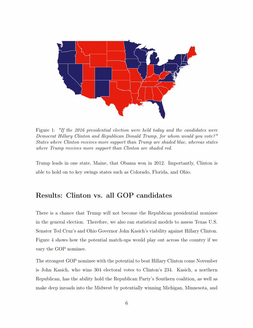
Figure 1 shows that if the election were held today, we estimate that Hillary Clinton

would win the presidency with 328 electoral votes to Donald Trump’s 210. States

where Clinton receives more support than Trump are shaded blue, whereas states

where Trump receives more support than Clinton are shaded red.

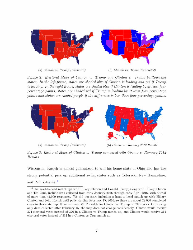
Figure 2 shows that the estimated margins between the two candidates are less than

four percentage points in Florida, Indiana, Maine, Michigan, Nevada, Ohio, and Penn-

sylvania. States such as Missouri and North Carolina appear to be safely in the Re-

publican column, wheras states in the upper Midwest such as Iowa, Minnesota and

Wisconsin appear to be leaning strongly toward the Democrats.

In the 2012 election, President Barack Obama received 332 electoral votes and former

Massachusetts Governor Mitt Romney received 206 electoral votes. Figure 3 compares

the Clinton vs. Trump estimates with results from the 2012 Presidential Election

between Barack Obama and Mitt Romney. The two maps look remarkably similar.

5

Figure 1: "If the 2016 presidential election were held today and the candidates wereDemocrat Hillary Clinton and Republican Donald Trump, for whom would you vote?"States where Clinton receives more support than Trump are shaded blue, whereas stateswhere Trump receives more support than Clinton are shaded red.

Trump leads in one state, Maine, that Obama won in 2012. Importantly, Clinton is

able to hold on to key swings states such as Colorado, Florida, and Ohio.

Results: Clinton vs. all GOP candidates

There is a chance that Trump will not become the Republican presidential nominee

in the general election. Therefore, we also ran statistical models to assess Texas U.S.

Senator Ted Cruz’s and Ohio Governor John Kasich’s viability against Hillary Clinton.

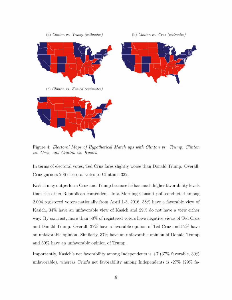
Figure 4 shows how the potential match-ups would play out across the country if we

vary the GOP nominee.

The strongest GOP nominee with the potential to beat Hillary Clinton come November

is John Kasich, who wins 304 electoral votes to Clinton’s 234. Kasich, a northern

Republican, has the ability hold the Republican Party’s Southern coalition, as well as

make deep inroads into the Midwest by potentially winning Michigan, Minnesota, and

6

(a) Clinton vs. Trump (estimated) (b) Clinton vs. Trump (estimated)

Figure 2: Electoral Maps of Clinton v. Trump and Clinton v. Trump battlegroundstates. In the left frame, states are shaded blue if Clinton is leading and red if Trumpis leading. In the right frame, states are shaded blue if Clinton is leading by at least fourpercentage points, states are shaded red if Trump is leading by at least four percentagepoints and states are shaded purple if the difference is less than four percentage points.

(a) Clinton vs. Trump (estimated) (b) Obama vs. Romney 2012 Results

Figure 3: Electoral Maps of Clinton v. Trump compared with Obama v. Romney 2012Results

Wisconsin. Kasich is almost guaranteed to win his home state of Ohio and has the

strong potential pick up additional swing states such as Colorado, New Hampshire,

and Pennsylvania.6

6The head-to-head match ups with Hillary Clinton and Donald Trump, along with Hillary Clintonand Ted Cruz, include data collected from early January 2016 through early April 2016, with a totalof more than 44,000 responses. We did not start including a head-to-head match up with HillaryClinton and John Kasich until polls starting February 15, 2016, so there are about 28,000 completedcases in this match up. If we estimate MRP models for Clinton vs. Trump or Clinton vs. Cruz usingonly data collected after February 15, the map does not change considerably. Clinton would receive324 electoral votes instead of 326 in a Clinton vs Trump match up, and Clinton would receive 314electoral votes instead of 332 in a Clinton vs Cruz match up.

7

(a) Clinton vs. Trump (estimates) (b) Clinton vs. Cruz (estimates)

(c) Clinton vs. Kasich (estimates)

Figure 4: Electoral Maps of Hypothetical Match ups with Clinton vs. Trump, Clintonvs. Cruz, and Clinton vs. Kasich

In terms of electoral votes, Ted Cruz fares slightly worse than Donald Trump. Overall,

Cruz garners 206 electoral votes to Clinton’s 332.

Kasich may outperform Cruz and Trump because he has much higher favorability levels

than the other Republican contenders. In a Morning Consult poll conducted among

2,004 registered voters nationally from April 1-3, 2016, 38% have a favorable view of

Kasich, 34% have an unfavorable view of Kasich and 29% do not have a view either

way. By contrast, more than 50% of registered voters have negative views of Ted Cruz

and Donald Trump. Overall, 37% have a favorable opinion of Ted Cruz and 52% have

an unfavorable opinion. Similarly, 37% have an unfavorable opinion of Donald Trump

and 60% have an unfavorable opinion of Trump.

Importantly, Kasich’s net favorability among Independents is +7 (37% favorable, 30%

unfavorable), whereas Cruz’s net favorability among Independents is -27% (29% fa-

8

vorable, 56% unfavorable) and Trump’s net favorability is -24% (36% favorable, 60%

unfavorable).

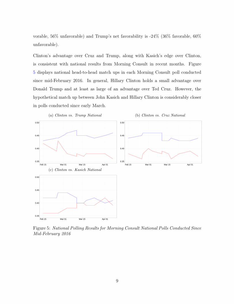
Clinton’s advantage over Cruz and Trump, along with Kasich’s edge over Clinton,

is consistent with national results from Morning Consult in recent months. Figure

5 displays national head-to-head match ups in each Morning Consult poll conducted

since mid-February 2016. In general, Hillary Clinton holds a small advantage over

Donald Trump and at least as large of an advantage over Ted Cruz. However, the

hypothetical match up between John Kasich and Hillary Clinton is considerably closer

in polls conducted since early March.

(a) Clinton vs. Trump National

0.35

0.40

0.45

0.50

Feb 15 Mar 01 Mar 15 Apr 01

(b) Clinton vs. Cruz National

0.35

0.40

0.45

0.50

Feb 15 Mar 01 Mar 15 Apr 01

(c) Clinton vs. Kasich National

0.35

0.40

0.45

0.50

Feb 15 Mar 01 Mar 15 Apr 01

Figure 5: National Polling Results for Morning Consult National Polls Conducted SinceMid-February 2016

9

Alternative Specifications

In addition to creating state-by-state estimates using MRP, we used an alternative

approach where we first allocated respondents to their respective state and then we

post-stratified by applying state-based weights using population parameters from the

2012 Current Population Survey (CPS). This approach does not utilize the state-level

grouping variables, and the estimates in this approach are more variable in states with

smaller samples.

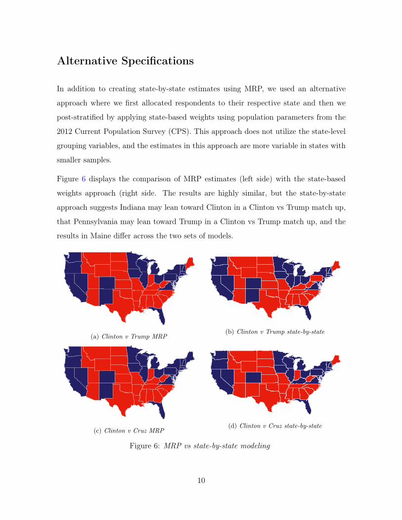
Figure 6 displays the comparison of MRP estimates (left side) with the state-based

weights approach (right side. The results are highly similar, but the state-by-state

approach suggests Indiana may lean toward Clinton in a Clinton vs Trump match up,

that Pennsylvania may lean toward Trump in a Clinton vs Trump match up, and the

results in Maine differ across the two sets of models.

(a) Clinton v Trump MRP(b) Clinton v Trump state-by-state

(c) Clinton v Cruz MRP(d) Clinton v Cruz state-by-state

Figure 6: MRP vs state-by-state modeling

10

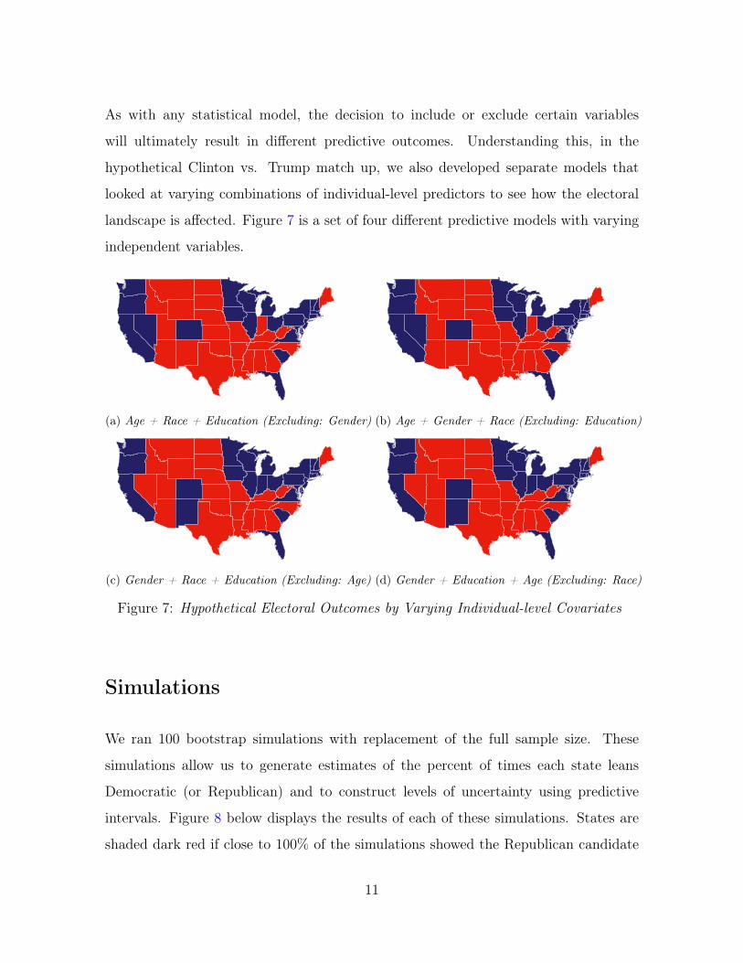
As with any statistical model, the decision to include or exclude certain variables

will ultimately result in different predictive outcomes. Understanding this, in the

hypothetical Clinton vs. Trump match up, we also developed separate models that

looked at varying combinations of individual-level predictors to see how the electoral

landscape is affected. Figure 7 is a set of four different predictive models with varying

independent variables.

(a) Age + Race + Education (Excluding: Gender) (b) Age + Gender + Race (Excluding: Education)

(c) Gender + Race + Education (Excluding: Age) (d) Gender + Education + Age (Excluding: Race)

Figure 7: Hypothetical Electoral Outcomes by Varying Individual-level Covariates

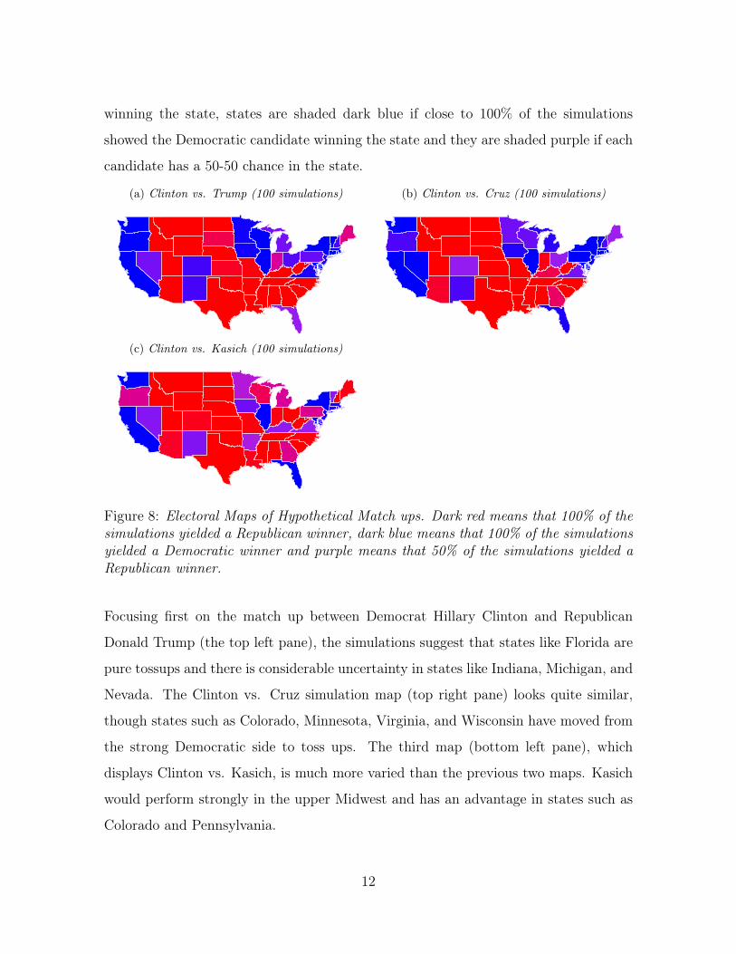
Simulations

We ran 100 bootstrap simulations with replacement of the full sample size. These

simulations allow us to generate estimates of the percent of times each state leans

Democratic (or Republican) and to construct levels of uncertainty using predictive

intervals. Figure 8 below displays the results of each of these simulations. States are

shaded dark red if close to 100% of the simulations showed the Republican candidate

11

winning the state, states are shaded dark blue if close to 100% of the simulations

showed the Democratic candidate winning the state and they are shaded purple if each

candidate has a 50-50 chance in the state.

(a) Clinton vs. Trump (100 simulations) (b) Clinton vs. Cruz (100 simulations)

(c) Clinton vs. Kasich (100 simulations)

Figure 8: Electoral Maps of Hypothetical Match ups. Dark red means that 100% of thesimulations yielded a Republican winner, dark blue means that 100% of the simulationsyielded a Democratic winner and purple means that 50% of the simulations yielded aRepublican winner.

Focusing first on the match up between Democrat Hillary Clinton and Republican

Donald Trump (the top left pane), the simulations suggest that states like Florida are

pure tossups and there is considerable uncertainty in states like Indiana, Michigan, and

Nevada. The Clinton vs. Cruz simulation map (top right pane) looks quite similar,

though states such as Colorado, Minnesota, Virginia, and Wisconsin have moved from

the strong Democratic side to toss ups. The third map (bottom left pane), which

displays Clinton vs. Kasich, is much more varied than the previous two maps. Kasich

would perform strongly in the upper Midwest and has an advantage in states such as

Colorado and Pennsylvania.

12

Some caveats in this work

In this section, we describe a few caveats concerning MRP in particular and in con-

structing state-level estimates more broadly.

First, we interviewed registered voters nationally rather than likely voters. Only about

eight in 10 registered voters actually voted in the 2012 Presidential election, according

to the 2012 Current Population Survey.7 If the composition of registered voters and

likely voters differs considerably, then our results may change.

Second, respondents on these national surveys were asked about their vote if the elec-

tion were held today. The November election is more than six months away and much

can change throughout the Spring, Summer and Fall.

Third, we include all interviews conducted since January 1, 2016 for our estimates

of Clinton vs. Trump and Clinton vs. Cruz. However, more than 30 primaries and

caucuses have been held this cycle and a significant number of Americans may have

changed their minds over the course of the past three months. It is worth noting that

the estimates look similar if we construct them based only on interviews from late Mid-

February 2016 through the present rather than starting in early January 2016.

Fourth, our poststratification utilizes 5-year estimates from the American Community

Survey (ACS) among a sample of adult citizens. Using this set of data allows us to

include variables such as education and race in our modeling that might not be available

in statewide voter files, but it contains a broader universe of adults than registered voter

samples from voter files might include. If likely voters differ considerably from likely

voters based on characteristics such as age, gender and education, then our estimates

may be biased.

Fifth, about one in six registered voters are undecided, or say they do not have an7Link to the voting supplement of the November 2012 Current Population Survey https://www.

census.gov/hhes/www/socdemo/voting/publications/p20/2012/tables.html

13

opinion either way, across the three hypothetical match ups. In this draft, we do not

model how these undecided voters might act if they had to take a position.

Sixth, as shown above, the MRP models can be sensitive to the inclusion or exclusion

of additional individual level and state-level variables, especially in smaller states or in

battleground states.

Conclusions

Morning Consult asked more than 44,000 registered voters nationally over the past

three months who they would support in a series of hypothetical general election match

ups. We used a statistical technique called multilevel regression and poststratification

(MRP) to construct state-level estimates from the national survey data. The results

suggest that Democrat Hillary Clinton currently has an advantage over Republicans

Donald Trump and Ted Cruz. On the other hand, the estimates suggest that Ohio

Governor John Kasich edges out Clinton, likely due to much higher favorability levels

among registered voters than Trump or Cruz and advantages in his home state of Ohio.

Many caveats are in store due to the length of time between now and November, the

high proportion of adults who are undecided and close margins in key states such as

Florida, but the results suggest the 2016 presidential election map will look similar to

the 2012 map if Democrat Hillary Clinton and Republican Donald Trump are their

parties’ respective nominees.

14

References

Fair, Ray C. 1978. “The effect of economic events on votes for president.” The Review

of Economics and Statistics pp. 159–173.

Gelman, Andrew. 2009. Red state, blue state, rich state, poor state: Why Americans

vote the way they do. Princeton University Press.

Gelman, Andrew, and Jennifer Hill. 2006. Data analysis using regression and multi-

level/hierarchical models. Cambridge University Press.

Ghitza, Yair, and Andrew Gelman. 2013. “Deep interactions with MRP: Election

turnout and voting patterns among small electoral subgroups.” American Journal of

Political Science 57(3): 762–776.

Howe, Peter D., Matto Mildenberger, Jennifer R. Marlon, and Anthony Leiserowitz.

2015. “Geographic variation in opinions on climate change at state and local scales

in the USA.” Nature Climate Change 5(6): 596–603.

Kastellec, Jonathan P., Jeffrey R. Lax, and Justin Phillips. 2010. “Estimating state

public opinion with multi-level regression and poststratification using R.” Unpub-

lished manuscript, Princeton University .

Lax, Jeffrey R., and Justin H. Phillips. 2009. “How should we estimate public opinion

in the states?” American Journal of Political Science 53(1): 107–121.

Leemann, Lucas, and Fabio Wasserfallen. 2014. “Extending the Use and Prediction

Precision of Subnational Public Opinion Estimation.” Unpublished Manuscript .

Park, David K., Andrew Gelman, and Joseph Bafumi. 2004. “Bayesian multilevel

estimation with poststratification: state-level estimates from national polls.” Political

Analysis 12(4): 375–385.

Warshaw, Christopher, and Jonathan Rodden. 2012. “How should we measure district-

level public opinion on individual issues?” The Journal of Politics 74(01): 203–219.

15

Appendices

Model Specifications

Below we describe the specific parameters in our MRP model.

Let Y be defined as the predicted probability that any one individual will supportHillary Clinton

Pr(yi = 1) = Y = logit−1(B0 + αagek[i] + αeducation

l[i] + αgenderm[i] + αstate

s[i] +Bxi)

Where:

logit−1(α) =exp(α)

exp(α) + 1

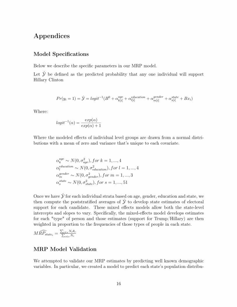
Where the modeled effects of individual level groups are drawn from a normal distri-butions with a mean of zero and variance that’s unique to each covariate.

αagek ∼ N(0, σ2

age), for k = 1, ..., 4

αeducationl ∼ N(0, σ2

education), for l = 1, ..., 4

αgenderm ∼ N(0, σ2

gender), for m = 1, ..., 3

αstates ∼ N(0, σ2

state), for s = 1, ..., 51

Once we have Y for each individual strata based on age, gender, education and state, wethen compute the poststratified averages of Y to develop state estimates of electoralsupport for each candidate. These mixed effects models allow both the state-levelintercepts and slopes to vary. Specifically, the mixed-effects model develops estimatesfor each "type" of person and those estimates (support for Trump/Hillary) are thenweighted in proportion to the frequencies of those types of people in each state.MRPstatei =

∑c∈s Ncθc∑c∈s Nc

MRP Model Validation

We attempted to validate our MRP estimates by predicting well known demographicvariables. In particular, we created a model to predict each state’s population distribu-

16

tion by gender. The same variables that were used to predict election outcomes wereused in the validation model (minus gender).

We then compared the MRP-gender-model to the standard approach of allocatingrespondents by state and applying state-based weights to see which method producedless error in predicting known census quantities of gender distributions by state.

To compare each method (MRP vs state-aggregation) we calculated the root-mean-squared-error (RMSE) for each method. RMSE is used to measure of the total dif-ferences between values predicted by the MRP model and the true observed values(Census estimates of gender by state). A lower RMSE score indicates a more accuratepredictive model.

MRP-RMSE State-Weights-RMSE0.066 0.075

Table 1: Validation: RMSE scores for MRP and State-Weighting

When comparing MRP to the state-weights approach, we find that the RMSE for MRPis lower, which indicates that MRP performs better at predicting gender distributionsat the state level.

17