Estimating net ideal cycle time for body-in-whiteproduction lines
WC Grobler∗ DJ Kotze† JW Joubert‡
Received: 3 August 2020; Revised: 2 June 2021; Accepted: 2 June 2021
AbstractIn the automotive industry, a Body-in-White (BIW) refers to the first step, the basic structure,in the production of a vehicle. Once a BIW production line has been built, the (maximum)capacity is fixed and throughput is therefore limited by the equipment specified during thedesign phase. The main metric used to inform the production line design is the Net IdealCycle Time (NICT). Unfortunately the state of practice to estimate the NICT is a basicheuristic that does not account for production variation. In this paper we challenge thecurrent estimation approach by proposing an alternative that assumes actual production tofollow a Weibull distribution. The proposed model is derived and estimated from empiricaldata. The results suggest that BIW production lines have traditionally been designed withtoo low a capacity, resulting in planned throughput rarely being achieved. On the otherhand, increasing the design capacity implies higher initial investment. In this paper it isdemonstrated that the higher investment required is offset by reduced losses, resulting inmore reliable planning and returns.
Key words: Automotive industry, design of production systems, capacity planning, investment
appraisal, cycle time estimation, body-in-white.
1 Introduction
The BIW production line in the automotive manufacturing industry is responsible forcreating the basic structure of a vehicle. Figure 1 illustrates, through an explosion diagram,the basic structure of the BIW.
The assembly stations along the production line are typically heavily equipped with roboticwelders and automated material handling technology. In this paper the term ‘BIW’ will
∗Department of Industrial and Systems Engineering, BMW South Africa, Rosslyn, Pretoria, SouthAfrica, email: [email protected]
†Department of Industrial and Systems Engineering, BMW South Africa, Rosslyn, Pretoria, SouthAfrica, email: [email protected]
‡Corresponding author: Centre for Transport Development, Industrial & Systems Engineering,University of Pretoria, South Africa, email: [email protected]
Figure 1: Body-in-White (BIW) structure of 2012 BMW 3 series
mainly refer to the production line and not to the vehicle structure, unless explicitly statedotherwise.
Designing the BIW line is generally a complex and challenging task. The equipmentselection is subject to the required throughput and, once installed, essentially becomes theceiling for production. Production line designers use the NICT as the reference to specifyequipment capacity, which, in turn, is informed by two important design parameters. Thefirst is Takt Time (TT), the average time between the start of production of one unit andthe start of production for the next, subsequent unit and, secondly, the Overall EquipmentEfficiency (OEE).
If the NICT is short, as is the case in a fast production line, then more robots or peopleare required to complete a process step. When the NICT is longer, fewer robots or peopleare required and, consequently, results in lower financial investment. It is for this reasonthat the NICT of a (BIW) production line must be reliable. Too high an estimate resultsin inefficient use of capital, while too low an estimate means actual production cannotmeet the set targets.
In the current literature we distinguish between two streams of cycle time research. Cycletime estimation is the focus of this project and deals with the design or pre-productionstages of the line’s lifecycle [3]. Cycle time optimisation, on the other hand, deals withanalyses of and methods to improve the cycle time of a system that is already in aseries-production stage.
Although much research has been done in the semiconductor industry with regards tocycle time estimation, the state of practice in the majority of industries rely on fairly
Estimating net ideal cycle time for body-in-white production lines 3
basic heuristics. Production variation is not accounted for other than through a scalar,average safety factor like OEE.
This paper contributes to the body of knowledge by proposing a new NICT estimate, onethat takes production variation into account. The proposed model is derived from studyingempirical production data over a multi-year period in the automotive BIW environment.The analyses suggest that actual production follows a Weibull distribution, where theshape parameter can be estimated from historical data, and the scale parameter is usedto estimate the NICT.
We show that the NICT, when estimated using traditional approaches, leads to aproduction line that consistently suffers from under-performance. Consequently, expensiveproduction losses are incurred. The proposed estimate requires lines to be designed with aslightly higher capacity. Although this implies higher initial investment, we demonstrate inthis paper that the increased investment is offset by reduced losses. A direct consequence isthat production planning is more realistic, and performance of the lines are more reliable.
The remainder of this paper is arranged as follows. In the next section we review currentliterature in cycle time estimation and optimisation. In Section 3 we explore the currentstate-of-practice NICT estimation method, and demonstrate it’s limitation for designengineers. In Section 4 we study the throughput distribution of a real BIW production line.We fit an appropriate throughput distribution from empirical data over the 2012–2015period, and lay the foundation for the proposed NICT estimation. The Weibull-basedestimation approach is proposed in Section 5, and in Section 6 a comparative benchmarkis done to evaluate the feasibility of the proposed method in terms of costs. The paper isconcluded in Section 7 along with a brief research agenda.
2 Cycle time estimation and optimisation
Cycle time estimation is important in various industries. There has been a significantamount of research completed within the semi-conductor industry, with popular estimationtechniques being statistical modelling [10, 13], heuristics [1, 18], aggregation [14] andhistoric correlation approaches [2, 5, 7]. The goal of these research contributions areto develop models that could estimate the cycle time of series-production systems. Theestimation aims to get a handle on predictable production output, and then compare thesystem performance against customer demand.
More general production systems have seen fewer research contributions. Xu et al. [15]focus their research on cycle time estimation for unreliable production lines. The researchdoes not state for which industry this specific estimation is valid, but specifies that thetype of production lines under investigation are multiple product production lines. Thestudy is related to BIW production lines in terms of the unreliability of the productionlines. In their research they use chance constraint and fuzzy linear programming to predictproduction cycle time so that they can calculate production line efficiency. The main modelutilised for this is the one from Johri [8]. Presented in 1987, this linear programming modelis used to calculate the capacity of deterministic production lines of various products.
4 WC Grobler, DJ Kotze & JW Joubert
In Yang et al. [16] the focus of research falls on the relationship between cycle time andproduction throughput. Again there is no reference to the specific industry. They suggestthat the cycle time-throughput percentile of the production system could be used forstrategic planning purposes. The main assumption for their research is the use of thegeneralised gamma distribution to represent actual cycle time. Simulation is then used asan evaluation method to support their theory.
Chen & Zhou [3] propose quantile regression as an alternative method for cycle timeestimation. They start by defining the relationship between cycle time quantiles andsystem throughput. One nice approach in their method is the comparison to actual datafrom a case study to show the correlation between real data and estimation data. Thereare two major assumptions used in their work: the assumption of stationary processconvergence, and process mixing, which are based on the theory of queuing system analysis.Process mixing is not relevant for BIW production lines as the series-production setupfocuses on a single product, albeit with some minor variations between models.
In their research, Muller et al. [9] assist engineers with a tool to predict robot performancein the packaging industry. Since BIW lines also rely heavily on robots, this researchis considered relevant. The method used for robot cycle time estimation is regressionanalysis. The result is a new software tool, however, it is limited to ABB robot applicationsonly. The motivation for this study originated from a use case, and the main aim is toassist sales engineers with a tool that can give accurate production information aboutpacking robots to potential clients specific to their industry.
There is a lack of research surrounding BIW production lines, and particularly arounddesign topics such as NICT estimation.
3 State of practice
The current method to estimate NICT for a BIW production line starts by calculating theTakt Time (TT), expressed in seconds;
TT =NAT
MTT, (1)
where Mean Throughput Target (MTT) is expressed in units per hour (uph), and NetAvailable Time (NAT). The NAT is typically assumed to be 3600 seconds per hour.
NICT, in turn, is calculated from talk time and the Overall Equipment Efficiency (OEE)[12];
NICT =OEE ×NAT
MTT= TT ×OEE. (2)
Consider for example a BIW line that is planned to achieve, on average, a throughput ofMTT = 15 uph. We use 15 uph as it is aligned with the planned capacity of the line we willuse for empirical data later. In the automotive industry an OEE = 0.85 is considered best
Estimating net ideal cycle time for body-in-white production lines 5
Figure 2: The throughput distribution of a BIW production line fitted into a normal distributionusing the three-sigma rule as a starting point.
practice and used in the calculation. The result, when substituting these values into (1)and (2), is an ideal cycle time of
NICT =3600× 0.85
15= 204 s,
or expressed otherwise, a mean throughput of 17.65 uph. This cycle time value is thenused as an input into specifying equipment and designing the line capacity.
At the same time line designers account for production variation by subscribing, possiblyunconsciously, to the idea that the actual throughput of the production line will followa normal distribution. More specifically, that under normal production conditions for aline that is under control the average throughput will be within three standard deviationsabove and below the mean.
P{µ− 3σ < X < µ+ 3σ} = 0.9973. (3)
This is graphically represented in Figure 2. For this to be true, using the example ofa 15 uph line, the standard deviation for actual throughput should be a very ambitious0.95 uph.
Since the NICT is used to inform equipment decisions, it essentially becomes thethroughput ceiling, and we refer to the throughput associated with the NICT as the Upper
6 WC Grobler, DJ Kotze & JW Joubert
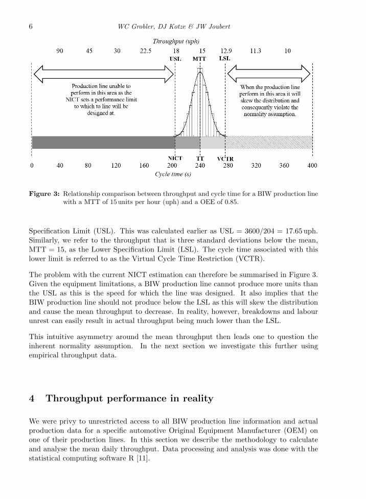
Figure 3: Relationship comparison between throughput and cycle time for a BIW production linewith a MTT of 15 units per hour (uph) and a OEE of 0.85.
Specification Limit (USL). This was calculated earlier as USL = 3600/204 = 17.65 uph.Similarly, we refer to the throughput that is three standard deviations below the mean,MTT = 15, as the Lower Specification Limit (LSL). The cycle time associated with thislower limit is referred to as the Virtual Cycle Time Restriction (VCTR).
The problem with the current NICT estimation can therefore be summarised in Figure 3.Given the equipment limitations, a BIW production line cannot produce more units thanthe USL as this is the speed for which the line was designed. It also implies that theBIW production line should not produce below the LSL as this will skew the distributionand cause the mean throughput to decrease. In reality, however, breakdowns and labourunrest can easily result in actual throughput being much lower than the LSL.
This intuitive asymmetry around the mean throughput then leads one to question theinherent normality assumption. In the next section we investigate this further usingempirical throughput data.
4 Throughput performance in reality
We were privy to unrestricted access to all BIW production line information and actualproduction data for a specific automotive Original Equipment Manufacturer (OEM) onone of their production lines. In this section we describe the methodology to calculateand analyse the mean daily throughput. Data processing and analysis was done with thestatistical computing software R [11].
Estimating net ideal cycle time for body-in-white production lines 7
4.1 Methodology
We extracted data for the period 2012–2015. Every unit that is produced triggers anincremental counter, in real time, in the central database. At the end of each day thedate, the number of shifts for that day, the total number of units produced, and the day’svolume target is recorded.
From this we calculate the Mean Throughput (MT);
MT =TDV
DHW,
where MT is expressed in uph, Total Daily Volume (TDV) is the total daily number ofunits (volume) that was produced and Daily Hours Worked (DHW) is the total numberof hours worked per specific day. With standard 8-hour shifts this would typically just beeight times the number of shifts for the day.
Practical experience and management input suggested that the daily throughput isdependent on the day of the week. There is typically higher absenteeism of employeeson Mondays, Fridays and Saturdays, while labour productivity is also lower on these days.Production on Sundays deviates as well, but this is due to operational changes being testedon the production line on Sundays. These daily variations were confirmed in the empiricaldata and is illustrated in Figure 4.
Figure 4: The distribution of daily Mean Throughput (MT) for the years 2012–2015 as a functionof the day of the week.
Such variations is, at least partially, under management’s control. Since we want to usethe throughput data to estimate and inform future design calculations in the NICT, weremoved Mondays, Fridays, Saturdays and Sundays.
8 WC Grobler, DJ Kotze & JW Joubert
The resulting data for the remaining three days were combined. The mean throughput foreach production year was plotted in the histograms of Figure 5. The normal distribution
(a) 2012 (b) 2013
(c) 2014 (d) 2015
Figure 5: The empirical Mean Throughput (MT) distribution, expressed in uph, for the period2012–2015.
in each histogram represents a comparative reference to the planned throughput for a lineof the same capacity, 15 uph. The assumption of the comparative reference is in line withour earlier discussion of the state of practice: a) actual output would be within threestandard deviations of the MTT of 15 uph; and b) the standard deviation for the line isσ = 0.95 uph.
Three observations are worth making at this point. Firstly, we see that the empirical datawas never distributed within the limits of the LSL and USL. Secondly, the throughputdistribution does not appear to be normally distributed, and is consistently left-skewed.This is in line with the earlier argument that the USL acts as a production ceiling, whilelower-than-limit production is indeed possible. Thirdly, there is a noticable differencebetween 2012 and the other years in terms of the long left tail. This performance
Estimating net ideal cycle time for body-in-white production lines 9
difference is a result of 2012 being the launch year of a new product. In the launchyear performance is gradually increased from a very low throughput base. It usually takesthe BIW production line about six months from start of production to mature before theline reaches its maximum performance.
4.2 Empirical throughput performance
To identify an appropriate distribution we start by giving some summary statistics abouteach year’s throughput data in Table 1.
Table 1: Summary statistics for the empirical throughput: 2012–2015.
The actual standard deviation, for each year, is much higher that the required σ = 0.95for the values to fall within three standard deviations around the mean.
The sample skewness is a measure of the data’s asymmetry about its mean. Negativevalues is indicative of a skewed distribution. In all cases the value is significantly differentfrom zero, confirming that the data is not symmetric around the mean. The kurtosis metricis a measure of the heavy-tailedness of the distribution of the data. Higher kurtosis meansmore of the variance is the result of infrequent extreme observations, as opposed to morefrequent but modestly sized deviations. A kurtosis value of less than 3 (2014) suggeststhat the distribution is platykurtic, meaning there are fewer and less extreme outliers thanwhat one might find in a normal distribution with the same mean and standard deviation.In a quality assurance sense, this could be indicative of a production line that is ‘undercontrol’. For the other three years the kurtosis values exceed 3 suggesting the distributionsare leptokurtic and contain more outliers than one would find in a corresponding normaldistribution.
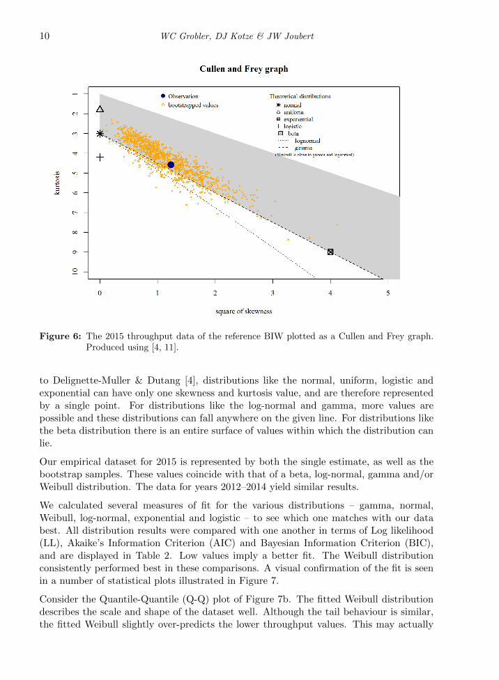
We used the fitdistrplus package in R [4] and prepared a Cullen and Frey graph toidentify other possible distributions that could potentially fit the empirical data better. Fora number of common distributions, the graph indicates the range of skewness and kurtosisvalues associated with that distribution. However, because skewness and kurtosis are notrobust statistics, we take the uncertainty of the estimated values of kurtosis and skewnessinto account. A non-parametric bootstrap procedure, based on Efron & Tibshirani [6], isperformed. Values of skewness and kurtosis are computed on bootstrap samples: drawingrandom samples with replacement from the original data set. The resulting estimates forthe 2015 data set is given in Figure 6.
The Cullen and Frey reference graph consists out of points, lines and surfaces. According
10 WC Grobler, DJ Kotze & JW Joubert
Figure 6: The 2015 throughput data of the reference BIW plotted as a Cullen and Frey graph.Produced using [4, 11].
to Delignette-Muller & Dutang [4], distributions like the normal, uniform, logistic andexponential can have only one skewness and kurtosis value, and are therefore representedby a single point. For distributions like the log-normal and gamma, more values arepossible and these distributions can fall anywhere on the given line. For distributions likethe beta distribution there is an entire surface of values within which the distribution canlie.
Our empirical dataset for 2015 is represented by both the single estimate, as well as thebootstrap samples. These values coincide with that of a beta, log-normal, gamma and/orWeibull distribution. The data for years 2012–2014 yield similar results.
We calculated several measures of fit for the various distributions – gamma, normal,Weibull, log-normal, exponential and logistic – to see which one matches with our databest. All distribution results were compared with one another in terms of Log likelihood(LL), Akaike’s Information Criterion (AIC) and Bayesian Information Criterion (BIC),and are displayed in Table 2. Low values imply a better fit. The Weibull distributionconsistently performed best in these comparisons. A visual confirmation of the fit is seenin a number of statistical plots illustrated in Figure 7.
Consider the Quantile-Quantile (Q-Q) plot of Figure 7b. The fitted Weibull distributiondescribes the scale and shape of the dataset well. Although the tail behaviour is similar,the fitted Weibull slightly over-predicts the lower throughput values. This may actually
Estimating net ideal cycle time for body-in-white production lines 11
Table 2: Distribution fit results for all data (2012–2015) using various test distributions.
(a) Histogram and theoretical densities (b) Q-Q plot
(c) Empirical and theoretical CDFs (d) P-P plot
Figure 7: The 2015 throughput data of the reference BIW compared to a theoretical throughputof a Weibull distribution.
be to our benefit as it means we will provide a conservative estimate for the NICT. Theover-prediction of low-throughput instances is confirmed in the higher probabilities in theProbability-Probability (P-P) plot of Figure 7d.
The current NICT estimation method does not make an explicit assumption that the MTof a BIW production line is normally distributed, but it assumes that the performancecharacteristics of all production lines are similar. As a result, the current estimator ignoresany possible past performance of a production line, or industry experience. Instead, wecan now propose an estimator that uses our knowledge of past performance.
12 WC Grobler, DJ Kotze & JW Joubert
5 Estimating NICT using a Weibull distribution
A Weibull distribution is described using two parameters: shape (k) and scale (λ). Theempirical data gives us a good idea of what the shape parameter must be. The scale,however, can be left as an input parameter for the designer to determine the NICT so thatthe actual MTT can be achieved.
The shape of the distribution can be estimated by taking the mean shape for all theempirical years, excluding 2012. The data from 2012 was omitted since the launch-year isa valid assignable cause. By omitting 2012’s shape parameter, the mean shape is increasedfrom k ≈ 9.58 to k ≈ 11.17, and at the same time the standard deviation of these estimatesis reduced from kσ ≈ 2.77 to kσ ≈ 0.37.
Given the mean, µ, the Weibull distribution’s scale parameter, λ, can be calculated usingthe relation
µ = λΓ(1 + 1/k), (4)
where Γ is the gamma function and k is the (estimated) shape parameter, k, of the Weibulldistribution, see [17]. The gamma function is an extension of the factorial function andcan be expressed as
Γ(x) =
∫ ∞0
zx−1e−zdz,
where x is positive. The estimated standard deviation for the Weibull distribution, σ, canbe calculated using
σ2 = λ2[Γ(1 + 2/k)− Γ(1 + 1/k)2]. (5)
The calculated standard deviation can be compared to the empirical data reported inTable 1. The USL is related to the quantile function, or the inverse cumulative distribution;
USL = λ[−ln(1− p)]1k .
For a given probability p the quantile function provides a value (mean throughput in thiscase) such that the random variable (throughput) is less than or equal to this value withprobability p. Knowing p we can calculate the NICT;
NICT =NAT
λ[−ln(1− p)]1k
,
where NAT is again 3 600 s. The value of p could be considered the required certainty withwhich BIW line designers want to estimate the NICT. Consider the earlier discussion whereline designers assume the three-sigma rule, p = 0.9973. That is, 99.73% of all observationsshould fall below the USL.
Estimating net ideal cycle time for body-in-white production lines 13
6 Discussion of results
In this section we apply our proposed Weibull-based method to the example line witha MTT of 15 uph. From the empirical data of 2013–2015 we use a shape parameter ofk = 11.17. Using (4) we calculate the scale parameter as λ = 15.53, and using (5) wecalculate σ = 1.61. This is quite close the the mean empirical standard deviation ofσ = 1.69.
The final step is estimating that NICT ≈ 197.67 s and the associated USL ≈ 18.21 uph.This is a 3.2% increase in throughput over the NICT when using the current, traditionalmethod. Consequently, one can expected an approximate increase of 3% in financialinvestment as well, to account for higher capacity equipment requirements.
A total of 10 different BIW investment projects were analysed to determine an averageinvestment figure as well as an average loss per unit from the production program. Thisinformation was again supplied by the reference OEM. In the following example we scaledthe real figures to protect the confidentiality of investment and loses figures of the specificOEM.
Consider a new BIW production line where 3.25 Million Euros are required per unit perhour to achieve the required MTT. For every one unit that is lost from the productionprogram, there is a 2,000 Euro income loss for the specific production facility. This canquickly result in a negative business case if the daily income is surpassed by the daily fixedand running costs. This means that for a BIW production line with a planned MTT of15 uph, the required investment would be 48.75 Million Euro using the current method,and 50.26 Million Euro for our proposed method. This is an increase of 1.51 Million Euro,or approximately 3.1%.
Over the 7 year production lifecycle, and using the empirical data, we can calculate thatthe expected losses would total 1 646 units due to unforeseen process variations that arenot catered for by the current NICT estimation method. The 1 646 units loss equates toa monetary loss of 3.24 Million Euro over the production life cycle.
This means that using the proposed method instead of the current method, the total losscan be reduced by almost 50% in monetary terms. The proposed method covers in ourcase four years of real production history. Included in this history is unforeseen eventssuch as strikes, major power outages and various other variantions that are not considerwhen defining NICT. The Weibull estimate honours the production ceiling, as well as theleft-skewed distribution observed in empirical data.
7 Conclusion
Analysing empirical data of a real BIW production line, we can conclude that the meandaily throughput follows a Weibull distribution. We propose a new method to estimateNICT based on this distribution.
Our proposed method has a number of advantages over the current method used forestimating NICT. Firstly, the Weibull-based method is more representative of the real
14 WC Grobler, DJ Kotze & JW Joubert
production characteristics and behaviour of the automotive BIW production lines. Thisallows for more realistic and reliable planning. However, this approach requires historicalproduction data for the specific line considered or a similar line.
Secondly, knowing the Weibull distribution parameters allow a more vivid capability targetfor performance measurement and control. Our new method resulted in a 3.1% increasein estimated NICT, which will be different for every BIW production line.
In the illustrative example we noted a 3.2% increase in the estimated cycle time, whichwould equate to a probable investment increase of a similar magnitude to compensatefor the faster production line. The increase in investment can be justified (or rejected)by comparing it to the expected losses due to variation of the relevant BIW productionline, and it is proposed that a simple business case can determine if the extra financialinvestment outweighs the expected production losses.
Our study focused purely on one specific BIW production line where only one variant isproduced. There are production lines where two or even three automotive product variantsare produced. These lines are more complex but should yield similar results. It is proposedto not only investigate these multiple variant production lines, but also production lineswhere higher throughputs are applicable, for example 45 uph lines. It would be engrossingto see what shape and scale other BIW production lines exhibit, and if there are any shapeor scale correlations between these different throughput lines. Further research is proposedwith focus on other manufacturing industries where NICT is also used as a productionline design input.
References[1] Akhavan-Tabatabaei R, Ding S & Shanthikumar JG, 2009, A method for cycle time estimation
of semiconductor manufacturing toolsets with correlations, Proceedings of the 2009 Winter SimulationConference (WSC), Austin (TX), pp. 1719–1729.
[2] Akhavan-Tabatabaei R, Ucros JJ & Shanthikumar GJ, 2010, Application of Erlang distributionin cycle time estimation of toolsets with WIP-Dependant arrival and service in a single product-typesingle failure-type environment, Proceedings of the 2010 Winter Simulation Conference, Baltimore(MD), pp. 2531–2540.
[3] Chen N & Zhou S, 2011, Simulation-based estimation of cycle time using quantile regression, IIETransactions, 43(3), pp. 176–191.
[4] Delignette-Muller ML & Dutang C, 2015, fitdistrplus: An R Package for fitting distributions,Journal of Statistical Software, 64(4), pp. 1–34.
[5] Delp D, Si J & Fowler JW, 2006, The development of the complete X-Factor contributionmeasurement for improving cycle time and cycle time variability, IEEE Transactions on SemiconductorManufacturing, 19(3), pp. 352–362.
[6] Efron B & Tibshirani RJ, 1994, An Introduction to the Bootstrap, CRC Press, Boca Raton (FL).
[7] Huang HP, Yeh CF, Juang JY, Lin LR & Chen T, 1998, Dynamic average method for cycle timeestimator in an IC fab, 1998 Semiconductor Manufacturing Technology Workshop, Hsinchu.
[8] Johri PK, 1987, A linear programming approach to capacity estimation of automated production lineswith finite buffers, International Journal of Production Research, 25(6), pp. 851–866.
Estimating net ideal cycle time for body-in-white production lines 15
[9] Muller M, Kuhlenkotter B & Geiger H, 2014, Cycle time estimation for a delta-type robot,41st Symposium on Robotics, Munich, pp. 225–231.
[10] Pearn WL, Tai YT & Lee JH, 2009, Statistical approach for cycle time estimation in semiconductorpackaging factories, IEEE Transactions on Electronics Packaging Manufacturing, 32(3), pp. 198–205.
[11] R Development Core Team, 2016, R: A language and environment for statistical computing.
[12] Stamatis DH, 2010, The OEE primer — Understanding Overall Equipment Effectiveness, CRCPress, New York (NY).
[13] Tai YT, Pearn WL & Lee JH, 2012, Cycle time estimation for semiconductor final testing processeswith Weibull-distributed waiting time, International Journal of Production Research, 50(2), pp.581–592.
[14] Veeger CPL, Etman LFP, Van Herk J & Rooda JE, 2009, Predicting the mean cycle timeas a function of throughput and product mix for cluster tool workstations using EPT-based aggregatemodeling, pp. 80–85.
[15] Xu M, Abdul-Kader W & Ganjavi O, 2009, Cycle time estimation of a multiple product productionline: An approach with fuzzy and chance-constrained programming, Infor, 47(2), pp. 93–103.
[16] Yang F, Ankenman BE & Nelson BL, 2005, Estimation of percentiles of cycle time inmanufacturing simulation. Proceedings of the 2005 Winter Simulation Conference (WSC), Orlando(FL), pp. 475–484
[17] Yang G, 2007, Life Cycle Reliability Engineering, John Wiley & Sons, New York (NY).
[18] Zhou Z & Rose O, 2013, Cycle time variance minimization for WIP balance approaches in waferfabs, Proceedings of the 2013 Winter Simulation Conference, Washington (DC), pp. 3777–3788.