70
Fabio Ricciato, Peter Widhalm, Massimo Craglia and Francesco Pantisano 2015 Estimating population density distribution from network-based mobile phone data Report EUR 27361 EN
Fabio Ricciato, Peter Widhalm, Massimo Craglia and Francesco Pantisano
2015
Estimating population density distribution from network-based mobile phone data
Report EUR 27361 EN

European Commission
Joint Research Centre
Institute for Environment and Sustainability
Contact information
Dr. Massimo Craglia
Address: Joint Research Centre, Via Enrico Fermi 2749, TP 262, 21027 Ispra (VA), Italy
E-mail: [email protected]
Tel.: +39 0332 78 6269
JRC Science Hub
https://ec.europa.eu/jrc
Legal Notice
This publication is a Technical Report by the Joint Research Centre, the European Commission’s in-house science service. It
aims to provide evidence-based scientific support to the European policy-making process. The scientific output expressed
does not imply a policy position of the European Commission. Neither the European Commission nor any person acting on
behalf of the Commission is responsible for the use which might be made of this publication.
JRC96568
EUR 27361 EN
ISBN 978-92-79-50193-7 (PDF)
ISSN 1831-9424 (online)
doi:10.2788/162414
Luxembourg: Publications Office of the European Union, 2015
© European Union, 2015
Reproduction is authorised provided the source is acknowledged.
Abstract
In this study we address the problem of leveraging mobile phone network-based data for the task of estimating
population density distribution at pan-European level. The primary goal is to develop a methodological framework for the
collection and processing of network-based data that can be plausibly applied across multiple Mobile Network Operators
(MNOs). The proposed method exploits more extensive network topology information than is considered in most state-of-
the-art literature, i.e., (approximate) knowledge of cell coverage areas is assumed instead of merely cell tower locations. A
distinguishing feature of the proposed methodology is the capability of taking as input a combination of cell-level and
Location Area-level data, thus enabling the integration of data from Call Detail Records (CDR) with other network-based
data sources, e.g., Visitor Location Register (VLR). Different scenarios are considered in terms of input data availability at
individual MNOs (CDR only, VLR only, combinations of CDR and VLR) and for multi-MNO data fusion, and the relevant
tradeoff dimensions are discussed. At the core of the proposed method lies a novel formulation of the population
distribution estimation as a Maximum Likelihood estimation problem. The proposed estimation method is validated for
consistency with artificially- generated data in a simplified simulation scenario. Final considerations are provided as input
for a future pilot study validating the proposed methodology on real-world data.
Extraction of population density distribution fromnetwork-based mobile phone data
Fabio Ricciato1, Pete Widhalm2, Massimo Craglia3 and Francesco Pantisano3.
July 29, 2015
1Fabio Ricciato is with the University of Ljublijana, Faculty of Computer and Information Science, Ljubli-jana, Slovenia, and with the Austrian Institute of Technology (AIT), Mobility Department, Vienna, Austria.Email: [email protected]
2Peter Widhalm is with the Austrian Institute of Technology (AIT), Mobility Department, Vienna. [email protected]
3Massimo Craglia and Francesco Pantisano are with the Institute for Environment and Sustainabilityof the Joint Research Centre (JRC), European Commission, Ispra, Italy. Email: massimo.craglia,
Executive Summary
The vast majority of people nowadays carries (at least) a mobile phone, and every mobile phoneis logically “attached” to the network infrastructure of a Mobile Network Operator (MNO). TheMNO infrastructure is composed of multiple radio “cells” of different size — ranging from tens ofmeters up to several kilometers — and at any time the phone is logically “camped” to one cell.Upon certain events — e.g., when initiating or receiving a phone call or SMS — the mobile phonereveals its current cell location to the network, and the latter stores this information (permanently)in the so-called Call Detail Record (CDR) database for billing purposes. Moreover, radio cellsare hierarchically organised into larger spatial entities called Location Areas (LAs): whenever thephone moves from one LA to another, it informs the network, and the latter stores this informa-tion (temporarily) in the so-called Visitor Location Register (VLR) as a routine network operation.Therefore, both types of network-based data, CDR and VLR, embed information about the loca-tion of every mobile phone at the level of radio cells and/or LAs. Several research work in the lastdecade has shown that, in principle, it is possible to leverage network-based data from MNO toinfer human mobility patterns (e.g., periodic commutes, favorite locations, average speed). Themajority of this work has focused exclusively on CDR data, and was based on sample datasetfrom a single MNO.
In this study we address the problem of leveraging network-based data (CDR and/or VLR) forthe task of estimating population density distribution at pan-European level. The primary goalof the study was to develop a methodological framework for the collection and processing ofnetwork-based data that can be plausibly applied across multiple MNOs. The main challengeof this task is to design a methodology that achieves general applicability in a highly heteroge-nous scenario, where several technical details of network configuration and data organisationremain highly MNO-specific. To this aim, we pursue the design of an “resilient” methodologicalframework, whereas the core set of functions does not rely on any non-standard MNO-specificconfiguration — hence, it can be implemented by any MNO — and, at the same time, it is flexibleenough to optionally leverage additional MNO-specific network and/or data characteristics so asto improve the fidelity of the final results to the “ground truth”. Owing to such flexibility, the pro-posed methodology lends itself to be extended and further refined, by taking advantage of thefuture evolutions of mobile network infrastructures (e.g., availability of additional data sources).
The main outcome of this study is a proposal for a systematic methodological framework for pop-ulation density estimation based on mobile network data. In our intention, this shall represent aninitial reference for future discussion with and between experts from MNOs and public institutions,with the goal of ultimately consolidating a realistic implementation plan. Along the process, it islikely that the methodology proposed in this document will undergo extensions and refinements,and in general shall benefit from technical inputs from MNO expert.
1
The methodology developed in this study yields several important novelties with respect to thecurrent state-of-the-art work in this field. In particular, we highlight the following:
• Use of extended network topology data: the proposed methodology takes in input (an ap-proximation of) the whole coverage area of the generic radio cell, not only the antennatower location. Based on such data, a novel tessellation scheme is proposed that yieldsmore accurate results than the the classic Voronoi tessellation method.
• Beyond CDR-only data: the proposed method can be casted in different implementationscenarios with different combinations of cell-level and LA-level location data, from bothCDR and/or VLR databases (or other proprietary systems). In this way, it supports theCDR-only scenario — that is likely the preferred option by most MNOs — but at the sametime enables (and motivates) initial experimentation with combined CDR/VLR data fusion.
• Multi-MNO: the proposed method is designed upfront for application across different MNOs,and for the fusion of data from multiple MNOs serving the same spatial region (e.g., samecountry).
In order to facilitate the reading for non-technical experts, the present report contains an initialintroductory section about mobile networks. In this sense, the report is self-contained and doesnot require frequent reference to external specialised technical sources. The proposed estima-tion method is validated for consistency with artificially generated data in a simplified simulationscenario. A set of final considerations are provided as input for the process of preparing a futureinter-MNO pilot study for the proof-of-concept validation on real-world data.
2 of 64

Foreword
There is an increasing recognition that good policy should be grounded on solid scientific ev-idence that is traceable, open, and participated. This is the rationale of the many open datainitiatives across the world, including the open government partnership1 launched in 2011 to pro-mote more open and accountable governance, and the Research Data Alliance2 supporting openresearch data. The European Union is at the forefront of these initiatives and INSPIRE3 is thelegal framework adopted in 2007 to make existing environmental and spatial data more visible,interoperable, and shared among public authorities to support environmental policy and policiesthat affect the environment.
The Joint Research Centre (JRC) of the European Commission, as overall technical coordinatorof INSPIRE, is supporting the European Member States in the implementation of this key policy.It is also assessing the interoperability between INSPIRE and the increased heterogeneity of datasources that can support public policy, such as data from space, commercial transactions, sensornetworks, the Internet, and the public, including social media. The Big Data revolution is creatingmany opportunities but also posing new challenges to public authorities, including issues of dataaccess, analytical methodologies, ethics and trust. The increasing shift in knowledge about so-ciety from the public to the private sector requires new partnerships to ensure that sound policyis still based on relevant and timely data. For example, many environmental and social policiesneed to have a good understanding about population distribution to prepare strategies and as-sess impacts. Natural disasters, like floods and earthquakes, are obvious cases but urban andregional planning, environmental impact assessment, and the effects of environmental exposureon health are equally important areas where using census and administrative data about the res-ident population at night may considerably misrepresent reality at different times of day and night.In this respect, one potential source of much more timely and accurate data about the populationdistribution could come from mobile network operators, and the scientific literature shows manycases in which this data was successfully exploited. Several European National Statistical Insti-tutes are exploring this data source to complement their own data but access to data is oftendifficult and only successful on the basis of individual ad-hoc arrangements. This is potentiallycreating inequalities in the knowledge base on which to develop and assess European policy.
To address this challenge and support the activities of the European Statistical System Big DataTask Force, the JRC commissioned this study to the Austrian Institute of Technology on a generalmethodology enabling mobile network operator to process and integrate different types of networkdata in their possess (e.g., anonymised Call Detail Records, Visitor Location Register data) with
1http://www.opengovpartnership.org/2https://rd-alliance.org/3http://inspire.ec.europa.eu/index.cfm
3

the aim of estimating population density, for public policy purposes. The methodology describedin this report has been designed to be flexible and scalable, mindful of commercial sensitivity, aswell as the need to protect personal privacy and confidentiality. The proposed methodology hasbeen tested with a sample of synthetic data and, the next steps following publication of the reportand gathering of feedback from interested parties, will be to test it with partner mobile networkoperators. In this way feasibility and costs can be properly assessed and become the basis for adialogue with all willing operators in Europe with a view to define a common framework for dataaccess and use to support public policy.
4 of 64
Contents
Foreword 3
1 Essentials of mobile phone networks and network-based data 6
1.1 Mobile Communication Technologies . . . . . . . . . . . . . . . . . . . . . . . . . 6
1.2 Mobile Network Architecture . . . . . . . . . . . . . . . . . . . . . . . . . . . . . 7
1.3 Cells . . . . . . . . . . . . . . . . . . . . . . . . . . . . . . . . . . . . . . . . . . 8
1.4 Location Areas (LAs) . . . . . . . . . . . . . . . . . . . . . . . . . . . . . . . . . 9
1.5 Network-side data . . . . . . . . . . . . . . . . . . . . . . . . . . . . . . . . . . . 12
1.5.1 Billing data: Call Detail Records (CDR) . . . . . . . . . . . . . . . . . . . 13
1.5.2 Visitor Location Register (VLR) . . . . . . . . . . . . . . . . . . . . . . . . 13
1.5.3 Other systems . . . . . . . . . . . . . . . . . . . . . . . . . . . . . . . . . 16
1.6 Mobile Stations 6= Persons . . . . . . . . . . . . . . . . . . . . . . . . . . . . . . 16
2 Measuring population density distribution in support of public policy: requirementsand definitions 18
2.1 Overview of the general approach . . . . . . . . . . . . . . . . . . . . . . . . . . 18
2.2 Definitions of “density” . . . . . . . . . . . . . . . . . . . . . . . . . . . . . . . . 19
2.3 Dealing with MS movements . . . . . . . . . . . . . . . . . . . . . . . . . . . . . 22
3 Measurement Methodology 25
3.1 Overview of the measurement methodology . . . . . . . . . . . . . . . . . . . . . 25
3.2 Construction of cell maps . . . . . . . . . . . . . . . . . . . . . . . . . . . . . . . 29
3.3 Extraction of initial counters from CDR and/or VLR database . . . . . . . . . . . . 29
3.3.1 Basic CDR-only method . . . . . . . . . . . . . . . . . . . . . . . . . . . . 30
3.3.2 Basic VLR-only method . . . . . . . . . . . . . . . . . . . . . . . . . . . . 31
3.3.3 Comparison between basic schemes: CDR-only vs. VLR-only . . . . . . . 32
3.3.4 Augmented VLR data . . . . . . . . . . . . . . . . . . . . . . . . . . . . . 32
5
CONTENTS
3.3.5 Joint VLR and CDR . . . . . . . . . . . . . . . . . . . . . . . . . . . . . . 33
3.3.6 Practical considerations on the practical adoption of CDR-only vs. othermethods . . . . . . . . . . . . . . . . . . . . . . . . . . . . . . . . . . . . 34
3.4 Projection of LA counters to cell counters . . . . . . . . . . . . . . . . . . . . . . 34
3.5 Cell intersection tessellation and the notion of “section” . . . . . . . . . . . . . . . 35
3.6 Maximum Likelihood Estimation of per-section densities . . . . . . . . . . . . . . 36
3.7 Deriving per-tile estimates . . . . . . . . . . . . . . . . . . . . . . . . . . . . . . 38
3.8 Considerations on possible sources of error . . . . . . . . . . . . . . . . . . . . . 39
4 Exemplary Results with Synthetic data 42
4.1 Description of simulation scenario . . . . . . . . . . . . . . . . . . . . . . . . . . 42
4.2 Reference method: CDR with Voronoi tessellation . . . . . . . . . . . . . . . . . 44
4.3 Numerical results . . . . . . . . . . . . . . . . . . . . . . . . . . . . . . . . . . . 45
4.3.1 Scenario #1: a well-behaved case . . . . . . . . . . . . . . . . . . . . . . 45
4.3.2 Scenario #2: a stressed scenario . . . . . . . . . . . . . . . . . . . . . . . 46
4.3.3 Considerations about the representativeness of simulations for real-worldscenarios . . . . . . . . . . . . . . . . . . . . . . . . . . . . . . . . . . . 51
5 Summary of main findings and points for further study 52
A Reference generative model 55
B Preliminary analysis of LA sizes from OpenCellID database 57
6 of 64
Chapter 1
Essentials of mobile phone networksand network-based data
1.1 Mobile Communication Technologies
A mobile cellular network is a large-scale communication network that provides wireless con-nectivity over a large area in which Mobile Stations (MS), e.g., mobile phones, are deployed. Itconsists of multiple Public Land Mobile Networks (PLMN), each one spanning a country’s territoryand typically being operated by a single Mobile Network Operator (MNO). Hereafter we will usethe term “MNO” to refer both to the technical/administrative entity (the “network operator”) and tothe associated infrastructure (the operated network, i.e., the PLMN).
For the past 30 years, mobile communication technology has been progressively evolving, underdifferent international standards which have not always been compatible across different coun-tries. While the first generation of cellular networks was developed in the 80s within nationalsystems (notably in Japan and the USA) with consequent cross-country compatibility issues, mo-bile communications became a worldwide mass market during the 90s with the Global System forMobile Communications (GSM) system developed by the European Telecommunications Stan-dards Institute (ETSI). GSM networks represent the“second generation” (2G) of cellular systems,and were designed for the transition from analog to digital transmission, which ultimately enabledvoice and data traffic coexistence (e.g., Short Message Services (SMS)). In a successive evo-lution and in light of the rise of data traffic demand, it was later upgraded (with the introductionof GPRS and EDGE) to enhance packet-switched data communication. The universality of thetechnology standards is, therefore, a relatively recent achievement, pioneered at European levelwith the Global System for Mobile Communications (GSM) and followed by worldwide standardUniversal Mobile Telecommunications System (UMTS). UMTS – the “third-generation” (3G) ofmobile communication systems – was launched in 2004 for supporting Internet multimedia ser-vices (e.g., web browsing, video streaming). Similarly to GSM, UMTS was later upgraded tohigher quality of service standards with the introduction of High Speed Packet Access (HSPA),and UMTS penetration and coverage are now pretty advanced throughout Europe. The “fourth-generation” (4G) system, called LTE (Long Term Evolution), has been rolled out in Europe in2011 and it promises to meet the requirements of upcoming communication network concepts,including the Internet-of-things (IoT), smart cities, smart grid, and vehicular networks.
7

CHAPTER 1. ESSENTIALS OF MOBILE PHONE NETWORKS AND NETWORK-BASED DATA
Telephone Network PSTN controller
Packet-Switched
(PS) Core Network
Internet
Circuit-Switched
(CS) Core Network
controller
GSM/GPRS cells
UMTS/HSPA cells
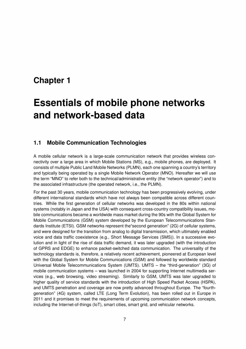
Figure 1.1: High-level view of a combined 2G/3G network.
The methodology proposed in this document is based on GSM and UMTS standards and networkarchitecture, although, with opportune modifications, it can be adapted to other mobile commu-nication standards, such as LTE. Hence, throughout the document, we will purposefully omittechnical details (e.g. additional components of the network architecture), under the assumptionthat the method developed here can also be adapted to 4G network architectures.
Hereafter we will use the term “2G” to refer to the ”GSM” access and “3G” for UMTS/HSPA access.Most operators maintain both a 2G and 3G network infrastructure, and therefore we will refer to asingle “2G/3G” infrastructure, like the one depicted in Fig. 1.1.
1.2 Mobile Network Architecture
The network architecture is composed of two main parts: the Radio Access Network (RAN) andthe Core Network (CN). The RAN includes all the “peripheral” components, i.e. the base stations1 that transmit / receive on the radio link from / to the MSs, and their respective controllers —called Base Station Controller (BSC) in GSM and Radio Network Controller (RNC) in UMTS. TheCN includes “back-end” equipments, whose physical location is normally concentrated at a fewsites.
It should be noted that there are actually two distinct CNs domains: the Circuit-Switched (CS),mainly for voice calls, and the Packet-Switched (PS) for data calls. The resulting high-level archi-tecture is sketched in Fig. 1.1. The network element that connect the CN to the RAN is the MobileSwitching Center (MSC) in the CS domain, and the SGSN in the PS domain. At any given time,a generic MS can be logically “attached” to the CS domain, to the PS domain, or both. Since ourprimary focus is on 2G/3G MSs that support voice services (as this are more likely associatedto persons, as discussed later in Section 1.6) hereafter we will restrict our attention to the CSdomain, unless differently specified2.
1The term “base station” is used hereafter to refer to jointly to the Base Transceiver Station (BTS) in GSM and tothe Node-B in UMTS.
2The distinction between CS and PS domains is slowly vanishing, with the progressive introduction of integratedMSC/SGSN equipments. However, for the purpose of this study it is useful to keep in mind the logical separation
8 of 64
CHAPTER 1. ESSENTIALS OF MOBILE PHONE NETWORKS AND NETWORK-BASED DATA
In modern networks, 2G and 3G systems coexist over the same infrastructure, as they operateon different portions of the frequency spectrum, i.e., different bands. Every MNO is assigneda different sub-band (or set thereof) for each system. Therefore, a generic point in space isgenerally serviced by different radio access technologies (2G and 3G) and by multiple MNOs.However, each MS can be “attached” only to one MNO and one access technology at any giventime3.
1.3 Cells
We now introduce the notion of “radio cell”, or simply “cell”. In cellular networks, geographicalradio coverage is provided by a multitude of base stations distributed across the serviced area.Each base station services one “cell”4. Each base station services a limited portion of space,called “cell coverage area”, or simply a “cell”. In turn, only MS terminals within a cell can connectto the associated base station.
The transmissions from each base station are optimised according to a set of modulation param-eters (e.g., carrier frequency in 2G, spreading code in 3G, antenna settings, transmit power) thatultimately affect the shape of the cell. Also, in order to avoid interference, each cell operates on apreassigned frequency band, which is different from that of the adjacent cells. Such a frequencyband allocation pattern, which is regularly repeated all over the network, can be described as achromatic range. Therefore, adjacent cells within a cluster can be denoted with different“colours”,indicating the operating frequency band. Finally, every point in space may be “covered” by multiplecells of different colours.
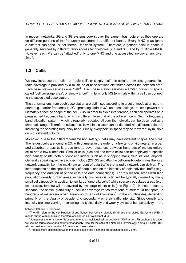
Moreover, due to the different transmission settings, cells may have different shapes and sizes.The largest cells are found in 2G, with diameter in the order of a few tens of kilometers. In urbanand suburban areas, cells areas tend to cover distances between hundreds of meters (micro-cells) and a few kilometers. Smaller cells (pico-cell and femto-cells) can be deployed at specifichigh-density points, both outdoor and indoor, such as in shopping malls, train stations, airports.Generally speaking, within each technology (2G, 3G and 4G) the cell density determines the localnetwork capacity, i.e., the maximum amount of data traffic that a radio network can deliver. Thelatter depends on the spatial density of people, and on the intensity of their individual traffic (e.g.,frequency and duration of phone calls and data connections). For this reason, areas with highpopulation density (urban areas, especially business districts) will be typically covered by manysmall cells (possibly in addition to few large “umbrella cells”) while sparsely populated areas (e.g.,countryside, forests) will be covered by few large macro-cells (see Fig. 1.2). Hence, in such ascenario, the spatial granularity of cellular coverage varies from tens of meters (in hot-spots) tohundreds of meters (in urban areas) up to tens of kilometers5 (in the countryside), dependingprimarily on the density of people, and secondarily on their traffic intensity. Since density andintensity are time-varying — following the typical daily and weekly cycles of human activity — the
between CS and PS domains.3The MS refers to the combination of one Subscriber Identity Module (SIM) and one Mobile Equipment (ME). A
mobile phone with dual-sim is therefore considered as two distinct MSs.4Sometimes the term “sector” is used to refer to an individual cell, especially in GSM jargon. Throughout this paper,
we use the terms sector and cell interchangeably. Also, for the sake of a simplified terminology, a single 3-sector BTSwill be considered as a bundle of 3 co-located base stations.
5The maximum distance between the base station and a generic MS attached to it is 35 km.
9 of 64
CHAPTER 1. ESSENTIALS OF MOBILE PHONE NETWORKS AND NETWORK-BASED DATA
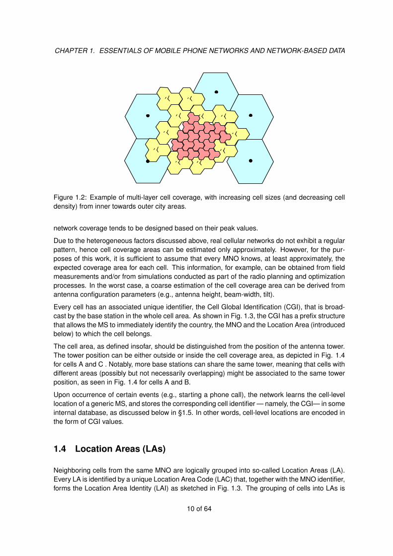
Figure 1.2: Example of multi-layer cell coverage, with increasing cell sizes (and decreasing celldensity) from inner towards outer city areas.
network coverage tends to be designed based on their peak values.
Due to the heterogeneous factors discussed above, real cellular networks do not exhibit a regularpattern, hence cell coverage areas can be estimated only approximately. However, for the pur-poses of this work, it is sufficient to assume that every MNO knows, at least approximately, theexpected coverage area for each cell. This information, for example, can be obtained from fieldmeasurements and/or from simulations conducted as part of the radio planning and optimizationprocesses. In the worst case, a coarse estimation of the cell coverage area can be derived fromantenna configuration parameters (e.g., antenna height, beam-width, tilt).
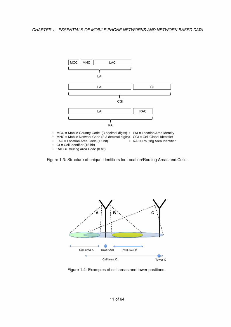
Every cell has an associated unique identifier, the Cell Global Identification (CGI), that is broad-cast by the base station in the whole cell area. As shown in Fig. 1.3, the CGI has a prefix structurethat allows the MS to immediately identify the country, the MNO and the Location Area (introducedbelow) to which the cell belongs.
The cell area, as defined insofar, should be distinguished from the position of the antenna tower.The tower position can be either outside or inside the cell coverage area, as depicted in Fig. 1.4for cells A and C . Notably, more base stations can share the same tower, meaning that cells withdifferent areas (possibly but not necessarily overlapping) might be associated to the same towerposition, as seen in Fig. 1.4 for cells A and B.
Upon occurrence of certain events (e.g., starting a phone call), the network learns the cell-levellocation of a generic MS, and stores the corresponding cell identifier — namely, the CGI— in someinternal database, as discussed below in §1.5. In other words, cell-level locations are encoded inthe form of CGI values.
1.4 Location Areas (LAs)
Neighboring cells from the same MNO are logically grouped into so-called Location Areas (LA).Every LA is identified by a unique Location Area Code (LAC) that, together with the MNO identifier,forms the Location Area Identity (LAI) as sketched in Fig. 1.3. The grouping of cells into LAs is
10 of 64
CHAPTER 1. ESSENTIALS OF MOBILE PHONE NETWORKS AND NETWORK-BASED DATA
MCC
• MCC = Mobile Country Code (3 decimal digits) • MNC = Mobile Network Code (2-3 decimal digits) • LAC = Location Area Code (16 bit) • CI = Cell Identifier (16 bit) • RAC = Routing Area Code (8 bit)
LAC
LAI
LAI
MNC
CI
CGI
• LAI = Location Area Identity • CGI = Cell Global Identifier • RAI = Routing Area Identifier
LAI RAC
RAI
Figure 1.3: Structure of unique identifiers for Location/Routing Areas and Cells.
Cell area A Tower A/B
Cell area C Tower C
Cell area B
A B C
Figure 1.4: Examples of cell areas and tower positions.
11 of 64
CHAPTER 1. ESSENTIALS OF MOBILE PHONE NETWORKS AND NETWORK-BASED DATA
Location Area 1
Routing Area 1-1
Routing Area 1-2
Routing Area 1-4
Routing Area 1-3
Cell 1-1-1 Cell 1-1-2
Cell 1-1-8
…
Cell 1-4-1 Cell 1-4-2
Cell 1-4-8
…
Location Area 2
Routing Area 2-1
Routing Area 2-2
Routing Area 2-4
Routing Area 2-3
Cell 2-1-1 Cell 2-1-2
Cell 2-1-8
…
Cell 2-4-1 Cell 2-4-2
Cell 2-4-8
…
MS i
Cell 1-4-2
RA 1-4
LA 1
MS i
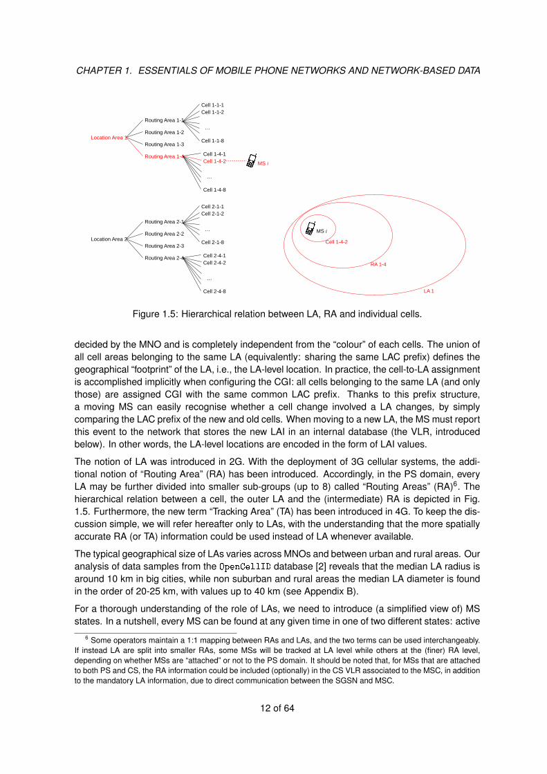
Figure 1.5: Hierarchical relation between LA, RA and individual cells.
decided by the MNO and is completely independent from the “colour” of each cells. The union ofall cell areas belonging to the same LA (equivalently: sharing the same LAC prefix) defines thegeographical “footprint” of the LA, i.e., the LA-level location. In practice, the cell-to-LA assignmentis accomplished implicitly when configuring the CGI: all cells belonging to the same LA (and onlythose) are assigned CGI with the same common LAC prefix. Thanks to this prefix structure,a moving MS can easily recognise whether a cell change involved a LA changes, by simplycomparing the LAC prefix of the new and old cells. When moving to a new LA, the MS must reportthis event to the network that stores the new LAI in an internal database (the VLR, introducedbelow). In other words, the LA-level locations are encoded in the form of LAI values.
The notion of LA was introduced in 2G. With the deployment of 3G cellular systems, the addi-tional notion of “Routing Area” (RA) has been introduced. Accordingly, in the PS domain, everyLA may be further divided into smaller sub-groups (up to 8) called “Routing Areas” (RA)6. Thehierarchical relation between a cell, the outer LA and the (intermediate) RA is depicted in Fig.1.5. Furthermore, the new term “Tracking Area” (TA) has been introduced in 4G. To keep the dis-cussion simple, we will refer hereafter only to LAs, with the understanding that the more spatiallyaccurate RA (or TA) information could be used instead of LA whenever available.
The typical geographical size of LAs varies across MNOs and between urban and rural areas. Ouranalysis of data samples from the OpenCellID database [2] reveals that the median LA radius isaround 10 km in big cities, while non suburban and rural areas the median LA diameter is foundin the order of 20-25 km, with values up to 40 km (see Appendix B).
For a thorough understanding of the role of LAs, we need to introduce (a simplified view of) MSstates. In a nutshell, every MS can be found at any given time in one of two different states: active
6 Some operators maintain a 1:1 mapping between RAs and LAs, and the two terms can be used interchangeably.If instead LA are split into smaller RAs, some MSs will be tracked at LA level while others at the (finer) RA level,depending on whether MSs are “attached” or not to the PS domain. It should be noted that, for MSs that are attachedto both PS and CS, the RA information could be included (optionally) in the CS VLR associated to the MSC, in additionto the mandatory LA information, due to direct communication between the SGSN and MSC.
12 of 64

CHAPTER 1. ESSENTIALS OF MOBILE PHONE NETWORKS AND NETWORK-BASED DATA
or idle. The MS spend most of its time in the “idle” state. It switch to “active” during voice callsand when engaged in the exchange of data packets with the network7. It switches to active statealso when exchanging signalling messages, without any trigger by the data or voice applications.It is important to remark that, at any given time, only a small minority of all MSs are found in activestate, the vast majority being in “idle” mode [13].
There are fundamental differences in the “behaviour” of MS during idle and active states, thattranslate into different levels of temporal and spatial accuracy when it comes to estimate theirlocation from network-side data, as explained below.
• MS in idle state. The MS is logically “attached” to one network8 but is not assigned anyradio resource. The MS “listens” (the broadcast channel of) one cell, but does not transmit.In idle states, decisions are taken autonomously by the MT: which cell to listen, and whetherand when to “jump” towards another cell (cell change), is determined autonomously by theMS internal logic, not by the network. The MS decision logic depends on the device vendorand is takes into account local measurements as well as past history.
By definition, MS in idle mode are passive receivers (i.e., they are not transmitting) thereforethe network has no way of detecting a cell change unless the MS decides to report this eventexplicitly. The MS reports the cell change only when it enters a new LAs, while cell changesinside the same LAs are not reported. In this way, the network can track the position of idleMSs only at the LA level, not at the cell level.
• MS in active state. The MS is assigned radio resources and is engaged in traffic exchange(voice, data or signalling) to and from the network. In active state, all decisions involvingradio resources are taken by network: this includes the determination of channel and cell,as well as whether and when to “jump” (handover) to another channel or cell. In this way,the network tracks the position of active MSs at the cell level.
From the above discussion, it should be clear that the network can “observe” the cell-level locationof each MS only at some specific times, and with a finite spatial resolution. In other words, giventhe “real” trajectory of a generic MS, continuous in time and space, the cellular network acts likea sensor that applies some form of sampling in time and quantisation in space.
1.5 Network-side data
There are several elements and subsystems within the network that maintain information aboutthe MS. Hereafter, we will discuss the ones more relevant for our study.
7Having a “data connection” (i.e., a PDP-context in 3G terminology) open does not imply that the MS is in “active”state. In fact, the MS can maintain the connection (logically) open for a long time without (physical) sending or receivingdata packets, in which case it would be persist in idle state. Generally speaking, the transition from “active” to “idle” istriggered by a short timeout (typically between 2 and 5 seconds) that is reset upon transmission or reception of newdata packets).
8Preferably their home MNO, if available, otherwise it will be “roaming” to another MNO
13 of 64

CHAPTER 1. ESSENTIALS OF MOBILE PHONE NETWORKS AND NETWORK-BASED DATA
1.5.1 Billing data: Call Detail Records (CDR)
For each voice and data connection (or part of it) the network elements generate “tickets” thatare sent to the billing system for charging purposes. The billing system stores these data in largedatabases, normally in the MNO warehouse. The term “Call Detail Records”, and especially itsacronym “CDR”9, is commonly used nowadays to indicate generically all billing records, includingthose originated from data connections.
The format of CDR is not standardised [3, 15] and there is a great deal of variability acrossdifferent implementations regarding the type of data contained in every CDR, as well as otherdetails of the CDR generation process (e.g., whether long calls are chunked into multiple CDRs).It is safe to assume that mobile CDR data contain at least the following information:
• International Mobile Subscriber Identifier (IMSI) (possibly encrypted).
• Starting time and duration of the call or connection.
• Type of call or connection (e.g. voice, SMS, data).
• Cell Global Identifier (CGI) of the starting cell, where the call or connection was initiated10.
Additional data might be optionally available for specific CDR implementations. For example, incase of handovers, CDR might include the identifiers of the subsequent visited cells, after thestarting cell. This is particularly relevant for long-lasting connections (e.g. always-on data con-nections for mobile phones). Other additional data include the IMEI, APN (for data connections)etc.
Historically, the CDR data were the first data source used in mobile phone data research, and stillthe overwhelming majority of studies and research project rely exclusively on CDR (see e.g. therecent survey [14].) This is mainly due to the fact that extracting CDR data for off-line processingis technically simple, given the non-volatile nature of such data, as discussed below.
1.5.2 Visitor Location Register (VLR)
The Visitor Location Register (VLR) and the Home Location Register (HLR) are database for sub-scriber data. The HLR stores the “permanent” subscriber parameter that are logically associatedto the Subscriber Identity Module (SIM), like e.g. the IMSI. The HLR is a central module servingthe whole MNO network, but is not very relevant for this study.
Basic VLR data
Logically speaking, each Mobile Switching Center (MSC) has its own associated VLR. The VLRcontains the “temporary” subscriber data for the MS currently “visiting” this MSC area. The mostrelevant VLR data for this study are the following mandatory fields:
9The terms “Call Data Records” and “Charging Data Records” are occasionally found in the literature in associationto their common acronym “CDR”.
10Strictly speaking, this is not a mandatory field [3] but we expect that most if not all MNOs actually include thisinformation in their CDR.
14 of 64
CHAPTER 1. ESSENTIALS OF MOBILE PHONE NETWORKS AND NETWORK-BASED DATA
• Location Area Identity (LAI)
• Temporary IMSI (T-IMSI).
These data, and especially the LAI, are used by the basic VLR-based method described later in§3.3.2. In addition to the mandatory fields above, some proprietary VLR implementations supportthe option of storing additional details, e.g., the time and CGI of the last message received by theMS. In case that such optional data are available, they can be used to considerably improve thespatial accuracy of the VLR method, as discussed later in §3.3.5.
Besides the MSCs, every Serving GPRS Support Node (SGSN) has also an associated VLR.The main difference between the VLR of circuit switching (CS) domain (traditionally associatedto voice traffic, at the mobile switching center (MSC)) and those of the packed switching (PS)domain (associated to data traffic at SGSN) is that the latter contain the Routing Area Identity(RAI) field instead of the LAI. A generic MS that is attached to both the CS and PS domains willlogically appear in two VLR, one for CS and one for PS. However, the distinction between CS VLRand PS VLR might not be important in practice, since the MSC and its neighbouring SGSN mightshare a single combined VLR — especially if the MSC and SGSN are themselves combined in asingle physical equipment. However, since our focus is on voice-enabled MSs, hereafter we willrefer exclusively to the VLR serving the CS domain — or both CS and PS, in case of combinedVLR.
The set of all VLR pertaining to all MSC in the MNO network collectively form a distributeddatabase. Therefore, hereafter we will use the singular term “VLR” to refer to the entire set ofVLR data across all MSCs.
Augmented VLR data
The standard Mobility Management procedures for 2G and 3G systems foresee the involvementof the MSC and/or SGSN whenever the MS engages in a new data connection, voice call orSMS and in general whenever the MS interacts with the network. During the message exchangebetween the MS and the MSC/SGSN the latter learns the current MS cell location. Although itis not mandatory for the VLR to record the cell nor the timestamp associated to such messageexchange, it is reasonable to expect that certain MNOs might decide to configure their VLR toretain these (optional) data in addition to the mandatory LAI/T-IMSI fields11.
In this case, the VLR data is enriched with the identifier of the last “observed” cell within thecurrent LA along with the associated timestamp, for every generic MS. Such “augmented” VLRwould therefore merge together the two types of data that we have previously encountered, sep-arately, in the basic VLR-only and CDR-only methods: cell-level and LA-level locations. Further-more, augmented VLR data could provide cell-level location also for MS that did not engage inSMS/voice/data connections, provided that they performed some kind of signalling procedure,e.g. Location Area Update (LAU). In other words, they bear the potential to “observe” the cell-level location of a larger fraction of MS than what is possible with CDR data. The estimationmethod described later in Chapter 3 is designed to cope with the data heterogeneity derivingfrom a combination of cell-level and LA-level records.
11In fact, the marginal cost of storing this information in the VLR is in general small, and augmented VLR data canbe exploited to implement supplementary (non standard) functions and/or certain forms of MNO-specific optimisations.
15 of 64

CHAPTER 1. ESSENTIALS OF MOBILE PHONE NETWORKS AND NETWORK-BASED DATA
Phone call in cell C.2
time
space
t4 t1
cells
A.4
A.3
A.2
A.1
B.3
B.2
B.1
C.3
C.2
C.1
LA
A
B
C
t2 t3
Enter LA A
SMS in cell A.3
Enter LA B
(a) Ground truth
time
space
t* t4 t1
cells
A.4
A.3
A.2
A.1
B.3
B.2
B.1
C.3
C.2
C.1
LA
A
B
C
t2 t3
A.3
C.2
(b) CDR
time
space
t* t4 t1
cells
A.4
A.3
A.2
A.1
B.3
B.2
B.1
C.3
C.2
C.1
LA
A
B
C
t2 t3
LA C
LA B
LA A
(c) VLR
time
space
t* t4 t1
cells
A.4
A.3
A.2
A.1
B.3
B.2
B.1
C.3
C.2
C.1
LA
A
B
C
t2 t3
A.3
C.2
LA C
LA B
LA A
(d) Joint CDR and VLR
time
space
t* t4 t1
cells
A.4
A.3
A.2
A.1
B.3
B.2
B.1
C.3
C.2
C.1
LA
A
B
C
t2 t3
A.3
A.1
B.1
C.2
LA C
LA B
LA A
(e) Augmented VLR
Figure 1.6: Schematic representation of observed trajectory for different network-based data.
16 of 64
CHAPTER 1. ESSENTIALS OF MOBILE PHONE NETWORKS AND NETWORK-BASED DATA
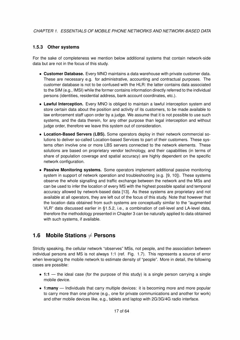
1.5.3 Other systems
For the sake of completeness we mention below additional systems that contain network-sidedata but are not in the focus of this study.
• Customer Database. Every MNO maintains a data warehouse with private customer data.These are necessary e.g. for administrative, accounting and contractual purposes. Thecustomer database is not to be confused with the HLR: the latter contains data associatedto the SIM (e.g., IMSI) while the former contains information directly referred to the individualpersons (identities, residential address, bank account coordinates, etc.).
• Lawful Interception. Every MNO is obliged to maintain a lawful interception system andstore certain data about the position and activity of its customers, to be made available tolaw enforcement staff upon order by a judge. We assume that it is not possible to use suchsystems, and the data therein, for any other purpose than legal interception and withoutjudge order, therefore we leave this system out of consideration.
• Location-Based Servers (LBS). Some operators deploy in their network commercial so-lutions to deliver so-called Location-based Services to part of their customers. These sys-tems often involve one or more LBS servers connected to the network elements. Thesesolutions are based on proprietary vendor technology, and their capabilities (in terms ofshare of population coverage and spatial accuracy) are highly dependent on the specificnetwork configuration.
• Passive Monitoring systems. Some operators implement additional passive monitoringsystem in support of network operation and troubleshooting (e.g. [9, 10]). These systemsobserve the whole signalling and traffic exchange between the network and the MSs andcan be used to infer the location of every MS with the highest possible spatial and temporalaccuracy allowed by network-based data [13]. As these systems are proprietary and notavailable at all operators, they are left out of the focus of this study. Note that however thatthe location data obtained from such systems are conceptually similar to the “augmentedVLR” data discussed earlier in §1.5.2, i.e., a combination of cell-level and LA-level data,therefore the methodology presented in Chapter 3 can be naturally applied to data obtainedwith such systems, if available.
1.6 Mobile Stations 6= Persons
Strictly speaking, the cellular network “observes” MSs, not people, and the association betweenindividual persons and MS is not always 1:1 (ref. Fig. 1.7). This represents a source of errorwhen leveraging the mobile network to estimate density of “people”. More in detail, the followingcases are possible:
• 1:1 — the ideal case (for the purpose of this study) is a single person carrying a singlemobile device.
• 1:many — Individuals that carry multiple devices: it is becoming more and more popularto carry more than one phone (e.g., one for private communications and another for work)and other mobile devices like, e.g., tablets and laptop with 2G/3G/4G radio interface.
17 of 64

CHAPTER 1. ESSENTIALS OF MOBILE PHONE NETWORKS AND NETWORK-BASED DATA
• 1:0 — some persons do not carry any mobile phone.
• 0:1 — MS that are not associated to any person: these MS are associated to “things”, notindividual persons, and use the mobile network for machine-to-machine (M2M) communi-cations.
The 1:many and 0:1 cases introduce positive errors (overcounting), while 1:0 introduces negativeerror (undercounting). We expect that the frequency of 1:many and 1:0 cases varies across de-mographic groups, i.e., that correlations exist between the number of personal devices and certaindemographic attributes (age and profession above all). For this reason, 1:0 and 1:many casesare likely to introduce a bias, with certain age/professional groups under- or over-represented.
In order to mitigate (yet, not completely eliminate) the over-counting errors “0:1” and “1:many”, apossible approach is to restrict the analysis to data from the CS domain. This will automaticallyexclude those data-only devices that are designed to attach only to the PS domain. For VLR data,this implies restricting to MSC data, and to exclude SGSN data.
Besides this initial filtering, it is possible to further mitigate the over-counting error by adoptingmore sophisticated (i.e., implicit or explicit) filtering strategies. For instance, one approach is toidentify and filter out MSs that are not enabled for voice calls. This can be done by accountingfor the Type Allocation Code (TAC) code included in the International Mobile Station EquipmentIdentity (IMEI) – if available in the CDR/VLR, or by integration with other data sources– from theAPN, or heuristically by simply picking MS that never engaged in a voice call during a reasonablylong observation period (e.g. over 24 hours). All the above methods tend to rely on data fieldsthat are optional and/or additional data sources, and their cost of implementation and effective-ness are highly dependent on the particular network setting. In other words, it is not possibleto define a single mitigation approach that fits for all MNOs, but this heterogeneity should notdiscourage a MNO to put in place additional processing function, based on MNO-specific config-uration, aimed at removing or anyway reducing some of the known sources of error (e.g. filteringof M2M terminals).
Mobile Network Operator (MNO)
Mobile Terminal (MT)
Person
1:1
1:0
1:many
0:1
Figure 1.7: Possible association schemes between Mobile Stations and persons.
18 of 64
Chapter 2
Measuring population densitydistribution in support of public policy:requirements and definitions
2.1 Overview of the general approach
The vast literature on mobile phone data insofar is constituted by studies conducted for a specificpurpose on datasets from a single MNO (see [14] for a recent survey). In rare cases datasetsfrom different MNOs were compared (e.g. [8]). One distinctive goal of this study is to develop amethodology that allows data from different MNOs to be fused. The union of data from MNOsacross different countries would allow to produce a pan-European view of population density.Furthermore, the proper fusion of multi-MNO data from the same country bears the potentialof improving the accuracy of the estimation within the same country along different directions,namely: (i) increase the population coverage; (ii) mitigate the potential bias caused by MNO-specific network configurations and (iii) improve the spatial accuracy (this point is discussed laterat the end of §3.5).
In order to be applicable to multiple MNOs, the proposed methodology must rely on data that arecommonly available at every MNO — as needed for the operation of the network and associatedmobile services — and that can be extracted at reasonable cost. Moreover, particular attentionmust be paid to avoid jeopardisation of business confidentiality and user privacy.
We envision the data and computation flow depicted in Fig. 2.1, consisting of two stages. Thefirst stage algorithm, termed “local processing”, is run independently within each MNO: it takes ininput a set of “micro-data” and returns in output a set of highly aggregated intermediate data.
The input data are termed “micro” because every record (from CDR and/or VLR databases) isreferred to individual MS. The local processing module will take in input also network topologydata about position and coverage area (footprint) of every cell, and optionally additional datasources available within the MNO that might help to identify and filter out MS not associated tohuman users (e.g., M2M terminals).
It is important to remark that with the proposed method micro-data do not leave the MNO domain.For every MNO, the output of the local processing module is a set of vector data that collectively
19
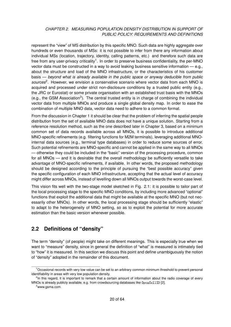
CHAPTER 2. MEASURING POPULATION DENSITY DISTRIBUTION IN SUPPORT OFPUBLIC POLICY: REQUIREMENTS AND DEFINITIONS
represent the “view” of MS distribution by this specific MNO. Such data are highly aggregate overhundreds or even thousands of MSs: it is not possible to infer from there any information aboutindividual MSs (location, trajectory, identity, calling patterns, etc.) and therefore such data arefree from any user-privacy criticality1. In order to preserve business confidentiality, the per-MNOvector data must be constructed in a way to avoid leaking business sensitive information — e.g.,about the structure and load of the MNO infrastructure, or the characteristics of his customerbasis — beyond what is already available in the public space or anyway deducible from publicsources2. However, we envision a conservative scenario where vector data from each MNO isacquired and processed under strict non-disclosure conditions by a trusted public entity (e.g.,the JRC or Eurostat) or some private organisation with an established trust basis with the MNOs(e.g., the GSM Association3). The central trusted entity is in charge of combining the individualvector data from multiple MNOs and produce a single global density map. In order to ease thecombination of multiple MNO data, vector data need to adhere to a common format.
From the discussion in Chapter 1 it should be clear that the problem of inferring the spatial peopledistribution from the set of available MNO data does not have a unique solution. Starting from areference resolution method, such as the one described later in Chapter 3, based on a minimumcommon set of data records available across all MNOs, it is possible to introduce additionalMNO-specific refinements (e.g. filtering functions for M2M terminals), leveraging additional MNO-internal data sources (e.g., terminal type databases) in order to reduce some sources of error.Such potential refinements are MNO-specific and cannot be applied in the same way to all MNOs— otherwise they could be included in the “basic” version of the processing procedure, commonfor all MNOs — and it is desirable that the overall methodology be sufficiently versatile to takeadvantage of MNO-specific refinements, if available. In other words, the proposed methodologyshould be designed according to the principle of pursuing the “best possible accuracy” giventhe specific configuration of each MNO infrastructure, accepting that the actual level of accuracymight differ across MNOs, instead of levelling down all MNOs output towards the worst-case level.
This vision fits well with the two-stage model sketched in Fig. 2.1: it is possible to tailor part ofthe local processing stage to the specific MNO conditions, by including more advanced “optional”functions that exploit the additional data that might be available at the specific MNO (but not nec-essarily other MNOs). In other words, the local processing stage should be sufficiently “elastic”to adapt to the heterogeneity of MNO setting, so as to exploit the potential for more accurateestimation than the basic version whenever possible.
2.2 Definitions of “density”
The term “density” (of people) might take on different meanings. This is especially true when wewant to “measure” density, since in general the definition of “what” is measured is intimately tiedto “how” it is measured. In this section we discuss this point and define unambiguously the notionof “density” adopted in the remainder of this document.
1Occasional records with very low value can be set to an arbitrary common minimum threshold to prevent personalidentifiability in areas with very low population density.
2In this regard, it is important to remark that a certain amount of information about the radio coverage of everyMNOs is already publicly available, e.g. from crowdsourcing databases like OpenCellID [2].
3www.gsma.com.
20 of 64
CHAPTER 2. MEASURING POPULATION DENSITY DISTRIBUTION IN SUPPORT OFPUBLIC POLICY: REQUIREMENTS AND DEFINITIONS
Local Processing
intermediate macrodata
m
MNO m
Local Processing
MNO m+1
Local Processing
Raw µdata
MNO m+2
Global Processing
Total Density Map
Trusted Organization (e.g., JRC, Eurostat)
intermediate macrodata
m+1
intermediate macrodata
m+2
Raw µdata
Raw µdata
Figure 2.1: General scheme of data and computation flow. Micro-data do not leave the respectiveMNO domains. Only (intermediate) macro-data are exported by MNOs to the central organisationfor multi-MNO data fusion.
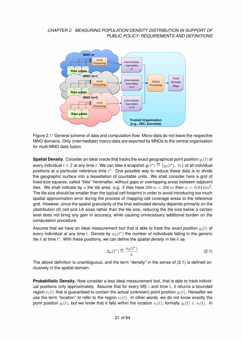
Spatial Density. Consider an ideal oracle that tracks the exact geographical point position yi(t) ofevery individual i ∈ I at any time t. We can take a snapshot y(t∗)
def
= yi(t∗), ∀i of all individualpositions at a particular reference time t∗. One possible way to reduce these data is to dividethe geographic surface into a tessellation of countable units. We shall consider here a grid offixed-size squares, called “tiles” hereinafter, without gaps or overlapping areas between adjacenttiles. We shall indicate by a the tile area: e.g. if tiles have 200m × 200m then a = 0.04 km2.The tile size should be smaller than the typical cell footprint in order to avoid introducing too muchspatial approximation error during the process of mapping cell coverage areas to the referencegrid. However, since the spatial granularity of the final estimated density depends primarily on the(distribution of) cell and LA sizes rather than the tile size, reducing the tile size below a certainlevel does not bring any gain in accuracy, while causing unnecessary additional burden on thecomputation procedure.
Assume that we have an ideal measurement tool that is able to track the exact position yi(t) ofevery individual at any time t. Denote by nk(t∗) the number of individuals falling in the generictile k at time t∗. With these positions, we can define the spatial density in tile k as
∆k(t∗)
def
=nk(t
∗)
a. (2.1)
The above definition is unambiguous, and the term “density” in the sense of (2.1) is defined ex-clusively in the spatial domain.
Probabilistic Density. Now consider a less ideal measurement tool, that is able to track individ-ual positions only approximately. Assume that for every MS i and time t, it returns a boundedregion νi(t) that is guaranteed to contain the actual (unknown) point position yi(t). Hereafter weuse the term “location” to refer to the region νi(t). In other words, we do not know exactly thepoint position yi(t), but we know that it falls within the location νi(t), formally yi(t) ∈ νi(t). In
21 of 64
CHAPTER 2. MEASURING POPULATION DENSITY DISTRIBUTION IN SUPPORT OFPUBLIC POLICY: REQUIREMENTS AND DEFINITIONS
practice, the location will represent (an approximation of) of the coverage area of a cell or LA,hereafter referred to as “cell-level locations” and “LA-level locations” respectively.
For the sake of simplicity, consider a quantised geographical space where every location νi(t)maps to a set of tiles on the regular reference grid. Let |νi(t)| denote the (integer) number oftiles enclosed by νi(t). Without any further information, we must assume that a MS i can befound equally likely at every point within νi(t). This means that the MS i is present (i-th uniformprobability 1
|νi(t)| ) in each tile within the associated location (and with zero probability outside).We now introduce the binary indicator function δk∈ui(t) to indicate whether the generic tile k isincluded in location νi(t), formally: δk∈νi(t) = 1 ⇔ k ∈ νi(t). From such data, we can still definethe “density” in the generic tile k as:
∆k(t∗)
def
=1
a·
I∑i=1
δk∈νi(t)
|νi(t∗)|(2.2)
wherein I denotes the total number of MS. Definition (2.2) has a different interpretation than (2.1)as it embeds a probabilistic dimension in addition to the spatial one. In fact, the value of ∆k(t
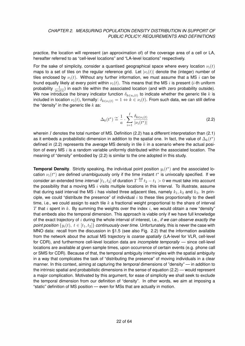
∗)defined in (2.2) represents the average MS density in tile k in a scenario where the actual posi-tion of every MS i is a random variable uniformly distributed within the associated location. Themeaning of “density” embodied by (2.2) is similar to the one adopted in this study.
Temporal Density. Strictly speaking, the individual point position yi(t∗) and the associated lo-cation νi(t∗) are defined unambiguously only if the time instant t∗ is univocally specified. If weconsider an extended time interval [t1, t2] of duration T def
= t2 − t1 > 0 we must take into accountthe possibility that a moving MS i visits multiple locations in this interval. To illustrate, assumethat during said interval the MS i has visited three adjacent tiles, namely k1, k2 and k3. In prin-ciple, we could “distribute the presence” of individual i to these tiles proportionally to the dwelltime, i.e., we could assign to each tile k a fractional weight proportional to the share of intervalT that i spent in k. By summing the weights over the index i, we would obtain a new “density”that embeds also the temporal dimension. This approach is viable only if we have full knowledgeof the exact trajectory of i during the whole interval of interest, i.e., if we can observe exactly thepoint position yi(t), t ∈ [t1, t2] continuously over time. Unfortunately, this is never the case withMNO data: recall from the discussion in §1.5 (see also Fig. 2.2) that the information availablefrom the network about the actual MS trajectory is coarse spatially (LA-level for VLR, cell-levelfor CDR), and furthermore cell-level location data are incomplete temporally — since cell-levellocations are available at given sample times, upon occurrence of certain events (e.g. phone callor SMS for CDR). Because of that, the temporal ambiguity intermingles with the spatial ambiguityin a way that complicates the task of “distributing the presence” of moving individuals in a clearmanner. In this context, aiming at capturing the temporal dimensions of ”density” — in addition tothe intrinsic spatial and probabilistic dimensions in the sense of equation (2.2) — would representa major complication. Motivated by this argument, for ease of simplicity we shall seek to excludethe temporal dimension from our definition of “density”. In other words, we aim at imposing a“static” definition of MS position — even for MSs that are actually in motion.
22 of 64

CHAPTER 2. MEASURING POPULATION DENSITY DISTRIBUTION IN SUPPORT OFPUBLIC POLICY: REQUIREMENTS AND DEFINITIONS
Space Coarser granularity
Finer granularity
Time
Continuous
Sampled cell-level data (CDR)
LA-level data (VLR)
(a)
Spatial resolution
high
Temporal resolution
high
low cell-level data
(CDR)
LA-level data (VLR)
low
(b)
Figure 2.2: High-level comparison between the spatial and temporal dimensions of cell-level andLA-level data respectively in CDR and VLR.
2.3 Dealing with MS movements
Assume we aim at measuring the population density at a reference time t∗. If we were able to“sample” the position of all MSs at the same reference time t∗, than we would simply ignorewhether each MS is moving or not at this time, and the problem of temporal ambiguity wouldsimply not arise. In our context, this is possible only with LA-level locations obtained from VLR:recall that the MS must communicate to the network every change of LA (via so-called LocationArea Update procedure), therefore the LA-level location is monitored continuously in time.
With cell-level locations instead (from CDR or augmented VLR), the number of MS that canbe “observed” at a generic time t∗ is only a small fraction of the whole MS population, alsoat peak hour. This is due to the fact that cell-level locations are revealed to the network onlyupon occurrence of specific events (starting a phone call or SMS, engaging in a data connection,initiating a signalling procedure etc.), therefore are observed only at specific “sampling times”.
The duality between cell-level and LA-level data in terms of temporal continuity and spatial gran-ularity is summarised in Fig. 2.2(a).
When cell-level locations are considered (e.g., from CDR) we need to consider records along aninterval of reasonably long duration, say one or a few hours, in order to “observe” (the cell-levellocations of) a sufficiently large number of MSs. But then the problem arises: which locationto pick as representative of the position of MS i during an interval of non-null duration? Wepropose to pick the observed location nearest in time to the reference time t∗, i.e., the cell locationwith the closest timestamp to t∗, subject to minimum and maximum temporal limits. Formally:consider a generic MS i that was observed at the set of locations νi(t1), νi(t2), ... respectivelyat the set of observation times T def
= t1, t2...; denote by t∗ 6∈ T the reference time and byW def
= [t∗− θl, t∗+ θu] an observation window of duration W = θl + θu around the reference time;we define the “proxy” location νi(t∗) of MS i at time t∗ as the location observed at the nearestobservation time t∗, i.e., νi(t∗)
def
= νi(t∗) with:
23 of 64
CHAPTER 2. MEASURING POPULATION DENSITY DISTRIBUTION IN SUPPORT OFPUBLIC POLICY: REQUIREMENTS AND DEFINITIONS
t∗def
= argmint∈T ∩W
|t− t∗| (2.3)
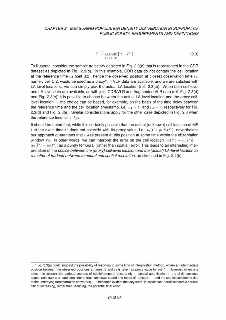
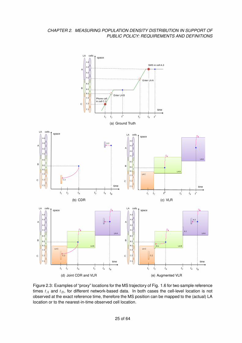
To illustrate, consider the sample trajectory depicted in Fig. 2.3(a) that is represented in the CDRdataset as depicted in Fig. 2.3(b). In this example, CDR data do not contain the cell locationat the reference time tA (cell B.2), hence the observed position at closest observation time t1,namely cell C.2, would be used as a proxy4. If VLR data are available, and we are satisfied withLA-level locations, we can simply pick the actual LA location (ref. 2.3(c)). When both cell-leveland LA-level data are available, as with joint CDR/VLR and Augmented VLR data (ref. Fig. 2.3(d)and Fig. 2.3(e)) it is possible to choose between the actual LA-level location and the proxy cell-level location — the choice can be based, for example, on the basis of the time delay betweenthe reference time and the cell location timestamp, i.e. tA − t1 and tA − t2 respectively for Fig.2.3(d) and Fig. 2.3(e). Similar considerations apply for the other case depicted in Fig. 2.3 whenthe reference time fall in tB .
It should be noted that, while it is certainly possible that the actual (unknown) cell location of MSi at the exact time t∗ does not coincide with its proxy value, i.e., νi(t∗) 6= νi(t
∗), neverthelessour approach guarantees that i was present at this position at some time within the observationwindow W . In other words, we can interpret the error on the cell location |νi(t∗) − νi(t
∗)| =|νi(t∗)− νi(t∗)| as a purely temporal (rather than spatial) error. This leads to an interesting inter-pretation of the choice between the (proxy) cell-level location and the (actual) LA-level location asa matter of tradeoff between temporal and spatial resolution, ad sketched in Fig. 2.2(b).
4Fig. 2.3(a) could suggest the possibility of resorting to some kind of interpolation method, where an intermediateposition between the observed positions at times t1 and t4 is taken as proxy value for νi(t∗). However, when onetakes into account the various sources of spatio/temporal uncertainty — spatial quantisation in the bi-dimensionalspace; unknown start and stop time of trips; unknown speed and mode of transport — and the spatial constraints dueto the underlying transportation network(s) — it becomes evident that any such “interpolation” heuristic bears a seriousrisk of increasing, rather than reducing, the potential final error.
24 of 64
CHAPTER 2. MEASURING POPULATION DENSITY DISTRIBUTION IN SUPPORT OFPUBLIC POLICY: REQUIREMENTS AND DEFINITIONS
Phone call in cell C.2
time
space
t4 t1
cells
A.4
A.3
A.2
A.1
B.3
B.2
B.1
C.3
C.2
C.1
LA
A
B
C
t2 t3
Enter LA A
SMS in cell A.3
Enter LA B
t* t*
(a) Ground Truth
time
space
tA t4
t1
cells
A.4
A.3
A.2
A.1
B.3
B.2
B.1
C.3
C.2
C.1
LA
A
B
C
t2 t3
C.2
tB
A.3
(b) CDR
time
space
t* t4 t1
cells
A.4
A.3
A.2
A.1
B.3
B.2
B.1
C.3
C.2
C.1
LA
A
B
C
t2 t3
LA C
LA B
LA A
t* t*
(c) VLR
time
space
tA t4
t1
cells
A.4
A.3
A.2
A.1
B.3
B.2
B.1
C.3
C.2
C.1
LA
A
B
C
t2 t3
C.2
LA C
LA B
LA A
tB
(d) Joint CDR and VLR
time
space
tA t4
t1
cells
A.4
A.3
A.2
A.1
B.3
B.2
B.1
C.3
C.2
C.1
LA
A
B
C
t2 t3
A.3
A.1
B.1
C.2
LA C
LA B
LA A
tB
(e) Augmented VLR
Figure 2.3: Examples of “proxy” locations for the MS trajectory of Fig. 1.6 for two sample referencetimes tA and tB , for different network-based data. In both cases the cell-level location is notobserved at the exact reference time, therefore the MS position can be mapped to the (actual) LAlocation or to the nearest-in-time observed cell location.
25 of 64

Chapter 3
Measurement Methodology
In this Chapter we describe the proposed methodological framework for the task of estimatingpopulation density from multi-MNO data. We aim at providing a framework that is general enoughto be implemented by any European MNOs — hence, does not rely on MNO-specific aspectslike network configuration, data organisation etc. — but at the same time is flexible enough totake advantage (optionally) from potential MNO-specific improvements (e.g., availability of moreaccurate location data).
The proposed methodology can be applied to one-time analyses as well as to the periodical (of-fline) analyses, e.g., based on daily or monthly activity. In addition, the proposed approach issuitable to continuous online analyses, although such an option requires considerably more en-gineering efforts, especially at network modeling level, in order to ensure consistency of networktopology data accounting for changes and upgrades. As the engineering aspects remain outsidethe scope of this study, hereafter we assume a static (known) network topology.
3.1 Overview of the measurement methodology
The proposed methodology relies on two distinct types of data:
• Network Topology data about the geographical location and coverage areas of radio cells.
• MS Counters of the number of MS observed (at the reference time) on every cell and LAs.
Two main contributions of this work are:
• We consider extended topology data and assume (approximate) knowledge of the wholecell coverage area, instead of merely the (exact) tower location.
• Our method can combine MS counters at different spatial granularity, i.e., at cell-level andLA-level, obtained from CDR and/or VLR databases, rather than exclusively cell-level datafrom CDR.
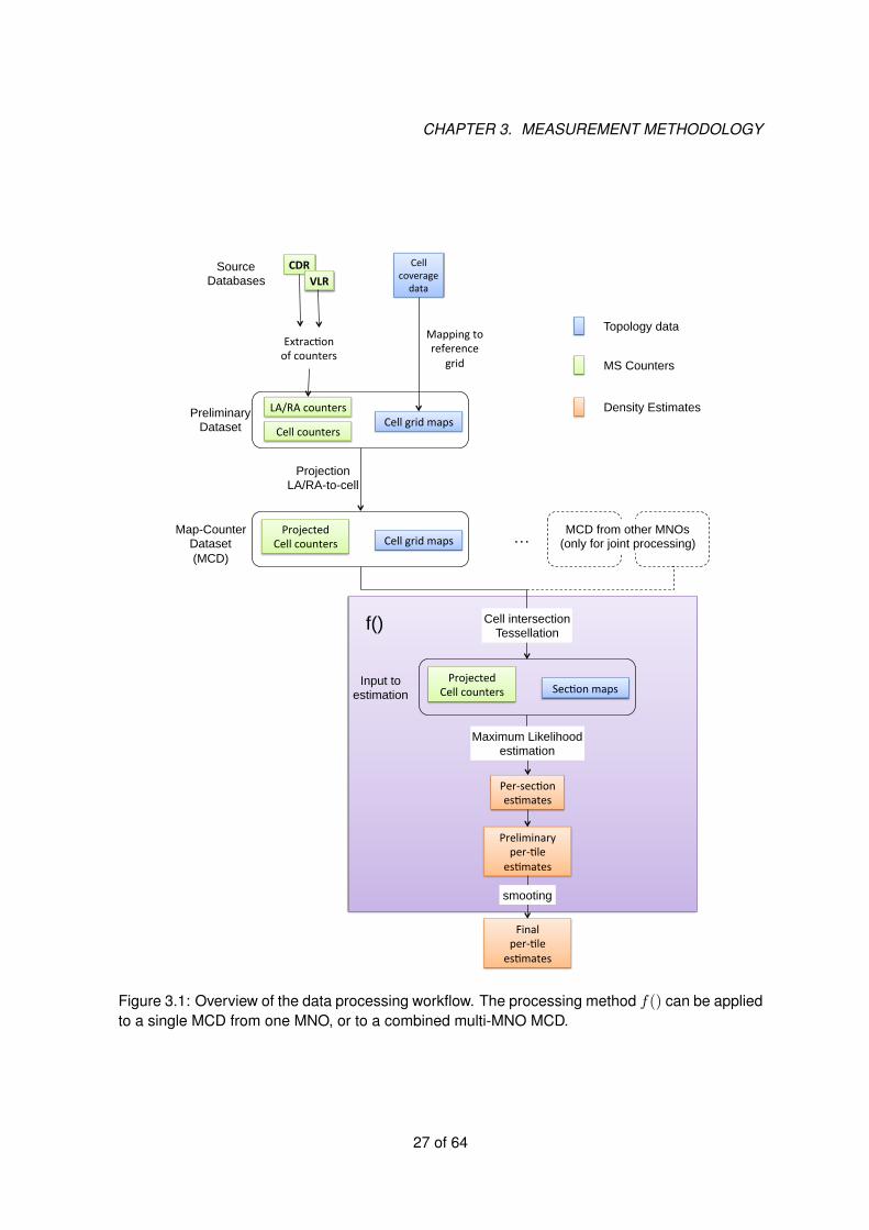
The proposed measurement method can be described as a chain of intermediate data processingstages. A high-level view of the data workflow is sketched in Fig. 3.1. Each processing stage isdetailed in the following sections of this chapter.
26
CHAPTER 3. MEASUREMENT METHODOLOGY
Extrac'on of counters
Projection LA/RA-to-cell
Preliminary Dataset
CDR Cell coverage data VLR
LA/RA counters
Cell counters Cell grid maps
Projected Cell counters
Per-‐sec'on es'mates
Preliminary per-‐'le es'mates
Source Databases
Mapping to reference
grid
Cell grid maps Map-Counter
Dataset (MCD)
Projected Cell counters Sec'on maps
Input to estimation
Cell intersection Tessellation
Final per-‐'le es'mates
Maximum Likelihood estimation
smooting
Topology data
MS Counters
Density Estimates
… MCD from other MNOs (only for joint processing)
f()
Figure 3.1: Overview of the data processing workflow. The processing method f() can be appliedto a single MCD from one MNO, or to a combined multi-MNO MCD.
27 of 64

CHAPTER 3. MEASUREMENT METHODOLOGY
The network topology data (i.e., cell maps) for each MNO are mapped to a common reference gridin order to facilitate the fusion of data from different MNO. We recommend to adopt the INSPIREreference grid specified in [12] for this purpose. In fact, the INSPIRE specification provides acommon framework for harmonized and interoperable geographic localization of different typesof spatial objects and quantities, and it is specifically intended for statistical reporting purposes. Itappears to be perfectly suited for the purpose of fusing aggregated data from different EuropeanMNOs. Furthermore, it greatly facilitates the prospective integration of multi-MNO data with othersources of spatial data and services. Hereafter we will adopt the term “tile" to refer to a genericspatial unit in the reference grid1.
At some point during the workflow, the generic MNO m generates a set of “map-counter" records(bj , cj), each record referring to a different radio cell j in its network. In a nutshell, bj denotesthe map of cell j on the reference grid, while cj denotes the number of MS “observed" in cell jaccording to the available CDR/VLR data — both elements are formally introduced in Fig. 3.5.The whole set of map-counter records from a generic MNO m constitutes the the “Map-CounterDataset" (MCD for short) and will be denoted by Sm (ref. Fig. 3.2(a)). MCD is an importantintermediate data along the data processing flow.
We can envision two possible options with respect to the subsequent processing of MCD datafrom different MNOs. In the first option, depicted in Fig. 3.2(c), all MNOs would agree to pass theirMCD datasets to a central trusted entity (e.g., Eurostat or JRC). The latter would then estimatethe total density map DT by jointly processing the union of individual MCDs from all MNOs, i.e.:
DJ = f (S1,S2, . . .) = f
(⋃m
Sm
)(3.1)
where f() denotes the data processing method that is detailed later through sections §3.5-§3.7.
The advantage of this option is that the final density estimation can leverage in the best possibleway data diversity — in terms of spatial coverage and population coverage — across differentMNOs. Note that no privacy-critical information would be disclosed in this way, since map-counterrecords are aggregate data, not micro-data. However, this approach requires every MNOs toexport information that might be regarded as critical from a business perspective (e.g., detailedsize, location and traffic load of individual cells). Although the recipient of such data would beanyway a trusted entity, bound to non-disclosure legal constraints, it is not clear whether suchmodel would be accepted by MNOs.
This motivates the definition of an alternative, more conservative scenario, where the MCD pro-cessing is split into two stages as sketched in Fig. 3.2(b) (see also Fig. 2.1). In the first stage,each MNO computes a “partial" density map Dm from its local MCD data, independently fromother MNOs. In the second stage, the central entity simply combines the density maps from differ-ent MNOs into the final “global" density map DΣ. In other words, the function f() of equation (3.1)is run by every MNO based exclusively on local data, and the (local) outputs are then exported tothe central entity for final (weighted) summation, formally:
Dm = f (Sm) , ∀m. (3.2)
DΣ =∑m
wmDm (3.3)
1Note that in [12] the term “cell" is used to refer to the spatial grid units. In the context of the present work, thiscollides with the usage of the term “cell" to denote radio coverage areas for the mobile network.
28 of 64

CHAPTER 3. MEASUREMENT METHODOLOGY
b1 =
b2 =
bj =
c1= 153
c2= 345
cj= 246
…
map-counter record for cell j
Map/Counter Dataset (MCD)
for MNO m Sm
…
(a) MCD dataset from individual MNO…
MCD Sm from MNO m
…
Joint Density Map DJ
MCD Sm+1 from MNO m+1
MCD Sm+2 from MNO m+2
Trusted Organization (e.g., JRC, Eurostat)
f()
(b) Joint MCD processing from multiple MNOs
…
MCD Sm from MNO m
…
f()
f()
f()
Σ
Density map Dm+1
Density map Dm+2
Global Density Map DG
Density map Dm
MCD Sm+1 from MNO m+1
MCD Sm+2 from MNO m+2
Trusted Organization (e.g., JRC, Eurostat)
(c) Local MCD processing within each MNO
Figure 3.2: Schematic representation of multi-MNO data processing. The function f() denotesthe data processing method detailed through sections §3.5-§3.7. It can be applied for the jointprocessing of all MCDs (b) as well as for the separate processing of each individual MCD (c).
29 of 64
CHAPTER 3. MEASUREMENT METHODOLOGY
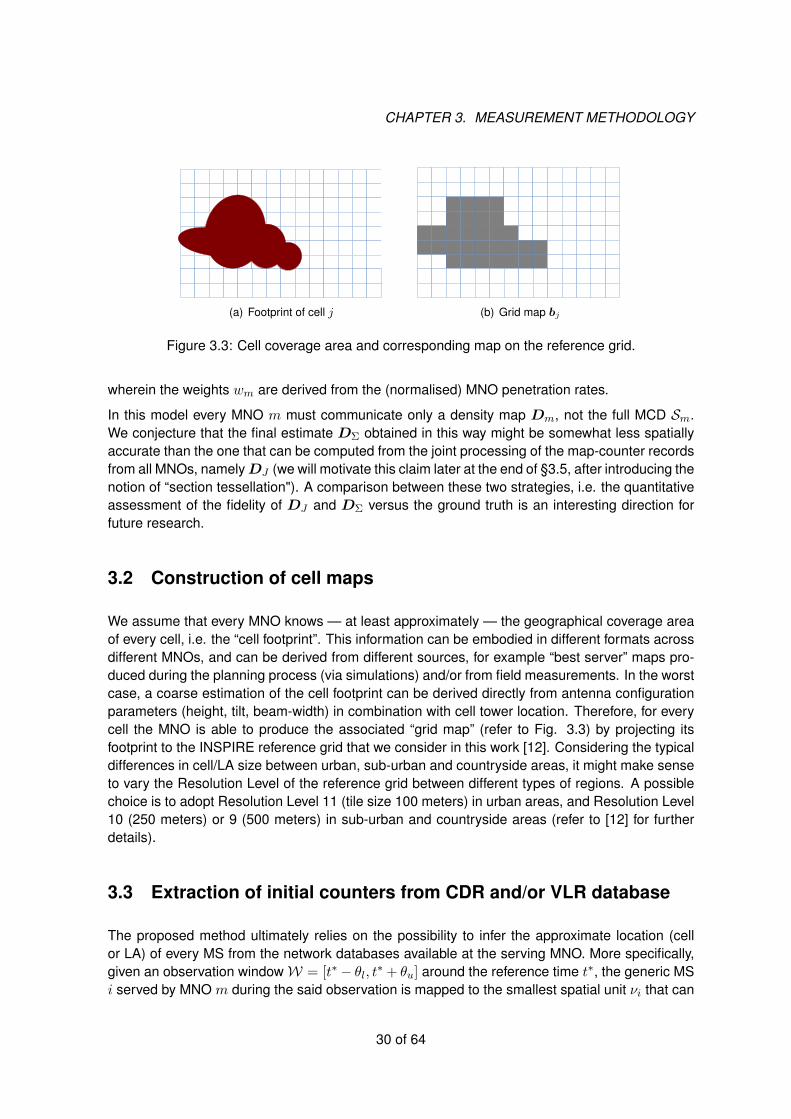
(a) Footprint of cell j (b) Grid map bj
Figure 3.3: Cell coverage area and corresponding map on the reference grid.
wherein the weights wm are derived from the (normalised) MNO penetration rates.
In this model every MNO m must communicate only a density map Dm, not the full MCD Sm.We conjecture that the final estimate DΣ obtained in this way might be somewhat less spatiallyaccurate than the one that can be computed from the joint processing of the map-counter recordsfrom all MNOs, namely DJ (we will motivate this claim later at the end of §3.5, after introducing thenotion of “section tessellation"). A comparison between these two strategies, i.e. the quantitativeassessment of the fidelity of DJ and DΣ versus the ground truth is an interesting direction forfuture research.
3.2 Construction of cell maps
We assume that every MNO knows — at least approximately — the geographical coverage areaof every cell, i.e. the “cell footprint”. This information can be embodied in different formats acrossdifferent MNOs, and can be derived from different sources, for example “best server” maps pro-duced during the planning process (via simulations) and/or from field measurements. In the worstcase, a coarse estimation of the cell footprint can be derived directly from antenna configurationparameters (height, tilt, beam-width) in combination with cell tower location. Therefore, for everycell the MNO is able to produce the associated “grid map” (refer to Fig. 3.3) by projecting itsfootprint to the INSPIRE reference grid that we consider in this work [12]. Considering the typicaldifferences in cell/LA size between urban, sub-urban and countryside areas, it might make senseto vary the Resolution Level of the reference grid between different types of regions. A possiblechoice is to adopt Resolution Level 11 (tile size 100 meters) in urban areas, and Resolution Level10 (250 meters) or 9 (500 meters) in sub-urban and countryside areas (refer to [12] for furtherdetails).
3.3 Extraction of initial counters from CDR and/or VLR database
The proposed method ultimately relies on the possibility to infer the approximate location (cellor LA) of every MS from the network databases available at the serving MNO. More specifically,given an observation windowW = [t∗− θl, t∗+ θu] around the reference time t∗, the generic MSi served by MNO m during the said observation is mapped to the smallest spatial unit νi that can
30 of 64

CHAPTER 3. MEASUREMENT METHODOLOGY
be inferred from the available network database(s): the cell (identified by the CGI) if available,otherwise the RA or (in the worst case) the LA. In this work we are not interested in individualMS positions, but only in spatial densities, therefore such data can be immediately aggregated:for every cell j and LA ` denote by cj and c` the total counts of MS observed in said location. Inother words, the data flows embeds two distinct stages:
• MS mapping: MS i→ individual MS location νi.
• Aggregation: set of MS locations νi → set of cell/LA counters cj , c`.
In the remaining of this section we discuss the possible options for the initial MS mapping.
Two potential data sources are relevant for our study: Call Detail Records (CDR) and VisitingLocation Register (VLR). Both CDR and VLR can be regarded as databases and, in principle,can be queried by the MNO staff.
The implementation of CDR and VLR databases varies greatly across MNOs. It is possible toidentify a minimum set of mandatory fields that are necessarily present in every CDR / VLRimplementation, since they are needed to perform standard procedures (mobility management,billing). This basic set of mandatory fields represent a sort of “minimum common denominator”across the CDR/VLR of different MNOs. However, when one considers the technical details ofhow such basic fields are encoded, and how such data can be retrieved, important differencesbetween different MNOs emerge. For instance, it is not uncommon that MNOs configure theirCDR/VLR systems to store additional (optional) data fields besides the minimum common setof mandatory fields. It is important to remark that several MNO-specific technical details aboutwhat information is stored (on top of mandatory data) and how it is encoded determine also thefeasibility and cost of (i) extracting the data and (ii) implementing additional processing and datacorrelation functions aimed at improving the quality of the final output.
To allow for flexibility, hereafter we will present a palette of different data acquisition methods,based on different assumptions about the availability of certain data dimensions, that enablevarying degrees of estimation “quality” in terms of population coverage, spatial / temporal resolu-tion and risk of bias. In fact, we envision a flexible scenario where each MNO can contribute withthe “best” possible data2 that can be extracted at reasonable cost given the specific configurationof its CDR/VLR databases.
3.3.1 Basic CDR-only method
In the simplest scenario, the MNO relies exclusively on CDR data, i.e., VLR data are not con-sidered. Given an observation window W def
= [t∗ − θl, t∗ + θu] of duration W = θl + θu aroundthe reference time t∗, only MS that have been somehow active inW (e.g., received or started aphone call or SMS) will be “observed” with this method along with their (proxy) location at the celllevel. The main advantage of this scheme is the high spatial resolution, since CDR embed onlycell-level MS location (typically, the call start CGI). The disadvantages of this scheme are:
2When a trade-off is in place between different quality criteria — e.g., spatial vs. temporal resolution, or spatialresolution vs. risk of bias, as discussed below in §3.3.3 — the operational definition of “best” data should be adaptedto the particular application (use-case) for which the population density map is intended.
31 of 64
CHAPTER 3. MEASUREMENT METHODOLOGY
• Incomplete (possibly small) population coverage and low temporal resolution. The fractionof MS observed with CDR data depends on the duration W of the observation window andon the activity behaviour of the MS population, and the latter varies with the time-of-day. Thepopulation coverage could be very small during night time, even with observation window ofseveral hours. The need to increase population coverage drives towards the choice of longobservation windows (several hours) with consequent reduction of temporal resolution. Thecombination of these aspects will probably hinder the viability of certain types of analysis,e.g., time-of-day variability of population density.
• Bias due to calling habit. Generally speaking, the probability that a generic mobile phoneuser starts a call, SMS or data connection depends on the type of activity (s)he is currentlyengaged (working, leisure, traveling, etc.) which, in turn, depends on time and position.Therefore, the MS call activity, hence the probability of the MS being “observed” by the CDRmethod in the given temporal window, is correlated with the MS position. This introduces acertain degree of statistical bias, i.e., under- or over-representation of particular locations.Furthermore, as user activity patterns change in time, the structure of the bias error mayvary in time.
The above disadvantages might be mitigated by integrating CDR data with VLR data, as explainedin the following subsections.
3.3.2 Basic VLR-only method
In this alternative extreme scenario, the MNO relies exclusively on VLR data, i.e., CDR data arenot considered. We assume here that the VLR database includes only the mandatory fields,namely the LAI3 and the T-IMSI. The main advantages of this method are:
• Complete coverage: all MSs served by the MNO network are represented in the VLRdatabase, for any choice of the reference observation time t∗.
• Reduced bias: the LA-level locations encoded in the VLR does not depend on the user call-ing habit, therefore the risk of under- or over-representation of particular locations (LA/RAin this case) is dramatically reduced.
• Perfect temporal resolution: at any generic instant t the VLR records the current LAI forevery MS. Therefore, the location of the MS can be referred exactly to the reference timet∗, rather than to a reference observation interval of duration W . In other words, VLR haveperfect temporal resolution (ref. Fig. 2.2).
The main disadvantage of this method is the low spatial resolution, since only LAI locations areencoded in the basic VLR, with spatial resolution in the order of kilometres (in urban areas) oreven tens of kilometres in sub-urban areas (ref. to Appendix B).
3And possibly also the RAI, if the VLR is shared between the CS and PS domain, see discussion in §1.4.
32 of 64
CHAPTER 3. MEASUREMENT METHODOLOGY
3.3.3 Comparison between basic schemes: CDR-only vs. VLR-only
The mere comparison between the advantages and disadvantages listed above for the CDRand VLR methods clearly show that these two schemes are somewhat antipodal with respectto the tradeoff between spatial and temporal resolution: the basic CDR-only method yields thehighest possible spatial resolution (cell level information) but with very low temporal resolution(due to limited coverage), while conversely the basic VLR-only method combines and excellenttime resolution with the worst spatial resolution. This trade-off was depicted earlier in Fig. 2.2.Also, CDR data (and in general cell-level locations) suffer from a considerable risk of spatial bias,which might lead to non-negligible distortion of the final estimate. These simple considerationstell that, if the choice between the two is given, one method might be preferable over the otherdepending on the specific use-case and type of analysis required, but neither of them can beconsidered “superior” to the other in the general case. In other words, neither method dominatescompletely the other along the whole spectrum of performance dimensions.
However, more on the operational side, it is important to highlight one key difference between theVLR and CDR in terms of data extraction. The CDR database is “static”, in the sense that newCDR records are added continuously, but past records are not modified. Therefore, they can beread off-line during pre-planned periods of minimum network load, typically during night time. Inthis way, it can be easily guaranteed that the extraction of CDR data will not interfere with thenetwork operation. In contrast, the VLR is a “dynamic” database, as its role is to support thenetwork operation by serving as a sort of temporary “cache” for volatile data that are continuouslyupdated. Moreover, for given storage capabilities (as well as per the MNO data storage policy),an operator might consider not to store any of the VLR location data, or to save only the datarelative to the last known location. Therefore, if one wishes to extract a snapshot of VLR locationsfor the reference time t∗, the VLR query must be actually accomplished on-line at the same timet∗: while relatively short delays can be tolerated, the VLR query can not be deferred indefinitely— as is typically done with CDR data. Considering that VLR is accessed continuously by the op-erational network equipment (mainly MSC and SGSN), particular care must be taken to avoid thatthe resources consumed by the VLR query/extraction process interfere with the normal networkoperation.
The main differences between the two basic methods are summarised in Table 3.1.
3.3.4 Augmented VLR data
Some MNOs might configure their VLR to maintain additional (optional) data fields besides thecurrent LA-level location (LAI), for instance (i) the cell-level location (CGI) and (ii) timestamp of thelast interaction with the MS. Other MNOs might collect similar data by means of other proprietarymonitoring systems (e.g., [9, 10]). We shall refer to such data as “Augmented VLR” data, as theyrepresent an augmentation the basic VLR data (i.e., LA-level locations for all MSs) with additionalfiner-grained data (cell-level locations, but for a subset of MS).
If such data are available, for every MS the more accurate cell-level location can be used in placeof the LA-level location whenever the associated timestamp falls within the reference observationwindow W . This approach merges the advantages of the VLR-only and CDR-only schemes inthe sense that it yields the best possible combination of coverage, spatial resolution and temporalresolution allowed by network-side data. However, the risk of bias is not eliminated, because cell-
33 of 64

CHAPTER 3. MEASUREMENT METHODOLOGY
Basic CDR data Basic VLR data NotesSpatial resolution high (cell level) low (LA level) the spatial resolution (for both cell-
level and LA-level locations) variesbetween urban and sub-urban areas
Temporal resolution low very high ref. Fig. 2.2MS coverage possibly low very high CDR coverage possibly very low (e.g.,
at night). VLR coverage virtually com-plete: all MS “attached” to the MNOnetwork are always tracked at LAlevel.
Risk of bias high low Cell-level location are intrinsically cor-related to MS activity. Bias in CDR isdue to call habit.
Data type static dynamic VLR data are volatile, i.e., old dataare continuously overwritten by newdata. In CDR new data are appendedto (not replaced by) past data.
Off-line data extraction possible not possible CDR data query can be deferred ar-bitrarily. VLR data must be queriedat the reference time t∗, as VLRfields are updated (overwritten) con-tinuously. For VLR, attention must bepaid to avoid interfering with networkoperation (especially critical at peak-hour).
Table 3.1: Summary comparison between basic CDR-only and VLR-only schemes.
level locations remain conditioned to the occurrence of certain events: the difference with CDRis that the set of event types is larger, since certain signalling procedures that would be “missed”by CDR are instead “observed” by VLR (e.g., Location Area Update (LAU), Attach Request, etc.)Therefore, while the bias due to calling habit is somewhat reduced in comparison with CDR,in principle the cell-level information contained in the augmented VLR data might be affectedby additional sources of spatial bias. For example, LAU procedures are likely to occur at theLA borders, hence cells located at the boundaries between different LA would tend to be over-represented. In other words, the risk of bias associated to cell-level records is not due to theadoption of a particular type of data source (CDR or VLR), but is rather intrinsic to the functionaldynamic of the mobile phone network, where the detection of cell location by the network is alwaysconditioned to some particular type of MS action (starting a phone call or performing a signallingprocedure) that, in general, is not completely independent from the MS location.
Similarly to the basic VLR method, also the augmented VLR method requires on-line data extrac-tion, hence caution is needed to avoid interference with the network operation, especially at timesof peak load.
3.3.5 Joint VLR and CDR
Even without augmented VLR data, it is still possible to “merge” CDR and basic VLR data thathave been acquired independently. In general, it might not be possible to match the same MSidentifier between the two datasets: for example, the same MS might be identified with the T-IMSI
34 of 64

CHAPTER 3. MEASUREMENT METHODOLOGY
in the VLR, and with the encrypted IMSI in the CDR. However, it is not necessary to perform adetailed MS-by-MS matching between the two datasets: in order to avoid double counting of thesame MS between the two dataset, it is just sufficient to reduce the counter c` for every LA ` inthe VLR data by an amount equal to the sum of MS observed in the corresponding cells in theCDR dataset. In this way, it is possible to build a single “combined” CDR+VLR dataset from twodataset acquired independenty.
3.3.6 Practical considerations on the practical adoption of CDR-only vs. othermethods
In practice, we expect CDR data will be available at all MNOs, owing to the simplicity of ex-tracting static data off-line (ref. Table 3.1). Additionally, a few MNOs might be willing to pioneerthe extraction and processing of VLR data, possibly with “augmented” fields, and some of themmight decide to complement (or even replace) CDR with more accurate data extracted with other(proprietary) monitoring systems (e.g., [9, 10]). In other words, the CDR-only case should beregarded as the most common “minimal” scenario, not the unique one.
The methodological framework presented in the remainder of this Chapter provides a basis forthe combination of LA-level and cell-level location data, and for the experimental comparisonbetween the CDR-only and other approaches (combined CDR/VLR, augmented VLR) in termsof spatial/temporal accuracy, bias, etc. Should such an experimental demonstrate a substantialgain of complementing CDR data with VLR data (or any other combination of cell-level and LA-level location data), the proposed methodological framework provides a reference evolutionaryplatform for the incremental addition of additional data by a larger number of MNOs.
3.4 Projection of LA counters to cell counters
In a first pre-processing step the MS counter value for each LA (as obtained from VLR data) isdistributed to its cell counters. Consider a generic cell j included in zone ` (i.e., i ∈ A`). Denoteby cj and c` their respective counters before projection, and by dj the new cell counter afterprojection. Recall that βj
def
=∑
k bkj denotes the size of of cell j on the reference grid.
There are two extreme options for projecting the value of c` across its component cells:
• Proportionally to the cell counter cj
• Proportionally to the cell area βj .
In general, we can follow an hybrid approach where a share γ ∈ [0, 1] of the LA counter c` is as-signed proportionally to the cell counter, and the remaining share 1−γ is assigned proportionallyto the cell area, i.e.:
dj = cj + γ · c`cj∑
h∈A`ch
+ (1− γ) · c`βj∑
h∈A`βh
(3.4)
In this way, the total set of cell and LA counters is transformed into a set of (projected) cellcounters:
c`, cj , j = 1, . . . , J ; ` = 1, . . . , L → dj , j = 1, . . . , J
35 of 64
CHAPTER 3. MEASUREMENT METHODOLOGY
The value of γ can be seen as a “tuning knob” in the trade-off between spatial accuracy vs.risk of bias due to call activity that is in place between LA data and cell-level data (ref. Table3.1). At one extreme, for γ = 1 the (potential) bias affecting cell-level data (e.g., from CDR) isentirely projected on the whole LA data (from VLR). At the opposite extreme, for γ = 0 the LAdata remain unbiased but at the cost of a major loss of spatial resolution. In practice, the moreconvenient setting for γ will depend on the relative impact of bias vs. spatial resolution for thespecific application at hand.
3.5 Cell intersection tessellation and the notion of “section”
Hereafter, we shall use the term “section” to indicate a group of adjacent tiles covered by thesame set of cells. Equivalently, each section represents the intersection area of a specific setof cells, different sections referring to different cell sets. An illustrative example is given in Fig.3.4, in which 4 neighboring cells originate 11 sections (out of 24 = 16 theoretically possiblecombinations).
Since sections do not overlap by definition, the division into sections constitutes a (irregular)tessellation of the area of interest. Such tessellation is different from the one resulting from aVoronoi tessellation technique [4], which, instead, is built by considering a single reference pointfor each cell (i.e., the tower location, or the centroid of the coverage area). In fact, the sectiontessellation, considered in this work, takes into account the entire cell footprint and overlappingareas with other cells, which avoids double-counting of users. Note that, in general, the numberof sections is greater than the number of cells — consequently, the section tessellation is denserthan in the Voronoi case — but still much smaller than the number of tiles (11 vs. 9× 14 = 126 inthe toy example of Fig. 3.4).
Moreover, we introduce the notion of section motivated by the fact that it is more appropriate toformulate the estimation problem in terms of per-section variables, rather than per-tile variables.In fact, it can be easily seen that the MCD dataset embeds information about the distribution of MSdensity across different sections, but does not tell anything about the distribution within individualsections. In other words, from the perspective of the available measurement data, tiles withinthe same section are identical, and there is no information therein that allows to discriminatethe intra-section density differences. Such loss of detail is intrinsic to the spatial aggregation (orquantization) introduced by the network-based observation process.
The formulation of the estimation problem in terms of per-section variables, instead of per-tilevariables, is also convenient from a computation perspective. First, it brings a considerable re-duction of the search space dimension, by more than one order of magnitude (e.g., the simulationscenario introduced later in Section 4.3 consists of about 400 sections, versus 10,000 tiles). Sec-ond, it prevents the numerical solution to introduce artificial density gradients within individualsections, e.g. resulting from incorrect matrix conditioning and/or numerical instabilities. On thenegative side, this approach introduces fictitious discontinuities at the border between adjacentsections. However, the latter can be easily counteracted in post-processing by means of a simplesmoothing filter, as discussed later in §3.7.
Generally speaking, a denser and finer tessellation (i.e., a higher number of sections of smallersize) will lead to better spatial resolution. The former depends on the number of radio cells butalso on the topological diversity of cell footprints: both these factors increase when combining
36 of 64
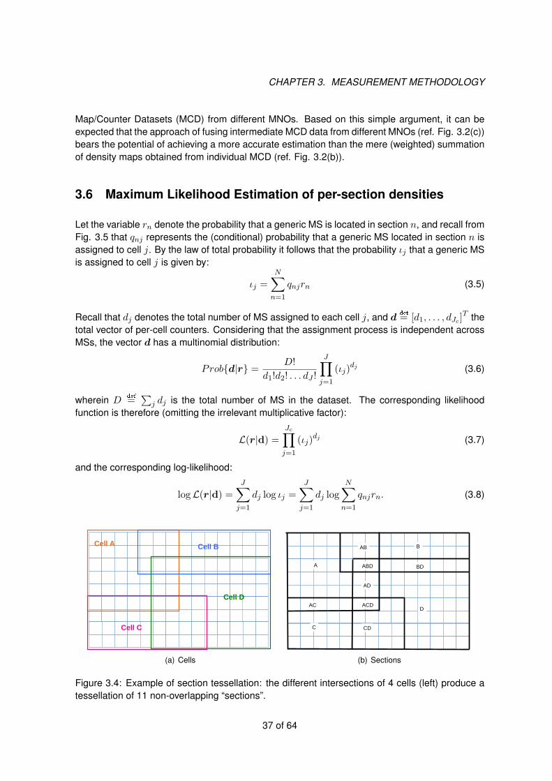
CHAPTER 3. MEASUREMENT METHODOLOGY
Map/Counter Datasets (MCD) from different MNOs. Based on this simple argument, it can beexpected that the approach of fusing intermediate MCD data from different MNOs (ref. Fig. 3.2(c))bears the potential of achieving a more accurate estimation than the mere (weighted) summationof density maps obtained from individual MCD (ref. Fig. 3.2(b)).
3.6 Maximum Likelihood Estimation of per-section densities
Let the variable rn denote the probability that a generic MS is located in section n, and recall fromFig. 3.5 that qnj represents the (conditional) probability that a generic MS located in section n isassigned to cell j. By the law of total probability it follows that the probability ιj that a generic MSis assigned to cell j is given by:
ιj =N∑n=1
qnjrn (3.5)
Recall that dj denotes the total number of MS assigned to each cell j, and ddef
= [d1, . . . , dJc ]T the
total vector of per-cell counters. Considering that the assignment process is independent acrossMSs, the vector d has a multinomial distribution:
Probd|r =D!
d1!d2! . . . dJ !
J∏j=1
(ιj)dj (3.6)
wherein Ddef
=∑
j dj is the total number of MS in the dataset. The corresponding likelihoodfunction is therefore (omitting the irrelevant multiplicative factor):
L(r|d) =
Jc∏j=1
(ιj)dj (3.7)
and the corresponding log-likelihood:
logL(r|d) =
J∑j=1
dj log ιj =
J∑j=1
dj log
N∑n=1
qnjrn. (3.8)
Cell A Cell B
Cell D
Cell C
(a) Cells
A
AB B
BD ABD
AD
ACD AC
C CD
D
(b) Sections
Figure 3.4: Example of section tessellation: the different intersections of 4 cells (left) produce atessellation of 11 non-overlapping “sections”.
37 of 64

CHAPTER 3. MEASUREMENT METHODOLOGY
In the considered setting, we have four types of spatial entities: tiles, cells, LAs and sections.Hererby, we distinguish between indices for each type of spatial entity, and ways to encodethe associations (mapping) between different types. We shall use vectorial notation toencode the cell-to-tile mapping, and set notation for the other mappings.
The symbols K,J,N,L denote the total number of tiles, cells, sections and LA, respectively.We shall use a distinct index for every type of object:
• k = 1, . . . ,K the tile index.
• j = 1, . . . , J the cell index.
• n = 1, . . . , N the section index
• ` = 1, . . . , L the LA index.
Mappings and associated quantities:
• bkj ∈ 0, 1 boolean variable indicating whether tile k is included in cell j footprint.
• bjdef
= [b1j , . . . , bKj ]T the boolean vector representing the map of cell j.
• βjdef
=∑
k bkj the size of cell j on the reference grid, i.e., the number of tiles spannedby cell j footprint.
• A` the set of cells included in LA `.
• Vn the set of tiles included in section n and vndef
= |Vn| the size of section n.
• Zn the set of cells defining section n and zndef
= |Zn| the number thereof.
• qnjdef
=
z−1n if j ∈ Zn,0 if j /∈ Zn.
a set of model parameters derived from the cell coverage
pattern. More in detail, qnj ∈ [0, 1] represents the probability that a generic MS insection n is assigned to cell j in the generative model described in Appendix A.
Variables and parameters:
• cj and c` the number of MS observed in cell j and LA `, respectively.
• dj the MS counter for cell j after projection of LA counters (ref §3.4)
• D def
=∑
j dj the total number of MS observed in the whole network.
• γ ∈ [0, 1] a tunable parameter in the LA projection procedure described in §3.4.
• xk the (unknown) number of MS in tile k and xk the final estimated value obtained withthe procedure described in §3.6.
Figure 3.5: Notation used in the presentation of the estimation method.
38 of 64

CHAPTER 3. MEASUREMENT METHODOLOGY
Therefore the Maximum Likelihood (ML) estimate r given the data d and the model qnj is givenby the solution of the following constrained optimization:
maximizeJ∑j=1
dj log
N∑n=1
qnjrn
subject toN∑n=1
rn = 1,
rn ≥ 0, ∀n,
(3.9)
or, equivalently, to find:
r = arg maxr≥0‖r‖1=1
J∑j=1
dj log
N∑n=1
qnjrn. (3.10)
3.7 Deriving per-tile estimates
The solution r to (3.10) represent the estimate of (normalised) per-section counters. For everytile k ∈ Vn in section n we derive a preliminary per-tile estimate by simply distributing of theper-section value uniformly across the component tiles, and rescaling by D, formally:
uk =rnD
vn, ∀k ∈ Vn, ∀n (3.11)
wherein vn denotes the size (in number of tiles) of section n. Finally, a simple 2D smoothing filter(e.g. circular gaussian) is run on the values of uk in order to soften the artefactual discontinuitiesintroduced by the hard-boundary tessellation, formally:
x = Su (3.12)
wherein S denotes the smoothing matrix.
39 of 64
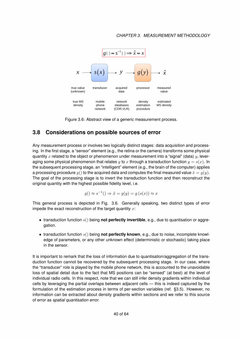
CHAPTER 3. MEASUREMENT METHODOLOGY
xs x( ) g y( )yx
true value (unknown)
transducer acquired data
processor measured value
true MS density
mobile phone
network
network databases (CDR,VLR)
density estimation procedure
estimated MS density
g ( ) ≈ s−1 ( )⇒ x ≈ x
Figure 3.6: Abstract view of a generic measurement process.
3.8 Considerations on possible sources of error
Any measurement process or involves two logically distinct stages: data acquisition and process-ing. In the first stage, a “sensor” element (e.g., the retina or the camera) transforms some physicalquantity x related to the object or phenomenon under measurement into a “signal” (data) y, lever-aging some physical phenomenon that relates y to x through a transduction function y = s(x). Inthe subsequent processing stage, an “intelligent” element (e.g., the brain of the computer) appliesa processing procedure g() to the acquired data and computes the final measured value x = g(y).The goal of the processing stage is to invert the transduction function and then reconstruct theoriginal quantity with the highest possible fidelity level, i.e.
g() ≈ s−1()⇒ x = g(y) = g (s(x)) ≈ x
This general process is depicted in Fig. 3.6. Generally speaking, two distinct types of errorimpede the exact reconstruction of the target quantity x:
• transduction function s() being not perfectly invertible, e.g., due to quantisation or aggre-gation.
• transduction function s() being not perfectly known, e.g., due to noise, incomplete knowl-edge of parameters, or any other unknown effect (deterministic or stochastic) taking placein the sensor.
It is important to remark that the loss of information due to quantisation/aggregation of the trans-duction function cannot be recovered by the subsequent processing stage. In our case, wherethe “transducer” role is played by the mobile phone network, this is accounted to the unavoidableloss of spatial detail due to the fact that MS positions can be “sensed” (at best) at the level ofindividual radio cells. In this respect, note that we can still infer density gradients within individualcells by leveraging the partial overlaps between adjacent cells — this is indeed captured by theformulation of the estimation process in terms of per-section variables (ref. §3.5). However, noinformation can be extracted about density gradients within sections and we refer to this sourceof error as spatial quantisation error.
40 of 64
CHAPTER 3. MEASUREMENT METHODOLOGY
In more concrete terms, the amount of information loss due to spatial quantisation depends(among other factors) on the particular network configuration, and particularly on the radio cover-age patterns, i.e., location and size of radio cells. For this reason, different MNO networks mightbe “sensing” the same population with different levels of accuracy, and the network of the sameMNO might yield different accuracy in different areas.
From the perspective of the population density estimation process, the “transducer” (i.e., themobile phone network infrastructure) is given and cannot be changed. In other words, the spatialquantisation error represents an irreducible error floor for any network-based estimation method.
Besides that, our knowledge of the transduction function is not perfect, and this results in anadditional source of error during the data processing stage which we call estimation error. Thisis due to several factors, most prominently: (i) a certain number of simplifying assumptions inthe modelling of the network dynamics, hence in the “model” of the transduction function to beinverted; (ii) coarsely approximated knowledge of the real cell footprints (i.e., the area effectivelyserviced by a cell site); (iii) stochastic fluctuations (e.g., due to the wireless channel randomness)and (iv) spurious correlations between the transduction process and the phenomenon under ob-servation. The latter is particularly insidious as it introduces a systematic distortion (or bias) inthe final estimate.
Hereafter we provide a list of the main sources of errors that affect the estimation method pre-sented in this Chapter.
• Inaccurate knowledge of cell coverage area: it is reasonable to expect that only a verycoarse approximation of the cell footprint is available to the MNO, due to the intrinsic com-plexity and variability of the radio propagation channel.
• M2M devices: as discussed earlier in §1.6, the presence of MS for machine-to-machine(M2M) communications may inflate the MS counters and therefore lead to an over-estimationof population density. The problem will become more serious in the future, due to the ex-pected growth of M2M devices served by mobile networks (“Internet of Things” paradigm).The problem can be counteract by applying more sophisticated M2M identification and pre-filtering routines already in the data collection stage, but unavoidably the implementation ofthese routines will be highly MNO-specific.
• Biased cell-level location data: as discussed earlier in §3.3, the generation of cell-levellocations data is conditioned to the occurrence of certain events (phone call, SMS, dataconnection, signalling procedure) related to the MS activity pattern. Since MS activity is notindependent from time and space, the probability that the MS location is “observed” (sam-pled) at cell-level is correlated with the location itself (and with time). This in general leadsto possible distortions in the final estimation, i.e., over- or under-representation of certain lo-cations at certain times. Note that (at least part of) such correlations are systematic acrossdifferent MNOs, and therefore can be perhaps mitigated but not completely eliminated byfusing data from diverse MNOs.
• MNO-specific customer base: the network infrastructure of a generic MNO can observeonly part of the total population, and specifically (i) the customers of the MNO itself and(ii) customers of other MNO roaming into this network. In other words, every MNO “sam-ples” part of the population, i.e., it can observe only a subset of all population members.
41 of 64

CHAPTER 3. MEASUREMENT METHODOLOGY
Note that the same person can be observed by two (or more) distinct MNOs if (s)he car-ries multiple subscriptions (e.g., a personal phone and a company phone). This leads toover-estimation of certain user groups (e.g., professionals), which demands systematic cor-rections. Besides duplications, attention must be paid to the fact that the customer basecomposition in general differs across MNOs. This introduces distortion (bias) representa-tion of groups, among the subscribers of each individual MNO4. However such a bias canbe reduced by jointly analysing data from different — possibly all — MNOs within the samemarket (country).
In principle, one can seek to reduce the estimation error by developing more sophisticated esti-mation algorithms based on more accurate (and complex) models of MS-to-network interactionsand/or by leveraging external information from other systems. The quantitative assessment of theactual magnitude of these errors in real-world data remains a central direction for future research.
4Consider for example two MNOs m1 and m2 that are preferred, respectively, by low-income and high-incomeprofessionals. This “market specialisation” will cause luxury residential areas to be under-represented in m1’s dataand over-represented in m2’s data.
42 of 64
Chapter 4
Exemplary Results with Synthetic data
This section provides numerical results for a simplified synthetic scenario. The main goal is tovalidate the correctness of the proposed method, and specifically the consistency of the maximumlikelihood (ML) estimation method described in §3.6, and at the same time illustrate visually thetype of outcome that can be expected. The simulation results presented hereafter represent thestarting point for a future in-depth analysis of the performances, complexity and, most prominently,sensitivity of the proposed method to several real-world situations and potential sources of errorsencountered in practice. In this sense, we do not aim here at reproducing each and every aspectof a “realistic” real-world scenario — a task that we leave for future work — but merely to illustratethe correctness of our approach in a simplified, reasonably well-behaved synthetic scenario.
4.1 Description of simulation scenario
We consider a network consisting of a square grid of 100 × 100 tiles hosting a total of 650, 000MS. The MS are distributed randomly according to a bivariate distribution consisting of a mixtureof three distinct Gaussian clusters, as shown in the “ground truth” map of Fig. 4.2(a).
We consider three types of cells with different footprint size and shape: (i) small sectors with 120
beam, (ii) medium-size circular cells and (iii) large circular cells. Note that three neighbouring120-sectors share the same cell tower. Cells are placed randomly according to an arbitrarydesign process that favour placement of more and smaller cells in most densely populated areas.This reflects the characteristic of real-world deployments, where the spatial distribution of radiocapacity (i.e., more and smaller cells) tend to follows the maximum traffic intensity (peak-hourtraffic), and therefore correlates positively with the (maximum) population density.
We consider two distinct scenarios (Scenario #1 and Scenario #2) with two different cell coveragepatterns extracted randomly from the same process. For Scenario #2 we manually modified thecell placement in order to introduce a strong local mismatching in a particular region, as explainedin detail later in §4.3.2.
The number of simulated cells is 56 for Scenario #1 and 117 for Scenario #2. In each scenario,cells are arbitrarily grouped into 5 simulated LAs of different size. An excerpt of the cell/LAfootprints in Scenario #1 is depicted in Fig. 4.1.
43
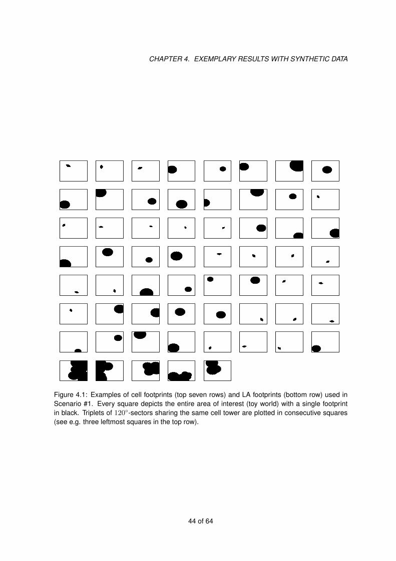
CHAPTER 4. EXEMPLARY RESULTS WITH SYNTHETIC DATA
Figure 4.1: Examples of cell footprints (top seven rows) and LA footprints (bottom row) used inScenario #1. Every square depicts the entire area of interest (toy world) with a single footprintin black. Triplets of 120-sectors sharing the same cell tower are plotted in consecutive squares(see e.g. three leftmost squares in the top row).
44 of 64
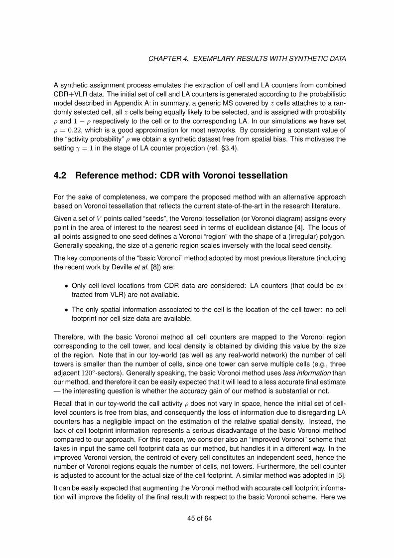
CHAPTER 4. EXEMPLARY RESULTS WITH SYNTHETIC DATA
A synthetic assignment process emulates the extraction of cell and LA counters from combinedCDR+VLR data. The initial set of cell and LA counters is generated according to the probabilisticmodel described in Appendix A: in summary, a generic MS covered by z cells attaches to a ran-domly selected cell, all z cells being equally likely to be selected, and is assigned with probabilityρ and 1 − ρ respectively to the cell or to the corresponding LA. In our simulations we have setρ = 0.22, which is a good approximation for most networks. By considering a constant value ofthe “activity probability” ρ we obtain a synthetic dataset free from spatial bias. This motivates thesetting γ = 1 in the stage of LA counter projection (ref. §3.4).
4.2 Reference method: CDR with Voronoi tessellation
For the sake of completeness, we compare the proposed method with an alternative approachbased on Voronoi tessellation that reflects the current state-of-the-art in the research literature.
Given a set of V points called “seeds”, the Voronoi tessellation (or Voronoi diagram) assigns everypoint in the area of interest to the nearest seed in terms of euclidean distance [4]. The locus ofall points assigned to one seed defines a Voronoi “region” with the shape of a (irregular) polygon.Generally speaking, the size of a generic region scales inversely with the local seed density.
The key components of the “basic Voronoi” method adopted by most previous literature (includingthe recent work by Deville et al. [8]) are:
• Only cell-level locations from CDR data are considered: LA counters (that could be ex-tracted from VLR) are not available.
• The only spatial information associated to the cell is the location of the cell tower: no cellfootprint nor cell size data are available.
Therefore, with the basic Voronoi method all cell counters are mapped to the Voronoi regioncorresponding to the cell tower, and local density is obtained by dividing this value by the sizeof the region. Note that in our toy-world (as well as any real-world network) the number of celltowers is smaller than the number of cells, since one tower can serve multiple cells (e.g., threeadjacent 120-sectors). Generally speaking, the basic Voronoi method uses less information thanour method, and therefore it can be easily expected that it will lead to a less accurate final estimate— the interesting question is whether the accuracy gain of our method is substantial or not.
Recall that in our toy-world the call activity ρ does not vary in space, hence the initial set of cell-level counters is free from bias, and consequently the loss of information due to disregarding LAcounters has a negligible impact on the estimation of the relative spatial density. Instead, thelack of cell footprint information represents a serious disadvantage of the basic Voronoi methodcompared to our approach. For this reason, we consider also an “improved Voronoi” scheme thattakes in input the same cell footprint data as our method, but handles it in a different way. In theimproved Voronoi version, the centroid of every cell constitutes an independent seed, hence thenumber of Voronoi regions equals the number of cells, not towers. Furthermore, the cell counteris adjusted to account for the actual size of the cell footprint. A similar method was adopted in [5].
It can be easily expected that augmenting the Voronoi method with accurate cell footprint informa-tion will improve the fidelity of the final result with respect to the basic Voronoi scheme. Here we
45 of 64

CHAPTER 4. EXEMPLARY RESULTS WITH SYNTHETIC DATA
are interested to compare the improved Voronoi approach with the proposed estimation methodthat uses the same information — cell footprints and counters — but in a different way.
4.3 Numerical results
4.3.1 Scenario #1: a well-behaved case
The color map in Fig. 4.2(a) shows the “ground truth” distribution generated for Scenario #1,aggregated at the tile level (K =10,000 total tiles). The three clusters A, B and C are evident.
Identification of reference bound
Fig. 4.2(b) shows the ground truth distribution aggregated at section level — recall that everysection represents the intersection area of a specific subset of cells. After passing the latterthrough a smoothing filter we obtain the map in Fig. 4.2(b), which represents the output (aftersmoothing) of an ideal “oracle” that knows without error the ground truth distribution at the levelof individual sections. In other words, moving from the per-tile ground truth of Fig. 4.2(a) to themap in Fig. 4.2(c) has introduced exclusively a spatial aggregation error but no estimation error.It is important to realise that the spatial aggregation error (at per-section level) is intrinsic to theusage of the mobile phone network, and specifically of network-based data, for the detectionof MS locations: the unavoidable loss of spatial detail is due to the fact that MS locations canbe “sensed” (at best) at the level of individual radio cell. For this reason, given a radio networkcoverage pattern (i.e., the given set of cell footprints) and without any further external information,the “oracle” map in Fig. 4.2(c) represents the ideal reference bound against which any densityestimation method based on network data must be compared.
Output of the proposed method
In Fig. 4.2(d) we report the density map obtained by the ML estimation procedure described in§3.6. Moving from Fig. 4.2(c) to (4.2(d)) a certain estimation error has been introduced. Thecomparison between the two maps shows that the quality of the final estimate is rather good: allthree clusters are clearly distinguishable. Note that while cluster C (upper left) has been slightlyfaded out, the cluster B (lower left) has been resolved very accurately. Such differences are dueto the local coverage pattern in the cluster region: the more redundant the local coverage (highernumber and smaller size of cells) the better the estimation accuracy.
Comparison with Voronoi schemes
In Fig. 4.3 we plot the results obtained by the two Voronoi schemes. As expected, the injection ofcell footprint information improves somewhat the performance of the improved Voronoi approachcompared with the basic Voronoi (compare Fig. 4.3(c) against Fig. 4.3(b)), but in both cases theresult is considerably less accurate than the proposed method. This is further confirmed by thedistribution of the absolute errors plotted in Fig. 4.4.
46 of 64
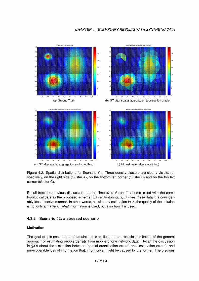
CHAPTER 4. EXEMPLARY RESULTS WITH SYNTHETIC DATA
10 20 30 40 50 60 70 80 90 100
10
20
30
40
50
60
70
80
90
100True population distribution
0
50
100
150
200
250
300
(a) Ground Truth
10 20 30 40 50 60 70 80 90 100
10
20
30
40
50
60
70
80
90
100True population distribution over Sections
0
50
100
150
200
250
300
(b) GT after spatial aggregation (per-section oracle)
10 20 30 40 50 60 70 80 90 100
10
20
30
40
50
60
70
80
90
100True population distribution over Sections (smoothed)
0
50
100
150
200
250
300
(c) GT after spatial aggregation and smoothing
10 20 30 40 50 60 70 80 90 100
10
20
30
40
50
60
70
80
90
100Estimation based on MaxLH (smoothed)
0
50
100
150
200
250
300
(d) ML estimate (after smoothing)
Figure 4.2: Spatial distributions for Scenario #1. Three density clusters are clearly visible, re-spectively, on the right side (cluster A), on the bottom left corner (cluster B) and on the top leftcorner (cluster C).
Recall from the previous discussion that the “improved Voronoi” scheme is fed with the sametopological data as the proposed scheme (full cell footprint), but it uses these data in a consider-ably less effective manner. In other words, as with any estimation task, the quality of the solutionis not only a matter of what information is used, but also how it is used.
4.3.2 Scenario #2: a stressed scenario
Motivation
The goal of this second set of simulations is to illustrate one possible limitation of the generalapproach of estimating people density from mobile phone network data. Recall the discussionin §3.8 about the distinction between “spatial quantisation errors” and “estimation errors”, andunrecoverable loss of information that, in principle, might be caused by the former. The previous
47 of 64
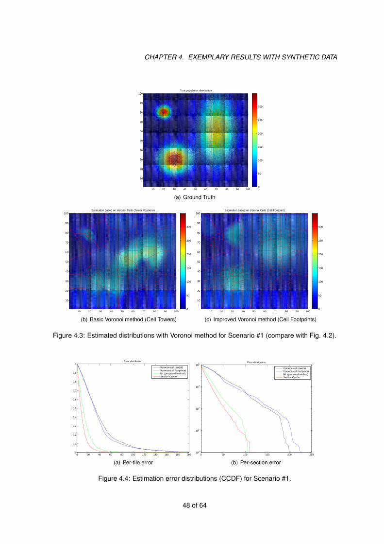
CHAPTER 4. EXEMPLARY RESULTS WITH SYNTHETIC DATA
10 20 30 40 50 60 70 80 90 100
10
20
30
40
50
60
70
80
90
100True population distribution
0
50
100
150
200
250
300
(a) Ground Truth
10 20 30 40 50 60 70 80 90 100
10
20
30
40
50
60
70
80
90
100Estimation based on Voronoi Cells (Tower Positions)
0
50
100
150
200
250
300
(b) Basic Voronoi method (Cell Towers)
10 20 30 40 50 60 70 80 90 100
10
20
30
40
50
60
70
80
90
100Estimation based on Voronoi Cells (Cell Footprint)
0
50
100
150
200
250
300
(c) Improved Voronoi method (Cell Footprints)
Figure 4.3: Estimated distributions with Voronoi method for Scenario #1 (compare with Fig. 4.2).
0 20 40 60 80 100 120 140 160 180 2000
0.1
0.2
0.3
0.4
0.5
0.6
0.7
0.8
0.9
1Error distribution
Voronoi (cell towers)Voronoi (cell footprints)ML (proposed method)Section Oracle
(a) Per-tile error
0 50 100 150 200 25010
−4
10−3
10−2
10−1
100
Error distribution
Voronoi (cell towers)Voronoi (cell footprints)ML (proposed method)Section Oracle
(b) Per-section error
Figure 4.4: Estimation error distributions (CCDF) for Scenario #1.
48 of 64
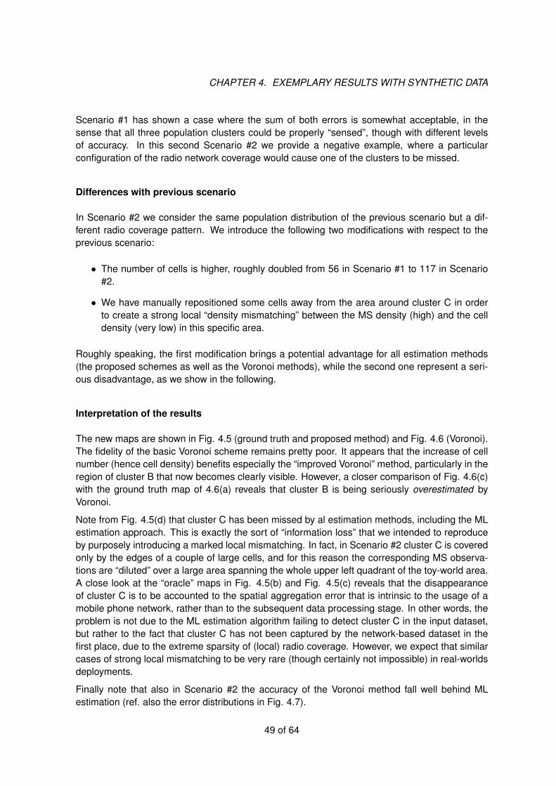
CHAPTER 4. EXEMPLARY RESULTS WITH SYNTHETIC DATA
Scenario #1 has shown a case where the sum of both errors is somewhat acceptable, in thesense that all three population clusters could be properly “sensed”, though with different levelsof accuracy. In this second Scenario #2 we provide a negative example, where a particularconfiguration of the radio network coverage would cause one of the clusters to be missed.
Differences with previous scenario
In Scenario #2 we consider the same population distribution of the previous scenario but a dif-ferent radio coverage pattern. We introduce the following two modifications with respect to theprevious scenario:
• The number of cells is higher, roughly doubled from 56 in Scenario #1 to 117 in Scenario#2.
• We have manually repositioned some cells away from the area around cluster C in orderto create a strong local “density mismatching” between the MS density (high) and the celldensity (very low) in this specific area.
Roughly speaking, the first modification brings a potential advantage for all estimation methods(the proposed schemes as well as the Voronoi methods), while the second one represent a seri-ous disadvantage, as we show in the following.
Interpretation of the results
The new maps are shown in Fig. 4.5 (ground truth and proposed method) and Fig. 4.6 (Voronoi).The fidelity of the basic Voronoi scheme remains pretty poor. It appears that the increase of cellnumber (hence cell density) benefits especially the “improved Voronoi” method, particularly in theregion of cluster B that now becomes clearly visible. However, a closer comparison of Fig. 4.6(c)with the ground truth map of 4.6(a) reveals that cluster B is being seriously overestimated byVoronoi.
Note from Fig. 4.5(d) that cluster C has been missed by al estimation methods, including the MLestimation approach. This is exactly the sort of “information loss” that we intended to reproduceby purposely introducing a marked local mismatching. In fact, in Scenario #2 cluster C is coveredonly by the edges of a couple of large cells, and for this reason the corresponding MS observa-tions are “diluted” over a large area spanning the whole upper left quadrant of the toy-world area.A close look at the “oracle” maps in Fig. 4.5(b) and Fig. 4.5(c) reveals that the disappearanceof cluster C is to be accounted to the spatial aggregation error that is intrinsic to the usage of amobile phone network, rather than to the subsequent data processing stage. In other words, theproblem is not due to the ML estimation algorithm failing to detect cluster C in the input dataset,but rather to the fact that cluster C has not been captured by the network-based dataset in thefirst place, due to the extreme sparsity of (local) radio coverage. However, we expect that similarcases of strong local mismatching to be very rare (though certainly not impossible) in real-worldsdeployments.
Finally note that also in Scenario #2 the accuracy of the Voronoi method fall well behind MLestimation (ref. also the error distributions in Fig. 4.7).
49 of 64

CHAPTER 4. EXEMPLARY RESULTS WITH SYNTHETIC DATA
10 20 30 40 50 60 70 80 90 100
10
20
30
40
50
60
70
80
90
100True population distribution
0
50
100
150
200
250
300
350
(a) Ground Truth (GT)
10 20 30 40 50 60 70 80 90 100
10
20
30
40
50
60
70
80
90
100True population distribution over Sections
0
50
100
150
200
250
300
350
(b) GT after spatial aggregation (per-section oracle)
10 20 30 40 50 60 70 80 90 100
10
20
30
40
50
60
70
80
90
100True population distribution over Sections (smoothed)
0
50
100
150
200
250
300
350
(c) GT after spatial aggregation and smoothing
10 20 30 40 50 60 70 80 90 100
10
20
30
40
50
60
70
80
90
100Estimation based on MaxLH (smoothed)
0
50
100
150
200
250
300
350
(d) ML estimate (after smoothing)
Figure 4.5: Spatial density maps for Scenario #2. Note that Cluster C is missing already in the“oracle” map due to the particularly “low” degree of radio coverage in that area. Consequently,Cluster C is missed also by the final ML estimate)
50 of 64

CHAPTER 4. EXEMPLARY RESULTS WITH SYNTHETIC DATA
10 20 30 40 50 60 70 80 90 100
10
20
30
40
50
60
70
80
90
100True population distribution
0
50
100
150
200
250
300
350
(a) Ground Truth
10 20 30 40 50 60 70 80 90 100
10
20
30
40
50
60
70
80
90
100Estimation based on Voronoi Cells (Tower Positions)
0
50
100
150
200
250
300
350
(b) Basic Voronoi method (Cell Towers)
10 20 30 40 50 60 70 80 90 100
10
20
30
40
50
60
70
80
90
100Estimation based on Voronoi Cells (Cell Footprint)
0
50
100
150
200
250
300
350
(c) Improved Voronoi method (Cell Footprints)
Figure 4.6: Estimated density maps with Voronoi method for Scenario #2 (compare with Fig. 4.5).
0 20 40 60 80 100 120 140 160 180 2000
0.1
0.2
0.3
0.4
0.5
0.6
0.7
0.8
0.9
1Error distribution
Voronoi (cell towers)Voronoi (cell footprints)ML (proposed method)Section Oracle
(a) Per-tile error
0 50 100 150 200 250 30010
−4
10−3
10−2
10−1
100
Error distribution
Voronoi (cell towers)Voronoi (cell footprints)ML (proposed method)Section Oracle
(b) Per-section error
Figure 4.7: Estimation error distributions (CCDF) for Scenario #2.s
51 of 64
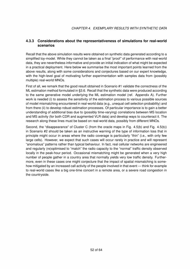
CHAPTER 4. EXEMPLARY RESULTS WITH SYNTHETIC DATA
4.3.3 Considerations about the representativeness of simulations for real-worldscenarios
Recall that the above simulation results were obtained on synthetic data generated according to asimplified toy-model. While they cannot be taken as a final “proof” of performance with real-worlddata, they are nevertheless informative and provide an initial indication of what might be expectedin a practical deployment. Here below we summarise the most important points learned from theabove results, along with some considerations and conjectures based on our expert knowledge,with the high-level goal of motivating further experimentation with samples data from (possiblymultiple) real-world MNOs.
First of all, we remark that the good result obtained in Scenario #1 validate the correctness of theML estimation method formulated in §3.6. Recall that the synthetic data were produced accordingto the same generative model underlying the ML estimation model (ref. Appendix A). Furtherwork is needed (i) to assess the sensitivity of the estimation process to various possible sourcesof model mismatching encountered in real-world data (e.g., unequal cell selection probability) andfrom there (ii) to develop robust estimation processes. Of particular importance is to gain a betterunderstanding of additional bias due to (possibly time-varying) correlations between MS locationand MS activity (for both CDR and augmented VLR data) and develop ways to counteract it. Theresearch along these lines must be based on real-world data, possibly from different MNOs.
Second, the “disappearance” of Cluster C (from the oracle maps in Fig. 4.5(b) and Fig. 4.5(b))in Scenario #2 should be taken as an instructive warning of the type of information loss that inprinciple might occur in areas where the radio coverage is particularly “thin” (i.e., with only fewlarge cells). However, we expect that such cases will occur rarely in practice and will represent“anomalous” patterns rather than typical behaviour. In fact, real cellular networks are engineeredand regularly (re)optimised to “match” the radio capacity to the “normal” traffic density observedlocally in the peak-hour period. Occasional mismatching might be generated when a very highnumber of people gather in a country area that normally yields very low traffic density. Further-more, even in these cases one might conjecture that the impact of spatial mismatching is some-how mitigated by an increased call activity of the people involved in that event — think for exampleto real-world cases like a big one-time concert in a remote area, or a severe road congestion inthe countryside.
52 of 64
Chapter 5
Summary of main findings and pointsfor further study
In this chapter, we summarise the main results of this study and we point out promising directionsfor future work.
Importance of better network topology data
The simulation results in Chapter 4 indicate that major gains in estimation accuracy can be ob-tained by integrating mobile operator data with additional topology data. For example, the densityestimation procedure (and likely any other spatial analysis based on mobile phone data) wouldgreatly benefit from the use of accurate cell coverage maps. Now, while cell coverage mapsare measured or estimated at great computational costs, coarse approximations are in generalavailable. In addition, any coarse approximation of cell footprint (e.g. obtained by static antennaconfiguration parameters) improves the data location resolution of mere (exact) tower location,and the simulation results presented in this study support this claim. As MNO typically possessthis information, we propose to implement internal processes so as to prepare cell coverage datafor their use in combination with CDR/VLR data for improved spatial analysis. Note also that,when cell coverage maps are made available, the (inter-)section tessellation defined in this studycan greatly improve the results obtained by assuming a Voronoi tessellation method.
Understanding and quantifying the risk of spatial bias
In this work, we have often commented on cell-level location data being exposed to the risk ofspatial estimation uncertainty (or bias). In fact, due to the functional dynamics of the mobile phonenetwork, the estimation of a cell location is always conditioned to the event of a subscriber startinga phone call or sending an SMS, whose probability of occurrence typically depends on the MS’scontext and location. Furthermore, the correlation structure between MS location and MS activitymight be varying with time. This introduces a certain risk of under- or over-representing certainspecific locations in cell-level data, leading to distorted view of the population distribution in spaceand/or time.
53

CHAPTER 5. SUMMARY OF MAIN FINDINGS AND POINTS FOR FURTHER STUDY
Notably, the problem lies exclusively in cell-level location data (both from CDR and augmentedVLR), i.e., it is contained at a small scale. For this reason, we conjecture the existence of a fun-damental trade-off between spatial accuracy and risk of bias — a phenomenon that is somewhatreminiscent of the bias-variance trade-off in statistics and machine learning [11].
Hence, additional work is required for a better understanding of the various sources of spa-tial/temporal bias in real MNO dataset, and to quantify the resulting distortion in the final densityestimation. In this respect, the complexity of this task is aggravated by the fact that reference“ground truth"data might not be available in practice, and that it might be necessary to resortto comparative studies across different MNO, with different network configurations and customerpopulation characteristics. Nevertheless, the integration of dataset from different operators (e.g.,on the basis of joint pilot studies, or projects) is deemed as a promising strategy for reducinguncertainty and obtain accurate estimations.
Counteracting the risk of bias
Another important challenge is to develop effective approaches to counteract the spatial/temporalbias that is possibly present in cell-level data. The adoption of adjustable parameters, such as γ in§3.4 should be considered as a very simple initial attempt to address such a problem. Alternativeapproaches might consider calibration strategies based on reference data (e.g., census data [8])or leveraging external data (e.g. land use), which, however, require additional countermeasuresto prevent error propagation across datasets.
Quantifying the cost and benefit of VLR data
Numerous case-studies investigating CDR applications demonstrate that the effort required forthe extraction and preparation of such data is affordable for many MNOs. Unfortunately, there isno indication about the feasibility (and costs) of large-scale extraction of VLR data, nor about theachievable gains (e.g., in terms of population coverage, reduced bias, temporal resolution) thatVLR data can bring to the task of population density estimation. As a result, further experimentalwork is required to quantify the cost and the potential benefits of complementing CDR with VLRdata. The intention of this study was to provide a unified methodological basis for the joint pro-cessing of cell-level and LA-level data, hence for the fusion of CDR and VLR, and to shed light onthe opportunity of network data exploration besides traditional CDR data sets.
Towards a multi-MNO pilot study
A number of research directions identified during this study would involve the fusion of, or atleast the comparison between, network-based data extracted by different MNOs. We do notrefer here to “raw" CDR/VLR data nor any other type of micro-data — that in our data process-ing model never leave the MNO domain — but to highly-aggregated intermediate data: preferablyMap/Counter Dataset (MCD), or at least density maps (ref. §3.1). In order to pioneer the joint pro-cessing of multi-MNO dataset we envision the launch of pilot projects involving different MNOs forthe coordinated extraction of sample datasets to be further processed and analysed by a trustedentity (e.g. JRC or Eurostat). It would be highly desirable to involve in the pilot study at least
54 of 64
CHAPTER 5. SUMMARY OF MAIN FINDINGS AND POINTS FOR FURTHER STUDY
two or three MNOs competing on the same national market. This would allow the investigationof the relative differences in the individual MNO’s “views" (due to different network configurationsand customer basis) as well as the quantitative assessment of the relative gain — in terms ofspatial accuracy and/or bias mitigation — achieved by the two multi-MNO data fusion strategiespresented in §3.1, namely MCD fusion vs. individual map fusion.
We expect that several European MNOs will favourably consider the perspective of engaging ina common multi-MNO pilot study, simply by considering it as an opportunity cost. Hereby, theefforts for the preparation of a sample dataset (e.g., CDR plus cell topology data) to serve asinput for the pilot study will probably not exceed a few person-months, considering that suchdata are anyway available inside MNOs — still they need to be properly prepared, curated andpre-processed. Among expected benefits, there is a growing consensus among MNOs on thecommercial value of the data in their possess, and the federation of multi-MNO data — at leastwithin the limited scope of a pilot project — bears the potential to stimulate new applications,attract new customers that are not at reach of individual MNOs, as well as European institutionssupporting public policies. We hope this study will contribute concretely to move some steps inthis direction.
—————————–
55 of 64
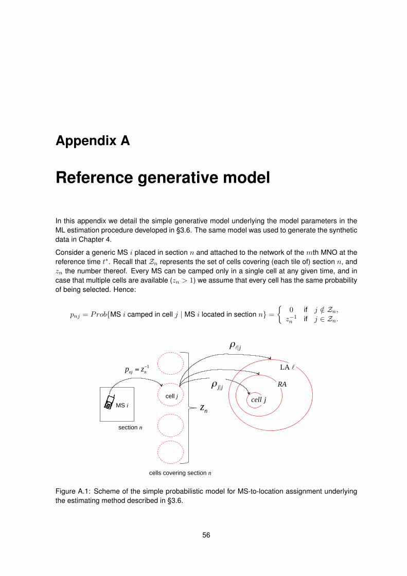
Appendix A
Reference generative model
In this appendix we detail the simple generative model underlying the model parameters in theML estimation procedure developed in §3.6. The same model was used to generate the syntheticdata in Chapter 4.
Consider a generic MS i placed in section n and attached to the network of the mth MNO at thereference time t∗. Recall that Zn represents the set of cells covering (each tile of) section n, andzn the number thereof. Every MS can be camped only in a single cell at any given time, and incase that multiple cells are available (zn > 1) we assume that every cell has the same probabilityof being selected. Hence:
pnj = ProbMS i camped in cell j | MS i located in section n =
0 if j /∈ Zn,z−1n if j ∈ Zn.
MS i
section n
zn
cells covering section n
pnj = zn−1
cell j
ρ| j
LA
RAρ j| j
cell j
Figure A.1: Scheme of the simple probabilistic model for MS-to-location assignment underlyingthe estimating method described in §3.6.
56

APPENDIX A. REFERENCE GENERATIVE MODEL
The fact that MS i was camping to cell j is a necessary but not sufficient condition for i to be“observed" in cell j by the network measurement process. More precisely, MS i can be assignedto three different locations: the cell j itself (in the best case), the associated RA or the greater LA(in the worst case), as depicted in Fig. A.1. In practice, several factors concur to determine themapping area for MS i: (i) which source databases are considered by the measurement process(CDR and/or VLR); (ii) the configuration of the MS (e.g., whether it is attached exclusively to theCS domain or to the PS domain too) and (iii) the recent activity pattern of the MS (e.g., whether ithas performed voice calls in the reference observation interval). As discussed earlier in §3.3, theMS activity is not independent from the current MS location, and this introduce a certain risk ofbias, due to possible over- or under-representation of specific locations. In the simple generativemodel we disregard these types of correlations.
Formally, consider a cell j included in LA `, i.e., j ∈ A`. Denote by ρn ≤ 1 the activity coefficientin section n, i.e.
ρndef
= ProbMS i active | MS i located in section n.
By assuming that every MS is observed either in the respective cell of LA (for the sake of simplicitywe do not consider RA here), it holds that:
q′njdef
=ProbMS i observed in cell j | MS i located in section n=ProbMS i observed in cell j | MS i camped in cell j, located in section n·ProbMS i camped in cell j | MS i located in section n
=ρnpnj .
In the simple generative model we assume an uniform activity coefficient, i.e:
ρn = ρ, ∀n. (A.1)
With this simplifying assumption, the optimal value of the projection factor is γ = 1 (ref. §3.4),and therefore the probability that a generic MS located in section n is mapped to the (projected)counter dj reduces to qnj = pnj .
57 of 64

Appendix B
Preliminary analysis of LA sizes fromOpenCellID database
The mobile network can track the position of all MSs in active or idle mode at least at the levelof Location Areas (see Sect. 1). Moreover, although the position of active MSs is known atcell level, this information is not necessarily included in the VLR. This section aims to provide arough estimation of the spatial granularity of localizations at LA level based on a large dataset ofconcurrent GPS position and Cell-ID (equivalently: CGI) recordings. Such a dataset is providedfree of charge by OpenCellID [2].
The OpenCellID database
OpenCellID is a large collaborative project collecting GPS location data for cell identifiers (Cell-ID), with the main application of providing power-efficient and fast location information to mobiledevices. As of August 2014, over a billion measurements were collected, which are publiclyavailable under a free Creative Commons license [2]. The data is collected fully automaticallyby registered users via various smart phone apps. Although this database is primarily intendedto provide a mapping from given cell ids to geo-locations, we use it in this study to estimate thelocalization error - i.e. the spatial granularity - of device localizations based on cells or LocationAreas.
However, since OpenCellID data are collected by volunteers, compiled automatically and pro-vided free of charge, there is no guarantee regarding the quality of the data. Typical errors in theOpenCellId database include
• Erroneous cell-IDs: occasionally the recorded cell ids are wrong. Typically in these cases,the cell id, local area code (LAC) and mobile network code (MNC) are mixed up. In practice,the erroneous cell-IDs do have only few GPS measurements attached and can be easilyfiltered out by introducing a threshold to the number of measurement records for each cell.
• Unrealistic cell sizes: The GPS measurements of some cells are distributed across a wholecountry which is clearly unrealistic. The reason for this type of errors is not known to theauthors. One possible explanation for such phenomena are so-called “Cell-On-Wheels"
58

APPENDIX B. PRELIMINARY ANALYSIS OF LA SIZES FROM OPENCELLID DATABASE
(COW) or “Cell In A Box" (CIAB). These mobile antennas are used by MNOs to providetemporary service with temporary equipment, e.g. to cover increased demand at specificevents. Since mobile antennas can change their position and covered area, their ID willbe attached to GPS measurements which vary greatly over time and can yield a distortedpicture of actual cell sizes.
• “Antenna dragging": This type of data artifact seems to be caused by devices not updatingthe cell id during a trip, reporting the original cell id throughout and wrongly attaching it toGPS measurements.
• Outliers: Often, antennas with a number of plausible and consistent measurement pointshave additional GPS positions attached that are far away from the other measurements andare obviously wrong (often they are often not even in the same country).
Moreover, dependencies between measurements collected by the same contributor can intro-duce distortions, but the OpenCellID database does not include any identifier of the device northe person having collected the GPS and cell measurements. Robustly estimating LA sizes fromthe OpenCellID data in the presence of such errors and biases therefore involves an initial prepro-cessing step for data cleansing, and remaining noise is coped with by employing robust statisticsto analyse the spatial extents of cells and LAs.
Analysis method
To alleviate biases towards “heavy contributors” and dependencies between successive mea-surements during a trip or repeated measurements at the same location, we apply the followingfiltering scheme:
• for each cell in the mobile network only one measurement per hour is retained, and alladditional measurements are discarded;
• in a spatial 10m-by-10m grid only one measurement per grid-cell is retained, and all addi-tional measurements are discarded.
Furthermore, cells and LAs with too few measurements are not included in the analysis:
• Cells with less than 20 retained measurements are discarded;
• LAs with less than 10 different cells having a sufficient number of measurements are ex-cluded from analysis.
For the remaining Location Areas we define a robust centroid using only the retained measure-ments. While the median is a common robust measure for one-dimensional location, it does notgeneralize easily to higher dimensions. Several such generalizations are known [7], and for ouranalyses we use the centerpoint, which is defined as a point for which each hyperplane throughthe centerpoint divides the point cloud into two subsets such that the smaller of these subsetshas at least a 1
d+1 fraction of the points. The algorithm provided in [6] provides a fast probablisticapproach for computing centerpoints.
59 of 64
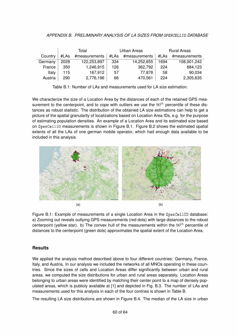
APPENDIX B. PRELIMINARY ANALYSIS OF LA SIZES FROM OPENCELLID DATABASE
Total Urban Areas Rural AreasCountry #LAs #measurements #LAs #measurements #LAs #measurements
Germany 2028 122,253,897 334 14,252,655 1694 108,001,242France 350 1,246,915 126 362,792 224 884,123
Italy 115 167,912 57 77,878 58 90,034Austria 290 2,776,196 66 470,561 224 2,305,635
Table B.1: Number of LAs and measurements used for LA size estimation.
We characterize the size of a Location Area by the distances of each of the retained GPS mea-surement to the centerpoint, and to cope with outliers we use the 90th percentile of these dis-tances as robust statistic. The distribution of the obtained LA size estimations can help to get apicture of the spatial granularity of localizations based on Location Area IDs, e.g. for the purposeof estimating population densities. An example of a Location Area and its estimated size basedon OpenCellID measurements is shown in Figure B.1. Figure B.2 shows the estimated spatialextents of all the LAs of one german mobile operator, which had enough data available to beincluded in this analysis.
(a) (b)
Figure B.1: Example of measurements of a single Location Area in the OpenCellID database:a) Zooming out reveals outlying GPS measurements (red dots) with large distances to the robustcenterpoint (yellow star). b) The convex hull of the measurements within the 90th percentile ofdistances to the centerpoint (green dots) approximates the spatial extent of the Location Area.
Results
We applied the analysis method described above to four different countries: Germany, France,Italy, and Austria. In our analysis we included the networks of all MNOs operating in these coun-tries. Since the sizes of cells and Location Areas differ significantly between urban and ruralareas, we computed the size distributions for urban and rural areas separately. Location Areasbelonging to urban areas were identified by matching their center point to a map of densely pop-ulated areas, which is publicly available at [1] and depicted in Fig. B.3. The number of LAs andmeasurements used for this analysis in each of the four contries is shown in Table B.
The resulting LA size distributions are shown in Figure B.4. The median of the LA size in urban
60 of 64
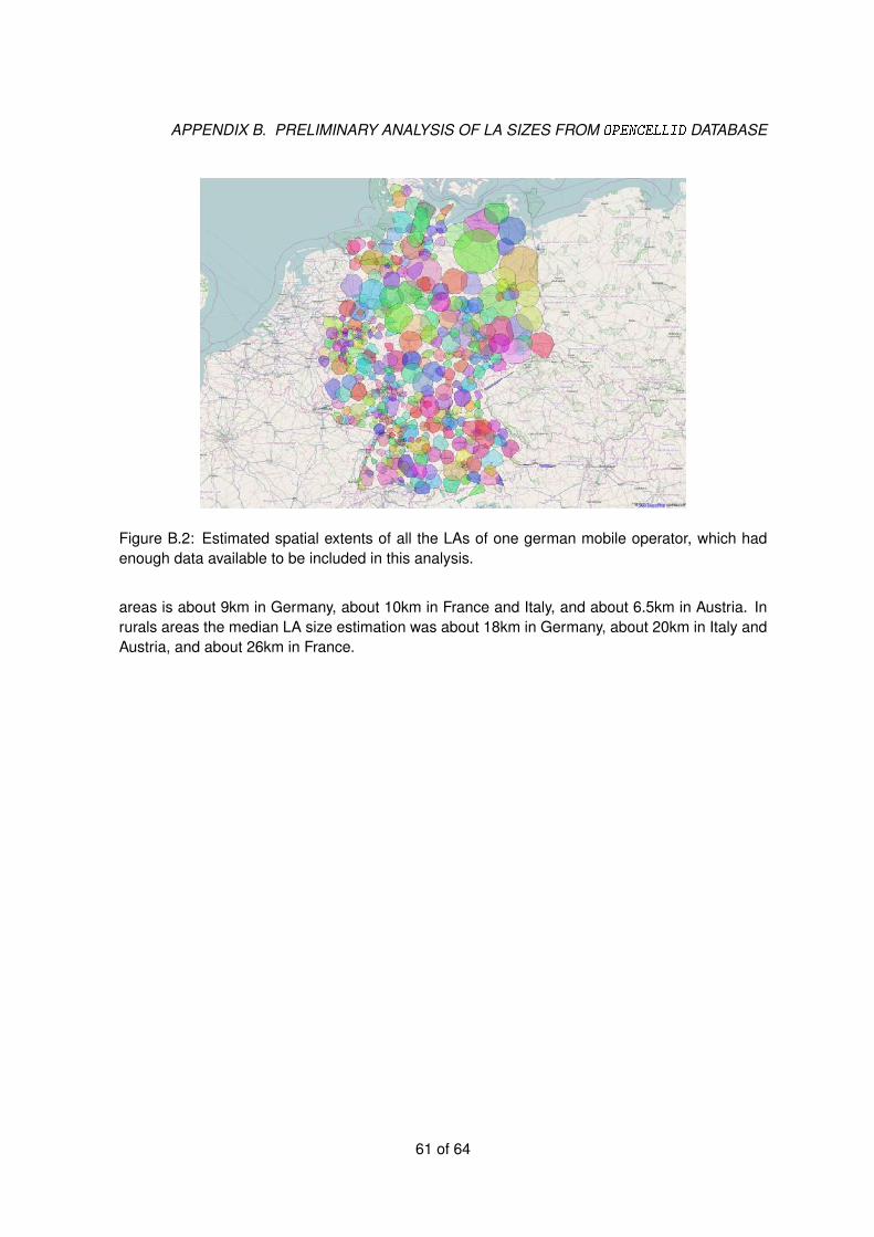
APPENDIX B. PRELIMINARY ANALYSIS OF LA SIZES FROM OPENCELLID DATABASE
Figure B.2: Estimated spatial extents of all the LAs of one german mobile operator, which hadenough data available to be included in this analysis.
areas is about 9km in Germany, about 10km in France and Italy, and about 6.5km in Austria. Inrurals areas the median LA size estimation was about 18km in Germany, about 20km in Italy andAustria, and about 26km in France.
61 of 64

APPENDIX B. PRELIMINARY ANALYSIS OF LA SIZES FROM OPENCELLID DATABASE
Figure B.3: Densely populated areas used for the analysis of Location Area sizes in urban andrural areas (data taken from [1].
0 10 20 30 40 50 60 70 80 90 1000
0.1
0.2
0.3
0.4
0.5
0.6
0.7
0.8
0.9
1
km
F
Germany
urban areasrural areas
0 10 20 30 40 50 60 70 80 90 1000
0.1
0.2
0.3
0.4
0.5
0.6
0.7
0.8
0.9
1
km
F
France
urban areasrural areas
0 10 20 30 40 50 60 70 80 90 1000
0.1
0.2
0.3
0.4
0.5
0.6
0.7
0.8
0.9
1
km
F
Italy
urban areasrural areas
0 10 20 30 40 50 60 70 80 90 1000
0.1
0.2
0.3
0.4
0.5
0.6
0.7
0.8
0.9
1
km
F
Austria
urban areasrural areas
Figure B.4: Emprical CDF of Location Area sizes in Germany, France, Italy, and Austria.
62 of 64

APPENDIX B. PRELIMINARY ANALYSIS OF LA SIZES FROM OPENCELLID DATABASE
List of Acronyms
APN Access Point NameBSC Base Station ControllerBTS Base Transceiver StationCDR Call Detail RecordCGI Cell Global IdentifierCN Core NetworkCS Circuit SwitchedGGSN Gateway GPRS Support NodeHLR Home Location RegisterIMEI International Mobile Equipment IdentityIMSI International Mobile Subscriber IdentityLA Location AreaLAC Location Area CodeLAI Location Area IdentityLAU Location Area UpdateMCC Mobile Country CodeMCD Map/Counter Dataset (*)MNC Mobile Network CodeMNO Mobile Network OperatorMS Mobile StationMSC Mobile Switching CenterPLMN Public Land Mobile NetworkPS Packet SwitchedRAN Radio Access NetworkRA Routing AreaRAC Routing Area CodeRAI Routing Area IdentityRNC Radio Network ControllerSIM Subscriber Identity ModuleSGSN Serving GPRS Support NodeSMS Short Message ServiceTA Tracking AreaTAC Type Allocation CodeT-IMSI Temporary IMSIVLR Visiting Location Register
(*) This acronym was defined in this document and is not part of the standard 3GPP terminology.
63 of 64

Bibliography
[1] Natural earth data. www.naturalearthdata.com. Accessed: 2015-01-10.
[2] OpenCellID. http://opencellid.org. Accessed: 2014-10-20.
[3] ETSI TS 132 215. Charging data description for the packet switched (ps) do-main. In http: // www. etsi. org/ deliver/ etsi_ ts/ 132200_ 132299/ 132215/ 05.
09. 00_ 60/ ts_ 132215v050900p. pdf .
[4] F. Aurenhammer. Voronoi diagrams — a survey of a fundamental geometric data structure.ACM Computing Surveys, 23(3), 1991.
[5] Center for Spatial Information Science — Univ. of Tokyo. A study on urban mobility anddynamic population estimation by using aggregate mobile phone sources. http://www.
csis.u-tokyo.ac.jp/dp/115.pdf.
[6] K. L. Clarkson, D. Eppstein, G. L. Miller, C. Sturtivant, and S.-H. Teng. Approximating centerpoints with iterative radon points. Int. J. Comput. Geom. Appl., 357(06), 1996.
[7] H. Edelsbrunner. Algorithms in Combinatorial Geometry. Springer Verlag, 1987.
[8] P. D. et al. Dynamic population mapping using mobile phone data. PNAS, 111(45), Novem-ber 2014.
[9] F. Ricciato. Traffic monitoring and analysis for the optimization of a 3g network. IEEE Wire-less Communications — Special Issue on 3G/4G/WLAN/WMAN Planning, 13(6), December2006.
[10] F. Ricciato et al. Traffic monitoring and analysis in 3G networks: lessons learned from theMETAWIN project. Elektrotechnik & Informationstechnik, 123/7/8, 2006.
[11] J. Friedman. On bias, variance, 0/1-loss, and the curse-of-dimensionality. Data Mining andKnowledge Discovery, 1(1), 1997.
[12] INSPIRE Thematic Working Group Coordinate Reference Systems and GeographicalGrid Systems. D2.8.I.2 Data Specification on Geographical Grid Systems — Tech-nical Guidelines. http://inspire.ec.europa.eu/documents/Data_Specifications/
INSPIRE_DataSpecification_GG_v3.1.pdf. Accessed: 2015-03-27.
[13] A. Janecek, D. Valerio, K. A. Hummel, F. Ricciato, and H. Hlavacs. The cellular network asa sensor: From mobile phone data to real-time road traffic monitoring. IEEE Transaction onIntelligent Transportation Systems, 2015.
64

BIBLIOGRAPHY
[14] F. Pantisano and M. Craglia. Mobile network operator data to support urban planning andmanagement. JRC working document, 2015.
[15] S. Tartarelli, N. d’Heureuse, and S. Niccolini. Lessons learned on the usage of call logsfor security and management in ip telephony. IEEE Communications Magazine, 48(12),December 2010.
65 of 64

Europe Direct is a service to help you find answers to your questions about the European Union
Freephone number (*): 00 800 6 7 8 9 10 11
(*) Certain mobile telephone operators do not allow access to 00 800 numbers or these calls may be billed.
A great deal of additional information on the European Union is available on the Internet.
It can be accessed through the Europa server http://europa.eu.
How to obtain EU publications
Our publications are available from EU Bookshop (http://bookshop.europa.eu),
where you can place an order with the sales agent of your choice.
The Publications Office has a worldwide network of sales agents.
You can obtain their contact details by sending a fax to (352) 29 29-42758.
European Commission
EUR 27361 EN - Joint Research Centre – Institute for Environment and Sustainability
Title: Estimating population density distribution from network-based mobile phone data
Authors: Fabio Ricciato, Peter Widhalm, Massimo Craglia and Francesco Pantisano
Luxembourg: Publications Office of the European Union
2015 – 65pp. – 21.0 x 29.7 cm
EUR – Scientific and Technical Research series – IISSN 1831-9424 (online)
ISSN 978-92-79-50193-7 (PDF)
doi:10.2788/162414

JRC Mission As the Commission’s in-house science service, the Joint Research Centre’s mission is to provide EU policies with independent, evidence-based scientific and technical support throughout the whole policy cycle. Working in close cooperation with policy Directorates-General, the JRC addresses key societal challenges while stimulating innovation through developing new methods, tools and standards, and sharing its know-how with the Member States, the scientific community and international partners.
Serving society Stimulating innovation Supporting legislation
LB
-NA
-27
36
1-E
N-N
doi:10.2788/162414
ISBN 978-92-79-50193-7


