Estimating Price Elasticities in Di ff erentiated Product Demand Models with Endogenous Characteristics Daniel A. Ackerberg ∗ UCLA Gregory S. Crawford University of Arizona March 27, 2009 Preliminary and Incomplete - Please do not distribute Abstract Empirical models of differentiated product demand have typically allowed price to be endogenous, but proceed under the assumption that observed product characteristics are exogenous, i.e. uncorrelated with unobserved components of demand. This paper shows that such an assumption may not be necessary to obtain consistent estimates of price elasticities. We show that whether this is the case depends on properties of the instrument or instruments used for price. Since these properties are testable, this result has interesting implications on an applied researcher’s choice of price instruments. In the case where one cannot find an instrument that satisfies these properties, one can often bound the potential bias in estimated price elasticities due to endogenous product characteristics. Our ideas also lead to interesting thoughts about what sorts of variables would ideally like to have as price instruments. Lastly, we apply these ideas to data on demand for cable television, obtaining estimates of price elasticities that are in fact robust to endogenous product characteristics. ∗ Thanks to Jin Hahn and Joris Pinkse for comments and helpful discussion. All errors are our own. 1
Transcript
Estimating Price Elasticities in Differentiated Product
Demand Models with Endogenous Characteristics
Daniel A. Ackerberg∗
UCLA
Gregory S. Crawford
University of Arizona
March 27, 2009Preliminary and Incomplete - Please do not distribute
Abstract
Empirical models of differentiated product demand have typically allowed price to be
endogenous, but proceed under the assumption that observed product characteristics are
exogenous, i.e. uncorrelated with unobserved components of demand. This paper shows that
such an assumption may not be necessary to obtain consistent estimates of price elasticities.
We show that whether this is the case depends on properties of the instrument or instruments
used for price. Since these properties are testable, this result has interesting implications
on an applied researcher’s choice of price instruments. In the case where one cannot
find an instrument that satisfies these properties, one can often bound the potential bias
in estimated price elasticities due to endogenous product characteristics. Our ideas also
lead to interesting thoughts about what sorts of variables would ideally like to have as price
instruments. Lastly, we apply these ideas to data on demand for cable television, obtaining
estimates of price elasticities that are in fact robust to endogenous product characteristics.
∗Thanks to Jin Hahn and Joris Pinkse for comments and helpful discussion. All errors are our own.
1
1 Introduction
The recent literature in empirical IO has devoted significant effort to developing methodology for
estimating demand systems in differentiated product markets. This is understandable since 1)
many, if not most, markets are characterized by product differentiation, and 2) demand systems
are a crucial component of many interesting IO questions. For example, an analysis of the price
effects of mergers will depend on estimates of own and cross-price elasticities, which will typically
come from an estimated demand system. An estimated demand system is also crucial for, e.g.,
measuring elasticities w.r.t. product characteristics, computing the welfare effects of new products
or price changes, and creating optimal price indices. They can also be important indirect inputs
in answering many other interesting IO questions. The general idea here is that if one is going to
address general IO issues, one typically needs to have the demand system right.
Starting with Bresnahan (1987) and Berry, Levinsohn, and Pakes (1995, henceforth BLP), an
important contribution of this methodology has been to base these demand systems on character-
istics of the various products. This reduces the dimensionality of the system from the number of
products available on the market (which can be very large, e.g. automobiles or computers) to the
dimension of product characteristic space, making estimation feasible. Another key issue that has
been addressed is that of price endogeneity. Given prices are choice variables of firms, it is likely
that they will respond to components of demand that are unobserved to the econometrician, cre-
ating an endogeneity problem. Estimation has typically proceeded by trying to find appropriate
"instruments" for price in order to solve this endogeneity problem.
In contrast, both the developers and appliers of this methodology have admittedly ignored
potential endogeneity of product characteristics. In other words, practitioners have relied on the
assumption that product characteristics are exogenous. Just like price, product characteristics are
typically choice variables of firms, and as such one might worry that they are actually correlated
with unobserved components of demand.
So why have existing studies relied on the assumption that product characteristics are ex-
ogenous? One reason is that it is likely in many intances that product characteristics are less
endogenous than price. The idea here is that since price is often a more flexible decision than
are product characteristics, it might be expected to be more correlated with unobserved demand
components. On the other hand, it would certainly be preferable to allow for endogenous prod-
uct characteristics as well. A second reason is that currently there are no particularly attractive
alternatives. One possibility is to instrument for product characteristics as well as price, but this
would require finding instruments for each product characteristics. It is already hard enough
finding credible instruments for price. In addition, when one allows for the possibility of unob-
served product characteristics, it is hard to imagine being able to find such instrumental variables.
They would need to be correlated with observed product characteristics, but uncorrelated with
unobserved product characteristics. It is unclear what variables would satisfy such a requirement.
2
Another possibility, suggested by BLP (and applied recently in Sweeting (2008) and Fan (2009)),
involves setting up moments in terms of innovations in demand unobservables rather than the
demand unobservables themselves. This, when accompanied by an assumption on what firms’
information sets contain at the time when product characteristics are decided, can provide consis-
tent estimates even when product characteristics are endogenous. BLP admit that this solution,
which in practice involves psuedo-differencing the data, can be demanding on the data and we
have yet to see it applied.
Lastly, one could imagine actually modelling firms’ choices of product characteristics. Crawford
and Shum (2006) take this approach. While this might be the most appealing approach to the
problem conceptually, it ends up being quite complicated in practice. As such, Crawford and Shum
are forced to restrict attention to monopoly markets (although multiproduct) where there is only
a one dimensional product characteristic. Their approach would be much harder if not impossible
to apply to either oligopoly markets or markets with multidimensional product characteristics.
Pioner (2008) studies non-parametric identification in a similar model.
Our paper takes a different, simpler, approach to the problem of endogenous product charac-
teristics. We start with the observation that one does not always need to estimate causal effects of
changing product characteristics - for many questions, e.g. most short-run antitrust questions, one
is primarily interested in own and cross price elasticities. Given this, we ask the following ques-
tion: under what conditions will we get consistent estimates of price elasticities, even if product
characteristics are endogenous?
Some simple econometric derivations show that under particular assumptions on our price in-
struments, standard estimation procedures (e.g. BLP) do in fact return consistent estimates of
price elasticities, even if product characteristics are endogenous. These assumptions involve cor-
relations between the instruments and the endogenous product characteristics, and perhaps most
important, are testable. As a result, one can 1) test if our estimates are consistent even if prod-
uct characteristics are endogenous, and 2) if not, perhaps appropriately choose price instruments
to generate estimates that are robust to endogenous product characteristics. The analysis also
sheds light on what types of data generating processes would generate instruments that satisfy
this condition. In some cases where we cannot obtain consistent estimates of price elasticities, we
can bound the bias in these estimates.
We end by illustrating our methodology using a dataset on demand for cable television. The
data includes information from almost 5000 cable systems across the US. Our two key explanatory
variables are price and the product characteristic "number of cable networks" offered. We have
a number of potential price instruments, and we are able to test the above conditions for each of
the various instruments. One of these instruments satisties this condition, and thus by using this
instrument we are able to consistently estimate price elasticities allowing for endogenous product
characteristics. Interestingly, this instrument also gives more reasonable price elasticities than the
others.
3
2 Econometric Preliminaries
We start by discussing some relatively simple econometric results that are relevant for our treat-
ment of endogenous product characteristics. These results all concern instrumental variables
estimation of casual effects in the presence of covariates. A key difference from the standard
treatment of instrumental variables is that we will consider a situation where one is not interested
in estimating the casual effects of the covariates (on the dependent variable). This allows us
to use identification conditions that are slightly different than the standard IV conditions. We
later argue that these alternative identification conditions are particularly useful in a situation
where product characteristics are endogenous. Another interesting attribute of these alternative
identification conditions is that they are partially testable. We start by showing these ideas in
a linear situation, and then generalize the ideas to the non-parametric model of Chernozhukov,
Imbens, and Newey (2006).
2.1 Linear Model
Consider a linear model of the form
(1) yi = β1xi + β2pi + i
β1 and β2 respectively measure the causal effects of observables xi and pi on yi. i represents
unobservables that also affect yi. Looking ahead to our application, one might interpret (1) as
the demand curve for a product whose characteristics and price vary across markets - pi is the
price in market i, xi is an L-vector of the product’s characteristics in market i, and yi is quantity
demanded. i are unobservables that could represent either characteristics of the product that are
not observed by the econometrician or demand shocks in market i.
Throughout, we will assume that pi is potentially correlated with i, i.e. that it is endogenous.
We will also consider the possibility that xi is endogenous. As mentioned in the introduction and
above, a key distinction between xi and pi is that we assume that we are primarily interested in
estimating the causal effect of pi on yi. In contrast we are less interested or not interested in the
causal effects of xi on yi. We assume that we observe zi, a potential instrument for pi. In the
demand context, one can think of zi as a cost shifter. In contrast, we assume we do not have
outside instruments for the covariates xi. WLOG, all variables are assumed mean-zero.
Consider IV estimation of (1) using (xi, zi) as instruments for (xi, pi). Aside from regularity
and rank conditions, the typical assumptions made to ensure identification of the causal effect β2are
Assumption L1: E [ izi] = 0, E [ ixi] = 0
Note that for simplicity we are considering the necessity for the instrument zi to be correlated
4
with pi (conditional on xi) as a "rank" condition. This will be implicitly assumed throughout.
There are two compoments of Assumption (L1). The first states that zi is a valid instrument
for pi, i.e. it is uncorrelated with the residual. As is well known, without outside instruments,
E [ ixi] = 0 is also generally necessary for identification of β2. Even if E [ izi] = 0, any correlation
between i and xi will generally render IV estimates of β2 inconsistent.This "transmitted bias" in
analagous to that when one uses OLS when one regressor is exogenous and another is endogenous
- in that case, OLS generally produces inconsistent estimates of both coefficients.
Now consider the following alternative set of assumptions
Assumption L2: E [ izi] = 0, E [zixi] = 0
Note the distinction between (L1) and (L2) arises in the second component - while (L1) requires
xi to be uncorrelated with i, (L2) requires xi to be uncorrelated with zi.
One can easily show that (again assuming regularity and rank conditions hold) that (L2)
ensures identification of the causal effect β2. To see this, decompose i into its linear projection
on xi and a residual, i.e.
i = λxi + eiand consider the transformed model
(2) yi = eβ1xi + β2pi + eiwhere eβ1 = β1 + λ.
By construction,
(3) E [eixi] = 0In addition,
(4) E [eizi] = E [( i − λxi)zi] = E [ izi]− λE [xizi] = 0
by (L2). Together, (3), (4) imply that the transformed model (2) satisfies (L1). Hence, applying
IV to this model produces consistent estimates of eβ1 and β2. While eβ1 = β1 + λ is not the causal
effect of xi on yi, β2 is the causal effect of pi on yi, so IV under (L2) consistently estimates the
parameter we are interested in.
There are a couple of intuitive ways to think about this result. First, for some intuition behind
why this works, note that under (L2), we could simply ignore xi - lumping it in with the error
term. This results in the model
yi = β2pi + (β1xi + i)
5
Since zi is uncorrelated with both xi and i, it is uncorrelated with the composite error term
(β1xi+ i). Hence, IV consistently estimates β2. Of course, one would never do this in practice, as
the resulting estimator would be inefficient relative to the one including xi as a covariate. A second
source of intuition behind the result is that because xi and zi are uncorrelated, the "transmitted
bias" on β2 described above disappears. This is again analagous to the more well-known OLS
result - suppose that pi is exogeous and xi is endogenous - in this case OLS can consistently
estimate the causal effect of pi when pi and xi are uncorrelated. However, in a moment we argue
that this is a much more powerful result in an IV setting.
In summary, we can obtain consistent estimates of the causal effect of pi on yi even if other
covariates xi are endogenous and we have no outside instruments for them. We feel that this
is an underappreciated result for a number of reasons. First, it is always preferable to have
more possible identifying assumptions - in some cases, one simply might be more willing to make
assumption (L2) than assumption (L1). Second, an important distinction between (L1) and (L2)
is that while (L1) is not a directly testable set of assumptions1, part of (L2) is directly testable.
Specifically, one can fairly easily check whether E [zixi] = 0 in one’s dataset. This can then
allow one to relax the assumption that E [ ixi] = 0. Thirdly, taking somewhat of a Bayesian
perspective, we feel that in some cases, verifying that E [zixi] = 0 may make us more confident
in the untestable assumption that E [ izi] = 0. The basic idea here is that if i is analagous to
xi (except for the fact that i is unobserved to the econometrician), e.g. xi are observed product
characteristics, i are unobserved (to the econometrician) product characteristics, a finding that
E [zixi] 6= 0 might make one worried that E [ izi] = 0. In our empirical model we investigate thisidea further.
Lastly, compare this result to the OLS result described above where pi is exogeous and xi is
endogenous. In the OLS case, pi and xi will either be correlated or not - there is not much one
can do to estimate the causal effect of pi if they are correlated. On the other hand, in the IV case,
there is the possibility that one has multiple instruments for pi. In this case, one can explicitly
look for potential instruments that satisfy E [zixi] = 0. If one can find such an instrument
(or instruments), we have shown that one can estimate β2 consistently even with an endogenous
xi. This result is therefore important for the instrument selection issue when one is concerned
about an endogenous xi. More specifically, one can look for instruments that satisfy this property.
Later, this ends up being a key goal of our empirical model. Even if one is reasonably comfortable
assuming that xi is exogenous, it seems to us that examining E [zixi] might be useful to examine
possible "robustness" to violations of this assumption.
1It could be indirectly testable in the case where one has overidentifying restrictions, but those tests rely onauxiliary assumptions.
6
2.2 Non-linear Models
We next examine if this result holds up as we move to more flexible, non-parametric models.
As an example, we consider the non-parametric IV model of Chernozhukov, Imbens, and Newey
(2006) (CIN), i.e.
(5) yi = g(xi, pi, i)
where xi and pi are defined as above. Two important restrictions of the CIN model are that i
is a scalar unobservable and that g is strictly monotonic in i. While this does allow for some
forms of unobservable heterogeneous treatment effects (where the effect of pi on yi depends on
unobservables) it is not completely flexible in this dimension. On the other hand, the model
is completely flexible in allowing heterogenous treatment effects that depend on the observed
covariates xi. CIN normalize the distribution of i to be U(0, 1) - this is WLOG because of the
non-parametric treatment of g - intuitively, an appropriate g can turn the uniform random variable
into whatever distribution one wants.
The analogue of causal effects in the CIN model are "quantile treatment effects". Specifically,
g(x0i, p0i, qτ)− g(xi, pi, qτ)
is the causal effect on yi from moving from (xi, pi) to (x0i, p0i), evaluated at the τth quantile of the
i distribution. Given the above normalization of i to be U(0, 1), this is also the causal effect of
moving from (xi, pi) to (x0i, p0i) conditional on i = qτ . As in the above linear model, we assume
that we are only interested in estimating the causal effects of changing pi. In other words, the
"quantile treatment effects" we are interested in are all given a fixed xi (i.e. involve x0i = xi).
Again ignoring regularity and rank conditions, the key identification assumption of CIN is
Assumption N1: (xi, zi) are jointly independent of i
This independence condition is considerably stronger than the zero correlation conditions in the
linear model, but that is what is typically required for non-parametric identification of these sorts
of models. More importantly for our purposes, while this assumption allows arbitrary correlation
between pi and i, it assumes that xi is exogenous.
Our question is whether, as was done in the linear model, we can replace the assumption that
i is independent of xi with an alternative assumption relying more on assumptions regarding the
relationship between xi and zi. It turns out we can. Consider
Assumption N2: (xi, i) are jointly independent of zi
To consider estimation under (N2), we first show that (N2) implies that iand ziare indepen-
7
dent conditional on xi. To prove this, note that
p(zi, i|xi) =p(zi, i, xi)
p(xi)
=p(zi)p( i, xi)
p(xi)
= p(zi)p( i|xi)= p(zi|xi)p( i|xi)
where the second and last equalities follow from (N2).
What is the meaning of this result? (N2) states directly that our instrument is valid (in the
sense of being independent of i) in the entire population. This simple implication of (N2)
says that our instruments continue to be valid even after conditioning on xi. That is to say,
conditioning on xi does not generate correlations between zi and i. The importance of this result
is quite intuitive - it says we can simply condition on xi to avoid the problem of xi being correlated
with i - doing this conditioning does not destroy the properties of our instrument.
To formally do this conditioning, assume that xi has a discrete support to avoid technical
issues. Pulling the xi dependence into the g function, we get
(6) yi = gxi(pi, i)
Think about estimating this transformed model separately for each possible value in the support of
xi. As just shown, conditional on being at each of these support points, i and zi are independent.
Of course, because of the correlation between i and xi, the distribution of i will vary across these
support points. At each support point, renormalize the distribution of i to be U(0, 1) - this only
involves changing gi. This transformed model now satisfies (N1) - hence, the CIN result suggests
that we can estimate quantile treatment effects of this transformed model.
Importantly, because we have completely conditioned on xi, our quantile treatment effects are
conditioned completely on xi. That is,
gxi(p0i, qτ)− gxi(pi, qτ)
is the causal effect on yi from moving from (pi) to (p0i), evaluated at the τth quantile of the i
distribution conditional on xi. These are different than the quantile treatment effects of the
untransformed model (which would estimate the causal effect on yi from moving from (pi) to (p0i),
evaluated at the τth quantile of the unconditional i distribution), but fine for many empirical
purposes, particularly in empirical Industrial Organization .
Summarizing, we have shown that as in the linear model, we do not have to necessarily assume
that the covariates xi are exogenous to estimate the causal effect of pi on yi. We can instead look
8
for instruments for pi that appear to be independent of the covariates xi. Note that assumption
(N2) is not quite as testable as in the linear case. Not only does zi have to be independent of each
of xi and i individually, but zi has do be independent of the entire joint distribution of (xi, i).
The only part of this that is directly testable is that zi is independent of xi. However, this still
should be a useful test. In addition, again appealing to a pseudo Bayesian perspective, finding
evidence that zi is independent of xi may be supportive of the assumption that zi is independent
of i and the joint distribution (xi, i).
Before continuing, note that there is a third possible identifying assumption that one could
also use to identify the above model. One could directly make the assumption that i and zi are
independent conditional on xi, i.e.
Assumption N3: (zi, i) are independent conditional on xi
Identification of conditional quantile treatment effects under this assumption follows directly
from the above. Note that while (N2) implies (N3), the reverse is not so. We think there are
at least two important examples when this is the case. First, note that under (N3), there can
actually be correlation not only between zi and xi, but also between xi and i. Suppose, for
example
zi = f1(xi) + η1i
i = f2(xi) + η2i
If η1i and η2i are independent (conditional on xi), then (N3) will hold, even though both zi and i
are correlated with xi. Given the structure of these two equations, this type of assumption might
be appropriate when xi’s are can be thought of as being determined outside the economic model
under consideration.
As a second example, suppose that zi satisfies (N2), i.e. (xi, i) are jointly independent of zi.
But suppose that the econometrician does not directly observe the instrument zi. Suppose instead
that what is observed is some function of zi and xi, i.e.:
z∗i = h(zi, xi)
In this case, while the observed instrument z∗i certainly does not satisfy (N2), it does satisfy (N3).
Hence, the causal effect of the endogenous pi will be identified. Note that this would also be the
case if other random variables ηi that are independent of xi and i also entered the above equation,
e.g.
z∗i = h(zi, xi, ηi)
9
2.3 Combining Identification Assumptions
Note that one can use different types of the above identification assumptions for different covariates.
For example, suppose we expand our demand model to the following
(7) yi = g(mi, xi, pi, i)
where now bothmi and xi are covariates. Again, suppose that we are only interested in estimating
the causal effect of pi on yi. Consider the following assumption
Assumption N4: (xi, i) are jointly independent of zi, conditional on mi
Assumption (N4) essentially combines assumption (N2) on the xi covariates and assumption
(N3) on the mi covariates. To verify that we can identify conditional (on mi and xi) quantile
treatment effects in this model, we just need to show that (N4) implies that (zi, i) are independent
conditional on xi and mi, i.e.
p(zi, i|xi,mi) =p(zi, i, xi|mi)
p(xi|mi)
=p(zi|mi)p( i, xi|mi)
p(xi|mi)
= p(zi|mi)p( i|xi,mi)
= p(zi|xi,mi)p( i|xi,mi)
Given this result, it follows from the above (treating xi = (xi,mi)) that we can identify the
conditional quantile treatment effects.
Why might we want to treat our covariates asymetrically? Recall our demand example.
Suppose that mi are market characteristics (e.g. the distribution of income, population density,
etc.) and that xi and i are respectively, observed and unobserved (to the econometrician) product
characteristics. Recall that pi is price, zi is an instrument for price, and yi is demand for the
product. If zi, are e.g. input price shocks, it seems presumptous to assume that they are
independent of general market characteristics. However, it does seem plausible that, conditional
on market conditions, variation in zi might be independent of product characteristics xi and i.
3 Bounding Bias
Moving back to the linear case, the above derivations consider the situation where the instrument
is uncorrelated with the endogenous product characteristics. But what if one is unable to find
10
such an instrument? It turns out that in these cases, one can often use the observed correlation
between the instrument and the endogenous product characteristics to bound the possible bias on
the price coefficient. For related ideas, see Nevo and Rosen (2006). Among other things, this can
be used to choose between possible instruments.
In this section, we currently consider only two explanatory variables, although we extend this
below. We also start by just examining the OLS case - i.e. where one explanatory variable is
endogenous, and the question is how much bias is imparted on the other coefficient. Later we
move to the IV case we have been discussing above.
Consider the following model:
yi = β1x1i + β2x2i + i
where all variables have been demeaned. Suppose that x1 is potentially correlated with the
residual , but x2 is uncorrelated with . Our primary concern is to estimate the parameter β2.
Consider the OLS estimator formed by regressing y on x1 and x2.
βOLS = (X0X)−1X 0y
where
X =
⎡⎢⎢⎢⎣x11 x21
. .
. .
x1N x2N
⎤⎥⎥⎥⎦ y =
⎡⎢⎢⎢⎣y1
.
.
yN
⎤⎥⎥⎥⎦Substituting in, we get:
βOLS = (X 0X)−1X 0y
= (X 0X)−1X 0(Xβ + )
= β + (X 0X)−1X 0
The second term is a bias term. Looking at the plim of this bias term in more detail, we have:
p lim(X 0X)−1X 0 =
"p lim 1
N
Pi x21i p lim 1
N
Pi x1ix2i
p lim 1N
Pi x1ix2i p lim 1
N
Pi x22i
#−1 "p lim 1
N
Pi x1i i
0
#
The zero in the second element of X 0 follows because of the assumption that x2 is uncorrelated
with . WLOG, normalize the variance of each of x1i and x2i to unity. This generates a bias
term of
(X 0X)−1X 0 =
"1 Cov(x1i, x2i)
Cov(x1i, x2i) 1
#−1 "Cov(x1i, i)
0
#
11
Inverting the matrix manually generates a bias vector of:
We are only concerned with the second term in this bias vector, i.e.
bias =−Cov(x1i, x2i)1− Cov(x1i, x2i)2
Cov(x1i, i)
The absolute value of this bias is
abs(bias) =abs(Cov(x1i, x2i))
1− Cov(x1i, x2i)2abs(Cov(x1i, i))
First note that this bias term is increasing in the absolute value of Cov(x1i, x2i) over its feasible
range (−1 < Cov(x1i, x2i) < 1). This means that given any level of correlation between x1i and
i, lower (absolute) values of Cov(x1i, x2i) indicate lower values of bias.
Next, note that Cov(x1i, x2i) is observed by the econometrician. Given this, our question is
whether we can bound this bias. Unfortunately, Cov(x1i, i) is not observed by the econometrician,
and can in general can take any value from -∞ to∞ (as long as V ar( i) is set high enough). Hence,
we need to make some additional assumptions in order to bound this bias term. There are a couple
of ways to proceed.
First, one could make a direct assumption on the possible range of Cov(x1i, i). However,
this seems like a strange term to be making a-priori assumptions on. Alternatively, note that the
covariance of two variables is bounded by the product of their two variances, i.e.
abs(Cov(x1i, i)) < SD(x1i)SD( i)
< SD( i)
This implies that that:
abs(bias) <abs(Cov(x1i, x2i))
1− Cov(x1i, x2i)2SD( i)
This bound can potentially be pretty tight. Suppose for example that x1i, x2i, and i all contribute
"equally" (in a causal sense) to yi. This would be the case if we set β1 = 1, β2 = 1, and SD( i) = 1.
Then if, for example, Cov(x1i, x2i) = 0.2, the maximal bias is 0.2, or 20% - this maximum occurs
when x1i and i are perfectly correlated.
It turns out that one can actually shrink these bounds a bit more. The reason is that if x1i and
x2i are correlated and x2i and i are uncorrelated, then x1i and i cannot be perfectly correlated.
However, this does not increase the bound by much when Cov(x1i, x2i) is small, so we ignore this
approach for now.
12
Of course, the above assumption that SD( i) <= 1 is one that could certainly seem arbitrary.
Is there any natural upper bound for SD( i)? One somewhat natural bound might be the standard
deviation of the dependent variable SD(yi). It is not necessarily the case that SD( i) is less than
SD(yi). However, there is a more primitive assumption that generates this result - that i is
positively correlated with β1x1i + β2x2i. This condition can also hold if i is negatively correlated
with β1x1i + β2x2i, but it cannot be too negatively correlated. Formally,
V ar(yi) = V ar(βxi) + V ar( i) + 2Cov(βxi, i)
Therefore:
V ar(yi) > V ar( i)⇔ V ar(βxi) + 2Cov(βxi, i) > 0
⇔ V ar(βxi) + 2Corr(βxi, i)SD(βxi)SD( i) > 0
This clearly indicates that if Corr(βxi, i)̇ > 0, then SD( i) < SD(yi). But even if Corr(βxi, i)̇ <
0, then the condition will still hold unless Corr(βxi, i) is very negative and SD( i) is reasonably
high. For example, note that if we assume that the observed characteristic are "twice as impor-
tant" as unobserved characteristics (in the sense that SD(βxi) > 2SD( i)), then the condition
must hold, even if Corr(βxi, i) = −1.A couple of more notes - in the BLP context, at least the price component of βxi will be
negatively correlated with i. This is slightly problematic for the potential argument that
Corr(βxi, i)̇ > 0 (but not for the potential argument that SD(βxi) > 2SD( i)). Another way
motivate this condition is using a hypothetical thought experiment. Suppose, we took a dataset
(i.e. observed xi’s and yi’s) and forced all xi’s to their means. The question is what is the variance
of the new yi’s. If one is willing to assume that the new yi’s are not as varied as the original yi’s
then SD( i) must be < SD(yi).
4 Application to the Discrete Choice Demand Literature
The above results can be straightforwardly applied to the literature on estimating demand systems
in differentiated product markets. This literature often works with data across markets that is
aggregated to the product level. For example, for each product j in market t, one typically
observes pjt (prices), Xjt (a vector of product characteristics), and sjt (product j’s market share
in market t)
The logit-based utility model generates an estimating equation of the following form (see Berry
(1994))
ln
µsjts0t
¶= Xjtβ − αpjt + ξjt
13
where ξjt is the econometric error (these are typically interpreted as either unobserved product
characteristics or shocks to demand). Estimation of these models is typically done using IV/2SLS
using instruments for pjt. In other words, estimation proceeds allowing pjt to be endogenous and
correlated with ξjt, but under the assumption that product characteristics are exogenous, i.e.
uncorrelated with ξjt. Instruments zjt come from various sources, including, e.g., traditional
cost shifters, characteristics of competing products in the market (see Bresnahan (1987) and BLP
(1995) for motivation), and prices of the same product in other markets (see Hausman (1997) and
Nevo (2001) for motivation).
Under the maintained assumption that the instruments are uncorrelated with ξjt, one will
obtain consistent estimates of β and α as long as the product characteristics Xjt are uncorrelated
with ξjt. However, if these product characteristics are correlated with ξjt, then estimates of both
β and α will be biased - β suffers a direct bias due to the endogeneity of Xjt, and α generally
suffers a transmitted bias. The derivations above, however, show that in the case where the
instrument zjt is uncorrelated with Xjt, there is no transmitted bias. In this case, α will be
estimated consistently with the IV/2SLS estimator (though the estimate of β will still be biased).
There are at least a couple of approaches to using this result. First, one can simply look for
instruments that satisfy this condition. Since the condition can be directly tested, this is relatively
straightforward. Second, one can use theory to think about what choices of instruments might
satisfy this condition. One interesting example of this uses cost shifters as instruments and is
based on timing assumptions. Suppose that product characteristics Xjt are chosen before price
pjt. This seems like a natural assumption for many products where prices can be varied quite
rapidly, but product characteristics need to be designed and planned in advance. In such a
situation, one would want to use cost shocks that are realized by firms between the points in time
. Such instruments would be uncorrelated with Xjt but likely correlated with pjt. A specific
example would be a situation in which there are futures markets for the price of an input. In this
case, one would want to use the difference between the realized input price at the time when pjt
is set, and the expected future value of that input price at the time when Xjt was set. This by
construction should be uncorrelated with Xjt . Of course, this correlation can be tested, which
would be an implicit test of the timing assumption used to generate the condition.
One important additional point is that under these conditions, we have shown that α can be
consistently estimated. α measures the marginal effect of price on utility. However, in many
cases, a key goal of IO researchers is to estimate own and cross price elasticities/derivatives, which
potentially depend on all parts of the model, i.e. both β and α. It is not directly obvious that
these elasticities/derivatives can be estimated, since we cannot consistently estimate β. However,
14
one can easily show that in this model, own and cross price derivatives can be written as:
∂sjt∂pjt
= −αsjt(1− sjt)
∂sjt∂pkt
= αsjtskt
This indicates that price derivatives (and elasticities) can be written only as a function of the data
and the estimated α - not of the estimated β. Hence these price derivatives and elasticities can be
estimated consistently. Of course, note that we cannot recover elasticities w.r.t. characteristics,
since those will obviously depend on β.
This result also applies to more flexible differentiated product demand models. The estimating
equation in the nested logit model can be expressed as:
ln
µsjts0t
¶= Xjtβ − αpjt + σ ln(sjt|g) + ξjt
where sjt|g measures product j’s within-group (nest) market share, and σ is a parameter measuring
how substitution patterns differ within and across nests. Since sjt|g is by construction endogenous
in these models, one needs at least two instruments to deal with the endogenous pjt and sj|g. Our
results above indicate that if these instruments are uncorrelated withXjt, then IV/2SLS estimation
of the above equation produces consistent estimates of α and σ, even if Xjt is endogenous. One
can easily show that in these models, price derivatives can be written as:
∂sjt∂pjt
= −αsjt(1
1− σ− σ
1− σsjt|g − sjt)
∂sjt∂pkt
=
(αskt(
σ1−σsjt|g + sjt) if j and k in same nest
αsjtskt otherwise
Again, since these do not depend on β, these can be consistently estimated as well.
Lastly, consider the random coefficients model. The estimating equation in this model can be
expressed as
δ({Xjt, pjt, sjt}Jtj=1 ;Σ) = Xjtβ − αpjt + ξjt
where Σ are parameters capturing the distribution of the random coefficients. Since Σ enters non-
linearly, one cannot use IV/2SLS here, and one typically proceeds by using GMM. Computation of
δ {Xjt, pjt, sjt}Jtj=1 ;Σ) typically requires simulation and a contraction mapping. More instrumentsare needed in these models, as one needs additional instruments to identify the parameters Σ.
However, one can show that as long as these instruments are uncorrelated with Xjt, one can
obtain consistent estimates of α and Σ, even if Xjt is incorrectly assumed exogenous. Moreover,
like in the logit and nested logit models, one can show (using the Berry (1994) inversion) that one
15
can calculate price elasticities/derivatives without knowledge of β.
5 Empirical Example
We demonstrate the ideas developed in this paper in an empirical example using data from the
cable television industry. The data report the number of offered Basic and Expanded Basic cable
services, and the prices, market shares, and number of cable programming networks offered on
each service for a sample of 4,447 cable systems across the United States.2
Summary statistics for each of the variables follow the appendix. We consider a simple example
based as closely as possible on the theory described above. We estimate a logit demand system for
each of the products offered by the cable system in each market. The key explanatory variables
are price (tp) and number of offered cable programming networks (tx).
We consider a number of instruments for price, all based on variables that influence the marginal
cost of providing cable service. The primary marginal cost for cable systems are "affiliate fees",
per-subscriber fees that they must pay to television networks (e.g. ESPN) for the right to carry
that network on their cable system. These instruments are:
1) Homes Passed (hp).- If larger cable systems have better bargaining positions with content
providers, they may receive lower affiliate fees.2)
2) Franchise Fee (franfee).- Franchise fees are payments made by cable systems to the local
governing body in return for access to city streets to install their cable systems. Systems facing
higher franchise fees may have higher marginal costs and therefore charge higher prices. This was
the primary price instrument used in Goolsbee and Petrin (2005).
3) Average Affiliate Fees (tcx).- Kagan Media collects information about the average (across
systems) affiliate fee charged for the vast majority of television networks offered on cable. This
variable calculates the average fee for the networks offered by each cable system in the sample.
4) MSO Subscribers (msosubs) -. Multiple System Operators, or MSOs, are companies that
own and operate multiple cable systems across the country (e.g. Comcast, Cox). This variable
proxies for bargaining power of cable systems in (nationwide) negotiations with television networks.
5) Prices in other markets (tip, tipst, tipreg).- MSOs generally negotiate the affiliate fees they
will pay to television networks on behalf of all the systems in the corporate family. As such, the
marginal cost for providing cable service should be similar for cable systems within an MSO. If
demand shocks are uncorrelated across these systems, cable prices in other markets for systems
within the same MSO might be a good instrument for prices in any given market. Hausman
(1998) and Nevo (2001) have used the this strategy of finding instruments in the cereal market
and Crawford (bundling paper) has used it in cable markets. Because it relies heavily on the lack
of correlation in demand errors across markets, we construct three measures of this instrument:
2The data have a lot more, esp. the identity of offered networks for each bundle, demographic info in eachmarket, etc.
16
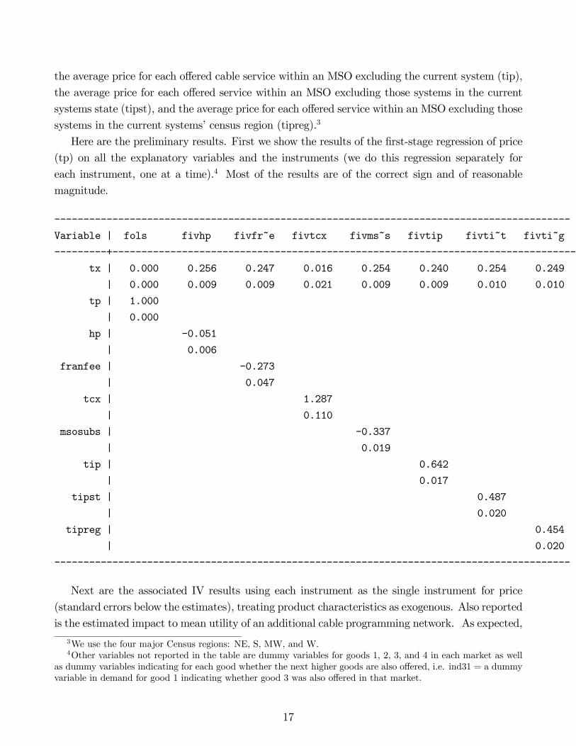
the average price for each offered cable service within an MSO excluding the current system (tip),
the average price for each offered service within an MSO excluding those systems in the current
systems state (tipst), and the average price for each offered service within an MSO excluding those
systems in the current systems’ census region (tipreg).3
Here are the preliminary results. First we show the results of the first-stage regression of price
(tp) on all the explanatory variables and the instruments (we do this regression separately for
each instrument, one at a time).4 Most of the results are of the correct sign and of reasonable
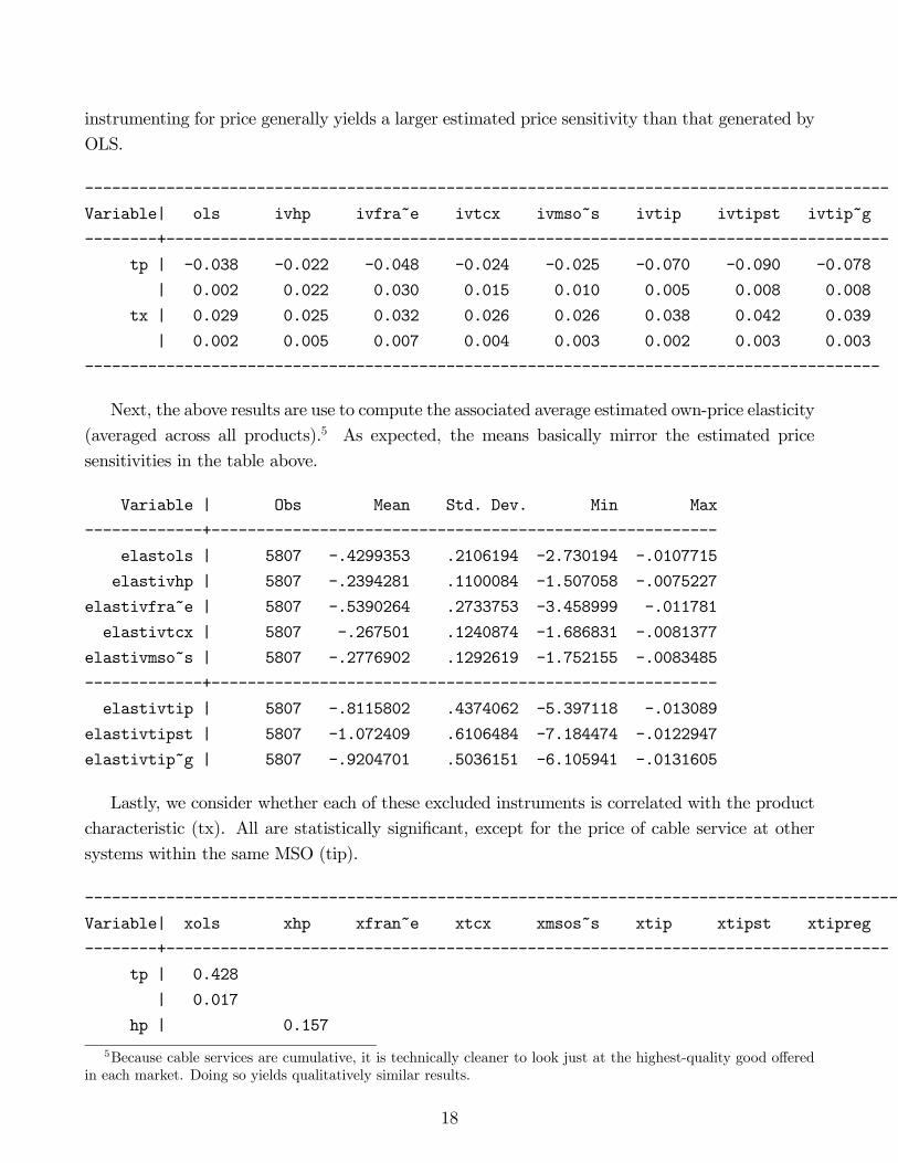
Next are the associated IV results using each instrument as the single instrument for price
(standard errors below the estimates), treating product characteristics as exogenous. Also reported
is the estimated impact to mean utility of an additional cable programming network. As expected,
3We use the four major Census regions: NE, S, MW, and W.4Other variables not reported in the table are dummy variables for goods 1, 2, 3, and 4 in each market as well
as dummy variables indicating for each good whether the next higher goods are also offered, i.e. ind31 = a dummyvariable in demand for good 1 indicating whether good 3 was also offered in that market.
17
instrumenting for price generally yields a larger estimated price sensitivity than that generated by
5Because cable services are cumulative, it is technically cleaner to look just at the highest-quality good offeredin each market. Doing so yields qualitatively similar results.
This suggest that the results using tip are likely to be the most reliable. We can formalize this
comparison using our upper bounds. In particular suppose we use (??) to calculate upper boundson the absolute value of the bias, imposing the assumption the assumption that 1
NX1MW <q
1NX1MWX1
q1NyMWy. we get the following bias bounds using the various instruments:
[1] Berry, S.T. “Estimating Discrete Choice Models of Product Differentiation.” RAND Journalof Economics, Vol. 25 (1994), pp. 242-262.
[2] –––—, and Pakes, A. “Estimating the Pure Hedonic Discrete Choice Model.” WorkingPaper, Yale University, 1999.
[3] –––—, Levinsohn, J.A., and Pakes, A. “Automobile Prices in Market Equilibrium.” Econo-metrica, Vol. 63 (1995), pp. 841-890.
[4] Bresnahan, T.F. “Competition and Collusion in the American Auto Industry: The 1955 PriceWar.” Journal of Industrial Economics, Vol. 35 (1987), pp. 457-482.
[5] –––—, T.F., Stern, S., and Trajtenberg, M. “Market Segmentation and the Sources of Rentsfrom Innovation: Personal Computers in the Late 1980s.” RAND Journal of Economics, Vol.28 (1997), pp. S17-S44.
[6] Chernozhukov, Imbens, and Newey (2006) "Instrumental Variable Estimation of Non-separable Models" Journal of Econometrics, 139, 1 4-14
[7] Crawford, G. “The Impact of the 1992 Cable Act on Household Demand andWelfare.” RANDJournal of Economics, Vol. 31 (2000), pp. 422-449.
[8] –––—, and Shum, M. (2006) "The Welfare Effects of Endogenous Quality Choice: TheCase of Cable TV", mimeo, Johns Hopkins
[9] Fan, Y. (2009) "Market Structure and Product Quality in the US Daily Newspaper Market",mimeo, Yale
[10] Goolsbee and Petrin (2004) "The consumer gains from direct broadcast satellites and thecompetition with cable TV", Econometrica, 72, 2. pp. 351-381
21
[11] Hausman, J. (1997) "Valuation of new goods under perfect and imperfect competition" inThe Economics of New Goods, NBER, edited by Tim Bresnahan and Robert Gordon
[12] Nevo, A. “Measuring Market Power in the Ready-to-Eat Cereal Industry.” Econometrica, Vol.69 (2001), pp. 307-342.
[13] Nevo, A. and Rosen, A. (2008) "Identification with Imperfect Instruments", NBER workingpaper
[14] Pioner, H. (2008) "Semiparametric Identification of Multidimensional Screening Models",mimeo, Chicago
[15] Sweeting, A (2008) "Dynamic Product Repositioning in Differentiated Product Industries:The Case of Format Switching in the Commercial Radio Industry", mimeo, Duke