ESTIMATING RESPIRATORY MOTION FROM CT IMAGES VIA DEFORMABLE MODELS AND PRIORS by Rongping Zeng A dissertation submitted in partial fulfillment of the requirements for the degree of Doctor of Philosophy (Electrical Engineering: Systems) in The University of Michigan 2007 Doctoral Committee: Professor Jeffrey A. Fessler, Chair Professor Alfred O. Hero Professor Charles R. Meyer Professor Randall K. Ten Haken Associate Professor James M Balter
Transcript
ESTIMATING RESPIRATORY MOTION FROM CTIMAGES VIA DEFORMABLE MODELS AND PRIORS
by
Rongping Zeng
A dissertation submitted in partial fulfillmentof the requirements for the degree of
Doctor of Philosophy(Electrical Engineering: Systems)
in The University of Michigan2007
Doctoral Committee:Professor Jeffrey A. Fessler, ChairProfessor Alfred O. HeroProfessor Charles R. MeyerProfessor Randall K. Ten HakenAssociate Professor James M Balter
1.2 Example of discontinuity artifacts seen in the 4D CTs acquiring from slice CT scanners.Pictures are borrowed from the paper by Keall et al. [33]. . . . . . . . . . . . . . . . . . . 4
2.7 A slice reconstructed from a GE 8-slice Lightspeed CT scanner (0.5 sec per rotation).Motionartifacts exist at around the edge of the mass in the left lung. . . . . . . . . . . . . . . . . 23
3.1 System model of the measurements. . . . . . . . . . . . . . . . . . . . . . . . . . . . . . 29
3.2 The X-ray projection image (a) and its CC gradient image (b). . . . . . . . . . . . . . . . 36
3.3 The absolute value of the gradient image (a) and its axial projection (b). . . . . . . . . . . 36
3.4 The image formed by combining the 1D axial projections. Each column corresponds to asingle 1D projection. . . . . . . . . . . . . . . . . . . . . . . . . . . . . . . . . . . . . . 36
3.5 An illustration of the extracted breathing signal borrowed from our later simulation re-sults. The solid line represents the true breathing signal and the dashed line represents theextracted breathing signal. . . . . . . . . . . . . . . . . . . . . . . . . . . . . . . . . . . 37
3.6 The three views of the reference thorax CT volume. (Points in the images are the projectionpositions on the three planes of the voxels randomly selected for accuracy plots . . . . . . . 40
3.7 Examples of simulated motion-included cone-beam projection views. From left to right,the projection angles are 28◦, 70◦, 112◦, 154◦. . . . . . . . . . . . . . . . . . . . . . . . . 40
3.8 Example of motion-free cone-beam projection views from angle 28◦, 70◦, 112◦, 154◦. . . . 42
5.2 This figure illustrates that normalization (5.12) of each estimated breathing index sequenceimproves robustness to imperfect reference volumes. . . . . . . . . . . . . . . . . . . . . 83
viii
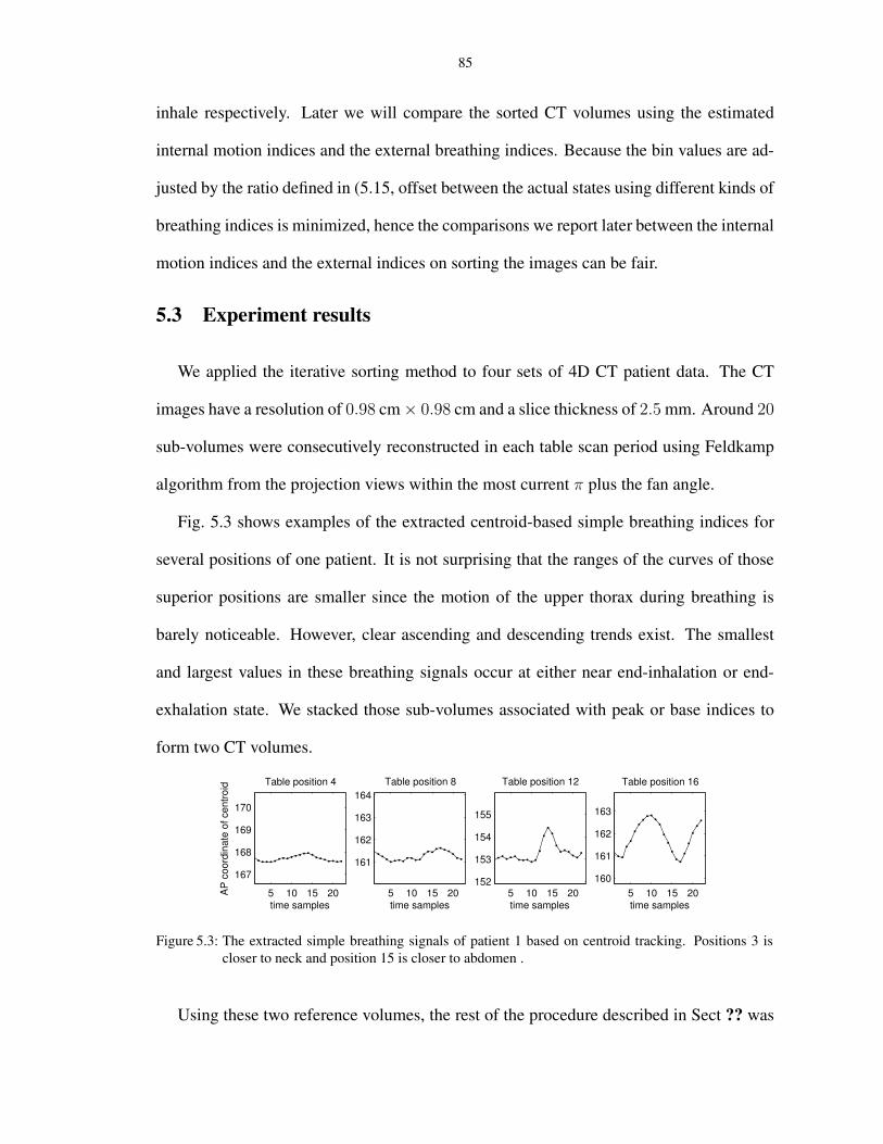
5.3 The extracted simple breathing signals of patient 1 based on centroid tracking. Positions 3is closer to neck and position 15 is closer to abdomen . . . . . . . . . . . . . . . . . . . . 85
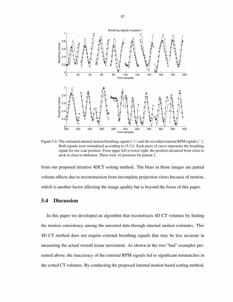
5.4 The estimated internal motion breathing signals (’+’) and the recorded external RPM sig-nals (’.’). Both signals were normalized according to (5.13). Each piece of curve representsthe breathing signal for one scan position. From upper left to lower right, the position ad-vanced from close to neck to close to abdomen. There were 16 positions for patient 1. . . . 87
5.5 The estimated internal motion breathing signals (’+’) and the recorded external RPM sig-nals (’.’) for patient 2. Both signals were normalized according to (5.13). Each piece ofcurve represents the breathing signal for one scan position. From upper left to lower right,the position advanced from close to neck to close to abdomen. There are 15 positions forpatient 2 . . . . . . . . . . . . . . . . . . . . . . . . . . . . . . . . . . . . . . . . . . . . 88
5.6 Sorted CT volumes of patient 1 using recorded RPM indices (a) and internal motion indices(b). From upper left to lower right, the patient exhale and then inhale. Severe tissuemismatches are marked by arrows. . . . . . . . . . . . . . . . . . . . . . . . . . . . . . . 89
5.7 Sorted CT volumes of patient 2 using recorded RPM indices (a) and internal motion in-dices (b). From upper left to lower right, the patient exhale and then inhale.Severe tissuemismatches are marked by arrows. . . . . . . . . . . . . . . . . . . . . . . . . . . . . . . 90
ix
LIST OF TABLES
Table
2.1 Comparison of TPS and B-spline registration results. MAE and σ are the mean and stan-dard deviation of the absolute errors of the the predicted coordinates of landmarks at inhalew.r.t the actual ones for each patient. cc is the correlation coefficients between the actualinhale and the predicted inhale based on registration. . . . . . . . . . . . . . . . . . . . . 16
3.4 The estimation accuracy of the LS estimator and the correlation-based estimator. The meanerrors and the standard deviations were calculated over the whole volume through time . . 52
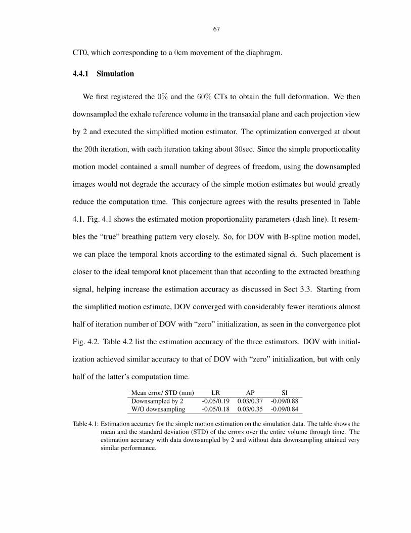
4.1 Estimation accuracy for the simple motion estimation on the simulation data. The tableshows the mean and the standard deviation (STD) of the errors over the entire volumethrough time. The estimation accuracy with data downsampled by 2 and without datadownsampling attained very similar performance. . . . . . . . . . . . . . . . . . . . . . . 67
4.3 Estimation accuracy of the simplified motion estimator, DOV with “zero” initialization andDOV starting from simplified motion estimates. The table shows the mean and the STD ofthe errors over the landmarks. . . . . . . . . . . . . . . . . . . . . . . . . . . . . . . . . . 69
x
LIST OF APPENDICES
Appendix
A. Calculations of the derivatives of the cost function ψ for B-spline based DOV . . . . . . . . . 100
A.1 Calculation of the gradient of ψ(θ) . . . . . . . . . . . . . . . . . . . . . . . . . . 100A.2 Calculation of ψ(α) and ψ(α) for line search . . . . . . . . . . . . . . . . . . . . . 101
xi
ABSTRACT
ESTIMATING RESPIRATORY MOTION FROM CT IMAGES VIA DEFORMABLEMODELS AND PRIORS
by
Rongping Zeng
Chair: Jeffrey A. Fessler
Understanding the movement of tumors during breathing is very important for conformal
radiotherapy. Without the knowledge of the tumor movement, it is likely that either in-
sufficient dose is delivered to tumors, or unnecessary dose is received by the surrounding
normal tissue, or both. However, respiratory motion is very difficult to study by conven-
tional x-ray CT imaging since object motion causes inconsistent projection views, leading
to artifacts in reconstructed images. This dissertation focused on developing methods to
build four-dimensional (4D) models of patient’s anatomy during breathing, especially in
thoracic and upper abdominal region, with currently available X-ray imaging techniques.
We explored methods to estimate respiratory motion from a sequence of cone-beam
X-ray projection views acquired using a slowly rotating cone-beam CT (CBCT) scanner
that was integrated into a Linac system. The slowly rotating CBCT scanners have a large
volume coverage and a high temporal sampling rate. In the proposed deformation from
orbiting views (DOV) approach, we modeled the motion as a time varying deformation
of a static reference volume of the anatomy. We then optimized the parameters of the
motion model by maximizing the similarity between the modeled and actual projection
xii
views. The modeled projection views were calculated by deforming the reference volume
according to a parametric, four-dimensional (4D) B-spline motion model and projecting
the deformed volumes onto the detector coordinates corresponding to the actual measured
projection views. Challenges of this estimation problem include the limited gantry rotation
in one breathing cycle, Compton scatter contamination of the projection views and heavy
computation, which will be addressed in the dissertation. We conducted computer sim-
ulations and a phantom experiment to test the performance of this approach. Both cases
achieved estimation accuracies within voxel resolution. We also investigated the effects of
several factors, such as the temporal knot placement and regularization parameters, on the
estimation accuracy. Long computation time would limit the clinic usage of this method.
So we explored methods that accelerate the optimization procedure.
We researched the 4DCT imaging methods using multi-slice CT (MSCT) scanners and
proposed a method to find the temporal correspondences among the unsorted 4DCT im-
ages based on internal anatomical motion. Our method used all the CT slices at each table
position to estimate internal motion-based sorting indices, Patient studies showed that the
internal motion-based sorting greatly reduced tissue mismatch presented in the formed CT
volumes using the externally recorded surrogates of breathing motion.
xiii
CHAPTER 1
Introduction
1.1 One big challenge in radiation therapy: respiratory motion
In 2006, more than 160, 000 people died from lung cancer in United States. That is more
than the next four leading causes of cancer death - colon, breast, pancreas and prostate -
combined, according to the American Cancer Society. Effective and efficient lung can-
cer treatment is critical. Surgical remover, chemotherapy and radiation therapy are three
main methods of lung cancer treatment. The work presented in this dissertation aims at
improving the accuracy and efficiency of the third method, radiation therapy of patients,
especially for the patients with lung cancer.
It has been reported that respiratory motion causes significant movement of tumors in
thoracic and abdominal region [3, 79]. Many tumors in those region may move as much
as 3 cm peak-to-peak during radiation treatment. Such large geometric uncertainties have
posed a big challenge to conformal radiotherapy treatment of patients with lung cancer.
Conformal radiotherapy requires that radiation dose is precisely delivered to tumors while
sparing adjacent normal tissue. Techniques such as Intensity Modulated Radiotherapy
(IMRT) (Fig. 1.1). use sophisticated software and multi-leaf collimator to shape the radi-
ation beam and change the intensity within each beam to deliver optimum doses. This de-
mands accurate tumor and critical structure delineation. Lack of knowledge of respiration
1
2
induced motion possibly results in either insufficient dose to tumors, unnecessary dose to
surrounding healthy tissue, or both. Although treatment can be done under breathhold con-
dition by forcing patients to breathe shallowly or hold their breath by instruments [63,95],
such type of treatments is very uncomfortable and even impossible for some patients with
lung cancer, who may have difficulty holding their breath.
Beam Tumor (orange)
Figure 1.1: Illustration of IMRT
Accounting for motion should improve the effectiveness and efficiency of radiother-
apy treatment. This can be achieved by the following techniques. One is to incorporate
the anatomical movement into treatment planing, rather than adding standard margin, to
reduce the total lung dose received by the patient [64,74,84]. The second type is gated ra-
diotherapy [78,86], in which the treatment plan is designed based on the tumor position in
a certain phase and during treatment the beam is turned on in that phase and turned off oth-
erwise. Another technique is the so-called four-dimensional (4D) radiotherapy, in which
the shape and the intensity of the beam is continuously adjusted to follow the movement
of tumors throughout the whole breathing cycle [32, 94]. All those techniques require the
knowledge of how the patient’s anatomy moves during breathing.
3
1.2 Current 4D CT imaging methods
To obtain a complete picture of the patients’ anatomy at all times during breathing,
intensive work has been dedicated to four-dimensional (4-D) computed tomography (CT)
(three-dimensional (3D) space + one-dimensional (1D) time or breathing phase ) imaging
techniques [33, 44, 48, 55, 58, 66, 77, 87, 96]. With the availability of 4D CT, deformation
maps during breathing can be estimated by registering those CT volumes.
4D CT images can be acquired using either slice (single or multi-slice) CT scanners
or cone-beam CT (CBCT) scanners. Slice CT scanners usually rotate very fast but have
very limited axial coverage ( 2 − 4 cm) [39]. 4DCT imaging techniques using slice CT
scanners often acquire multiple two-dimensional (2D) slices at each table position, sort
these slices into several respiratory phase bins, and then stack those slices that are within
the same phase bins to form a 4D model [48,58,87]. Most current sorting methods depend
on an externally recorded breathing index associated with each CT slice. This sorting pro-
cess validates on the assumption that the internal motion is reproducible with the external
breathing index. Real respiratory motion is irregular. Correlation between the external
breathing index and the internal anatomical motion is often imperfect, leading to discon-
tinuity artifacts in the sorted CT volumes, as shown in the example in Fig. 1.2 [33]. On
the other hand, CBCT scanners have large axial coverage but rotate very slowly (1 min
per rotation). Because of the slow rotation of CBCT, 4DCT imaging methods using such
scanners also require a pre-sorting of the projection views into certain phase bins and
then reconstruct 3D CT volumes using subsets of the projection views corresponding to
the same phases [44, 66, 77]. Assumption of motion reproducibility remains a limitation.
Moreover, insufficient numbers of projections per breathing phase may also result in se-
vere artifacts in the reconstructed images, such as low contrast-to-noise ratio, blurring and
4
streak artifacts. Rit et al. conducted experiments to study the effect of the number of
phase bins on the temporal and spatial resolution of the 4DCT reconstruction using CBCT
scanners [66].
Figure 1.2: Example of discontinuity artifacts seen in the 4D CTs acquiring from slice CT scanners. Picturesare borrowed from the paper by Keall et al. [33].
Those 4DCT imaging techniques are very helpful in unveiling internal anatomical
movement caused by respiratory motion. However, limitations still exist, such as the mo-
tion reproducibility assumption with respect to the breathing index and insufficient projec-
tion views for 3D volume reconstruction. Degraded image quality due to those limitations
jeopardizes the accuracy of treatment planning. Our effort in this dissertation is toward
building 4D CT models that can better describe respiratory motion with high temporal and
spatial resolution and with less distortion.
1.3 Thesis outline and contributions
In this dissertation, we propose two methods to build 4D patient-specific respiratory
motion models: the deformation domain and the image domain.
• Iterative approach to estimate respiratory motion from a sequence of slowly rotating
cone-beam projection views.
This method models the motion as a time-varying deformation of a reference volume
and estimates the motion parameters by maximizing the similarity between the mod-
5
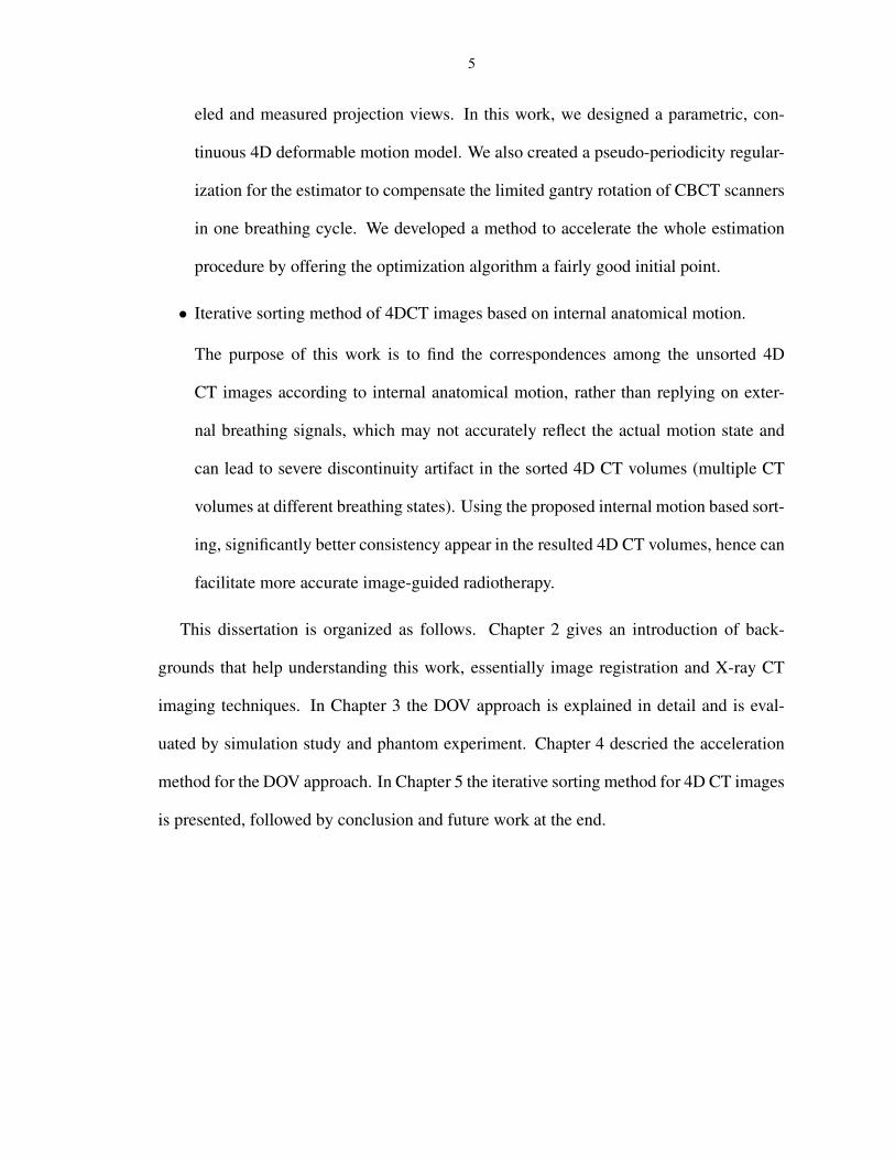
eled and measured projection views. In this work, we designed a parametric, con-
tinuous 4D deformable motion model. We also created a pseudo-periodicity regular-
ization for the estimator to compensate the limited gantry rotation of CBCT scanners
in one breathing cycle. We developed a method to accelerate the whole estimation
procedure by offering the optimization algorithm a fairly good initial point.
• Iterative sorting method of 4DCT images based on internal anatomical motion.
The purpose of this work is to find the correspondences among the unsorted 4D
CT images according to internal anatomical motion, rather than replying on exter-
nal breathing signals, which may not accurately reflect the actual motion state and
can lead to severe discontinuity artifact in the sorted 4D CT volumes (multiple CT
volumes at different breathing states). Using the proposed internal motion based sort-
ing, significantly better consistency appear in the resulted 4D CT volumes, hence can
facilitate more accurate image-guided radiotherapy.
This dissertation is organized as follows. Chapter 2 gives an introduction of back-
grounds that help understanding this work, essentially image registration and X-ray CT
imaging techniques. In Chapter 3 the DOV approach is explained in detail and is eval-
uated by simulation study and phantom experiment. Chapter 4 descried the acceleration
method for the DOV approach. In Chapter 5 the iterative sorting method for 4D CT images
is presented, followed by conclusion and future work at the end.
CHAPTER 2
Background and Preliminaries
2.1 Review of Registration
The purpose of image registration is to find a geometrical relationship between two
objects. Image registration has been extensively studied in recent years [7, 24, 40, 43, 54,
56,82,83]. It is widely applied in the medical image domain, such as, analyzing the tumor
changes before and after treatment, tracking the neural activity in the fMRI images, fusing
images with different modalities (CT, PET, MRI etc.) to enable more accurate diagnosis.
Other than the medical domain, image registration is also an important tool for the area of
computer vision, such as motion analysis and object tracking.
Image registration is defined as follows. Given two objects, the reference image fref(x)
and the target image ftar(x), where x ∈ Rd and d is the number of dimensions of the
objects, the task of image registration is to determine a geometric transformation T that
aligns each point in fref(x) with the corresponding point in ftar(x). From this definition,
image registration includes two essential parts, representation of geometric transforma-
tions and measure of alignment between two images (i.e., similarity measure), which we
describe next.
6
7
2.1.1 Classification of geometric deformations
Geometric transformations can be partitioned into rigid transformations and nonrigid
transformations. The latter one can be further divided into affine transformations and
curved transformations. Some literatures may consider rigid transformations as a subclass
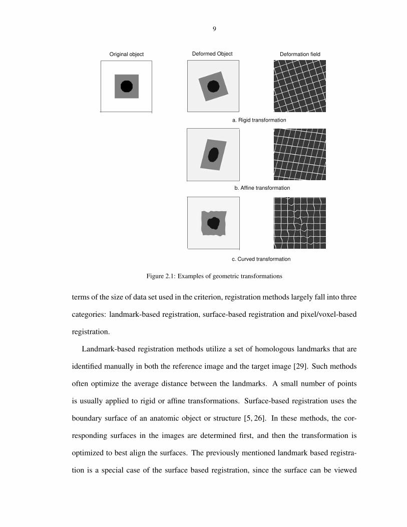
of affine transformations because both types are linear. Fig. 2.1 shows examples for each
of these three transformation types.
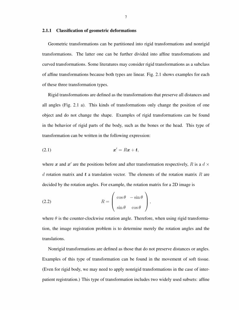
Rigid transformations are defined as the transformations that preserve all distances and
all angles (Fig. 2.1 a). This kinds of transformations only change the position of one
object and do not change the shape. Examples of rigid transformations can be found
in the behavior of rigid parts of the body, such as the bones or the head. This type of
transformation can be written in the following expression:
(2.1) x′ = Rx + t,
where x and x′ are the positions before and after transformation respectively, R is a d ×
d rotation matrix and t a translation vector. The elements of the rotation matrix R are
decided by the rotation angles. For example, the rotation matrix for a 2D image is
(2.2) R =
cos θ − sin θ
sin θ cos θ
,
where θ is the counter-clockwise rotation angle. Therefore, when using rigid transforma-
tion, the image registration problem is to determine merely the rotation angles and the
translations.
Nonrigid transformations are defined as those that do not preserve distances or angles.
Examples of this type of transformation can be found in the movement of soft tissue.
(Even for rigid body, we may need to apply nonrigid transformations in the case of inter-
patient registration.) This type of transformation includes two widely used subsets: affine
8
transformations and curved transformations.
Affine transformations preserve the straightness and parallelism of lines, but allow
changes on angles between lines (Fig. 2.1 b). They can be represented by
(2.3) x′ = Ax + t,
where A is an d× d matrix. There is no restriction on the elements of the matrix A, unlike
the rotation matrix R in rigid transformations in which the elements are dependent to each
other through the rotation angles. Registration problems using affine transformations also
only need to decide a few parameters.
Curved transformations, also called elastic transformations, do not require the preser-
vation of angles or lines (Fig. 2.1 c). They are the most common transformations seen in
soft tissue, such as the liver, heart, thorax etc. In most applications, these transformations
are described using a local deformation field D,
x′ = x + D(x).
Since the deformation of the anatomy is generally smooth, it is reasonable to represent the
local deformation field as a sum of shifted basis functions:
(2.4) D(x) =∑
i
cib(x − i)
where b(x) is a basis function and ci values are the coefficients. There are various choices
on the basis functions, such as polynomial functions, radial functions and spline functions.
Registration using curved transformation often involves a large number of parameters to
be determined.
2.1.2 Registration methods
Registration problems are usually solved by iteratively optimizing some criterion or
some similarity measure between the target object and the deformed reference object. In
9
Original object
a. Rigid transformation
Deformation field
b. Affine transformation
c. Curved transformation
Deformed Object
Figure 2.1: Examples of geometric transformations
terms of the size of data set used in the criterion, registration methods largely fall into three
categories: landmark-based registration, surface-based registration and pixel/voxel-based
registration.
Landmark-based registration methods utilize a set of homologous landmarks that are
identified manually in both the reference image and the target image [29]. Such methods
often optimize the average distance between the landmarks. A small number of points
is usually applied to rigid or affine transformations. Surface-based registration uses the
boundary surface of an anatomic object or structure [5, 26]. In these methods, the cor-
responding surfaces in the images are determined first, and then the transformation is
optimized to best align the surfaces. The previously mentioned landmark based registra-
tion is a special case of the surface based registration, since the surface can be viewed
10
as a large set of points. Determination of the surface can be semi-automatic or fully au-
tomatic and these registration methods can be applied to both rigid transformations [26]
and nonrigid transformations [73]. However, a difficult problem related to the nonrigid
surfaced based registration is how to interpret the relationship between the deformation
of the internal points and the surface points. Pixel/voxel based image registration works
differently from the previous two classes in that it operates directly on the image intensity
values [40,61,82]. It has recently become the most interesting registration basis in medical
imaging applications, since these methods are fully automatic and can be applied to both
rigid and nonrigid transformations. The transformations are often found by iteratively op-
timizing some similarity measure calculated from the pixel/voxel intensity values, such
as the sum of squared differences, correlation coefficients, or mutual information. The
intensity-based method can also include the landmark, surface or shape feature as part of
its similarity measure to increase the accuracy of registration [27, 89].
2.1.3 Regularizations on image registration
Curved transformations are more general in representing human anatomy deformation.
Because the large number of parameters associated with curved transformations as well
as measurement noise, elastic registration problems tend to be ill-posed, i.e., there exist
many local minima which may be nonrealistic. Therefore regularizations are neccessary
for such registration problems. Accordingly, the cost function that a registration algorithm
intends to optimize includes some similarity terms of the two objects and regularization
terms on the deformation estimates. The similarity metrics have been discussed in the
previous section and here we briefly introduce choices on deformation regularizations.
Regularazations are usually designed based on some physical properties of the human
anatomical deformation. The following properties have been considered in the literature
11
of elastic registration. Smoothness regularization, which can be measured by the deriva-
tives of the deformation field, encourages slow changes of movement between neighbor-
ing voxels. Invertibility regularization discourages folding. To penalize such undesired
deformation estimates, one may penalize negative Jacobian values of the estimated defor-
mation [35]. Consistency regularization encourages the deformations that aligns object A
to B and aligns B to A to be the same. To pose this regularization, one may register A to B
and B to A simultaneously and penalize the differences between the deformation estimates
of the two directions but then neither is accurate [7, 22, 27]. Other than those global prop-
erties of human’s anatomical deformation, local rigidity or imcompressibility according to
different types of tissue is also considered in registration [45,46,70,72,91]. The rigidity of
deformation can be measured by the deviation of Jacobian from an identity matrix. Such
penalties discourage elasticity at the rigid tissue such as bone. The imcompressibility or
volume-preservation property can be measured by the deviation of the determinant of Ja-
cobian from unity. It discourages expansion and compression of soft tissue such as liver
and breast.
2.1.4 Comparison of TPS and Cubic B-spline deformation models
Because the nonrigid deformation of thorax is our focus in this dissertation, here we
compare two deformation models used widely to describe anatomical deformation caused
by breathing: thin-plate spline (TPS) deformation model and cubic B-spline deformation
model. The two models have the different choices for the basis function b(x) in Eq. (2.4)
TPS deformation model
For TPS deformation model, the basis function is
U(x) = −‖x‖2 log(‖x‖2), (2D cases)
U(x) = ‖x‖ , (3D cases)(2.5)
12
where ‖x‖2 = x2 + y2 for 2D cases and ‖x‖2 = x2 + y2 + z2 for 3D cases, U is defined
to have value 0 at the origin, where log is not defined for 2D cases. This basis function
is the so-called fundamental solution of the biharmonic equation 42U = 0. Solutions
of the biharmonic equation represent the form that a thin-plate of metal would take when
forced through certain fixed points with lowest physical bending energy, thus the name of
thin-plate spline. The actual 3D TPS interpolation map between two sets of landmarks
decomposes into two parts, an affine part and the principle warps as follows,
x′ = ax0 + ax
1x+ ax2y + ax
3z +n∑
i=1
cxi U(‖Pi − (x, y, z)‖),(2.6)
y′ = ay0 + ay
1x+ ay2y + ay
3z +n∑
i=1
cyiU(‖Pi − (x, y, z)‖),(2.7)
z′ = az0 + az
1x+ az2y + az
3z +n∑
i=1
cziU(‖Pi − (x, y, z)‖),(2.8)
where Pi denotes the coordinate of landmark i, (x, y, z) and (x′, y′, z′) the coordinates
before and after transformation, and ax, ay,az, cx, cy , cz are coefficients. Given two sets of
landmarks, one in the reference image and another homologous one in the target image, the
coefficients can be found by solving equation arrays formed by substituting the landmark
coordinates into (2.6), (2.7) and (2.8) [6]. For medical image registration applications, the
landmarks are usually identified based on specific anatomical structures.
B-spline motion model
B-splines are smoothly connected piecewise polynomials. Specifically, here we refer it
to the most widely used B-spline function of degree n = 3, which is called cubic B-spline.
Its close-form expression is as follows,
(2.9) β(x) =
23− |x|2 + |x|3
2, 0 ≤ |x| < 1
(2−|x|)3
6, 1 ≤ |x| < 2
0 |x| ≥ 2
13
The d-dimensional basis is defined to be the tensor product of the 1D cubic B-spline, i.e.,
(2.10) β(x) =D∏
d=1
β(xd),
A 3D B-spline deformation model, indcluding a identity part and an warping part, is ex-
pressed as follows,
x′ = x+K∑
k=1
J∑
j=1
I∑
i=1
cxijk β
(x− xi
hx
)
β
(y − yj
hy
)
β
(z − zk
hz
)
,(2.11)
y′ = y +K∑
k=1
J∑
j=1
I∑
i=1
cyijk β
(x− xi
hx
)
β
(y − yj
hy
)
β
(z − zk
hz
)
,(2.12)
z′ = z +K∑
k=1
J∑
j=1
I∑
i=1
czijk β
(x− xi
hx
)
β
(y − yj
hy
)
β
(z − zk
hz
)
,(2.13)
where {xi}, {yj}and{zk}) are the coordinates of the B-spline control knots, and hx, hy and
hz specify the the width of the B-spline function. The control knots are usually uniformly
distributed along each dimension, but one may also use nonuniform control grids. The
density of the control grids can be different for various applications. B-spline model with
a denser control grid will be able to describe signals containing higher frequency, or signals
that change more rapidly. Theory has also been established that B-splines could be a good
interpolator for continuous signals [85]. With the advance of computer techniques, B-
spline has caught more and more interest in engineers.
Comparison of TPS and B-spline deformation models
A direct comparison of the basis function (2.5) and (2.9) gives an obvious difference
between these two models, i.e., TPS basis has an infinite support while B-spline has a
very short support. Hence, changes at each knot will exert a global effect on the whole
deformation for the TPS model, while only a local effect for the B-spline model. In this
sense, B-splines should perform better at modeling local and subtle deformations.
To compare the performance of these two models in approximating the deformations of
14
thorax, We conducted the following registration experiment on 11 pairs of inhale and ex-
hale thorax CT volumes, all with voxel size 0.19× 0.19× 0.51cm3. First, thin-plate spline
registration was used to align the inhale and exhale CTs, yielding a TPS deformation field.
Then we did a least square fitting of the TPS field into a cubic B-spline deformation field
and registered the same pair of CTs using the B-spline model starting from the fitted defor-
mation field. This registration yielded a B-spine deformation field. We compared the two
registration results to see if the B-spline model could improve registration accuracy, which
was evaluated by the differences of the actual and predicted positions of six landmarks.
These landmarks were carefully identified by experts from the locations of vascular and
bronchial bifurcations [11].
TPS registration was conducted by M. Coselmon et al. [9]. For the TPS registration,
30 control points were used to align the inhale CT to exhale CT. The control points were
manually chosen in both the inhale and exhale CTs. Control points in the inhale CT
were fixed, while control points in the exhale CT were perturbed in the whole registration
procedure. At each iteration, the coordinates of the control points in exhale CT were
updated to maximize the mutual information (MI) between the inhale CT and the deformed
exhale CT. Optimization method was the Nelder-Mead simplex algorithm. Registration
stopped when the MI change in three consecutive iterations had not exceed a threshold.
B-spline registration was implemented based on the code written by J. Kim [34]. For
the B-spline registration, mean of squared differences was used as the registration crite-
rion. The estimator was regularized to limit negative Jacobian determinant, which implies
nonrealistic anatomy deformations such as folding and splitting. We chose the B-spline
knots to be evenly distributed in the region of interest spacing by 16, 16 and 4 pixels along
left-right (LR), anterior-posterior (AP) and superior-inferior (SI) direction respectively.
The coefficient value at each knot was optimized using the Gradient Descent algorithm.
15
Registration stopped when the criterion had dropped down to a threshold.
Since we were interested in the right lung only, masking was done to restrict the regis-
tration on the right lung. Computation time was saved by this masking image registration.
Table 2.1 summarizes the registration accuracy results for TPS and B-spline registration,
including comparisons of the mean difference, standard deviation and correlation coeffi-
cient between the actual and predicted landmark positions. As can be seen in this table,
B-spline registration resulted in accuracy improvement in most cases, with a decrease of
mean absolute differences up to 3mm in case 6. Also the correlation between the actual
and the predicted inhale CTs were much higher for B-spline registration than for TPS reg-
istration. The improvement achieved by B-spline registration indicates that the B-spline
deformation model has better than or at least equal performance with the TPS deformation
model in approximating thorax deformations caused by breathing. Moreover, the property
of local support of B-splines could save computation time and reduce the complexity of
optimization. These two advantages support our decision to use the B-spline model for our
later respiratory motion estimation problem, in which we deform a breathhold CT volume
through time to match its projection views to the measured sequential projection views,
which we view as a kind of “tomographic image registration” problems.
Computed Tomography (CT) is a non-invasive imaging technique allowing the visual-
ization of the internal structure of an object. In a CT system, the patient is placed between
an X-ray source and an array of X-ray detectors. By rotating the source and the detector
simultaneously around the patient, a large number of X-ray projections from different an-
gles can be obtained during the data acquisition period. Ideally, each projection represents
16
Table 2.1: Comparison of TPS and B-spline registration results. MAE and σ are the mean and standarddeviation of the absolute errors of the the predicted coordinates of landmarks at inhale w.r.t theactual ones for each patient. cc is the correlation coefficients between the actual inhale and thepredicted inhale based on registration.
Patient No. TPS registration B-spline registrationMAE σ cc MAE σ cc
Most CT image reconstruction algorithms assume that the object does not move during
the scan. This stationary condition is violated when there exists organ motion during the
scanning process and the collected projections are inconsistent. This inconsistency leads
to severe artifacts in the reconstructed images, such as blurring, partial volume, and streak
artifacts, especially for organs in thorax and abdomen regions where may present up to
3cm tissue movement. There are various methods being developed to reduce motion arti-
facts in the reconstructed images.. They can be largely divided into three categories: fast
scanning, reconstruction for motion compensation and gated image acquisition. In the first
class, researchers endeavor to shorten scanner rotation times for data acquisition to reduce
motion artifacts and improve temporal resolution [25, 67, 68]. For slice CT scanners, it
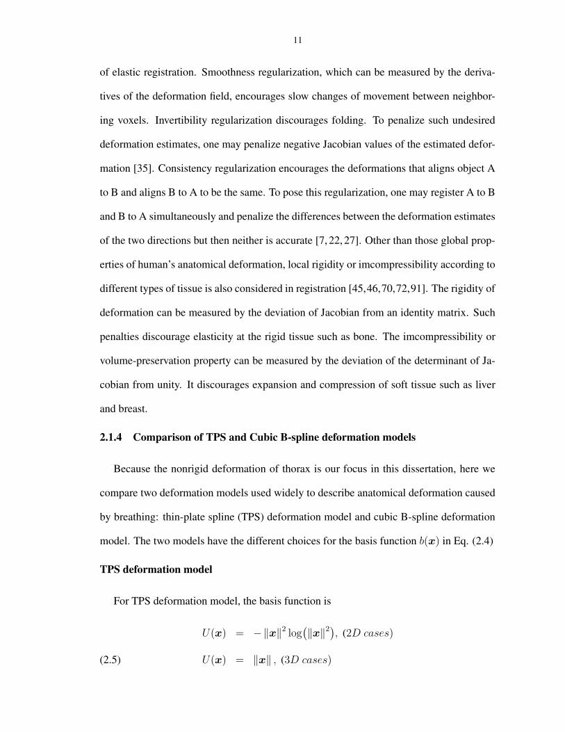
can rotate as fast as 0.5 sec per rotation and projections of slightly larger than half rotation
are sufficient for one reconstruction. Even with this fast scanner, motion artifacts are still
present in the reconstructed images, as shown in Fig. 2.7. In the second class, reconstruc-
tion algorithms for motion compensation are based on assumptions of a prior deformation
23
model [10, 71, 88], or based on the estimation or detection of motion using extra hard-
ware [16, 49] or from extra data set [44]. In most of these work, only the deformation
models that preserve lines are considered. However,the movement of human anatomy are
much more complex than those line-preserved deformation models. In gated image acqui-
sition techniques, which are designed for 3D CT volume reconstruction, devices are used
to measure the breathing state either as a trigger signal to initiate the scan to acquire data
at a certain breathing state [20], or as a metric to sort the CT scans into bins of equivalent
breathing states to form a volume [48, 87]. However, this type of methods highly depend
on the reproducibility of the organ motion with respect to the external breathing index.
Moreover, the 2D slices that are stacked tot form a 3D volume may still contain motion
artifact. Rather than working on motion reduction directly, in DOV, the method we will
present in the next chapter, we use those motion-included projection views to estimate the
anatomy motion, assuming available a static reference volume of the anatomy such as a
breathhold treatment planning CT. With the motion estimated by DOV and a reference
volume, 4D CT images can be generated by deforming the reference volume according to
the estimation motion.
Figure 2.7: A slice reconstructed from a GE 8-slice Lightspeed CT scanner (0.5 sec per rotation).Motionartifacts exist at around the edge of the mass in the left lung.
CHAPTER 3
Respiratory motion estimation from sequential X-ray cone-beamprojection views (DOV)
This chapter describes one of the main work of this dissertation, a method that estimates
respiratory motion using a deformable motion model from a static reference volume and
a sequence of slowly rotating, free-breathing projection views. We name is Deformation
from Orbiting Views (DOV). It is essentially a dynamic 3D-2D registration method. 3D-
2D image registration had been widely used for patient set up estimation in radiotherapy
system. It compares the digitally rendered radiographs (DRR) of the 3D treatment plan-
ning CT volume to fluoroscope or electronic portal images to optimize a rigid patient setup
difference [37, 42, 60]. In our dynamic 3D-2D registration, we simutaneously optimize a
sequence of time dependent nonrigid deformations to register a 3D CT volume to a se-
quence of 2D proejction views, which is much more challenging than the common 3D-2D
registration problems.
Building 4D patient-specific deformable models has attracted considerable attention in
these several years. A straightforward method is to register a 3D CT volume with 4D
CT volumes which contain multiple 3D CT volumes each at a pre-defined breathing state
over the respiratory cycle. However, limitations on current 4D CT imaging techniques,
which has been briefly mentioned in Chapter 1 and will be further discussed in Chapter 4,
will certainly extend into the deformation models estimated from those 4D CT volumes.
24
25
McClelland et al. [55] proposed method to build 4D motion model directly from a high
quality reference volume and the unsorted 4D CT images which contain free breathing
multi-slice CT “slabs”(2 − 3 cm thick) at each axial table position. They first registered
the reference volume to each of the free-breathing CT slab using B-spline based free-form
deformation, then constructed motion model by a temporal fitting of the registration results
over one respiratory cycle, assuming they have available the phase position at which each
slab was acquired, for example, from an externally monitored breathing index. Finally
they concatenate the motion model of each slab to form a 4D motion model of the whole
volume. It is a novel method and can provide one cycle of 4D motion model averaged
over a couple of respiratory cycles, which can facilitate automatic target propagation and
combining of dosed over one breathing cycle. The averaged motion model indicates that
this 4D motion model is not really along the natural time axis, but along a parameterized
time axis. Moreover, the registration step were operated separately on each small volumes
of 2− 3 cm thickness, hence the registration result may be less stable and robust; the con-
catenation step may also yield discontinuity artifacts at the slab boundaries. In our DOV
method, we dynamically register a sequence of projection views spanning over multiple
breathing cycles to a high quality reference CT volume, and we use a B-spline based mo-
tion model which is continuous in both time and space domain. Hence the so estimated
motion model are with the natural time axis and is also consistent in the spatial domain
because of no concatenation necessary in our method.
Most of the content in this chapter can be found in our recently published papers
[101, 102]. We explain the theory of DOV and then present our simulations and phan-
tom experiment.
26
3.1 Theory
DOV is a method that estimates respiratory motion, a sequence of time-dependent de-
formations, from a sequence of slowly rotating X-ray cone beam projection views with
the availability of a static reference CT volume. Estimation is often an inverse procedure
aimed at recovering some unknown parameters from available measurements. Generally,
for an iteratively solved estimation problem, there are three main tasks: define a suitable
system model that describes the mathematical relationship among the inputs and the pa-
rameters, choose a good cost function of the parameters according to the system model,
and select appropriate optimization algorithms to find the values of parameters that mini-
mize or maximize the cost function. Accordingly, we explain the DOV frame work from
these three points.
3.1.1 The system model
The proposed motion estimation method uses two sets of data. One is a reference tho-
rax CT volume obtained from a conventional fast CT scanner under breathhold conditions,
denoted fref(x),x ∈ R3. The other is a sequence of projection views of the same patient
acquired at treatment time using a slowly rotating cone-beam system (1 minute per rota-
tion), denoted Ym, m = 1, . . . ,M (M is the number of projection views). We establish
the relationship between the two data sets fref(x) and Y in this section.
We need to first address one concern about the slowly rotating cone-beam systems.
Although the cone-beam scanners rotate slowly, the acquisition time of each projection
view is short. For example, recently developed systems can acquire 15 frames per sec-
ond, which indicates that the imaging time for each frame is less than 0.067 second. We
therefore assume that the respiratory motion is negligible within each single projection
view.
27
Let the motion during the scan be denoted as T θ(x; t), a time-dependent deformation
controlled by parameters θ. Since the projection views and the reference volume are all
from the same patient, the ideal projection views gm can be related to fref in terms of the
CT imaging principle through the motion as follows,
gm = Aφmftm ,(3.1)
ftm(x) = fref(T θ(x; tm)),(3.2)
where Aφmdenotes the X-ray projection [53] operator for projection angle φm, and ftm is
the deformed volume at time tm. Combining (3.1) and (3.2), we obtain
(3.3) gm = Aφmfref(T θ(·; tm)).
However, in practice the projection views gm are estimated from the measured photon
counts Ym, which are always degraded by noise, dominated by the Poisson effect [1]. For
simplicity, we assume a monoenergetic model to describe the relationship between gm and
Ym as follows,
(3.4) Ym,n ∼ Poisson(Im,ne−gm,n + Sm,n),
where Im,n is a constant related to the incident X-ray intensity, Sm,n denotes the scatter
contribution to Ym,n and n is the detector element index. Then the projection views used
for DOV can be estimated from Ym as follows,
(3.5) gm,n = log
(
Im,n
Ym,n − Sm,n
)
.
In (3.5), Im,n can be measured by an air scan and Sm,n is an estimate of the scatter contri-
bution. There are a few popular ways to estimate scatter. One is to model the scatter as the
convolution of a function with the primary counts. The function could be approximated
by an exponential or Gaussian kernel [47]. Another way is to measure the scatter effect
28
using a beam stop array [57]. One may also estimate the scatter by using the Monto-Carlo
simulation method [8]. The DOV method can use any such scatter estimates.
We need to choose a deformation model to complete (3.3). Usually the movement of
tissue caused by breathing is nonrigid and smooth, except the case of sudden cough or
sneeze, which should be avoided during data acquisition. Therefore the anatomy deforma-
tion during breathing can be characterized by smooth curved transformations, which can
be approximated by a sum of weighted shifted basis functions as described in 2. Since the
temporal movement of anatomy also has the smoothness property, we adopt the following
B-spline based motion model,
(3.6) T θ(x; t) = x +∑
j
∑
i
θj,i β
(t− τj
∆t
)
β
(x − xi
∆x
)
,
where β(·) is the cubic B-spline function and β(x) the tensor product of cubic B-spline
functions, i.e., β(x) =∏D
d=1 β(xd), x = (x1, · · · , xD), τj and xi the spatial and temporal
knot locations, ∆x and ∆t control the width of the spatial and temporal basis functions re-
spectively, and θ the knot coefficients. There are two advantages of using a cubic B-spline
model. One is that the small support of the cubic B-spline function eases the computation
and optimization. The other is that the density of a B-spline control grid can be locally ad-
justed according to the characteristics of the signal to be fitted. For example, one can place
more knots at regions where the signal changes faster and less knots otherwise. Although
we use a B-spline based motion model, T θ(x; t) generalizes to any other suitable repre-
sentations. Note that in (5.2) T θ(x; t) contains motions in three orthogonal directions,
each controlled by a group of B-spline coefficients. Take the motion in the x-direction for
example,
(3.7) T xθ (x; t) = x +
∑
j
∑
i
θxj,i β
(t− τj
∆t
)
β
(x − xi
∆x
)
,
In Equation (3.3) the deformation is operated on a continuous reference image fref(x).
29
But the actual reference CT volume we obtain is discrete, therefore we need to interpolate
it to a continuous signal. Again, we chose the uniform cubic B-splines to interpolate the
discrete reference volume as follows,
(3.8) fref(x) =∑
i
ci β(x − i) .
ci are set such that we have a perfect fit at integers, i.e., the intensity value of fref(x) is
exactly the same as that of the discrete reference image at each integer pixel. They can be
solved conveniently by the digital filtering approach as described in [85].
To sum up, we established the relationship between the two measurements that are used
by DOV in this section. The following block diagram summarized this relationship. In this
block diagram we treat all the noise and artifacts caused by data acquisition as additive
noise. Based on the motion model (5.2), the estimation goal is to find the motion parame-
ters θ, containing three groups of knot coefficients for the three directions {x, y, z}, from
the projection views gm and the reference volume fref.PSfrag replacements
fref ft = fref(Tθ(x; t))g
Tθ(x; t) A
Motion Model Projection
Noise ε
Figure 3.1: System model of the measurements.
3.1.2 Regularized least-square estimator
As stated above, we need to find the motion parameters from a sequence of projection
views and a static anatomy prior of the patient. There is no analytical solution to this
problem. Moreover, the problem is ill-posed. Usually for such inverse problems, the
unknown parameters are solved by minimizing or maximizing a cost function based on
30
the system model. For an ill-posed inverse problem, i.e., a problem whose solution is
not unique or does not exist for arbitrary data or does not continuously depend on data,
a prior information is often necessary to “reject” those unrealistic answers [4]. Thus the
cost function usually contains regularization terms besides data fidelity terms.
DOV is essentially a registration problem. But unlike the traditional image registration
problem, DOV works with the projection domain data and is thus more challenging. For
example, a 3D image registration task is to find a 3D deformation field from two 3D
images, while DOV is tasked to find k 3D deformation fields from one 3D image and n
2D projection views, where k ≥ n. Evidently, DOV attempts to estimate more unknowns
from less information. Thus, regularization is essential.
In terms of the relationship between gm and fref described in (3.3), we construct an
regularized estimator of θ as follows,
(3.9) θ = arg minθ
(D({gm}, {pm(θ)}) + βsRs(θ) + βtRt(θ)
),
where {pm(θ)} = {Aφmfref(T θ(x; tm))} is the modeled projection views of the warped
reference volume, D(·, ·) is a data fidelity term,Rs(θ) is a motion roughness penalty term,
Rt(θ) is a temporal motion aperiodicity penalty term, and βs and βt are scalars that control
the trade-off between the three terms. We elaborate the three terms next.
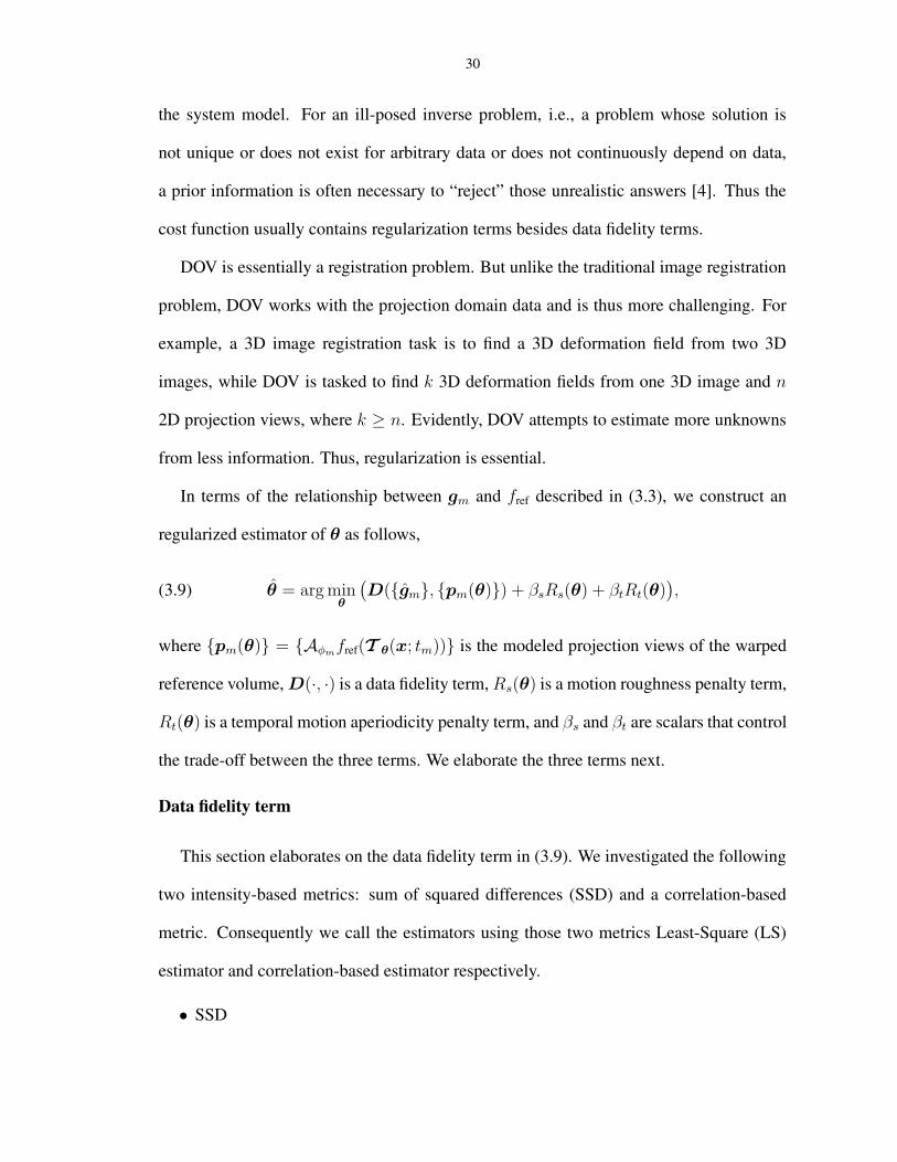
Data fidelity term
This section elaborates on the data fidelity term in (3.9). We investigated the following
two intensity-based metrics: sum of squared differences (SSD) and a correlation-based
metric. Consequently we call the estimators using those two metrics Least-Square (LS)
estimator and correlation-based estimator respectively.
• SSD
31
The expression of SSD is as follows,
(3.10) SSD({gm}, {pm(θ)}) =1
2MN
M∑
m=1
‖gm − pm(θ)‖2
where M is the number of projection views and N the number of detector elements of
the cone-beam scanner. This metric works well for registration of images from the same
modality. This rule applies to DOV as well. To yield good estimates using this approach,
the X-ray energies should be the same for imaging the static CT and for acquiring the
cone-beam projection views. In addition to this, extra effort may be needed to correct the
imaging artifacts such as Compton scatter effects, beam hardening effects, and presence
of the radiotherapy table in the projection views (not present in the prior CT). The SSD
represents “best case” performance when such effects are corrected. However, in practice
it may be difficult to correct for all such effects, so the following correlation-base metric
may be preferable.
• Correlation-based metric
In the correlation-based estimator, we used the negative-logarithm of the correlation coef-
ficient (LCC) as the data fidelity metric. The expression is as follows,
LCC({gm}, {pm(θ)})
=M∑
m=1
− ln(cor(gm,pm(θ)))
=M∑
m=1
(− ln
N∑
n=1
(gm,n − gm)(pm,n(θ) − pm(θ)) +
1
2ln
N∑
n=1
(gm,n − gm)2 +1
2ln
N∑
n=1
(pm,n(θ) − pm(θ))2),
(3.11)
where gm is the mean value of gm and pm(θ) is the mean value of pm(θ). In this data
fidelity term, we use a logarithm to separate the numerator and denominators in the expres-
sion of the correlation coefficient, which simplifies the calculation of its gradient. Because
32
the logarithm function is increasing, the logarithm step does not change the monotonic-
ity of the correlation coefficient function. We negate the logarithm correlation coefficient
because we are minimizing the cost function in the estimator (3.9).
Correlation-based metrics are suitable when the intensities of the images are linearly
related. In X-ray imaging, the attenuation is larger when the X-ray energy is stronger. So
we may expect the correlation-based estimator can perform well even if the energy spectra
used for the conventional CT scanner and the cone-beam CT scanner are not identical.
Penalty design
This section elaborates on the penalty terms in (3.9).
• Spatial and temporal motion roughness penalty
The motion roughness penalty discourages rapidly changing breathing motion estimates
that would be unrealistic. The spatial motion roughness can be measured qualitatively by
the squared differences between the displacements of adjacent voxels, and the temporal
motion roughness by the squared differences between the displacements of the same voxel
at adjacent time points. To simplify this term, we replaced the displacement differences
by the motion parameter differences. With this simplification, this term can be expressed
mathematically as
(3.12) R(θ) =1
2‖Cθ‖2 ,
where C is a differencing matrix, with a typical row having the form (. . . , 0,−1, 1, 0, . . .)
for the first-order roughness penalty and (. . . , 0,−1, 2, 1, 0, . . .) for the second-order rough-
ness penalty. It can be shown that the second-order differencing matrix has a very similar
high-pass structure to that for penalizing displacements under a cubic B-spline deforma-
tion model. By including this penalty term, the optimization is guided toward a solution
with a smoother breathing motion.
33
• Aperiodicity penalty
The aperiodicity penalty encourages similarity between deformation estimates that corre-
spond to similar respiratory phases. This helps ensure temporal regularity. If the temporal
knots are evenly spaced in each breathing period and each breathing period contains the
same number of knots, then the temporal deformation similarity can be quantified by the
closeness of the coefficient values of knots that are located at similar respiratory phases,
for the sake of simplicity. For example, in Fig. 3.12(solid line) there are four breathing
cycles, each containing 5 locally evenly spaced knots. Thus, every fifth knot corresponds
to a similar phase, such as the knot group (1, 6, 11, 16), the knot group (2, 7, 12, 17), and
so on. Based on this design, the aperiodicity penalty term also takes the form of Eq. (3.12),
with the matrix C having a typical row of (. . . , 0,−1, 0, . . . , 0, 1, 0, . . .). The number of
zeros between −1 and 1 is related to the number of knots placed in each breathing period.
To determine the correspondence between temporal deformations, we extract a respiratory
signal from the SI position change of the diaphragm in the projection views. Details of the
extraction method are given in Sect 3.2.
We add this penalty term to help overcome the limited gantry range for each breathing
cycle. Current radiotherapy systems can rotate 6◦ per second, spanning around 20−40◦ in
one breathing cycle. Therefore the measured projection views in one breathing cycle may
poorly reflect the motion along certain directions. For example, if the gantry starts from 0◦
(anterior view), then the projection views in the first breathing cycle are less informative
about the AP motion, leading to poorer motion estimation accuracy along the AP direction
in the absence of any other prior information. However, the projection views taken over
the next breathing cycle can better capture the motion along AP direction. By using an
aperiodicity penalty term, motion information contained in the adjacent breathing cycles
can be “shared” to help compensate for the angular limitation.
34
3.1.3 Optimization
we use iterative methods to search for θ. We experimented on several numerical algo-
rithms [62] and found that the Conjugate Gradient (CG) algorithm worked better the others
we experimented, such as the Gradient Descent (GD), the Levenberg-Marquadt(LM) and
Quasi-Newton (QN) algorithms. The GD algorithm chooses the search direction accord-
ing to the gradient vector, offering slow convergence and being easily stuck at a local
minima for DOV. The LM offered fast convergence for simulated small-size dataset, but
was impractical for 3D clinical data due to the computation of a large-sized Hessian. The
QN algorithm approximates the inverse of Hessian by updating a preconditioning matrix.
Based on our experiments, the approximation was not accurate enough to guide the opti-
mization toward a correct direction for this problem.
The CG algorithm does not use the gradient vector directly as its search direction. It
modifies the gradient search directions so that the current search direction is conjugate
to all the previous search directions. This modification ensures a more efficient search
over the parameter space and hence converges faster than the simple Gradient Descent
algorithm. The updating scheme for each iteration n includes the following steps,
q(n) = ∇ψ(θ(n)) (gradient)
p(n) = Pq(n) (precondition)
γn =
0, n = 0
real(〈p(n), q(n)−q(n−1)〉)
real(〈p(n−1), q(n−1)〉), n > 0
d(n) = −p(n) + γnd(n−1) (search direction)
αn = arg minα∈R
ψ(θ(n) + αd(n)) (stepsize)
θ(n+1) = θ(n) + αnd(n) (update).
(3.13)
35
We set P = I , which is actually the unpreconditioned case. Ideally the step size αn
should be solved exactly. However, convergence can also be guaranteed if αn satisfies the
Wolfe conditions []. To save computation time, we used only one iteration of the Newton
update to find a sub-optimal step size αn as follows,
(3.14) αn = α0 −ψ(α0)
ψ(α0),
where the initial value α0 is set to be zero to simplify the calculation. The proof is yet to
be done that such selected αn is within the range specified by the Wolfe conditions. The
gradient q(n), the first derivative ψ(α0) and the second derivative ψ(α0) can be found from
(3.9) using the chain rule. Refer to Appendix A for details of the calculation.
To accelerate the optimization procedure and to avoid local minima, we also applied a
multi-resolution technique [82].
3.2 Implementation issues3.2.1 Extraction of respiratory signal from projection views
As described in the Sect 3.1.2, We need a respiratory marker to determine the cor-
respondences between the temporal knots for the aperiodicity penalty. We adopted and
simplified the respiratory signal extraction method presented by Zijp’s [105]. The basic
idea is to capture the SI transition of the diaphragm in the collected projection views. The
method uses the following four steps:
Step 1: we applied a gradient filter (e.g., h = [−1, 1]) to each 2D projection image
along the Cranial-Caudal (CC) direction. This step is to emphasize the diaphragm-like
transition feature in each projection image (Fig. 3.2).
Step 2: We took the absolute value of each gradient image then projected onto the CC
axis (Fig. 3.3). The “image” formed by combining all the 1D projections clearly shows
some breathing pattern near the diaphragm region, while in the other regions there is no
36
(a) The X-ray pro-jection image
(b) Its CC gradientimage
Figure 3.2: The X-ray projection image (a) and its CC gradient image (b).
obvious intensity contrast (Fig. 3.4).
(a) The absolute value of thegradient image
(b) Its axial projection
Figure 3.3: The absolute value of the gradient image (a) and its axial projection (b).
Figure 3.4: The image formed by combining the 1D axial projections. Each column corresponds to a single1D projection.
Step 3: the centroid of each 1D projection was calculated and ordered in time. The
formula for calculating the centroid of a 1D signal sn, n = 1, · · · , N , is
centroid =
∑N
n=1 nsn∑N
n=1 sn
.
37
Step 4: the centroid signal was normalized and then smoothed by using a simple moving
average filter.
As shown in Fig. 3.12, the estimated respiratory signal (dashed line) presents similar
peak and valley patterns as that of the true respiratory signal (solid line). An advantage of
this projection-view based method is that the resulting signal is related to internal anatomy
positions, unlike external monitoring methods. We use this signal to decide the phase
correspondence between temporal knots for calculating the aperiodicity penalty term. This
is its only use here. Since this signal is not extremely important for the design of our
motion model, a rough estimation of the breathing signal is sufficient for DOV.
Figure 3.5: An illustration of the extracted breathing signal borrowed from our later simulation results. Thesolid line represents the true breathing signal and the dashed line represents the extracted breath-ing signal.
3.2.2 Use of Kronecker operator in B-spline related computations
Let us start from a 2D signal, f(x, y), represented by B-spline finctions as follows,
(3.15) f(x, y) =J∑
j
I∑
i
θij β
(x− xi
hx
)
β
(y − yj
hy
)
.
Suppose we want to calculate F , a discrete image of f(x, y) at positions {(xnx, yny
), nx =
1, · · · , Nx, ny = 1, · · · , Ny}. If we define Bx to be an Nx × I matrix with its element
38
Bx(nx, i having the following value
(3.16) Bx(nx, i) = β
(xnx
− xi
hx
)
,
and define By an Ny × J matrix similarly, the calculation of FNx×Nyis equal to the fol-
lowing linear operation,
(3.17) F = Bxyθs,
whereBxy = By ⊗ Bx, representing the B-spline matrix, and θs is the column-wise stack
of array θij Here ⊗ denotes the kronecker product.
In our case, we actually use a 4D B-spline tensor product as the basis function (3D
spatial and 1D temporal (x, y, z, t)), such as the calculation of deformation in Eq. (3.7).
The B-spline operator for this 4D case is
(3.18) Bxyzt = (Bt ⊗Bz ⊗By ⊗Bx).
The size of Bxyzt is (NxNyNzNt) × Nθ, where Nx, Ny, Nz and Nt are the number of
positions where the values of the function are required to be calculated along the four
dimension respectively and Nθ is the total number of B-spline knots. Directly forming
the matrix Bxyzt and then multiplying with the coefficient vector θs may require huge
computation memory. To overcome possible memory problem, we utilize the following
property of the kronecker product:
When dimensions are appropriate defined for the product ABC to be well defined,
(3.19) (ABC)s = (C ′ ⊗ A)Bs.
Hence the large matrix multiplication can be decomposed into many small matrix multi-
plications and it is not neccessary to store the large B matrix.
39
3.3 Simulation
This section presents our simulation results. The simulated datasets were generated
based on several real clinical planning CTs and the geometry of a slowly rotating cone
beam CT system, and thus should reflect sufficiently realistic conditions to illustrate the
performance of this method. Furthermore, in the simulations absolute truth is known,
permitting quantitative evaluation.
3.3.1 Simulation setupData setup
This section describes how we generated sequential cone-beam projection views of a
moving CT volume using three breathhold treatment CT volumes of the same patient at
We selected the thorax CT at the end of exhale (0%) as our reference volume (Fig. 3.6),
with 192 × 160 × 60 voxels and a voxel size of 2 × 2 × 5mm3. We then generated 70
cone-beam projection views of the warped reference volumes over a 180◦ rotation. (The
warping process is described in the next paragraph.) The simulated cone-beam system had
a flat-panel detector of 180 × 200 elements of size 4 × 4mm2. The source to isocenter
distance and the isocenter to detector distance were 1000mm and 500mm respectively.
The gantry rotated 6◦ per second and spanned 180◦ over the four breathing cycles. We
used a distance-driven method [14] to calculate the projection views. To simulate realistic
projection views, scatter and Poisson noise were added according to the statistical property
of projection views as described in (3.4). We first converted the projection views from
attenuation to primary photon counts. The incident intensity Im,n in (3.4) used for this
conversion is 106 counts per ray [93]. We then applied a convolution method to generate
the scatter counts, in which a normalized 2D exponential kernel with a FWHM of 4cm [47]
40
and a scatter to primary ratio (SPR) of 10% was convolved with the primary photon counts.
In practice the SPR may be higher. Finally the scatter counts and the primary counts
were added together and their sums were treated as parameters of the MATLAB function
“poissrnd” to generate Poisson distributed noisy projection views. Fig. 3.7 displays several
simulated cone-beam projection views.
(a) Axial view (b) Coronal view (c) Sagittal view
Figure 3.6: The three views of the reference thorax CT volume. (Points in the images are the projectionpositions on the three planes of the voxels randomly selected for accuracy plots .
(a) 28◦ (b) 70
◦ (c) 112◦ (d) 154
◦
Figure 3.7: Examples of simulated motion-included cone-beam projection views. From left to right, theprojection angles are 28◦, 70◦, 112◦, 154◦.
The respiratory motion we simulated for generating the dynamic cone-beam projection
views was based on the three breathhold CT volumes (0%, 20%, 60% vital capacity).
We first registered the 20% and 60% volumes to the 0% volume using a B-spline based
deformation model. Then we selected some voxels near nonuniform regions such as the
top surface of diaphragm and the intersections of bronchi, which have smaller registration
41
errors. Afterward, we found the time points t20 and t60 corresponding to the 20% and 60%
tidal volumes that best fit the SI displacement of the selected voxels into the following 1D
temporal motion model (3.20) [52],
(3.20) z(t) = z0 − a cos6(πt/τ − π/2),
where z0 is the SI position at exhale, a is the amplitude of the motion. Knowing the de-
formations at three time points and with the symmetry assumption between the motions
of exhalation and inhalation, we performed temporal interpolation (separable for each of
three directions) of the deformations at each voxel using the MATLAB function “csape”
to form one cycle of temporally continuous breathing motion. Four breathing cycles with
a total 30-seconds duration were simulated, each with different breathing periods and am-
plitudes. The solid line in Fig. 3.12 shows the simulated respiratory signal.
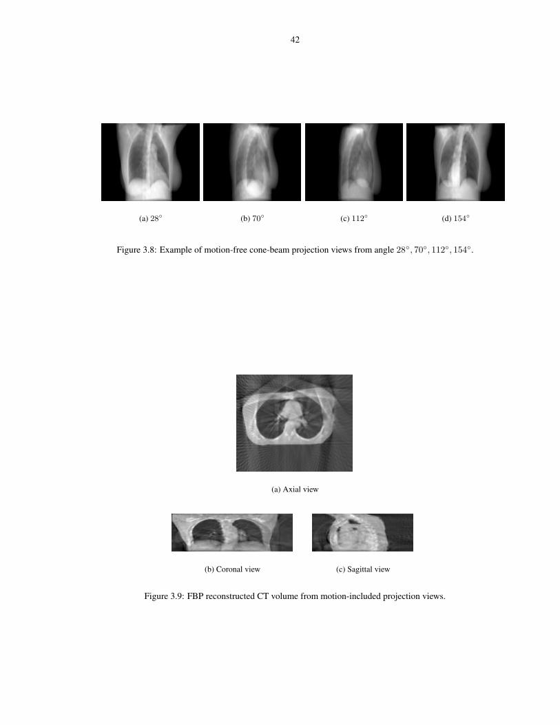
To illustrate the motion artifact in the direct reconstruction, we applied FBP method to
the simulated motion-included projection views and compared the reconstructed volume
with that reconstructed from motion-free projection views (generated using the same ref-
erence volume under the same cone-beam geometry but without motion) (Fig. 3.8). The
reconstructed CT volumes from motion-included and motion-free projection views are
displayed in Fig. 3.9 and Fig. 3.10 respectively. It is obvious that the images in Fig. 3.9
present many blurring artifacts at the internal lung structures and the edge of the chest wall
and diaphragm region because of the inconsistent projection views caused by respiratory
motion. Since our goal is to estimate respiratory motion rather than image reconstruction,
we are not concerned about the streak artifacts present in both reconstructed volumes due
to the small number of projection views.
Preparation for DOV
• Data preprocessing
42
(a) 28◦ (b) 70
◦ (c) 112◦ (d) 154
◦
Figure 3.8: Example of motion-free cone-beam projection views from angle 28◦, 70◦, 112◦, 154◦.
(a) Axial view
(b) Coronal view (c) Sagittal view
Figure 3.9: FBP reconstructed CT volume from motion-included projection views.
43
(a) Axial view
(b) Coronal view (c) Sagittal view
Figure 3.10: FBP reconstructed CT volume from motion-free projection views.
This step obtains the projection views {gm} from the measured photon counts using (3.5).
We used a simple scatter estimate that was obtained by convolving the noisy photon counts
with the same exponential kernel used for generating the scatter. For real cone-beam pro-
jection views, the scatter estimation should be more complex. In simulation we deliber-
ately used a simple scatter correction method so the scatter was incompletely corrected, as
is the case in practice.
• B-spline knot distribution
The placement of B-spline control knots can be very flexible. It can be either a uniform
distribution, or a nonuniform distribution. Theoretically, finer control grids enable more
accurate approximation of a continuous signal. But in practice, due to the presence of
noise, very fine control grids may overfit the noise. Furthermore, a finer control grid assi-
ciates with more parameters, complicating optimization. One can adjust the knot spacings
manually, starting with a relatively coarse control grid, and then decreasing the knot spac-
ings until the optimizations with the two most recent control grids reaches very similar
44
results.
For our estimation, the sptial control knots were spaced evenly in the thorax region,
with spacings of hx = 16voxels, hy = 16voxels, hz = 10voxels along the LR, AP
and SI direction respectively.. They were placed differently from the knot locations used
for simulating the motion and with less density. For the temporal knot placement, we
used non-uniform distribution. We evenly placed 5 knots in each active breathing period,
yielding 20 temporal knots along the entire temporal axis. The active breathing period is
defined to be the interval from start-inhalation to end-exhalation. A short rest interval fol-
lows each active breathing interval. Because the deformation during a rest interval would
be very small with respect to the reference volume, which is assumed corresponding to
end-exhalation state. We did not place any temporal knots in this interval, reducing the
number of parameters to be estimated. This nonuniform temporal knot placement facil-
itates establishment of the phase correspondence between knots for aperiodicity penalty
design, as described in Sect 3.1.2. See Fig. 3.11 for an illustration of this knot placement.
0 5 10 15−0.2
0
0.2
0.4
0.6
0.8
1
1.2
t(sec)
breathing signaltemporal knot distribution
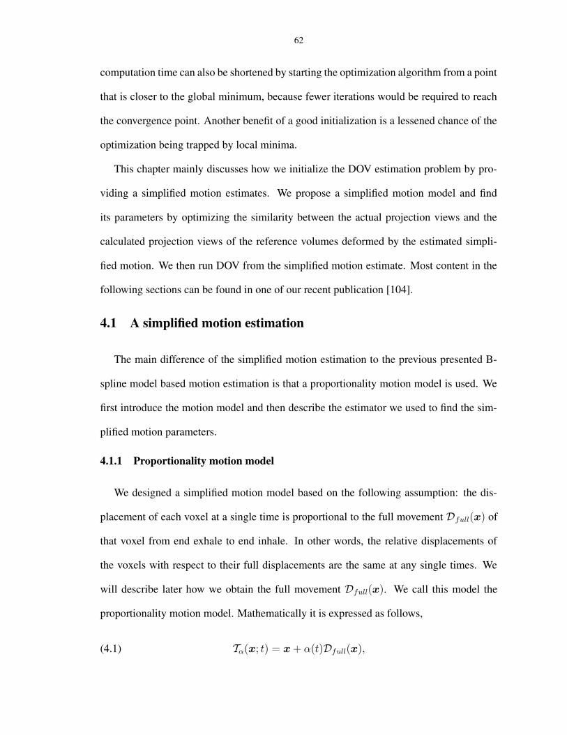
Figure 3.11: Illustration of an ideal temporal knot placement assuming respiratory signal known
• Optimization setup
45
For optimization, the motion parameters were all initialized to be zero. We terminated the
optimization algorithm when the absolute difference of the cost function value between the
two most current iterations was less than a threshold. We also applied a multi-resolution
technique to accelerate the optimization procedure and to avoid local minima. We started
the optimization from a downsampled-by-2 version of both the reference volume and the
projection views, then used the coarser-scale result as an initialization for the next finer-
scale optimization. It took about 65 iterations at the coarser level and 45 iterations at the
finer level to converge. The total computation time was about 10 hours using Matlab on a
3.4GHz Pentium computer.
3.3.2 Results and discussion
In this section we studied the effects of the temporal knot distribution, the aperiodic-
ity penalty and the two similarity metrics on the DOV performance. We quantify DOV
estimation accuracy using the means and standard deviations of the differences between
the estimated and the true simulated displacements of the voxels over the entire volume
through all time points.
Effects of the temporal knot placement
We present two cases of results using the penalized LS estimator. One case uses an ideal
temporal knot placement (“*” signs in Fig. 3.12), based on the true respiratory signal. The
other case was with automatic temporal knot placement (“+” signs in Fig. 3.12) according
to the estimated respiratory signal from projection views. In the former case, since the
true respiratory signal was used, the phase correspondences among the knots in adjacent
breathing cycles were exact and thus the periodicity regularity term could accurately align
the the deformations at the same phases. The ideal case offers us a guideline on how well
this proposed algorithm would perform. In the latter case, the peak intervals were detected
46
automatically from the estimated breathing signal and temporal knots were spaced evenly
in each peak intervals. Because of the mismatch between the estimated and true respiratory
signals, offsets existed between the phases of the knots that were assumed to fall into the
same breathing phases by the aperiodicity penalty term. This represents a practical case,
where the ground truth of the respiratory signal is unavailable.
Some large deformation errors did occur, even in the case of ideal temporal knot place-
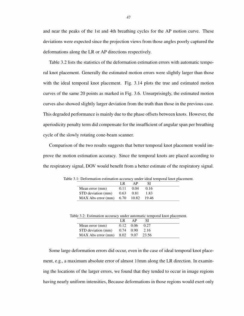
ment, e.g., a maximum absolute error of almost 10mm along the LR direction. In examin-
ing the locations of the larger errors, we found that they tended to occur in image regions
having nearly uniform intensities, Because deformations in those regions would exert only
48
0 5 10 15 20 25 30−20
−15
−10
−5
0
5
10
t (sec)
Disp
lace
men
t (m
m)
True APTrue LRTrue SIEstimated APEstimated LREstimated SI
Figure 3.13: Accuracy plot of the randomly selected 20 points under the optimization with ideal temporalknot placement. The thick lines represent the true motion curves averaged over the 20 points.The thin lines represent the estimated motion curves averaged over the 20 points. Error bars onthe thin lines represent the standard deviations of the deformation estimation errors.
49
0 5 10 15 20 25 30−20
−15
−10
−5
0
5
10
t (sec)
Disp
lace
men
t (m
m)
True APTrue LRTrue SIEstimated APEstimated LREstimated SI
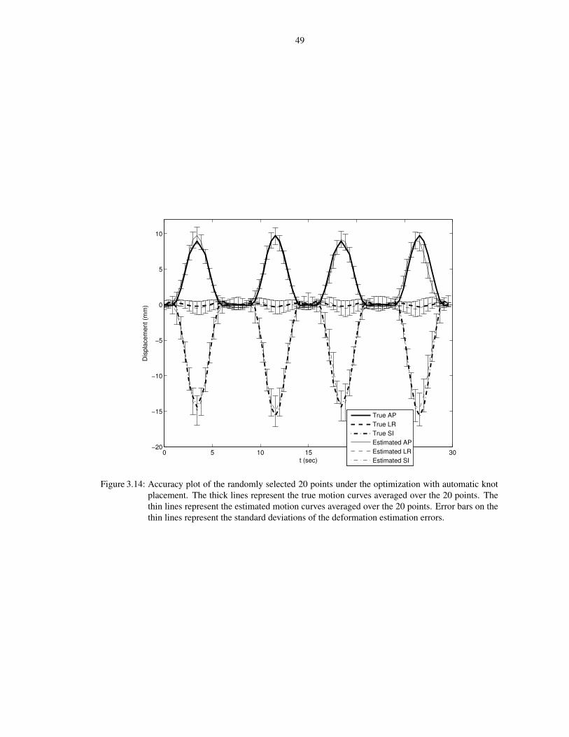
Figure 3.14: Accuracy plot of the randomly selected 20 points under the optimization with automatic knotplacement. The thick lines represent the true motion curves averaged over the 20 points. Thethin lines represent the estimated motion curves averaged over the 20 points. Error bars on thethin lines represent the standard deviations of the deformation estimation errors.
50
very slight changes on the projection views. So these errors are likely due to a lack of
image structures, which is common for registration problems.
A second possible source of error is motion model mismatch, i.e., the respiratory mo-
tion could not be recovered fully by the B-spline motion model with the designed control
grid. We did B-spline least square fitting of the synthetic motion using the same control
grid to examine how much error would result from the model mismatch alone. Table 3.3
gives the statistics of the B-spline approximation errors. Overall the approximation er-
rors were very small, but there were also some relatively large errors. We examined the
location where the largest AP motion fitting error occurred to see how well the DOV esti-
mation performed at that voxel. Fig. 3.15 compares the estimated and the fitted AP motion
curves of that voxel. These two curves are close to each other, indicating that the estimated
motion was close to the optimum under the selected motion model at this voxel, which did
happen to be in a nonuniform region.
Table 3.3: B-spline least squares fitting error under ideal temporal knot placement.LR AP SI
The aperiodicity penalty is necessary for DOV because of the limited gantry angles in
one breathing cycle. A too small βt may not sufficiently bring the motion information
from the adjacent breathing cycles to compensate this limitation, while a too large βt may
subdue the role of the local motion information. This is a tradeoff. To study the impact
of this term, we ran DOV using the penalized LS estimator with different βt values and
plotted the estimation accuracy in Fig. 3.16. As βt increases from 10−6, the mean errors
and the standard deviations in each direction tend to drop and then rise again after βt is
51
0 5 10 15 20 25 30−5
0
5
10
15
20
25
30
t(sec)
Disp
lace
men
t(mm
)
TrueB−spline FittedEstimated
Figure 3.15: AP motion curves of the voxel where the maximum B-spline fitting error along AP directionoccurs: the true (solid line), the B-spline fitted (dashed line) and the estimated by DOV (dasheddot line).
larger than 10−4. In realistic we may adjust this value by examining the regularity of the
breathing signal.
−8 −6 −4 −2
−2
0
2
4LR
log10(βt)
Mea
n er
ror (
mm
)
−8 −6 −4 −2
−2
0
2
4AP
log10(βt)
Mea
n er
ror (
mm
)
−8 −6 −4 −2
−2
0
2
4SI
log10(βt)
Mea
n er
ror (
mm
)
Figure 3.16: The mean errors and standard deviations v.s. the aperiodicity penalty parameter βt
The penalized LS and the correlation-based estimator
Table 3.4 compares the estimation accuracies of the penalized LS and the correlation-
based estimator. As can be seen from the table, the two estimators perform comparably
when the intensity of the modelled projection views matches those of the measured views.
Fig. 3.17 draws the accuracy plot of the 20 points using the correlation-based estimator.
This plot also resembles the accuracy plot of the penalized LS estimator in Fig. 3.14.
52
Table 3.4: The estimation accuracy of the LS estimator and the correlation-based estimator. The mean errorsand the standard deviations were calculated over the whole volume through time
True APTrue LRTrue SIEstimated APEstimated LREstimated SI
Figure 3.17: Accuracy plot of the randomly selected 20 points using the correlation-based estimator withideal temporal knot placement. The Thick lines represents the true motion curves averagedover the 20 points. The thin lines represents the estimated motion curves averaged over the20 points. Error bars on the thin lines represent the standard deviations of the deformationestimation errors.
53
3.4 Phantom experiment
We realize that the realistic condition would be more complex than what can be simu-
lated purely by computer, for example, the noise in the acquired data contains both Poisson
and Gaussian, the residual scatter effect after correction may still be prominent. Therefore
we conducted a phantom experiment that is more realistic to further test the DOV perfor-
mance.
3.4.1 Phantom and data collection
We used a partially deformable thorax phantom to test the performance of DOV, shown
in Fig. 3.18. It is composed of a rigid frame and a compressible foam compartment inside,
with some balls inserted. A rigid, flat plastic board is placed at the bottom of the phantom
to simulate a diaphragm. This “diaphragm” is connected to a linear actuator through a
piece of wood. Driven by the actuator, the “diaphragm” can move back and forth to com-
press and deform the material inside. The motion pattern of the “diaphragm” is controlled
by the actuator. For this experiment, we used a motion profile with alternating amplitudes
of 20 mm and 15 mm and alternating periods of 9 s and 6 s (Fig. 3.19).
We first scanned the phantom using a conventional CT. The voltage of the X-ray tube
for this CT was set to 120kv. We scanned the phantom in three motion states, with the
“diaphragm” positioned at 0cm, 1cm and 2cm toward the neck. We named the three static
volumes to be CT0, CT1 and CT2 respectively. The reconstructed volumes have a size of
512×512×89 with the voxel size of 0.98×0.98×3 mm3. CT2 was used as the reference
volume for DOV. The other two were used as a measure of truth to evaluate the estimation
accuracy of DOV.
Then we moved the phantom to a slowly rotating cone-beam system and started the
actuator and took a 360◦ scan of the moving phantom. Manual laser alignment was per-
54
Figure 3.18: A picture of the movable phantom: 1. the phantom; 2. the diaphragm; 3. the wood connector;4. the actuator.
0 5 10 15 20 25 30−25
−20
−15
−10
−5
0
t (sec)
The
diap
hrag
m S
I disp
lace
men
t of t
he p
hant
om (m
m)
The motion profile
Figure 3.19: The motion profile created for the actuator.
55
formed to set up the phantom right before starting the cone-beam scan. But instead of
placing the phantom at the correct setup position, we deliberately moved the phantom off
about 1 cm along the axial direction to test DOV with setup errors. After completing the
cone-beam scan of the phantom, we removed the phantom and collected a full cone-beam
scan of the table. The table scan was used to normalize the measured photon counts of the
phantom scan. For the cone-beam scanner, the voltage of the X-ray tube was set to 125kv.
The distance from the X-ray source to the detector was 1500.0mm and to the isocenter was
1000.0mm. The size of the 2D flat-panel detector was 397 × 298mm2. The gantry rotated
at 6◦ per second with a frame rate of about 11fps. Totally 668 views were collected for a
full rotation.
3.4.2 Preprocessing
We cropped the reference CT and downsampled it by 2 in the axial plane. After crop-
ping and downsampling, the size of the reference CT was 192 × 180 × 89 and the voxel
size was 2.0 × 2.0 × 3mm3. Fig. 3.20 shows three views of the CT volume. The intensity
of the measured projections from the CBCT scanner are linear to the photon counts. We
needed to convert the counts to attenuation. The conversion was done by taking logarithm
of the table scan divided by the phantom scan, i.e.,
(3.21) attenuation = lnthe table scan
the phantom scan
An advantage of using the table scan rather than an air scan as a normalization factor
is that the table artifact may be greatly removed from the phantom scan. However, the
table artifact can not be totally removed, (as can be seen in Fig. 3.21), because the scatter
and beam-hardening effects were different in the table scan and phantom scan. For the
purpose of DOV, we only used the views in the first 180◦ interval and downsampled them
by 4 in the temporal axis, so there were about 80 views spanned over 180◦ used by DOV.
56
The projection views were truncated views since the 2D detector was not large enough
to cover the whole width of phantom. We also downsampled each projection views by 4.
After this spatial downsampling, the size of each projection view was 252 × 188 and the
pixel resolution was 1.6mm × 1.6mm.
Before running DOV, we estimated the setup difference between the conventional CT
and the cone-beam CT system. Without setup correction, the estimated motion by DOV
would compensate for the setup errors which do not belong to the real organ motion caused
by breathing. Usually a rigid setup difference is assumed. It can be described by six pa-
rameters {φx, φy, φz, tx, ty, tz}: three rotation angles and three translations along each
axis respectively. These parameters can be estimated by aligning the computed projection
views of the reference volume to a few measured projection views. This method belong to
the field of 2D-3D registration which is commonly used for setup correction in radiother-
apy [37, 60, 90]. Usually the projection views used in those registrations do not include
organ motion. However, this is not the case for the collected projection views in DOV.
To meet the consistency requirement, the setup difference estimation used several projec-
tion views approximately corresponding to the motion phase of the reference volume. The
correspondence can be established based on the extracted breathing signal from the di-
aphragm transition. Correlation-based metric was used in the registration. The estimated
setup difference was {0.0001rad, 0.0038rad, 0.0061rad, 0.89mm, −0.02mm, 7.74mm}.
Although the estimation accuracy is expected to be improved further, the phantom ex-
periment did illustrate the feasibility of the DOV principle, because this experiment re-
flected the realistic situations in the following three points of view. First, the movable
phantom imitated a real human thorax. Second, a slowly rotating cone-beam CT scanner
integrated in a radiotherapy simulator was used to collect the projection views, in which
real imaging artifacts existed such as the truncated views, the presence of radiotherapy
table, Compton scatter and beam-hardening effects. Third, setup differences between the
conventional CT scanner and the cone-beam CT scanner were also considered.
However, the motion pattern of the phantom we created may be simplified compared
to the true breathing motion, which would be much more irregular in both amplitude and
period. This irregularity may bring uncertainty in selecting the aperiodicity penalty pa-
rameter βt. In our phantom experiment, βt was set to be 10−4, the value that yielded the
best estimation in the simulation, because the motion patterns of the phantom and the sim-
59
ulation were similar. In a real patient study, a monitor may be used to instruct patients to
breathe in a more regular way to reduce the difficulty in selecting βt.
Although the phantom motion pattern was simple, the spatial deformations of the phan-
tom included intensive “sliding” between the edge of the “diaphragm” and the interior side
of the body frame. This kind of deformation is challenging to fit by the pure B-spline
model. In real patients, this “sliding” phenomenon would be somewhat reduced. There-
fore we may expect better estimation accuracy in a real patient case.
Due to a large angle of the X-ray cone and the use of a 2D detector, substantial scatter
effects were present in the collected cone-beam projection views. In our current phantom
experiment, a posterio scatter correction was skipped. This step will be implemented in the
near future. We can build a beam stop array to obtain a scatter estimate. A beam stop array
consists of small lead disks pressed into holes in an acrylic sheet. It can be placed right
after the X-ray source collimator so the projection image reflects the scatter distribution at
the positions where the lead disks are projected at, providing an estimate of the scatter [57].
These scatter images are acquired separately from the respiration correlated cone-beam
projection views. We believe including a scatter correction can further improve the DOV
accuracy.
The estimated deformation errors for the phantom experiment were largely around the
resolution of one voxel. Smaller errors can be expected using a reference volume with a
higher resolution. In this experiment, we started the estimation with the downsampled-
by-4 reference volume and projection views, and stopped it at the level of downsampled-
by-2 resolution. Increase to the resolution of the oringinally acquired data will require
intensively great computation time. We realize that the long computation time will limit
the usage of the DOV method in clinic. The bottleneck of the computation is evaluating
(3.3) and (3.2), the 3D deformed reference volumes and their projection views at each
60
time points. Since most of the computation can be implemented separately view by view,
the computation time can be reduced by parallel computing with a multi-processor CPU.
Another possible way to reduce computation time is to accelerate the convergence of the
optimization algorithm. We will discuss this possibility in the next section.
CHAPTER 4
Acceleration of DOV
We have shown in the previous chapter that the internal motion of patients during
breathing can be estimated from a sequence of slowly rotating 2D cone-beam X-ray pro-
jection views and a static prior of of the patient’s anatomy. The so-called DOV method
yielded encouraging results, with the RMS errors around the voxel size both in the simu-
lation and the phantom experiment. However, we have realized that the computation time
was very long. It involves heavy-loaded operations on data sets with very large size, such
as the warping and forward projection of 3D volumes, plus a huge number of parameters
associated with motion model to be optimized. For example, for the data presented in the
phantom experiment, it took about 10min for each iteration and the optimization process
converged at about the 50th iteration. The long computation may limit the usage of DOV
in clinic.
There are several ways to accelerate this whole estimation procedure. One way is
to use multi-processor CPU and do parallel computing. Since the deformations of the
reference volume and the projections of the deformed reference volume can be computed
separately view by view, using a N-processor CPU may reduce the whole computation time
by a factor of close to N. One may also utilize a graphics accelerator card to reduce the
time for projection operators. Other than those acceleration methods through hardwares,
61
62
computation time can also be shortened by starting the optimization algorithm from a point
that is closer to the global minimum, because fewer iterations would be required to reach
the convergence point. Another benefit of a good initialization is a lessened chance of the
optimization being trapped by local minima.
This chapter mainly discusses how we initialize the DOV estimation problem by pro-
viding a simplified motion estimates. We propose a simplified motion model and find
its parameters by optimizing the similarity between the actual projection views and the
calculated projection views of the reference volumes deformed by the estimated simpli-
fied motion. We then run DOV from the simplified motion estimate. Most content in the
following sections can be found in one of our recent publication [104].
4.1 A simplified motion estimation
The main difference of the simplified motion estimation to the previous presented B-
spline model based motion estimation is that a proportionality motion model is used. We
first introduce the motion model and then describe the estimator we used to find the sim-
plified motion parameters.
4.1.1 Proportionality motion model
We designed a simplified motion model based on the following assumption: the dis-
placement of each voxel at a single time is proportional to the full movement Dfull(x) of
that voxel from end exhale to end inhale. In other words, the relative displacements of
the voxels with respect to their full displacements are the same at any single times. We
will describe later how we obtain the full movement Dfull(x). We call this model the
proportionality motion model. Mathematically it is expressed as follows,
(4.1) Tα(x; t) = x + α(t)Dfull(x),
63
where α(t) represents a 1D proportionality motion signal.
The simplified motion model (4.1) is also built upon a prior of the full deformation
of the patient during inhale, Dfull(x). We estimate it by registering two reference CT
volumes of the patient, one at end exhale and one at end inhale, denoted fex(x) and fin(x)
(x ∈ R3) respectively. Usually these two reference volumes are clinically available for
treatment plan. Again we used a B-spline based deformation model for registration, It
finds the deformation parameters for Dfull(x) by minimizing a cost function containing a
SSD similarity term and a Jacobian penalty term [36], as described in Sect 2.1.4. SSD can
be used as the similarity measure for this registration problem because the two reference
volumes are with the same imaging modality.
4.1.2 The simplified motion estimator
For simplicity, in the results shown below, we parameterize the continuous proportion-
ality function α(t) using its discrete samples α = {αtm},m = 1, · · · ,M through a Rect
basis function as follows,
(4.2) α(t) =M∑
m=1
αtmRect(t− tmTp
),
where Tp is the time interval between adjacent projection view acquisitions. Alternatively,
smooth basis may work finer. With the above representation of α(t), the goal for the sim-
plified motion estimation is to find {αtm},m = 1, · · · ,M , the sampling points of α(t)
at the projection acquisition times. We estimate these parameters by optimizing the sim-
ilarity between the measured projection views and the calculated projection views of the
deformed reference volumes by the proportionality motion model as follows, The formula
of this estimator is as follows,
(4.3) α = arg minα
(
LCC({gm}, {Aφm
fref (Tα(x; tm))})
+ λR(α)
)
,
64
Similarly to (3.9), LCC(·, ·) is the data fidelity term measuring the correlation coefficient,
as expressed in (3.11). R(·) is a roughness penalty term, taking the form of 1/2||Cα||2,
where C is a differencing matrix.
The simplified motion estimator does not contain an aperiodicity penalty term. This
term can be omitted because the problem posed by the limited angular range over one
breathing cycle is compensated by some property of the proportionality motion model.
This property is that this model restricts the relative displacements along the three direc-
tions of each voxel with respect to its full displacements are the same. This restriction
interconnects the motion along each direction, dislike the B-spline motion model, which
treats the motion along each direction independently.
We again use the CG algorithm to solve (4.3). Because of the smaller number of pa-
rameters associated with the proportionality motion model, a downsampled reference vol-
ume and projection views may already be sufficient for this estimation problem. As will
be shown later in Table 4.1, the estimation accuracies are very similar when using the
datasets with and without downsampling-by-2. Hence we can solve this problem using
datasets with smaller sizes, reducing the computation time.
The simplified motion estimate can be used twofold. First, it can be treated as an
initialization for DOV with B-spline motion model, which is the main purpose for this
part of work. Second, the 1D sequence α represents the averaged relative deformation
over time with respect to the full deformation. It can be used as a breathing signal to
guide the temporal knot placement. As will be shown in the simulation, the estimated
1D sequence α would be more closer to the true breathing pattern than the one extracted
from measured projection views. Therefore, α can guide us to place the temporal knots
so that the phase correspondences between knots in the apriodicity penalty term are more
accurate.
65
4.2 LS fitting of the simplified motion estimate into B-spline motionmodel
The simplified motion estimate αDfull(x) offers an initial guess of the motion. We
then implement a least-square fitting of αDfull(x) into the B-spline motion model (5.2),
to obtain an initial set of B-spline knot coefficients θ0. The optimization for DOV with a
B-spline model will then start from θ0.
Least-square fitting can be done analytically. Because the B-spline deformation model
is used in our registration to obtain Dfull(x), we only need to fit α into a B-spline function,
i.e., find ρ such that,
(4.4) α(t) =J∑
j=1
ρj β
(t− τj
∆t
)
holds at every time sample index tm. As described in Sect 3.2, Eq. (4.4) holds at discrete
time indices can be expressed as,
(4.5) α = Btρ,
where Bt is an M × J matrix with entry Bt[m, j] = β(
tm−τj
∆t
)
. Then the solution of (4.5)
can be found by takeing the adjoint operator as follows,
(4.6) ρ = (B′tBt)
−1B′tα,
Assume
(4.7) Dfull(x) =I∑
i
γi β
(x − xi
∆x
)
,
where {γi} are the B-spline knot coefficients of the full deformation map which we have
already estimated from registration, then we obtain the initial values of the B-spline motion
by taking the following Kronecker operation,
(4.8) θ0 = ρ ⊗ γ.
θ0 is then is input to the DOV optimization algorithm to enable faster convergence.
66
4.3 Computation complexity
The implementation of both motion estimators (3.9) and (4.3) includes the following
operators on 3D volumes: B-spline based image interpolation, B-spline based image de-
formation, and cone-beam forward projection. The computation complexity for the opti-
mization algorithm is approximately in the order of O(CMV U), where C is the number
of motion parameters, M is the number of projection views, V is the size of the static
reference volume and U is the size of each projection views.
For the B-spline motion model, the number of knots we used in simulation and phantom
experiment are in the order of 105; while for the proportionality motion model, the number
of parameters was equal the number of projection views, which was less than 100 in both
simulations and the phantom experiment. Furthermore, because of the small number of
parameters, we can estimate the the proportionality motion parameters using downsam-
pled reference volume and projection views. so the computation of the simplified motion
estimator is significantly shorter than DOV with B-spline motion model.
4.4 Performance evaluation
We tested this acceleration method on the simulated and phantom data sets. We com-
pared the performance of the following three DOV estimators:
• DOV with “zero” initialization: DOV starting from a coarser resolution with all pa-
rameters initialized to be zeros.
• DOV with initialization: DOV from the simplified motion estimates.
• Simplified motion estimator
We need one more reference volume for the simplified motion estimator. For the simu-
lation case, we added the 60% breath-hold CT volume. For the phantom case, we added
67
CT0, which corresponding to a 0cm movement of the diaphragm.
4.4.1 Simulation
We first registered the 0% and the 60% CTs to obtain the full deformation. We then
downsampled the exhale reference volume in the transaxial plane and each projection view
by 2 and executed the simplified motion estimator. The optimization converged at about
the 20th iteration, with each iteration taking about 30sec. Since the simple proportionality
motion model contained a small number of degrees of freedom, using the downsampled
images would not degrade the accuracy of the simple motion estimates but would greatly
reduce the computation time. This conjecture agrees with the results presented in Table
4.1. Fig. 4.1 shows the estimated motion proportionality parameters (dash line). It resem-
bles the “true” breathing pattern very closely. So, for DOV with B-spline motion model,
we can place the temporal knots according to the estimated signal α. Such placement is
closer to the ideal temporal knot placement than that according to the extracted breathing
signal, helping increase the estimation accuracy as discussed in Sect 3.3. Starting from
the simplified motion estimate, DOV converged with considerably fewer iterations almost
half of iteration number of DOV with “zero” initialization, as seen in the convergence plot
Fig. 4.2. Table 4.2 list the estimation accuracy of the three estimators. DOV with initial-
ization achieved similar accuracy to that of DOV with “zero” initialization, but with only
half of the latter’s computation time.
Mean error/ STD (mm) LR AP SIDownsampled by 2 -0.05/0.19 0.03/0.37 -0.09/0.88W/O downsampling -0.05/0.18 0.03/0.35 -0.09/0.84
Table 4.1: Estimation accuracy for the simple motion estimation on the simulation data. The table shows themean and the standard deviation (STD) of the errors over the entire volume through time. Theestimation accuracy with data downsampled by 2 and without data downsampling attained verysimilar performance.
68
Mean error/ STD (mm) LR AP SIDOV with “zero” initialization 0.12/0.74 0.06/0.90 0.27/2.16DOV with initialization -0.02/0.22 0.04/0.43 -0.03/0.90Simplified motion estimator -0.05/0.19 0.03/0.37 -0.09/0.88
Table 4.2: Estimation accuracy of DOV with “zero” initialization and DOV starting from simplified motionestimates
0 5 10 15 20 25 30−0.2
0
0.2
0.4
0.6
0.8
1
t (sec)
Brea
thin
g sig
nal
"True" breathing signalEstimated αExtracted breathing signal
Figure 4.1: The estimated motion proportionality parameters α.
4.4.2 Phantom experiment
We also tested the simple motion estimation on the phantom data set. Readers may
refer to Sect 3.4 for the detail on the experiment setup and data collection.
Fig. 4.3 plots the estimated proportionality parameters α and the motion profile of
the actuator that drove the movement of the phantom. As can be seen, the estimated α
resembles the actual motion profile very closely. Again, by initializing with the simpli-
fied motion estimates, DOV achieved faster convergence. The estimation accuracy of the
simplified motion estimates and the motion estimates of the two DOV cases are listed in
Table 4.3. As can be seen in the this table, DOV starting from simplified motion estimates
improved the estimation accuracy in the LR and AP directions, comparing to those with
“zero” initialization. Table 4.3 also indicates that DOV with initialization resulted in larger
estimation errors than the simplified motion estimator itself. This phenomenon may be
69
0 5 10 15 20 25 30 35 40 450
0.2
0.4
0.6
0.8
1
1.2x 10⁻³
Iteration number
Cost
func
tion
valu
e
DOV with "zero" initializationDOV starting from simplified motion estimates
Figure 4.2: Convergence curves of the DOV with “zero” initialization and DOV starting from simplifiedmotion estimates
explained as follows. The collected projection views contained severe scatter effects and
table artifact, as seen in Fig. 3.21. The estimator treated the useful data information and
those artifacts equally. Although the more complex B-spline motion model could charac-
terize local deformations better, it might overfit the noise artifacts on the other hand. In ad-
dition,the actual phantom motion may agree with the motion proportionality assumption.
Thus the estimator with the simplified motion model could find closer-to-truth solutions,
while the one with B-spline motion model performed worse. This phenomenon suggests
that a posterior scatter correction may improve the DOV motion estimation accuracy.
Mean error/ STD(mm) LR AP SISimplified motion estimator -0.02/0.06 0.01/0.07 0.47/0.38DOV with “zero” initialization 0.42/2.49 1.08/2.24 0.24/1.72DOV starting from simplified motion estimates 0.41/0.68 1.03/0.91 -0.04/2.19
Table 4.3: Estimation accuracy of the simplified motion estimator, DOV with “zero” initialization and DOVstarting from simplified motion estimates. The table shows the mean and the STD of the errorsover the landmarks.
70
0 10 20 30−25
−20
−15
−10
−5
0
t (sec)The
diap
hrag
m S
I disp
lace
men
t of t
he p
hant
om (m
m)
The motion profile
0 20 40 60 80−0.2
0
0.2
0.4
0.6
0.8
1
1.2
t (sec)
The estimated proportionality motion parameters α
Figure 4.3: The motion profile and our estimated scalar motion proportionality parameters α. The estimatesresemble the pattern of the motion profile.
4.5 Summary on DOV
In chapter 3 and 4 we described DOV, a method to estimate respiratory motion from a
sequence of slowly rotating X-ray cone-beam projection views. In this method, we adopt
a B-spline motion model, deform a breathhold thorax CT volume according to the motion
model, and find the parameters of the motion model by optimizing the similarity between
the measured projection views and the modeled projection views of the deformed refer-
ence volume. There are a few advantages of this method over the other 4D CT imaging
techniques. First, we do not assume any reproducibility between the internal motion and
an external monitoring index, hence tissue discontinuity artifacts can be removed in the
4D CT images generated by DOV. Although we use periodicity regularization in our cost
function to compensate for the limited angular range over one breathing cycle, the regular-
ization is different from and much weaker than the reproducibility requirement. Second,
the B-spline motion model gives a continuous representation of the estimated motion once
the motion parameters are solved. Because we used a sequence of dynamic projection
views with high temporal sampling rate, the estimated respiratory motion would inherited
the property of high temporal resolution. Third, motion is estimated from the on-board
71
cone-beam projection data and can provide the latest update of the patient’s motion pat-
tern. We realize that the patients’ anatomy may change after the latest reference volume
is acquired. Since the deformable motion model may be able to describe modest changes
in tumor position and shape given an appropriate knot distribution, even if there are slight
changes on patients anatomy, we conjecture that the latest reference volume could still
be used by DOV without degrading the performance dramatically. However, large de-
formations may either invalidate the reference model or increase degeneracy of motion
estimation. The likely scenario is that a large average deformation near the reference state
would lead to a repeat clinical simulation, thus updating the patient model for treatment as
well as future motion estimation.
By providing DOV a simplified motion estimate to start with, the optimization pro-
cess converged with much fewer iterations, greatly reducing the computation time. Our
simulation and phantom experiment yielded encouraging results, with estimation accuracy
subvoxel in the simulation study and close to voxel resolution in the phantom experiment.
Performance may be further improved by including scatter correction in the measured
projection views, either by implementing a scatter correction before estimation, or by in-
corporating scatter effect into the forward model for the estimator. We can also put more
regularization onto the estimated deformations, such as tissue rigidity, invertibility etc.
CHAPTER 5
Iterative sorting for 4DCT images based on internal anatomymovement
5.1 Overview of 4DCT imaging methods
Previous Chapter described a novel method we developed to estimate a 4D motion
model from a sequence of projection views acquired using CBCT scanners that rotate
slowly. This chapter discuss our another effort toward helping unveil patients organ motion
during breathing through 4DCT imaging techniques.
4DCT imaging methods have aroused increasing interest in recent several years since
it can provide temporal information of anatomy during breathing. Both multi-slice CT
scanners and CBCT scanners can be used to the 4DCT reconstruction. In this chapter we
focus on 4DCT using multi-slice CT scanners.
Conventional CT image reconstruction algorithms assume the object is still during data
acquisition. However, this assumption is violated when imaging the thorax because of
breathing. Ignoring this violation and using inconsistent X-ray projection views results in
motion artifacts in the reconstructed images. Breathhold scans reduce the motion effects
[95]. However, current multi-slice scanners have an aperture of only a few centimeters in
the axial direction per rotation [39]; covering the length of a whole thorax requires multiple
rotations of the gantry with each rotation around different axial positions. Thus the data
acquisition time for the thorax can exceed the duration for which patients can comfortably
72
73
hold their breath, especially for patients with lung cancer and paediatric patients. For
example, for an 8-slice CT scanner with a 2 cm axial coverage rotating at 0.5 second per
360◦ (GE Ultra), to image a 24cm-length body in cine mode, the acquisition time would
be around 20 seconds including the table translation time [58]. Moveover, one state of
the thorax CT volume is insufficient to characterize the internal motion during a whole
breathing cycle, which is important for the design and verification of treatment plans.
To reconstruct time-resolved CT volumes of patients that breathe freely during a scan,
different scanning protocols using multi-slice CT scanners are being investigated [17, 48,
58, 65]. Although subtle differences exist among those scanning protocols, their general
ideas are the same, and can be described by an oversampling-sorting process. Oversam-
pling here means that at each table position the X-ray gantry rotates for one to two breath-
ing cycles. Multiple CT slices are reconstructed from the acquired projection data at each
position. Temporally coherent CT slices are sorted and stacked to form 4D CT volumes,
as illustrated in Fig. 5.1. The sorting process usually depends on external breathing signals
that are recorded synchronously with the scan by some motion monitoring system. The
recorded breathing signals may reflect the skin motion [65,87], the skin tension [38] or the
tidal volume measured orally [48]. Such external breathing indices may not always accu-
rately represent the internal motion status [80, 97]. Using an the external breathing signal
that poorly correlates with the actual thoracic motion, may cause severe tissue mismatch
in the retrospectively sorted CT volumes.
The sorting required a good respiratory-motion-correlated signal. Sometimes external
breathing signals are not available or poorly correlate with the actual internal anatomy
motion. Existing methods for extracting breathing indices directly from the image itself,
include tracking the center of mass (COM) [30, 41], correlating of a region of interest
(ROI) between adjacent slices in consecutive table positions [58], calculating the internal
74
Figure 5.1: Illustration of 4DCT method using slice CT scanners.
air content [51] or estimating the diaphragm’s superior-inferior (SI) position in the cone-
beam projection views [77, 105]. In 4D multi-slice CT images, tracking the diaphragm
transition is inapplicable because the structure is present only in slices near the bottom of
the thorax. The COM or correlation metrics may help identify the phase in one breathing
cycle of the acquired images. However, respiratory motion usually varies in amplitude,
duration and shape from cycle to cycle, so the reproducibility of the motion with respect
to phase may be poor, relative to cardiac motion. It has been reported that phase sorting
often results in more artifacts in the stacked CT volumes than amplitude sorting [50,86,96]
due to weak reproducibility of breathing motion. Therefore, amplitude sorting is more
practical for respiratory motion. However, the amplitudes of COM or correlation signals
are incomparable between different scan periods. Therefore, they may be insufficient to
facilitate amplitude sorting for 4D multi-slice CT imaging.
We believe a need exists to have a system to improve on external or simple internal
sorting for cases in which these methods yield unacceptable artifacts. In this chapter we
develop an iterative method to sort the CT slices based on internal anatomy motion. In
75
this method, we used all slices to estimate internal motion based breathing indices; the
estimated breathing indices were then used to sort the CT slices to form 4D CT volumes.
Using the newly sorted CT volumes, we continued another iteration of motion estimation
and sorting, until two successive iterations yield exactly the same inhale and exhale refer-
ence volumes. Details of our method are described next. Four patient studies illustrates
that our estimated internal motion indices yield comparable image quality as those of ex-
ternal signal-based 4D CT volumes when the recorded signals work fine, and achieves
significant improvement when the external signals are very inaccurate, abeit with longer
computation time. So our method may serve as a backup solution when external surro-
gates of breathing motion work poorly. The following content is a more detailed version
of our recently publication [103].
5.2 Iterative sorting based on internal anatomy motion5.2.1 Data acquisition
A General Electric (GE) 8-slice Lightspeed CT scanner was used to acquire CT data.
The scanner was operated in an axial cine mode. In this mode, the scanner continuously
scans the patient at one position for a certain time interval, then the x-ray beam is automat-
ically turned off and the table moves to the next position, where the CT scanner resumes
another continuous scan. This process repeats to cover the whole predetermined length of
scan. Usually the scan duration for each position is set to the maximum observed breath-
ing period of the patient plus the overhead time of a full gantry rotation. During the scan,
a respiratory signal is synchronously recorded by a Varian real-time position management
(RPM) system, which tracks the motion of a marker placed on the abdominal surface.
Note that RPM signals are not necessary for our iterative sorting method. However, RPM
signals were recorded so we can compare the external breathing indices and our estimated
76
internal motion indices.
5.2.2 Iterative sorting method
During the data acquisition, multiple 8-slice CT volumes at each table position are
reconstructed that temporally sample the moving anatomy in at least one breathing cycle.
We call the 8-slice CT volumes in each table scan period a group of free-breathing sub-
volumes. Assume N table positions are scanned, then the whole data set contains N sets
of free-breathing sub-volumes, denoted fn(x; k),x ∈ R3, n = 1, · · · , N, k = 1, · · · , K,
where K is the number of temporal samples in each table scan period. The nth group of
sub-volumes cover the axial range of zn − d/2 ≤ z ≤ zn + d/2, where d is the axial
coverage of the multi-slice CT scanner for one rotation and zn is the axial coordinate of
the nth table position. To obtain 4D thorax CT volumes, the sub-volumes need to be
sorted and stacked in the axial order. Unlike most of the current methods, we do not use
external breathing signals to identify the temporal correspondences among the acquired
sub-volumes. Instead, we use breathing signals estimated based on internal anatomical
motion.
An overview of the method is as follows,
Step 1. Sort two reference volumes at relatively deep exhale and inhale states, denoted
fex(x) and fin(x), x ∈ R3, using the simple breathing indices.
Step 2. Find the full deformation during inhalation, Dfull(x), by registering the two
reference volumes of the patient, fex(x) and fin(x).
Step 3. For each table position, estimate internal motion indices by iteratively updating
a motion model to best match the deformed reference volume fex(x) to each moving sub-
volumes.
Step 4. Sort two CT volumes at near end-of-exhale and end-of-inhale states based on
77
the normalized internal motion indices.
If they differ from the previous reference volumes fex(x) and fin(x), replace them and
go back to Step 2; otherwise, go to the final step 5.
Step 5. Do a final amplitude-based sorting to form 4D CT volumes in one breathing
cycle.
To sum up, this method starts from two imperfect reference volumes, refines the internal
motion-based indices to sort out two reference volumes that contain less artifacts, and
perform another round of motion estimation to obtain the final breathing indices. Typically
two to three rounds are sufficient for this process to converge. We now describe each step
in detail.
Step 0 and 1: extract a simple breathing indices and sort two initial reference volumes
As described above, we need two reference volumes of the patient for estimating in-
ternal motion indices. However, they are not directly available from the acquired CT
images. In Step 0 we extract a simple breathing index for each sub-volume and in Step
1 we sort out two reference volumes using this simple breathing index. We treat y-axis
(anterior-posterior (AP) direction) centroid of the 8th slice of each sub-volume as the ini-
tial breathing index for that sub-volume. The y-axis centroid is calculated as follows,
(5.1) cn,k =
∑
j
∑
i yifn(xi, yj, 8; k))∑
j
∑
i fn(xi, yj, 8; k),
where cn,k denotes the initial breathing index of fn(.; k). We then stack the sub-volumes
having largest or smallest centroid values at all positions to form two CT volumes. How-
ever, We need to determine whether the peak index corresponds to end-inhale of end-
exhale states. The relationship is automatically decided by computer software based on
the following property. Chest always expands during inhale. Assuming n = 1 denotes the
most superior sub-volume and the AP coordinates are labeled from anterior to posterior,
78
then the peak of cn occurs at near end-of-exhale state and the valley occurs at near end-of-
inhale state. However, the abdomen may expand or contract during inhale. To determine
which state the peak centroid corresponds to for the inferior sub-volumes. we examine the
correlation coefficient (CC) of the y-axis centroids of the 1st and 8th slice of the moving
sub-volumes. If the CC of those two sequences are smaller than 0.6, we treat the peak of
cn at the same state of the valley of cn−1, assuming the 1st slice of the nth sub-volume is
adjacent to the 8 slice of the (n − 1)th sub-volume. So starting from the 1st sub-volume,
The breathing states of the peak and valley of the initial breathing indices of the inferior
sub-volumes can be decided in turn.
Step 2. Registration
In step 2 we register the two reference CT volumes to obtain the extreme deformation
from exhale to inhale, which will be used in the next step. Various image registration
methods have been developed in recent years [24, 40, 54, 83]. We use a B-spline based
image registration method [85], but any other methods that has been successfully applied
to medical image registration can be used here.
The B-spline based deformation model is represented as follows,
(5.2) Dfull(x)(x; θ) =∑
i
θi β
(x − xi
∆x
)
,
where β(x) is the tensor product of cubic B-spline functions, xi is the spatial knot lo-
cations, and ∆x controls the width of the B-spline functions. Wide B-spline functions
tend to capture more global deformations, but poorly represent local deformations. Nar-
row B-spline functions better describe local deformations, but they have more unknown
parameters, complicating the optimization. We recommend placing two B-spline knots
along the axial axis in each sub-volume region to capture more local deformations. For
example, for an 8-slice CT with a slice thickness of 2.5 mm, we set the knot spacing in
79
the axial direction to be 4 pixels, corresponding to 1 cm. We used 1.6 knot spacings in the
left-right (LR) and AP directions
During registration, we deform the exhale reference volume fex(x) to match the inhale
reference volume fin(x). The deformation parameters of θ are estimated by minimizing
the following cost function that contains a sum of squared differences (SSD) similarity
where λ is a scalar controlling the tradeoff between the two terms, and f ′n(x, k) represents
the deformed reference volume at time tk,
(5.9) f ′n(x, k) = fex(x + αn,kDfull(x)).
The data fidelity term Ln(·) is measured by the SSD over the field of view (FOV) of the
nth sub-volume, i.e.,
(5.10) Ln(fn(x; k), f ′(x, k)) =K∑
k=1
∑
x∈FOVn
(fn(x; k) − f ′n(x; k))2.
The roughness penalty term R(·) discourages rapidly changing motion estimates, because
the tissue usually moves smoothly during natural breathing. This penalty is calculated by
(5.11) R(αn) = ||Cαn||2,
where C is a differencing matrix having a typical row of (· · · , 0,−1, 1, 0, · · · ...).
Since the dissimilarity is calculated only within the FOV of the sub-volume, it is not
necessary to deform the whole reference volume when evaluating the cost function in
(5.8). We warp only the volume in the region that is slightly larger than the FOV of the
sub-volumes to save computation time. For example, if the extreme deformation of the
nth sub-volume along the axial direction is r, we can deform only the reference volume
within the axial range of zn − d/2 − r ≤ z ≤ zn + d/2 + r, because the the changes
outside that range have no effect on calculating Ln. We use the conjugate gradient method
to minimize the cost function in (5.8).
82
Step 4: Update the two reference volumes
In this step, we use the estimated {αn, n = 1, · · · , N} to form two CT volumes at near
end-of-exhale and end-of-inhale states. We first normalize each sequence αn separately
as follows,
(5.12) sn =αn − αmin
n
αmaxn − αmin
n
× 100%, n = 1, · · · , N,
where αnmax and αn
min are the minimum and maximum values of αn over k. We then
simply stack those sub-volumes associating with breathing indices that are closest to 80%
as an inhale reference volume, and closest to 0% as an exhale volume. We use the CT
volume at 80% inhale state because it appeared more consistent than the “full” inhalation
state for different breathing cycles.
We normalize each breathing index sequence αn before sorting out the exhale and
inhale CT volumes to compensate for the mismatch in the imperfect reference volumes.
This helps make the whole process more stable. By this normalization, the whole process
will arrive at similar final motion indices even if it starts from different initial reference
volumes, as illustrated in Fig. 5.2. In this figure, we consider a sequence of moving object
with mere expansion along one direction. Case 1 and case 2 select time t3 and t2 as
the inhale state respectively. Although those two cases find different values of motion
indices, the normalization equalizes them. So the estimated final breathing indices can be
robust to imperfect initial reference volumes. Meanwhile, due to these normalizations, two
rounds of motion estimations are sufficient to arrive at the final motion indices. The first
round obtains two refined reference volumes, and the second round updates the motion
indices through internal motion estimation using the refined reference volumes and the
unsorted CT data. In the five patient studies we conducted, four of them converged at
the third iteration and one converged at the second iteration, which agrees with the above
83
conclusion.
Although we claim that the whole process is robust to different imperfect reference
volumes, it should be noted that extremely “bad” initial reference volumes will still fail
this algorithm. The bottom line is that the inhale reference volume should be at a deeper
inhale state relative to that of the exhale reference volume.
Figure 5.2: This figure illustrates that normalization (5.12) of each estimated breathing index sequence im-proves robustness to imperfect reference volumes.
Step 5: Final Sorting
Using the final internal motion indices associated with all the free-breathing sub-volumes
at all table positions, we divide the sub-volumes into several breathing state bins to form
4D CT volumes. Various binning methods have been proposed [33, 48, 50, 65, 77], but
they mainly fall into two categories: amplitude-based sorting and phase-based sorting.
Amplitude-based sorting methods bin the data using the values and directions (inhale or
exhale) of the breathing indices. Phase-based sorting methods usually bin the data accord-
ing to phase-angles determined by some transformations on the breathing signal from the
time domain to a phase domain. Phase-based sorting results in larger mismatch because
84
of the insufficient motion reproducibility with respect to phase [50]. We chose amplitude
sorting. We first normalize the breathing signals using the following formula,
(5.13) sn,k =αn,k − αmin
αmax − αmin× 100%,
where αmin and αmax are the minimum and maximum values of α over both n and k. Note
this normalization is done on the overall breathing signals α, so the amplitude variations
in different breathing cycles are still preserved, unlike the individual normalization on
each piece of breathing signal in (5.12) in step 4. We then predetermine the breathing
state bins by assigning each bin with an amplitude value in [0%, 100%] and a direction
of ascending or descending. The amplitude value represents how deep the breathing is,
while the direction indicates whether it is in inhalation or exhalation. The sub-volume
whose corresponding breathing index is the closest to the bin value in the bin direction is
associated to that state bin. The direction of each single index can be simply determined
by comparing its value with its neighboring points since the entire estimated breathing
indices compose a time sequence. Those sub-volumes associated to a same state bin are
stacked to form a 3D CT volume. In this way we obtain several 3D volumes representing
the patient’s anatomy motion in one breathing cycle. For the experiment results presented
later, we specifically assigned 11 breathing states with bin values to be
where 1 and 0 represent “descending” and “ascending” respectively. Under this assign-
ment, bin[1], bin[6] and bin[11] correspond to start of exhale, end of exhale and end of
85
inhale respectively. Later we will compare the sorted CT volumes using the estimated
internal motion indices and the external breathing indices. Because the bin values are ad-
justed by the ratio defined in (5.15, offset between the actual states using different kinds of
breathing indices is minimized, hence the comparisons we report later between the internal
motion indices and the external indices on sorting the images can be fair.
5.3 Experiment results
We applied the iterative sorting method to four sets of 4D CT patient data. The CT
images have a resolution of 0.98 cm × 0.98 cm and a slice thickness of 2.5 mm. Around 20
sub-volumes were consecutively reconstructed in each table scan period using Feldkamp
algorithm from the projection views within the most current π plus the fan angle.
Fig. 5.3 shows examples of the extracted centroid-based simple breathing indices for
several positions of one patient. It is not surprising that the ranges of the curves of those
superior positions are smaller since the motion of the upper thorax during breathing is
barely noticeable. However, clear ascending and descending trends exist. The smallest
and largest values in these breathing signals occur at either near end-inhalation or end-
exhalation state. We stacked those sub-volumes associated with peak or base indices to
form two CT volumes.
5 10 15 20167
168
169
170
Table position 4
time samples
AP c
oord
inat
e of
cen
troid
5 10 15 20
161
162
163
164Table position 8
time samples5 10 15 20
152
153
154
155
Table position 12
time samples5 10 15 20
160
161
162
163
Table position 16
time samples
Figure 5.3: The extracted simple breathing signals of patient 1 based on centroid tracking. Positions 3 iscloser to neck and position 15 is closer to abdomen .
Using these two reference volumes, the rest of the procedure described in Sect ?? was
86
implemented. For Step 2, we set the regularization parameter γ in (5.3) to be 8 × 10⁵.
This parameter was set based on the previous registration experiments conducted by our
group [34,36]. For Step 3, we set the regularization parameter λ to be 10. It was manually
tuned using the first data set. We started from 1 and up-scaled it by 5 until there were no
abrupt bumps in the estimated proportionality sequence. For both registration and motion
estimation, the reference volumes were downsampled by 2 in the transaxial plane to save
computation time. The downsampled images provide enough information for estimat-
ing the motion because of the small number of parameters in the proportionality motion
model (5.6). Using a finer resolution would require significantly longer computation time
but with very minor improvements. Experiments also showed that this transaxial down-
sampling did not sacrifice estimation accuracy.
We experimented with four patient data sets. In two of them the RPM signals corre-
lated with the patients’ breathing motion fine, and our method attained comparable image
quality. The other two data sets (labeled patient 1 and 2) are further described in this
section.
Fig. 5.4 and Fig. 5.5 plot the estimated breathing signals and the recorded RPM signals
for patient 1 and patient 2 respectively. Both cases show similar transitions of inhalation
and exhalation between the estimated and the recorded breathing signals, but significant
discrepancies presented in those two sets of breathing signals.
We sorted the CT slices according to the recorded RPM indices and the estimated inter-
nal motion indices respectively using the sorting method described in Step 5 (Sect 5.2.2).
Fig. 5.6 and Fig. 5.7 show the sorted CT volumes of patient 1 and patient 2. Tissue mis-
matches (“flatness” or “discontinuity”) presented in the CT volumes formed by using the
RPM breathing indices. Most of these artifacts were corrected by using the estimated in-
Figure 5.4: The estimated internal motion breathing signals (’+’) and the recorded external RPM signals (’.’).Both signals were normalized according to (5.13). Each piece of curve represents the breathingsignal for one scan position. From upper left to lower right, the position advanced from close toneck to close to abdomen. There were 16 positions for patient 1.
from our proposed iterative 4DCT sorting method. The blurs in those images are partial
volume effects due to reconstruction from incomplete projection views because of motion,
which is another factor affecting the image quality but is beyond the focus of this paper.
5.4 Discussion
In this paper we developed an algorithm that reconstructs 4D CT volumes by finding
the motion consistency among the unsorted data through internal motion estimates. This
4D CT method does not require external breathing signals that may be less accurate in
measuring the actual overall tissue movement. As shown in the two “bad” examples pre-
sented above, the inaccuracy of the external RPM signals led to significant mismatches in
the sorted CT volumes. By conducting the proposed internal motion based sorting method,
88
0 20 40 60 80 100 120 140 160 180 2000
0.2
0.4
0.6
0.8
1
Time samples
Brea
thin
g in
dice
s
Breathing signals of patient 2
200 220 240 260 280 300 320 340 360 380 4000
0.2
0.4
0.6
0.8
1
Time samples
Brea
thin
g in
dice
s
Figure 5.5: The estimated internal motion breathing signals (’+’) and the recorded external RPM signals (’.’)for patient 2. Both signals were normalized according to (5.13). Each piece of curve representsthe breathing signal for one scan position. From upper left to lower right, the position advancedfrom close to neck to close to abdomen. There are 15 positions for patient 2
better consistency were established in the formed 4D CT volumes for both examples.
Our current implementation of this algorithm spent about 40 min on Step 2 (registra-
tion) and 20 min on Step 3 (motion estimation) on a Pentium 3 GHz processor respectively
for the first iteration. For the later iterations, registration and motion estimation can start
from the results of the previous iteration hence require less computation time. If we strictly
follow the termination condition, i.e., when two succesive iterations find the same refer-
ence volumes, all the four experiments need three iterations. That also indicated that the
second iteration already arrived at the final motion indices. It agreed with the conclusion
we made in Step 4 that two iterations are sufficient for this iterative sorting process. We
understand that the computation time is still long for routine clinical usage. However, in
cases when the recored breathing signals fail in reconstructing 4D CT volumes that are
89
(a). Sorted CT volumes using recorded RPM indices
(b). Sorted CT volumes using internal motion indices
Figure 5.6: Sorted CT volumes of patient 1 using recorded RPM indices (a) and internal motion indices (b).From upper left to lower right, the patient exhale and then inhale. Severe tissue mismatches aremarked by arrows.
90
(a). Sorted CT volumes using recorded RPM indices
(b). Sorted CT volumes using internal motion indices
Figure 5.7: Sorted CT volumes of patient 2 using recorded RPM indices (a) and internal motion indices (b).From upper left to lower right, the patient exhale and then inhale.Severe tissue mismatches aremarked by arrows.
91
usable for designing treatment plans, it may be worthwhile to utilize this method to sort
the CT slices rather than rescan the patient, which would involve more X-ray exposure
and still would not guarantee good correlations between the external breathing signals and
the patients’ internal anatomical movement. From this point of view, longer computation
associated with the proposed method may be clinically acceptable. Certainly more effort
will be put in reducing the computation time such as using a faster image registration
algorithm.
Our internal motion estimation is based on a proportionality motion model (5.6). This
one dimensional, spatially-linear motion model can not best describe the actual trajectory
of any point during breathing. However, the proportionality parameter can summarize the
”average” deformation of all points hence can be a useful index. A higher-dimensionality
motion model may describe the actual 3D thorax motion better. However, for the purpose
of sorting, one may need to lower the dimensionality to make it easier to establish the mo-
tion correspondences. From this point of view, we may also think that the proportionality
motion represents the projection of the actual higher-dimensional motion onto a lower one-
dimensional linear space to facilitate easy sorting. Similarly, after Xu et al. [96], obtained
the deformation of each voxel by registering each slice to a high-resolution breath-hold
reference volume, they still needed extra signal processing to generate a 1D breathing sig-
nal from the high-dimensional deformation field to enable an convenient motion phase
synchronization among the CT images. The processing included an averaging of the de-
formations of all voxels and a principle component analysis on the 3D vector obtained
from averaging. Because their 1D breathing motion signal cannot facilitate an amplitude
sorting, their final 4D CT volumes are generated by deforming the reference volume ac-
cording to the deformation fields that were smoothed at the sub-volume boundaries. So
for sorting-based 4D CT imaging techniques, a simple but reasonable describable motion
92
model like (5.6) would be sufficient.
CHAPTER 6
Conclusion and future work
6.1 Conclusion
This dissertation focused on building 4D models of respiratory motion to help radio-
therapists better understand tumor and organ movement caused by breathing. We devel-
oped two methods. The first one DOV, which estimates 4D respiratory motion using pro-
jection views acquired from CBCT scanner; The second one is iterative sorting of 4D CT
images, which builds motion-resolved 4D CT volumes using the unsorted free-breathing
CT slices acquired from multi-slice CT scanners. These two pieces of work both involve
with a motion estimation kernal. The estimated dynamic deformation maps by DOV can
provide the most current update on patients’ respiratory motion and can be used to verify
the radiation dose treatment plan prior to the actual treatment. The motion-resolved 4D
CT volumes can help more efficient and effective treatment design.
DOV is a novel method to estimate respiratory motion from a slowly rotating CBCT
projection views. This method optimized a B-spline deformable motion model to best
match the modeled the measured projection views. The modeled projection views were
calculated from a reference volume deformed according to the estimated motion. We used
a correlation-coefficient based estimator. Two penalty terms was added to the estimator,
one is a commonly used motion roughness penalty, the other is a motion aperiodicity
93
94
penalty, which is specially designed for DOV to compensate the slowly rotating gantry
limitation. We conducted simulation and phantom experiment and achieved estimation
accuracy close to voxel resolution in both cases.
To reduce the computation time, we started DOV from a simplified motion estimate,
in which we used a proportionality motion model. This motion model assumes that the
deformation at any time point is spatially linear to the extreme deformation from end-
exhale to end-inhale. Hence the simplified motion estimation finds a 1D time sequence of
proportionality parameters, which can be solved in a few minutes. This estimated 1D time
sequence represents an averaged deformation relative to the full deformation, hence can be
used a breathing signal to guide the nonuniform temporal knot placement. The simplified
motion estimator alone already yielded acceptable accuracy in both the simulation and
phantom experiment. Initialized by the simplfied motion estimates, DOV with B-spline
motion model converged with much fewer iterations.
Because the proportionality parameter summarize the “average” deformation of all
points, it can be used as a sorting index for 4D CT images. We applied this motion model
to 4D multi-slice CT data to estimate internal motion indices and use them to sort the
slices. This sorting totally eliminates the reliance on external surrogates of breathing mo-
tion. Patient studies showed that the internal motion-based sorting corrected most of the
mismatch artifacts in the sorted CT volumes using inaccurate external breathing signals.
6.2 Future work
We developed a 3D respiratory motion estimation algorithm and sucessfully tested it on
both simulated and experimental data sets. However, more studies are needed to improve
this work and make it more applicable in clinics. Possible future work includes:
• Scatter correction
95
Compton scatter contamination is severe in cone-beam projection views due the use
of a large cone angle and a 2D flat detector. Our current implementation did not in-
cluded any scatter correction yet. Scatter correction can be done either before running
DOV, which we call preceding scatter correction, or by incorporating a scatter model
into the cone-beam system forward model, which we call in-line scatter correction.
Current techniques that can be used for preceding scatter correction include beam
requires a modeling of scatter effect. Examples on scatter modeling can be found in
papers [2, 21, 31].
• Deformation regularizations
Different types of tissue have different capabilities of elastic deformation. B-spline
deformation model itself assumes uniform elasticity over the image field of view. As
a result, warping can be presented in the estimated deformation at those rigid body
parts such as bone, which is unrealistic. To limit the amount of nonrigid warping
occurring at the rigid tissue, we may include a local rigidity regularization on the
estimated deformation [45,46,72]. The Jacobian of B-spline deformation can be less
than 1. We may also penalize negative Jacobians to pose an invertibility regulariza-
tion [36].
• Computation time reduction by Volume of interest (VOI) study
Currently DOV processes on the whole thorax region, requiring relatively long com-
putation time. Because the movement of the tumor and its surrounding area are
most critical for treatment planning, we may consider DOV using only the partial
reference volume that are in the 2-3 cm wider axial range of tumor span and the
projection views in the area that corresponding to that partial volume. Reduced data
size certainly will reduce the computation time, but it also indicates less regularized
96
deformation estimates. However, we can also start the VOI-based DOV estimation
from the simplified motion estimate as described in Chapter 4, to guide the searching
algorithm into the right valley.
• Modification of the proportionality motion model
As shown in Table 4.2 and 4.3 in Chapter 4, the motion estimation errors of DOV
with the proportionality motion model were much smaller than the voxel resolutions.
Meanwhile, because of the simplicity of the proportionality motion model, the com-
putation requirement is less demanding comparing to DOV with B-spline motion
model. Good estimation accuracy with less computation time suggests that the pro-
portionality motion model may be used alone. However, the proportionality motion
model (4.1) is a rank one, spatially linear motion model. The resulted trajectory of
each voxel is strictly along the line of its extreme displacement. Obviously it excludes
the hysteresis phenomenon. Hysteresis in respiratory motion states that the moving
trajectory of tissue during inhalation is different from that during exhalation. We
suggest two modifications to increase the degrees of freedom of this motion model
to make it more realistic. One way is to use three sets of proportionality sequences,
each along one direction, i.e.,
T xα (x; t) = x+ αx(t)Dx
full(x),(6.1)
T yα (x; t) = y + αy(t)Dy
full(x),(6.2)
T zα (x; t) = z + αz(t)Dz
full(x),(6.3)
where the subscript x, y, and z denote the three directions respectively. Such modified
model allows different ratio for each direction and is able to describe the hysteresis
motion to a certain degree. Another suggestion to refine the model is to build a gen-
97
eral linear model with additional prior deformation field components, for example,
(6.4) Tα(x; t) = x +K∑
k=1
αk(t)Dk(x),
where {Dk(x), k = 1, · · · , K} denote a priori deformation maps at some breathing
states, such as those deformation maps estimated by registering the 4D treatment
planning thorax CTs. Perhaps those deformations could be “learned” from training
data using principle component analysis [12]. Both of the changes suggested above
will be able to improve on deformation path of the simplified motion model. Patient
evaluations are required to validate those models.
• Performance limits analysis
The performance of DOV was mainly evaluated through simulations and experiments
in this thesis. It would be helpful to further analyze its achievable limit on accuracy
(bias and variance) with respect to the measurement noise and the image spectrum.
The limit would inform us, to what extend we could trust this algorithm and how
large margins should be added on tumor trajectories in treatment plans when using
the estimated dynamic deformation maps. The DOV method essentially belongs to
the field of registration. In the literature of registration, performance evaluations
are generally done empirically or visually. Only a few papers have discussed the
performance limits on image registration statistically according to the Cramer-Rao
bounds [69, 98]. The framework presented in those papers may be borrowed here to
analyze the DOV performance bounds.
It is also important to study the fundamental limits of DOV due to the following
factors. First, projection angles. Our current implementation used projection views
in a 180◦ span. Can we use a smaller angle of views, such as 135◦ or 90◦? What’s
the minimum span can be used to achieve an accepted estimation accuracy? Second,
98
temporal resolution of projection views. How dense should we collect the projection
views in one breathing cycle to enable an acceptable motion reconstruction? Third,
deviation of the breathing pattern from periodicity and constant amplitude. How
can we adjust the regularization parameters according to the breathing irregularity to
obtain best estimation accuracy? Such analysis would offer guidances toward more
efficient data collections in terms of the expected estimation accuracy thus minimize
radiation dose exposed to patients for imaging and treatment purposes.
• Real-time motion update to facilitate 4D radiotherapy
A potential scenario of radiation therapy under free breathing condition is 4D radio-
therapy, in which the the shape and intensity of the radiation source are adjusted in
real time according to the tumor motion. This technique demands highly efficient
hardware as well as accurate real-time update of the movement of tumors and adja-
cent tissue. Our developed DOV algorithm estimates thorax motion using the cone-
beam projection views in an offline style. We should further explore the possibility
to obtain a real-time estimate of tumor motion during 4D radiotherapy. It may start
from some prior dynamic deformation maps of the patient, such as those estimated
by registering 4D treatment planning thorax CTs, and then update estimate based on
several recent projection views.
APPENDIX
99
100
APPENDIX A
Calculations of the derivatives of the cost function ψ for B-splinebased DOV
We need to calculate the gradient of the cost function ψ(θ) to implement the optimiza-
tion algorithm described in Sect 3.1. Explicit derivatives can be found using the chain rule.
Here we give the expressions for the SSD-bases cost function. Those of the correlation-
based cost function can be found similarly.
A.1 Calculation of the gradient of ψ(θ)
There are two terms, L(θ) and R(θ), in the cost function ψ(θ). The following calcula-
tion is for the SSD similarity term. We first compute the partial derivatives of L(θ).
Let us introduce fm = W(θ, tm)fref to denote the estimated deformed object at time
tm. Let θpk (p = 1, · · · , d) be the coefficient of the kth knot in the pth dimension, where
p = x, y, z. Starting from (3.10), we obtain the first partial derivatives as follows,
∂L
∂θpk
= −
M∑
m=1
⟨
(gm −Aφmfm), Aφm
∂fm
∂θpk
⟩
= −
M∑
m=1
⟨
A′φm
(gm −Aφmfm),
∂fm
∂θpk
⟩
,(A.1)
where 〈a, b〉 denotes the inner product of array a and b.
101
We need to determine ∂fm
∂θp
k
to complete the calculation of (A.1). We use the chain rule
again. Using Eqs. (5.2),the expression for fm(x) is,
fm(x) = W(θ, tm)fref(x)
= fref
x +∑
j
∑
i
θj,i β
(tm − τjht
)
β
(x − xi
hx
)
︸ ︷︷ ︸
x′
.(A.2)
Let θk correspond to the coefficient of the control knot located at (τj,xi), where τj is the
temporal position and xi the spatial position, then from (A.2)
∂fm
∂θpk
(x) =∂fm
∂θτj ,xi
(x)
=
[
∇fref
∣∣∣∣x=x′
]
p
b
(tm − τjht
)
β
(x − xi
hx
)
,(A.3)
where[
∇fref
∣∣∣∣x=x′
]
p
, the pth element of the spatial gradient of the reference image evalu-
ated at x′, can be calculated from the interpolation model (3.8) as follows,
[
∇fref
∣∣∣∣x=x′
]
p
=∑
r
cr[∇β(x′ − r)
]
p(A.4)
[∇β(x′ − r)
]
p= β(xp)
D∏
d=1,d6=p
β(xd).(A.5)
The remaining calculation is that of the derivative of R(θ). This can be found easily
from (3.12) as follows,
(A.6) ∇R(θ) = C ′Cθ,
A.2 Calculation of ψ(α) and ψ(α) for line search
(A.7) ψ(θ + αd) = αL(θ + αd) + λR(θ + αd),
102
where d is the search direction. Then
ψ(α) = L(α) + λR(α),
ψ(α) = L(α) + λR(α).(A.8)
Using the chain rule,
L(α) = d′∇θL
=M∑
m
⟨
(gm −Aφmfm), Aφm
⟨
d, ∇θfm
⟩⟩
(A.9)
L(α) = d′∇2θLd
=M∑
m
⟨⟨
d, ∇θfm
⟩
,⟨
d, ∇θfm
⟩⟩
(A.10)
where ∇θfm, the derivative of the deformed images w.r.t θ has been explained in Appendix
A.
Similarly,
R(α) = d′C ′Cθ,(A.11)
R(α) = d′C ′Cd.(A.12)
BIBLIOGRAPHY
103
104
BIBLIOGRAPHY
[1] H. Erdogan and J. A. Fessler. Monotonic algorithms for transmission tomography. IEEE Trans. Med.Imag., 18(9):801–14, September 1999.
[2] F. J. Beekman, H. W. A. M. de Jong, and S. van Geloven. Efficient fully 3D iterative SPECT re-construction with Monte Carlo based scatter compensation. IEEE Trans. Med. Imag., 21(8):867–77,August 2002.
[3] R. I. Berbeco, S. Nishioka, H. Shirato, G. T. Y. Chen, and S. B. Jiang. Residual motion of lungtumours in gated radiotherapy with external respiratory surrogates. Phys. Med. Biol., 50(16):3655–68, August 2005.
[4] M. Bertero and P. Boccacci. Introduction to inverse problems in imaging. IoP, London, 1998.
[5] P. J. Besl and N. D. McKay. A method for registration of 3-d shapes. IEEE Trans. Patt. Anal. Mach.Int., 14(2):239–56, February 1992.
[6] F. L. Bookstein. Principal warps: thin-plate splines and the decomposition of deformations. IEEETrans. Patt. Anal. Mach. Int., 11(6):567–87, June 1989.
[7] G. E. Christensen and H. J. Johnson. Consistent image registration. IEEE Trans. Med. Imag.,20(7):568–82, July 2001.
[8] A. P. Colijn and F. J. Beekman. Accelerated simulation of cone beam X-ray scatter projections. IEEETrans. Med. Imag., 23(5):584–90, May 2004.
[9] M. M. Coselmon, J. M. Balter, D. L. McShan, and M. L. Kessler. Mutual information based CTregistration of the lung at exhale and inhale breathing states using thin-plate splines. Med. Phys.,31(11):2942–8, November 2004.
[10] C. R. Crawford, K. F. King, C. J. Ritchie, and J. D. Godwin. Respiratory compensation in projectionimaging using a magnification and displacement model. IEEE Trans. Med. Imag., 15(3):327–32, June1996.
[11] I. de Burgh Daly and C. Hebb. Pulmonary and bronchial vascular systems: their reactions undercontrolled conditions of ventilation and circulation. Edward Arnold, London, 1966.
[12] R. H. Davies, C. J. Twining, T. F. Cootes, J. C. Waterton, and C. J. Taylor. A minimum descriptionlength approach to statistical shape modeling. IEEE Trans. Med. Imag., 21(5):525–37, May 2002.
[13] B. De Man and S. Basu. Distance-driven projection and backprojection. In Proc. IEEE Nuc. Sci.Symp. Med. Im. Conf., volume 3, pages 1477–80, 2002.
[14] B. De Man and S. Basu. Distance-driven projection and backprojection in three dimensions. Phys.Med. Biol., 49(11):2463–75, June 2004.
[15] B. De Man, S. Basu, J-B. Thibault, and J. A. Fessler. Iterative reconstruction in X-ray CT: a study ofdifferent minimization approaches. In Proc. Radiological Soc. N. Amer., 2005.
105
[16] A. C. Dhanantwari, S. Stergiopoulos, and I. Iakovidis. Correcting organ motion artifacts in x-rayCT medical imaging systems by adaptive processing. I. Theory. Med. Phys., 28(8):1562–76, August2001.
[17] I. M. El Naqa, D. A. Low, G. E. Christensen, P. J. Parikh, J. H. Song, M. M. Nystrom, W. Lu, J. O.Deasy, J. P. Hubenschmidt, S. H. Wahab, S. Mutic, A. K. Singh, and J. D. Bradley. Automated 4Dlung computed tomography reconstruction during free breathing for conformal radiation therapy. InProc. SPIE 5369, Medical Imaging 2004: Physiology, Function, and Structure from Medical Images,pages 100–6, 2004.
[18] I. A. Elbakri and J. A. Fessler. Statistical image reconstruction for polyenergetic X-ray computedtomography. IEEE Trans. Med. Imag., 21(2):89–99, February 2002.
[19] M. Endo, T. Tsunoo, N. Nakamori, and K. Yoshida. Effect of scattered radiation on image noise incone beam CT. Med. Phys., 28(4):469–74, April 2001.
[20] T. Flohr, B. Ohnesorge, H. Bruder, K. Stierstorfer, J. Simon, C. Suess, and S. Schaller. Image recon-struction and performance evaluation for ECG-gated spiral scanning with a 16-slice CT system. Med.Phys., 30(10):2650–62, October 2003.
[21] E. C. Frey, Ju, Z-W, and B. M. W. Tsui. A fast projector-backprojector pair modeling the asymmetric,spatially varying scatter response function for scatter compensation in SPECT imaging. IEEE Trans.Nuc. Sci., 40(4-1):1192–7, August 1993.
[22] X. Geng, D. Kumar, and G. E. Christensen. Transitive inverse-consistent manifold registration. InInformation Processing in Medical Im., pages 468–, 2005.
[23] G. T. Herman. Image reconstruction from projections: The fundamentals of computerized tomogra-phy. Academic, New York, 1980.
[24] D. L. G. Hill, P. G. Batchelor, M. Holden, and D. J. Hawkes. Medical image registration. Phys. Med.Biol., 46(3):R1–47, March 2001.
[25] H. Hu. Multi-slice helical CT: Scan and reconstruction. Med. Phys., 26(1):5–18, January 1999.
[26] H. Jiang, R. A. Robb, and . K. S. Holton. A new approach to 3-D registration of multimodalitymedical images by surface matching. Visualization in biomedical computing, 1808:196–213, 1992.
[27] H. J. Johnson and G. E. Christensen. Consistent landmark and intensity-based image registration.IEEE Trans. Med. Imag., 21(5):450–461, May 2002.
[28] P. M. Joseph. An improved algorithm for reprojecting rays through pixel images. IEEE Trans. Med.Imag., 1(3):192–6, November 1982.
[29] S. C. Joshi and M. I. Miller. Landmark matching via large deformation diffeomorphisms. IEEETrans. Im. Proc., 9(8):1357–70, August 2000.
[30] M. Kachelriess, D-A. Sennst, W. Maxlmoser, and W. A. Kalender. Kymogram detection andkymogram-correlated image reconstruction from subsecond spiral computed tomography scans ofthe heart. Med. Phys., 29(7):1489–503, July 2002.
[31] D. J. Kadrmas, E. C. Frey, S. S. Karimi, and B. M. W. Tsui. Fast implementations of reconstruction-based scatter compensation in fully 3D SPECT image reconstruction. Phys. Med. Biol., 43(4):857–74,April 1998.
[32] P. J. Keall, S. Joshi, S. S. Vedam, J. V. Siebers, V. R. Kini, and R. Mohan. Four-dimensional ra-diotherapy planning for DMLC-based respiratory motion tracking. Med. Phys., 32(4):942–51, April2005.
106
[33] P. J. Keall, G. Starkschall, H. Shukla, K. M. Forster, V. Ortiz, C. W. Stevens, S. S. Vedam, R. George,T. Guerrero, and R. Mohan. Acquiring 4D thoracic CT scans using a multislice helical method. Phys.Med. Biol., 49(10):2053–68, May 2004.
[34] J. Kim. Intensity based image registration using robust similarity measure and constrained optimiza-tion: applications for radiation therapy. PhD thesis, Univ. of Michigan, Ann Arbor, MI, 48109-2122,Ann Arbor, MI, 2004.
[35] J. Kim and J. A. Fessler. Intensity-based image registration using robust correlation coefficients.IEEE Trans. Med. Imag., 23(11):1430–44, November 2004.
[36] J. Kim and J. A. Fessler. Nonrigid image registration using constrained optimization. In SIAM Conf.Imaging Sci., Abstract Book, 2004.
[37] J. Kim, J. A. Fessler, K. L. Lam, J. M. Balter, and R. K. Ten Haken. A feasibility study of mutualinformation based set-up error estimator for radiotherapy. Med. Phys., 28(12):2507–17, December2001.
[38] T. Kleshneva, J. Muzik, and M. Alber. An algorithm for automatic determination of the respiratoryphases in four-dimensional computed tomography. Phys. Med. Biol., 51(16):N269–76, August 2006.
[39] E. Kulama. Scanning protocols for multislice CT scanners. Brit. J. Radiology, 77:S2–9, 2004.
[40] J. Kybic and M. Unser. Fast parametric elastic image registration. IEEE Trans. Im. Proc.,12(11):1427–42, November 2003.
[41] A. C. Larson, R. D. White, G. Laub, E. R. McVeigh, D. Li, and O. P. Simonetti. Self-gated cardiaccine MRI. Mag. Res. Med., 51(1):93–102, January 2004.
[42] L. Lemieux, R. Jagoe, D. R. Fish, N. D. Kitchen, and D. G. T. Thomas. A patient-to-computed-tomography image registration method based on digitally reconstructed radiographs. Med. Phys.,21(11):1749–60, November 1994.
[43] H. Lester and S. R. Arridge. A survey of hierarchical non-linear medical image registration. PatternRecognition, 32(1):129–49, January 1999.
[44] T. Li, E. Schreibmann, Y. Yang, and L. Xing. Motion correction for improved target localization withon-board cone-beam computed tomography. Phys. Med. Biol., 51(2):253–68, January 2006.
[45] J. A. Little, D. L. G. Hill, and D. J. Hawkes. Deformations incorporating rigid structures. Comp.Vision & Im. Understanding, 66(2):223–32, May 1997.
[46] D. Loeckx, F. Maes, D. Vandermeulen, and P. Suetens. Nonrigid image registration using free-fromdeformations with a local rigidity constraint. In Medical Image Computing and Computer-AssistedIntervention, volume LNCS 3216, pages 639–46, 2004.
[47] L. A. Love and R. A. Kruger. Scatter estimation for a digital radiographic system using convolutionfiltering. Med. Phys., 14(2):178–85, March 1987.
[48] D. A. Low, M. Nystrom, E. Kalinin, P. Parikh, J. F. Dempsey, J. D. Bradley, S. Mutic, S. H. Wahab,T. Islam, G. Christensen, D. G. Politte, and B. R. Whiting. A method for the reconstruction of four-dimensional synchronized CT scans acquired during free breathing. Med. Phys., 30(6):1254–63, June2003.
[49] W. Lu and T. R. Mackie. Tomographic motion detection and correction directly in sinogram space.Phys. Med. Biol., 47(8):1267–84, April 2002.
[50] W. Lu, P. J. Parikh, J. P. Hubenschmidt, J. D. Bradley, and D. A. Low. A comparison betweenamplitude sorting and phase-angle sorting using external respiratory measurement for 4D CT. Med.Phys., 33(8):2964–74, August 2006.
107
[51] W. Lu, P. J. Parikh, I. M. E. Naqa, M. M. Nystrom, J. P. Hubenschmidt, S. H. Wahab, S. Mutic,A. K. Singh, G. E. Christensen, J. D. Bradley, and D. A. Low. Quantitation of the reconstructionquality of a four-dimensional computed tomography process for lung cancer patients. Med. Phys.,32(4):890–901, April 2005.
[52] A. E. Lujan, E. W. Larsen, J. M. Balter, and R. K. Ten Haken. A method for incorporating organmotion due to breathing into 3D dose calculations. Med. Phys., 26(5):715–20, May 1999.
[53] A. Macovski. Medical imaging systems. Prentice-Hall, New Jersey, 1983.
[54] J. B. A. Maintz and M. A. Viergever. A survey of medical image registration. Med. Im. Anal.,2(1):1–36, March 1998.
[55] J. R. McClelland, J. M. Blackall, Segolene Tarte, A. C. Chandler, S. Hughes, S. Ahmad, D. B. Landau,and D. J. Hawkes. A continuous 4D motion model from multiple respiratory cycles for use in lungradiotherapy. Med. Phys., 33(9):3348–58, September 2006.
[56] C. R. Meyer, G. S. Leichtman, J. A. Brunberg, R. L. Wahl, and L. E. Quint. Simultaneous usage ofhomologous points, lines and plans for optimal 3D, linear registration of multimodality imaging data.IEEE Trans. Med. Imag., 14(1):1–11, March 1995.
[57] R. Ning, X. Tang, and D. Conover. X-ray scatter correction algorithm for cone beam CT imaging.Med. Phys., 31(5):1195–202, May 2004.
[58] T. Pan, T-Y. Lee, E. Rietzel, and G. T. Y. Chen. 4D-CT imaging of a volume influenced by respiratorymotion on multi-slice CT. Med. Phys., 31(2):333–40, February 2004.
[59] X. Pan, D. Xia, Y. Zou, and L. Yu. A unified analysis of FBP-based algorithms in helical cone-beamand circular cone- and fan-beam scans. Phys. Med. Biol., 49(18):4349–70, September 2004.
[60] G. P. Penney, J. Weese, J. A. Little, P. Desmedt, D. L. G. Hill, and D. J. Hawkes. A comparisonof similarity measures for use in 2-D–3-D medical image registration. IEEE Trans. Med. Imag.,17(4):586–95, August 1998.
[61] J. P. W. Pluim, J. B. A. Maintz, and M. A. Viergever. Mutual-information-based registration ofmedical images: a survey. IEEE Trans. Med. Imag., 22(8):986–1004, August 2003.
[62] W. H. Press, B. P. Flannery, S. A. Teukolsky, and W. T. Vetterling. Numerical recipes in C. CambridgeUniv. Press, New York, 1988.
[63] V. M. Remouchamps, F. A. Vicini, M. B. Sharpe, . L. L. Kestin, A. A. Martinez, and J. W. Wong.Significant reductions in heart and lung doses using deep inspiration breath hold with active breath-ing control and intensity-modulated radiation therapy for patients treated with locoregional breastirradiation. Int. J. Radiat. Oncol. Biol. Phys., 55(2):392–406, September 2003.
[64] E. Rietzel, G. Chen, N. Choi, and C. Willet. Four-dimensional image-based treatment planning:target volume segmentation and dose calculation in the presence of respiratory motion. Int. J. Radiat.Oncol. Biol. Phys., 61(5):1535–50, April 2005.
[65] E. Rietzel, T. Pan, and G. T. Y. Chen. Four-dimensional computed tomography: Image formation andclinical protocol. Med. Phys., 32(4):874–89, April 2005.
[66] S. Rit, D. Sarrut, and S. Miguet. Gated cone-beam CT imaging of the thorax: a reconstruction study.In Proc. SPIE 6510, Medical Imaging 2007: Phys. Med. Im., page 651022, 2007.
[67] C. J. Ritchie, C. R. Crawford, W. Stanford, H. Anno, and Y. Kim. Minimum scan speeds for suppres-sion of motion artifacts in CT. Radiology, 185(1):37–42, October 1992.
[68] R. A. Robb, E. A. Hoffman, L. J. Sinak, L. D. Harris, and E. L. Ritman. High-speed three-dimensionalx-ray computed tomography: The Dynamic spatial Reconstructor. Proc. IEEE, 71(3):308–19, March1983.
108
[69] D. Robinson and P. Milanfar. Fundamental performance limits in image registration. IEEE Trans. Im.Proc., 13(9):1185–99, September 2004.
[70] T. Rohlfing, C. R. Maurer, D. A. Bluemke, and M. A. Jacobs. Volume-preserving nonrigid registrationof MR breast images using free-form deformation with an incompressibility constraint. IEEE Trans.Med. Imag., 22(6):730–741, June 2003.
[71] S. Roux, L. Desbat, A. Koenig, and P. Grangeat. Exact reconstruction in 2D dynamic CT: compensa-tion of time-dependent affine deformations. Phys. Med. Biol., 49(11):2169–82, June 2004.
[72] D. Ruan, J. A. Fessler, M. Roberson, J. Balter, and M. Kessler. Nonrigid registration using regular-ization that accommodates local tissue rigidity. In Proc. SPIE 6144, Medical Imaging 2006: ImageProc., page 614412, 2006.
[73] S. Sandor and R. Leahy. Surface-based labeling of cortical anatomy using a deformable atlas. IEEETrans. Med. Imag., 16(1):41–54, February 1997.
[74] H. A. Shih, S. B. Jiang, K. M. Aljarrah, K. P. Doppke, and N. C. Choi. Internal target volume deter-mined with expansion margins beyond composite gross tumor volume in three-dimensional conformalradiotherapy for lung cancer. Int. J. Radiat. Oncol. Biol. Phys., 60(2):613–22, October 2004.
[75] R. L. Siddon. Fast calculation of the exact radiological path for a three-dimensional CT array. Med.Phys., 12(2):252–5, March 1985.
[76] D. L. Snyder, C. W. Helstrom, A. D. Lanterman, M. Faisal, and R. L. White. Compensation forreadout noise in CCD images. J. Opt. Soc. Am. A, 12(2):272–83, February 1995.
[77] J-J. Sonke, L. Zijp, P. Remeijer, and M. . Herk. Respiratory correlated cone beam CT. Med. Phys.,32(4):1176–86, April 2005.
[78] G. Starkschall, K. M. Forster, K. Kitamura, M. D, . A. Cardenas, S. L. Tucker, and C. W. Stevens.Correlation of gross tumor volume excursion with potential benefits of respiratory gating. Int. J.Radiat. Oncol. Biol. Phys., 60(4):1291–7, 2004.
[79] C. W. Stevens, R. F. Munden, K. M. Forster, J. F. Kelly, Z. Liao, G. Starkschall, S. Tucker, andR. Komaki. Respiratory-driven lung tumor motion is independent of tumor size, tumor location, andpulmonary function. Int. J. Radiat. Oncol. Biol. Phys., 51(1):62–8, September 2001.
[80] J. Tang, S. Dieterich, and K. R. Cleary. Respiratory motion tracking of skin and liver in swine forCyberknife motion compensation. In spie-5367, pages 729–34, 2004.
[81] X. Tang, R. Ning, R. Yu, and D. Conover. Investigation into the influence of x-ray scatter on theimaging performance of an x-ray flat imager based on cone beam volume CT. In spie-4320, pages851–60, 2001.
[82] P. Thevenaz and M. Unser. Optimization of mutual information for multiresolution image registration.IEEE Trans. Im. Proc., 9(12):2083–99, December 2000.
[83] A. W. Toga and P. K. Banerjee. Registration revisted. J. Neurosci. Meth., 48(1):1–13, June 1993.
[84] R. Underberg, F. Lagerwaard, J. Cuijpers, B. Slotman, J. van Srnsen de Koste, and S. Senan. Four-dimensional CT scans for treatment planning in stereotactic radiotherapy for stage I lung cancer. Int.J. Radiat. Oncol. Biol. Phys., 60(4):1283–90, November 2004.
[85] M. Unser. Splines: A perfect fit for signal and image processing. spmag, 16(6):22–38, November1999.
[86] S. S. Vedam, P. J. Keall, V. R. Kini, and R. Mohan. Determining parameters for respiration-gatedradiotherapy. Med. Phys., 28(10):2139–46, October 2001.
109
[87] S. S. Vedam, P. J. Keall, V. R. Kini, H. Mostafavi, H. P. Shukla, and R. Mohan. Acquiring a four-dimensional computed tomography dataset using an external respiratory signal. Phys. Med. Biol.,48(1):45–62, January 2003.
[88] G. Wang and M. W. Vannier. Preliminary study on helical CT algorithms for patient motion estimationand compression. IEEE Trans. Med. Imag., 14(2):205, June 1995.
[89] Y. Wang and L. H. Staib. Physical model-based non-rigid registration incorporating statistical shapeinformation. Med. Im. Anal., 4(1):7–20, March 2000.
[90] J. Weese, G. P. Penney, P. Desmedt, T. M. Buzug, D. L. G. Hill, and D. J. Hawkes. Fast voxel-based 2-D/3-D registration of fluoroscopy images and CT scans for image-guided surgery. IEEE Tr.Information Technology in Biomedicine, 1(4):284–93, December 1997.
[91] J. B. West, C. R. Maurer, J. R. Dooley, and G. K. Rohde. Deformable registration of abdominal CTimages: tissue stiffness constraints using B-splines. In Proc. SPIE 6144, Medical Imaging 2006:Image Proc., page 61440W, 2006.
[92] B. R. Whiting. Signal statistics in x-ray computed tomography. In Proc. SPIE 4682, Medical Imaging2002: Med. Phys., pages 53–60, 2002.
[93] B. R. Whiting, L. J. Montagnino, and D. G. Politte. Modeling X-ray computed tomography sino-grams, 2001. submitted to mp.
[94] K. Wijesooriya, C. Bartee, J. V. Siebers, S. S. Vedam, and P. J. Keall. Determination of maximumleaf velocity and acceleration of a dynamic multileaf collimator: Implications for 4D radiotherapy.Med. Phys., 32(4):932–41, April 2005.
[95] J. W. Wong, M. B. Sharpe, D. A. Jaffray, V. R. Kini, J. M. Robertson, J. S. Stromberg, and A. A.Martinez. The use of active breathing control (ABC) to reduce margin for breathing motion. Int. J.Radiat. Oncol. Biol. Phys., 44(4):911–9, July 1999.
[96] S. Xu, R. H. Taylor, G. Fichtinger, and K. Cleary. Lung deformation estimation and four-dimensionalCT lung reconstruction. Acad Radiol., 13(9):1082–92, September 2006.
[97] H. Yan, F-F. Yin, G-P. Zhu, M. Ajlouni, and J. H. Kim. The correlation evaluation of a tumor trackingsystem using multiple external markers. Med. Phys., 33(11):4073–84, November 2006.
[98] I. S. Yetik and A. Nehorai. Performance bounds on image registration. IEEE Trans. Sig. Proc.,54(5):1737–49, May 2006.
[99] J. You, G. L. Zeng, and Z. Liang. FBP algorithms for attenuated fan-beam projections. Inverse Prob.,21(3):1179–92, June 2005. corrections Oct. 2005 doi 10.1088/0266-5611/21/5/C01.
[100] W. Zbijewski and F. J. Beekman. Efficient Monte Carlo based scatter artifact reduction in cone-beammicro-CT. IEEE Trans. Med. Imag., 25(7):817–27, July 2006.
[101] R. Zeng, J. A. Fessler, and J. M. Balter. Respiratory motion estimation from slowly rotating X-rayprojections: Theory and simulation. Med. Phys., 32(4):984–91, April 2005.
[102] R. Zeng, J. A. Fessler, and J. M. Balter. Estimating 3-D respiratory motion from orbiting views bytomographic image registration. IEEE Trans. Med. Imag., 26(2):153–63, February 2007.
[103] R. Zeng, J. A. Fessler, and J. M. Balter. Iterative sorting for 4D CT images based on internal anatomymotion. In Proc. IEEE Intl. Symp. Biomed. Imag., pages 744–7, 2007.
[104] R. Zeng, J. A. Fessler, and J. M. Balter. A simplified motion model for estimating respiratory motionfrom orbiting views. In Proc. SPIE 6512, Medical Imaging 2007: Image Proc., page 651240, 2007.
[105] L. Zijp, J-J. Sonke, and M. . Herk. Extraction of the respiratory signal from sequential thorax cone-beam X-ray images. In Proc. Intl. Congr. Comp. in Radiotherapy, 2004.