ESTIMATING STUDENTS' VALUATION FOR COLLEGE EXPERIENCES
Esteban M. AucejoJacob F. French
Basit Zafar
Working Paper 28511http://www.nber.org/papers/w28511
NATIONAL BUREAU OF ECONOMIC RESEARCH1050 Massachusetts Avenue
Cambridge, MA 02138February 2021
Noah Deitrick and Adam Streff provided excellent research assistance. We thank Peter Arcidiacono, Teodora Boneva, Adeline Delavande, Yifan Gong, Christopher Rauh, and seminar participants at Arizona State University and University of Michigan for useful comments and suggestions. The views expressed herein are those of the authors and do not necessarily reflect the views of the National Bureau of Economic Research.
NBER working papers are circulated for discussion and comment purposes. They have not been peer-reviewed or been subject to the review by the NBER Board of Directors that accompanies official NBER publications.
Estimating Students' Valuation for College ExperiencesEsteban M. Aucejo, Jacob F. French, and Basit ZafarNBER Working Paper No. 28511February 2021JEL No. I2
ABSTRACT
The college experience involves much more than credit hours and degrees. Students likely derive utility from in-person instruction and on-campus social activities. Quantitative measures of the value of these individual components have been hard to come by. Leveraging the COVID-19 shock, we elicit students’ intended likelihood of enrolling in higher education under different costs and possible states of the world. These states, which would have been unimaginable in the absence of the pandemic, vary in terms of class formats and restrictions to campus social life. We show how such data can be used to recover college student’s willingness-to-pay (WTP) for college-related activities in the absence of COVID-19, without parametric assumptions on the underlying heterogeneity in WTP. We find that the WTP for in-person instruction (relative to a remote format) represents around 4.2% of the average annual net cost of attending university, while the WTP for on-campus social activities is 8.1% of the average annual net costs. We also find large heterogeneity in WTP, which varies systematically across socioeconomic groups. Our analysis shows that economically-disadvantaged students derive substantially lower value from university social life, but this is primarily due to time and resource constraints.
Esteban M. AucejoDepartment of EconomicsArizona State UniversityP.O. Box 879801Tempe, AZ 85287and [email protected]
Basit ZafarDepartment of EconomicsUniversity of Michigan611 Tappan StreetAnn Arbor, Michigan 48109and [email protected]
A data appendix is available at http://www.nber.org/data-appendix/w28511
1 Introduction
Enrollment in higher education has traditionally been analyzed through the lens of human capital models,
where attending college is considered an investment opportunity. However, the value students place on
different aspects of the college experience likely constitutes a key factor underlying post-secondary education
decisions. A growing body of evidence suggests that these valuations are not solely based on expected
financial returns (Gullason, 1989; Alstadsaeter, 2011; Wiswall and Zafar, 2015; Boneva and Rauh, 2019;
Arcidiacono et al., 2020). For example, Pope and Pope, 2009 show that football and basketball success
increases the number of applications universities receive. Similarly, Alter and Reback, 2014 find that many
institutions experience changes in applications when they suffer fluctuations in their quality-of-life reputation.
These findings have also been tightly connected to colleges’ investment decisions by Jacob et al., 2018, who
find that universities do in fact actively cater to students’ desires for non-academic experiences.
However, the precise value students allocate to the various components of their college experience is largely
unknown. The aim of this study is twofold. First, we aim to rigorously recover student’s willingness-to-pay
(WTP) for college-related activities – specifically, the value that students assign to in-person classes (versus
remote instruction) and social activities while in college. Second, we aim to characterize the heterogeneity
in the WTP based on students’ demographic characteristics and to uncover plausible mechanisms that can
explain why some groups drop out from higher education at higher rates.
For this purpose, we leveraged variation in educational experiences generated by the COVID-19 shock,
and surveyed approximately 1,500 undergraduate students at Arizona State University (ASU), one of the
largest public universities in the United States, in late April 2020. ASU is a highly diverse institution and
provides a sample which is broadly representative of public institutions in the US. The survey included a
module to understand how students’ intended enrollment decisions for the Fall 2020 semester would vary
across the different possible states of the world. Specifically, students who were not planning to graduate or
transfer after the spring 2020 semester were presented with six different scenarios for the fall, which varied
class format (i.e., in-person vs. remote instruction), restrictions to campus social life, and prevalence of
COVID-19. These scenarios were intended to mimic the possible states of the world in which students may
find themselves in the fall of 2020. They were then asked for the likelihood of continuing their enrollment in
each of those cases, under varying education costs (which were anchored to the student’s individual annual
net costs). These data allow us to estimate a simple model of expected utility of enrollment, providing a
framework to recover quantitative measures of WTP. Crucially, because we elicit likelihoods for scenarios both
with and without COVID-19 under control, we are able to measure students’ preferences while also allowing
students’ outside options (the value they place on not attending university) to differ by the degree to which
2
the pandemic is under control. Because our data collection conducts a kind of experiment at the individual
student level, we are able to identify preferences using only within-individual variation in stated choices.
This enables us to estimate individual-level preferences, providing two key advantages. First, it allows for
unrestricted forms of preference heterogeneity (see Wiswall and Zafar, 2018 for related discussion). Second, it
allows us to identify preferences while also permitting the impact of COVID-19 on students’ outside options
to differ at the individual level. Given the structure of the hypothetical scenarios, we are able to estimate
the value that students assign to in-person classes and social activities while in college, in the absence of the
pandemic.1 We focus on these amenities in particular because they can only be consumed while a student
is actively enrolled in university, and thus may capture a relevant proportion of the consumption value of a
“college experience”.2 However, we acknowledge that the value of in-person instruction (relative to remote
learning) and campus social activities only represent a part of the value of attending college; for example, a
college degree likely offers access to higher paying jobs, even if it is obtained through remote learning.
We first show that there is substantial variation in responses, both across individuals and across scenarios.
For example, the average intended likelihood of enrolling in higher education in the “normal” state of the
world that mimics the pre-COVID case (in-person instruction, ongoing social activities on campus, and no
COVID-19) is 89.7%. In the state of the world with no in-person instruction, no social activities on campus,
and ongoing COVID-19 – the scenario that most resembles the state realized at ASU in the fall – the average
intended likelihood of enrolling was 80%. The likelihood of enrolling in the COVID state is lower than the
reported likelihood of enrolling in the normal state for 44.7% of the students, and identical for 45.4% of the
students (the remaining 9.9% report a higher likelihood of enrolling in college in the COVID-state). The
heterogeneity in responses also varies systematically by the socioeconomic and demographic characteristics
of the students.
We next outline a simple model of college attendance that links student’s utility to enrollment probabili-
ties, where their utility can depend on certain amenities in school (in-person instruction and campus life), on
whether the pandemic is ongoing or not, and the cost of attendance. We show how the variation in responses
across scenarios, combined with variation in college costs that we experimentally manipulate within each
scenario, can be used to quantify the WTP for in-person instruction and social activities in dollar terms.
We start with aggregate-level estimates, pooling all the data across respondents for estimation. Our results
1Our framework would, in principle, also allow one to recover the WTPs for these components in the presence of COVID-19.However, because WTP in the absence of COVID-19 is the relevant measure of preferences in the medium to long-term, oursurvey variation focuses on identifying preferences in a world where the risks of COVID-19 are effectively mitigated.
2Note that in-person instruction and social activities may also provide value in the future through channels such as hiringnetworks or human capital production. Thus, the WTP that we estimate for these amenities may include more than just theassociated consumption value. In fact, existing evidence suggests that social networks formed at university may be beneficialto students (Zimmerman, 2019). Our own analysis suggests that WTP for campus social life may, in part, reflect the economicvalue of stronger social ties; for example, we find that students that place a higher value on campus social life also expect toearn more at age 35.
3
indicate that the WTP for in-person instruction (relative to a remote format) in a world without COVID-19
represents around 4.2% of the average net cost of attending ASU (i.e., cost net of scholarships/grants), while
the WTP for on-campus social activities is 8.1% of the average costs. The WTP for in-person instruction
appears relatively small, which suggests that many students perceive remote classes as a reasonably good
substitute for in-person classes. On the other hand, on-campus social activities appear more difficult to re-
place. Consistent with this, we find that students who do not think that online classes were a good substitute
for in-person instruction have a significantly higher average WTP for in-person instruction.
The rich individual-level data we collect is conceptually similar to panel data where one would observe
a given respondent making choices in different states of the world. This allows us to estimate the model
at the individual level, and explore the heterogeneity in preferences across students. As we show, this also
allows us to relax some of the identification assumptions that are implicit in the pooled estimation. The
average WTP measures, that is, the individual-level WTP estimates averaged across individuals, are quite
similar to those from the pooled estimation: an average WTP of 3.2% (of average annual net costs) for
in-person instruction, and 7.0% for social activities. However, we find large heterogeneity in WTP across
students, even after adjusting for estimation uncertainty using a standard Bayesian shrinkage procedure. For
example, the 10th (90th) percentile of the individual-specific estimated WTP for in-person classes relative
to remote learning is -$1,704 ($2,726) per year. This heterogeneity also varies systematically by student
characteristics. For example, first-generation students’ average WTP for in-person classes is only $204 per
year, while second-generation students (that is, students with at least one college-educated parent) have an
average WTP of $550. To provide a benchmark to these dollar amounts, the average net cost of attending
ASU in our sample is $12,948 per year.3 First-generation students also appear less willing to pay for campus
social activities (on average, $547 per year versus $1,126 for second-generation).4 Similar patterns emerge
across a number of socioeconomic divides; for example, nonwhite and non-Honors students appear less willing
to pay for in-person instruction and social activities, respectively.
Measured preferences may diverge across socioeconomic boundaries for a number of reasons. For example,
it could be that these measures of willingness-to-pay are driven by true differences in tastes. It is also possible
that perceived human capital production functions differ across socioeconomic groups, with, for example,
certain groups perceiving lower returns of in-person instruction on human capital production. Conversely,
it may be that differential constraints on students’ time and resources generates heterogeneity, and holding
these constraints constant, students actually value both the social and in-person aspects of higher education
3The average net cost reported by ASU for the year 2018/2019 was $14,081 (NCES College Navigator) which is very closeto what we find in our sample.
4It is worth noting that differences in dollar amounts in WTP across demographic groups are not driven by differences inaverage net costs across groups, since the hypothetical costs are pinned to each respondent’s own net cost of attendance.
4
similarly. In order to investigate the mechanisms underpinning the observed heterogeneity in the WTP, we
project student-specific estimates of WTP onto a rich set of student characteristics. We find that observable
characteristics are able to explain a large part of the gap in WTP for social activities for first-generation
and lower-income students. One factor that explains much of the variation across socioeconomic groups
is whether the student works while attending university. We find that students who work more than 20
hours per week (who tend to be disproportionately lower-income, non-Honors, and first-generation) derive
substantially lower value from campus activities. This suggests that time constraints may play an important
role in the utility students derive from campus social life. Even though we are unable to uncover the exact
channels which drive this correlation, our analysis suggests that socioeconomic differences in students’ WTP
for campus social life are likely driven largely by constraints, rather than tastes.
On the other hand, the gap in lower-income students’ WTP for in-person instruction remains remarkably
robust to the same set of controls, suggesting that other unobservable factors explain their differential
valuation for in-person instruction. We do, however, find other sensible correlates of the heterogeneity in
the WTP for in-person instruction. For example, the WTP is correlated with students’ previous experience
with online education; those who took an average of one online class per semester pre-pandemic have, on
average, a $676 lower WTP for in-person instruction. We find similarly large correlations between the WTP
for in-person instruction and qualitative opinions about the online learning experience. However, none of
these factors can explain the large gap by socioeconomic status (SES) in WTP for in-person instruction.
Ultimately, we are unable to definitively determine if SES gaps in WTP for in-person instruction are driven
by (observed and unobserved) constraints, perceptions of the human capital production function, or tastes,
a policy-relevant distinction worthy of future investigation.
Like this paper, Gong et al., 2021 also provide a quantitative measure of the consumption value of
college. Their approach, however, is quite different from ours and uses data on consumption during and
after college and desired borrowing amounts from Berea College students. While their empirical strategy,
which is based on the Euler equation for consumption, provides an overall measure of consumption value
of college (relative to not enrolling in college), we provide a valuation of two specific, and well-defined,
amenities consumed while attending college (in-class instruction, and on-campus social activities). Likewise,
Jacob et al., 2018 estimate a model of college demand that exploits variation in attributes and enrollment
within universities across cohorts. Using an approach quite different from ours (and one that entails a
different set of assumptions), they find that students’ demand is responsive to spending on amenities. One
major advantage of our approach is that it allows us to characterize the heterogeneity in the WTP measures
(a key concern for policymakers) with a unique degree of flexibility and by leveraging a unique shock. There
is some work that documents systematic differences in the perceived non-pecuniary returns and valuation of
5
a university education: Delavande et al., 2020 find that non-white British students enjoy university lectures
less. Likewise, college experiences are valued differently by parental income and first-generation status of
UK students (Belfield et al., 2020; Boneva and Rauh, 2019; Boneva et al., 2020). Jacob et al., 2018 also show
that only high-SES and high-ability students in the US have a positive WTP for instructional spending.
Our results are qualitatively in line with these findings. Further, our analysis suggests that socioeconomic
differences in time/resource constraints are driving the differential WTP for campus activities.
Methodologically, our paper is related to a small but growing literature that uses strategically-designed
survey questions in conjunction with structural models to understand decision-making.5 Our approach
hinges on the implicit assumption that stated choices reported in hypothetical scenarios are reflective of what
respondents would do in actual scenarios. Historically, there has been concern about the plausibility of this
assumption (Diamond and Hausman, 1994; Blumenschein et al., 2008; Hausman, 2012). However, growing
evidence shows that the two approaches of using stated choices or actual choices yield similar estimates
when the counterfactual scenarios presented to respondents are realistic and relevant (Mas and Pallais, 2017;
Wiswall and Zafar, 2018). We argue that is the case here; we elicit likelihood of college enrollment in a
context where many university-related activities had been disrupted due to the outbreak of COVID-19.
Scenarios that would have otherwise been unfathomable prior to early 2020 (such as a state of the world
with universities conducting remote teaching and halting campus activities) became realities for students.
Moreover, at the time of the survey, students were actively thinking about these possibilities.6 In fact, we
show that students, when surveyed in April, perceived substantial uncertainty about the possible states of
the world in Fall 2020. The scenario closest to the realized state of the nature (i.e., outbreak continues,
remote classes, and restricted social activities) was assigned an average probability of 34%. In summary,
our approach takes advantage of the pandemic shock to credibly uncover how students value specific college
amenities.
While the assumption underlying our approach – that stated choices in counterfactual scenarios are a
reasonable proxy for actual behavior in such cases – is not directly testable, we present several pieces of
evidence which should further increase confidence in our empirical strategy. First, the heterogeneity in
WTPs that we uncover is meaningful and systematic. For example, we find that the estimated individual-
level WTP for social activities is positively correlated with the pre-COVID-19 social engagement of students,
and individual-level WTP for in-person instruction is positively correlated with share of previous courses
taken online, as one would expect if our approach uncovered meaningful heterogeneity in preferences. This
test is similar in spirit to that conducted by Maestas et al., 2018, who show that their estimated WTPs for
5Examples include Delavande and Zafar, 2019 in the context of university choice, Ameriks et al., 2020 in the context oflong-term care and savings, and Fuster et al., 2020 in the context of spending responses to hypothetical income shocks.
6At the time of the survey, students were taking remote classes and campus activities were suspended.
6
working conditions using hypothetical scenarios are positively correlated with the actual working conditions
of the respondents. Second, we find that the students’ intended likelihood of enrolling at ASU in the fall (for
the state of the world that most closely resembles the one that was realized) is positively correlated with
their subsequent actual enrollment decisions that we observe in the administrative data. In addition, we find
that students who have a high WTP for both in-person instruction and social activities (i.e., those in the
top tercile of the respective distributions) are 4 percentage points less likely to end up enrolling in the fall
than those students with low WTPs for both characteristics (i.e., those in the lowest terciles). Controlling
for standard observables, this gap increases to nearly 6 percentage points.7 As a final piece of evidence that
our assumptions are reasonable, we test out-of-sample fit by withholding two stated likelihoods for each
individual, re-estimating individual level preferences, and then comparing stated differences in log-odds to
predicted differences in log-odds. We see that our predicted differences are highly correlated with actual
differences, suggesting that our modeling decisions and assumptions are reasonable.
Overall, we believe that our analysis has the potential to critically contribute to the important ongoing
policy debate on the cost of higher education in the U.S, and provide valuable information to administrators
on how to structure university fees and services in order to promote campus diversity. Our results clearly
indicate that some aspects of the college experience – in-person instruction and campus life – are valued
differently by students, and therefore, university attendance should not be treated as a homogeneous good.
Beyond informing the policy debate, our analysis also sheds light on why certain students might enjoy the
college experience less, and thus may be more likely to drop out from college. Finally, our results are also
timely given that the the role of consumption value in students’ educational decisions has gained renewed
visibility during the pandemic.8
This paper is structured as follows. Section 2 describes the survey instrument and presents summary
statistics. Section 3 presents the empirical framework, and discusses identification issues. Section 4 presents
overall estimation results, heterogeneity in WTP, and robustness checks. Section 5 concludes.
7Note that what matters for Fall 2020 enrollment is the WTP for in-person instruction and social activities in a world withCOVID-19. However, we only estimate these WTPs in a world without the pandemic. As long as the WTPs are positivelycorrelated in the two states of the world, which is quite plausible, this analysis suggests that our WTP measures capturemeaningful preference heterogeneity.
8Students from more than twenty five U.S. universities have filed lawsuits against their schools demanding partial refundson tuition and campus fees after the closure of university campuses. They argue that the “true college experience” involvesmuch more than credit hours and degrees, and that they are also paying for in-person interactions with professors and peers,and for the opportunity to participate in on-campus and extracurricular activities. See for example, “Students sue colleges forrefunds of tuition and fees,” CBS news, May 5, 2020. Also, see, for example, “IU student files lawsuit, seeks reimbursementafter class moved online due to coronavirus,” IndyStar, May 8, 2020.
7
2 Data
2.1 Survey Administration
Our data come from an original survey of undergraduate students at Arizona State University (ASU).
Like other higher educational institutions in the US, the Spring 2020 semester started in person. However,
in early March during spring break, the school announced that instruction would be transitioned online and
students were advised not to return to campus.
The study was advertised on the My ASU website, accessible only through the student’s ASU ID and
password. Undergraduate students were invited to participate in an online survey about their experiences
and expectations in light of the COVID-19 pandemic, for which they would be paid $10. The study was
posted during the second to last week of instruction for the spring semester (April 23rd). Our sample size
was constrained by the research funds to 1,500 students, and the survey was closed once the desired sample
size was reached, which happened within 3 days of posting the survey.
The survey was programmed in Qualtrics. It collected data on students’ demographics and family back-
ground, their current experiences (both for academic outcomes and non-academic outcomes), and their future
expectations. Those data are analyzed in Aucejo et al., 2020.
Of particular interest for this study is a module in the survey, in which students were asked about the
likelihood that they would enroll at ASU (or any other higher education institution) for the next academic
year under different scenarios and at different tuition levels. This module was fielded to students who
were not planning to graduate or transfer after the spring 2020 semester. The presented scenarios varied
depending on the combination of the following factors: (1) COVID-19 ongoing or not; (2) in-person classes
or not (i.e., remote learning); (3) return to campus/social life or not; and (4) COVID-19 vaccine or not.
Finally, conditional on a combination of (1), (2), (3) and (4), students were asked to report the likelihood
of enrolling (on a 0-100 scale) when their cost of attending ASU was changed by -30%, -20%, -10, 0%, 10%,
20%, and 30% (relative to the individual’s current net costs).9 The specific instructions were as follows: We
will next ask you the percent chance (or chances out of 100) that you will enroll at ASU in Fall 2020 in
certain situations. In all these cases, assume that you cannot transfer to another college. So if you choose
not to enroll at ASU, that means you will not attend any other higher educational institution either.
The first scenario was then presented as follows: Consider the case: The COVID-19 outbreak is CON-
TROLLED by Fall 2020 (and the economy RECOVERS), AND IN-PERSON classes resume in Fall 2020,
AND Students CAN RETURN to campus in Fall 2020, and campus life/activities RESUME as before. What
is the percent chance you will enroll at ASU in Fall 2020 (that is, you will continue your studies here at
9Each student first reported their total cost of attending ASU net of scholarships.
8
ASU) if: the cost of an ASU education is x% higher/lower than it was for you last semester. This scenario
would have corresponded to the pre-COVID state.
The second scenario, which was consistent with the state when students took the survey, was: Consider
the case: The COVID-19 outbreak CONTINUES (and the economy is STRUGGLING), AND Classes in
Fall 2020 remain ONLINE/REMOTE, AND Students are told to take classes REMOTELY in Fall 2020,
and campus life/activities are COMPLETELY RESTRICTED. What is the percent chance you will enroll
at ASU in Fall 2020 (that is, you will continue your studies here at ASU) if: the cost of an ASU education
is x% higher/lower than it was for you last semester.10
In total, the survey presented students with six different scenarios combined with seven different tuition
levels. Table 1 characterizes each of the different scenarios. Since the scenarios had subtle differences, two of
them were followed by understanding checks to ensure that students understood what the scenario entailed.
Finally, to understand the extent to which students perceived uncertainty about the future state of the world
in the fall, the survey also asked: We just asked you about what you would plan to do in different situations
that could possibly arise in Fall 2020. These related to whether the Covid-19 outbreak is controlled by then,
whether teaching resumes in-person, and whether campus life/activities resume in Fall 2020. We would now
like to know how likely you think each of these situations are in Fall 2020. For each situation enter an
answer between 0 and 100, where 0 means “absolutely no chance” and 100 means “will surely happen”. Your
answers to the following situations MUST sum to 100.
Appendix B shows screenshots from the entire module.
2.2 Sample
A total of 1,564 respondents completed the survey. Ninety respondents were ineligible and dropped from
the sample (such as students enrolled in graduate degree programs or diploma programs). Responses in the
1st and 99th percentile of survey duration were excluded leading to a size of 1,446. The 231 students who
were planning to graduate or transfer to another institution before the start of the fall 2020 semester were
ineligible for the module. 8 students with incomplete responses were dropped. Finally, to construct the main
analysis sample, we dropped the 57 students who failed both of the two attention checks, resulting in a final
analysis sample of 1,150 students. As we show later, our results are robust to including students who failed
only one understanding check (217 of the 274 students failed only one of the two understanding checks). On
average, the survey took 35 minutes to complete (median completion time was 28 minutes).
Table 2 shows how our sample compares with the broader ASU undergraduate population and the average
10We would like to emphasize that we separately manipulated students’ price of attendance and education modality (in-personvs remote learning) and so break any perceived correlation between education costs and method of instruction.
9
undergraduate student at other large flagship universities (specifically, the largest public universities in each
state). Relative to the ASU undergraduate population, our sample has a significantly higher proportion of
first-generation students (that is, students with no parent with a college degree), and a smaller proportion
of international students. The demographic composition of our sample compares reasonably well with that
of students in flagship universities. Our sample is positively selected in terms of SAT/ACT scores relative to
these two populations. This better performance on admission tests could be explained by the high proportion
of Honors students in our sample (24% compared to 18% in the ASU population).11 The last four columns of
Table 2 show how Honors students compare with ASU students and the average college student at a top-10
university. We see that their average SAT/ACT scores are better than those of the average ASU student
(which is expected) and just slightly lower than those of the average college student at a top-10 university.
The share of Honors students who are white in our sample (60%) is higher than the proportion in the ASU
population and much higher than the proportion of white students in the top-10 universities. Overall, we
believe our sample of ASU students is a reasonable representation of students at other large public schools,
while the Honors students may provide insight into the experiences of students at more elite institutions.
2.3 Descriptive Statistics
This section presents patterns in students’ subjective likelihood of returning for the fall semester, with
the aim to describe the variation in the data that identifies our WTP estimates. First, to characterize the
degree of uncertainty that students were facing at the time of the survey, Figure 1 presents box-plots of
the subjective likelihood they place on each scenario being realized. The median probabilities assigned to
the scenarios vary between 3% and 30%, suggestive of students’ perceiving substantial uncertainty about
the situation in the fall at the time of the survey. At the same time, the box plots show that students’
priors are far from uniform. The highest median probability (of 30%) is assigned to the state where the
COVID-19 outbreak continues, classes continue to be remote, and social activities are restricted. This turns
out to be the scenario that most resembles the state that was realized in the fall at ASU.12 The scenario
that had been the norm prior to early 2020 – where COVID-19 is under control, classes are in-person, and
campus social life continues unrestricted – was assigned an average probability of 23%. Finally, the median
student assigned the lowest probability to the least consistent scenario (where the outbreak is still in place
and in-person instruction and social activities are reinstated), which further supports that they provided
thoughtful responses. Consistent with the high level of future uncertainty, of the 1,150 respondents, only 22
11The Honors College at Arizona State University is a selective, residential college that recruits academically outstandingundergraduates across the nation.
12In Fall 2020, while ASU offered classes in a hybrid format, for all effective purposes, classes were online/remote. Likewise,campus social life was at a halt.
10
assigned a probability of 0 or 100 (that is, no uncertainty) to all the future states of the world. However,
58% of the respondents assigned a probability of zero to at least one scenario.
Columns (5) and (6) of Table 1 display the sample mean and median likelihoods of returning for the fall
semester under the previous year’s student-specific costs, respectively. Column (7) of Table 1 demonstrates
that across all scenarios, many students are certain they would return (likelihood 100), but this share differs
substantially across scenarios, suggesting that differences in mean likelihood are largely driven by extensive
margin moves away from certainly returning. Both the average and median students report being most
likely to return under the scenario most like the pre-COVID world, where classes are in-person, social life is
unrestricted, and COVID-19 is controlled (Scenario 1). The average likelihoods in Scenarios 3 and 4 provide
direct evidence that students value campus social life in the absence of COVID-19, as they are 2.6 percentage
points less likely to return in Scenario 3, where campus social life is restricted relative to Scenario 4. Figure
2 breaks down the likelihoods in Table 1 by students’ characteristics, specifically gender, lower vs. higher
income (with lower-income corresponding to households making less than $80,000 per year, approximately
the median income), and Honors status. In general, students report high enrollment probabilities across
scenarios. However, there are important variations: for example, if we compare Panels (a) and (c) of Figure
2, all groups of students are less likely to enroll when in-person instruction and social activities are not
allowed conditional on a context where the outbreak is under control. On the other hand, Panel (e) shows
that students are substantially less likely to enroll if in-person instruction and social activities are in place
when the outbreak is not controlled.
As we show in the next section, it is the within-individual variation that matters for identifying the param-
eters of interest. This is characterized in Figure 3, which presents a scatter plot of the probability of enrolling
in the following two scenarios: covid-controlled/remote-instruction/social-campus-activities-restricted (Sce-
nario 3) vs covid-controlled/remote-instruction/social-campus-activities-allowed (Scenario 4). That is, the
only difference between the two scenarios is that campus social life is allowed in one case but not the other.
The majority of points (87%) are weakly above the 45 degree line, indicating that students value social
activities when COVID-19 is under control.
Finally, we see substantial variation in the likelihood of re-enrollment across price levels. On average,
students are highly sensitive to increases in costs and almost completely unresponsive to cost reductions (see
Panel (a) of Appendix Figure A1). For example, if university attendance costs would have been 20% higher
(lower), the average student enrollment likelihood would decrease (increase) by 24 percentage points (0 per-
centage points) for the pre-COVID-19 scenario (i.e., covid-controlled/in-person-instruction/social-campus-
activities-allowed). As mentioned earlier, these costs are individual-specific. Students who were paying a
positive cost were asked: “How much are you paying per semester for your education at ASU, including room
11
and board? Please take into account all loans taken by you/your family (but take out any scholarships/grants
that you receive that you don’t need to repay).” An analogous question was asked to those who had negative
net costs of attendance. Panel (b) of Figure A1 shows the distribution of annual net costs for our sample
respondents.
To conclude, in order to check the extent to which student responses are informative of their ex-post
enrollment decisions, we examined whether students’ intended likelihood of enrolling at ASU in the fall (for
the state of the world that most closely resembles the one that was realized) correlates positively with their
subsequent enrollment decisions that we observe in administrative data. This test, obviously, can only be
conducted for the state of the world that was subsequently realized in the fall. Figure 4 shows that there
is a positive relationship between the stated likelihood of enrolling and the share of students that actually
enrolled in-person. For example, among the pool of students who reported a stated likelihood of 90% or
more in the fall, the actual enrollment rate was 96%. On the other hand, among students with a stated
likelihood of less than 50% of enrolling, the actual enrollment rate was 92%.
In summary, the subjective likelihood of returning for the fall semester shows important variation both
within and across students, and robustness checks with actual administrative data suggest that the elicited
probabilities capture meaningful information. We next outline how we can use this information to recover
measures of willingness-to-pay.
3 Framework
We propose a simple model of expected utility of enrollment that provides a framework to recover quan-
titative measures of WTP for different college-related activities. In particular, our model intends to recover
how utility of college enrollment varies under different scenarios.
Let Uis denote the utility that student i gets from enrolling at ASU under state/scenario s. The utility
from enrollment is given by: Uis = ui(Xis) + εis where ui(Xis) denotes the preferences of individual i over
the vector of characteristics Xis that are related to a specific scenario s (e.g., in-person classes vs remote
teaching, campus activities/life vs cancellation of campus activities/life, and an individual specific price
level). Finally, εis corresponds to the student’s additional preference component for enrolling conditional on
scenario s.
We specify εis as: εis = δi + εis where δi denotes the unobserved and scenario-invariant utility level
of individual i, while εis is an idiosyncratic taste shock. It is common for choice models to assume that
εis is i.i.d. Type I extreme value, and independent of preferences represented by ui(Xis).13 Therefore, the
13The assumption of independence of irrelevant alternatives (IIA) is not a concern in our context because students only have
12
probability that individual chooses to enroll in college conditional on scenario s, is given by:
ProbEnris =exp(ui(Xis) + δi)
1 + exp(ui(Xis) + δi). (1)
If we assume a linear and separable utility specification, then we can parametrize the utility function
as:
ui(Xis) = αi0 + αi
1COV IDs + αi2InPersonClasss + αi
3CampusLifes + αi4(InPersonClasss ×COV IDs)
+ αi5(CampusLifes × COV IDs) + αi
6(V accines × COV IDs) + αi7CostASUis, (2)
where COV IDs is an indicator denoting that the outbreak is not under control in state s; InPersonClasss
refers to having in-person classes (instead of remote classes) in state s; CampusLifes denotes that campus
social activities are allowed (instead of being restricted) in state s; V accines refers to the existence of a
vaccine in state s; CostASUis refers to student-specific university fees as specified in the scenario. Note that
the preference parameters are individual-specific; given the number of observations per respondent, we are
able to estimate the model at the individual level, which allows us to non-parametrically characterize the
preference distribution. However, in the empirical section, we first pool the data and estimate the model
under the assumption that the preference parameters are homogeneous in either the full sample or at the
demographic group level.
In addition, this utility specification allows for the possibility that utility from college amenities (in-person
instruction or social life) may depend on whether COVID-19 is ongoing or not. However, the variation in the
data allows us to identify only some of the parameters. As we show in the next section, the main parameters
of interest, αi2 and αi
3, are identified. These are the utility parameters for in-person instruction and social
life in a world without COVID, respectively.
The dependent variable, ProbEnris, is the student’s reported likelihood of enrolling in scenario s, elicited
on a 0-100 scale (which we scale down to 0-1). Therefore, we estimate the model following the fractional
response approach developed by Papke and Wooldridge, 1996, which is well suited for situations where the
dependent variable takes values between 0 and 1. Moreover, it does not require manipulation of the data
when probabilities of enrollment take the extreme values (0 or 1) and it is robust to censored data.14 The
parameters of the model are estimated via quasi-maximum likelihood, where the Bernoulli log-likelihood
two options (i.e., enrolled or drop-out).14For example, in the empirical application used by Papke and Wooldridge, 1996, 40% of the observations are lying at the
upper bound of the interval. Gallani and Krishnan, 2017 review the econometric characteristics of the fractional responsemodel and describe its benefits relative to alternative well-established linear and non-linear econometric solutions to boundeddependent variables.
13
function is given by:
lis(α, δ) = ProbEnrislog
[exp(ui(Xis) + δi)
1 + exp(ui(Xis) + δi)
]+ (1 − ProbEnris)
(1 − log
[exp(ui(Xis) + δi)
1 + exp(ui(Xis) + δi)
]).
(3)
For fractional data, the Bernoulli quasi-maximum likelihood estimator is efficient in a class of estimators
containing all quasi-maximum likelihood estimators in the linear exponential family and weighted non-linear
least squares estimators.15
Since the parameters lack direct economic interpretation, we derive the willingness-to-pay in dollars for
social life without COVID as:16
WTPsocial = −α3i
α7i
.
And the willingness to pay for in-person instruction as:
WTPinperson = −α2i
α7i
.
3.1 Identification
Our scenarios vary whether there is in-person instruction vs remote teaching, campus activities/life
vs cancellation of campus activities/life, whether COVID-19 is ongoing or not, and whether a vaccine for
COVID-19 exists (see Table 1). The set of hypothetical scenarios presented to the students do not include all
the possible combinations of options, which would have required presenting an unreasonably large number of
scenarios (12 to be specific). This is not feasible since that would have increased survey length considerably,
imposing a large cognitive load on respondents and reducing response reliability. In addition, certain scenarios
might not have looked plausible in practice. For example, presenting students with a scenario where COVID-
19 is ongoing, classes are remote, but campus social life is fully resumed is not very realistic. Therefore, we
elicit students’ enrollment probabilities in six different scenarios, and at seven hypothetical costs for each
scenario. These allow us to identify WTP for in-person classes (relative to remote classes) and campus
activities (relative to full-cancellation of campus life) in a situation where the pandemic is under control.
Intuitively, differencing out the likelihood of enrolling in Scenario 1 (in Table 1) versus Scenario 4, at different
cost levels, allows us to the recover the preference parameter for in-person instruction when COVID-19 is
controlled (α2). With that identified, the difference in the likelihood of enrolling in Scenario 1 versus Scenario
15When estimating the model, students’ reported net cost of attending is winsorized below the 1st percentile and above the99th percentile (-$33,000 and $80,000 respectively), in order to address the relatively small number of outlier responses.
16Note that taking the ratio of the marginal effects provides the same WTP values. Also note that the WTP estimates donot depend on the level of college costs. Thus, any differences in WTP estimates across individuals cannot be due to differencesin costs across individuals.
14
3 allows us to recover the value of campus social activities when the pandemic is controlled (α3).17 We are
also able to identify how the presence of a vaccine and having the pandemic under control itself impact
students’ willingness-to-pay for college enrollment. However, these are not the focus of this paper. We are
unable to identify αi4, the parameter that governs the utility from in-person classes in a world with COVID-
19. Given constraints on survey space, we did not field a scenario that would have allowed us to identify this
parameter. While we can identify αi5, we do not focus on it in our discussion.
When eliciting the likelihood of enrolling in different states of the world, we did not instruct respondents
to hold the distribution of other unspecified factors fixed. This was intentional on our part, since it is not
plausible and credible to tell students that the outside option will stay the same regardless of the state of
the world. The key assumption underpinning the identification of preferences is that a student’s outside
option - that is the value of not attending ASU - is constant across scenarios, conditional on COVID-19.
Note that our specification provides an even larger degree of flexibility by allowing the outside options to
differ across individuals through the δi term. In addition, the αi1 coefficient allows the outside option for the
individual to vary flexibly conditional on whether COVID-19 is ongoing or not. We argue that a constant
outside option conditional on COVID-19 within individual is a reasonable assumption across scenarios where
only policy decisions of ASU administrators are changing, such as between scenario 1 and scenario 4, since
these decisions are unlikely to change a student’s life outside of ASU. However, since outside options may
differ across individuals for many reasons, we do not ascribe a strong causal interpretation to the COV IDs
parameter.18
In summary, the fact that we recovered 42 observations per student (i.e., 6 scenarios combined with 7
different tuition fees) makes it possible to identify key parameters from within individual variation. This has
several advantages. First, this allows us to overcome many possible threats to identification due to omitted
variable bias. Second, the rich data at the individual level allow us to the estimate the heterogeneity in
preferences without making any parametric assumptions about the underlying nature of the heterogeneity.
17We do not have variation to identify WTP for in-person instruction and campus activities while COVID-19 is not undercontrol. While those estimates are likely of interest in the current environment, we chose to field scenarios that would allow usto identify parameters that are of relevance more generally.
18It is important to emphasize that the coefficients on campus activities and in-person classes in the absence of the pandemicare not sensitive to the inclusion of other scenarios, or to the differences in outside options between a world with and withoutCOVID-19.
15
4 Results
4.1 Pooled Analysis
We start with pooling the analysis, and assuming there is no heterogeneity in the preferences within
group. This implicitly assumes that the change in outside options with and without the pandemic is the
same across individuals (i.e., does not vary across individuals; this assumption is relaxed in the next section).
While this is clearly a restrictive assumption, and one that we relax in the next section, we believe this is
a natural starting point. The first row of Table 3 presents willingness-to-pay estimates for in-person classes
and campus social life when COVID-19 is controlled, for the whole sample.19 Column (1) of Table 3 displays
WTP for on-campus social activities. We find that students are willing to pay $1,043 (approximately 8.1%
of average annual cost) to have access to such activities.20 Column (2) of Table 3 shows that students
are willing to pay $547 more per year in order to have in-person classes (relative to remote classes); this
represents 4.2% of average annual cost of attending university, and approximately half the WTP for social
activities. The relatively low value students place on in-person instruction suggests that many students
perceive online instruction as a close substitute. A plausible explanation for the substantially larger WTP
for campus social life is a lack of direct substitutes. It is also worth noting that the value of campus social
life can potentially capture things outside the direct consumption of social interaction. For example, the
formation of social networks which in general are valuable for the students (Zimmerman, 2019). Section 5.3
investigates this possibility further.
These estimates may mask important heterogeneity across groups of the student population. The re-
maining rows of the table show the average WTP estimates for several subgroups of the student population,
in order to provide an initial characterization of the heterogeneity in WTP; the model is estimated separately
for each of the subgroups. We see that, for example, the WTP of second-generation students (i.e., those
students with at least one college-educated parent) for in-person instruction is $926, representing 7.2% of the
average cost. On the other hand, for first-generation students, the average WTP is only $133, representing
1% of the average cost (and not statistically significantly different from zero). These results are consistent
with Boneva and Rauh, 2019, who find that students with college-educated parents expect to enjoy course
material more than their first-generation peers. Similar patterns can be found when comparing across race
and socioeconomic status (SES), which is consistent with qualitative evidence from Delavande et al., 2020,
who find that non-white British university students enjoy classes and lectures less than their white peers.
Similarly, Jacob et al., 2018 show that only high-SES students derive positive WTP for university spending
19See column 1 of Appendix Table A1 for the coefficients from which the WTP estimates in Table 3 are derived.20Average cost refers to the average net cost in our sample (i.e., $12,948). For the academic year 2018/2019, ASU reported
an average net cost of $14,081.
16
on instruction.
Turning to the heterogeneity in valuation of campus social life, we see that first-generation students assign
substantially lower value to on-campus social activities than second-generation students ($436 vs $1,540).
Similar patterns are observed for lower-income students versus higher-income students. Perhaps counter-
intuitively, high-achieving students (i.e., Honors) seem to value social activities substantially more than their
counterparts. This is likely the result of Honors students living in on-campus housing at a much higher rate
(64% versus 24% for their counterparts).
A number of factors could potentially explain the relatively large gaps in preference for in-person learning
and campus social life across students. Most obviously, students from different socioeconomic backgrounds
may face different constraints on their time and resources. For example, students with less family resources
may be more likely to supplement their income by working, and thus have less time to participate in
campus activities, or live with their family and so be less likely to participate in campus events. It is also
possible that students from different socioeconomic backgrounds have, or perceive themselves as having,
different human capital production functions. Finally, it is possible that differences in willingness-to-pay
reflect deeper differences in tastes. Appendix Table A1 displays the coefficients from the baseline pooled
specification (column 1), and a separate model where the coefficients of interest are interacted with a dummy
for lower-income status (column 2). The cost preference parameter for lower-income students is about 55%
larger in absolute magnitude than that of their counterparts. Looking at the marginal utility for social
life, the parameter is about 40% lower for lower-income students. This suggests that differences in binding
resource constraints may play an important role in explaining the heterogeneity in valuation of campus
social life. On the other hand, the marginal utility for in-person instruction is zero for lower-income students
(with the estimate about 95% smaller than that for higher-income students), suggestive that sources of the
heterogeneity in valuation for in-person instruction are somewhat different. We explore this heterogeneity
further in the following sections.
4.2 Heterogeneity in WTP: A Closer Look
In order to further characterize the heterogeneity in preferences, we estimate the model separately for each
individual, which allows us to non-parametrically characterize the willingness-to-pay distribution. These are
our preferred set of estimates since they also relax the identification assumptions (for example, the outside
option is allowed to differ across individuals in a more flexible way, and the change in the outside option
conditional on the pandemic ongoing or not is also allowed to be individual-specific). Respondents without
any variation in their likelihood of returning are assigned a WTP of 0, while respondents with hard-to-fit
17
preferences (outliers which result in WTP measures below the 3rd percentile or above the 97th) are assigned
the sample mean WTP.21
Table 4 shows several moments of the WTP distribution for the overall sample and a number of so-
cioeconomic subgroups. Due to sampling error in the estimates, we implemented commonly used Bayesian
shrinkage procedures to avoid a mischaracterization of the WTP distribution (Appendix Table A2 presents
the unadjusted moments, which are qualitatively similar). The first row shows moments of the WTP dis-
tribution for the full sample: the average WTP for social life and in-person instruction are $906 and $419.
These translate into 7.0% and 3.2% of the average annual cost of attending university, quite comparable
to the estimates in Table 3 for the pooled estimation (though there is no reason why the two approaches
should give similar results, since the identification assumptions are different). The median student assigns
little value to social life or in-person instruction. However, there is substantial heterogeneity: at least 10%
of the students are willing to pay more than $3,000 ($2,700) for social life (in-person instruction) per year.
Figure 5 plots the cumulative density function (CDF) of WTP for in-person classes and campus-related
social activities for the entire sample.22 These CDFs highlight the fact that more than 40% of respondents
assign a positive value to each of the factors in question. Approximately 20% of respondents had a negative
WTP for campus social life, while the distribution of WTP for in-person instruction appears more symmetric
around zero (with 33% of students assigning a negative WTP for in-person instruction).23
The subsequent rows of Table 4 show that even within subgroup there is substantial heterogeneity, with
the difference between the 10th and 90th percentiles of the individual-specific WTPs being more than $3,000
for almost every demographic group. The 90th percentiles are sizable: second-generation and higher-income
students at this percentile are willing to pay nearly $3,500 for each of the two amenities (social life and
in-person instruction). First-generation and lower-income students at the 90th percentile are willing to
pay approximately $2,000 for these amenities. There is even a meaningful share of students with negative
willingness-to-pay for both in-person and on-campus social activities, leaving the median across most groups
around $0.
It is important to highlight that a large share of students assign a WTP close to zero for both campus
amenities (relative to the baseline option), where 27 (22) percent of students assign a WTP of between $10
and -$10 to social life (in-person instruction). This suggests that, for some students, the intended likelihood
of enrolling in higher education is not sensitive at all to the provision of these amenities. This should not be
21Results remain similar if instead these individuals are assigned a WTP of zero.22The plots in Figure 5 display distributions for WTP adjusted for Bayesian shrinkage. This adjustment moves estimates
with more uncertainty (higher standard error) closer to the sample mean, which explains the jump in the CDFs precisely atthe sample mean.
23While ASU provides a large number of online classes, most undergraduate courses are not available online, and thereforestudents are forced to take them in-person.
18
surprising: there are other motivations for enrolling in higher education (e.g. financial incentives), and so
we may assume that some students will always enroll, regardless of the consumption value provided by the
institution. Interestingly, the correlation between the WTP for the two factors is negative, -0.078 (p-value =
0.008). This can be seen in Appendix Figure A2, which shows a scatterplot of the individual-specific WTPs
for the amenities.
Finally, the top row of Figure 6 shows that there is substantial heterogeneity in the WTP within de-
mographic groups. For example, panel (a) shows that the cumulative density distribution of the WTP for
campus social life differs systematically by students’ socioeconomic background (parents’ income). Confirm-
ing this visual evidence, a Kolmogorov-Smirnov test rejects the equality of distributions with a p-value less
than 0.01. However, even within these subsamples, there is substantial heterogeneity. For example, 27 (15)
percent of higher-income (lower-income) students assign a WTP of more than $1,000 for campus social life.
Panel (b) shows qualitatively similar patterns for the WTP for in-person instruction. However, between-
group differences are smaller in this case: we see that 22 (16) percent of higher-income (lower-income)
students are willing to pay more than $1,000 for in-person instruction.
In summary, the evidence shows large heterogeneity in WTP for key amenities of the college experience,
suggesting that some of the most ubiquitous aspects of higher education (i.e., in-person classes and campus
social activities) are not necessarily valued equally for a large share of students. Further, an important share
of students appear to place very little value on these amenities. In the next section, we explore why this
could be the case.
4.3 Heterogeneity in WTP: Mechanisms
In order to evaluate plausible mechanisms behind the large heterogeneity in willingness-to-pay for in-
person classes and on-campus social activities, we project our individual estimates of WTP on three broad
groups of covariates: demographics (i.e., gender, socioeconomic background, race, first generation, honors,
and grade level), economic-related factors (i.e., working while attending university, working a high number
of hours, total (gross) education expenditure per year, loans, scholarships, and costs above in-state fees),
and non-economic factors (i.e., attendance of social events per week pre-COVID, study hours per week, ACT
scores, and whether the student took on average at least one online/hybrid class per semester since enrolling
at ASU). While these regressions cannot necessarily be given a causal interpretation, we believe they are
still informative about the possible mediating factors that drive the heterogeneity in our WTP estimates.
Appendix Table A3 provides summary statistics for the economic and non-economic factors, conditional
on the various demographic groups. In many cases, the differences across groups are sizable. For example,
19
lower-income and first-generation students are significantly more likely to work more than 20 hours per
week relative to their counterparts. Further, we see that higher-income, Honors, and freshman students are
significantly more likely to partake in social activities pre-COVID.
The first three columns of Table 5 show OLS coefficients from regressions of individual estimates of
WTP for on-campus social activities onto these three broad groups of covariates. Dummies for the 12
ASU colleges a student’s major belongs to are also included, but do not show interesting heterogeneity in
WTP.24 Column (1) serves as a benchmark showing the level of heterogeneity in WTP across demographic
groups. Lower-income and first-generation students tend to derive lower value from social activities, while
the opposite is true for academically younger students. Column (2) shows that an important predictor
of WTP for on-campus social activities is working more than 20 hours per week while attending college.
The estimate indicates that students who work high hours during college are willing to pay $524 less per
year for campus social life compared to their peers. We also find that students’ total gross expenditure on
education (including parental contributions, grants, and scholarships) is positively associated with the WTP
for campus social life, and that students with loans show a lower WTP. As the fixed cost of attendance
(including scholarships and grants) is constant across students, conditional on in-state status, differences in
gross education expenditure are likely derived from consumption on things such as room and board, food,
and activities. Then, the positive coefficient on expenditure indicates that campus social life complements
the other types of goods students consume as education expenditure. Many potential channels could explain
this complementary. For example, it could be that more consumption increases opportunities to build social
networks which in turn improve post-education labor market outcomes, or it could be that some aspects
of campus social life require additional expenditure to enjoy, and so are only available to students with
sufficiently high education expenditures.
Together, the economic covariates explain more than 40% of the gap in WTP that we observed for
first-generation students and more than 45% of the gap for lower-income students. This suggests that
time and resource constraints may be an important factor in understanding why lower-income and first-
generation students derive lower value from such activities. Appendix Table A1 supports this conjecture
by demonstrating that differences in WTP of campus social like across income groups is driven more by
differences in the expected value of education costs, rather than differences in expected value of campus
social life. Finally, column (3) adds the non-economic covariates, which further help to explain heterogeneity
across demographic groups. The change in the R-squared across the three columns is also informative. The
demographic variables in column (1) explain little of the cross-sectional variation in the estimated WTPs;
24The colleges are: Business, Design and the Arts, Engineering, Health Solutions, Integrative Sciences and Arts, Journalism,Liberal Arts and Sciences, New College, Nursing and Health Innovation, Public Service and Community Solution, Sustainability,Teachers College.
20
this underscores the fact that there is substantial heterogeneity within demographic groups. However, the
inclusion of economic factors in column (2) more than doubles the R-squared. The non-economic factors
do seem to matter as well, but lead to a smaller increase in the R-squared. The results in column (3)
also support the conclusion that our estimates of WTP are in fact capturing meaningful heterogeneity. In
particular, we find that students who attended more social events per week prior to COVID-19 derive higher
WTP for social activities. Additionally, we find that students who lived on campus pre-COVID, and thus
may be more likely to participate in on-campus social activities, had a much higher WTP for campus social
life.
As previously mentioned, the value of campus social life may, in part, be due to the formation of social
networks which provide advantages on the job market or insulate members from bad shocks. We find evidence
of this in our survey; students with higher social WTP expect to make more money at age 35, with a $1 per
year increase in WTP associated with an average increase of $0.81 in expected annual earnings.
Returning to Table 5, the last three columns repeat a similar analysis but for the WTP for in-person
classes. Column (4) shows that Honors students show the largest average willingness-to-pay for in-person
classes (though estimates are not precise), while lower-income show the lowest WTP. Overall, our covariates
seem to show a lower explanatory power for in-person WTP. For example, column (4) shows that the mean
WTP for lower-income students is $535 lower relative to high-income counterparts. This hardly changes
once we include the economic and non-economic factors in the next two columns. We also see that the
R-squared changes much less across columns (4) to (6). However somewhat reassuringly, we do find that
students who had taken more online/hybrid classes pre-COVID show a statistically significant lower WTP for
in-person classes. This correlation reinforces our claim that for many students remote classes do constitute
a good substitute for in-person classes. Finally, panels (c) and (d) of Figure 6 display the cumulative density
distribution of WTP measures conditional on the covariates in Table 5, and demonstrate that the explanatory
power of the covariates is primarily in the $0-$1,000 range of WTP. In fact, we see that the residualized
WTP distributions are no longer statistically different between groups.
Digging into the in-person WTP estimates further, we find additional meaningful correlations, which
suggest the lack of explanatory power in columns (4) to (6) in Table 5 is not because of noisy estimates,
but rather a lack of meaningful correlation with the covariates in question. First, students who rated the
learning experiences during Spring 2020 in online/remote classes as slightly, moderately, or much worse than
in-person classes (76% of the sample) were willing to pay $798 more for in-person classes.25 Students who
rated the online learning experience as worse than in-person were further asked if this was because they
25The specific question wording was “How would you rate your learning experiences in the online/remote classes relative toin-person classes? Please answer on a 1-7 scale.” 76% of the students chose 5, 6, or 7.
21
often had computer or internet problems. We do not find evidence that students with technology issues have
lower willingness-to-pay for in-person instruction conditional on their opinion of learning experiences.
Students were also asked their expected semester GPA in a world with and without COVID-19. We find
that WTP for in-person instruction is strongly correlated with expected changes in semester GPA due to
COVID, with a 1 letter-grade (1 point) decrease in expected semester GPA associated with a $649 higher
WTP for in-person instruction. However, again we find that this correlation cannot explain the socioeconomic
status gap in WTP for in-person instruction.
The strong correlations between WTP measures for in-person instruction and both respondents’ opinions
of online learning and their experience with the switch to online learning mid-semester strongly suggest
that our WTP measures are not too imprecise to pick up meaningful correlations with covariates such as
employment or expenditure in Table 5. Together, these results lead to a somewhat unsatisfying conclusion,
that some factors besides those in Table 5 must explain the striking heterogeneity for in-person instruction
by socioeconomic status. We are ultimately unable to determine if these factors are other constraints,
perceived differences in future value of these experiences through channels such as networks or human
capital production, or if they are truly due to differences in tastes for mode of instruction. However, it is
reassuring that heterogeneity in WTP for instruction based on socioeconomic status constitutes an empirical
regularity that has also been described in the other studies (Delavande et al., 2020; Boneva and Rauh, 2019;
Jacob et al., 2018).
4.4 Robustness Checks
We conclude the empirical analysis with a series of robustness checks.
4.4.1 Dropping Unlikely Scenarios
One concern with the estimates in Table 3 is that responses may be biased in cases where students did
not perceive a scenario as very likely. The idea being that students may not have answered meaningfully to
scenarios they expect to be implausible. To address this, we re-estimate the model by restricting the sample
to only scenarios in which a student placed a positive likelihood of realization. This drops 9,751 observations
out of 48,300 (observations here being at the individual x scenario x cost level). These estimates are shown in
the second column of Table 6. We see that our estimates are qualitatively quite similar to those in the main
sample (which are presented in the first column of Table 6). This suggests that our estimates are robust.
22
4.4.2 Insufficient Student Effort
Another concern with any survey data is that respondents may not take the survey seriously, and that
there might be substantial measurement error in responses. While non-classical measurement error should
not systematically bias our responses, one might still worry about the extent of measurement error in our
estimates.
While we do not directly observe student effort, we have proxies of student attention. As mentioned ear-
lier, the module included two understanding checks. Our main estimation sample only excludes respondents
who answered both checks incorrectly. Here, as a robustness check, we also exclude the 217 respondents
who answered either question incorrectly. Estimates are presented in the third column in Table 6. We see
that the quantitative and qualitative estimates are very similar those in our main estimation sample. This
suggests that low student effort on the survey is unlikely to explain our results. If it were the case that low
survey attention was correlated with strongly biased responses and this correlation explained our results, we
would have expected the estimates to change.
Further, as an additional check, we remove students from the analysis who either spent too little time or
too much time on the survey pages which presented the scenarios. Specifically, we remove students whose
time on those pages was in the bottom and top 5 percentiles of the cross-sectional distribution (this removes
students who spent less than 16 minutes or more than 88 minutes). Estimates based on this restricted sample
are presented in the fourth column of the table. Again, we see that our estimates are robust to this check.
4.4.3 Model Validation
Is the model of expected utility presented in section 3 a good representation of individuals’ choice behav-
ior? To investigate this question, we conducted a validation exercise in which two observations are withheld
per individual, preferences are re-estimated within the restricted dataset, and predicted change in log odds
within the withheld observations is compared to the stated change. Withheld observations were selected at
random by drawing a price level and two scenarios (without replacement) independently for all respondents.
The assumption of type 1 extreme value errors results in a linear in log-odds model, such that the difference
in log-odds of returning to ASU between two scenarios is equal to the difference in coefficients across the
two scenarios.
Figure 7 panel (a) displays the actual differences in log-odds against the predicted difference in log-odds
for the observations which had interior stated likelihoods (and so, for which log-odds can be constructed)
for both the excluded observations. A well specified and precise model should have estimates near the red
45-degree line. By this measure, our model does remarkably well in predicting out-of-sample decisions,
23
suggesting that our modeling assumptions are reasonable. Further, the good out-of-sample fit in Figure 7
panel (a) provides another piece of evidence that students’ stated likelihoods are meaningful, as random
responses would not have predictive power over out-of-sample decisions.
Extending the validation exercise further, Figure 7 panel (b) visualizes the advantage in out-of-sample
fit of the individual-level preferences compared to pooled estimates. Specifically, it plots the distribution of
the model error in log-odds differences using the two approaches. We see that the individual model produces
more precise estimates: the model error distribution is more concentrated around zero and has a smaller
standard deviation.
Finally, if our procedure uncovers meaningful WTP estimates, they should be systematically correlated
with actual enrollment behavior. More specifically, in that case, we should see that students who have a low
WTP for both social life and in-person instruction (both amenities that were effectively not provided in Fall
2020 at ASU) should be more likely to have enrolled in Fall 2020, relative to students who have high WTPs
for both amenities. It should, however, be cautioned that we only estimate the WTPs for these amenities
in the absence of COVID-19. What really matters for the actual enrollment decision is the WTP for these
amenities in the presence of COVID-19, which our setup does not allow us to identify and estimate. However,
as long as the WTPs are positively correlated in both states of the world, this test should be meaningful.
This is exactly what we find: 94.9% of the students with WTPs in the lowest terciles of the respective
distributions enroll in the fall versus 90.4% of students with WTPs in the highest terciles (the difference is,
however, not statistically significant at conventional levels, p-value = 0.209). However, since WTP estimates
systematically differ by demographic characteristics (Table 5), a concern could be that this could simply be
picking up differences in persistence rates across demographic groups. Looking at the residualized WTPs,
netting out the effects of observables, we see that the enrollment rate of students in the lowest tercile of the
joint distribution of the WTPs is 97.4%, versus 91.7% for those in the highest tercile. This 6 percentage point
difference in enrollment rates is not only statistically significant (p-value = 0.031), but also economically
significant. This suggests that our measures are picking up meaningful variation.
5 Conclusions
Using an innovative methodological approach, this paper quantifies the value students place on several
key aspects of the college experience, specifically, the value that students assign to in-person instruction
and to social life. We find that students’ WTP for in-person classes represents 4.2% of the average net
cost of attending college, while university-related social activities are valued almost twice as much. We also
find large and systematic heterogeneities in the WTP across students, with lower-income students assigning
24
lower valuation to these amenities. In fact, an advantage of our approach is that it allows us to uncover
the heterogeneity in preferences under much weaker identification assumptions. We also show that this
heterogeneity is meaningful in that it is systematically correlated with the subsequent enrollment decisions
of the students.
Our analysis shows that economic and non-economic related covariates play an important role in medi-
ating the socioeconomic gaps in the WTP for social life. For example, students that work more than 20
hours per week – who are disproportionately likely to be from more disadvantaged backgrounds – derive
a substantially lower value from on-campus activities. This suggests that constraints may prevent many
students from enjoying the amenities that universities provide. It also highlights that college administrators
should take into account student heterogeneity in WTP for different school amenities in order to increase
diversity on higher education campuses. However, note that while our description of students’ preferences
for college consumption may be a good representation of the population of currently enrolled students, it is
not clear to what extent they can be applied to the college-age population in general. Further work to elicit
preferences from the broader population is needed to fully capture the costs and benefits of education policy.
While we find that lower-income and non-white students also have a lower WTP for in-person instruction,
these economic and non-economic covariates are unable to explain why students from these groups have a
lower valuation for in-person instruction. We are unable to determine if some other constraints (unobservable
to us) explain these gaps, or if they are truly due to differences in tastes for mode of instruction. It is also
possible that perceived human capital production functions differ across socioeconomic groups. Future work
that sheds light on this would be valuable.
Finally, it is worth noting that several things could explain the larger WTP for social activities. First,
remote learning likely constitutes a reasonable substitute for in-person classes, while re-creating the university
social life in other contexts is likely much more difficult. Moreover, social activities also likely involve the
formation of networks which in general are valuable for the students. Future research that sheds further
light on the relative importance of university amenities is necessary to fully characterize the value students
derive from university attendance.
References
Alstadsaeter, A. (2011, September). Measuring the Consumption Value of Higher Education. CESifo Eco-
nomic Studies 57 (3), 458–479.
Alter, M. and R. Reback (2014, September). True for Your School? How Changing Reputations Alter
Demand for Selective U.S. Colleges. Educational Evaluation and Policy Analysis 36 (3), 346–370.
25
Ameriks, J., J. Briggs, A. Caplin, M. D. Shapiro, and C. Tonetti (2020). Long-Term-Care Utility and
Late-in-Life Saving. Journal of Political Economy 128 (6), 2375–2451.
Arcidiacono, P., V. J. Hotz, A. Maurel, and T. Romano (2020). Ex Ante Returns and Occupational Choice.
Journal of Political Economy 128 (12), 4475–4522.
Aucejo, E., J. French, M. P. U. Araya, and B. Zafar (2020). The Impact of COVID-19 on Student Experiences
and Expectations: Evidence from a Survey. Journal of Public Economics 191.
Belfield, C., T. Boneva, C. Rauh, and J. Shaw (2020, April). What Drives Enrolment Gaps in Further
Education? The Role of Beliefs in Sequential Schooling Decisions. Economica 87 (346), 490–529.
Blumenschein, K., G. C. Blomquist, M. Johannesson, N. Horn, and P. Freeman (2008, January). Eliciting
Willingness to Pay Without Bias: Evidence from a Field Experiment. The Economic Journal 118 (525),
114–137.
Boneva, T., M. Golin, and C. Rauh (2020, September). Can Perceived Returns Explain Enrollment Gaps in
Postgraduate Education?
Boneva, T. and C. Rauh (2019, June). Socio-Economic Gaps in University Enrollment: The Role of Perceived
Pecuniary and Non-Pecuniary Returns. Working Paper , 83.
Delavande, A., E. D. Bono, and A. Holford (2020). Academic and non-academic investments at university:
The role of expectations, preferences and constraints. Journal of Econometrics.
Delavande, A. and B. Zafar (2019, August). University Choice: The Role of Expected Earnings, Nonpecu-
niary Outcomes, and Financial Constraints. Journal of Political Economy 127 (5), 2343–2393.
Diamond, P. A. and J. A. Hausman (1994, November). Contingent Valuation: Is Some Number Better than
No Number? Journal of Economic Perspectives 8 (4), 45–64.
Fuster, A., G. Kaplan, and B. Zafar (2020, November). What Would You Do with $500? Spending Responses
to Gains, Losses, News and Loans. Review of Economic Studies.
Gallani, S. and R. Krishnan (2017). Applying the fractional response model to survey research in accounting.
Harvard Business School Accounting & Management Unit Working Paper (16-016).
Gong, Y., L. Lochner, R. Stinebrickner, and T. Stinebrickner (2021, January). The Consumption Value of
College. NBER Working Paper .
26
Gullason, E. T. (1989). The Consumption Value of Schooling: An Empirical Estimate of One Aspect. The
Journal of Human Resources 24 (2), 287.
Hausman, J. (2012, November). Contingent Valuation: From Dubious to Hopeless. Journal of Economic
Perspectives 26 (4), 43–56.
Jacob, B., B. McCall, and K. Stange (2018). College as Country Club: Do Colleges Cater to Students’
Preferences for Consumption? Journal of Labor Economics 36 (2), 309–348.
Maestas, N., K. J. Mullen, and D. Powell (2018, October). The Value of Working Conditions in the United
States and Implications for the Structure of Wages. NBER Working Paper .
Mas, A. and A. Pallais (2017, December). Valuing Alternative Work Arrangements. American Economic
Review 107 (12), 3722–3759.
Papke, L. E. and J. M. Wooldridge (1996). Econometric methods for fractional response variables with an
application to 401(k) plan participation rates. Journal of Applied Econometrics 11, 619–632.
Pope, D. G. and J. C. Pope (2009). The Impact of College Sports Success on the Quantity and Quality of
Wiswall, M. and B. Zafar (2015, April). Determinants of College Major Choice: Identification using an
Information Experiment. The Review of Economic Studies 82 (2), 791–824.
Wiswall, M. and B. Zafar (2018, February). Preference for the Workplace, Investment in Human Capital,
and Gender. The Quarterly Journal of Economics 133 (1), 457–507.
Zimmerman, S. D. (2019, January). Elite Colleges and Upward Mobility to Top Jobs and Top Incomes.
American Economic Review 109 (1), 1–47.
27
Tables
Table 1: Scenarios
(1) (2) (3) (4) (5) (6) (7)
COVIDControlled
In PersonInstruc-
tion
NormalCampusSocial
Vaccine Avg.Likelihood
Return
MedianLikelihood
Return
Share NotCertainReturn(< 100)
Scenario 1 1 1 1 0 89.7 100.0 0.390
Scenario 2 0 0 0 0 80.0 92.0 0.575
Scenario 3 1 0 0 0 84.9 99.0 0.513
Scenario 4 1 0 1 0 87.5 100.0 0.453
Scenario 5 0 1 1 0 75.7 91.0 0.594
Scenario 6 0 1 1 1 85.5 99.0 0.510
Notes: Table characterizes each of the 6 scenarios participants were asked to consider, along with several statistics about thelikelihood respondents assigned to returning for the fall semester with costs held constant at previous levels.
SAT Math 25th %tile 600 542 0.00 556 0.00 690 0.00 733 0.00
SAT Math 75th %tile 750 661 0.00 671 0.00 780 0.00 797 0.00
ACT 25th %tile 25 22 0.00 23 0.00 29 0.00 32 0.00
ACT 75th %tile 32 28 0.00 29 0.00 34 0.00 35 0.00
Sample Size 1,150 60,108 1,339,304 272 81,118
Notes: Data in columns (2), (3) and (8) is from IPEDS 2018. The flagship universities are the 4-year public universitieswith the highest number of undergraduate students in each state. Means for these columns are weighted by total number ofundergraduates in each institution. ACT and SAT data are weighted averages of 2018-2015 years from IPEDS. P-value columnsshow the p-value of a difference in means test between the two columns indicated by the numbers in the heading.a Data in the ASU column from a different source. This data includes everyone taking at least one class for credit during theSpring semester of 2018 and attended ASU as their first full-time university. Income and First-generation variables for the ASUdata are constructed with the data of the first available year, which is not the first year of college for most of the sample.b Students with no parent with a college degree.c Family income in thousands of dollars.d The largest public universities in each state.e Top 10 universities according to the US News Ranking 2020.
29
Table 3: WTP Estimates
(1) (2)
N WTPSocial
p-value WTPIn-Person
p-value
All 1,1501,043*** 547***
(116) (129)[8.06%] [4.22%]
Lower-Income 513584***
0.000
22
0.000
(129) (141)[4.51%] [0.17%]
Higher-Income 6371,497*** 1,193***
(181) (207)[11.56%] [9.22%]
First-gen. 436436***
0.000
133
0.001
(130) (142)[3.37%] [1.03%]
Second-gen. 7141,540*** 926***
(170) (193)[11.90%] [7.15%]
Nonwhite 4451,011***
0.833
220
0.059
(200) (225)[7.81%] [1.70%]
White 7051,063*** 738***
(141) (157)[8.21%] [5.70%]
Females 582722***
0.009
604***
0.669
(172) (192)[5.58%] [4.67%]
Males 5681,326*** 494***
(155) (173)[10.24%] [3.81%]
Non-honors 878885***
0.004
487***
0.310
(133) (146)[6.83%] [3.76%]
Honors 2721,657*** 796***
(230) (267)[12.80%] [6.15%]
Freshman 3161,414***
0.043
690***
0.493
(217) (251)[10.92%] [5.33%]
≥ Sophomore 834895*** 490***(136) (149)
[6.91%] [3.79%]
Notes: Willingness-to-pay reported in dollars per year. Standard errors in parenthesesderived via delta-method. Willingness-to-Pay as a percent of average net costs ($12,948)displayed in brackets. P-value from test of equal WTP between demographic groups.*, **, *** denote estimates are statistically significant at the 10%, 5%, and 1% levels,respectively.
30
Table 4: Moments of Individual WTP Distribution
WTP Social WTP In-Person
Mean Med StDev 10th P 90th P %>$10 %<-$10 Mean Med StDev 10th P 90th P %>$10 %<-$10
Notes: Bayesian shrinkage algorithm applied to estimates. Willingness-to-Pay measured in dollars per year. Standard error of mean estimate in parentheses. P-value for equalityof means between demographic groups displayed below each set of means. Willingness-to-Pay as a percent of average net costs ($12,948) displayed in brackets. Within meanscolumn *, **, *** denote estimates are statistically significant at the 10%, 5%, and 1% levels, respectively.
Notes: Estimates in dollars per year. Heteroskedastic robust standard errors in parentheses. Gross educ. expend. measuresthe total expenditure on a student’s education from all sources including grants, scholarships, loans, family, etc. *, **, ***denote estimates are statistically significant at the 10%, 5%, and 1% levels, respectively.a ACT scores known for 73.0% of observations. Dummy for missing score also included.
32
Table 6: WTP Estimates Robustness
(1) (2) (3) (4)Baseline Subjective
Prob.Scenario > 0
Pass BothAttention
Checks
SurveyDuration:5th-95th
WTP Social 1,043*** 994*** 1,054*** 1,006***(116) (123) (119) (118)
[8.06%] [7.39%] [8.26%] [7.87%]
WTP In Person 547*** 581*** 579*** 592***(129) (137) (133) (131)
[4.22%] [4.32%] [4.54%] [4.64%]
N 1,150 1,006 933 1,056Mean Cost 12,948 13,444 12,753 12,774
Notes: WTP reported in dollars. Sample restricted according to column header.Standard errors in parentheses derived via delta method. WTP as a percent of averagecost in brackets. *, **, *** denote estimates are statistically significant at the 10%,5%, and 1% levels, respectively.
33
Figures
Figure 1: Perceived Scenario Likelihood
34
Figure 2: Mean Likelihood Return
35
Figure 3: Likelihood Enrolling under Current Prices
Notes: Figure plots the likelihood each respondent would enroll in the Fall 2020 semester if the cost of attendancedid not change in scenario 4 against the same likelihood in scenario 3. See Table 1 for description of scenarios.
36
Figure 4: Stated and Realized Enrollment Decisions
37
Figure 5: Estimated WTP Cumulative Distributions
38
Figure 6: Heterogeneity in Estimated WTP
Notes: WTP in panels (C) and (D) residualized against the variables in columns 3 and 6 of Table 5. Vertical lines correspond to mean WTP.
39
Figure 7: Out of Sample Validation
(a) Validation: Predicted vs Observed Change in Individual Log Odds
(b) Validation: Out of Sample Error Distributions
(a) Notes: 45 degree line in red. Figure plots observed vs. predicted change in log odds for two random scenarios at a random(fixed) cost level. Individual models estimated without the two selected observations and then used to predict change in logodds between these observations. Dropped observations chosen independently across individuals. Observations with stated
likelihoods of 0 or 100 lack log odds and excluded from figure. Predicted change in log odds winsorized below -5 and above 5.
(b) Notes: Figure plots the distribution of model error for the change in log odds between two randomly scenarios at arandom (fixed) cost level. Selected observations chosen independently across individuals and excluded from estimation
procedures. Observations with stated likelihoods of 0 or 100 lack log odds are excluded from figure. Difference below -4 andabove 4 winsorized.


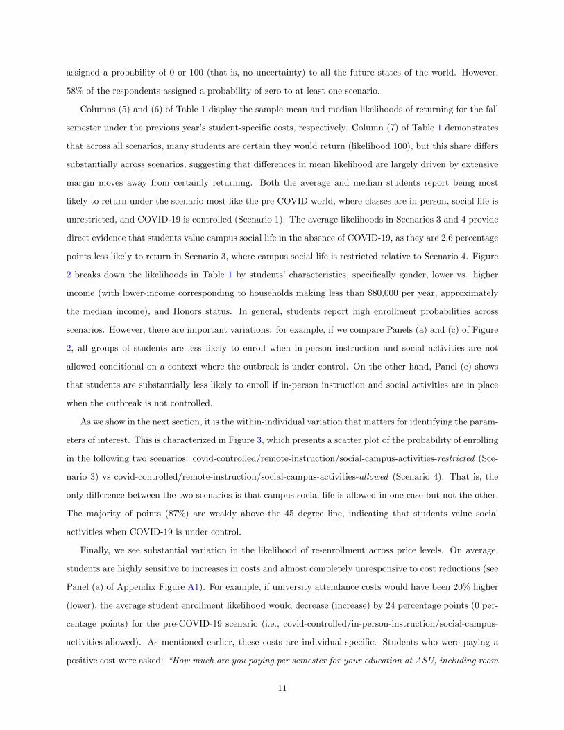

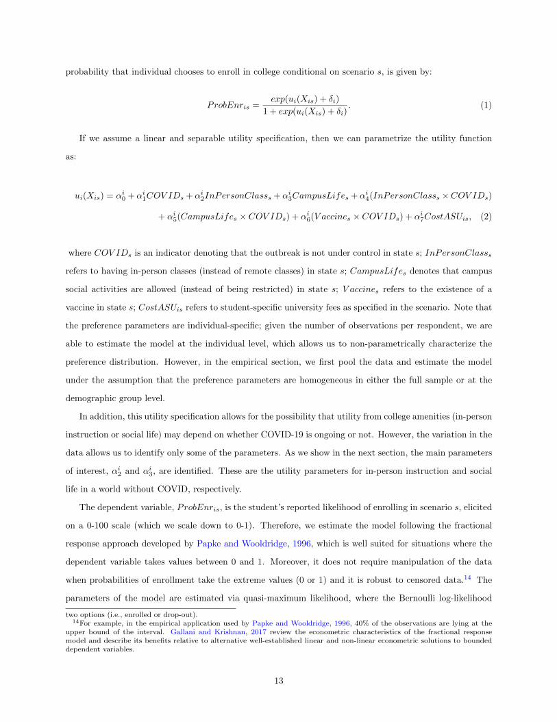
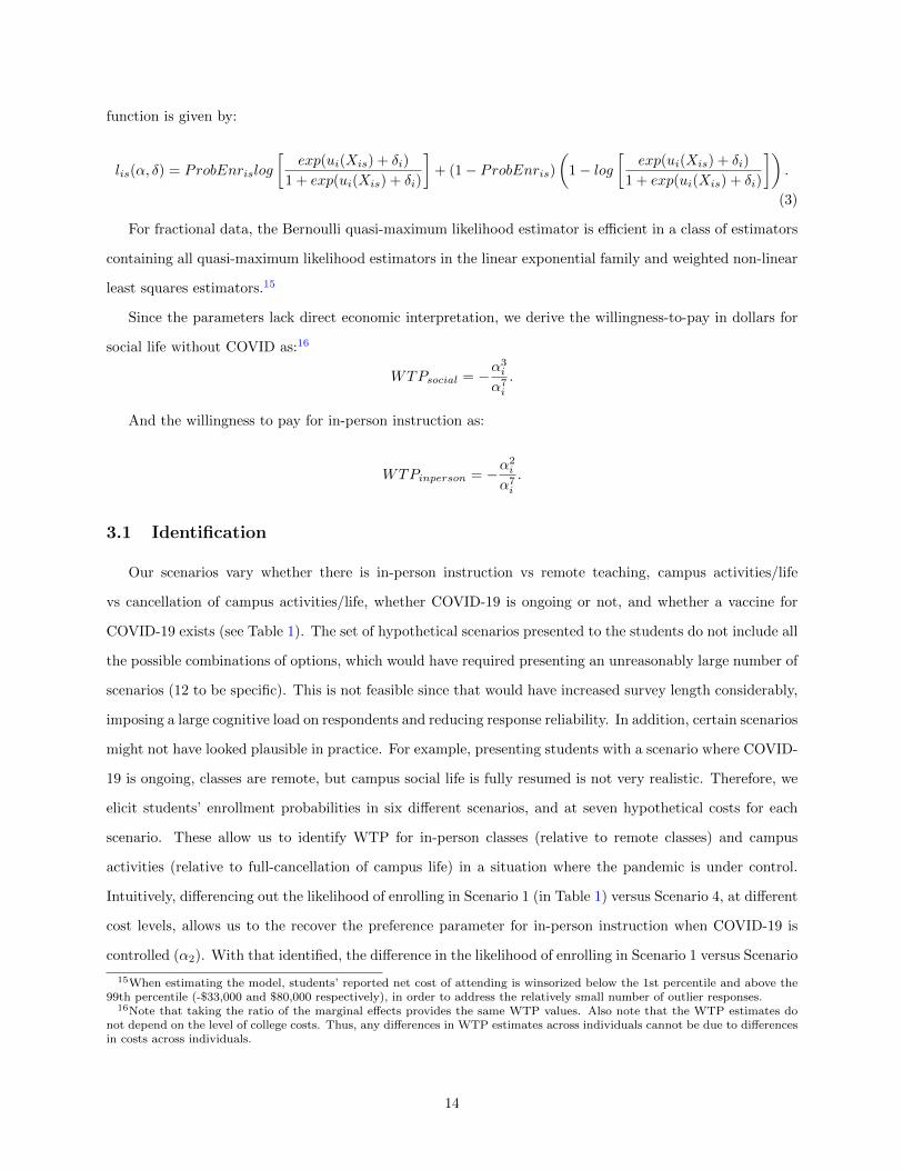


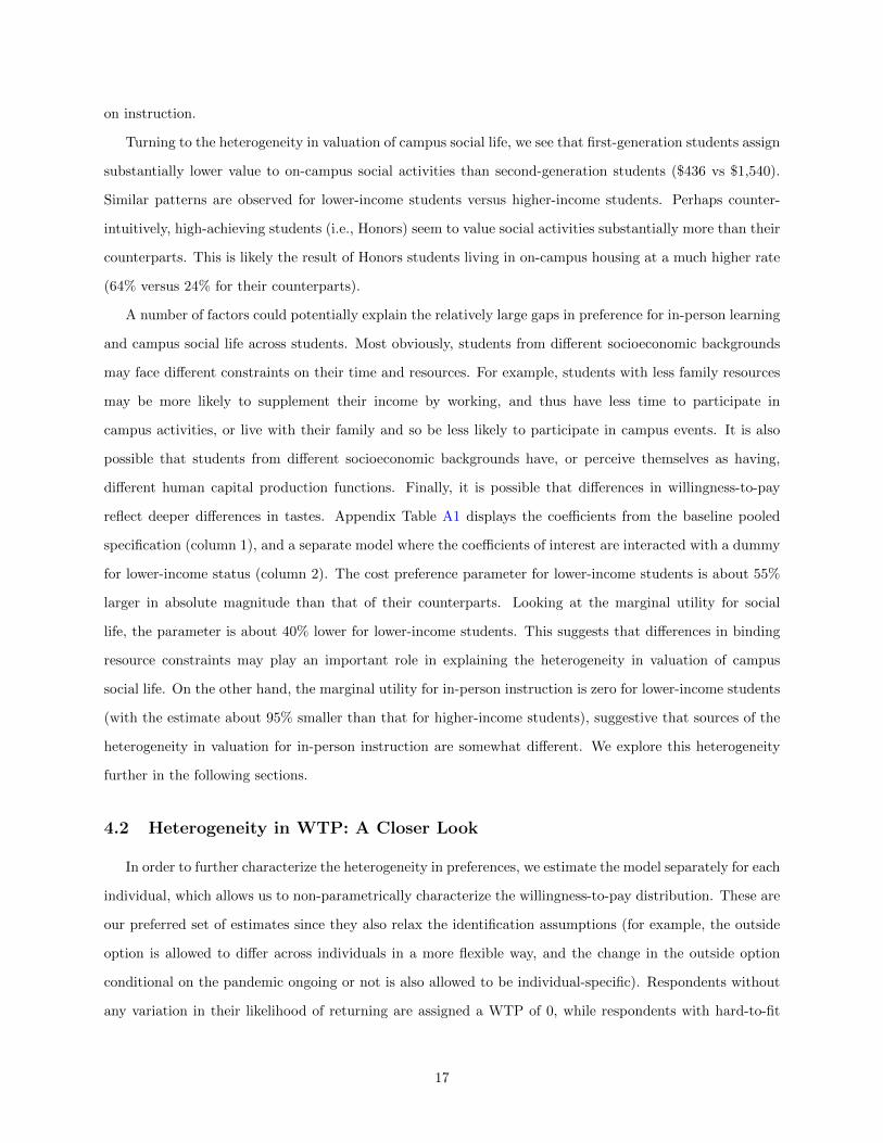
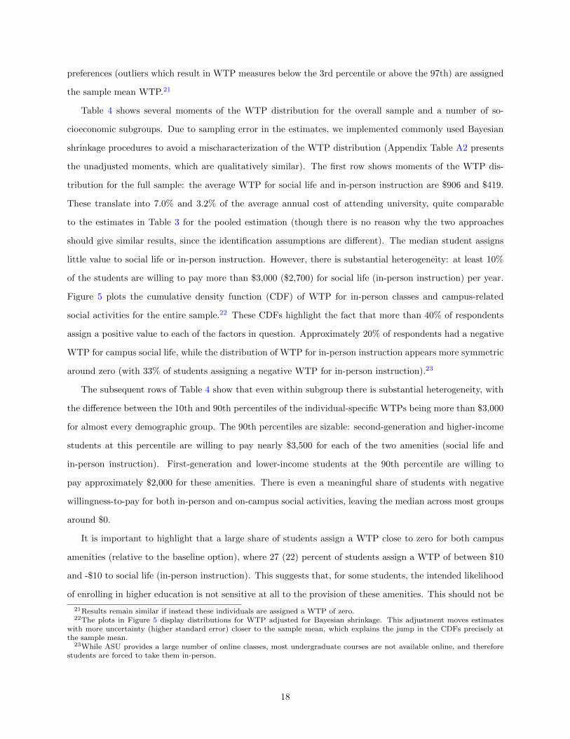
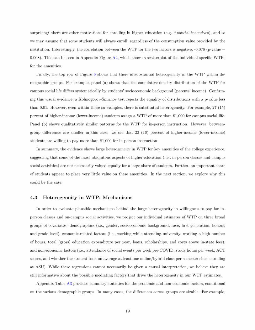

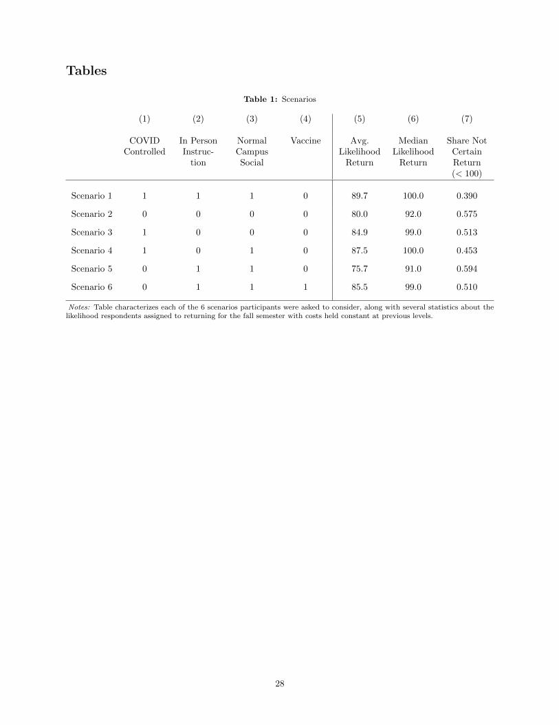
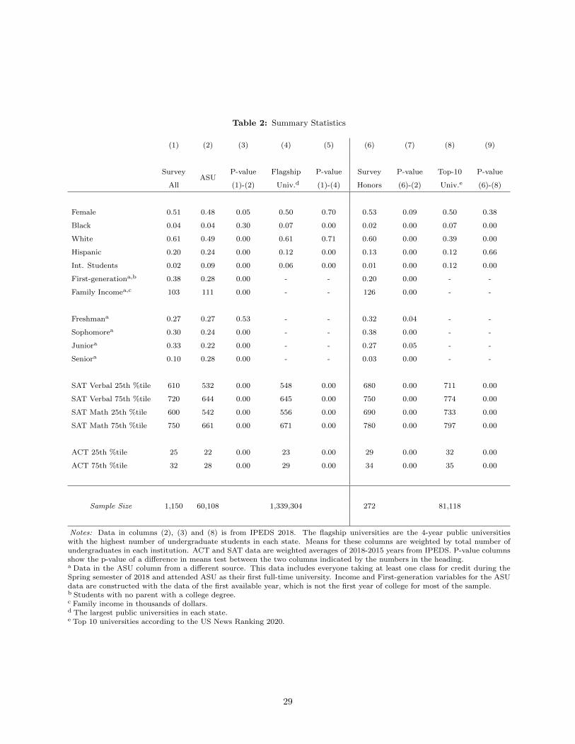

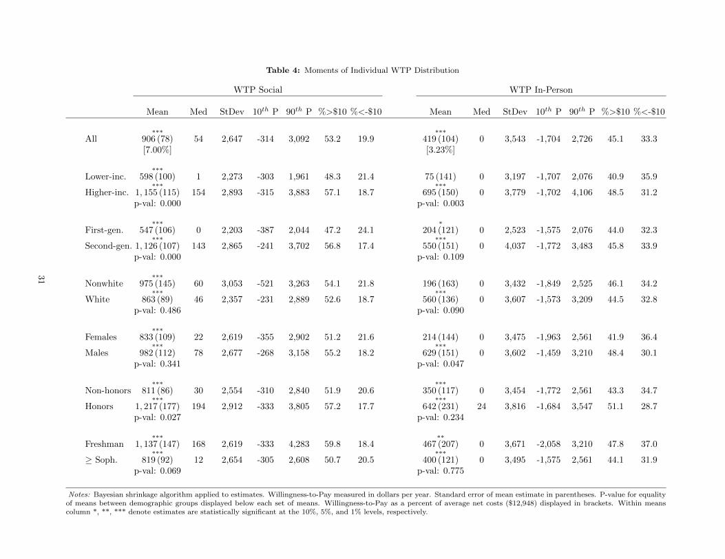


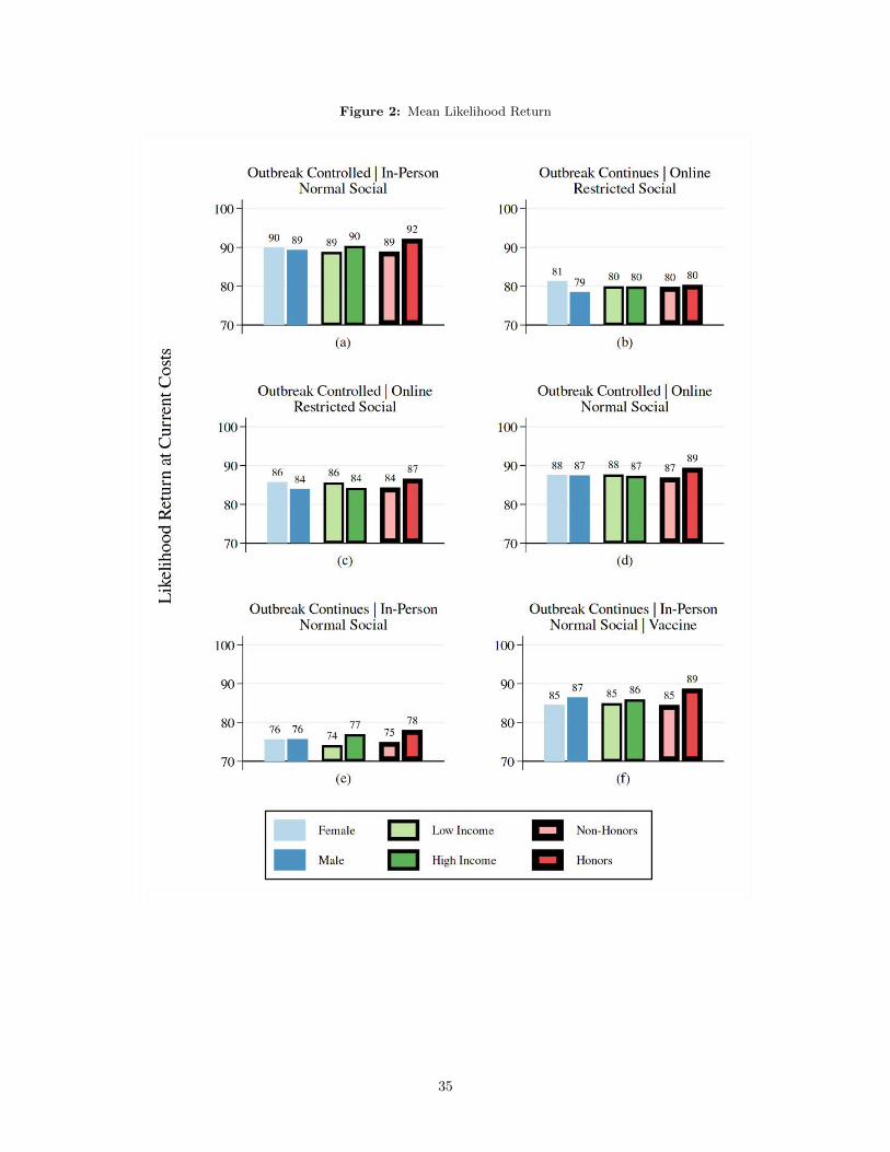

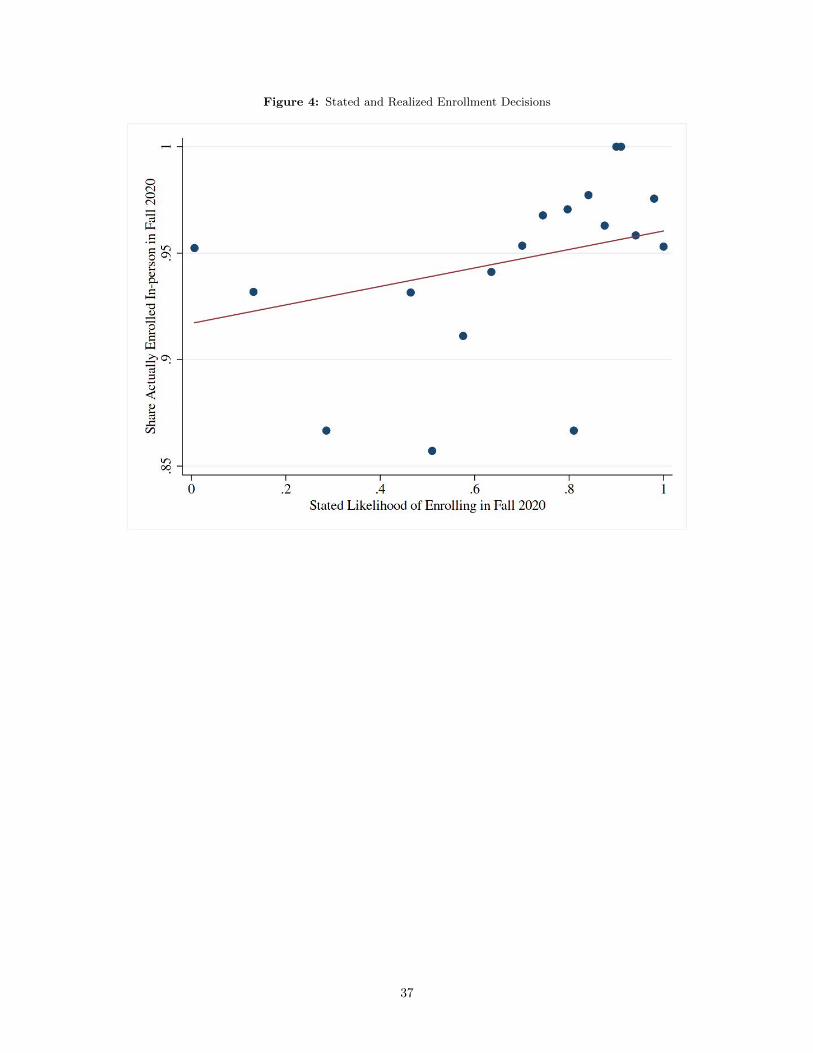

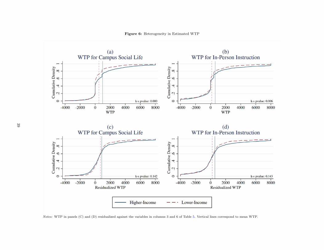


![enough to Estimating and Valuation...By: nissan URL: to Estimating and Valuation 3enough [1] INTRODUCTION An estimate is a computation or calculation of the quantities required and](https://static.documents.pub/doc/80x56/5e9bb9c3b63b25155522dcdf/enough-to-estimating-and-valuation-by-nissan-url-to-estimating-and-valuation.jpg)