1
Estimating the “Effective Period” of Bilinear Systems with
Linearization Methods, Wavelet and Time-Domain Analysis:
From Inelastic Displacements to Modal Identification
Nicos Makris1 and Georgios Kampas2
1Professor, Dept. of Civil Engineering, University of Patras, Greece, GR 26500, [email protected] 2Civil Engineer, Robertou Galli 27, Athens, Greece, GR 11742, [email protected]
ABSTRACT
This paper revisits and compares estimations of the effective period of bilinear
systems as they result from various published equivalent linearization methods and
signal processing techniques ranging from wavelet analysis to time domain
identification. This work has been mainly motivated from modal identification studies
which attempt to extract vibration periods and damping coefficients of structures that
may undergo inelastic deformations. Accordingly, this study concentrates on the
response of bilinear systems that exhibit low to moderate ductility values (bilinear
isolation systems are excluded) and concludes that depending on the estimation
method used, the values of the “effective period” are widely scattered and they lie
anywhere between the period-values that correspond to the first and the second slope
of the bilinear system. More specifically, the paper shows that the “effective period”
estimated from the need to match the spectral displacement of the equivalent linear
system with the peak deformation of the nonlinear system may depart appreciably
from the time needed for the nonlinear system to complete one cycle of vibration.
Given this wide scattering the paper shows that for this low to moderate ductility
values (say 10 ) the concept of the “effective period” has limited technical value
and shall be used with caution and only within the limitations of the specific
application.
Keywords: Modal Period, Equivalent Linear Analysis, System Identification, Time-
Frequency Analysis, Yielding Structures, Statistical Linearization.
1. INTRODUCTION
The development of an equivalent linear system that approximates the maximum
displacement of a bilinear hysteretic system when subjected to dynamic loading goes
back to the seminal work of Caughey [1],[2]. By that time the elastic response
spectrum was well developed and understood, and had become a central concept in
earthquake engineering (Chopra [3] and references reported therein). Once available,
the main attraction of the elastic response spectrum is that it offers the most
significant features of the structural response without requiring knowledge of the time
history of the excitation; while, its limitation is that it is defined only in relationship to
elastic structures. Starting in the late 1950s researchers began recognizing the
importance of studying the response of structures deforming into their inelastic range
and this led to the development of the inelastic response spectrum (Veletsos and
Newmark [4], Veletsos et al. [5], Veletsos and Vann [6]).
In parallel with the development of inelastic response spectra in earthquake
engineering, there has been significant effort in developing equivalent linearization
techniques (Caughey [1],[2], Rosenblueth and Herrera [7], Roberts and Spanos [8],
Crandall [9], among others) in order to define equivalent linear parameters (natural
periods and damping ratios) of equivalent linear systems that exhibit comparable
2
response values to those of the nonlinear systems. While the initial efforts in
developing equivalent linearization techniques originated in the fields of random
vibration and structural mechanics, these techniques found gradually major
applications in earthquake engineering.
One of the major challenges in earthquake engineering is the estimation of the peak
inelastic deformation of yielding structures. Traditionally, seismic design has not been
carried out with nonlinear time-history analysis; instead, seismic deformation
demands are established with the maximum response of “equivalent” linear single-
degree-of-freedom (SDOF) systems via the use of linear elastic response spectra.
Thus, through the years various displacement base methods (Miranda and Ruiz-
Garcia [10] and references reported therein) have been proposed to estimate the
maximum inelastic displacements from the maximum displacement of equivalent
linear elastic SDOF systems. Accordingly, in earthquake engineering the main goal
when developing an equivalent linear system is that the peak elastic deformation, is
comparable to the peak deformation of the inelastic system. Nevertheless, this
exercise does not assure that these two “equivalent” systems will also have
comparable vibration characteristics –that they will need the same time to complete a
one vibration cycle.
Early studies on estimating the effective period of bilinear systems by comparing peak
spectral values when subjected to earthquake loading were published by Iwan and
Gates [11] and Iwan [12] after minimizing the root mean square (RMS) of the
difference between the spectral displacements of a bilinear system and a family of
potentially equivalent linear systems. Some 35 years later, Guyader and Iwan [13]
revisited this problem and offered refined expressions for a conservative estimation of
the effective period and damping of a class of yielding systems. Recently Giaralis and
Spanos [14] returned to the framework of stochastic equivalent linearization technique
and presented a methodology to derive a power spectrum which, while represents a
Gaussian stationary process it is compatible in a stochastic sense with a given design
spectrum. This power spectrum is then treated as the excitation spectrum to determine
the effective period and damping coefficient of the corresponding equivalent linear
system.
In the abovementioned “spectral” studies, the effective period of the equivalent linear
system is determined by minimizing the difference (error) of either the response
spectra (Iwan and Gates [11], Iwan [12], Guyader and Iwan [13]), or the response
histories of the nonlinear and the equivalent linear systems (Giaralis and Spanos [14]).
While the estimation of inelastic deformations has a central role in the performance of
earthquake resistant structures, the identification of vibration characteristics of
yielding structure is also receiving increasing attention mainly due to the growing
need for monitoring the structural health of civil infrastructure. Accordingly, within
the context of system identification, the effective period of a yielding system may be
understood as the prevailing vibration period (time needed to complete one vibration
cycle) of the response history and can be extracted with signal processing methods
which examine the response signal alone. The performance of these methods is also
assessed in this study in an effort to conclude whether the “effective” period that is
estimated in order to estimate inelastic displacement is a representative vibration
period of the inelastic system.
By the mid 1980s wavelet transform analysis had emerged as a unique new time-
frequency decomposition tool for signal processing and data analysis (Grosman and
Morlet [15]). At present, there is a wide literature available regarding its mathematical
formulation and its applications (Mallat [16], Addison [17], Newland [18] and
3
references reported therein). Given that wavelets are simple wavelike functions
localized in time they emerge as a most useful tool for extracting the dominant period
of the response of bilinear systems.
In parallel with the wavelet transform analysis, various powerful time-domain
methods have been developed and applied successfully to extract the dominant period
of signals. One of the most well known and powerful methods for linear systems in
the system identification community is the Prediction Error Method (PEM). It initially
emerged from the maximum likelihood framework of Aström and Bohlin [19] and
subsequently was widely accepted via the corresponding MATLAB [20]
identification toolbox developed following the theory advanced by Ljung [21], [22],
[23].
In this work the prediction error method is also employed to extract the dominant
effective period of the response of bilinear hysteretic systems and the results obtained
from this time domain method are compared with the results obtained with the above-
mentioned time-frequency analysis (wavelet transform) and the equivalent
linearization methods also introduced in this section.
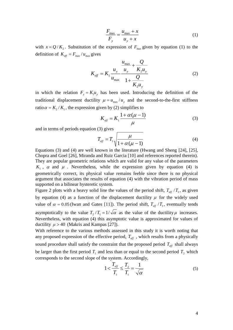
2. SIMPLE GEOMETRIC RELATIONS
The most elementary concept of an effective period of a system with bilinear behavior
is the period associated with effK , that is the slope of the line that connects that axis
origin with the point on the backbone curve where we anticipate the maximum
displacement, maxu , to occur. This concept of a secant stiffness was apparently first
proposed by Rosenblueth and Herrera [7] and then received wide acceptance for the
estimation of maximum inelastic displacement of yielding structures [Miranda and
Ruiz Garcia [10] and references reported therein).
With reference to Figure 1 one can derive via the use of similar triangles a relation
between the effective stiffness, effK and the first slope of the bilinear model, 1K .
According to Figure 1,
Figure 1. The hysteretic loop of the bilinear model.
4
max max
y y
F u x
F u x
(1)
with 2/x Q K . Substitution of the expression of maxF given by equation (1) to the
definition of max max/effK F u gives
max
2
1
max
2
1
y y y
eff
y
u Q
u u K uK K
Qu
K u
(2)
in which the relation 1y yF K u has been used. Introducing the definition of the
traditional displacement ductility max / yu u and the second-to-the-first stiffness
ratio 2 1/K K , the expression given by (2) simplifies to
)1(11
KK
eff (3)
and in terms of periods equation (3) gives
)1(11
TT
eff (4)
Equations (3) and (4) are well known in the literature (Hwang and Sheng [24], [25],
Chopra and Goel [26], Miranda and Ruiz Garcia [10] and references reported therein).
They are popular geometric relations which are valid for any value of the parameters
1K , and . Nevertheless, while the expression given by equation (4) is
geometrically correct, its physical value remains feeble since there is no physical
argument that associates the results of equation (4) with the vibration period of mass
supported on a bilinear hysteretic system.
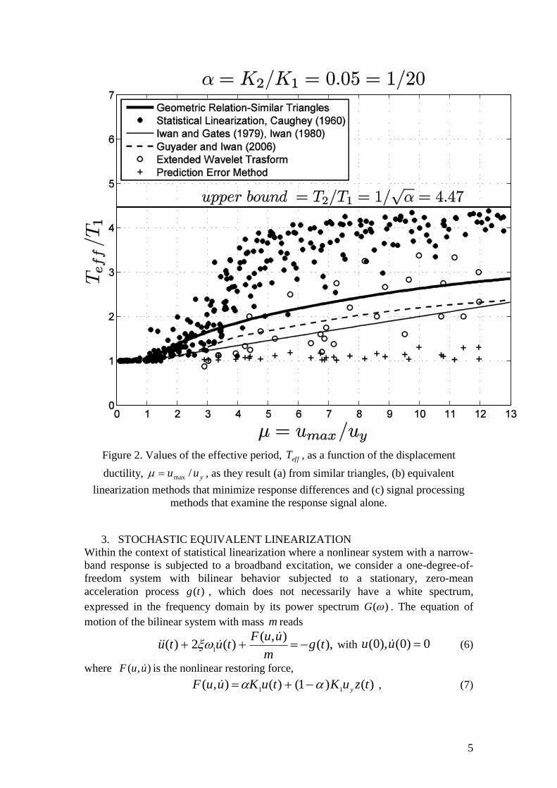
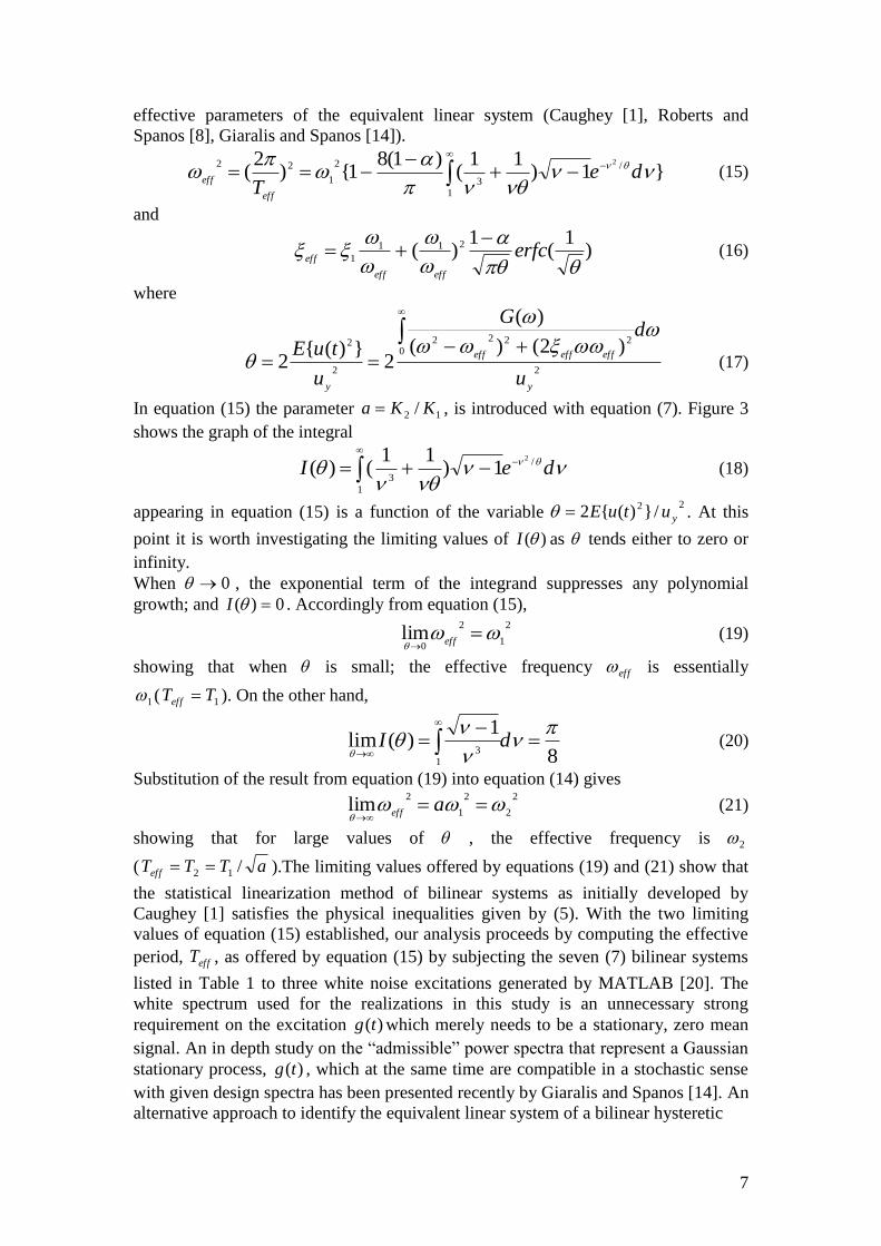
Figure 2 plots with a heavy solid line the values of the period shift, 1/TTeff , as given
by equation (4) as a function of the displacement ductility for the widely used
value of 05.0 (Iwan and Gates [11]). The period shift, 1/TTeff , eventually tends
asymptotically to the value /1/ 12 TT as the value of the ductility increases.
Nevertheless, with equation (4) this asymptotic value is approximated for values of
ductility 40μ (Makris and Kampas [27]).
With reference to the various methods assessed in this study it is worth noting that
any proposed expression of the effective period, effT , which results from a physically
sound procedure shall satisfy the constraint that the proposed period effT shall always
be larger than the first period 1T and less than or equal to the second period 2T which
corresponds to the second slope of the system. Accordingly,
11
1
2
1
T
T
T
Teff
(5)
5
Figure 2. Values of the effective period, effT , as a function of the displacement
ductility, yuu /max , as they result (a) from similar triangles, (b) equivalent
linearization methods that minimize response differences and (c) signal processing
methods that examine the response signal alone.
3. STOCHASTIC EQUIVALENT LINEARIZATION
Within the context of statistical linearization where a nonlinear system with a narrow-
band response is subjected to a broadband excitation, we consider a one-degree-of-
freedom system with bilinear behavior subjected to a stationary, zero-mean
acceleration process )(tg , which does not necessarily have a white spectrum,
expressed in the frequency domain by its power spectrum )(G . The equation of
motion of the bilinear system with mass m reads
),(),(
)(2)(1
tgm
uuFtutu
with 0)0(),0( uu (6)
where ),( uuF is the nonlinear restoring force,
)()1()(),(11
tzuKtuKuuFy
, (7)
6
in which 1K is the first slope of the bilinear loop, yu is the yield displacement shown
in Figure 1, 12 / KK is the ratio of the postyield stiffness 2K to the initial elastic
stiffness 1K , and )(tz is the internal dimensionless parameter with 1)( tz that is
governed by
0)()()()()()()(1
tutztutztztutzunn
y . (8)
The model given by equations (7) to (8) is the Bouc-Wen model (Wen [28], [29]) in
which , and n are dimensionless quantities that control the shape of the hysteretic
loop. Defining mK /1
2
1 equation (6) reduces to
)()]()1()([)(2)(2
11tgtzutututu
y (9)
The quantity )()1()(),( tzutuuu y appearing in equation (9) is a nonlinear
function that governs the restoring force-deformation law.
The nonlinear response )(tu appearing in equation (9) is approximated with the
response )(ty of an equivalent linear system with natural frequency eq and viscous
damping ratio eq given by the equation
),()()(2)(2
tgtytytyeffeffeff
with 0)0(),0( yy (10)
According to the original and most widely used form of statistical linearization
(Caughey [2], Roberts and Spanos [8], Giaralis and Spanos [14]) the parameters of the
linear system given by equation (9) are defined by minimizing the expected value of
the difference (error) between equations (9) and (10) in a least square sense with
respect to the quantities eff and eff . This criterion yields the following expressions
for the effective (equivalent) linear parameters
}{
)},()({)
2(
2
22
uE
uutuE
Teq
eff
(11)
and
}{
)},()({2
1
1uE
uutuE
eq
eff
(12)
where {.}E denotes the expectation operator. In most cases (Caughey [2], Roberts
and Spanos [8]) the unknown distribution of the response )(tu of the nonlinear
oscillator (bilinear system) is approximated for the purpose of evaluating the expected
values by a zero-mean Gaussian process. Furthermore, it is also assumed that the
variances of the process )(tu and )(ty are equal (Roberts and Spanos [8], Crandall
[9]). This leads to
d
GtuE
eqeqeq
02222
2
)2()(
)(})({ (13)
and
d
GtuE
eqeqeq
02222
2
2
)2()(
)(})({ (14)
where )(G is the power spectrum of the stationary, zero-mean acceleration process
)(tg . Substitution of equations (13) and (14) into the equations (11) an (12) gives the
7
effective parameters of the equivalent linear system (Caughey [1], Roberts and
Spanos [8], Giaralis and Spanos [14]).
}1)11
()1(8
1{)2
( /
13
2
1
22 2
de
Teff
eff
(15)
and
)1
(1
)( 211
1
erfc
effeff
eff
(16)
where
2
02222
2
2 )2()(
)(
2})({
2y
effeffeff
yu
dG
u
tuE
(17)
In equation (15) the parameter 12 / KKa , is introduced with equation (7). Figure 3
shows the graph of the integral
deI /
31
2
1)11
()(
(18)
appearing in equation (15) is a function of the variable 22 /})({2 yutuE . At this
point it is worth investigating the limiting values of )(I as tends either to zero or
infinity.
When 0 , the exponential term of the integrand suppresses any polynomial
growth; and 0)( I . Accordingly from equation (15), 2
1
2
0lim
eff
(19)
showing that when is small; the effective frequency eff is essentially
1 ( 1TTeff ). On the other hand,
8
1)(lim
13
dI
(20)
Substitution of the result from equation (19) into equation (14) gives 2
2
2
1
2lim
aeff
(21)
showing that for large values of , the effective frequency is 2
( aTTTeff /12 ).The limiting values offered by equations (19) and (21) show that
the statistical linearization method of bilinear systems as initially developed by
Caughey [1] satisfies the physical inequalities given by (5). With the two limiting
values of equation (15) established, our analysis proceeds by computing the effective
period, effT , as offered by equation (15) by subjecting the seven (7) bilinear systems
listed in Table 1 to three white noise excitations generated by MATLAB [20]. The
white spectrum used for the realizations in this study is an unnecessary strong
requirement on the excitation )(tg which merely needs to be a stationary, zero mean
signal. An in depth study on the “admissible” power spectra that represent a Gaussian
stationary process, )(tg , which at the same time are compatible in a stochastic sense
with given design spectra has been presented recently by Giaralis and Spanos [14]. An
alternative approach to identify the equivalent linear system of a bilinear hysteretic
8
Figure 3. Graph of the integral )(I appearing in equation (15).
system has been presented by Politopoulos and Feau [30] and references reported
therein.
Herein, we merely use white spectra in an effort to uncover the challenges associated
with the exercise to compute/identify the “effective period” of a bilinear system. Each
of the three MATLAB realizations was used to excite all 7 bilinear systems listed in
Table 1 and the levels of ductilities achieved were recorded. Subsequently, each
excitation was gradually amplified so that each bilinear system achieved various
levels of ductilitites up to the value of 12 . The bilinear systems listed in Table 1
have, 05.0a , and were selected so that their parameters ( yuT ,1 and Q ) correspond
to typical values of reinforced concrete and steel structures (see Table 1).
The response of the bilinear system is computed by solving equation (9) together with
equation (8). From the nonlinear response analysis the peak deformation maxu ,was
retained to compute the ductility demand of the response yuu /max .
The values of effT of all seven bilinear systems listed in Table 1 as they result from
statistical linearization via equation (15) are shown in Figure 2 with heavy dark dots
for various values of ductility levels. The majority of these dots lie well above the
Table I. Parameters of bilinear systems examined in this study with 05.0a
Model )(1 sT )(2 sT )(mu y )(/ gmQ
1 0.3 1.34 0.0050 0.212 2 0.4 1.79 0.0100 0.239 3 0.45 2.00 0.0026 0.05 4 0.5 2.24 0.0100 0.153 5 0.6 2.68 0.0200 0.212 6 0.67 3.00 0.0059 0.05 7 0.89 4.00 0.0104 0.05
9
heavy dark line –that is the geometric relation given by equation (4) and they tend to
accumulate close to the upper bound value aTT /12 . The differences between the
predictions of the effective period, effT , between equations (4) and (15) is anywhere
between 50% and 100%.
4. THE WORK OF IWAN AND GATES [11], IWAN [12] AND GUYADER
AND IWAN [13]
Early theoretical work of the effective period and damping of stiffness-degrading
structures was presented by Iwan and Gates [11]. The hysteretic model examined by
Iwan and Gates [11] is a collection of linear elastic and Coulomb slip elements which
can approximate the phenomenon of cracking, yielding and crushing. A special case
of their hysteretic model is the bilinear model that is of interest in this study. Their
study was motivated by the yielding response of traditional concrete and steel
structures where the initial elastic stiffness, 1K , is a dominant parameter of the model;
while, the displacement ductility assumes single digit values (say 8 ). Iwan and
Gates [11] observed that the average inelastic response spectra resemble the linear
response spectra except for a translation along an axis of constant spectral
displacement. The above observation was a major contribution at that time for it
indicates that the effective period of each corresponding linear system would be of
some constant multiple of the first period of the hysteretic system.
1effT CT (22)
Equation (22) is similar to equation (4); however, in the work of Iwan and Gates [11]
the constant, C , appearing in equation (22) is not an outcome from similar triangles
(which result by assuming that effK is the slope of the line that connects the axis origin
with the point on the backbone curve where we anticipate the maximum displacement
to occur), but is the outcome from minimizing the root mean square (RMS) of the
error between the average earthquake spectral displacements of a bilinear system and
a family of potentially equivalent linear systems. Table 2 compares the values of
C appearing in equation (22) for the bilinear system with 2 1/ 0.05K K as
computed by Iwan and Gates [11] together with the corresponding values of the term
))1(1/( appearing in equation (4).
Table II indicates that for moderate values of ductility, the period shift ( 1/effT T ) as
predicted by equation (4) is appreciably longer (i.e. 42% longer for 4.0 ) than the
Table II. Comparison of the Geometric Relation between effT and 1T and the Results
presented by Iwan and Gates [11] and Iwan [12].
max
y
u
u )1(1/(
0.05
1/effC T T
Iwan and
Gates [11]
Eq.(17)
Iwan
[12]
0.6 - 1.000 -
1.0 1.000 1.000 1.000
1.5 1.210 1.000 1.063
2.0 1.380 1.130 1.121
4.0 1.865 1.317 1.339
8.0 2.434 1.573 1.752
10
period shift computed by Iwan and Gates [11] after minimizing the RMS of the
difference between the equivalent elastic and inelastic average earthquake spectra.
Consequently, for moderate values of ductility ( 2.0 8.0 ) the findings of Iwan
and Gates [11] depart appreciably to the lower side from the results of the geometric
relation given by equation (4).
In a subsequent publication (Iwan [12]), the period shift, 1/effT T , presented in Table
II was graphed as a function of the ductility, max / yμ u u . The least square log-log fit
of these data resulted for a bilinear system with, 2 1/ 0.05K K , the following
expression
8,])1(121.01[1
939.0 TTeff
(23)
Figure 2 plots with a thin solid line the values of the period shift, 1
/TTeff
, as offered
by equation (23) for 0.05 and up to values of ductility, 12 . These values are
compared with the results from the geometric relation given by equation (4) and the
results from the statistical linearization formulation (dark dots) as they offered by
equation (15). What is striking about this comparison is that the differences between
equation (23) presented by Iwan [12] and equation (15) presented by Caughey [1] are
anywhere between 100% and 150%. Given that both methodologies are sound and
that their mathematical foundations are correct, the comparison of the values for the
effective period of bilinear systems offered in Figure 2 indicates that effT is a quantity
that has an elusive physical meaning, it depends strongly on the methodology adopted
to calculate it and shall be used with caution and only within the limitations of the
specific application.
At this point it is worth reiterating that the statistical linearization method as
formulated by Caughey [1] and documented by Roberts and Spanos [8]: (a) uses as
ground excitation a stationary, zero-mean acceleration process; and (b) the value of
effT result after minimizing the expected value of the difference (error) between the
displacement response time histories of the linear and nonlinear systems. On the other
hand, the method presented by Iwan and Gates [11] which leads to equation (23)
(Iwan [12]): (a) uses as ground excitation historic earthquake records; and (b) the
values of effT result after minimizing the overall RMS error between the average
spectral displacements of a bilinear system and a family of potentially equivalent
linear systems.
In view of these striking differences between the values of the estimated effT our
study proceeds with the estimation of the effective period, effT , by trying to identify a
dominant vibration period in the response of the bilinear system by using
mathematical formal and objective techniques.
Some 35 years later Guyader and Iwan [13] revisited the problem of estimating
equivalent linear parameters of nonlinear systems after introducing a measure on
“engineering acceptability” –that is conservative displacement predictions are more
acceptable than unconservative predictions. Building on the earlier work of Iwan and
Gates [11] and Iwan [12], Guyader and Iwan [13] presented the following set of
expressions for the period shift in a bilinear system
1
32 ])1(0178.0)1(1145.01[ TTeff , for 0.4 (24a)
1)]1(1240.01777.01[ TTeff , for 5.60.4 (24b)
11
1)]1)2(05.01
1(768.01[ TTeff
, for 5.6 (24c)
Figure 2 plots with a dashed line the values of the period shift 1/TTeff offered by
equations (24 a,b,c) for 05.0a up to values of ductility 12 . These values are
above the initial values proposed by Iwan and Gates [11], Iwan [12] given by
equations (23); yet, they remain below the over conservative values offered by the
geometric relation given by equation (4).
5. THE WORK OF GIARALIS AND SPANOS [14]
An effort to bridge the gap between the power spectrum appearing in stochastic
equivalent linearization (see equations (15) to (17)) and a design (earthquake)
acceleration spectrum, ),( effaS , was recently presented by Giaralis and Spanos
[14]. In their study, the core equation for relating aS to a one-sided power spectrum,
)(G representing a Gaussian stationary process )(tg assumes the expression
0222
2
,
22
,)2()(
)([})({),(
d
GtuES
effeff
effGeffeffGeffeffa(25)
in which the correction factor Geff , (coined as the “peak” factor in the original paper,
Giaralis and Spanos [14]) establishes the equivalence, with probability of exceedence
p , between the earthquake acceleration spectrum, aS and )(G (Vannmarcke [25]).
The exact determination of Geff , is associated with the first passage problem for
which a closed from solution is not available. In order to address this challenge,
Giaralis and Spanos [14] adopted a semi-empirical formula known to be reasonably
reliable for earthquake engineering applications (Vanmarcke [31], Der Kiureghian
[32]); while assuming that the aforementioned probability of exceedence is 5.0p .
The elaborated methodology presented by Giaralis and Spanos [14] eventually
involves a recursive procedure to evaluate )(G and its implementation is beyond the
scope of this study.
6. WAVELET ANALYSIS
In the above-reviewed equivalent linearization techniques (Caughey [1], Iwan and
Gates [11], Guyader and Iwan [13] and Giaralis and Spanos [14]) the effective period
of the bilinear system is estimated by engaging a linear system. The wavelet analysis,
presented in this section, examines the response signal alone without minimizing any
difference with the response of an equivalent linear oscillator.
Over the last two decades, wavelet transform analysis has emerged as a unique new
time-frequency decomposition tool for signal processing and data analysis. There is a
wide literature available regarding its mathematical foundation and its applications
(Mallat [16], Addison [17], Newland [18] and references reported therein). Wavelets
are simple wavelike functions localized on the time axis. For instance, the second
derivative of the Gaussian distribution, 2 / 2te
, known in seismology literature as the
symmetric Ricker wavelet (Ricker [33], [34] and widely referred as the “Mexican
Hat” wavelet, Addison [17]), 22 / 2( ) (1 ) tt t e (26)
is a widely used wavelet. Similarly the time derivative of equation (25) or a one cycle
cosine function are also wavelets. A comparison on the performance of various
12
symmetric and antisymmetric wavelet to fit acceleration records is offered in
Vassiliou and Makris [35]. In order for a wavelike function to be classified as a
wavelet, the wavelike function must have: (a) finite energy,
2( )E t dt
(27)
and (b) a zero mean. In this work we are merely interested to achieve a local matching
of the response history of a bilinear system with a wavelet that will offer the best
estimates of period, IT . Accordingly, we perform a series of inner products
(convolutions) of the acceleration response history of the bilinear system, ( )u t with
the wavelet ( )t by manipulating the wavelet through a process of translation (i.e.
movement along the time axis) and a process of dilation-contraction (i.e. spreading
out or squeezing of the wavelet)
( , ) ( ) ( ) ( )t
C s w s u t dts
(28)
The values of s S and , for which the coefficient, , ,C s C S becomes
maximum offer the scale and location of the wavelet t
w ss
that locally best
matches the acceleration record, tu . Equation (28) is the definition of the wavelet
transform. The quantity ( )sw outside the integral in equation (28) is a weighting
function. Typically ( )sw is set equal to s1/ in order to ensure that all wavelets
,s
tt w s
s
at every scale s have the same energy, and according to
equation (27)
2
2
, , 2
1,s s
tt dt dt t constant s
ss
(29)
The same energy requirement among all the daughter wavelets ,s t is the default
setting in the MATLAB wavelet toolbox and has been used by Baker [36]; however,
the same energy requirement is, by all means, not a restriction. Clearly there are
applications where it is more appropriate that all daughter wavelets ,s t at every
scale s to enclose the same area ( ( ) 1/w s s ) or have the same maximum value
( ( ) 1w s ). However, in this paper there is no particular need for not using the default
same energy requirement for the daughter wavelets.
The multiplication factor
2
,,
C SS
w s S E
(30)
where E is the energy of the mother wavelet, is needed in order for the best matching
wavelet, ,S
tt w s
S
, to assume locally the amplitude of the
acceleration record.
13
One of the challenges with any given wavelet is that upon is selected as the
interrogating signal there is a commitment on the phase and the number of cycles of
the mother wavelet. This challenge has been recently addressed by Vassiliou and
Makris [35] who proposed the extended wavelet transform where in addition to a time
translation and a dilation-contraction, the proposed transform allows for a phase
modulation and the addition of half cycles.
In the classical wavelet transform defined with equation (28) the mother wavelet is
only subjected to a translation together with a dilation-contraction, t
s
. The
dilation contraction is controlled with the scale parameter s ; while, the movement of
the wavelet along the time axis is controlled with the translation time, . For instance,
any daughter wavelet of the symmetric Ricker mother wavelet given by equation (26)
assumes the form
212
21
t
st te
s s
(31)
In equation (31) the relation between the scale of the wavelet s and the period of the
pulse, pp fT /1 is 2/2pTs (Addison [17]). The need to include four
parameters in a mathematical expression of a simple wavelike function has been
presented and addressed by Mavroeidis and Papageorgiou [37]. They identified as the
most appropriate analytical expression the Gabor [38] “elementary signal” which they
slightly modified to facilitate derivations of closed-form expressions of the spectral
characteristics of the signal and response spectra. The Gabor [38] “elementary signal”
is defined as
2
22
cos 2
pft
pg t e f t
(32)
which is merely the product of a harmonic oscillation with a Gaussian envelop. In
equation (32), pf is the frequency of the harmonic oscillation, is the phase angle
and
is a parameter that controls the oscillations characters of the signal. The Gabor
wavelike signal given by equation (32) does not have a zero mean; therefore, it cannot
be a wavelet within the context of the wavelet transformation.
Nevertheless, the elementary signal proposed by Mavroeidis and Papageorgiou [37] to
approximate velocity pulses is a slight modification of the Gabor signal given by
equation (32) where the Gaussian envelope has been replaced by an elevated cosine
function.
21
1 cos cos 22
p
p
fv t t f t
(33)
Clearly the wavelike signal given by equation (33) does not always have a zero mean;
therefore it cannot be a wavelet within the context of wavelet transform. Nevertheless,
the time derivative of the elementary velocity signal given by equation (33)
2 2sin cos 2 sin 2 1 cos
p p p
p p
f f fdv tt f t f t t
dt
(34)
14
is by construction a zero-mean signal and is defined in this paper as the Mavroeidis
and Papageorgiou (M&P) wavelet. After replacing the oscillatory frequency, pf , with
the inverse of the scale parameter the M&P wavelet is defined as
2 2 2 2
, , sin cos sin 1 cost
t t t ts s s s s
(35)
The novel attraction in the M&P wavelet given by equation (35) is that in addition to
the dilation-contraction and translation t
s
, the wavelet can be further
manipulated by modulating the phase, , and the parameter , which controls the
oscillatory character (number of half cycles). We can now define the four parameter
wavelet transform as
( , , , ) ( , , ) ( ) ( , , )t
C s w s u t dts
(36)
The inner product given by equation (36) is performed repeatedly by scanning not
only all times, , and scales, s , but also by scanning various phases,
{0, / 4, / 2,3 / 4} , and various values of oscillatory character of the signal
{1.0,1.5,2.0,2.5,3.0} . When needed more values of and may be scanned. The
quantity ( , , )w s outside the integral is a weighting function which is adjusted
according to the application. For instance, when all daughter wavelets have the same
area the wavelet transform emphasizes on the shorter period pulses; whereas when all
daughter wavelets have the same amplitude the wavelet transform emphasizes on the
longer period pulses (Vassiliou and Makris [35]).
Figure 4 (top-left) plots with a heavy dark line the best matching Mavroeidis and
Papageorgiou (M&P) wavelet (Vassiliou and Makris [35]) on the acceleration
response history of a bilinear system with strength / 0.153Q m g , first period
1 0.5T s and 0.01 1yu m cm when subjected to the OTE ground motion recorded
during the 1995 Aigion earthquake. The displacement ductility reached is
max / 6.76yu u and the period of the best matching wavelet –that is the dominant
vibration period is 1.20effT s . Figure 5 (left) plots the 5% elastic displacement
response spectrum of the OTE ground motion -1995 Aigion earthquake and for the
period 1.20effT s as extracted with the wavelet analysis, the elastic spectral
displacement is 0.06DS m . Note that the dominant pulse extracted with wavelet
analysis depends on the weighting function, ( , , )w s appearing in front of the
integral given by equation (36) (Vassiliou and Makris [35]). In this analysis
( , , )w s is selected in such a way so that all daughter wavelets in the analysis have
the same energy. Next to this spectral value that corresponds to a displacement
ductility of the inelastic system , 6.76 , the period values (and the corresponding
spectral displacement) offered by equations (23) ( & 0.81I GT s ) and (24)
( sT IG 94.0& ) and the geometric relation given by equation (4) ( 1.15STT s ) are
shown. Note that in this example the vibration period extracted with the wavelet
analysis is longer than the period predicted with the minimization proposed by Iwan
15
and Gates [11] which is always shorter than the period which one computes with
similar triangles (equation (4)). The spectral displacement that correspond to the
vibration period extracted with the wavelet analysis ( 1.20WAT s ) is 0.06SD m ;
Figure 4. Matching the acceleration response histories of bilinear systems with
wavelet analysis (top) and the Prediction Error Method (center) when they are
subjected to records from the 1995 Aigion, Greece and the 1979 Coyote Lake
earthquakes.
16
Figure 5.Elastic displacement response spectra of the two earthquake records shown
in Figure 4(bottom) together with the effective period values of two bilinear systems
as they result from the methods assessed in this study.
while 0.08SD m and more than 0.10m when equations (18) and (4) are used
respectively.
Figure 4 (top-right) plots with a heavy dark line the best matching M&P wavelet
(Vassiliou and Makris [35]) on the acceleration response history of a bilinear system
with strength / 0.239Q m , first period 1 0.4T s and 0.01yu m when subjected to
Gilroy Array #6 ground motion recorded during the 1979 Coyote Lake earthquake.
The displacement ductility reached is max / 7.25yu u and the period of the best
matching wavelet –that is the dominant vibration period is 2.75effT s .
Figure 5 (right) plots the 5% elastic displacement response spectrum of the Gilroy
Array #6 ground motion -1995 Coyote Lake earthquake. For the period 2.75effT s as
extracted with the wavelet analysis the spectral displacement is 0.014SD m . Next to
this spectral value that corresponds to a displacement ductility of the inelastic system,
7.25 , the period values offered by equations (23) ( & 0.67I GT s ) and (24)
( sT IG 94.0& ) and the geometric relation given by equation (4) ( 0.94STT s ) are
shown.
Table III. Earthquake records selected as input motions in this study.
Earthquake Record Station Magnitude, w
M PGA(g)
1966 Parkfield CO2 (St. 065) 6.0 0.48
1979 Coyote Lake, CA Gilroy Array #6 230 5.7 0.43
1983 Coalinga Oil City 270 5.8 0.87
1983 Coalinga Transmitter Hill 360 5.8 1.08
1983 Coalinga Transmitter Hill 270 5.8 0.84
1986 North Palm Springs North Palm Springs 6.1 0.69
1995 Aigion OTE Building 6.2 0.54
The vibration periods extracted with wavelet analysis from the response of all bilinear
systems listed in Table II when subjected to the historic records listed in Table III are
also shown in Figure 2 with empty circles. These values are scattered, nevertheless,
17
most of them lie above the line defined by equation (18) (Iwan and Gates [11], Iwan
[12]).
7. TIME DOMAIN ANALYSIS
Over the years, various powerful time domain methods have been developed and
applied successfully. Perhaps, the most well known and powerful method in the
system identification community is the Prediction Error Method (PEM).
It initially emerged from the maximum likelihood framework of Aström and Bohlin
[19] and subsequently was widely accepted via the corresponding MATLAB [20]
identification toolbox developed following the theory advanced by Ljung [21], [22],
[23].
Figure 4(center-left) plots with a heavy dark line the signal generated with the
prediction error method (PEM) that best identifies the acceleration response history of
bilinear system with strength / 0.155Q m g , first period 1 0.5T s and
0.01 1yu m cm when subjected to the OTE ground motion recorded during the 1995
Aigion earthquake. The period if the best matching signal offered by PEM is
1.02effT s . While the wavelet analysis (see Figure 4 top-left) concentrates on
matching locally the most energetic pulse of the response history the prediction error
method attempts to match to the extent possible a maximum segment of the response
history. Consequently, the effective vibration period extracted with PEM will be in
principle shorter than the periods extracted with wavelet analysis. Figure 4 (center-
right) plots with a heavy dark line the signal generated with PEM that best identifies
the acceleration response history of a bilinear system with strength / 0.239Q m g ,
first period, 1 0.4T s and 0.01yu m when subjected to the Gilroy Array #6 ground
motion recorded during the 1979 Coyote Lake earthquake. In this case the period of
the best matching identification signal offered by PEM is 1.01effT s ; whereas the
period of the best matching wavelet (see Figure 4 center left) is 2.75effT s . The
shape of the Gilroy Array #6 spectrum shown in Figure 5(right) is such that these two
period values which are 2.75 1.01 1.74s apart correspond to comparable spectral
displacements.
The vibration periods extracted with the prediction error method from the response of
all bilinear systems listed in Table II are also shown in Figure 2 with crosses. These
values are systematically close to the value of the first period, 1T , of the bilinear
system, indicating that the PEM tends to extract essentially the elastic period that
manifest itself during the small-amplitude vibrations. The poor performance of the
PEM in identifying the equivalent linear modal properties of 2-DOF systems with
bilinear isolators has also been reported by Kampas and Makris [33].
8. CONCLUSIONS
This paper revisits and compares estimations of the effective period of bilinear
systems exhibiting low to moderate ductility values as they result from: (a) Simple
geometric relations associated with the bilinear loop, (b) stochastic equivalent
linearization where the excitation process has a white spectrum, (c) the equivalent
linearization method which minimize the difference between earthquake spectra
presented by Iwan and Gates [11] and Guyader and Iwan [13], (d) best matching the
most energetic pulse of the nonlinear response history with a four-parameter wavelet
and (e) a time-domain method known as the Prediction Error Method (PEM).
18
The general conclusion is that the resulting values of the “effective period” (vibration
period of the equivalent linear system) are widely scattered and they lie anywhere
between the period values that correspond the first and the second slope of the bilinear
system.
At any given ductility value, max / yu u , the simple geometric relation,
1 / [1 ( 1)]effT T a appears to give the average value of effT among the scattered
values offered by the aforementioned methods as summarized in Figure 2.
The stochastic equivalent linearization method in which the excitation process has a
white spectrum yields effective period values which are systematically larger than the
period values offered by the simple geometric relation, 1 / [1 ( 1)]effT T a ;
while, the equivalent linearization method which minimizes the difference between
the earthquake spectra (Iwan and Gates [11]) yields effective period values which are
appreciable shorter. The revised expressions of Guyader and Iwan [13] which
accounted for a conservative estimation of the effective period yield effective period
values longer than the initial estimates of Iwan and Gates [12]; yet, shorter than the
simple geometric relation.
In addition to methods (b) and (c), the study examined the performance of two signal
processing methods that process the response history alone without minimizing any
difference with the response of a potentially equivalent linear oscillator.
The best matching of the most energetic pulse of the nonlinear response history with a
four-parameter wavelet transform yields vibration (“effective”) period values which
are widely scattered confirming the main finding of this study that the concept of the
“effective period” of a bilinear system has limited technical value and the results
depend strongly on the methodology used.
Finally, the study show that the prediction error method attempts to match to the
extent possible, a maximum segment of the nonlinear response history; therefore,
concentrating on the small amplitude part of the nonlinear response; while, missing
the local longer-period pulses which develop when the bilinear system experiences its
larger ductility values.
ACKNOWLEDGEMENTS
This research has been co-financed by the European Union (European Social Fund –
ESF) and Greek national funds through the Operational Program "Education and
Lifelong Learning" of the National Strategic Reference Framework (NSRF) -
Research Funding Program: Heracleitus II. Investing in knowledge society through
the European Social Fund.
REFERENCES
1. Caughey, T.K. Random excitation of a system with bilinear hysteresis. Journal
of Applied Mechanics 1960; 27,649-652.
2. Caughey, T.K. Equivalent linearization techniques. Journal of Acoustical
Society of America 1963; 35,1706-1711.
3. Chopra A. Elastic response spectrum: A historical note. Journal of Earthquake
Engineering and Structural Dynamics 2007; 36, 3-12.
4. Veletsos A.S., and Newmark, N.M. Effect of inelastic behavior on the
response of simple systems to earthquake motions. In: Proceedings of the
second world conference on earthquake engineering, Japan 1960; 2,895-912.
19
5. Veletsos A.S., Newmark N.M., Chelepati C.V. Deformation spectra for elastic
and elastoplastic systems subjected to ground shock and earthquake motions.
Proceedings of the 3rd World Conference on Earthquake Engineering, vol. II,
Wellington, New Zealand 1969, 663-682.
6. Veletsos A.S., Vann W.P. Response of ground-excited elastoplastic systems.
Journal of Structural Division (ASCE) 1971; 97(ST4),1257-1281.
7. Rosenblueth E, Herrera I. On a kind of hysteretic damping. Journal of
Engineering Mechanics Division ASCE, 1964; 90:37– 48.
8. Roberts J.B and Spanos P.D. Random vibration and statistical Linearization.
New York: Dover Publications, 1990.
9. Crandall, S.H. A half-century of stochastic equivalent linearization. Journal of
Structural Control and Health Monitoring 2006; 13:27-40.
10. Miranda, E., and Ruiz-Garcia, J. Evaluation of approximate methods to
estimate maximum inelastic displacement demands. Journal of Earthquake
Engineering and Structural Dynamics, 2002; 31, 539-560.
11. Iwan W.D., and Gates N.C. The effective period and damping of a class of
hysteretic structures. Journal of Earthquake Engineering and Structural
Dynamics 1979; 7,199-211.
12. Iwan W.D. Estimating inelastic response spectra from response spectra.
Journal of Earthquake Engineering and Structural Dynamics 1980, 8,375-388.
13. Guyader, A., C., and Iwan, W., D. Determining Equivalent Linear Parameters
for Use in a Capacity Spectrum Method of Analysis. Journal of Structural
Engineering, 2006; 132, 59-67.
14. Giaralis A., and Spanos P.D. Effective linear damping and stiffness
coefficients of nonlinear systems for design spectrum base analysis, Journal of
Soil Dynamics and Earthquake Engineering 2010; 30, 798-810.
15. Grossman, A. and Morlet, J. Decomposition of Hardy functions into square
integrable wavelets of constant shape, SIAM J. Math. Anal. 1984; 15(4):723-
736.
16. Mallat S. G. A wavelet tour of signal processing. Academic Press, 1999.
17. Addison P. S. The illustrated wavelet transform handbook. Institute of Physics
Handbook, 2002.
18. Newland, D.E. An Introduction to Random Vibrations, Spectral and Wavelet
Analysis, Third Edition, Longman Singapore Publishers, 1993.
19. Aström, K. J., and Bohlin T. Numerical identification of linear dynamic
systems from normal operating records. IFAC Symposium on Self-Adaptive
Systems, Teddington, England, 1965.
20. MATLAB. High-performance Language Software for Technical Computation.
The MathWorks, Inc: Natick, MA, 2002.
21. Ljung L. System Identification-Theory for the User, Prentice-Hall, New
Jersey, 1987.
22. Ljung L. State of the Art in Linear System Identification: Time and Frequency
Domain Methods. Proceedings of ’04 American Control Conference 1994;
1,650-660.
23. Ljung L. Prediction Error Estimation Methods. Circuits Systems Signal
Processing 2002; 21: 11-21.
24. Hwang, J.S., and Sheng L.H. Equivalent elastic seismic analysis of base-
isolated bridges with lead-rubber bearings. Journal of Engineering Structures,
1993; 16(3),201-209.
20
25. Hwang, J.S., and Sheng L.H. Effective stiffness and Equivalent Damping of
Base-Isolated Bridges. Journal of Structural Engineering, 1994; 119(10),
3094-3101.
26. Chopra, A., and Goel, R., K. Evaluation of NSP to Estimate Seismic
Deformation: SDF Systems. Journal of Structural Engineering, 2000; 126(4),
482-490.
27. Makris N., and Kampas G. The Engineering Merit of the “Effective Period” of
Bilinear Isolation Systems, Earthquakes and Structures, in press.
28. Wen Y., K. Approximate method for nonlinear random vibration. Journal of
Engineering Mechanics 1975; 101(4), 389-401.
29. Wen Y., K. Method for random vibration of hysteretic systems. Journal of
Engineering Mechanics 1976; 102(2), 249-263.
30. Politopoulos, I., and Feau, C. Some aspects of floor spectra of 1DOF
nonlinear primary structures. Journal of Earthquake Engineering and
Structural Dynamics. 2007; 36:975–993.
31. Vanmarcke EH. Structural response to earthquakes. Seismic Risk and
Engineering Decisions. Amsterdam: Elsevier, 1976.
32. Der Kiureghian A. Structural response to stationary excitation. Journal of
Engineering Mechanics, ASCE, 1980; 106,1195-213.
33. Ricker, N. Further developments in the wavelet theory of seismogram
structure. Bull. Seism. Soc. Am 1943; 33, 197-228.
34. Ricker N. Wavelet functions and their polynomials. Geophysics 1944;9, 314–
323.
35. Vassiliou, M., F., and Makris, N. Estimating Time Scales and Length Scales
in Pulselike Earthquake Acceleration Records with Wavelet Analysis. Bull.
Seism. Soc. Am. 2011; 101(2), 596-618.
36. Baker, W.J., Quantitative classification of near fault ground motions using
wavelet analysis, Bull. Seism. Soc. Am., 2007; 97, 1486-1501.
37. Mavroeidis, G. P., A. S. Papageorgiou A mathematical representation of near-
fault ground motions, Bull. Seism. Soc. Am. 2003; 93, 1099-1131.
38. Gabor, D.,Theory of communication. I. The analysis of information, IEEE
1946;93, 429–441.