Estimating the Gains from Liberalizing Services Trade: The Case of Passenger Aviation * ∗ Anca D. Cristea, University of Oregon David Hummels, Purdue University & NBER Brian Roberson, Purdue University April 2017 Preliminary. Comments Welcome Abstract: Over a 22-year period the US signed 106 bilateral “Open Skies Agreements” that significantly liberalized international trade in passenger aviation services. We study how existing trade agreements distorted route structures, carrier entry and capacity, and how liberalization affected consumer welfare. We develop a novel two-stage game in which carriers first enter and decide on networks, then set capacity and a pricing schedule prior to the realization of uncertain demand. The model allows for three empirically relevant features of airline markets: carriers have unused capacity; prices vary across carriers due to quality; for otherwise identical seats, prices rise as planes near capacity and are sold only to highest valuation passengers. We further show that even complex network environments can be described in terms of average pricing functions that map closely into empirical objects. We evaluate the model using difference-in-difference regressions applied to a 16-year panel of detailed data on route structure, capacity, and ticket price, quantity, and quality. Liberalizing countries see expansions in route offerings and reallocations of carrier capacity, consistent with mechanisms highlighted in the model. Consumers enjoy lower prices, more direct flights, and large increases in passenger quantities conditional on prices and on direct measures of quality. These effects are not uniform across cities. Quality adjusted prices fall by 7 percent on routes that were the least constrained prior to regulation, and by 15.3 percent on the most constrained routes. JEL: F13; L43; L93 Keywords: Services; Trade liberalization; Air transport; Open Skies Agreements. * This paper has benefited from many helpful discussions. We particularly thank Jack Barron, Bruce Blonigen, Tim Cason, Joe Francois, Giovanni Maggi, Steve Martin, Anson Soderbery, Bob Staiger, and Dan Trefler, and seminar participants at Dartmouth, ITAM, Monash, Penn, Penn State, Purdue, Toronto, the World Bank, and Yale and at several conferences including: CEPR GIST, EIIT, ETSG, Midwest International, and the West Coast Trade Conference. We also thank John Lopresti for excellent research assistance. Any remaining errors are our own.
Transcript
Estimating the Gains from Liberalizing Services Trade:
The Case of Passenger Aviation*∗
Anca D. Cristea, University of Oregon
David Hummels, Purdue University & NBER
Brian Roberson, Purdue University
April 2017
Preliminary. Comments Welcome
Abstract:
Over a 22-year period the US signed 106 bilateral “Open Skies Agreements” that significantly liberalized international trade in passenger aviation services. We study how existing trade agreements distorted route structures, carrier entry and capacity, and how liberalization affected consumer welfare. We develop a novel two-stage game in which carriers first enter and decide on networks, then set capacity and a pricing schedule prior to the realization of uncertain demand. The model allows for three empirically relevant features of airline markets: carriers have unused capacity; prices vary across carriers due to quality; for otherwise identical seats, prices rise as planes near capacity and are sold only to highest valuation passengers. We further show that even complex network environments can be described in terms of average pricing functions that map closely into empirical objects. We evaluate the model using difference-in-difference regressions applied to a 16-year panel of detailed data on route structure, capacity, and ticket price, quantity, and quality. Liberalizing countries see expansions in route offerings and reallocations of carrier capacity, consistent with mechanisms highlighted in the model. Consumers enjoy lower prices, more direct flights, and large increases in passenger quantities conditional on prices and on direct measures of quality. These effects are not uniform across cities. Quality adjusted prices fall by 7 percent on routes that were the least constrained prior to regulation, and by 15.3 percent on the most constrained routes.
JEL: F13; L43; L93
Keywords: Services; Trade liberalization; Air transport; Open Skies Agreements.
* This paper has benefited from many helpful discussions. We particularly thank Jack Barron, Bruce Blonigen, Tim Cason, Joe Francois, Giovanni Maggi, Steve Martin, Anson Soderbery, Bob Staiger, and Dan Trefler, and seminar participants at Dartmouth, ITAM, Monash, Penn, Penn State, Purdue, Toronto, the World Bank, and Yale and at several conferences including: CEPR GIST, EIIT, ETSG, Midwest International, and the West Coast Trade Conference. We also thank John Lopresti for excellent research assistance. Any remaining errors are our own.
2
1. Introduction
Services represent a large (20 percent) and growing share of world trade, but the exact
reasons for that growth are not immediately clear. Growth in services trade may simply reflect
the rising share of services in employment and output worldwide, or be due to trade facilitating
improvements in information technology and telecommunications.1 It may also be that a
sustained focus on liberalizing services trade through the WTO / General Agreement on Trade in
Services (GATS) and through bilateral agreements have succeeded in eroding regulatory barriers
to entry.2
While the literature features many papers on the effects of merchandise trade
liberalization, careful empirical work on services trade liberalization is scarce.3 The difference in
research emphasis is likely due to the paucity of detailed data on international service
transactions and to the difficulty in characterizing liberalization episodes. Feenstra et al. (2010)
note that “value data for imports and exports of services are too aggregated and their valuation
questionable, while price data are almost non-existent”. Existing regulation of services trade
often takes the form of restrictions on firm entry or complex rules governing the manner in
which services are provided and so it can be challenging to describe precisely what liberalization
accomplishes. This stands in stark contrast to manufacturing trade, where tariffs provide an exact
measure of the price wedges imposed by policy intervention, and liberalization efforts
correspond to well-defined reductions in these wedges.
This paper focuses on an internationally traded service sector – passenger aviation –
where data limitations can be overcome and where it is possible to describe and carefully model
the way in which regulations distort the provision of services. International passenger aviation is
an important service, both in size ($190 billion of trade for the US and EU in 2010) and as an
input into other international activities that require or may be facilitated by international
movement of persons, including: FDI, international knowledge flows, exports of complex
manufactures, and flows of other traded services.4
1 See Freund and Weinhold (2002), Breinlich and Criscuolo (2010), Ariu and Mion (2011). 2 See Hoekman et al. (2007) for a discussion on the state of services trade negotiations. Francois and Hoekman (2010) broadly survey the literature on services trade. 3 Exceptions are Fink et al. (2003) who investigate the impact of telecommunication reforms on output and productivity in a panel of developing countries, and Mattoo et al. (2006) who investigate the effects on trade openness in telecommunications and financial services. Other papers, such as Arnold et al. (2011), examine services liberalization episodes but focus on the effects on downstream firms. 4 See Cristea (2011), Poole (2014) for effects on exports, Hovhannisyan and Keller (2010) for knowledge flows.
3
Critically, and unlike many other forms of services trade, the unit of output and its price
are well defined. We draw on two datasets that contain carrier-specific data on the quantity of
passengers and ticket prices for every city pair for international flights originating or terminating
in the US from 1993 to 2008. Figure 1 displays trends in passenger traffic and in ticket prices
observed in our data. During our sample period we see a doubling of US international passenger
traffic, and a 20 percent decline in ticket prices. What caused these changes?
One possibility is liberalization. Between 1993 and 2008, our sample period, the US
signed 94 bilateral “Open Skies Agreements” (OSA) that removed barriers to trade in passenger
aviation. Another 21 OSAs have been signed since 2008. While OSAs have altered aviation
regulations in multiple ways, we focus on several aspects that appear particularly relevant.
Existing Air Service Agreements restricted the set of “international gateway” cities into which
carriers could fly, they imposed additional constraints on the number and capacity of carriers
operating on these routes, and also prevented foreign competition entirely in other cities. OSAs
eliminated these restrictions, setting the stage for potentially profound shifts in competition.5
We model these restrictions formally using a model of capacity constrained price
competition with random demand shocks. Carriers decide whether to enter a market, then choose
a capacity, and set prices before the state of demand is realized. We show the existence and
uniqueness of a symmetric pure strategy equilibrium in which carriers ration tickets to set
marginal revenue equal across demand states. The pricing function allows ticket prices to rise
sharply as carriers near the capacity constraint of the plane, with the last tickets being purchased
by the consumers with the highest valuation. Uncertain demand yields ex-post realizations that
match two key properties of this market: otherwise identical seats sell for different prices on
different days, and capacity often goes unutilized.
We further show that the pricing functions of each carrier can be aggregated into an
analytically tractable average price function for the market. This function describes average
market prices prevailing in each period as a function of cost and demand parameters, the number
of competitors, and the realization of the demand shock. Complex changes in the regulatory
environment can be summarized through changes in the average price function because it is a
5 OSAs also allowed for cooperative agreements including codeshares and alliances between domestic and foreign carriers, an issue highlighted by several previous authors, but one that we do not address here.
4
sufficient statistic for consumer welfare (both ex-ante and ex-post), and because it provides a
tight match to the empirical objects employed in our estimation.
We then embed this model in a stylized hub-and-spoke network game to capture the key
features of the changing regulatory environment. In the Pre-OSA game, direct international
service is only allowed between gateway cities, subject to a policy-imposed aggregate capacity
constraint. Non-gateway “hub” cities can only be reached by indirect flights that first route
through the gateway, and foreign carriers are excluded from these cities entirely.6 Gateway
restrictions impose three costs on consumers flying out of hubs: marginal cost are higher for
indirect flights; consumers prefer direct flights and so indirect routing is equivalent to lowering
service quality; and the restriction on foreign entry lowers competition. Consumers flying out of
gateways suffer primarily from aggregate capacity restrictions that are worsened by forcing all
passengers to route through gateways.
The model highlights several changes in market structure that result from liberalization.
One, the number of cities with direct international connections increases and there is net entry of
carriers on these routes, as foreign carriers can now fly directly to domestic hubs. Two, there is
net exit of carriers flying through gateways, as domestic carriers opt to provide lower cost and
higher quality direct service rather than providing indirect service through gateways. Three,
relaxing aggregate capacity restrictions results in carriers increasing the aggregate capacity
offered to the market, but lifting route restrictions reallocates that capacity away from pre-OSA
gateways and toward other cities. These changes lead to unambiguous welfare gains as average
prices drop for all consumers. However, the distribution of gains is uneven, as consumers outside
of gateway cities enjoy quality gains from newly available direct flights as well as intensified
competition on their routes.
The strength of the channels highlighted in the model and the magnitudes of the
associated gains depend on the underlying parameters of the model. We turn to the empirics to
get an assessment of these parameter values.
Because OSAs come into force discretely and sequentially, we can test for the effects of
liberalization using difference-in-difference strategies. That is, we measure pre/post agreement
changes in key variables (quantities, prices, capacity, route offerings) for a given country-pair or 6 Cabotage rules, in force before and after OSAs, prevent foreign carriers from offering service between any two domestic cities. Pre-OSA, this excludes foreign carriers from reaching any gateway city. Post-OSA, foreign carriers can reach any city if they are willing to offer a direct flight.
5
city-pair in comparison to pairs that have not yet liberalized. This allows us to control for
changes in technology, input cost shocks, and exogenous changes in aviation demand to see
whether liberalizing countries experience differential growth in variables. We can also look at
the distribution of effects across city-pair markets to see if the core predictions of the model
(different effects for gateway and non-gateway cities) can be found in the data.
We find evidence for significant changes in market structure after liberalization. Five or
more years after the signing of an Open Skies Agreement, outbound air traffic is 60 percent
higher in liberalized markets compared to still-regulated markets. The introduction of new non-
stop routes to the liberalized foreign country explains 50 percent of this increase. Capacity rises
57 percent in liberalized markets relative to still-regulated markets, but the share of pre-OSA
gateways in that capacity falls by 11 percent. All this is consistent with the view that pre-OSA
gateway restrictions significantly reduced the desired route offerings of carriers, and both
constrained and misallocated market capacity.
We turn next to estimations focused on isolating the mechanisms through which
passenger traffic grew, which we then use in calculating consumer welfare changes associated
with liberalization. Recall that the model can be described in terms of an average pricing
function. The equilibrium in a given period is given by the intersection of that average price
curve with the (ex-post) demand curve. We can then characterize OSA-related changes in the
environment into changes in average prices (i.e., moves along the demand curve), and changes in
quality (i.e., shifts of the demand curve conditional on average prices). We can also identify and
estimate an explicit measure of quality highlighted by the model, i.e., consumer’s valuation of
direct routing and changes in direct routing associated with OSAs.
We begin by estimating a series of partial derivatives, the direct effect of Open Skies
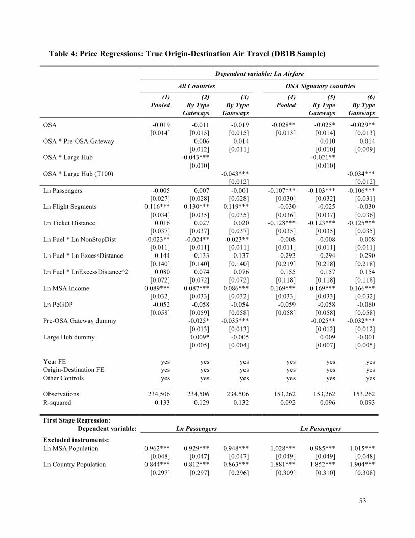
Agreements on model variables. OSAs lead to a 2-4 percent drop in average airfares (controlling
for trip characteristics). Prices are increasing in the number of segments, consistent with the
model, and decreasing in (instrumented) passengers flown, consistent with economies of route
density. The quantity of passengers flown doesn’t change for small cities, but grows 12.6 percent
for pre-OSA gateways and 11 percent for large hub cities capable of accepting international
traffic. Consumers have a strong preference for direct flights, as doubling the number of flight
segments has a demand effect equivalent to raising prices by 40 percent. Finally, OSAs generate
a 2.5 percent reduction in the number of segments a passenger flies, but only on those cities
6
where new direct connections occur. Passenger growth itself further reduces the number of
segments flown. Increased directness caused by OSAs implies a reduction in the U.S. exit points
used by passengers from large cities in their travels abroad. On average, passengers from pre-
OSA gateways and from large hubs reduce by 5 to 7 percent the number of exit points they route
through before leaving the U.S..
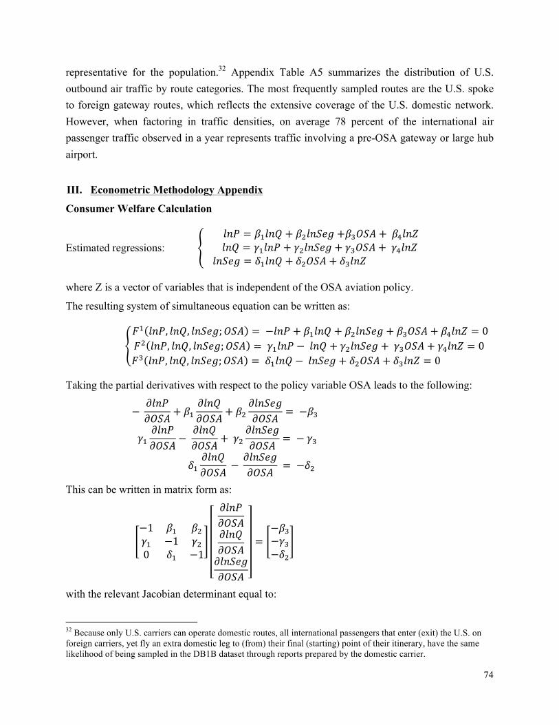
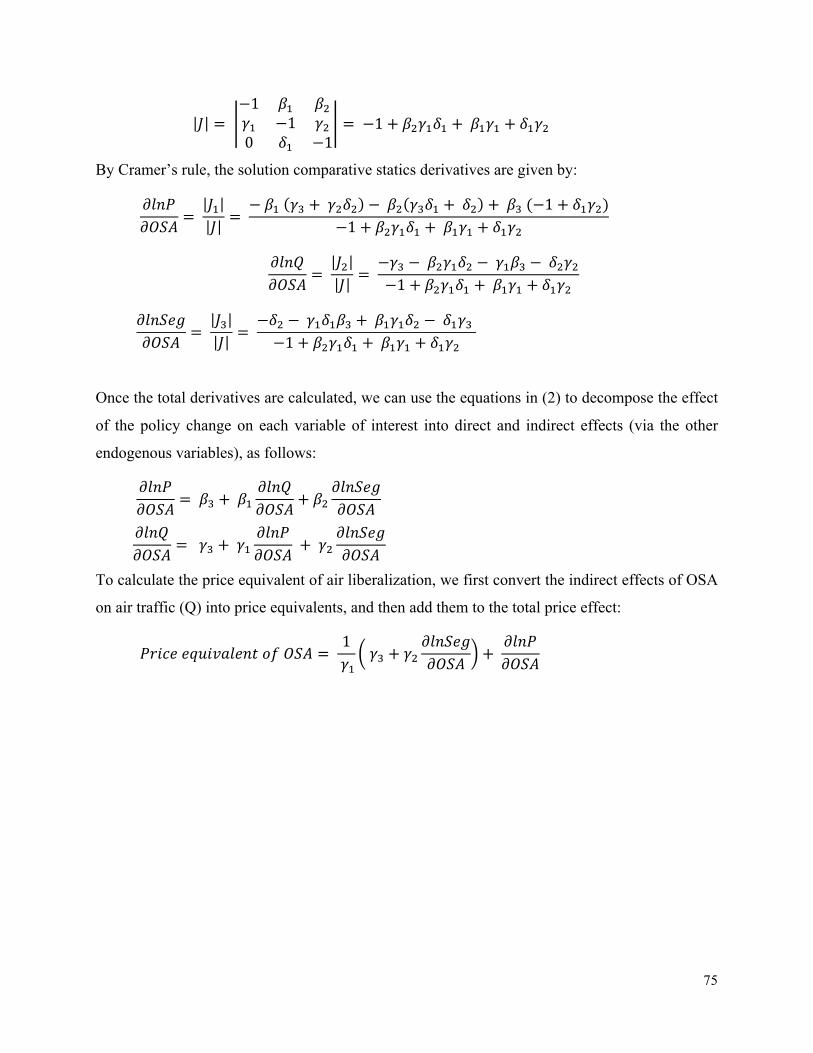
To conclude the paper we combine these partial derivatives in a system of equations to
compute the total derivative of quantities, respectively of (quality-adjusted) prices, with respect
to OSAs. The results show profound differences in effects across cities, which depend on the
extent to which liberalization relaxed the constraints facing each market. At the low end,
liberalization increases quantities in small spoke cities by 6.8 percent and lowers quality-adjusted
prices by 4.6 percent. At the high end, liberalization increases quantities in cities with new direct
connections by 23.7 percent and reduces quality-adjusted prices by 15.3 percent. A population-
weighted average across city types shows an aggregate decline in quality-adjusted prices of 8.8
percent.
The paper is organized as follows. We proceed with a brief literature review in the next
section, followed in Section 3 by a description of the liberalization process in international air
transport services. Section 4 describes the theoretical model and derives the main model
predictions to be examined empirically. Section 5 presents the data sources while the empirical
analysis and welfare calculation are discussed in section 6. Section 7 concludes.
2. Related Literature.
In this section we discuss the relevant theoretical and empirical literatures to which our
paper contributes. Our model is closely related to work on hub-and-spoke network formation,
and to models of Bertrand-Edgeworth price competition.
In the wake of the US domestic airline deregulation, many authors explored models of
hub-and-spoke networks (e.g. Caves et al., 1984; Bailey et al., 1985; Berry, 1990; Brueckner and
Spiller, 1991; Brueckner et al., 1992; Brueckner, 2004). These models usually focus on
economies of route density and/or consumer preferences for direct flights, and feature quantity
competition between firms who are free to choose the network structure. Some authors, notably
Hendricks et al. (1997, 1999), argue that price-setting competition is a more appropriate
environment for the airline industry. They focus on the difficulty of sustaining entry by multiple
7
carriers when those carriers first establish networks and then compete in prices. Models such as
Aguirregabiria and Ho (2010, 2012) feature differentiated products price-competition, which
allow multiple firms to compete in equilibrium because consumers differ in their taste for
particular carriers.
Like several of these papers, our model features endogenous carrier entry and network
formation, and allows carriers to be differentiated by type (direct, indirect flights) but otherwise
homogeneous within that type. Unlike the earlier work we sustain entry of multiple carriers of
each type within a price setting game by assuming the existence of capacity constraints and
uncertain demand. This has two additional merits. One, the model predicts empirically relevant
facts: unused capacity and price dispersion, both across firms as well as within a firm’s own
ticket offerings. Two, we can aggregate carrier ticket offerings into a tractable average price
function that allows us to calculate the welfare change after liberalization without estimating
consumers’ “brand loyalty” associated with entering/exiting carriers. This feature is especially
important when considering the large number of routes we analyze, and the prevalence of multi-
segment tickets offered by frequently changing combinations of multiple carriers.
Our modeling approach to capacity constrained price competition differs in several key
ways from standard Bertrand-Edgeworth competition (e.g., Kreps and Schienckman, 1983;
Osborne and Pitchik, 1986; Allen and Helliwig, 1986; Deneckere and Kovenock, 1996). The
Bertrand-Edgeworth model is typically formulated as a two-stage game in which firms first
choose costly capacity, which is observable, and then compete via prices over known demand.
Each firm has a constant per unit cost for production up to their respective capacity constraint,
and each firm chooses a single price. Demand is efficiently rationed.7 This can be thought of as a
situation in which the consumers, each with unit demand for the good and heterogeneous
reservation values, form an ordered queue that is decreasing with respect to the consumers’
reservation values. Consumers buy from the lowest priced firm up to the point that the lowest
price firm exhausts its capacity, then move on to the second lowest price firm and so on.
Our approach, which builds upon Prescott (1975), Eden (1990) and Dana (1999), is a
variation of the Bertrand-Edgeworth game. It features (i) intra-firm price dispersion, (ii) demand
uncertainty, and (iii) random rationing, meaning that the consumer queue is random, not ordered.
7 For an exception, see Davidson and Deneckere (1986) who use random rationing.
8
The first two distinctions, allowing each firm to sell tickets on a given route at multiple prices
and uncertain demand, are clearly critical features of our airline industry application.8
Reynolds and Wilson (2000) and Lepore (2012)9 also examine demand uncertainty in the
Bertrand-Edgeworth model,10 but the information structure there differs from our framework.
Uncertain demand is modeled as a three-stage game: capacity choice, realization of the state of
the demand, and then price competition. In our framework, demand is not realized until after the
firms have chosen price-quantity schedules. Combining this information structure with intra-firm
price dispersion and random rationing, we can summarize our game as follows: (i) carriers enter
and set capacity; (ii) carriers simultaneously choose price-quantity schedules that specify the
quantity of tickets to be sold at each price, (iii) heterogeneous consumers form a queue in which
the order of reservation values is random and the length of the queue is random, (iv) consumers
buy first tickets available at the lowest effective (quality-adjusted) price, regardless of carriers;
(v) ex-post, carriers have unsold tickets and face a capacity cost for holding them.
We also contribute to an empirical literature on airline deregulation. Liberalization of
international aviation markets follows earlier deregulation of U.S. domestic markets. Studies of
the U.S. domestic airline industry have shown that the inability of airlines to compete in prices
caused them to invest in service enhancements (Borenstein and Rose, 1998). Limitations in route
and capacity choices increased operating costs by restraining airlines' ability to optimize their
network structure, size and traffic density (Baltagi et. al, 1995).
The liberalization of international passenger aviation services has been the focus of few
recent studies.11 Several studies employ the same datasets that we use but very different sample
cuts in order to investigate the price effects of the inter-airline strategic alliances (Brueckner and
Whalen, 2000; Brueckner, 2003; Whalen, 2007; Bilotkach, 2007). These studies find that airline
alliances reduce airfares, which is consistent with our price results as OSAs facilitate the
8 This is a simplification of the dynamic problem that carriers face in pricing tickets, but as shown by Escobari and Gan (2007) this simplification appears to fit well with the airline industry. For more on the airline’s dynamic pricing problem, see the surveys in McAfee and te Velde (2006) and Aviv et al. (2012). Recent examples of this dynamic pricing problem include Wright et al. (2010), Deneckere and Peck (2012), Gallego and Hu (2014). 9 Issues regarding demand uncertainty and production flexibility also feature prominently in the operations management literature. See for example Anupindi and Jiang (2008). 10 Hu (2010) and Barla and Constantatos (2005) examine demand uncertainty in the context of hub-and-spoke network formation followed by quantity-setting competition. However, as in Reynolds and Wilson (2000) and Lepore (2012), the state of demand is realized prior to the final stage market competition subgame. 11 Apart from passenger aviation, Micco and Serebrisky (2006) focus on air cargo, often carried in the holds of passenger aircraft. They estimate that OSAs lowered air cargo freight rates for US imports by 9 percent.
9
formation of airline alliances.12 We do not explicitly treat alliances but instead focus on features
of agreements previously unexplored: route and capacity restrictions.
Piermartini and Rousova (2013) use a 2005 cross-section sample of worldwide country-
pairs to estimate the impact of air services liberalization on the bilateral volume of air passenger
flows. They estimate that OSAs increase traffic by 5 percent. Whalen (2007) uses similar data to
ours but a substantially different sample. He finds that OSAs increase airfares and have no effect
on passenger volumes once controlling for market competition and strategic alliances. Winston
and Yan (2015) examine the impact of liberalization on fares and passengers for a subset of
heavily trafficked international aviation routes, employing average fare data reported to IATA
from 2005 to 2009. They employ a difference-in-differences estimation method at the country
level for short run estimates, and employ cross-country variation for identification of long run
estimates. They find very large (approximately 50 percent) reductions in average fares.
We differ from these earlier studies in three respects. One, we tie our estimates closely to
an explicit model of the mechanisms through which OSAs liberalize markets. We demonstrate
the importance of these mechanisms in the data, and provide consumer welfare estimates that
decompose the channels of response. Two, by using a comprehensive set of ticket data that
includes connecting flights, we can demonstrate the differential impact of liberalization across
different city types, as suggested by the model. Three, we have a longer panel which allows us to
employ difference-in-differences estimates to identify within city-pair changes in price, quantity,
and directness (i.e., flight connections) for a large number of agreements. This prevents
heterogeneity across city-pairs from affecting our results.
3. Liberalization in International Air Transport Services
Historically, the provision of international air services has been restricted by a complex web
of regulations set on a bilateral basis.13 A standard bilateral aviation agreement specifies a
limited set of gateway points/airports that can be serviced by a restricted number of designated
airlines (typically one or two carriers from each country). It also delineates the traffic rights
granted to operating carriers, the capacity that can be supplied in each origin-destination city pair 12 These results differ from ours substantially in terms of theoretical approach and data analysis. 13 Efforts to set a multilateral regulatory framework go back to the Chicago Convention of 1944 when the International Civil Aviation Organization (ICAO) was established under the auspices of the UN. Apart from safety and technical rules, the Convention failed to reach common grounds. Bilateral agreements became the norm and passenger aviation remains outside the General Agreement on Trade in Services (GATS).
10
(with exact rules for sharing capacity), and the air fares to be charged on each route (with both
countries’ approval required before they can enter into effect). The prices agreed upon in the
agreements frequently correspond to the fixed rates set by IATA during periodic airfare
conferences (Doganis, 2006).14
As an example, the US-China Aviation Treaty (1980) restricts market access to two
designated airlines per country, who can operate at most two round-trip flights per week, each on
routes connecting four U.S. points (New York, San Francisco, Los Angeles, Honolulu) to two
Chinese cities (Shanghai, Beijing). Tokyo is the only third country location from where service
to either country's designated airports can be operated. Prices charged on all routes must be
submitted to government authorities two months in advance for double approval. In addition,
both countries can take ‘appropriate’ action to ensure that traffic is ‘reasonably balanced’ and
mutually beneficial to all designated airlines.
In 1980, the United States passed the International Air Transportation Competition Act,
which set the stage for opening international aviation markets. The liberalization efforts debuted
with the renegotiation of many U.S. bilateral aviation agreements during the 1980s – the “open
markets” phase. The main focus of these treaty renewals was to relax market access and capacity
restrictions by extending the number of designated airlines, the pre-defined points of service, and
the flight frequencies. Some agreements also granted a partial relaxation of pricing provisions
and beyond traffic rights (i.e., the right to fly passengers between two pre-approved foreign
points on the way to/from a carrier's home country).
Between 1992 and 2013 the U.S. signed 106 bilateral Open Skies Agreements.15 These
agreements grant unlimited market access to any carrier for service between any two points in
the signatory countries, full flexibility in setting prices, unconstrained capacity choice and flight
frequencies, unlimited access to third country markets, and a commitment to approve inter-
airline commercial agreements (e.g., code-share, strategic alliances). The timing and complete
list of partner countries is reported in the Appendix Table A1. Apart from the completely
liberalized intra-EU aviation market, U.S. efforts to deregulate international aviation in this
14 IATA (International Air Transport Association) is the trade association of international airlines and one of its main tasks has been to fix prices on most international city-pair routes. Because IATA prices have to be agreed upon by all member airlines, they tend to be high enough to cover the costs of the least efficient carrier (Brueckner, 2003). 15 In this period, the US also signed a small number of partial liberalization agreements that served in several cases as a short transitory stage before signing a full OSA. We address these partial liberalization efforts in our empirical work. Of the 106 agreements, 94 occurred within the time frame covered by our data.
11
period are atypical. While some air service agreements have been amended to relax regulatory
provisions, overall the global aviation market remains fairly closed to trade.16
4. Model
We study a three-stage model. In the first stage carriers enter and form international
networks. In the second stage they set capacities and price-quantity schedules, after which
uncertain demand is realized and tickets are purchased. We begin by describing the final stage
price-capacity competition for an arbitrary international route 𝑗, with 𝑛! carriers providing direct
service and 𝑛! carriers providing indirect service (where indirect service involves a single
stop).17 We then consider the network formation stage, and describe the equilibrium.
Our characterization of demand has three critical elements: a preference for directness,
random rationing, and uncertain total demand. We assume that consumers prefer a direct flight to
an indirect flight as long as the price 𝑝!of the indirect flight is equal or larger than the fraction
𝛼 ∈ (0,1) of the price of the direct flight 𝑝!, i.e., 𝛼𝑝! ≤ 𝑝!. If 𝛼𝑝! > 𝑝!, then the indirect flight
is preferred. It will be convenient to define the ‘effective’ price of a ticket, where for an indirect
ticket with price 𝑝! the effective price is 𝑝 ≡ !!
! and for a direct ticket with price 𝑝! the effective
price is 𝑝 ≡ 𝑝!.
We assume random (also known as proportional) rationing. This is consistent with
heterogeneous consumers, each having unit demand and differing reservation prices, randomly
queuing and purchasing the lowest effective price tickets first, subject to availability. In addition
to the random ordering of the heterogeneous consumers in the queue, there is uncertainty
regarding the number of consumers/length of the queue, and this uncertainty is not resolved until
after carriers make their price-capacity choices.
Formally, the demand uncertainty takes the form 𝑒𝐷(𝑝) where 𝑒 is the random state of
demand that is distributed according to the distribution function 𝐹(𝑒) which is continuously
differentiable with 𝐹! 𝑒 > 0 and 𝐹!! 𝑒 ≤ 0 for 𝑒 ∈ [0,1] and 𝐹 0 = 0. We assume that
demand is twice continuously differentiable, with 𝐷′ 𝑝 < 0 and 𝐷 𝑝 + 𝑝𝐷′ 𝑝 < 0 for all
𝑝 ∈ 0,𝑝 , and that there exists a finite price 𝑝 = inf{𝑝|𝐷 𝑝 = 0}. 16 Piermartini and Rousova (2013) provide a comprehensive description of 2300 bilateral aviation treaties in force in 2005, concluding that 70 percent of bilateral agreements worldwide are still highly restrictive. 17 We ignore directional flow issues, impose the restriction that prices must be the same in each direction, and focus on the total quantity of round-trip travel demanded on a given route at a given effective price.
12
In the final stage of the price-capacity competition, carriers choose both a total capacity
and a ticket price for each unit of available capacity. Allocating capacity to a route is costly, and
we assume that this takes the form of a constant per-unit cost of 𝜆! for a direct international
flight. In the case of indirect flights, there is only one stop and the capacity cost of this
connecting flight is 𝜆! . Thus, the total capacity cost for an indirect flight is 𝜆! + 𝜆! . To simplify
the expressions, we assume that up to the capacity constraint, the per-unit cost of utilizing
existing capacity is zero. Although it is straightforward to relax this assumption, many of the
costs of providing service on a route, such as fuel burn, flight crew, etc., depend primarily on the
capacity choice.
In order to ensure the existence of an equilibrium with strictly positive capacity choices,
we assume that 𝑝 > !!!!!!
, where 𝑝 = inf{𝑝|𝐷 𝑝 = 0}. For the case of constant elasticity
demand, as is used in the empirical specification, this assumption regarding the choke price
corresponds to 𝐷 𝑝 = 𝐴 𝑝 !! > 0 for all 𝑝 ≤ 𝑝 and 𝐷 𝑝 = 0 otherwise.
The model of oligopoly price-capacity competition that we have described to this point
extends Dana (1999) by allowing firms to be heterogeneous with respect to directness (which
implies heterogeneous costs) and for consumers to have a preference for directness. As Dana
(1999) shows, uncertain demand combined with capacity costs implies that equilibrium involves
non-degenerate price-quantity schedules, i.e. price dispersion, in which ticket prices are
increasing in quantities sold.
To understand why, consider the impact that demand uncertainty has on the probability of
selling a marginal ticket. The minimum price is set to guarantee that at least one ticket sells even
in the lowest state of demand. After this point, the probability of making a sale decreases as the
cumulative market quantity of ticket sales increases. Then, because carriers require higher
marginal revenue to hold inventories of seats that sell with lower probability (and have the same
capacity costs), it follows that each carrier has a strict incentive to sell tickets at a range of prices
rather than at a single price.
Formally, let 𝑞!(𝑝) denote carrier 𝑖’s marginal quantity schedule, where 𝑄! 𝑝 =
𝑞!(𝑟)𝑑𝑟!! denotes the total number of tickets that carrier 𝑖 prices at or below 𝑝. Note that carrier
𝑖’s total capacity costs are 𝑄! 𝑝 𝜆! if carrier 𝑖 is a direct carrier and 𝑄! 𝑝 (𝜆! + 𝜆!) if carrier 𝑖
is an indirect carrier.
13
To calculate carrier 𝑖’s expected revenue, note that 𝑝 is the highest effective price at
which a ticket has sold, 𝑒 is the state of demand, and the market marginal quantity schedule is
given by 𝑞 𝑝 = 𝑞!(𝑝)! . Then under random rationing, the residual demand is calculated as:
𝑒𝐷 𝑝 1− !(!)!"(!)
!! 𝑑𝑟 (1)
If 𝑝 < 𝑝 is the highest effective price at which a ticket sells when 𝑒 is the state of demand and
when 𝑞 ⋅ is the market marginal quantity schedule, then we know that residual demand is equal
to zero at effective price 𝑝. That is:
𝑒𝐷 𝑝 1− !(!)!"(!)
!! 𝑑𝑟 = 0 (2)
We can define the ‘market clearing’ demand shock 𝑒(𝑝, 𝑞) as:
𝑒(𝑝, 𝑞) = !(!)!(!)
!! 𝑑𝑟 (3)
Because the demand shock 𝑒 is distributed according to 𝐹(⋅), the probability that a ticket priced
at 𝑝 sells is 1− 𝐹 𝑒 𝑝, 𝑞 . Thus, the profit functional for carrier 𝑖 offering a direct flight on the
To solve for the equilibrium price-quantity schedules, we formulate each carrier’s profit
maximization problem as an optimal control problem. In this environment the Hamiltonian is not
concave and so the (Pontryagin) Maximum Principle only provides a necessary condition for
14
optimization. However, by using the Extension Principle, it is possible to solve for the final-stage
local equilibrium price-quantity schedules which are given in Theorem 1 in the next section. 18
Given the form of final stage price-capacity competition, we now move back to the first-
stage international-hub formation game. There are two countries, a domestic country 𝐴 and a
foreign country 𝐵, and two types of cities: (i) gateway cities that may serve as an international
hub both pre- and post-OSA and (ii) non-gateway cities that are domestic hubs for one or more
domestic carriers and are large enough that they may profitably serve as an international hub
post-OSA. Country 𝐴 is a large country with an arbitrary (but strictly positive) number of
gateway cities and an arbitrary (but strictly positive) number of non-gateway cities. For
simplicity, we will assume that country 𝐵 has a single gateway city and no non-gateway cities.
In the first stage of the game, we take the domestic network as given and each country 𝐴
carrier chooses whether to form an international hub at each of its (exogenously given) country 𝐴
domestic hubs. Each country 𝐵 carrier chooses whether or not to form an international hub at the
country 𝐵 gateway city. For simplicity, we assume that any country 𝐴 domestic hub may offer
direct service to each of the other country 𝐴 cities.
In the baseline model we assume that the cost of forming and maintaining an
international hub is proportional to a carrier’s international capacity choice, which is made in the
second stage of the game. Note that this assumption makes the first-stage international-hub
formation game trivial, and in equilibrium each carrier will form an international hub in each city
where it has the ability to do so. However, it is straightforward to extend the baseline model to
account for economies of scale and economies of traffic density issues by assuming a fixed cost
of international hub formation, as in Hendricks et al. (1997, 1999) and similar to Aguirregabiria
and Ho (2010, 2012).
In the equilibrium of the international hub-formation stage with fixed entry costs, the
number of carriers forming international hubs decreases relative to the case with no fixed cost.
Each carrier only forms an international hub in a city if (a) the total traffic, direct and indirect,
through the hub covers the fixed cost of forming the hub and (b) there are no alternative
international hub configurations, in which indirect flights may be rerouted through alternative
18 For more on this approach see Krotov (1996). This method involves mapping the original problem into a well-behaved equivalent extension, solving the extended version of the problem, and then mapping the solution back into the original problem.
15
hubs that are more profitable. In the following section, we examine an extension that accounts
for these issues.
4.1 Equilibrium
We focus on subgame perfect equilibria that are symmetric in that the final-stage local
equilibrium price-quantity schedules are symmetric within carrier type, and all equilibrium price-
quantity schedules have the same price support for a given route. That is, all direct carriers offer
the same price-quantity schedule, which differs from the indirect carriers, all of whom offer the
same price-quantity schedule.
We begin in the final stage price-quantity schedule setting subgame and then move back
through the game tree to the international network formation stage. Our setup simplifies the
network stage in two ways. One, the assumption that capacity costs are linear allows us to solve
for the equilibrium price-quantity schedule on each route in isolation. Two, it is clearly
suboptimal for a carrier with the ability to offer direct service to offer both direct and indirect
service for the same city pair.19 To economize on notation we will henceforth use 𝑝 instead of 𝑝
to denote the effective price.
Theorem 1 There exists a symmetric final-stage local equilibrium that is described as follows.
1. If , then let be defined as:
The lower bound of the support of the prices, , solves . Each direct carrier’s
equilibrium price-quantity schedule is, for 𝑝 ∈ [𝑝,𝑝):
𝑞! 𝑝 =𝐷(𝑝)𝑛
−𝑦∗(𝑝)𝐹′(𝐹!!(1− 𝑦∗(𝑝)))
−𝑛!𝐷′(𝑝)
𝐹′(𝐹!!(1− 𝑦∗(𝑝)))𝑝𝐷(𝑝)𝜆! + 𝜆!
𝛼 − 𝜆!
19 Such a carrier could increase its profits by shifting all indirect flights to direct flights which would decrease costs and increase the prices that consumers are willing to pay.
0>In )(* py
( )
( ) 1
11
1*
)(
)()(
11
)()(=)(
−
−−
ʹ⎟⎟⎠
⎞⎜⎜⎝
⎛⎟⎠
⎞⎜⎝
⎛ ++
−−⎥
⎦
⎤⎢⎣
⎡+ ∫
nn
nCDIDD
p
pnn
CD
ppD
drrrDrDnn
nppDpDp
ppy α
λλλ
αλλ
p 1=)(* py
16
and each direct carrier places a mass point at of size:
For indirect carriers, the equilibrium price-quantity schedule is:
𝑞! 𝑝 = 𝑞! 𝑝 +𝐷′(𝑝)
𝐹′(𝐹!!(1− 𝑦∗(𝑝)))𝑝𝐷(𝑝)𝜆! + 𝜆!
𝛼 − 𝜆!
2. If , then let be defined as:
The lower bound of the support of the prices, , solves . Each direct carrier’s
equilibrium price-quantity pair is, for :
The proof of Theorem 1 is given in the Theory Appendix 1A. In solving for the equilibrium
price-quantity schedules {𝑞! 𝑝 }! , the carriers’ optimization problems depend critically on the
the probability that a ticket with effective price 𝑝 sells, which is given by 1− 𝐹 𝑒 𝑝, 𝑞 . This
probability depends on the total market price-quantity schedule, 𝑞 𝑝 = 𝑞!(𝑝)! , via the
‘market-clearing’ shock 𝑒 𝑝, 𝑞 .
The 𝑦∗(𝑝) expression in Theorem 1 provides the probability 1− 𝐹 𝑒 𝑝, 𝑞 at the
equilibrium total market price-quantity schedule 𝑞 𝑝 . Then given the equilibrium probability of
making a sale as a function of the price 𝑦∗(𝑝), the equilibrium price-quantity schedules for the
direct and indirect carriers may be written in terms of 𝑦∗(𝑝), where 𝑦∗ 𝑝 denotes the equation
of motion for 𝑦∗(𝑝) as the effective price 𝑝 varies over the price support. Because 𝑞 𝑝 is the
market marginal quantity schedule, the cumulative market quantity of tickets that are sold at or
below an effective price of 𝑝 is given by 𝑄 𝑝 = 𝑞(𝑟)𝑑𝑟!! .
Thus, the model may be summarized as follows. A demand shock 𝑒 determines the length
of the randomly ordered queue of customers with heterogeneous unit demands. The customers in
p
⎟⎟⎠
⎞⎜⎜⎝
⎛⎟⎟⎠
⎞⎜⎜⎝
⎛ +−−⎟⎟
⎠
⎞⎜⎜⎝
⎛−Δ −−
αλλλ
pF
pF
np CDD
D
D 111=)( 11
0=In )(* py
( )
( ) 1
11
1*
)(
)()(
1)()(=)(
−
−− ʹ
−−⎥
⎦
⎤⎢⎣
⎡ ∫nn
nD
p
pnn
D
ppD
drrrDrD
nn
ppDpDp
ppy
λλ
p 1=)(* py
],[ ppp∈
( ) ⎟⎟⎠
⎞⎜⎜⎝
⎛
−ʹ−− )))((1(
)(=)( *1
*)(
pyFFpypq n
pDD !
17
the queue buy first the lowest effectively priced tickets, and then continue moving up the
carriers’ price-quantity schedules until either the demand or the supply of tickets is exhausted. If
𝑝 is the highest effective price at which a ticket sells, then the total quantity of tickets that are
sold in the market is 𝑄 𝑝 .
Note that as tickets sell at multiple prices the cumulative market quantity of tickets sold is
determined by the maximum price in the market. However, in matching the theory with the
empirics, it will be convenient to write the market quantity as a function of the average price
instead of the maximum price. Towards that end, let 𝜌(𝑒, 𝑞) denote the maximum price at which
a ticket sells. Making a slight abuse of terminology, hereafter we refer to it as the ‘market-
clearing’ price. This price is a function of both the random length of the queue, (i.e. the demand
shock 𝑒), and the market price-quantity schedule, 𝑞, so 𝜌(𝑒, 𝑞) is implicitly defined by
𝑒 𝜌 𝑒, 𝑞 , 𝑞 = 𝑒.
For a given 𝑞 and 𝑒, the total quantity of tickets that are sold is 𝑄 𝑒 ≡ 𝑄 𝜌(𝑒, 𝑞) . If
the total quantity of tickets sold is Q, then the average market price as a function of 𝑄, denoted
𝑝!"#(𝑄), solves 𝑄!!(𝑄)𝐷 𝑝!"#(𝑄) = 𝑄. This implies:
𝑝!"#(𝑄) = 𝐷!! !!!!(!)
(6)
To fix ideas, consider the special case of CES demand that will be used in the empirical section.
We parameterize the demand for international travel on a city pair at the effective price 𝑝 as
𝐷 𝑝 = 𝐴𝑝!! (7)
where 𝐴 corresponds to the population of potential international travelers on the given route, and
𝜖 denotes the constant elasticity of demand. For the sake of this example, we will also assume
that the demand shocks are uniformly distributed on [0,1]. From Theorem 1 we have that, for
For the case of CES demand, where the expected profit functions are linear with respect to the
population 𝐴, the entry conditions can be characterized by: 𝑛! = 𝑛! if, for each domestic carrier
22
with the ability to form an international hub, !!!"
!< 𝜋!(𝑞 𝑛!)− 𝜋!(𝑞 𝑛! − 1); or 𝑛! is the
largest value 𝑛! < 𝑛!, such that 𝜋!(𝑞 𝑛! + 1)− 𝜋!(𝑞 𝑛!) <!!!"
!< 𝜋!(𝑞 𝑛!)− 𝜋!(𝑞 𝑛! −
1), where population 𝐴 is normalized to one. It follows immediately that the number of direct
carriers is proportional to the relevant population on the route.
4.4 Model Estimation
We examine how international passenger aviation changes in the wake of trade
liberalization efforts, focusing on change along three dimensions. First, we use a difference-in-
differences methodology to compare growth in passenger traffic pre/post liberalization to growth
in the same period for non-liberalization countries. Second, we decompose aggregate changes in
international air traffic into growth in number of city-pair routes (extensive margin) and growth
in average passengers per route (intensive margin). We also evaluate reallocations of carrier
capacity across routes. The decomposition provides insights into key model mechanisms and the
role of route restrictions in pre-OSA regulation. Third, we estimate the partial effects of
liberalization on the price, quantity and quality (directness) of passenger aviation, and examine
whether these effects are asymmetric across gateway and non-gateway cities, as predicted by the
theory. Finally, we combine these estimates to calculate the total change in (quality-adjusted)
prices after OSAs in order to assess the consumer welfare gains from air services liberalization.
5. Data Sources and Description
We draw on two rich datasets that cover international travel to and from the United States
over the period 1993-2008. The Databank 1B (DB1B) Origin and Destination Passenger Survey
represents a 10 percent sample of airline tickets drawn from airport-pair routes with at least one
end-point in the U.S. Each airline ticket recorded in the dataset contains information on the
complete trip itinerary including airports, air carriers marketing the ticket and operating each
flight segment, the total air fare, distance traveled split by flight segments, ticket class type, as
well as other segment level flight characteristics.
One limitation of the DB1B data is that the foreign carriers who are not part of immunity
alliances are not required to file ticket sales information to the U.S. Department of
23
Transportation.20 However, this is less of an issue for U.S. outbound tickets as compared to
inbound ones. Tickets whose first segment originates in the U.S. are more likely to be sold by
U.S. carriers and therefore more likely to appear in the data. For this reason, in this paper, we
focus on U.S. outbound economy-class tickets. We employ additional filters to prepare the data
sample, which are described in the Data Appendix. The resulting sample includes 21,067 origin-
destination city pairs, with an average of 11 observations per pair. The summary statistics for the
variables of interest are provided in the Appendix Table A4.
We augment the empirical analysis with an alternative dataset that offers complete
coverage of all U.S. international passenger traffic. The T100 International Segment database
provides information on capacity and air traffic volumes on all U.S. non-stop international flight
segments (defined at airport-pair level), distinguished by the direction of travel, and operated by
both domestic and foreign air carriers. The data is collected at monthly frequencies and reports
for each carrier-route pair the number of departures scheduled and operated, seats supplied,
onboard passengers, segment distance and airborne time.21 The disadvantage of the T-100 data is
two-fold. They do not include pricing information, and they do not provide details on complete
origin-destination itineraries, but rather report only the flight segments that cross the US border.
Accordingly, the T100 data are best for describing changes in total passengers exiting the
US, the number of distinct exit points out of the US, and the capacity allocated to those exit
points. This makes it ideal for evaluating model mechanisms related to route restrictions and
capacity reallocation. The DB1B data are best suited for describing prices and routing structures
at the level of true origin-destination city pairs, especially when indirect tickets have a significant
market share. This makes it ideally suited for evaluating changes in consumer welfare.
Table 1 summarizes regional growth in passenger traffic on non-stop segments, and
regional growth in the share of traffic covered by OSAs during the sample period 1993-2008.
Figure 1 shows the annual time series aggregated over regions. By any measure of industry
performance - passenger volumes, number of non-stop international routes or annual departures
20 Immunity alliances represent strategic alliances between domestic and foreign airlines with granted antitrust immunity from the U.S. Department of Transportation. Immunity grants allow carriers to behave as if they were merged, cooperating in setting prices and capacity on all joint international route to and from the U.S. 21 However, the T100 Segment data does not easily match to the true Origin and Destination Passenger data, since passengers with very different start and end point itineraries get lumped together in a single observation in the T100 Segment dataset if their cross-border flight segment is the same. Unlike goods, which feature a one-to-one relation between a product and its producer, international air travel often involves the service of more than one airline. This is why firm- and product-level air travel datasets are imperfectly compatible.
24
performed (unreported) - international air traffic has grown rapidly during this liberalization
period. By 2007, 61 percent of the total U.S. international air passenger traffic passed through a
foreign gateway airport located in an Open Skies country.
6. Econometric Analysis
6.1 Growth of Passengers and Routes: T100 Data
We begin by examining traffic growth using the T-100 International segment data. We
observe passenger traffic for every carrier and every non-stop cross-border city-pair route. Total
air passenger traffic between the United States and destination country d in year t is the sum of
traffic across all non-stop origin-destination routes and carriers offering service. We decompose
the total annual U.S. outbound traffic to country d, Qdt, into an intensive and extensive margin
using the simplest approach. We count the number of direct connection city-pair aviation routes
offered in a given year, Ndt, and then determine the average passenger volume per route:
𝑄!" = 𝑄!"# = 𝑁!"! ∗ 𝑄!" (14)
To estimate the impact of liberalization on air passenger transport, we rely on the time
series dimension of the T100 International Segment data. Our identification strategy compares
the change in passenger volumes within a country pair before and after the introduction of the
Open Skies Agreements, with the corresponding value calculated for countries that maintain
restrictive aviation policies (control group). In using this difference-in-differences estimation
method we consider the following regression model:
where d and t index the foreign country and year respectively, and Z ∈ {Qdt, Ndt, 𝑄!"} takes in
turn each variable. The variable of interest OSAdt is an indicator variable that equals 1 for all the
years when an Open Skies Agreement is in effect between the U.S. and country d. We also
control for the income per capita Y/L, and the population size L of destination country d. X
denotes a vector of additional control variables, including an indicator variable Partial
Liberalization (i.e., non-OSA countries with more flexible air transport agreements), a country-
specific Visa Waiver Program (VWP) indicator and its interaction with a September 11 indicator
25
variable to capture any differential responses to the tightened security post 9/11 (Neiman and
Swagel, 2009). We also control for linear trends specific to selected world regions (e.g.,
Caribbean countries, countries affected by the Asian crisis), as well as for country and year fixed
effects. Since our data consists of aggregate U.S. bilateral flows, the year effects eliminate any
time-varying changes that are common to all U.S. aviation routes, including changes in input
prices or technology, or secular changes in aviation demand.
Endogeneity of Open Skies Agreements
One complication in policy evaluation comes from the potential endogeneity between the
change in policy and the outcome variable(s) of interest. In our case, a primary concern is that
some omitted variable affects the scale or expected future growth of aviation traffic with country
d, and this omitted variable is correlated with the likelihood and/or timing of an Open Skies
Agreement. Countries differ substantially in size and income, the quality of aviation
infrastructure, the dependence on aviation for trade, migration, or tourism, and the strength or
political connections of their domestic airlines. The US may be more likely to sign agreements,
or sign them earlier, when the benefits of signing are greater and the political opposition to
signing is less.
Using a probit model, Appendix Table A2 investigates the likelihood of signing OSAs
among the countries in our sample. We use information on the levels and growth rates of various
country characteristics such as population, GDP, GDP per capita, exports and geographic
distance. None of these country characteristics have a statistically significant effect on the
likelihood of signing OSAs (though if we enter a “high income” indicator with no other controls
it is marginally significant). We also explore the characteristics of aviation routes prior to the
signing of agreements. We include the country’s number of departures worldwide, the total
number of international destinations (i.e., aviation routes), as well as the carrier concentration on
routes. Still, we find no significant effects on the probability of signing OSAs. In unreported
specifications, we also experiment with information on the restrictiveness of existing (pre-OSA)
air service agreements, including whether they included restrictions on routes, carriers, price
setting, or capacity restrictions. Of these, only the existence of capacity restrictions is (weakly)
correlated with early signing, and so we include the degree of partial liberalization as a control in
our main regressions.
26
Even if endogeneity were a concern, this problem is likely to be most severe in the cross-
section, as there are a host of difficult-to-control reasons for why Germany and Ghana differ in
the structure of their aviation markets, and in their returns to signing such agreements. Many
studies of services liberalization are limited to cross-section data, but we are able to employ a 16-
year panel dataset and use country fixed effects to exploit only within country time series
variation pre/post signing (in the regressions using DB1B data we employ even more stringent
fixed effects at city-pair level).
Countries that sign agreements at some point may be fundamentally different than
countries that do not sign agreements at any point. We can exploit our long time series and the
fact that a significant number of countries, i.e., 94 countries, have signed OSAs over our period
of study, 1992-2008. This only leaves the endogeneity of the timing of the agreements. As an
initial look at this problem, we inspect the dates when OSA agreements went in effect, which are
provided in the Appendix Table A1. What we see is that there is no clear pattern to the timing of
the agreements. After The Netherlands signs the first agreement in 1992, 8 OECD European
countries sign in 1995. But the rest of Europe is spread throughout the sample, with one country
signing in 1996, 1998, 1999, 2001, and then a final group in 2007. Many Latin American
countries sign in 1997, and other signings occur over the next 8 years. Similar partners are found
for East Asia, South Asia, Central Europe, and Africa. Table 1 reports the percentage of each
geographic region covered by OSAs at the start and end of our sample period, and again there is
no clear pattern. By 2008, all of OECD Europe is in, but other regions all have a mix of signers
and non-signers.
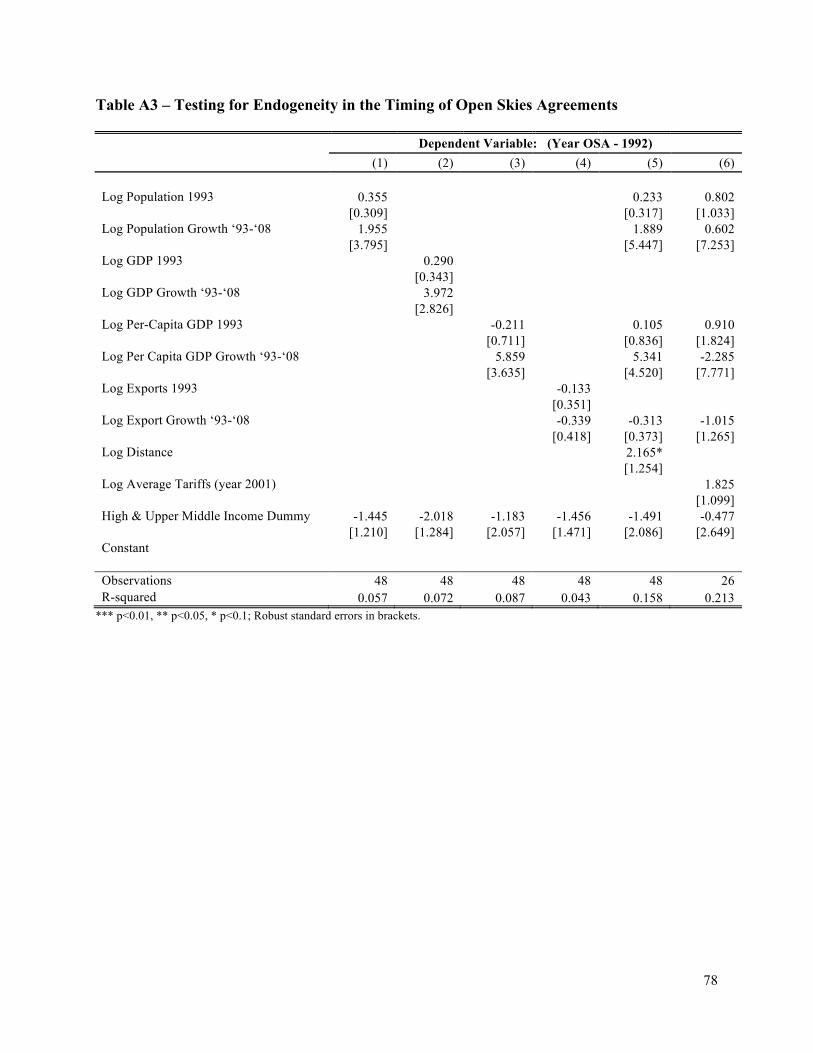
Using regression analysis, Appendix Table A3 examines the timing of OSA signing and
its correlation with country characteristics such as the levels and growth rates of population,
GDP, GDP per capita, exports, geographic distance and average tariffs. In unreported results we
also explore the characteristics of aviation routes prior to the signing of agreements. We include
the country’s number of departures worldwide, the total number of international destinations and
air carrier concentration on routes. None are statistically significant at conventional levels.
A final possibility is that there are changes in growth rates that happen to coincide with
signing OSAs. To rule this out we interact the OSA dummy with a vector of time dummies
corresponding to t-4 through t+5, where t is the year of signing. This enables us to see whether
aviation traffic was already growing prior to the OSA signing, or whether changes in growth
27
rates correspond to the date the agreements were signed. We return to this point in the results
discussion below.
Estimation Results
Panel A of Table 2 reports the regression model in equation (15) estimated using the
decomposition of international air traffic in equation (14). In Column 1 we see that countries
who liberalize their international aviation markets experience a 30.6 percent increase in
passenger traffic. The increase in aggregate volumes is explained in part by the net expansion of
international aviation routes. Countries that sign OSAs see a 17.4 percent faster growth in the
number of routes, as measured by a simple count (Column 2). Liberalization also affects the
average passenger growth per route, though the intensive margin effect is imprecisely estimated
(Column 3). Given the log-additive property of the components of the air traffic decomposition,
the coefficients on OSA in the total traffic regression will be equal to the coefficients from the
extensive and intensive margin regressions, respectively. We can then say that the extensive
margin accounts for (0.160/0.267) = 60 percent of the overall growth in the total air passenger
traffic.
The simple OSA indicator specification assumes that there is a one-time level change in
growth rates after signing the agreement. But the aviation industry may take time to adjust to
new policies, as carriers experiment with new markets and route networks, and consumers learn
about new travel opportunities. To account for this, we interact the OSA indicator with a vector
of time dummies corresponding to t-1 through t+5, where t is the year of signing. This enables us
to see whether increases in traffic growth accumulate over time.
Panel B of Table 2 reports the regression results. Two points emerge from these
estimates. First, for all three dependent variables (i.e., total traffic, extensive and intensive
margins) the impact of air services liberalization increases monotonically over time. Focusing on
the long run effects, we find that the growth of air passenger travel after five or more years since
an Open Skies Agreement is 60 percent. New routes account for half of the growth while the
remaining half is explained by the average passenger growth per route.
This approach also allows us to address any concern regarding the endogeneity of OSAs,
by which some excluded variable induces a change in growth rates, and this change in growth
rates induces the country to sign the agreement. We repeat the estimates, but interacting time
28
dummies from (t-4) to (t+5) to explore whether the change in growth occurred prior to signing.
We plot the coefficients in Figure 4.22 The plot makes clear that in the years prior to the signing
of Open Skies Agreements there are no statistically significant differences in the growth of air
transport between signers and non-signers, but that the growth rate after signing is significant.
For this to be driven by some factor other than the OSA it would have to be the case that the
potentially omitted variable actually changed in the same year as that when the OSA was signed.
Further, since we have 94 different signings over a 16-year period, this omitted variable would
have to coincidentally change at the same time as the OSA signing in every market, but in a
different year for every country. This seems unlikely.
In a further attempt to eliminate endogeneity concerns, we re-estimate all the regression
specifications from Table 2 using only the sample of OSA signatory countries. We define as
OSA signatory any country that signs an OSA during the period 1990-2013. The key advantage
of this subsample is that all countries included go through the liberalization process at one point
in time. So, this eliminates the concern that signatory countries might be different than non-
signatory countries in some unobserved characteristics that affect international air traffic. Now,
the only source of identification for the variable of interest, the OSA dummy, comes from the
timing of the agreement. Looking at the estimation results reported in Table 3, they are slightly
smaller in magnitude but very similar to the full sample results from Table 2. Countries that sign
OSA witness a 22.6 percent growth in air traffic relative to countries that haven’t liberalized their
market yet. Growth in new routes explains 72.5 percent of this effect, while the remaining 27.5 is
explained by the average growth in passengers per route (although this effect is not statistically
significant). The larger role played by the extensive margin is also observed in the long run
estimates reported in Panel B of Table 3. Overall, the estimates obtained from the sample of
OSA signatory countries reinforce all the findings from the full sample.
6.2 Entry and Exit: Carriers and Capacity
Our model suggests that Open Skies Agreements lead to two distinct kinds of entry / exit
patterns. Relaxing route and foreign carrier restrictions leads to an expansion of routes, as clearly 22 The data sample is an unbalanced panel and includes countries that sign OSAs throughout the sample period. To avoid the concern that the coefficients on the time dummies pre- versus post-OSA are affected by country composition, we expand the sample period to years 1990-2013 and keep in the sample only OSA signers that are observed at least 4 years prior to liberalization and 5 years post liberalization. This way the coefficients for the time dummies from (t-4) to (t+5) are identfied from the same set of OSA signatory countries.
29
shown in the last section, as well as an expansion of capacity and increased competition outside
of gateways. Does this expansion represent entirely new activity or is it a reallocation of capacity
and competition away from pre-OSA gateways to the new hub routes? In our model extension
with fixed entry costs (subsection 4.3), expanding the set of routes leads to exit from gateways
after signing. Domestic carriers who, pre-OSA, were forced to offer service through gateways to
attract international passengers into their hub routes can, post-OSA, offer direct service and
forego the fixed cost of establishing a gateway presence.
We examine these conjectures in the last two columns of Table 2 and Table 3,
respectively, as well as in Figure 5. In Tables 2 and 3 we measure capacity as the total number of
seats offered between the U.S. and country d, and we also measure the share of pre-OSA
gateways in the total number of seats offered. (Multiplying these measures together gives the
number of seats offered on pre-OSA gateways; adding the coefficients gives the change in those
seats after OSAs). In panel A of Table 3 we see that the average effect is a 23.6 percent rise in
total capacity post-OSA and a 4.3 percent reduction in the share of seats from pre-OSA
gateways. This implies that capacity outside the gateways rises faster than on pre-OSA gateways.
In Panel B of Table 3 we interact the OSA variable with a vector of time dummies to see
transition and long run effects. Five years after signing, post-OSA capacity rises by 39.4 percent,
and the share of pre-OSA gateways falls by 11.6 percent. If we compare the share of capacity on
the gateways one year prior to OSA to five years after, we see a decline of 17 percentage points
(relative to the country and time fixed effects). Relaxing restrictions both increases aggregate
capacity and shifts it significantly away from the gateways.
In Figure 5 we examine whether this route reallocation also changed the number of
competitors on different routes. We begin by counting the number of carriers competing on each
origin-destination route at a point in time, and organizing these into 4 equal size bins from fewest
competitors (at left) to most competitors. We then examine the change in the number of carriers
over the subsequent two years. This is represented by the vertical bars in Figure 5, distinguishing
between routes that experience a change in the aviation policy during the two year span (i.e., a
switch in the OSA indicator from 0 to 1), versus routes that do not experience such a change.
The routes with the fewest carriers see the most entry, while the routes with the most
carriers see exits. More importantly for our purposes, these patterns of entry and exit are more
accentuated on routes that experience liberalization of air services. For the routes with the fewest
30
carriers, the average rate of entry is (46.4/33.7) = 38 percent higher for markets going through a
liberalization process, while for the routes with the largest number of carriers, the average rate of
exit is (44/35) = 26 percent higher. This is consistent with the view from the model that existing
regulations force an “excess” of entry into a few gateway cities. These gateways enjoy intense
competition, while remaining routes have few competitors. Post-OSA, not only is there entry on
the off-gateway routes, but the ability to offer direct service causes exit on the gateways. The
unregulated market results in a different, and less concentrated, distribution of both capacity and
competition.
6.3 Price, Quantity and Quality Effects of Open Skies Agreements
Our model suggests several ways in which OSAs could affect prices, quantities and
qualities. On non-gateway hubs, flying more direct routes reduces the marginal cost of providing
service, lowers markups via carrier entry, and provides quality gains for consumers who value
directness. On gateways, relaxed capacity constraints could lower average prices, though this
effect competes with the reallocation of capacity and carriers toward newly unrestricted routes.
While the signs of these changes are clear in the model, the magnitudes of these channels
depend on the empirical counterparts of model parameters. For example, how much do forced
indirect routings raise costs and how much do consumers value directness? We employ linear
capacity costs in the model, but as an empirical matter increased traffic could raise costs (via
competition for scarce resources such as gate space) or lower costs (if economies of route density
are significant).23 Finally, passenger aviation may be quality differentiated along multiple
dimensions (flight frequency and connectivity, quality of aircraft and crew), with quality choices
responsive to liberalization in ways we have not modeled.
Model Specifications
We represent a city-pair aviation market using the following system of equations:
23 Similarly, alliances could either allow carriers to specialize on “comparative advantage” segments, or allow cooperating carriers to collude in setting prices or market shares.
where Podt, Qodt and Segodt denote the average airfare, the aggregate quantity and the average
number of flight segments, respectively, that are observed for travel between a U.S. origin city o
and a foreign destination city d in year t; αod and αt represent origin-destination pair, respectively
year fixed effects.
In each equation, the OSA variable captures the partial impact of liberalization on the
relevant dependent variable, conditioning on the determinants of prices, quantities and quality,
respectively, as well as on additional controls. A key feature of this system is that liberalization
can also impact variables indirectly. For example, if OSAs lower the number of segments on a
route, this can also affect quantities (if passengers value directness), as well as prices (both
because multiple segments directly impact costs, and through a quantity channel if costs are not
linear in quantities). To properly estimate these effects we incorporate a set of controls that
include the instruments necessary to trace out exogenous variation in each right hand side
variable. The vectors of variables ZPodt and ZQ
odt are exogenous determinants of prices and
quantities, respectively, in a city-pair aviation market, and will serve as excluded instruments
when estimating the model. These instruments are discussed in depth shortly. The remaining
vectors of variables Xodt, Vodt, and Wodt consist of other control variables that improve the
identification and fit of the model but may not qualify for instruments.
We focus initially on mapping these equations into the model. In the pricing equation
(16), the dependence of average prices on the number of segments corresponds to the assumption
that, ceteris paribus, indirect routes increase costs. In the model we assume that capacity costs
are linear, which would imply a coefficient of zero on quantities. Here we allow for the more
general case where (exogenous) changes in passenger quantities affect prices. Note that there is a
critical difference between exogenous (and predictable) changes in passenger demand and the
random demand shocks described in the model. The latter generate a strong positive correlation
between average prices and quantities ex-post but this effect will be purged from the estimation
by instrumenting for demand.
Other than direct versus indirect routes, the theoretical model features no heterogeneity in
the cost of operating planes. Here we allow for costs to differ across routes and time periods.
Most of these differences are captured by the origin-destination and time fixed effects. In
addition, some inputs vary across time and geography in a way that is useful for identifying
32
changes in costs. For example, insurance and in-flight service costs may vary with the distance
traveled, so we directly control for the average ticket distance. Takeoff/landing intensively uses
fuel, so fuel represents a larger percentage of costs on short haul flights. Changes in fuel costs
over time will then represent a larger percentage change for short versus medium length flights.
Accordingly, we use interactions of fuel costs with flight distance (i.e., non-stop distance
between origin and destination, excess distance traveled (relative to non-stop distance), and its
square). We use these interaction terms to construct the exogenous vector of instruments, ZPodt.
Additional control variables included in the vector Xodt in equation (16) are: 1) aircraft
insurance costs (which changed markedly in this period) interacted with indicators for world
geographic regions, 2) per capita incomes for origin and destination cities to account for
differences in consumers’ willingness to pay for international flights24, 3) partial liberalization
indicator for countries that re-negotiate their bilateral air service agreements but do not liberalize
their markets completely (i.e., do not sign OSAs), 4) seasonality and region-specific linear time
trends.
In the demand equation (17), the dependence of quantities on (exogenous) changes in
average prices captures the slope of the demand curve. The effect of (exogenous) changes in the
number of segments represents an outward shift of the demand curve and reflects consumer’s
valuation of more direct flights. These two variables account for the channels explicitly
developed in the model, while the OSA variable captures additional changes in the quantity
demanded conditional on price and on the number of segments. As such, it captures changes in
implicit quality of flights after OSA signing.
The vector ZQodt controls for demand determinants that influence the number of
passengers traveling in an o-d market. It consists of the population size at origin and
destination.25 Additional control variables included in the vector Vodt in equation (17) are: 1) per
capita incomes at origin and destination to account for differences in consumers’ willingness to
pay for international travel, 2) the value of bilateral exports between the origin and destination
countries, 3) indicator for a foreign country’s participation in the Visa Waiver Program and its
24 We do not have information on average per-capita income at the city level for the foreign cities in our sample. So, instead, we use data on the average per-capita GDP. 25 Unfortunately we do not have complete information on city population size for the foreign cities in our sample. So, instead, we use data on population size at country level. This approximation should not be too noisy given that air travel to a foreign country predominantly involves the capital city as origin/destination.
33
interaction with September 11 dummy, 4) partial liberalization indicator, and 5) seasonality and
region-specific linear time trends.
Finally, the average number of segments, equation (18), depends on (exogenous) changes
in passenger traffic and the OSA variable. As we show in the model extension with fixed costs of
entry (subsection 4.3), carriers only establish hubs with direct flights in sufficiently large cities.
Here, the OSA variable captures the relaxation of gateway restrictions. The vector Wodt of
control variables for the average number of flight segments accounts for: 1) the purchasing
power of consumers at both origin and destination as captured by per-capita income –
conditional on the volume of air traffic within the city pair market, higher levels of per-capita
income increase the directness of the air services provided; 2) partial liberalization indicator, and
3) seasonality and region-specific linear time trends.
Policy Variable
The main variable of interest is OSAdt. It is defined as a dummy variable equal to one for
all the years since the signing of an Open Skies Agreement by the country to which destination
city d belongs. Travel itineraries transiting through hubs in third countries prior to reaching their
final destination have been removed from the estimation sample. This avoids dealing with
spillover OSA effects such as when passengers from non-signatory countries benefit from the
OSAs signed by neighboring hub countries. Ignoring these indirect ‘third country’ OSA effects
removes concerns with ‘contamination’ of the reference group of fully regulated air travel flows,
helping us identify in a cleaner manner the actual effect of air services liberalization.
Model Identification
The regression equations (16), (17) and (18) represent our main estimation models. Given
the use of time and market-specific fixed effects, the identification of each model relies entirely
on time variation within each origin-destination city pair. The main empirical challenge comes
from the interrelation between the three dependent variables, giving rise to endogeneity
concerns. To address this endogeneity problem, we estimate each of the three equations
separately using the instrumental variables method and rely on the exogenous instruments
suggested either by the other regression equations, or by mechanisms external to the model.
34
For example, in the model the (ex-post) average price and aggregate quantity are
simultaneously determined as a function of demand shocks. In the pricing equation we
instrument for quantity using population size at origin and destination. We repeat this strategy in
the segment equation where we also need to instrument for quantity.
In the quantity regression we instrument for both the price level and for the number of
segments. The natural candidates are input costs, particularly distance-related cost variables,
since they are correlated both with prices but also the route structure through landing/take-off
expenses. Therefore, we propose four exogenous instrument: 1) the non-stop distance between
the origin and destination cities interacted with fuel prices; 2) the excess travel distance
calculated in the base year as the ratio of the average ticket distance (determined by connections)
to the non-stop distance, which again we interact with fuel prices; 3) the excess distance squared
interacted with fuel prices; and 4) the total number of worldwide departures per capita in the
destination country interacted with the average number of segments per market in the base year.
The reasoning behind this last excluded instrument is to capture the evolving status of the
destination market as an international hub, which may affect the directness of traffic from the
U.S. if the foreign country is “close” enough to begin with (as measured by connectivity in the
base year). One important thing to notice about all four proposed instruments is that none of
them is based on time varying passenger-weighted average variables, thus removing any possible
source of correlation between the residual demand and the excluded instruments.
Finally, we rely on the structure of the model and assume that the relation between flight
segments and prices is unidirectional. In the model, pricing functions are determined once the
route structure and capacity allocation have already been decided, and average (ex-post) prices
reflect idiosyncratic realizations of demand shocks. However, we assume that there are no
feedback effects from the ex-post realizations of average prices into route structures.
Estimation Results
To address the pricing, quality and directness effects of liberalization, we turn to the
airline ticket database, Databank 1B (DB1B). As described in the data section, the DB1B data
includes detailed information on prices, service characteristics and full itinerary captured at
airport detail. Knowing the complete itinerary of travelers provides several advantages. First, we
can account for the true origin and destination of the traveler, rather than relying only on the
35
cross-border segment that is captured in the T-100 data. This allows us to properly account for
demand shifters specific to each location. Second, knowing the identity of the transit locations
allows us to factor in cross-airport reallocation effects induced by the policy changes. Lastly, by
observing the complete itinerary, we can see whether OSAs lead to changes in flight
characteristics such as the number of connections that affect consumer valuation.
Table 4 contains the results from the price regression in equation (16). The first three
columns report estimates from the full sample of countries, while the last three columns report
the estimates from the subset of OSA signatory countries. The results from the two samples are
qualitatively similar, however the coefficients are more precisely estimated in the latter sample.
For conciseness, we will focus attention on the last three columns of Table 4. These are our
preferred results also because the concerns about the endogeneity of air services liberalization
are mitigated here.
Column 4 of Table 4 reports the average effect of OSA on airfares. We see prices decline
by 2.8 percent after signing OSA. When we break travel itineraries by the type of U.S. origin
city, we find relevant differences in the price effects of OSA across airports that are consistent
with the theory predictions. Column 5 results show that spoke cities (the excluded group) see a
price decline of 2.5 percent, large hubs of 4.7 percent, and pre-OSA gateways do not see any
significant price changes (the estimated effect is a 1.5 percent decline but statistically
insignificant). Column 6 repeats the exercise in column 5 but defining as large hubs only cities
who are observed (based on the T100 Segment data) offering direct service post liberalization.
The price effect on this subset of large hubs is even stronger, a 6.5 percent decline in airfares.
There are several additional notable features of these results. First, an increase in the
average number of flight segments raises prices, consistent with the model assumptions. Second,
city-pairs that see exogenous changes in passenger growth (instrumented by population growth at
origin and destination) see average prices decline, with an elasticity of -0.11. This is consistent
with economies of route density lowering costs, a finding that is common in the literature.
Finally it should be emphasized that the price effect reported in the table is only a partial effect
conditional on other variables. If OSAs also affect the number of segments and the number of
passengers, then the total effect on prices will include the direct effect (2 to 4 percent decline)
with additional effects operating through growth in passengers and through a reduction in the
number of segments.
36
At the bottom of Table 4 we report the first stage coefficients for the excluded
instruments, as well as key instrumental variable statistics reflecting the joint predictive power of
the excluded instruments and their model exogeneity. Overall, the proposed instruments perform
well in that they have the expected sign and produce large F-statistics.26
Table 5 reports quantity regressions. As with prices, the first three columns report
estimates from the full sample of countries while the last three columns report estimates for the
subset of OSA signatory countries. Overall, the estimated effects are very similar across the two
samples, so we will focus on the coefficients obtained from the latter sample.
Column 4 of Table 5 reports the average OSA effect on passenger quantities.
Surprisingly, liberalization seems to have no effect on air traffic on average. However, this result
masks significant heterogeneities. The interaction between OSA and city types reveals in
Column 5 that while spoke cities see no statistically significant gain in passenger quantities, pre-
OSA gateways see gains of 6.6 percent. Large hubs also benefit from a 5.6 percent growth in
traffic, an increase that is not necessarily driven by traffic out of hubs receiving non-stop service
post liberalization.
At this point, it is important to recognize the difference between these quantity effects
and the traffic regressions reported in Tables 2 and 3 that employ the T100 sample. First, the
T100 sample accounts for both intensive and extensive margin effects. Here, the regression
model in equation (17) includes city-pair fixed effects, implying that the estimated effects only
capture intensive margin effects.
Second, the T100 sample excludes information on connecting flights: a passenger who
originates in Indianapolis and connects through New York on the way to London is
indistinguishable from a passenger who originates in New York and travels to London. The
DB1B data allows us to distinguish these passengers and identify more cleanly the differential
growth rates in air traffic across true origin-destination city pairs.
Third, unlike Tables 2 and 3, these regressions condition on flight characteristics
including prices and quality (i.e., number of segments). Exogenous increases in prices decrease
passenger quantities with an elasticity of -1.84, while exogenous increases in the number of
26 The test of overidentifying restriction is rejected at standard confidence levels in the sample of OSA signatory countries. While from an economic point of view, our instruments should only affect prices through their impact on air traffic, we cannot rule out the possibility that their time variation correlates in an unexpected way with the price residual.
37
segments decrease passenger quantities with an elasticity of -1.07. This means that going from 1
to 2 segments has the same effect on demand as increasing prices by 58 percent. Clearly, route
restrictions that prevent direct flights can have profound effects on consumer welfare.
Since the regressions condition on prices and on an explicit measure of quality, the
additional shift outward in the quantity demanded represents an implicit increase in flight
quality. We can calculate the price equivalent of that implicit quality increase by dividing the
OSA coefficient by the price elasticity. For large hubs this is equivalent to a (0.091-0.036)/(-
1.839) = 3 percent decline in quality adjusted prices. For pre-OSA gateways, this is a (0.100-
0.036)/(-1.839) = 3.5 percent decline in quality adjust prices.
What are these implicit quality shifts capturing? One possibility is that carriers that were
previously protected by restrictions on entry and on capacity respond to increased competition by
improving service offerings (better planes, food, and flight crews). Alternatively, it may be that
an increase in flight frequency or directness may be valuable to consumers.
To illustrate this point, we investigate the impact of air liberalization on the diversity of
U.S. exit points used within an origin-destination city pair, conditional on the average number of
segments flown. Table 6 reports the results for both the full sample and for the OSA signatory
countries, respectively. The estimates reveal some interesting patterns. While the average effect
reported in column 4 provides no statistically significant evidence that liberalization changes the
number of exit gateways used in reaching a particular destination, columns 5 and 6 show
significant heterogeneities across U.S. origin cities. Both large hubs and gateway cities that
offered international service pre-OSA consolidate most of the traffic on a reduced number of exit
points. One possible explanation for the this outcome is that once passengers from in-land U.S.
are not forced any longer to route through the pre-determined gateways in reaching their final
destination, capacity gets freed up in flying out of such cities, thus reducing the use of alternative
exit points. We see a similar effect in those large cities that gain international hubs after
liberalization.
Overall, while it is difficult to pin down the precise sources of these implicit quality
changes with our data, the pattern of effects across cities documented in Table 6 is instructive
and matches the findings from the quantity regressions in Table 5. That is, the least constrained
cities experience the smallest implicit quality change while the most constrained cities
experience the greatest implicit quality change.
38
In Table 7 we report the effect of OSAs on explicit measures of quality: the average
number of segments on an origin-destination route. As before, the first three columns repot
results for the full sample, and the last three columns report the results using the subsample of
OSA signatory countries, which are our preferred set of results.
Column 4 reports the average OSA effect and shows a decrease in the average number of
segments following liberalization. This average effect masks the heterogeneous impact of OSA
on the three types of U.S. origin cities. The estimates in columns 5 and 6 reveal that only spoke
cities and large hubs where direct flights were introduced after signing OSAs see a reduction in
the number of segments flown to reach the final destination. For these cities, the number of
segments drops by 1.7, respectively by 4.2 percent after OSA.
What could be going on here? The first thing to recognize is that there are 30 cities
designated as large hubs by the Federal Aviation Administration (FAA) and 94 OSA signatory
countries in our data. When we introduce fixed costs of establishing an international hub (or
equivalently, impose a constraint on the minimum capacity for a trans-oceanic passenger jet),
relatively few of these hubs will have sufficient scale to support frequent direct flights to all 94
foreign destinations even after pre-OSA route restrictions are lifted. For those passengers
fortunate enough to live in a city where a new international hub is established, flight directness
increases significantly.
For the remaining passengers we actually see a slight increase in the number of
connections. A key here is that relaxed routing restrictions may increase the number of segments
for price-conscious consumers. For example, suppose we have 100 pre-OSA passengers flying
out of a large hub city that does not receive direct service post-OSA, and all of them take two
flight segment trips (e.g., origin to gateway, gateway to destination). If 4 of these passengers add
a third segment to take advantage of a newly added international hub with lower fares, that
would generate the elasticity reported in Table 7.
One last set of estimates explores dynamics to long run effects. Earlier data exercises on
the decomposition of total traffic along the intensive versus extensive margins revealed
differential OSA effects over the short versus long run. Using that insight, we investigate
whether we find similar effects in our true origin-destination ticket dataset. We define the short
run as the three-year interval following the signing of OSA, and the long run as the period three
or more years out since liberalization. Table 8 reports the results obtained from estimating
39
equations (16)-(18) while allowing the OSA dummy to differ not only by U.S. origin city but
also by short versus long run. Panel A reports the estimates for the full sample, while panel B
reports the estimates for the sample of OSA signatory countries. Overall, the impact of OSA on
prices, quantities and number of segments follows the same pattern of results observed in Tables
4, 5 and 7, respectively, with the long run elasticities generally larger in magnitude that the short
run counterparts. There are some exceptions though. For example, the price effect seems to go
away in the long run for spoke cities, and the same can be said about the gains in directness for
large hubs that receive direct service post liberalization. However, the data variation demanded
by the triple interaction terms is not trivial, which is why we want to be cautious about drawing
any conclusions on the temporary nature of some of the OSA gains.
6.4 Consumer Welfare Calculations
To summarize all our empirical findings in one statistic on consumer welfare, we
combine the price, quality and connectivity effects into an overall price equivalent measure of air
services liberalization. Our aim is to quantify the impact of such a policy change in the same way
we evaluate the liberalization of goods by a fall in the price wedge between exporters and
importers.
The strategy is to start from the set of estimated equations (16), (17) and (18), and
perform comparative statics with respect to a change in the OSA variable in order to derive the
total effect of air services liberalization on the average price, aggregate quantity and average
number of flight segments per origin-destination market. Such a calculation needs to take into
account and aggregate up all the direct and indirect channels (operating through the other
endogenous variables) by which the policy change affects each endogenous variable. For
example, in deriving the total price effect of a switch in OSA from complete regulation to full
liberalization, we need to include both the direct effect from equation (16) and the indirect
effects operating through liberalization-induced changes in quantity and in the number of
segments.
Once the comparative static calculations are derived, the next step is to convert the
quality effect of OSA into a price equivalent measure by dividing through the price elasticity of
demand. This way we can aggregate all the gains from the air services liberalization into a
40
comprehensive tariff equivalent measure. The Econometric Methodology Appendix describes in
detail the comparative statics and tariff equivalent calculations.
Tables 9 through 11 report the results using the average OSA effects, the short run effects
and the long run estimates, respectively. All tables report tariff equivalent calculations using the
full sample estimates (Panel A) as well as the estimates based on OSA signatory countries (Panel
B).
Focusing on the calculations from Table 9 Panel A, the first row reports the total effect of
a change in OSA on the number of travelers within an origin destination market. The cumulative
demand effect is calculated based on the average sample regression estimates (column 1 of Table
5), and also based on the city-specific regression estimates (columns 2-3 of Table 5). Overall, the
increase in passenger traffic ranges from 6.8 percent (for spoke cities) to 23.7 percent (for non-
gateway large hubs that receive direct service), with a sample average effect of 9.5 percent. This
pattern is consistent with theoretical predictions.
The cumulative demand effect is driven by the direct effect that liberalization has on
quantities (row 2) via implicit quality upgrading, as well as by the indirect effect that
liberalization has on quantities through changes in prices (row 3) and through changes in
directness/connectivity captured by the number of segments (row 4). The contribution of each of
these components to the cumulative demand effect varies across types of cities in a way that is
consistent with the theory. For example, the flight connectivity effects make a significant
difference in the case of spoke cities and large hubs that benefit from non-stop service after
signing an OSA, while the indirect price effect matters most for large hubs irrespective of
receiving non-stop service. The direct effect makes the most contribution in the case of gateway
cities. By adding the direct effect with the indirect effect via changes in the number of segments,
we can measure the shift in demand generated by OSA conditional on prices. We interpret this as
the quality effect of OSA, and convert it into a price equivalent by dividing though the price
elasticity of demand (row 5).
The total effect on prices of a change in OSA is reported in row 6. The price effect is
calculated based on the average sample regression estimates (column 1 of Table 4), and also
based on the city-specific regression estimates (columns 2-3 of Table 4). Overall, the price
effect ranges between 0.3 percent and 6.9 percent drop in airfares, with the non-gateway large
hub airports witnessing the largest decrease. Liberalization has a direct effect on prices via
41
reductions in costs and/or price mark-ups (row 7), and it has an indirect effect on prices
operating through changes in the volume of air traffic (row 8) and changes in the number of
flight segments (row 9). The direct effect explain most of the price response to air services
liberalization.
Finally, combining the total price effect with the price equivalent measure of quality
effects, we obtain the cumulative tariff equivalent of air services liberalization. It ranges between
a 4.6 percent and a 15.3 percent drop in average prices, with the spoke cities and pre-OSA
gateways benefiting the least from liberalization as compared to large hubs who gain the most.
Using the distribution of the U.S. population across small cities, large hubs and pre-OSA
gateways we can generate a more representative measure of the average tariff equivalent of
OSAs. Such a calculation suggests a 8.76 percent price drop enjoyed by the average U.S.
consumer.
Panel B of Table 9 reports the same set of calculations but using the estimates based on
the OSA signatory countries. Overall, the patterns of results are similar to the ones discussed
above though smaller in magnitude. The cumulative tariff equivalent of OSA ranges between a
2.9 percent and a 12 percent decrease in average prices, with the largest price drops occurring in
large hub cities. The slightly smaller magnitude of price changes obtained when derived from
OSA signatory country estimates is mainly driven by the smaller quality effect in price
equivalent terms induced by OSA (row 5).
Tables 10 and 11 report the consumer welfare calculations observed in the short run
(within 3 years of OSAs entering into effect) and in the long run (more that three years after
OSA). They are based on the coefficient estimates reported in Table 8. In general, the welfare
calculations show bigger long run gains from the air services liberalization relative to the short
run, however the differences in magnitude are not large. This suggests that a significant fraction
of the gains from signing OSA are enjoyed by consumers very soon after the agreement enters
into effect.
6. Conclusions
Services are large and growing fast, but we know relatively little about the importance of
policy barriers to services trade, or the kinds of effects that are likely to result from liberalization.
Recent US efforts to liberalize passenger aviation via Open Skies Agreements led to sweeping
42
changes in the regulatory structure facing domestic and foreign carriers. But as we show in the
accompanying model, the net effect of these changes on entry, pricing, and welfare is not
obvious.
We draw on services data at the level of individual transactions (passenger tickets),
combined with differences in the timing of liberalization across partner countries, to identify the
effect of Open Skies Agreements. We find that, compared to non-signatory countries, OSA
signatories experienced an average of 31 percent higher growth in traffic following
liberalization. Slightly more than a half of this growth is accounted for by growth in new routes.
This channel is especially relevant since existing Air Services Agreements explicitly restrict the
number of entry routes, and OSA signatories see a much more rapid growth in new routes than
non-signatories.
Removing route restrictions also leads to changes in the equilibrium patterns of entry and
exit by carriers. On non-gateway “hub” routes, foreign carriers cannot enter prior to OSAs
because direct flights are prohibited, as is “cabotage”, in which the foreign carriers transits a US
gateway and continues onto the non-gateway city. Relaxing route restrictions leads to carrier
entry in non-gateway hubs, but it also triggers exit from gateways. Domestic carriers are no
longer forced to offer service through gateways to attract international passengers into their hub
routes, and these carriers exit. The unregulated market reallocates capacity across routes leading
to a greater uniformity of competition.
Exploiting ticket-level data for thousands of true origin-destination aviation markets we
find that Opens Skies Agreements are associated with a decrease in average airfares, and,
conditional on prices, an increase in the demand for international air traffic at route level.
However, the price effects are not uniform, as gateway routes with exiting carriers see no change
in prices. The rise in quantity conditional on prices suggests that OSAs lead to air service quality
improvements such as more frequent departures and greater flexibility in scheduling, or more
direct connections, all of which consumers value highly.
One important avenue for future analysis concerns the spillover effects of OSAs. It is
possible that the price and quality gains associated with air services liberalization are enjoyed not
only by consumers traveling to a liberalized market, but also by transit passengers connecting
through gateway airports located in Open Skies Agreement countries. If that were the case, then
43
this suggests an important but unusual policy spillover: Open Skies Agreements may be so
powerful that they benefit even countries unwilling to sign them.
References Aguirregabiria, V., and C.-Y. Ho, 2012. A dynamic oligopoly game of the US airline industry: estimation and policy experiments, Journal of Econometrics 168:156-173.
Aguirregabiria, V., and C.-Y. Ho, 2010. A dynamic game of airline network competition: hub-and-spoke networks and entry deterence, International Journal of Industrial Organization 28:377-382.
Allen, B. and M. Helliwig, 1986. Bertrand-Edgeworth oligopoly in large markets, Review of Economic Studies 53:175-204.
Anupindi, R. and L. Jiang, 2008. Capacity investment under postponement strategies, market competition, and demand uncertainty, Management Science 54:1876-1890.
Ariu, A., and G. Mion, 2011. Trade in Services: IT and Task Content, London School of Economics, mimeo.
Arnold, J., Javorcik, B. S., Mattoo, A., 2011. Does Service Liberalization Benefit Manu- facturing Firms? Evidence from the Czech Republic. Journal of International Economics, forthcoming.
Aviv, Y., G. Vulcano, Ö. Özer, and R. Phillips, 2012. Dynamic list pricing, The Oxford Handbook of Pricing Management. Oxford University Press, Oxford, 522-584.
Bailey, E., D. Graham, and D. Kaplan,1985. Deregulating the Airlines. MIT Press, Cambridge, Massachusetts.
Baltagi, B., Griffin, J., Rich D., 1995. Airline Deregulation: The Cost Pieces of the Puzzle. International Economic Review 36(1), 245-258.
Barla, P. and C. Constantatos, 2005. Stratehic interactions and airline network morphology under demand uncertainty, European Economic Review 49:703-716.
Berry, S., 1990. Airport Presence as Product Differentiation. The American Economic Review Papers and Proceedings, 80(2), 394-399.
Bilotkach, V., 2007. Price Effects of Airline Consolidation: Evidence from a Sample of Transatlantic Markets. Empirical Economics 33, 427-448.
Borenstein, S., 1992. The Evolution of the U.S.Airline Competition. The Journal of Economic Perspectives 6(2), 45-73.
Borenstein, S., Rose, N., 1998. Airline Deregulation. The New Palgrave Dictionary of Law and Economics, New York: Grove's Dictionaries.
Breinlich, H., Criscuolo, C., 2010. International Trade in Services: A Portrait of Importers and Exporters, CEPR Discussion Papers 7837.
44
Brons, M., Pels, E., Nijkamp, P., Rietveld, P., 2001. Price Elasticities of Demand for Passenger Air Travel: A Meta-Analysis. Tinbergen Institute Discussion Paper TI 2001-047/3.
Brueckner, Jan, 2003. International Airfares in the Age of Alliances: The Effects of Codesharing and Antitrust Immunity. Review of Economics and Statistics 85, 105-118.
Brueckner, J. K., 2004. Network structure and airline scheduling, Journal of Industrial Economics 52:291-312.
Brueckner, J. K., N. J. Dyer, and P. T. Spiller, 1992. Fare determination in airline hub-and-spoke networks, RAND Journal of Economics 23:309-333.
Brueckner, J. K., and P. T. Spiller, 1991. Competition and mergers in airline networks, International Journal of Industrial Organization 9:323-343.
Brueckner, J., Spiller, P., 1994. Economies of Traffic Density in the Deregulated Aviation Industry. Journal of Law and Economics XXXVII, 379-415.
Brueckner, J., Whalen, T., 2000. The Price Effects of International Airline Alliances. Journal of Law and Economics XLIII, 503-545.
Caves, D., Christensen, L., Tretheway, M., 1984. Economies of Density versus Economies of Scale: Why Trunk and Local Service Airline Costs Differ. The RAND Journal of Economics, 15(4 ), 471-489
Cristea, Anca D., 2011. Buyer-Seller Relationships in International Trade: Evidence from U.S. State Exports and Business- Class Travel. Journal of International Economics 84(2), 207-220.
Dana, J. D. Jr., 1999. Equilibrium price dispersion under demand uncertainty: the roles of costly capacity and market structure, RAND Journal of Economics 30:632-660.
Davidson, C., and R. Deneckere, 1986. Long-run competition in capacity, short-run competition in price, and the Cournot model, RAND Journal of Economics 17:404-415.
Deneckere, R., and D. Kovenock, 1996. Bertrand-Edgeworth duopoly with unit cost assymetry, Economic Theory 8:1-25.
Deneckere, R., and J. Peck, 2012. Dynamic competition with random demand and costless search: a theory of price posting, Econometrica 80:1185-1247.
Doganis, R. The Airline Business. Second Edition. Routledge, New York, 2006.
Eden, B., 1990. Marginal cost pricing when spot markets are complete, Journal of Political Economy 98:1293-1306.
Escobari, D., Gan, L., 2007. Price dispersion under costly capacity and demand uncertainty. National Bureau of Economic Research working paper no. 13075.
Feenstra, R., 1994. New Product Varieties and the Measurement of International Prices. The American Economic Review 84(1), 157-177.
Feenstra, R. C., Lipsey, R. E., Branstetter, L. G., Foley, C. F., Harrigan, J., Jensen, J. B., Kletzer, L., Mann, C., Schott, P.K. & Wright, G. C., 2010. Report on the State of Available Data for the Study of International Trade and Foreign Direct Investment. National Bureau of Economic Research WP No. 16254.
45
Fink, C., Mattoo, A., Rathindran, R., 2003. An Assessment of Telecommunications Reform in Developing Countries. Information Economics and Policy 15.4 (2003): 443-466.
Francois, J and B. Hoekman, 2010. Service Trade and Policy. Journal of Economic Literature 48(3), 642-692.
Freund, C., Weinhold, D., 2002. The Internet and International Trade in Services. American Economic Review (2002): 236-240.
Gallego, G., Hu, M., 2014. Dynamic pricing of perishable assets under competition, Management Science (http://dx.doi.org/10.1287/mnsc.2013.1821).
Gonenc, R., Nicoletti, G., 2001. Regulation, Market Structure and Performance in Air Passenger Transportation. OECD Economic Studies 32, 183-227.
Hendricks, K., M. Piccione, and G. Tan, 1997. Entry and exit in hub-spoke networks, RAND Journal of Economics 28:291-303.
Hendricks, K., M. Piccione, and G. Tan, 1999. Equilibria in networks, Econometrica 67:1407-1434.
Hoekman, B., Mattoo, A., Sapir, A., 2007. The political economy of services trade liberalization: a case for international regulatory cooperation?. Oxford Review of Economic Policy 23(3): 367-391.
Hovhannisyan, N., Keller, W., 2010. International business travel: an engine of innovation?. Journal of Economic Growth 20(1): 75-104.
Hummels, D., Klenow, P., 2005. The Variety and Quality of a Nation's Exports. The American Economic Review 95 (3), 704-723.
Hu, Q., 2010. Network game and capacity investment under market uncertainty, Production and Operations Management 19:98-110.
Kreps, D. M., and J. Schienckman, 1983. Quantity precommitment and Bertrand competition yield Cournot outcomes, Bell Journal of Economics 14:326-337.
Krotov, V. F., 1996. Global Methods in Optimal Control Theory. Volume 195 of Monographs and Textbooks in Pure and Applied Mathematics.
Lepore, J. J., 2012. Cournot outcomes under Bertrand-Edgeworth competition with demand uncertainty, Journal of Mathematical Economics 48:177-186.
Mattoo, A., Rathindran, R., Subramanian, A., 2006. Measuring Services Trade Liberalization and Its Impact on Economic Growth: An Illustration. Journal of Economic Integration 21, 64-98.
McAfee, R. P., and V. te Velde, 2006. Dynamic pricing in the airline industry. Handbooks in Information Systems vol. 1: Economics and Information Systems, Ed: T. J. Hendershott, Emerald Group Publishing Limited, Bingley UK, 527-570
Micco, A., Serebrisky, T., 2006. Competition Regimes and Air Transport Costs: The Effects of Open Skies Agreements. Journal of International Economics 70, 25-51.
Neiman, B., Swagel, P., 2009. The Impact of Post-9/11 Visa Policies on Travel to the United States. Journal of International Economics 78(1), 86-99.
46
Osborne, M. J., and C. Pitchik, 1986. Price competition in a capacity-constrained duopoly, Journal of Economic Theory 38:238-260.
Piermartini, R., Rousova, L., 2013. The sky is not flat: how discriminatory is the access to international air services?. American Economic Journal: Economic Policy 5.3 (2013): 287-319.
Poole, Jennifer, 2010. Business Travel as an Input to International Trade. Mimeo, UCSC.
Prescott, E. C. (1975) Efficiency of the natural rate, Journal of Political Economy 83:1229-1236.
Reynolds, S. S., and B. J. Wilson, 2000. Bertrand-Edgeworth competition, demand uncertainty, and asymmetric outcomes, Journal of Economic Theory 92:122-141.
U.S. Department of Transportation Office of the Secretary, 1999. International Aviation Developments: Global Deregulation Takes Off. First Report.
U.S. Department of Transportation Office of the Secretary, 2000. International Aviation Developments: Transatlantic Deregulation the Alliance Network Effect. Second Report.
Whalen, W. T., 2007. A Panel Data Analysis of Code-sharing, Antitrust Immunity, and Open Skies Treaties in International Aviation Markets. Review of Industrial Organization 30, 39-61.
Winston, C., Yan, J., 2015. "Open Skies: Estimating Travelers' Benefits from Free Trade in Airline Services." American Economic Journal: Economic Policy 7.2 (2): 370-414.
Wright, C. P., H. Groenevelt, and R. A. Shumsky, 2010. Dynamic revenue management in airline alliances, Transportation Science 44:15-37.
47
Figure 1: The Evolution of Air Travel using True Origin-Destination Data (DB1B)
1A: Air Passenger Traffic Trend
1B: Average Inbound and Outbound Airfare Trend
Notes: 1. The series based on DB1B data represent the year intercepts from
regressions with origin-destination city pair fixed effects. Economy class airfare values are expressed in real terms and represent averages over outbound tickets within a route.
2. The Air Travel Price Index (ATPI) is a price index series provided by the Bureau of Transport Statistics starting from 1995. It is constructed based on the Fisher formula, separately for inbound and outbound travel flows.
Figure 2: Cumulative Market Quantity and Average Price
Figure 3: The Entry and Composition Effects of OSA
49
Figure 4: Trends in Air Traffic Before and After the Policy Change
Notes: The y-axis reports the estimation coefficient from a regression of country by quarter air passenger traffic on yearly dummy variables capturing the period before and after signing an OSA. The sample of countries included in the regression includes only OSA signers who are observed for at least 4 years before the agreement and for at least 5 years after the agreement. Several control variables, country-quarter and year fixed effects as well as region-specific travel trends are included in the regression. Standard errors are clustered at quarter level.
Figure 5: Entry and Exit of Air Carriers across Routes
Notes: The number of carriers per cross-border flight segment is calculated based on simple count using T100 Data. Each origin-destination-time observation is assigned to one of the four an equal-sized bins based on the number of carriers in the market, with bin 1 including the least competitive routes. The vertical bars measure the change in carriers over a 2-year period for a given route, averaged across all routes in the respective bin. Within each bin, we distinguish between routes that went through liberalization.
-.05
0.0
5.1
.15
.2
-4 -3 -2 -1 0 1 2 3 4 5
Years since Open Skies Agreement
Coef
ficie
nt E
stim
ates
(5%
con
fiden
ce in
terv
als)
-.4-.2
0.2
.4
2-Ye
ar C
hang
e in
No.
Car
riers
by
Rout
e
1 2 3 4
Bins (Number of carriers at T-2 by Route)
OSA (T-2, T) = 0 OSA (T-2, T) = 1
50
Table 1: Summary of U.S. International Air Passenger Transport
All Countries OSA Signatory Countries
Cumulative % Change
Cumulative % Change
1993 2007 1993-2007 1993 2007 1993-2007
Total Passengers (thousands), T100 Data
NAFTA 10200 20600 102.0 5535 10900 96.9 Latin America & Caribbean 8057 14900 84.9 3675 7265 97.7 OECD Europe 14500 25200 73.8 14500 25200 73.8 Europe & Central Asia 271 871 221.5 163 588 259.6 Southeast Asia & Pacific 8154 12000 47.2 7220 9363 29.7 Middle East & North Africa 424 1371 223.2 348 1259 262.0 Sub-Saharan Africa 79 323 308.2 34 238 600.1 TOTAL 41685 75265 80.6 31475 54814 74.2
Non-Stop Routes, T100 Data
NAFTA 265 570 115.1
130 286 120.0 Latin America & Caribbean 210 354 68.6
95 146 53.7
OECD Europe 234 235 0.4
234 235 0.4 Europe & Central Asia 16 18 12.5
9 12 33.3
Southeast Asia & Pacific 104 127 22.1
81 86 6.2 Middle East & North Africa 13 22 69.2
10 15 50.0
Sub-Saharan Africa 6 13 116.7
3 12 300.0 TOTAL 848 1339 57.9 562 792 40.9
Traffic Share Covered by OSA, T100 Dataa
NAFTA 0.0 53.1 53.1 0.0 100.0 100.0 Latin America & Caribbean 0.0 38.3 38.3 0.0 78.7 78.7 OECD Europe 7.7 100.0 92.3 7.7 100.0 92.3 Europe & Central Asia 0.0 67.5 67.5 0.0 100.0 100.0 Southeast Asia & Pacific 0.0 21.4 21.4 0.0 27.6 27.6 Middle East & North Africa 0.0 43.1 43.1 0.0 46.9 46.9 Sub-Saharan Africa 0.0 73.9 73.9 0.0 100.0 100.0 TOTAL 2.7 60.9 58.2 3.5 83.6 80.1
a In the case of traffic share accounted for by OSA, the values reported in column 3 and 6 represent absolute percent differences rather than cumulative percentage changes. Notes: 1. Data comes from the T100 Segment sample and includes only US outbound traffic. 2. OSA signatory countries represent the subset of countries that sign an OSA at any time during the period 1992-2013. 3. All the reported values for total passengers and non-stop routes are annual. 4. The number of non-stop routes represents a simple count of distinct origin-destination airport pairs within a year.
51
Table 2: Impact of Air Trade Liberalization on Country Level Passenger Transport, All Countries
*** p<0.01, ** p<0.05, * p<0.1. Robust standard errors clustered by country-year in brackets. Notes: 1. The table reports the estimates from the regression models described by equation (15) in the text using as dependent
variables each component from the decomposition in equation (14). The estimation sample is constructed from the T100 dataset and includes only non-stop flight segments originating in the US (i.e., outbound traffic).
2. Total Air Traffic is the total number of US outbound travelers to a given country in a year. Extensive Margin represents the count of distinct city-pair aviation routes that are services in a given year between the US and a foreign country. Intensive Margin measures the average number of passengers per route in a given year. Total Seats measures the total number of payable seats available on trips between the US and a foreign country. The Share Seats Pre-OSA Gateway variable measures what share of the total number of seats is provided from cities that offered direct flight services prior to OSA (i.e., pre_OSA gateway cities). The OSA variable is a country-year indicator equal to one for all years when a bilateral Open Skies Agreement is in effect. Year OSA == i is an indicator variable equal to one for the ith year since the introduction of an OSA.
3. All specifications include year and country fixed effects, as well as the following country level control variables: ln Per Capita GDP, ln Population, Visa Waiver Program participation, Sept 11 dummy, Sept 11*Visa Waiver, Partial Aviation Liberalization dummy, Asia Crisis linear trend, Caribbean linear trend, India and China linear trends.
52
Table 3: Impact of Air Trade Liberalization on Country Level Passenger Transport, OSA Signatory Countries
*** p<0.01, ** p<0.05, * p<0.1. Robust standard errors clustered by country-year in brackets. Notes: 1. The table reports the same estimation exercises as in Table 2 but using only the subset of countries that sign an OSA at any
time during the period 1992-2013 (i.e., the OSA signatory countries). The reported estimates are obtained from the regression models described by equation (15) in the text using as dependent variables each component from the decomposition in equation (14). The estimation sample is constructed from the T100 dataset and includes only non-stop flight segments originating in the US (i.e., outbound traffic).
2. Total Air Traffic is the total number of US outbound travelers to a given country in a year. Extensive Margin represents the count of distinct city-pair aviation routes that are services in a given year between the US and a foreign country. Intensive Margin measures the average number of passengers per route in a given year. Total Seats measures the total number of payable seats available on trips between the US and a foreign country. The Share Seats Pre-OSA Gateway variable measures what share of the total number of seats is provided from cities that offered direct flight services prior to OSA (i.e., pre_OSA gateway cities). The OSA variable is a country-year indicator equal to one for all years when a bilateral Open Skies Agreement is in effect. Year OSA == i is an indicator variable equal to one for the ith year since the introduction of an OSA.
3. All specifications include year and country fixed effects, as well as the following country level control variables: ln Per Capita GDP, ln Population, Visa Waiver Program participation, Sept 11 dummy, Sept 11*Visa Waiver, Partial Aviation Liberalization dummy, Asia Crisis linear trend, Caribbean linear trend, India and China linear trends.
53
Table 4: Price Regressions: True Origin-Destination Air Travel (DB1B Sample)
*** p<0.01, ** p<0.05, * p<0.1. Robust standard errors clustered by country-year in brackets. Notes:
1. The table reports the estimates from the price regression described by equation (16) in the text. The estimation sample comes from the DB1B dataset and includes information on economy-class tickets for U.S. outbound travel. The unit of observation is a true origin-destination-year triplet.
2. The variables of interest are the OSA dummy and its interaction with the three types of U.S. international airports: pre-OSA gateway airports, large hub airports (defined as any U.S. airport that is qualified to operate international air service), and large hub airports that are observed offering direct service post-OSA (based on airport activity reported in the T100 dataset).
3. All specifications are estimated by 2SLS method to account for the endogeneity of the total passengers variable. Two excluded instruments are used in the first stage regression: the population size of the U.S. origin city and population size of the foreign destination country. The first stage regression coefficients and the main performance statistics are reported at the bottom of the table.
4. All specifications include year and city-pair fixed effects, as well as unreported controls for partial aviation liberalization, seasonality (i.e., fraction of travelers by quarters), insurance costs interacted with world region dummies, linear trends for the Asian crisis period and for Caribbean destinations. The full sample estimations in columns 1-3 also allow the year fixed effects to differ for OSA signatory countries.
*** p<0.01, ** p<0.05, * p<0.1. Robust standard errors clustered by country-year in brackets.
Notes: 1. The table reports the estimates from the quantity regression described by equation (17) in the text. The estimation sample
comes from the DB1B dataset and includes information on economy-class tickets for U.S. outbound travel. The unit of observation is a true origin-destination-year triplet.
2. The variables of interest are the OSA dummy and its interaction with the three types of U.S. international airports: pre-OSA gateway airports, large hub airports (defined as any U.S. airport that is qualified to operate international air service), and large hub airports that are observed offering direct service post-OSA (based on airport activity reported in the T100 dataset).
3. All specifications are estimated by 2SLS method to correct for the endogeneity of the airfare variable and of the number of segments variable, respectively. The four excluded instruments (common to the endogenous price and flight segments variables) are: 1). the non-stop distance between the origin and destination cities interacted with fuel prices; 2). the excess travel distance in the base year (calculated relative to the non-stop distance) interacted with fuel prices; 3). the excess travel distance squared interacted with fuel prices; and 4). the number of segments in the base year interacted with the number of total world departures per capita in the destination country. The first stage regression coefficients and the main performance statistics are reported at the bottom of the table.
4. All specifications include year and city-pair fixed effects, as well as unreported controls for partial aviation liberalization, Visa Waiver Program and its interaction with September 11 dummy, seasonality (i.e., fraction of travelers by quarters), and linear trends for the Asian crisis period and for Caribbean destinations. The full sample estimations in columns 1-3 also allow the year fixed effects to differ for OSA signatory countries.
57
Table 6 – Number of U.S. Exit Points Used per Origin-Destination Pair: (DB1B Sample)
Excluded instruments: Ln MSA Population 1.062*** 1.027*** 1.053***
1.200*** 1.158*** 1.189***
[0.058] [0.057] [0.057]
[0.058] [0.057] [0.057]
Ln Country Population 0.515* 0.476 0.514*
1.331*** 1.291*** 1.331***
[0.291] [0.290] [0.290]
[0.308] [0.308] [0.307]
Partial R-squared 0.006 0.005 0.006
0.011 0.010 0.011 F-Test of ivs 174.500 172.500 178.400
240.000 235.700 245.300
Hansen's j stat 17.490 17.260 17.140
19.730 18.280 19.060 Hansen's j p-val 0.000 0.000 0.000 0.000 0.000 0.000 *** p<0.01, ** p<0.05, * p<0.1. Robust standard errors clustered by country-year in brackets
Notes: The table reports the estimates from a regression specification similar to equation (18) in the text, except that in this case the dependent variable is the number of distinct U.S. exit points transited by passengers from a U.S. origin city o going to the final destination d at time t. The sample and estimation specification descriptions from Tables 4 and 5 apply here as well. The variables of interest are the OSA dummy and its interactions with the three types of U.S. international airports. All specifications are estimated by 2SLS method to correct for the endogeneity of the passengers variable. The first stage regression coefficients and main performance statistics are reported at the bottom of the table.
*** p<0.01, ** p<0.05, * p<0.1. Robust standard errors clustered by country-year in brackets.
Notes: The table reports the estimates from regression described by equation (18) in the text, using the average number of flight segments per origin-destination market as the dependent variable. The sample and estimation specification descriptions from Tables 4 and 5 apply here as well. The variables of interest are the OSA dummy and its interactions with the three types of U.S. international airports. All specifications are estimated by 2SLS method to correct for the endogeneity of the air passengers variable. The same set of excluded instruments as reported in Table 4 are used here. The first stage regression coefficients and the main performance statistics are reported at the bottom of the table.
59
Table 8 – Short-Run versus Long-Run Effects of Air Liberalization
Dependent variable
Ln Airfare Ln Passengers Ln Segments
(1) (2) (3) (4) (5) (6)
Short Run Long Run Short Run Long Run Short Run Long Run
Panel A - ALL countries
OSA -0.022 0.019 -0.006 -0.012 -0.018*** -0.037***
[0.016] [0.018] [0.032] [0.042] [0.006] [0.006]
OSA * Pre-OSA Gateway 0.004 0.006 0.078** 0.189*** 0.023*** 0.062***
[0.013] [0.014] [0.039] [0.052] [0.007] [0.009]
OSA * Large Hub -0.027** -0.060*** 0.065* 0.167*** 0.021*** 0.050***
[0.012] [0.010] [0.035] [0.047] [0.005] [0.005]
OSA * Large Hub (T100)a -0.050** -0.050*** -0.151* 0.023 -0.048*** -0.017
[0.024] [0.012] [0.080] [0.056] [0.012] [0.011]
Year FE yes yes yes yes yes yes Origin-Destination FE yes yes yes yes yes yes Control variables yes yes yes yes yes yes
OSA -0.031** -0.004 -0.036 -0.012 -0.019*** -0.042***
[0.014] [0.016] [0.041] [0.045] [0.007] [0.007]
OSA * Pre-OSA Gateway 0.005 0.014 0.055 0.134** 0.022*** 0.063***
[0.011] [0.012] [0.042] [0.057] [0.007] [0.008]
OSA * Large Hub -0.016 -0.029*** 0.050 0.120*** 0.026*** 0.061***
[0.011] [0.011] [0.035] [0.045] [0.005] [0.006]
Osa * Large Hub (T100) -0.050** -0.036*** -0.111 0.032 -0.044*** -0.012
[0.024] [0.012] [0.082] [0.056] [0.012] [0.011]
Year FE yes yes yes yes yes yes Origin-Destination FE yes yes yes yes yes yes Control variables yes yes yes yes yes yes
Observations 153,262 153,262 153,262 153,262 153,262 153,262 R-squared 0.103 0.103 -0.236 -0.236 -0.108 -0.108 *** p<0.01, ** p<0.05, * p<0.1. Robust standard errors clustered by country-year in brackets.
a The coefficients for the OSA effect at Large Hub airports (as defined based on T100 dataset) are obtained from a separate regression that does not include OSA*Large Hub. We have listed coefficients under the same column for conciseness purposes. Notes: Short Run is defined as the effect of the OSA agreement in the first three years since its entry into effect. Long Run is defined as the effect of the OSA agreement observed after three years since its entry into effect. The table reports the estimates from a regression specification like the one reported in column (2), respectively (5), of each of the Tables 4-6. The only difference is that now we allow the coefficients for the variables of interest – OSA dummy and its interactions with the three types of U.S. international airports – to vary in the short versus the long run periods. The sample and estimation specification descriptions from Tables 4-6 apply here as well. All specifications are estimated by 2SLS method using the same set of excluded instruments as before. The control variables and the first stage regression coefficients are omitted for conciseness but perform as expected.
60
Table 9 – Consumer Welfare Calculations: Sample Average Effects
Consumer Welfare Effects of OSA
Pooled Pre-OSA Gateway
Large Hub (All)
Large Hub (T100)
Spoke Cities
PANEL A – ALL COUNTRIES 1. Cumulative Demand Effects:
0.095 0.104 0.188 0.237 0.068 Of which:
2. Direct Effect: 0.020 0.126 0.109 0.014 -0.015 3. Indirect Effect via Prices:
11. Total price effect of OSA: -0.062 -0.070 -0.127 -0.153 -0.046 PANEL B – OSA SIGNATORY COUNTRIES 1. Cumulative Demand Effects: 0.078 0.104 0.171 0.227 0.053 Of which:
2. Direct Effect:
-0.012 0.064 0.055 0.005 -0.036 3. Indirect Effect via Prices:
Notes: The values reported in this table reflect a comparative statics exercise and correspond to the partial and total effects resulting from the signing of an Open Skies Agreement. The Empirical Methodology Appendix provides the analytical details behind the comparative statics calculations. The calculations are done using average sample estimates (i.e., pooled estimates), as well as estimates specific to each type of U.S. origin airports. The Cummulative Demand (row 1) and the Cummulative Cost (row 6) effects report the total effect of a change in OSA on the average price and total passenger travel, respectively, in an origin-destination city-pair market. Each of these total effects can be decomposed into partial effects consisting of a direct effect coming from a change in OSA (rows 2 and 7, respectively), an indirect effect operating via a change in price (row 3), respectively a change in quantity (row 8), and an indirect effect operating via a change in directness, i.e., the average number of segments (rows 4 and 9, respectively). These partial effects sum up to the total effect. The Cummulative Demand effect net of price changes (rows 2 and 4) corresponds to a quality effect, broadly defined. To express it in price equivalent terms, this quality effect is divided by the price elasticity of demand (row 5). The total tariff equivalent of OSA (row 11) corresponds to the aggregate price drop generated by the price change (row 6) and quality effects expressed in price equivalent terms (row 5).
11. Total price effect of OSA: -0.039 -0.049 -0.072 -0.061 -0.032
Notes: The values reported in this table reflect a comparative statics exercise and correspond to the partial and total effects resulting from the signing of an Open Skies Agreement. The Empirical Methodology Appendix provides the analytical details behind the comparative statics calculations. The calculations are done using average sample estimates (i.e., pooled estimates), as well as estimates specific to each type of U.S. origin airports. The Cummulative Demand (row 1) and the Cummulative Cost (row 6) effects report the total effect of a change in OSA on the average price and total passenger travel, respectively, in an origin-destination city-pair market. Each of these total effects can be decomposed into partial effects consisting of a direct effect coming from a change in OSA (rows 2 and 7, respectively), an indirect effect operating via a change in price (row 3), respectively a change in quantity (row 8), and an indirect effect operating via a change in directness, i.e., the average number of segments (rows 4 and 9, respectively). These partial effects sum up to the total effect. The Cummulative Demand effect net of price changes (rows 2 and 4) corresponds to a quality effect, broadly defined. To express it in price equivalent terms, this quality effect is divided by the price elasticity of demand (row 5). The total tariff equivalent of OSA (row 11) corresponds to the aggregate price drop generated by the price change (row 6) and quality effects expressed in price equivalent terms (row 5).
11. Total price effect of OSA: -0.050 -0.080 -0.114 -0.128 -0.031
Notes: The values reported in this table reflect a comparative statics exercise and correspond to the partial and total effects resulting from the signing of an Open Skies Agreement. The Empirical Methodology Appendix provides the analytical details behind the comparative statics calculations. The calculations are done using average sample estimates (i.e., pooled estimates), as well as estimates specific to each type of U.S. origin airports. The Cummulative Demand (row 1) and the Cummulative Cost (row 6) effects report the total effect of a change in OSA on the average price and total passenger travel, respectively, in an origin-destination city-pair market. Each of these total effects can be decomposed into partial effects consisting of a direct effect coming from a change in OSA (rows 2 and 7, respectively), an indirect effect operating via a change in price (row 3), respectively a change in quantity (row 8), and an indirect effect operating via a change in directness, i.e., the average number of segments (rows 4 and 9, respectively). These partial effects sum up to the total effect. The Cummulative Demand effect net of price changes (rows 2 and 4) corresponds to a quality effect, broadly defined. To express it in price equivalent terms, this quality effect is divided by the price elasticity of demand (row 5). The total tariff equivalent of OSA (row 11) corresponds to the aggregate price drop generated by the price change (row 6) and quality effects expressed in price equivalent terms (row 5).
63
I. Theory Appendix
Appendix 1A:
Recall that the profit functional for a direct flight is:
Thus, the equilibrium price-quantity schedules, , must necessarily be symmetric28 within
carrier type (direct or indirect) and we have that:
(7A)
and
(8A)
Combining this with (5A) and (6A) it follows that
(9A)
and so
(10A)
and
(11A)
At this point it is useful to define , with , and note
that and so . Inserting this into (5A), we have
(12A)
which is a first-order linear differential equation.
As indirect carriers are offering service on the route, the boundary condition is given by
. Thus, the unique solution of this differential equation is given by:
(13A)
The lower bound of the support of the prices solves .
28 Except for possibly at a mass point at the upper boundary of the price support.
)( pqi
)()(1)(=)( pqnpqnpq II
DD
Di +−−
).(1)()(=)( pqnpqnpq II
DD
Ii −+−
⎟⎠
⎞⎜⎝
⎛ −+
ʹ
ʹ−−− −− D
CDIDDi
Ii pxF
pDpqpqpqpq λαλλ
)()(=)()(=)()(
⎟⎠
⎞⎜⎝
⎛ −+
ʹ
ʹ+ D
CDDI
pxFpDpqpq λ
αλλ
)()()(=)(
⎟⎠
⎞⎜⎝
⎛ −+
ʹ
ʹ+ D
CDID
pxFpDnpnqpq λ
αλλ
)()()(=)(
))((1=)( pxFpy − )())((=)( pxpxFpy !! ʹ−
)(=)( pqpu D ( )DCDppDxF
pDInpDpDnqpx λα
λλ−+
+
ʹ
ʹ
)()()(
)()(=)(!
1))((
)(=
1))(()]()([)()(
−
ʹ⎟⎟⎠
⎞⎜⎜⎝
⎛⎟⎠
⎞⎜⎝
⎛ ++
−
ʹ++
nppD
pDnn
nppDpDppDnpypy
CDIDD α
λλλ
!
α
λλ
pCDpxFpy +
− =))((1=)(
( )
( ) 1
11
1*
)(
)()(
11
)()(=)(
−
−−
ʹ⎟⎟⎠
⎞⎜⎜⎝
⎛⎟⎠
⎞⎜⎝
⎛ ++
−−⎥
⎦
⎤⎢⎣
⎡+ ∫
nn
nCDIDD
p
pnn
CD
ppD
drrrDrDnn
nppDpDp
ppy α
λλλ
αλλ
p 1=)(* py
66
Recall that and so , but
and so for
𝑞! 𝑝 =𝐷(𝑝)𝑛
−𝑦∗(𝑝)𝐹′(𝐹!!(1− 𝑦∗(𝑝)))
−𝑛!𝐷′(𝑝)
𝐹′(𝐹!!(1− 𝑦∗(𝑝)))𝑝𝐷(𝑝)𝜆! + 𝜆!
𝛼 − 𝜆!
and each direct carrier places a mass point at of size
Note that for , is given by equation (10A). For the case that , the
preceding arguments apply given that the boundary condition is now given by .
The arguments above establish that (𝑞! ⋅ , 𝑞! ⋅ ) is the unique symmetric equilibrium under the
restriction that each carrier’s marginal quantity schedule, 𝑞! ⋅ or 𝑞! ⋅ , is continuous on the
interior of the price support, i.e. there are no mass points in the carriers’ cumulative quantity
schedules except for possibly on the boundaries of the price support. To complete the proof that
(𝑞! ⋅ , 𝑞! ⋅ ) is the unique symmetric equilibrium we can argue that in any equilibrium each
player uses a marginal quantity schedule that is continuous on the interior of the price support
and no player places strictly positive mass at the lower bound of the price support.
Appendix 1B:
As we will break down the pre- to post-OSA changes into an entry effect and a composition
effect, let q1(p) denote the pre-OSA equilibrium market price-quantity schedule for an arbitrary
non gateway hub (i.e., nI = n), and let q2(p) denote the post-OSA equilibrium market price-
quantity schedule with nI +nD = n, i.e. prior to the entry of the foreign carrier. Let 𝑦! 𝑝 , 𝑦! 𝑝 ,
𝑝! and 𝑦! 𝑝 , 𝑦! 𝑝 , 𝑝! be analogously defined for the pre- and post-OSA equilibrium
functions 𝑦∗ 𝑝 and 𝑦∗ 𝑝 . To simplify the expressions, we are going to assume that post-OSA 0
< nI < n.
))((1=)( *1* pyFpx −−
)))(*(11(
)(** =)(pyFF
pypx−−ʹ
− !!
( )DCDppDxF
pDInpDpDnqpx λα
λλ−+
+
ʹ
ʹ
)()()(
)()(* =)(! ),[ ppp∈
p
⎟⎟⎠
⎞⎜⎜⎝
⎛⎟⎟⎠
⎞⎜⎜⎝
⎛ +−−⎟⎟
⎠
⎞⎜⎜⎝
⎛−Δ −−
αλλλ
pF
pF
np CDD
D
111=)( 11
),[ ppp∈ )(pqI nnD =
pDpy λ=)(
67
We wish to show that in moving from pre- to post-OSA the average ticket prices fall and
average consumer welfare increases. Beginning with the average ticket prices, which are, for j =
1, 2, calculated as:
𝐷!! !!(!(!,!!))!
!! 𝐹! 𝑒 𝑑𝑒
where 𝜌 𝑒, 𝑞! is the market-clearing price, or the highest price that a ticket is purchased given
the demand shock 𝑒 and the market price-quantity schedule 𝑞!, which is given implicitly by
𝑒(𝜌 𝑒, 𝑞! , 𝑞!) = 𝑒, and 𝑄 𝜌 𝑒, 𝑞! denotes the total quantity of tickets that are sold as a
function of 𝜌 𝑒, 𝑞! and is calculated as:
𝑄! 𝜌 𝑒, 𝑞! = 𝑞! 𝑝 𝑑𝑝 = 𝑞! 𝜌 𝑒!, 𝑞! 𝑑𝑒′!!
!(!,!!)!
The proof has two steps. First we show that 𝜌 𝑒, 𝑞!|𝑛! + 1 ≤ 𝜌(𝑒, 𝑞!), where
𝜌 𝑒, 𝑞!|𝑛! + 1 denotes the post-OSA market clearing price given the entry of the foreign
carrier, i.e., for any feasible demand shock e the post-OSA market-clearing price is weakly lower
than the pre-OSA market-clearing price. In step two, we show that 𝑄! 𝜌(𝑒, 𝑞!|𝑛! + 1 |𝑛! +
1) ≥ 𝑄!(𝜌 𝑒, 𝑞! ) for all 𝑒, and thus:
𝐷!! !!(! !,!!|!!!! )!
≤ 𝐷!! !!(! !,!! )!
and thus the average ticket price falls. For step one, note that:
𝑦! 𝑝 − 𝑦! 𝑝 = !!!!!!
− 𝜆! − !!!!!
!!(!) !"(!)!
!!!!"!!
!"(!)!
!!!≥ 0 (14A)
As 𝑦! 𝑝 ≡ 1− 𝐹 𝜖 𝑝, 𝑞! , it follows directly from (14A) that 𝑒 𝑝, 𝑞! ≥ 𝑒(𝑝, 𝑞!), i.e., for
any market clearing price p it takes a higher demand shock in order to clear the post-OSA
market. Then, because 𝑒 𝑝, 𝑞! ≥ 𝑒(𝑝, 𝑞!) and 𝜌 𝑒, 𝑞! is given implicitly by 𝑒(𝜌 𝑒, 𝑞! , 𝑞!) =
𝑒, it follows that 𝜌 𝑒, 𝑞! ≥ 𝜌(𝑒, 𝑞!). This completes step one for the composition effect. Note
that as 𝑦! 𝑝 − 𝑦!(𝑝) ≥ 0 for all p, it follows directly that the change in the composition of the
flight offerings results in a lower minimum of the price support, 𝑝! < 𝑝!. Note also that the
difference 𝑦! 𝑝 − 𝑦!(𝑝) is increasing in the additional cost of indirect flights, 𝜆! , and in the
preference for direct over indirect flights, 1/𝛼.
For the entry effect portion of step one, letting 𝑦! 𝑝|𝑛! be defined as:
68
𝑦! 𝑝|𝑛! =𝜆! + 𝜆!𝑝𝛼
𝑝𝐷(𝑝)𝑝𝐷(𝑝)
!!!!!!!!!!!!
−
−1
𝑛! + 𝑛! − 1
𝑛!𝜆! + 𝑛!𝜆! + 𝜆!
𝛼 𝐷′(𝑟) 𝑟𝐷(𝑟)!
!!!!!!!𝑑𝑟!!
𝑝𝐷(𝑝)!!!!!
!!!!!!!
we have that !∆ !|!!!!!
= 0 and
𝜕𝑦!(𝑝|𝑛!)𝜕𝑛!
=𝜆! + 𝜆!𝑝𝛼
𝑝𝐷(𝑝)𝑝𝐷(𝑝)
!!!!!!!!!!!!
𝑙𝑛𝑝𝐷(𝑝)𝑝𝐷(𝑝)
−1𝑛! + 𝑛! − 1 ! +
+1
𝑛! + 𝑛! − 1 !
1 − 𝑛! 𝜆! + 𝑛!𝜆! + 𝜆!
𝛼 𝐷′(𝑟) 𝑟𝐷(𝑟)!
!!!!!!!𝑑𝑟!!
𝑝𝐷(𝑝)!!!!!
!!!!!!!+
+−1
𝑛! + 𝑛! − 1 !
𝑛!𝜆! + 𝑛!𝜆! + 𝜆!
𝛼 𝐷′(𝑟) 𝑟𝐷(𝑟)!
!!!!!!! 𝑙𝑛 𝑝𝐷(𝑝) − 𝑙𝑛 𝑟𝐷(𝑟) 𝑑𝑟!!
𝑝𝐷(𝑝)!!!!!
!!!!!!!≤ 0
and it follows that !!!(!!)
!!!< 0. As 𝑦! 𝑝 𝑛! − 𝑦! 𝑝 𝑛! + 1 ≥ 0, we can argue along the same
lines as for the composition effect that 𝜌 𝑒, 𝑞! 𝑛! + 1 ≤ 𝜌 𝑒, 𝑞!|𝑛! = 𝜌 𝑒, 𝑞! . Note also that
the difference 𝑦! 𝑝|𝑛! − 𝑦! 𝑝|𝑛! + 1 is increasing in the additional cost of indirect flights,
𝜆! , and in the preference for direct over indirect flights, 1/𝛼. This completes step one.
We now move on to step two, 𝑄! 𝜌(𝑒, 𝑞!|𝑛! + 1 |𝑛! + 1) ≥ 𝑄!(𝜌 𝑒, 𝑞! ) for all 𝑒.
First, note that 1− 𝑦! 𝜌(𝑒, 𝑞!|𝑛! + 1 𝑛! + 1 = 1− 𝑦! 𝜌 𝑒, 𝑞! = 𝐹(𝑒), and so:
𝑦! 𝜌 𝑒, 𝑞!|𝑛! + 1 |𝑛! + 1 ≡𝜆! + 𝜆!𝑝𝛼
𝑦! 𝑝|𝑛! + 1 𝑑𝑝!
! !,!!|!!!!
𝑦! 𝜌(𝑒, 𝑞!) ≡ !!!!!!!
− 𝑦! 𝑝 𝑑𝑝!! !,!! (15A)
Then, from (15A) we have that:
−𝑦! 𝜌 𝑒, 𝑞!|𝑛! + 1 |𝑛! + 1 𝑑𝑒!! = −𝑦! 𝜌 𝑒, 𝑞! 𝑑𝑒!
! (16A)
69
which implies that:
−𝑦! 𝜌 𝑒, 𝑞!|𝑛! + 1 |𝑛! + 1 𝑑𝑒!! = −𝑦! 𝜌 𝑒, 𝑞! 𝑑𝑒!
! (17A)
Next recall that:
𝑞! 𝑝 = 𝐷 𝑝 𝑥 𝑝 = 𝐷 𝑝 !!∗ !!! !!! !!!∗ !
or equivalently:
𝑞! 𝜌 𝑒, 𝑞! = 𝐷 𝜌 𝑒, 𝑞! !!∗(! !,!! )!!(!)
(18A)
Combining (17A) and (18A) we have:
𝐷 𝜌 𝑒, 𝑞!|𝑛! + 1!!! ! !,!!|!!!! |!!!!
!! !𝑑𝑒 ≥!
! 𝐷 𝜌 𝑒, 𝑞!!!! ! !,!!
!!(!)𝑑𝑒!
! (19A)
that is 𝑄! 𝜌(𝑒, 𝑞!|𝑛! + 1 |𝑛! + 1) ≥ 𝑄!(𝜌 𝑒, 𝑞! ) for all 𝑒. This completes step two, and thus
we have that moving from pre- to post-OSA, the average ticket price falls.
The proof that the average consumer welfare increases follows along similar lines.
Letting 𝜌(𝑒, 𝑞!) = 𝐷!! !!(!(!,!!))!
, the average consumer welfare is calculated as:
𝑒𝐷 𝑝 𝑑𝑒𝐹! 𝑒 𝑑𝑒!! !,!!
!!
which, after an integration by parts, can be written as:
𝑒𝐷 𝜌 𝑒, 𝑞! 𝐹 𝑒 𝑑𝑒 = !! 𝑄! 𝜌 𝑒, 𝑞! 𝐹 𝑒 𝑑𝑒 !
!
Then, because 𝑄! 𝜌 𝑒, 𝑞!|𝑛! + 1 > 𝑄! 𝜌 𝑒, 𝑞! for all e, it follows directly that moving
from pre- to post-OSA the average consumer surplus increases.
Appendix 1C:
This appendix provides the final-stage local price-quantity schedules for the capacity constraint
extension.
70
Theorem 2 With capacity constraints, there exists a symmetric final-stage local equilibrium that
is described as follows.
1. On the non-gateway hubs, 𝑛! = 𝑛! and 𝑛! = 0, then let be defined as
𝑦∗ 𝑝
=𝜆!∗ + 𝜆!𝑝 𝛼
𝑝𝐷 𝑝𝑝𝐷 𝑝
!!!!!!
−1
𝑛! − 1
𝑛!𝜆!!∗ + 𝜆!
𝛼 𝐷′ 𝑟 𝑟𝐷 𝑟!
!!!!𝑑𝑟!!
𝑝𝐷 𝑝!!
!!!!
The lower bound of the support of the prices, , solves . The indirect carrier
equilibrium price-quantity schedule is, for 𝑝 ∈ [𝑝,𝑝)
𝑞! 𝑝 =𝐷(𝑝)𝑛
−𝑦∗(𝑝)𝐹′(𝐹!!(1− 𝑦∗(𝑝)))
2. On the gateway hub 𝑛! = 𝑛! + 1 and 𝑛! = 0, then let be defined as
𝑦∗ 𝑝 =𝜆!∗
𝑝 𝑝𝐷 𝑝𝑝𝐷 𝑝
!!!!!!
−1𝑛!
𝜆!!∗ + 𝑛! 𝜆!!∗ 𝐷′ 𝑟 𝑟𝐷 𝑟!!!𝑑𝑟!
!
𝑝𝐷 𝑝!!!!!!
The lower bound of the support of the prices, , solves .
If 𝜆!!∗ ≤ 𝜆!!∗ then the country 𝐵 carrier equilibrium price-quantity schedule is, for
𝑝 ∈ [𝑝,𝑝)
𝑞! 𝑝 =𝐷(𝑝)𝑛! + 1
−𝑦∗(𝑝)𝐹′(𝐹!!(1− 𝑦∗(𝑝)))
−𝑛!𝐷′(𝑝)
𝐹′(𝐹!!(1− 𝑦∗(𝑝)))𝑝𝐷(𝑝)𝜆!!∗ − 𝜆!!∗
and places a mass point at 𝑝 of size
𝛥! 𝑝 = 𝐹!! 1−𝜆!!∗
𝑝 − 𝐹!! 1−𝜆!!∗
𝑝
For the country 𝐴 carriers, the equilibrium price-quantity schedule is
)(* py
p 1=)(* py
)(* py
p 1=)(* py
71
𝑞! 𝑝 = 𝑞! 𝑝 +𝐷′(𝑝)
𝐹′(𝐹!!(1− 𝑦∗(𝑝)))𝑝𝐷(𝑝)𝜆!!∗ − 𝜆!!∗
If 𝜆!!∗ ≤ 𝜆!!∗ then for the country 𝐴 carriers the equilibrium price-quantity schedule is,
for 𝑝 ∈ [𝑝,𝑝)
𝑞! 𝑝 =𝐷(𝑝)𝑛! + 1
−𝑦∗(𝑝)𝐹′(𝐹!!(1− 𝑦∗(𝑝)))
−𝐷′(𝑝)
𝐹′(𝐹!!(1− 𝑦∗(𝑝)))𝑝𝐷(𝑝)𝜆!!∗ − 𝜆!!∗
and places a mass point at 𝑝 of size
𝛥! 𝑝 =1𝑛!
𝐹!! 1−𝜆!!∗
𝑝 − 𝐹!! 1−𝜆!!∗
𝑝
For the country 𝐵 carrier, the equilibrium price-quantity schedule is
𝑞! 𝑝 = 𝑞! 𝑝 +𝐷′(𝑝)
𝐹′(𝐹!!(1− 𝑦∗(𝑝)))𝑝𝐷(𝑝)𝜆!!∗ − 𝜆!!∗
where 𝜆!!∗ and 𝜆!!∗ take the smallest values, 𝜆!! ≥ 0 and 𝜆!! ≥ 0 respectively, such that
the capacity constraints are satisfied for the carriers from both countries.
The proof of Theorem 2 follows along the same lines as the proof for Theorem 1 and is thus
omitted.29
II. Data Appendix
T100 International Segment Data This is a firm level dataset that contains information on all U.S. cross-border flight
segments operated by domestic and foreign air carriers where at least one point of service is in the United States. The data is collected at monthly frequencies with origin-destination-carrier observations distinguished by the direction of air travel. For each carrier-route pair the dataset provides information on the number of departures scheduled and operated, seats supplied (i.e., capacity), transported passengers, segment distance and airborne time. One important advantage of the T100 Segment dataset is that it provides an exhaustive account of all U.S. cross-border air
29 In particular, note that given a value for 𝜆!!∗ part 1 of Theorem 2 follows directly from part 1 of Theorem 1, and that given values for 𝜆!!∗ and 𝜆!!∗ part 2 of Theorem 2 is isomorphic to part 2 of Theorem 1, where 𝛼 = 1, 𝜆! = min{𝜆!!∗, 𝜆!!∗},
!!!!!!
= max{𝜆!!∗, 𝜆!!∗}, 𝑛 = 𝑛! + 1, if 𝜆!!∗ < 𝜆!!∗ then 𝑛! = 1 and 𝑛! = 𝑛!, if 𝜆!!∗ < 𝜆!!∗ then 𝑛! = 𝑛! and 𝑛! = 1, and if 𝜆!!∗ = 𝜆!!∗ then 𝑛! = 𝑛! + 1 and 𝑛! = 0.
72
passenger traffic by operating carrier and airport-pair route. This is in contrast to the DB1B ticket level dataset described below. 30 We perform minor changes to the original dataset to get our estimation sample. First, we drop entries that correspond to freight or mail air services, as well as entries registering positive transported passengers but zero operated departures. We also drop entries with missing information on the air carrier performing the service, or with misreported/unidentified 3-letter airport codes. Then we create an indicator for outbound air travel equal to 1 if the origin of the flight segment is in the U.S. To avoid passenger double counting (given that the data is reported by direction of travel and that the majority of travellers purchase round-trip tickets), we keep only U.S. outbound observations. Finally, we remove the monthly frequency of the data by aggregating all the origin-destination-carrier observations across months within each year. The resulting sample becomes the main estimation sample for the T100 Segment data analyses.
Databank 1B (DB1B) Origin and Destination Passenger Survey
The Databank 1B (DB1B) Origin and Destination Passenger Survey represents a 10 percent random sample of airline tickets drawn from airport-pair routes with at least one end-point in the U.S. Each airline ticket purchase that is recorded in the data contains information on the complete trip itinerary with all connection stops reported at airport detail, the air carriers marketing the ticket and the air carriers operating each flight segment, the total air fare, the distance traveled split by flight segments, the ticket class type, as well as other segment level flight characteristics. Even though more than one air carrier may operate the travel itinerary, the responsibility to report the complete flight information to the Department of Transportation (DOT) falls on the marketing carrier, who is also the one setting the air fare.
We apply several filters to the original DB1B dataset before using it for the empirical analysis. First, we keep only international airline tickets, dropping all domestic itineraries and all international trips transiting only the U.S. Second, we remove circuitous itineraries that cross the U.S. border back-and-forth repeatedly and only keep tickets that have a single trip break point used in identifying the final destination of the traveler. Third, we remove U.S. inbound travel because of the selective sampling of foreign carriers reporting data to the DOT, and instead focus only on U.S. outbound travel. Fourth, to limit heterogeneity and coding errors in ticket entries, we further drop the following observations: a). one way tickets; b). business and first class tickets (including tickets where only a subset of flight segments are business/first class); c).
30 The T100 Segment data does not easily match to the true Origin and Destination Passenger data, since passengers with very different start and end point itineraries get lumped together in a single observation in the T100 Segment dataset if their cross-border flight segment is the same. Unlike goods, which feature a one-to-one relation between a product and its producer, international air travel often involves the service of more than one airline. This is why firm- and product-level air travel datasets are imperfectly compatible.
73
tickets flagged by the DOT as having unreasonably high fares as well as tickets with fares below $100 or above $9,999; d). incomplete travel itineraries (as flagged by DOT) and tickets that involve land segments longer than 35 miles (note that transfers between two airports in the same city would not be dropped); e). tickets that transit through third countries before reaching their final destination (this condition avoids heterogeneities from third market OSA effects); f). tickets involving intra-national segments in the foreign country (this condition avoids heterogeneities from hub-spoke networks in foreign countries) g). tickets with more than three flight connections per direction of travel or with asymmetric number of segments per direction of travel (e.g., 3 segments one way but non-stop return trip). In this process of shaping the data to ensure homogeneity in travel itineraries and ticket characteristics, we lose 25 percent of the total international traffic reported in the original DB1B database (14 percent of total traffic is omitted simply by removing one-way, business/first class and circuitous tickets from the sample).
Using the resulting data sample we construct a few additional ticket-level variables. We define an indicator for non-stop service and we replace the fare level and ticket distance of round trip tickets with half their values (to get average measures per direction of trip). All observations for the same origin-destination pair are collapsed across all quarters within a given year using passenger-share weights to obtain route level annual aggregates (this further smoothes out any heterogeneities or reporting errors). Lastly, to be able to exploit in the empirical analysis within city-pair route variation, we remove the very thin and infrequent aviation routes. We do this by dropping the bottom 5 percent of city-pairs in terms of the total number of passengers served in all years combined (i.e., thin markets), as well as the bottom 5 percent of city-pairs based on the number of years they show up in the data (i.e., infrequent routes). The resulting restricted sample is going to be used for the estimation exercises. It includes 21,067 origin-destination airport pairs with an average of 11 observations per pair. The summary statistics for the variables of interest are provided in the Appendix Table A4.
One limitation of the DB1B data is that foreign carriers that are not part of immunity alliances are not required to file ticket sales information to the DOT.31 This implies that itineraries along routes with a U.S. gateway airport end-point are under-represented in the estimation sample. This is the primary reason we decided to focus on U.S. outbound traffic. That said, it is important to clarify that information about all foreign operated flights does appear in the DB1B dataset provided at least one segment of the tickets is operated by a US carrier. Since international air traffic on routes involving non-gateway U.S. airports always requires a U.S. air carrier to provide service on the domestic spoke, these sampled itineraries are in fact
31 Immunity alliances represent strategic alliances between domestic and foreign airlines with granted antitrust immunity from the U.S. Department of Transportation. Immunity grants allow carriers to behave as if they were merged, cooperating in setting prices and capacity on all joint international route to and from the U.S.
74
representative for the population.32 Appendix Table A5 summarizes the distribution of U.S. outbound air traffic by route categories. The most frequently sampled routes are the U.S. spoke to foreign gateway routes, which reflects the extensive coverage of the U.S. domestic network. However, when factoring in traffic densities, on average 78 percent of the international air passenger traffic observed in a year represents traffic involving a pre-OSA gateway or large hub airport.
Taking the partial derivatives with respect to the policy variable OSA leads to the following:
− 𝜕𝑙𝑛𝑃𝜕𝑂𝑆𝐴 + 𝛽!
𝜕𝑙𝑛𝑄𝜕𝑂𝑆𝐴 + 𝛽!
𝜕𝑙𝑛𝑆𝑒𝑔𝜕𝑂𝑆𝐴 = −𝛽!
𝛾!𝜕𝑙𝑛𝑃𝜕𝑂𝑆𝐴
− 𝜕𝑙𝑛𝑄𝜕𝑂𝑆𝐴
+ 𝛾!𝜕𝑙𝑛𝑆𝑒𝑔𝜕𝑂𝑆𝐴
= − 𝛾!
𝛿!𝜕𝑙𝑛𝑄𝜕𝑂𝑆𝐴 −
𝜕𝑙𝑛𝑆𝑒𝑔𝜕𝑂𝑆𝐴 = −𝛿!
This can be written in matrix form as:
−1 𝛽! 𝛽!𝛾! −1 𝛾!0 𝛿! −1
𝜕𝑙𝑛𝑃𝜕𝑂𝑆𝐴𝜕𝑙𝑛𝑄𝜕𝑂𝑆𝐴𝜕𝑙𝑛𝑆𝑒𝑔𝜕𝑂𝑆𝐴
=−𝛽!−𝛾!−𝛿!
with the relevant Jacobian determinant equal to:
32 Because only U.S. carriers can operate domestic routes, all international passengers that enter (exit) the U.S. on foreign carriers, yet fly an extra domestic leg to (from) their final (starting) point of their itinerary, have the same likelihood of being sampled in the DB1B dataset through reports prepared by the domestic carrier.
75
𝐽 = −1 𝛽! 𝛽!𝛾! −1 𝛾!0 𝛿! −1
= −1+ 𝛽!𝛾!𝛿! + 𝛽!𝛾! + 𝛿!𝛾!
By Cramer’s rule, the solution comparative statics derivatives are given by:
Once the total derivatives are calculated, we can use the equations in (2) to decompose the effect
of the policy change on each variable of interest into direct and indirect effects (via the other
endogenous variables), as follows:
𝜕𝑙𝑛𝑃𝜕𝑂𝑆𝐴 = 𝛽! + 𝛽!
𝜕𝑙𝑛𝑄𝜕𝑂𝑆𝐴 + 𝛽!
𝜕𝑙𝑛𝑆𝑒𝑔𝜕𝑂𝑆𝐴
𝜕𝑙𝑛𝑄𝜕𝑂𝑆𝐴 = 𝛾! + 𝛾!
𝜕𝑙𝑛𝑃𝜕𝑂𝑆𝐴 + 𝛾!
𝜕𝑙𝑛𝑆𝑒𝑔𝜕𝑂𝑆𝐴
To calculate the price equivalent of air liberalization, we first convert the indirect effects of OSA
on air traffic (Q) into price equivalents, and then add them to the total price effect:
𝑃𝑟𝑖𝑐𝑒 𝑒𝑞𝑢𝑖𝑣𝑎𝑙𝑒𝑛𝑡 𝑜𝑓 𝑂𝑆𝐴 = 1
𝛾! 𝛾! + 𝛾!
𝜕𝑙𝑛𝑆𝑒𝑔𝜕𝑂𝑆𝐴 +
𝜕𝑙𝑛𝑃𝜕𝑂𝑆𝐴
76
Appendix Tables
Table A1 – List of Countries and Years when Open Skies Agreements were signed
Year Country Region Population Pop. Growth Per-capita Income Growth OSA 1993 1993-2008 Income 1993 1993-2008 1992 Netherlands OECD Europe 16.54 4.68 9.88 4.95 1995 Austria OECD Europe 15.89 4.66 9.89 4.92 1995 Belgium OECD Europe 16.13 4.66 9.85 4.88 1995 Denmark OECD Europe 15.46 4.66 10.11 4.88 1995 Finland OECD Europe 15.44 4.65 9.78 5.10 1995 Iceland OECD Europe 12.48 4.79 10.13 5.02 1995 Norway OECD Europe 15.28 4.71 10.30 4.96 1995 Sweden OECD Europe 15.98 4.66 10.00 4.98 1995 Switzerland OECD Europe 15.75 4.70 10.37 4.78 1995 Canada NAFTA 17.18 4.75 9.85 4.94 1995 Czech Republic Europe & Central Asia 16.15 4.61 8.46 5.09 1996 Germany OECD Europe 18.21 4.62 9.91 4.84 1996 Jordan Middle East & North Africa 15.18 5.02 7.41 5.01 1997 Chile Latin America & Caribbean 16.45 4.79 8.23 5.11 1997 Costa Rica Latin America & Caribbean 15.01 4.92 8.15 5.01 1997 El Salvador Latin America & Caribbean 15.53 4.70 7.49 5.00 1997 Guatemala Latin America & Caribbean 16.07 4.97 7.33 4.83 1997 Honduras Latin America & Caribbean 15.49 4.92 7.02 4.85 1997 Malaysia East Asia & Pacific 16.79 4.93 8.06 5.09 1997 New Zealand East Asia & Pacific 15.09 4.78 9.34 4.90 1997 Nicaragua Latin America & Caribbean 15.31 4.85 6.45 4.96 1997 Panama Latin America & Caribbean 14.76 4.89 8.15 5.11 1997 Singapore East Asia & Pacific 15.01 4.98 9.74 5.17 1998 Italy OECD Europe 17.86 4.66 9.73 4.76 1998 Korea East Asia & Pacific 17.60 4.70 9.02 5.23 1998 Peru Latin America & Caribbean 16.95 4.83 7.42 5.17 1998 Romania Europe & Central Asia 16.94 4.55 7.35 5.21 1999 Pakistan South Asia 18.57 4.96 6.21 4.87 1999 Portugal OECD Europe 16.12 4.67 9.08 4.88 1999 UAE* Middle East & North Africa 14.60 9.99 9.99 4.78 2000 Ghana Sub-Saharan Africa 16.61 4.97 5.44 4.96 2000 Morocco Middle East & North Africa 17.08 4.80 7.04 5.03 2000 Nigeria Sub-Saharan Africa 18.47 4.97 5.90 4.90 2000 Senegal Sub-Saharan Africa 15.92 5.00 6.10 4.79 2000 Turkey Europe & Central Asia 17.90 4.83 8.19 4.95 2001 France OECD Europe 17.87 4.69 9.87 4.83 2001 Poland Europe & Central Asia 17.47 4.60 8.02 5.32 2002 Jamaica Latin America & Caribbean 14.71 4.70 8.19 4.65 2004 Indonesia East Asia & Pacific 19.04 4.80 6.60 5.00 2004 Uruguay Latin America & Caribbean 14.97 4.66 8.72 4.96 2005 India South Asia 20.62 4.84 5.82 5.36 2005 Paraguay Latin America & Caribbean 15.34 4.91 7.26 4.67 2005 Thailand East Asia & Pacific 17.89 4.74 7.45 5.04 2007 Bulgaria Europe & Central Asia 15.95 4.50 7.30 5.16 2007 Greece OECD Europe 16.16 4.67 9.18 5.05 2007 Hungary Europe & Central Asia 16.15 4.57 8.19 5.15 2007 Ireland OECD Europe 15.09 4.82 9.60 5.34
77
2007 Spain OECD Europe 17.48 4.76 9.35 4.95 2007 United Kingdom OECD Europe 17.87 4.67 9.91 4.97 2008 Australia East Asia & Pacific 16.69 4.80 9.78 4.96
* Growth rates are for the period 1993-2007. Note: Other countries not listed in this table have signed an Open Skies Agreement with the U.S. during the period of interest
1992-2008. Their sample omission is due to missing data for either country population or GDP level. Table A2 – Likelihood of Signing an Open Skies Agreement
Dependent Variable: Prob (OSA ==1)
(1) (2) (3) (4) (5) (6) (7) (8)
Log Population 1993 -0.008
-0.026 -0.368*
[0.083]
[0.088] [0.213]
Log Pop. Growth 93-08 -0.604
-3.366
[1.058]
[2.059]
Log GDP 1993
0.002
[0.087]
Log GDP Growth 93-08
0.048
[0.698]
Log Per-Capita GDP 1993
0.060
0.577
[0.210]
[0.362]
Log Pc GDP Growth 93-08
0.338
-0.117
[0.917]
[0.968]
Log Exports 1993
-0.091
[0.088]
Log Export Growth 93-08
0.016
0.412
[0.163]
[0.354]
Log World Departures 1993
-0.066
-0.654**
[0.094]
[0.331]
No. Aviation Routes 1993
-0.008
-0.003
[0.007]
[0.009]
Carrier HH Index 1993
0.688 0.281
[0.592] [0.866]
Log Distance
-0.095 0.280
[0.381] [0.547]
High & Upper Middle Income Dummy 0.557* 0.595 0.475 0.788** 0.653** 0.644** 0.576* 0.207