IEEE TRANSACTIONS ON RELIABILITY, VOL. R-21, NO. 2, MAY 1972 111 TABLE A References PR(EABMLITY J_ [1] G.A. Barnard, "Sequential tests in industrial statistics," Suppl. J. r1 r2 1 EXACT B-APPROXIMATION F-APPROXIMATION Roy. Statist. Soc., vol. 8, pp. 1-26, 1946. [21 B.M. Bennett and P. Hsu, "On the power function of the exact test 1 1 1 19 0.095 0.094 0.05 for the 2 X 2 contingency table," Biometrika, vol. 47, pp. 2 1 1 9 0.045 0.048 0.03 393-398, 1960. [3] H.L. Gray and T.O. Lewis, "On a test for equality of the means of 2 2 1 14 0.056 0.054 0.02 two independent Poisson distributions," IEEE Trans. Rel., vol. 20 10 2 8 0.010 0.011 0.00 R-17, pp. 163-170, Sept. 1968. 0 50 1L 9 0.01.4 0.011 0.00 [4] B.M. Bennett, "Note on an exact test for the 2 X 2 contingency 50 50 __t 9 0.01 0.011 0.00table using the negative binomial model," Metrika, vol. 5, pp. so 50 2 8 0.063 0.069 0.00 154-157, 1962. [5] B.M. Bennett and B. Birch, "Sampling inspection tables for comparison of two groups using the negative binomial model," Acknowledgment Trabajos de Estadistica, vol. 25, pp. 1-12, 1964. [6] G.J. Lieberman and D.B. Owen, Tables of the Hypergeometric The authors thank Cecil Hallum and Marshall Williams, Probability Distribution. Stanford, Calif.: Stanford Univ. Press, graduate students at Texas Tech University, for pro g [7] H.L. Gray and P.L. Odell, Probability for Practicing Engineers. programming assistance in evaluating the approximations. New York: Barnes and Noble, 1970. Estimating Weibull Parameters for a General Class of Devices from Limited Failure Data HAROLD S. BALABAN and KENT HASPERT Abstract-Relatively simple approaches to estimating Weibull param- times. However, in some cases the only common form of eters for a general class of devices are developed through regression information available for each sample point' is the total time models. It is assumed that data are collected on a number of device observed (i.e., "socket" age) and the number of failures. This types belonging to a general class. For each device type, the only is often the case when data on a number of device types information available is the number of devices being observed, the total often to a gen dass of devic e from time observed and the total number of failures. By assuming a constant belonging to a general class of devices are obtained from shape parameter and a scale parameter that may vary with the diverse, large-scale field-data-collection programs that have not characteristics of the device-type, the least squares method is used to been specifically designed for purposes of reliability inference. provide estimates of the parameters of a two-parameter Weibull Therefore, except for the constant-hazard-rate Weibutl (i.e., distribution for both replacement and nonreplacement data. An approach is also suggested for dealing with troublesome cases of zero X e failure occurrences. A numerical example is provided to illustrate the estimation procedures such as maximum likelihood and the approach. method of moments cannot be directly applied or else involve Reader Aids: quite laborious calculations. Purpose: Report of software development In this paper relatively simple approaches for Weibull- Special math needed for explanations: Probability theory parameter estimation are developed through regression models Special math needed for results: Same and least-squares estimation. We assume that data are collected Results useful to: Theoretically inclined reliability engineers, stat- on m device types belonging to a general device class. For the isticians ith device type, a total of ni devices are initially under test for ti hours each, and r1 failures are observed. We now distinguish Introduction between two types of sampling: The two-parameter Weibull distribution is often used as a Nonreplacemeni Case: it is assumed that failures are not reliability model. The usual procedures for obtaining a Weibull replaced or, equivalently, only the data on the original items fit from observed data require knowing the ordered failure on test are used. Thus the r1 values do not include replacement failures. Manuscript received December 20, 1971; revised February 18, 1972. The authors are with ARlNC Research Corporation, Annapolis, Md. The term sample point is used to represent the observed reliability 21401. data on a group of similar devices representing one device type.
Transcript
IEEE TRANSACTIONS ON RELIABILITY, VOL. R-21, NO. 2, MAY 1972 111
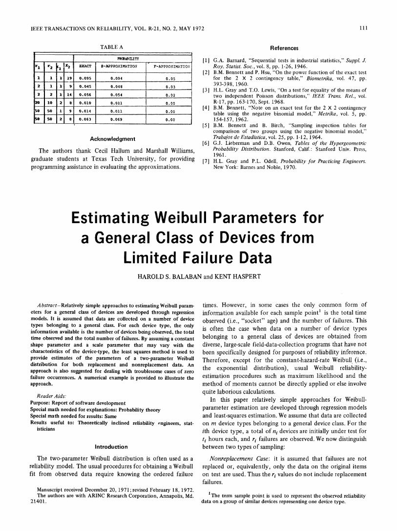
TABLE A References
PR(EABMLITY J_ [1] G.A. Barnard, "Sequential tests in industrial statistics," Suppl. J.r1 r2 1 EXACT B-APPROXIMATION F-APPROXIMATION Roy. Statist. Soc., vol. 8, pp. 1-26, 1946.
[21 B.M. Bennett and P. Hsu, "On the power function of the exact test1 1 1 19 0.095 0.094 0.05 for the 2 X 2 contingency table," Biometrika, vol. 47, pp.2 1 1 9 0.045 0.048 0.03 393-398, 1960.
[3] H.L. Gray and T.O. Lewis, "On a test for equality of the means of2 2 1 14 0.056 0.054 0.02 two independent Poisson distributions," IEEE Trans. Rel., vol.
20 10 2 8 0.010 0.011 0.00 R-17, pp. 163-170, Sept. 1968.0 50 1L 9 0.01.4 0.011 0.00 [4] B.M. Bennett, "Note on an exact test for the 2 X 2 contingency50 50
__t9 0.010.011 0.00table using the negative binomial model," Metrika, vol. 5, pp.
so50 2 8 0.063 0.069 0.00 154-157, 1962.
[5] B.M. Bennett and B. Birch, "Sampling inspection tables forcomparison of two groups using the negative binomial model,"
Acknowledgment Trabajos de Estadistica, vol. 25, pp. 1-12, 1964.[6] G.J. Lieberman and D.B. Owen, Tables of the Hypergeometric
The authors thank Cecil Hallum and Marshall Williams, Probability Distribution. Stanford, Calif.: Stanford Univ. Press,graduate students at Texas Tech University, for pro g [7] H.L. Gray and P.L. Odell, Probability for Practicing Engineers.programming assistance in evaluating the approximations. New York: Barnes and Noble, 1970.
Estimating Weibull Parameters fora General Class of Devices from
Limited Failure DataHAROLD S. BALABAN and KENT HASPERT
Abstract-Relatively simple approaches to estimating Weibull param- times. However, in some cases the only common form ofeters for a general class of devices are developed through regression information available for each sample point' is the total timemodels. It is assumed that data are collected on a number of device observed (i.e., "socket" age) and the number of failures. Thistypes belonging to a general class. For each device type, the only is often the case when data on a number of device typesinformation available is the number of devices being observed, the total often to a gen dass of devic e from
time observed and the total number of failures. By assuming a constant belonging to a general class of devices are obtained fromshape parameter and a scale parameter that may vary with the diverse, large-scale field-data-collection programs that have notcharacteristics of the device-type, the least squares method is used to been specifically designed for purposes of reliability inference.provide estimates of the parameters of a two-parameter Weibull Therefore, except for the constant-hazard-rate Weibutl (i.e.,distribution for both replacement and nonreplacement data. Anapproach is also suggested for dealing with troublesome cases of zero Xe
failure occurrences. A numerical example is provided to illustrate the estimation procedures such as maximum likelihood and theapproach. method of moments cannot be directly applied or else involve
Reader Aids:quite laborious calculations.
Purpose: Report of software development In this paper relatively simple approaches for Weibull-Special math needed for explanations: Probability theory parameter estimation are developed through regression modelsSpecial math needed for results: Same and least-squares estimation. We assume that data are collectedResults useful to: Theoretically inclined reliability engineers, stat- on m device types belonging to a general device class. For the
isticians ith device type, a total of ni devices are initially under test forti hours each, and r1 failures are observed. We now distinguish
Introduction between two types of sampling:
The two-parameter Weibull distribution is often used as a Nonreplacemeni Case: it is assumed that failures are notreliability model. The usual procedures for obtaining a Weibull replaced or, equivalently, only the data on the original itemsfit from observed data require knowing the ordered failure on test are used. Thus the r1 values do not include replacement
failures.Manuscript received December 20, 1971; revised February 18, 1972.The authors are with ARlNC Research Corporation, Annapolis, Md. The term sample point is used to represent the observed reliability
21401. data on a group of similar devices representing one device type.
112 IEEE TRANSACTIONS ON RELIABILITY, MAY 1972
Replacement Case: it is assumed that a replacement is The mean life of an item is a' /Ir(I/0+± 1).inmediately made upon device failure, and failures of replace- f is known as the shape parameter, and ax is known as thements are included in the observed ri values. scale parameter. We assume that the shape parameter of the
We also include the possibility that for each device type generic device class is constant, i.e., ( is independent of thethere may be an associated vector of parameters Pi, which may parameter vector P. However, we assume that the scalerepresent such factors as application, specific device char- parameter may be functionally related to P, i.e., a is related toacteristics, and reliability-control procedures associated with the attributes of the individual device types within the class.device manufacture, acceptance, or operation. This assumption is reasonable if the underlying form of the
The data for each of the m device types can therefore be time-varying relationship of hazard rate is not influenced byrepresented as a vector Dt = (ei, ty, re, Pc).2 We seek a the Pi vectors but the scaling is. For example, it is commonprocedure to use the limited failure information in the Di's to practice to assume for the exponential case (z = 1) thatobtain a Weibull fit which, in general, will account for the changing P affects the value of the constant hazard rate butdifferences among the device types represented by the not the constancy characteristic.variation in the Pi. From the above assumption, we therefore have the basic
The data situation described above occurs in many relia- modelbility research studies, especially those that have the overall / topurpose of developing a reliability model or prediction R(t; P) = exp a- (4)procedure for a general class of items. As an example, in a )recently completed study on monolithic integrated circuits where o(P) is used to show the dependence of the scale[1], data on 111 device types in 17 systems were obtained parameter on the device-parameter vector P. The applicationfrom various industry and government sources. Detailed data of (4) will be considered separately for nonreplacement andon device screening, burn-in, construction, and application replacement data.were available. However, the existing data-collection programscould provide failure-time information only at the system Analysis of Nonreplacement Datalevel-if at all-because it was not practical in many of theprograms to maintain records at the device level. Therefore, at If ri failures are observed when ni items are each tested forthe device level, the only failure information available was ti hours without replacement, a commonly used non-total operating time and number of failures for each of the parametric estimate of reliability for the ith device type overdevice types. (0, ti) can take either of two forms:A somewhat similar data restriction is considered in
reference [2] for obtaining maximum-likelihood estimates ni- ri(a)when the exponential distribution is assumed. Failure times niare not known, but the number of failures occurring within R(ti)
n
specified test-time intervals is known. All test items are lni+ 1 - l (Sb)assumed to have the same exponential distribution, which is a \ ± 1much simpler reliability model than that considered here.
Equation 5a is appropriate when the time of observation (t,) isThe Webl.itiuina eibl o
fixed, and Sb is appropriate when the number of failures (ri) ispredetermined [3]. Generally (5a) would be applicable for
The Weibull pdf in the general two-parameter form can be data obtained in field trials. From (4) we haveexpressed as folloWS 3 ln [-lnR(t)] = -Ina(P)+,Blnt. (6)
At) = t exp -t
t, cx, (3>0 (1) We now assume that -In a (P) can be expressed in the linearform
where t represents the time-to-failure. The reliability functionis h
t( (2 -In a (P) = ao + ajg1(P) (7)R(t)=exp\- (2) P I
and the haza,qrd rate fuinc-tion is where ao, a1,, a*are constants to be estimated from the1(t) _ ( data and g1(P) is a known function of P.
z(t) - t~-1. (3) Thus we can use k(t,) as the dependent variable in a linearR(t)a ~~~~~~regression model of the form:
2An example of the type of data considered is presented in Table 4. / i
3B the transformation r = t d(l' /O~the pdf becomes ln [-nI)'a 1 P)bn± 8
pdf{(T '= -a / exp [-(TIa) J. where e is the residual error. We canl apply the least squaresThis form is often used for mathematical convenience. poeueto poiethe estimates A0 Al A A,§2 h
BALABAN AND HASPERT: ESTIMATING WEIBULL PARAMETERS 113
corresponding Weibull parameter estimates are as follows: estimate.A biased estimation procedure to account for the non-
At = ep f-['0 + Aj l lorthogonality due to high intercorrelations has been recentlyU=exp{-[oXj (9) proposed [5]. This technique, called ridge regression, often
1J has the effect of producing the "right" signs. Since the modelA AIAf3=b. (10) proposed here requires that b be positive, if high inter-
correlations exist among the independent variables and ii isTo attain the desirable properties of least squares estimates, negative,introuc ng the ias eacoroft rideges s
i.e., unbiasedness and minimum variance in the set of all linear pedre, itrodcrretfo siga factorytthanaestimators, it is required that the ei have zero mean, a constant c ed lre s ap Te ri ssio npvaiacan'htte enorltd
constrained least-squares approach. The ridge-regression pro-vaSiance andthevatianceofthey e incorrelated. randomvaricedure can also be used to reduce the mean square error overSince the variance of the binomial random v ariable (n- odarllessqrsathexpnefgetrbi.
r)/n approaches zero with increasing n, it can be shown byemploying a general method outlined in [8] that ln [-ln R] isasymptotically unbiased with variance (1 - R)/ [nR(ln R)2] Analysis of Replacement Datafor large n. Therefore, if the model is correct and the sample For replacement data, replacements are made immediatelysizes, ni, are large, the estimates of the regression coefficients' ' '.4 upon device failure. Let fj represent the observed averageare reasonably unbiased.4 number of failures per device application for the ith device
Furthermore, if deemed appropriate or necessary, a min- type i eimum variance condition can be approached under theassumption that the errors are uncorrelated, for then it is fi r=/n. (11)possible to stabilize the variance through a weighted least Thus f1/ti is the observed average failure rate of the ith devicesquares procedure. Using the observed reliability values in thelarge sample variance formula, the sum of squares to be t or th operatinghours.miimze is. For the replacement situation we are considering, f1 ismiinimized iS eqijivalent to an estimate of the mean number of renewals of
m [ h an item that operates t1 hours. The renewal function for aWi Yi- ajXji- bti Weibull distribution is quite complicated and cannot be
i= L j=0 L obtained in closed form. However, if H(t) is used to representwhere the mean renewal function for any distribution, it can be
shown that the following inequalities hold [61:wi-niR(ti)[ln (ti)]
IR1()1-(t) S H(t) < [ I1-R(t)I IR(t). (12)Yi-n [-in k(t1)J
We now consider the relationship between -In R(t) andXji the jth independent variable for the ith observation (Xoi H(t). By the Maclaurin expansion for the natural logarithm,
= 1). it can be shown that-In x > 1-x for 0< x < I so that
The above procedure is analogous to the commonly used -In R(t)> 1 - R(t). To prove that -n R(t) . [1 -R(t)] /R(t)graphical procedure for a Weibul fit with grouped data (e.g., we can consider the equivalent inequality R(t)[1 -lnR(t)] < 1.
see Reference [4] ) except that least-squares theory is used to Since the derivative of x(1 - In x) is positive over (0, 1] andpredict the shape and scale parameters for a given set of device negative thereafter, the maximum value of R(t) [I - In R(t)]characteristics under the assumption that : is constant over the is 1, which occurs when R(t) = 1. Therefore, analogous todevice class. (12), we have
Since we must have ,B > 0 for a valid pdf, some form of a 1 - R(t) < -In R(t) < [1 - R(t)] /R(t). (13)constrained least-squares procedure may have to be used tosatisfy the implied constraint of i > 0. However, it is If R represents the true reliability of a device, thecautioned that a negative b based on ordinary least squares maximum absolute error of the approximationd-ln R(t)may indicate that the Weibull assumption or the regression H(t) is represented by the range of the H(t) bounds; thusmodel is inappropriate.
If there is high correlation among the predictor variables, t, Emax = max H + inRIg1 (P), g2 (P), * * *, gh (P), the correlation matrix representing - l R R 1 R - R /these variables will be far from an identity matrix and the =-(1 -R)/ -(1 -R)=(-R(-)2/R.regression problem is said to be ill-conditioned. Such a If R = 0.80, the maximum error is 0.050. It decreases tosituation may also lead to an implausible sign for a regression 0.0111 forR-=0.90 and to 0.00.0101 forR = 0.99.coefficient because of the large uncertainty in the least squares A further error analysis was made by the use of computer
simulation. For ct fixed at 10 and ,B = 1/3, 2/3, 2, and 3, a4For two different simulation runs which are described in a later total of 10,000 simulations of Weibull times was obtained for
section, the bias appears to be well within tolerable limits. By using assumed R values of 0.8, 0.9, and 0.95. The observed meanTaylor's expansions to the second order term, the bias in'ln [-ln(1-r/n)l can be shown to be approximately R(l1-R)/2n which numbers of renewals per device were compared with -ln R.is quite small if reliability is close to 1.0 or nis large. The results, which are presented in Table 1, show the
114 IEEE TRANSACTIONS ON RELIABILITY, MAY 1972
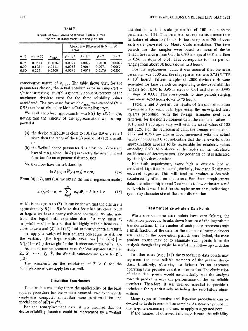
TABLE 1 distribution with a scale parameter of 100 and a shapeResults of Simulations of Weibuil Failure Times parameter of 1.25. This parameter set represents a mean time
for a = 10.0 and Various R and ,B Values to failure of about 37 hours. Fifteen samples of 200 devices
Absolute = lObserved H(t) + In RI each were generated by Monte Carlo simulation. The timeError periods for the samples were based on assumed device
R(t) -In R(t) elx 1|= 1/3 1 = 2/3 a = 2 a = 3 reliabilities ranging from 0.50 to 0.90 in steps of 0.05 and then__max to 0.96 in steps of 0.01. This corresponds to time periods0.95 0.0513 0.00263 0.0029 0.0037 0.0018 0.00039 ranging from about 30 hours down to 3 hours.0.90 0.1054 0.0111 0.0058 0.0054 0.0071 0.0052 rangm utp30choursdownt 3 hours.0.80 0.223J 0.0500 | 0.0246 0.0079 0.0176 0.0203 For the replacement data, itwas assumed that the scale
parameter was 5000 and the shape parameter was 0.75 (MTTF105 hours). Fifteen samples of 2000 devices each were
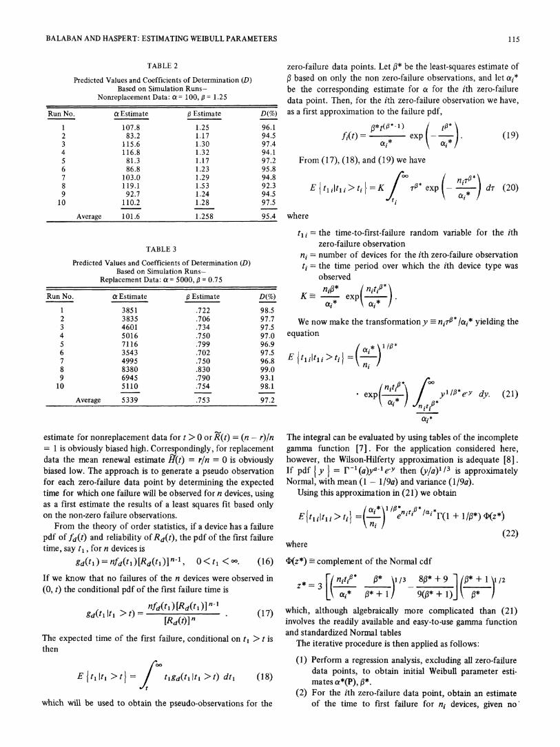
conservative nature of Cmax, The table shows that, for the generated for time periods corresponding to device reliabilitiesparameters chosen, the actual absolute error in using H(t) = ranging from 0.90 to 0.95 in steps of 0.01 and then to 0.995r/n for estimating -In R(t) is generally about 50 percent of the in steps of 0.001. This corresponds to time periods rangingmaximum absolute error for the three reliability values from about 4250 hours down to 75 hours.considered. The two cases for which emax was exceeded (R = Tables 2 and 3 present the results of ten such simulation0.95) can be attributed to Monte Carlo sampling error. experiments for each data type using the unweighted leastWe shall therefore approximate -lnR(t) by H(t) = r/n, squares procedure. With the average estimates used as a
noting that the validity of the approximation will be sup- criterion, for the nonreplacement data, the estimated values ofported if 101.6 and 1.258 agree very well with the actual values of 100
and 1.25. For the replacement data, the average estimates of(a) the device reliability is close to 1.0, (say 0.9 or greater) 5339 and 0.753 are also in good agreement with the actual
since then the range of the H(t) bounds of(12) is small; values of 5000 and 0.75, indicating that the renewal-functionor approximation appears to be reasonable for reliability values
(b) the Weibull shape parameter, is close to 1 (constant exceeding 0.90. Also shown in the tables are the calculatedhazard rate), since -In R(t) is exactly the mean renewal coefficients of determination. The goodness of fit is indicatedfunction for an exponential distribution. by the high values obtained.
We therefore have the relationships For both experiments, every high a estimate had anassociated high ,3 estimate and, similarly, low a and j3 estimates-In R(ti) ;H(ti) = i = r/ln-. (14) occurred together. This will tend to produce a desirable
From (4), (7), and (14) we obtain the linear regression model: counteracting effect on the errors. For the nonreplacementdata, the ratio of high ot and ,B estimates to low estimates was 6
h to 4, while it was 5 to 5 for the replacement data, indicating aIn (r/n) = aO + E a,g1(P) + b In t + C (15) symmetry characteristic of the error distribution.
j=lI
which is analogous to (8). It can be shown that the bias in e isapproximately R(l - R)/2n so that for reliability close to 1.0 Treatment of Zero-Failure Data Pointsor large n we have a nearly unbiased condition. We also note When one -or more data points have zero failures, thefrom the logarithmic expansion that, for very small x, estimation procedure breaks down because of the logarithmicIn [-ln(1 - x)] In x so that for highiy reliable items r/n is transformations. If the number of such points represents onlyclose to zero and (8) and (15) lead to nearly identical results. a small fraction of the data, or the number of sample devices
To apply a weighted least squares procedure to stabilize was small, or the observation periods were limited, the mostthe variance (for large sample sizes, var j ln (r/n) } - prudent course may be to eliminate such points from theRI [n(l- R)] ) the weight for the ith observation is niril(ni- re). analysis though they might be useful in a follow-up validation
As in the nonreplacement case, for least-squares estimates study.A A A A,a0, al, * * *, ah, b, the Weibull estimates are given by (9), In other cases (e.g., [1]) the zero-failure data points may(10). represent the most reliable members of the generic device
The comments on the restriction of b > 0 for the class. Intuitively, observing no failures for an extendednonreplacement case apply here as well. operating time provides valuable information. The elimination
of these data points would automatically bias the analysistowards predicting only the performance of the less reliable
Simulation Experimentsmembers. Therefore, it was deemed essential to provide aTo provide some insight into the applicability of the least technique for quantitatively including the zero failure obser-
squares procedure for the models assumed, two experiments vations.employing computer simulation were performed for the Many types of iterative and Bayesian procedures can bespecial case of a(P) = e0O, devised to include zero-failure samples. An iterative procedure
For the nonreplacement data, it was assumed that the that is quite elementary and easy to apply is suggested here.device-reliability function could be represented by a Weibull If the number of observed failures, r, is zero, the reliability
BALABAN AND HASPERT: ESTIMATING WEIBULL PARAMETERS 115
TABLE 2 zero-failure data points. Let ,B* be the least-squares estimate of
Predicted Values and Coefficients of Determination (D) f based on only the non zero-failure observations, and let ai*Based on Simulation Runs- be the corresponding estimate for a for the ith zero-failure
Nonreplacement Data: a =100, = 1.25 data point. Then, for the ith zero-failure observation we have,Run No. ca Estimate , Estimate D(%) as a first approximation to the failure pdf,
2 4601 .734 97.7 We now make the transformationy -ni7r9 /ai* yielding the4 5016 .750 97.0 equation5 7116 .799 96.9 1/1*6 3543 .702 97.5 E7 4995 .750 96.8 tjtj> 18 8380 .830 99.0 n9 6945 .790 93.110 5110 .754 98.1 niti\ / y
Average 5339 .753 97.2 ta1 *1I)J *nii
estimate for nonreplacement data for t > 0 or R(t) = (n - r)/n The integral can be evaluated by using tables of the incomplete= 1 is obviously biased high. Correspondingly, for replacement gamma function [7]. For the application considered here,data the mean renewal estimate H(t) = r/n = 0 is obviously however, the Wilson-Hilferty approximation is adequate [8].biased low. The approach is to generate a pseudo observation If pdf {y = P1 (a)yal1e-Y then (y/a)1/3 is approximatelyfor each zero-failure data point by determining the expected Normal, with mean (1 - 1/9a) and variance (1/9a).time for which one failure will be observed for n devices, using Using this approximation in (21) we obtainas a first estirmate the results of a least squares fit based only
ai * I /# *on the non-zero failure observations. E{tijjt1j>tj} = ni e r(i + 1/g*) (I(z*)
From the theory of order statistics, if a device has a failure \22)pdf of fd(t) and reliability of Rd(t), the pdf of the first failure (22)time, say t1, for n devices is
gd(tl) = nfd(tl)[Rd(tl 0< t1 <00. (16) 1{z*) complement of the Normal cdf
If we know that no failures of the n devices were observed in F3 niti3 ,B* \1/3 813* + 91 /* + 1_\/2(0, t) the conditional pdf of the first failure time is Z3L * (*+ 1) 9(*±+ I)J1 (* /
gd(tl It1 >t) = nfd(tl)IRd(tl)] (17) which, although algebraically more complicated than (21)[Rd(t)] n~ involves the readily available and easy-to-use gamma function
and standardized Normal tablesThe expected time of the first failure, conditional on t1 > t is Thitrivpocdeishnapldasflw:
thenTh trtvprcdr1Ste pleasflo:z ~~~~~~~~~(1)Perform a regression analysis, excluding all zero-failure
E itlltl ti=j tlg(tlItl >t dt, (18)data points, to obtain initial Weibull parameter esti-
t (2) For the ith zero-failure data point, obtain an estimatewhich will be used to obtain the pseudo-observations for the of the time to first failure for n1 devices, given no
116 IEEE TRANSACTIONS ON RELIABILITY, MAY 1972
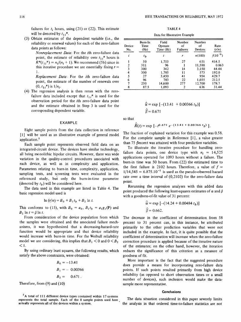
failures for ti hours, using (21) or (22). This estimate TABLE 4will be denoted by t, jt. Data for Illustrative Example
(3) Obtain estimates of the dependent variable (i.e., the *-reliability or renewal values) for each of the zero-failure Bum-In Field Number Number
Device Time Operate of of Ratedata points as follows: No. (Hr) Time (Hr) Failures Devices (rln)
Nonreplacement Data: For the ith zero-failure data tb r n(100) f(10 -6)point, the estimate of reliability over t j* hours isR*(tli*)= nil(ni + 1). We recommend (5b) since in 1 50 1,753 27 651 414.5this iterative procedure we are essentially fixingr= 2 311 96 1 11,588 0.8633 300 342 14 3,150 44.441. 4 300 1,785 1 1 573 192.0Replacement Data: For the ith zero-failure data 5 27 3,450 41 954 429.7point, the estimate of the number of renewals over 6 96 783 22 1,035 212.5
ol ti M isIIni. ~~~~7 250 14,600 277 12,700 178.7(0, t11*) is 1/n1. 8 87.5 1,093 2 636 31.44
(4) The regression analysis is then rerun with the zero-failure data included except that t1 * is used for theobservation period for the ith zero-failure data point Aand the estimate obtained in Step 3 is used for the a =exp [-(13.41 ± 000366 tb)Icorresponding dependent variable. A=0.671
so thatEXAMPLE =exp [_t0671 e-(1 3.41 + 0.00366 tb) ]
Eight sample points from the data collection in reference[1] will be used as an illustrative example of general model The fraction of explamed vaiation for this example was 0.58application.5 For the complete sample in Reference [1], a value greater
Each sample point represents observed field data on an than 75ipercenthwas attainedwithfourpredictiondvariablesintegrated-circuit device. The devices have similar technology, To illustrate the iterative procedure for handling zero-all being monolithic bipolar circuits. However, there was wide failure data poits, one device type with n1 = 14,525variation in the quality-control procedures associated with applications operated for 1093 hours without a failure. Theeach device, as well as in complexity and application. burn-in time was 50 hours. From (22) the estimated time toParameters relating to burn-in time, complexity, application, the first failure is 2102 hours. Therefore, a value of f =
sampling tests, and screening tests were evaluated in the I1/14,545 = 6.875.10 is used as the pseudo-observed hazard
referenced study, but only the burn-in-time parameter rate over a time interval of (0,2102) for the zero-failure data
(denoted by tb) will be considered here. point.The data used in this example are listed in Table 4. The Rerunning the regression analyses with this added data
basic regression model used is point produced the following least-squares estimates of a and 13with a goodness-of-fit value of 31 percent:
In (r/n) = Bo + Bl tb + B2 ln t. Aa = exp [-(14.24 ± 0.00484 tbI
This conforms to (15), with Bo = ao, Bitb = alg1(P) and AB2 ln t =1,ln t. 1 = 0.662.
From consideration of the device population from which The decrease in the coefficient of determination from 58the samples were obtained and the associated failure mech- percent to 31 percent can, in this instance, be attributedanisms, it was hypothesized that a decreasing-hazard-rate primarily to the other prediction variables that were notfunction would be appropriate and that device reliability included in the example. In fact, it is quite possible that thewould increase with burn-in time. For the Weibull reliability coefficient of determination will increase when the zero-failuremodel we are considering, this implies that BI < 0 and 0 < B2 correction procedure is applied because of the iterative nature< 1. of the estimates; on the other hand, however, the iteration
By using ordinary least squares, the following results, which reduces the significance of this criterion as a measure ofsatisfy the above constraints, were obtained: goodness of fit.
Bn= -13.41 AMore important is the fact that the suggested procedureB0 =-13.41 ~~~does provide a means for incorporating zero-failure data
B1 =-0.00366 points. If such points resulted primarily from high device
B2 = 0.671. ~~~~reliability (as opposed to short observation times or a smallB2 = 0.671. ~~~number of devices), such inclusion would make the data-
Therefore, from (9) and (10) sample more representative.
Conclusions5A total of 111 different device types contained within 17 systems
represents the total sample. Each of the 8 sample points used here~ The data situation considered in this paper severely limitsactually represents all of the devices within a system. the analysis in that ordered time-to-failure statistics are not
IEEE TRANSACITIONS ON RELIABILITY, MAY 1972 117
available. The basic reliability characteristic assumed-a time- Referencesvarying hazard-rate function as represented by a Weibull [1] J. Reese, "Reliability prediction for monolithic integrated cir-probability distribution-and possibly Weibull parameter var- cuits," ARINC Research Corp., Publ. 947-01-1-1143, Nov. 1971.iation as a function of device design, manufacture, and control [2] P.J. Kendall and R.L. Anderson, "An estimation problem in lifetesting," Technometrics, vol. 13, pp. 289-301, May 1971.procedures, compounds the severity of the problem. [3] G.R. Herd, "Estimation of reliability from incomplete data," in
This situation, however, is not at all uncommon, especially Proc. 6th Nat. Symp. Rel. Quality Contr., Jan. 1960, pp. 190-201.when diverse general-purpose data-collection programs are the [41 W. Nelson, "Hazard plotting for incomplete failure data," J.Quality Technol., vol. 1, pp. 27-52, Jan. 1969.main data source. The model described in this paper is believed [5] A.E. Hoerl and R.W. Kennard, "Ridge regression: Biased esti-to represent a reasonable and practical approach overcoming mation for nonorthogonal problems," Technometrics, vol. 12, pp.the limitations inherent in. the available data. However, further 55-67, Feb. 1970.[6l B.V. Gnedenko, Yu. K. Belyayev, and A.D. Solovyev, Math-study of the statistical properties of the estimates is necessary ematical Methods of Reliability Theory. New York: Academic,for the measurement and control of bias and the development 1969, pp. 96-102.of procedures for variance analysis and confidence-interval [7] K. Pearson, Tables of the Incomplete Gamnm Function. London:
Cambridge Univ. Press, 1934.prediction. [8] M.G. Kendall and A. Stuart, The Advanced Theory of Statistics,
vol. 1, 3rd ed. Hafner: 1969, pp. 231-232, 371-374.
Notesi
A System Reliability with Pay-Offs operable state to the failed state and vice versa, it incurs certain loss,which has been assumed to be instantaneous. This loss does not increasewith time as long as the system stays in the same state. A numerical
N. SINGH and SANTOSH KUMAR example illustrates the procedure.
Abstract-A mathematical model incorporatig pay-offs in a reliabilitycontext has been developed. This idea is of interest when systems are Notationshighly reliable but the risk involved with the associated unreliability is The following notation is used in formulating the model:equally great. A numerical example illustrates the procedure.
A Poisson parameter representing the failure rate of theReader Aids: component.
Purpose: Report of software derivation j Poisson parameter representing the repair rate of the failedSpecial math needed for explanations: Matrix notation, probability component.theory A The differential coefficients transition matrix whose ele-Special math needed for results: Same ments depend on X and ,.Results useful to: Reliability engineers L Loss matrix
a# transition rate of the system from state i to state j; (i # j).Vi(t) expected total loss in time t, when the system is in state i at
Introduction the end of time t.
Various measures of dependability have been defined suiting certain lj instantaneous loss when the system makes a transition fromsituations. Hosford [ 11 has pointed out that among the existing state i to state j (i t j).measures, pointwise availability, reliability and interval availability are sum from I to N, except as noted.important measures to give the correct estimate of the system understudy. However, in situations where risk is involved, these measures arenot appropriate. For example, a power plant, blast furnace, or any Mathematical Formulation of the Problemindustrial system needing corrective maintenance if it fails can result ina disaster both in terms of security and money. In such situations, it is With the help of conditional probability considerations, the ex-worthwhile to devise some measures to weigh the risk which may be in pected total loss in time t + A can be related to the expected loss interms of units of money-pay-offs. For such cases it is, therefore, desired time t as follows (multiple transitions in a small interval of timne A arethat systems reliability with pay-offs be studied. Keeping this in view, not allowed):in this note, a mathematical model incorporating pay-offs in reliabltyhas been developed. When the system makes a transition ftom the V,(t+ A)=(1-j ai.iA)V1(t)
Manuscript received March 8, 1971; revised Septemberl10,1971. ]S.Kmri ihteRylMelbourne, Intiut of00 Technology,
Define the diagonal elements of the matrix A byN. Singh is with the Department of Mathematics, Monash University, a g =- z a.. (2)Clayton, Vic. 3168, Australia. frie V