ESTIMATION AND EXTRAPOLATION OF TIME TRENDS INREGISTRY DATA—BORROWING STRENGTH FROM
RELATED POPULATIONS
BY ANDREA RIEBLER1,2, LEONHARD HELD1 AND HÅVARD RUE
University of Zurich, University of Zurich and Norwegian Universityof Science and Technology
To analyze and project age-specific mortality or morbidity rates age-period-cohort (APC) models are very popular. Bayesian approaches facil-itate estimation and improve predictions by assigning smoothing priors toage, period and cohort effects. Adjustments for overdispersion are straight-forward using additional random effects. When rates are further stratified, forexample, by countries, multivariate APC models can be used, where differ-ences of stratum-specific effects are interpretable as log relative risks. Here,we incorporate correlated stratum-specific smoothing priors and correlatedoverdispersion parameters into the multivariate APC model, and use Markovchain Monte Carlo and integrated nested Laplace approximations for infer-ence. Compared to a model without correlation, the new approach may lead tomore precise relative risk estimates, as shown in an application to chronic ob-structive pulmonary disease mortality in three regions of England and Wales.Furthermore, the imputation of missing data for one particular stratum maybe improved, since the new approach takes advantage of the remaining strataif the corresponding observations are available there. This is shown in an ap-plication to female mortality in Denmark, Sweden and Norway from the 20thcentury, where we treat for each country in turn either the first or second halfof the observations as missing and then impute the omitted data. The pro-jections are compared to those obtained from a univariate APC model andan extended Lee–Carter demographic forecasting approach using the properDawid–Sebastiani scoring rule.
1. Introduction. Most developed countries have national health registers toroutinely collect demographic rates. Age-period-cohort (APC) models are com-monly used to analyze and project mortality or morbidity rates, in which effectsrelated to the age of an individual, calendar time (period) and the generation (co-hort) can reasonably be assumed to be present. When several of such register datasets are available, for example, for different countries, each data set could be ana-lyzed separately by a univariate APC model. However, for comparable strata, sim-ilar unobservable factors are likely to act on the different time dimensions (age,
Received July 2010; revised May 2011.1Supported by the Swiss National Science Foundation.2Supported by the Research Council of Norway.Key words and phrases. Bayesian analysis, INLA, multivariate age-period-cohort model, projec-
period, cohort), so that a multivariate APC analysis may seem more appropriate[Hansell et al. (2003), Hansell (2004), Jacobsen et al. (2004), Riebler and Held(2010)].
A quirk of APC models is the obvious linear dependence of age, period and co-hort effects leading to a well-known identifiability problem. Over the last decadesseveral proposals, ranging from the specification of additional identifying restric-tions to the definition of estimable functions, have been made to solve the identifi-ability problem; see, for example, Fienberg and Mason (1979), Osmond and Gard-ner (1982), Holford (1983), Robertson and Boyle (1986), Clayton and Schifflers(1987), Holford (1992), Fu (2000), Yang, Fu and Land (2004) or Kuang, Nielsenand Nielsen (2008). Provided that at least one set of age, period or cohort ef-fects is forced to be identical across strata (which is often a plausible assumption),differences of stratum-specific effects in the multivariate APC model are identifi-able without further identifying restrictions. They can be interpreted as log relativerisks, so that heterogeneous time trends, for example, across gender [Riebler et al.(2011)] or geographical regions [Hansell (2004), Riebler and Held (2010)], can beanalyzed.
Bayesian APC analyses have become very popular in the last years; see, for ex-ample, Nakamura (1986), Berzuini and Clayton (1994), Besag et al. (1995), Ogataet al. (2000), Knorr-Held and Rainer (2001), Bray, Brennan and Boffetta (2001),Bray (2002), Baker and Bray (2005), Schmid and Held (2007), Riebler and Held(2010). As effects adjacent in time are likely to be similar, smoothing priors aretypically assumed for age, period and cohort effects. Nakamura (1986) used first-order autoregressive priors, while Berzuini and Clayton (1994) and Besag et al.(1995) proposed to use second-order random walks. The second-order randomwalk is a discrete-time analogue of a cubic smoothing spline [Fahrmeir and Tutz(2001)]. This prior is defined on the identifiable second differences, a well-knownmeasure of curvature, and penalizes deviations from a linear trend [Fienberg andMason (1979), Clayton and Schifflers (1987)]. The degree of smoothness is con-trolled by an unknown smoothing parameter. Using smoothing priors, overfittingcohorts, which by design are sparsely represented, is avoided [Besag et al. (1995)].
When age group and period intervals are of different length, an additional identi-fiability problem may induce artificial cyclical patterns in the parameter estimatesof uni- and multivariate APC models; see Holford (2006) and Riebler and Held(2010), respectively. However, this problem can be solved by applying smooth-ing functions, such as second-order random walks or penalized splines [Holford(2006)]. The assumed smoothness of age, period and cohort effects can also beexploited for providing projections, as the effects can easily be extrapolated intoboth the future and past [Knorr-Held and Rainer (2001), Bray (2002)]. In a hi-erarchical Bayesian model, additional random effects can be included to accountfor heterogeneity without temporal structure [Berzuini and Clayton (1994), Besaget al. (1995)].
306 A. RIEBLER, L. HELD AND H. RUE
Riebler and Held (2010) assumed independent smoothing priors for stratum-specific effects in multivariate APC models. Here, we propose to link stratum-specific smoothing priors. The new approach leads to a multivariate correlatedrandom walk, where the joint precision matrix is defined as the Kronecker productof the inverse of a uniform correlation matrix and the precision matrix of the uni-variate second random walk. Inference is done using Markov chain Monte Carlo(MCMC) and integrated nested Laplace approximations [Rue, Martino and Chopin(2009)].
The new specification can be regarded as shrinking the stratum-specific param-eters toward some common trend. Indeed, an alternative model formulation wouldintroduce a common period effect, say, modeled via a second order random walkand additionally independent second order random walks for each stratum. Whilethis formulation has two variance parameters, it in fact induces correlation betweenthe stratum-specific increments, which are defined as the sum of the common in-novation and the stratum-specific innovations, so that it can be translated into amultivariate random walk with one variance and one correlation parameter.
In time series analysis, the use of multivariate random walks plays a fundamen-tal role in multivariate modeling [Harvey (1990)]. The multivariate random walkis an example of an intrinsic multivariate Gaussian Markov random field (GMRF)model [Rue and Held (2005)]. Multivariate GMRF models with conditional autore-gressive (CAR) structure are sometimes called multivariate CAR (MCAR) models;see, for example, Gelfand and Vounatsou (2003) or Carlin and Banerjee (2003).Proper multivariate GMRF models have been introduced by Mardia (1988). Grecoand Trivisano (2009) applied MCAR models to handle general forms of spatial de-pendence occurring in multivariate spatial modeling of area data. Lagazio, Biggeriand Dreassi (2003) and Schmid and Held (2004) used Kronecker product precisionmatrices to model different types of space–time interactions in spatial APC models[Knorr-Held (2000)]. However, as far as we know, correlated second order randomwalks have never been used in multivariate APC models.
We further propose the incorporation of correlated overdispersion parametersto model unobserved risk factors without temporal structure but acting simultane-ously on the different strata. The use of correlated overdispersion parameters issimilar in spirit to seemingly unrelated regressions, where single regression equa-tions are linked by correlated error terms [Harvey (1990)].
Through the introduction of correlation in the prior distribution the effectivedegrees of freedom are reduced whenever similar behavior in the different strataexists. Hence, the precision of relative risks may be improved. Furthermore, theapproach is useful to predict missing records in one particular stratum if the cor-responding data are available for the remaining strata. This might be the case forhistorical data if the collection of demographic rates started not at the same timein different strata. Consider, for example, Switzerland, where each canton (ad-ministrative unit) is separately responsible for the implementation of health-policyinstruments, so that cancer is registered on a cantonal level [Ess et al. (2010),
CORRELATED MULTIVARIATE APC MODELS 307
Bouchardy, Lutz and Kühni (2011)]. The first Swiss cancer registration systemstarted in 1970 in the canton of Geneva followed by registers in the cantons ofVaud and Neuchâtel in 1974 [Bouchardy, Lutz and Kühni (2011)]. Compared toother cantons without explicit cancer registration, extensive cancer analyses havebeen performed for these cantons; see, for example, Levi et al. (1993, 1998, 2002),Verkooijhen et al. (2003). Today most cantons have cancer registers and it isplanned that within the next years the entire Swiss population will be capturedby a cancer registration system [Bouchardy, Lutz and Kühni (2011)]. Our methodcan be used to impute missing data for cantons with a younger cancer registrationsystem taking advantage of other cantons with a longer collection period. Thus,important insight into cancer progression for all cantons could be gained. A differ-ent aspect might be varying collection intervals in different regions, where in someregions data are collected on a yearly basis, say, and in other regions on a five-yearbasis. Here, the correlated multivariate APC approach may be used to impute therates for the missing years. In this paper, we demonstrate the ability to imputemissing data units in a cross-prediction study of female mortality in Scandinavia.
The paper is organized as follows. Section 2 introduces the two applicationspresented in this paper. In Section 3 we review multivariate APC models and in-troduce our extended correlated approach (Section 3.1). Then we present detailson the implementation (Section 3.2). In Section 4 we present the results of the twoapplications. Our findings are summarized in Section 5.
2. Applications.
2.1. Analysis of heterogeneous time trends in COPD mortality among malesin England and Wales. We reanalyze male mortality data on chronic obstructivepulmonary disease (COPD) in three regions of England and Wales: Greater Lon-don, conurbations excluding Greater London and rural areas (nonconurbations).COPD is one of the most common lung diseases making it hard to breathe as aconsequence of limited air flow. One of the main causes of COPD is smoking,but also air pollution, smog, dust and chemical fumes are relevant risk factors.While smoking exerts mainly long-term effects with a lag period of about 20–30years [Kazerouni et al. (2004)], air pollution can cause both long-term (period orcohort) effects and short-term (period) effects [Sunyer (2001), Dockery and Pope(1994)]. We focus on short-term effects and the relation between marked air pol-lution events and changes in COPD mortality. For all regions data are availableon an annual basis from 1950–1999 for seven age groups: 15–24, 25–34, . . . ,75+[Hansell et al. (2003), Hansell (2004)]. Riebler and Held (2010) analyzed hetero-geneous time trends in these data using an uncorrelated multivariate APC modelwith common age effects. We will compare their results with those obtained froma model with correlated stratum-specific period, cohort and overdispersion param-eters.
308 A. RIEBLER, L. HELD AND H. RUE
2.2. Extrapolation of overall mortality of Scandinavian females. All data wereobtained from the Human Mortality Database (2011). The number of deaths arestratified by 5-year groups, for all Norwegian, Danish and Swedish women aged0–84 in the period 1900–1999, leading to 17 age groups (0–4, 5–9, . . . ,80–84)and 20 periods (1900–1904, . . . ,1995–1999). Figure 1 shows the death rates per1,000 person-years for all three countries stratified by 5-year age groups. To ob-tain person-years, we used the yearly population sizes available for the same agegroups and based on the 1st of January. We used linear interpolation to get mid-year estimates and then added up the resulting quantities to obtain person-yearsfor 1900–1904, . . . ,1995–1999. The rates of all three countries show a very sim-ilar progression. The peak in mortality in the 1915–1919 period, present, in par-ticular, among young adults, is supposed to be related to the 1918–1919 Spanishflu pandemic which killed about 50 million people worldwide, with most deathsoccurring among young adults [Andreasen, Viboud and Simonsen (2008)]. Duringthe summer of 1918 there were strong influenza waves in Denmark, Sweden andNorway [Andreasen, Viboud and Simonsen (2008), Kolte et al. (2008)].
FIG. 1. Female death rates per 1,000 person-years (pyrs) in Norway, Denmark and Sweden by agefrom 1900 to 1999. The vertical line divides the time into equally sized parts.
CORRELATED MULTIVARIATE APC MODELS 309
We divide the calendar period into two equally sized parts (see Figure 1). Foreither the first or second half of the 20th century, all observations from one partic-ular country are treated as missing. The omitted data are then predicted exploitingthe information provided by the complete data sets of the other two countries. Thisprocedure is repeated for all countries and hence termed cross-prediction. Thus, wecannot only assess the ability to project particular events present for all countries,such as the Spanish-flu pattern, but also analyze the prediction quality for yearswithout such specific events. The probabilistic projections are compared to thoseobtained from a univariate APC model and to those from an extended Lee–Carterdemographic forecasting model [Lee and Carter (1992)].
The data and code used in this application are provided in the SupplementaryMaterial [Riebler, Held and Rue (2011)].
3. The correlated multivariate APC model. Let yijr denote the number ofdeaths observed for age group i (i = 1, . . . , I ), period j (j = 1, . . . , J ) and stra-tum r (r = 1, . . . ,R). In both of our applications r represents a geographical re-gion (either a region in England and Wales or a Scandinavian country). Deathscan be regarded as events arising from a Poisson process. Hence, yijr can be inter-preted as the number of events that have occurred during an exposure period of nijr
person-years, in which the occurrence rate is assumed to be λijr per person-year.Thus, yijr is Poisson distributed with rate nijrλijr , where nijr is known [Armitage(1966), Brillinger (1986)]. In the most general formulation of the multivariate APCmodel, the linear predictor is
ηijr = log(λijr ) = μr + θir + ϕjr + ψkr .
Here, μr is the stratum-specific intercept, and θir , ϕjr and ψkr are stratum-specificage, period and cohort effects, respectively. The cohort index k is a linear functionof the age index i and the period index j . If the time interval widths of age groupand period are equal, then k = (I − i) + j . If age group intervals are M timeswider than period intervals, as is the case in the first application (Section 2.1)where M = 10, then k = M × (I − i) + j [Heuer (1997)]. We apply the usualconstraints,
∑Ii=1 θir = ∑J
j=1 ϕjr = ∑Kk=1 ψkr = 0 for r = 1, . . . ,R, to ensure
identifiability of the stratum-specific intercepts. However, parameter estimates arestill not identifiable without imposing additional constraints [Fienberg and Mason(1979), Holford (1983)]. In contrast, second differences of parameter estimates, forexample, θir − 2θi−1r + θi−2r , are not affected by the identifiability problem andcan be uniquely determined [Fienberg and Mason (1979), Clayton and Schifflers(1987)]. Furthermore, stratum-specific differences, for example, θir1 − θir2 withr1 �= r2, are identifiable (absent an additional constraint), provided that at least oneof the three time effects (age, period, cohort) is common across strata [Riebler andHeld (2010)].
310 A. RIEBLER, L. HELD AND H. RUE
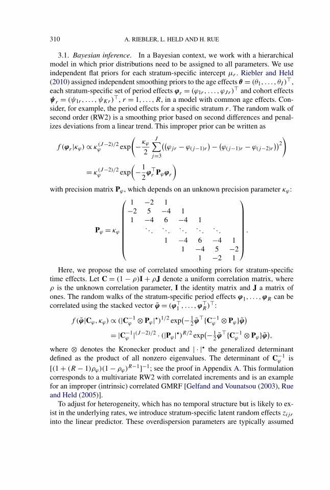
3.1. Bayesian inference. In a Bayesian context, we work with a hierarchicalmodel in which prior distributions need to be assigned to all parameters. We useindependent flat priors for each stratum-specific intercept μr . Riebler and Held(2010) assigned independent smoothing priors to the age effects θ = (θ1, . . . , θI )
�,each stratum-specific set of period effects ϕr = (ϕ1r , . . . , ϕJ r)
� and cohort effectsψ r = (ψ1r , . . . ,ψKr)
�, r = 1, . . . ,R, in a model with common age effects. Con-sider, for example, the period effects for a specific stratum r . The random walk ofsecond order (RW2) is a smoothing prior based on second differences and penal-izes deviations from a linear trend. This improper prior can be written as
f (ϕr |κϕ) ∝ κ(J−2)/2ϕ exp
(−κϕ
2
J∑j=3
((ϕjr − ϕ(j−1)r
) − (ϕ(j−1)r − ϕ(j−2)r
))2)
= κ(J−2)/2ϕ exp
(−1
2ϕ�
r Pϕϕr
)
with precision matrix Pϕ , which depends on an unknown precision parameter κϕ :
Pϕ = κϕ
⎛⎜⎜⎜⎜⎜⎜⎜⎜⎜⎝
1 −2 1−2 5 −4 11 −4 6 −4 1
. . .. . .
. . .. . .
. . .
1 −4 6 −4 11 −4 5 −2
1 −2 1
⎞⎟⎟⎟⎟⎟⎟⎟⎟⎟⎠
.
Here, we propose the use of correlated smoothing priors for stratum-specifictime effects. Let C = (1 − ρ)I + ρJ denote a uniform correlation matrix, whereρ is the unknown correlation parameter, I the identity matrix and J a matrix ofones. The random walks of the stratum-specific period effects ϕ1, . . . ,ϕR can becorrelated using the stacked vector ϕ̃ = (ϕ�
1 , . . . ,ϕ�R)�:
f (ϕ̃|Cϕ, κϕ) ∝ (|C−1ϕ ⊗ Pϕ|)1/2 exp
(−12 ϕ̃�{C−1
ϕ ⊗ Pϕ}ϕ̃)= |C−1
ϕ |(J−2)/2 · (|Pϕ|)R/2 exp(−1
2 ϕ̃�{C−1ϕ ⊗ Pϕ}ϕ̃)
,
where ⊗ denotes the Kronecker product and | · | the generalized determinantdefined as the product of all nonzero eigenvalues. The determinant of C−1
ϕ is[(1 + (R − 1)ρϕ)(1 − ρϕ)R−1]−1; see the proof in Appendix A. This formulationcorresponds to a multivariate RW2 with correlated increments and is an examplefor an improper (intrinsic) correlated GMRF [Gelfand and Vounatsou (2003), Rueand Held (2005)].
To adjust for heterogeneity, which has no temporal structure but is likely to ex-ist in the underlying rates, we introduce stratum-specific latent random effects zijr
into the linear predictor. These overdispersion parameters are typically assumed
CORRELATED MULTIVARIATE APC MODELS 311
to be independent Gaussian variables with mean zero and unknown variance κ−1z ,
that is, zijri.i.d.∼ N (0, κ−1
z ) [Berzuini and Clayton (1994), Besag et al. (1995)].However, when interpreting these latent effects as unobserved covariates, it maybe plausible that they act partly simultaneously on the different strata. Hence, wepropose correlated overdispersion parameters and set zij = (zij1, . . . , zijR)� ∼
N (0, κ−1z Cz) for all i and j .
All of the up to eight hyperparameters (four precisions and up to four corre-lations) are treated as unknown. Suitable gamma-hyperpriors are assigned to theprecisions. As in Knorr-Held and Rainer (2001), we use Ga(1,0.00005) for theprecisions of age, period and cohort effects and Ga(1,0.005) for the precision ofthe overdispersion.
Correlation parameters ρ are reparameterized using the general Fisher’s z-transformation [Fisher (1958), page 219]:
ρ = exp(ρ) − 1
exp(ρ) + R − 1, ρ = log
(1 + ρ · (R − 1)
1 − ρ
),(1)
where ρ can take any real value. It is worth noting that this transformation ensuresthat ρ only takes values within the interval (−1/(R − 1),1), so that C is positivedefinite without imposing an additional constraint. Using R = 2 in (1), we obtain
ρ = exp(ρ) − 1
exp(ρ) + 1, ρ = log
(1 + ρ
1 − ρ
),
which is frequently used for constructing confidence intervals for ρ [Konishi(1985)]. Fisher’s z-transformation is a variance stabilizing transformation. In aBayesian context this transformation is of particular interest since the derivativeof a variance stabilizing transformation corresponds to Jeffreys’ prior for the orig-inal parameter [Lehmann (1999), pages 491 and 492]. For example, for R = 2,Jeffreys’ prior is π(ρ) ∝ 1/(1 − ρ2), the derivative of log(
1+ρ1−ρ
) [Lindley (1965),pages 215–220].
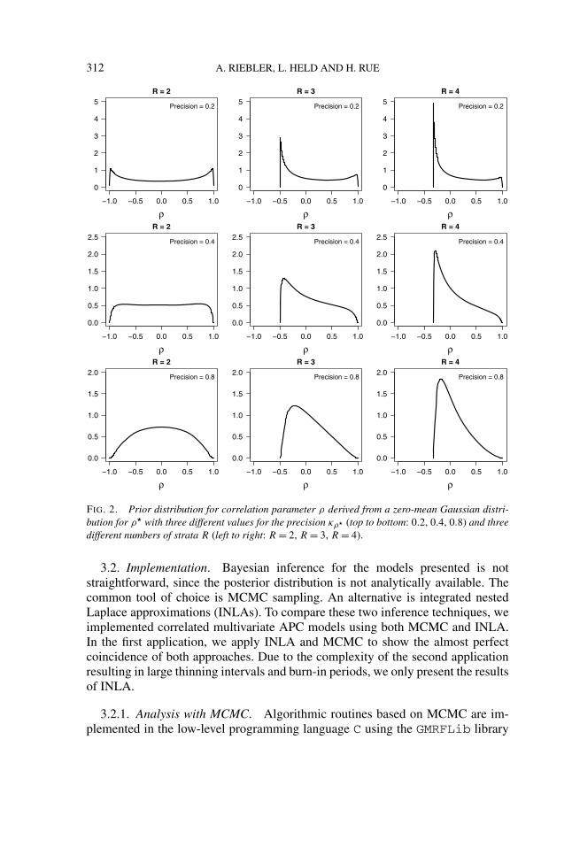
We assign a normal prior with mean zero and fixed precision κρ to ρ. Thus,the prior probability that ρ is larger than zero is equal to 0.5, independent of R.Figure 2 shows the resulting prior for ρ for three different values of κρ and threedifferent values of R. For R = 2 strata, setting κρ to 0.2 corresponds to a U-shapedprior, κρ = 0.4 to a roughly uniform prior and κρ = 0.8 to a bump-shaped priorfor ρ; compare the first column of Figure 2. Note that κρ = 0 corresponds tothe improper Jeffreys’ prior. For a larger number of strata, the left boundary forthe correlation is shifted toward zero, resulting in an asymmetric prior distributionfor ρ, since half of the total density is distributed to a smaller interval, (−1/(R −1),0). We use κρ = 0.2, so that sufficient probability mass is assigned to theboundary values as well, making extreme posterior correlation estimates possible.
312 A. RIEBLER, L. HELD AND H. RUE
FIG. 2. Prior distribution for correlation parameter ρ derived from a zero-mean Gaussian distri-bution for ρ with three different values for the precision κρ (top to bottom: 0.2, 0.4, 0.8) and threedifferent numbers of strata R (left to right: R = 2, R = 3, R = 4).
3.2. Implementation. Bayesian inference for the models presented is notstraightforward, since the posterior distribution is not analytically available. Thecommon tool of choice is MCMC sampling. An alternative is integrated nestedLaplace approximations (INLAs). To compare these two inference techniques, weimplemented correlated multivariate APC models using both MCMC and INLA.In the first application, we apply INLA and MCMC to show the almost perfectcoincidence of both approaches. Due to the complexity of the second applicationresulting in large thinning intervals and burn-in periods, we only present the resultsof INLA.
3.2.1. Analysis with MCMC. Algorithmic routines based on MCMC are im-plemented in the low-level programming language C using the GMRFLib library
CORRELATED MULTIVARIATE APC MODELS 313
[Rue and Held (2005)]. Following Besag et al. (1995), we reparameterize themodel from zijr to ηijr to obtain multivariate normal full conditional distributionsfor the stratum-specific intercepts μ = (μ1, . . . ,μr)
� and all sets of time effects.Block updating allows the proper incorporation of the sum-to-zero constraints forthe time effects. It is also possible to omit the sum-to-zero constraint for one set ofstratum-specific effects and simultaneously remove the stratum-specific interceptsμ from the algorithm. For the precisions Gibbs sampling is used as well. The vectorηij = (ηij1, . . . , ηijR)� has a nonstandard distribution. It is updated using multi-variate Metropolis–Hastings steps with a GMRF proposal distribution based on asecond-order Taylor approximation of the log likelihood [Rue and Held (2005),Section 4.4.1]. For the correlation parameters Metropolis–Hastings updates basedon a random walk proposal are used, such that acceptance rates around 40% areachieved. In the application to COPD mortality we use a MCMC run of 350,000 it-erations, discarding the first 50,000 iterations and storing every 20th sample there-after, resulting in 15,000 samples. We have routinely examined convergence andmixing diagnostics.
3.2.2. Analysis with INLA. Rue, Martino and Chopin (2009) proposed withINLA an alternative deterministic Bayesian inference approach for latent Gaus-sian random field models. INLA replaces time-consuming MCMC sampling withfast and accurate approximations to the posterior marginal distributions. Some em-pirical comparison with MCMC results can be found in Rue, Martino and Chopin(2009), Paul et al. (2010) or Schrödle et al. (2011). We incorporated correlatedGMRF models into INLA, enabling the analysis of correlated multivariate APCmodels based on a uniform correlation structure and using the general Fisher’s z-transformation. The methodology is integrated in the package INLA (see www.r-inla.org) for R [R Development Core Team (2010)]. For both applications, we usethe INLA package built on 14.03.2011.
4. Results.
4.1. COPD mortality among males in England and Wales. We compared theuncorrelated model with joint age-effects, and region-specific period and cohorteffect presented by Riebler and Held (2010) with three different correlated for-mulations: (1) Region-specific period and region-specific cohort effects are corre-lated; (2) the overdispersion parameters are correlated; (3) region-specific periodeffects, region-specific cohort effects and overdispersion parameters are correlated.To make the models comparable, we used, in contrast to Riebler and Held (2010),the same precision for the independent priors of region-specific period effects andalso the same precision for the independent priors of region-specific cohort effects.For all models MCMC and INLA produce virtually identical results; see Figure 3for a comparison of precision and correlation estimates in model 3. The runningtime of INLA was always less than the computation time with MCMC. Inspecting
FIG. 3. Approximated posterior marginal densities (solid red line) of precision and correlation pa-rameters for the multivariate model with joint age effects and correlated period, cohort and overdis-persion parameters obtained from INLA. Moreover, the corresponding histograms of 15,000 MCMCsamples obtained from a run with 50,000 burn-in iterations and a thinning of 20 are shown.
the log marginal likelihood returned by INLA, the model with correlated periodand cohort effects, and correlated overdispersion parameters, was classified as thebest model. Despite the improper random walk prior, the log-marginal likelihoodcan be used here, as the models are based on the same underlying latent struc-ture and only differ by the inclusion of correlation. Furthermore, the correlationestimates ρϕ,ρψ and ρz of model 3 (Figure 3) are clearly different from zero,confirming the between-region dependence.
Figure 4 compares the estimates of average relative risks obtained from MCMCfor the models with uncorrelated and correlated region-specific effects and overdis-persion parameters, respectively. The estimates are relative to nonconurbations,where the mortality rates tend to be the lowest. The results of both models are verysimilar. The average relative risk of period effects shows the typical year-to-yearvariation, with higher values in years of known air pollution events, such as the“Great Smog” in London in 1952. In the average relative risks of cohort effects,different smoking behavior may be visible. For a detailed interpretation of the rel-ative risks we refer to Riebler and Held (2010). Due to fewer observations, thecredible intervals are getting wider for younger birth cohorts. However, adjustingfor correlation improves the precision of the relative risks estimates, in particular,for younger birth cohorts. The average posterior standard deviation in the corre-lated approach is about 20% and 25% smaller for the average relative risks of theperiod effects and cohort effects, respectively.
CORRELATED MULTIVARIATE APC MODELS 315
FIG. 4. Average relative risk of death for Greater London and conurbations excluding GreaterLondon compared with nonconurbations, analyzed by a multivariate model with joint age effects andno correlations across other parameters (top), and a multivariate model with joint age effects andcorrelated period, cohort and overdispersion parameters (bottom). Shown are the median estimateswithin 95% pointwise credible bands.
4.2. Extrapolation of overall mortality of Scandinavian females. We will firstbriefly introduce the basic and the extended Lee–Carter model considered. Thenwe will present the results of the predictive model assessment and compare theprojections obtained by the different approaches.
4.2.1. The quasi-Poisson version of the Lee–Carter model. The Lee–Cartermodel, introduced by Lee and Carter (1992) to forecast mortality in the U.S., is oneof the best-known methods for mortality forecasting and often used as a reference[Booth (2006), Booth et al. (2006)]. It assumes a log-bilinear form
logyij
nij
= αi + βiκj + εij ,
where αi describes the average shape of the age profile, βi the age-specific mortal-ity change from this pattern with time-varying trend κj , and εij are homoskedasticcentered error terms. The parameters are constrained to
∑j κj = 0 and
∑i βi = 1.
Forecasting using this model proceeds in two steps: (1) the model coefficients areestimated; (2) the time trend κj is extrapolated based on an ARIMA(0,1,0) time-series model, that is, a random walk with drift. This forecasted trend is used toderive the projected age-specific mortality rates based on the estimates for αi andβi from step 1. Note that only the uncertainty in the time trend κj is taken into
316 A. RIEBLER, L. HELD AND H. RUE
account in the projected rates, so that not all variability is captured [Lee and Carter(1992), Butt and Haberman (2009)].
The Lee–Carter model was further developed and embedded in a quasi-Poissonregression model by Brouhns, Denuit and Vermunt (2002). We used the ilc-package [Butt and Haberman (2009)] in R to generate univariate predictions forthe country under consideration based on this extended model. Since the imple-mentation does not allow to project into the past, we reversed the time-scale whenpredicting data of the first half of the 20th century.
4.2.2. Predictive model assessment. Each of the three models (Lee–Carter,univariate APC and multivariate APC; with the latter two abbreviated as APC andcMAPC, resp.) generates, for each of the six scenarios of the cross-prediction pro-cedure, 10 × 17 = 170 probabilistic forecasts for country r under consideration.We used the mean squared error score to assess the concentration of the predic-tive distribution (sharpness). To assess the statistical consistency between the dis-tributional forecasts and the observations (calibration), we calculated predictionintervals at various levels and computed the empirical coverage probabilities, thatis, the proportion of the prediction intervals that cover the observed number ofcases. To combine sharpness and calibration in one measure, we further report theDawid–Sebastiani scoring rule (DSS) defined as
DSS =(
yijr − μijr
σijr
)2
+ 2 log(σijr),
where yijr is the observation that realizes, μijr the mean and σijr the standarddeviation of the predictive distribution [Gneiting and Raftery (2007)]. This scorehas been proposed as a proper alternative to the predictive model choice criterionof Gelfand and Ghosh (1998) and was also used by Czado, Gneiting and Held(2009) to assess the predictive quality of a univariate APC analysis applied to can-cer incidence in Germany. To calculate these quantities, we need to post-processthe results returned by INLA and the ilc-package.
For the univariate and multivariate APC analysis, INLA returns posterior sum-mary estimates and posterior marginal densities for the linear predictor ηijr , withi = 1, . . . ,17 and j = 1, . . . ,10 or j = 11, . . . ,20, depending on whether weproject the first or last half of the 20th century. The corresponding estimates forλijr are straightforward to derive. For the univariate Lee–Carter analysis of coun-try r, the ilc-package returns the predicted mortality rate λijr and the predictionintervals (symmetric on the log-scale) at a predefined level.
We need the mean μijr = E(yijr) of the predictive distribution for computingthe DSS and the mean squared error score. Using the law of iterated expecta-tions [Billingsley (1986), Theorem 34.4], μijr can be derived. With yijr |λijr ∼Po(nijr · λijr), it follows
Analogously, the variance σ 2ijr = Var(yijr) follows from the law of total variance
as
σ 2ijr = E(Var(yijr |λijr)) + Var(E(yijr |λijr))
= E(nijr · λijr) + Var(nijr · λijr)
= nijr · E(λijr) + n2ijr Var(λijr)
for INLA. Under a quasi-Poisson approach with Var(yijr |λijr ) = φ · nijr · λijr
we need to explicitly incorporate the overdispersion parameter φ, so σ 2ijr =
φ · nijrE(λijr ) + n2ijr Var(λijr ). Here, we used the total lack of fit as φ; compare
Booth, Maindonald and Smith (2002).To obtain posterior predictive quantiles, the missing Poisson variation was
added to the predicted mortality rates. When using INLA, this is done by numer-ical integration over the predicted posterior marginal of λijr . Since we do notobtain the posterior marginal of λijr using the ilc-package, we used Monte Carlosampling instead. To be more precise, we generated N = 100,000 samples for thelinear predictor ηijr from a normal distribution with mean log(λ̂ijr) and variancederived from the symmetric prediction intervals on log-scale. Then, we generatedfor each sample η
(s)ijr , s = 1, . . . ,N , one sample y
(s)ijr from a negative binomial
distribution with density
f (y) = �(y + d)
�(d)�(y + 1)
(d
m + d
)d(m
m + d
)y
,
where E(y) = m and Var(y) = m(1+m/d). To match the mean and variance of thequasi-Poisson distribution, we set m(s) = nijr exp(η
(s)ijr) and d(s) = m(s)/(φ − 1)
for each sample η(s)ijr . Subsequently, quantiles at different prediction levels could
be extracted from the samples.Table 1 shows for all models the mean squared error (MSE) score, the empirical
coverage probabilities and the mean DSS averaged over all 170 projections. Forfive of the six scenarios and especially when predicting the first 10 periods, thecorrelated multivariate APC model is clearly the best model. Although the predic-tion intervals are sometimes too large, as indicated by larger empirical coverageprobabilities than the nominal level, the empirical coverage is mostly closer to thenominal level than for the other two approaches. Regarding mean DSS and em-pirical coverage, the univariate APC model also performs mostly better than theextended Lee–Carter approach. In particular, predicting the first half of the 20thcentury, the extended Lee–Carter approach showed severe deficits. It was classifiedas the best model regarding all predictive assessment criteria only when predictingthe second half of the 20th century for Norway. Inspecting the posterior corre-lation estimates of the cMAPC model (Table 2), we observe that for this scenariothe posterior correlations between country-specific period effects and also between
country-specific cohort effects are lower than in the other scenarios. In contrast, thecorrelation between country-specific overdispersion parameters is quite high.
TABLE 2Median and 95% credible interval for all correlation parameters in the correlated multivariate
APC model
Predicted Predictedperiod country Age Period Cohort Overdispersion
FIG. 5. Cumulative average of mean Dawid–Sebastiani scores across age groups.
To compare the performance change from short-term to long-term forecasts,Figure 5 shows the cumulative average DSSj , where DSSj denotes the mean DSSacross age group at period j . Except for predicting death rates in Norway from1950–1999, the curve for the cMAPC model is always below those of the two uni-variate approaches. Predicting the periods in the first half of the 20th century, thecumulative average DSSj of the extended Lee–Carter model is constantly increas-ing, indicating a lower projection quality with increasing time. The largest jumpoccurs for the period 1915–1919 with the Spanish flu. In contrast, the score of theunivariate APC model decreases when predicting more periods, while the scorefor the correlated multivariate APC model stays fairly constant. Predicting the pe-riods in the second half of the 20th century, the cumulative average DSSj slowlyincreases for all models. However, except for Norway, the cumulative score of theextended Lee–Carter model shows larger jumps from one period to the next.
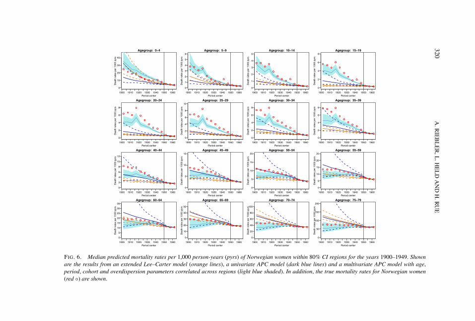
4.2.3. Projections. The median projected death rates per 1,000 person-yearstogether with 80% pointwise prediction intervals for Norwegian women obtainedfrom all three models are shown in Figure 6 for the first half and Figure 7 for thesecond half of the 20th century. Furthermore, the true death rates of Norwegianwomen are added to the figures. For all models and especially for the univariateAPC model, the prediction intervals are getting wider as prediction time goes on.While the projections of the two univariate approaches are almost straight lines,different temporal patterns across age groups can be seen for the correlated model.The Spanish flu was especially well captured by the correlated approach. Since
320A
.RIE
BL
ER
,L.H
EL
DA
ND
H.R
UE
FIG. 6. Median predicted mortality rates per 1,000 person-years (pyrs) of Norwegian women within 80% CI regions for the years 1900–1949. Shownare the results from an extended Lee–Carter model (orange lines), a univariate APC model (dark blue lines) and a multivariate APC model with age,period, cohort and overdispersion parameters correlated across regions (light blue shaded). In addition, the true mortality rates for Norwegian women(red ◦) are shown.
CO
RR
EL
AT
ED
MU
LTIV
AR
IAT
EA
PCM
OD
EL
S321
FIG. 7. Median predicted mortality rates per 1,000 person-years (pyrs) of Norwegian women within 80% CI regions for the years 1950–1999. Shownare the results from an extended Lee–Carter model (orange lines), a univariate APC model (dark blue lines) and a multivariate APC model with age,period, cohort and overdispersion parameters correlated across regions (light blue shaded). In addition, the true mortality rates for Norwegian women(red ◦) are shown.
322 A. RIEBLER, L. HELD AND H. RUE
the Spanish flu did not affect all age groups, this event (also present for Denmarkand Sweden) was captured and transferred to the projections due to the correlatedoverdispersion parameters and not because of the correlated period effects, as onemight intuitively guess. Predicting the second half of the 20th century, the projec-tions of the extended Lee–Carter model agree very well with the true observations.In particular, the rates for ages over 60 are well projected, where the cMAPC modeltends to underestimate the overall death rate.
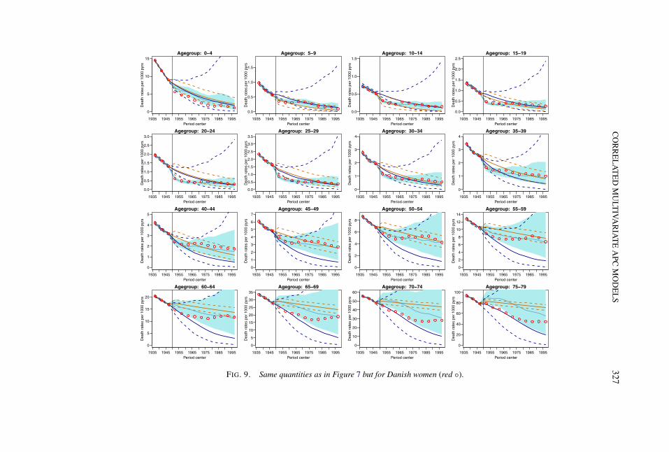
Projections for Danish and Swedish women are shown in Figures 8, 9, 10 and 11in Appendix B. Here, the projections of the correlated approach coincide for allscenarios and all age groups very well with the observed rates. In contrast, theextended Lee–Carter approach tends to underestimate rates for younger age groupswhen predicting the first half, and to overestimate rates for older age groups whenpredicting the second half of the 20th century.
5. Discussion. In this paper we proposed the use of correlated smoothing pri-ors and correlated overdispersion parameters for multivariate Bayesian APC ap-proaches analyzing mortality or morbidity rates stratified by age, period, cohortand one further variate. The specification of correlated smoothing priors involvesa Kronecker product precision structure for the outcome-specific time effects, thatis, age, period and/or cohort effects. We implemented correlated multivariate APCmodels based on a uniform correlation structure in MCMC and INLA. In the firstapplication we analyzed COPD mortality among males in England and Wales us-ing MCMC and INLA, and compared the results of an ordinary multivariate APCmodel with those obtained from different correlated model formulations. A com-parison of MCMC and INLA showed virtually identical results. As indicated bythe log marginal likelihood, the formulation with both correlated overdispersionand correlated stratum-specific period and cohort effects was classified as the best.As shown in the relative risk estimates, the correlated model structure improvedthe precision of the relative risk estimates especially for younger birth cohorts.
In a second application on overall mortality of Danish, Swedish and Norwegianwomen in the 20th century, we performed a cross-prediction study. We illustratedthe good predictive quality of the correlated approach when imputing missing dataunits for one country if these units are available for the other countries. As focuswas set on projections, which are an estimable function in (multivariate) APC mod-els, we were able to consider the most flexible model with country-specific age,period, cohort and overdispersion parameters that were all correlated across coun-tries. In total, we considered six scenarios treating in turn for a particular countryeither the first or second half of the data as missing and subsequently predicting theomitted data units. We compared the projections to those obtained from a univari-ate APC model and a Lee–Carter approach embedded into a quasi-Poisson modelusing the proper Dawid–Sebastiani scoring rule. Since only the correlated formu-lation can take advantage from the complete tables of the remaining two countries,it was classified as the best model in five of the six scenarios. Furthermore, we
CORRELATED MULTIVARIATE APC MODELS 323
observed that the predictive quality stayed almost constant when increasing thenumber of periods to predict, which was not the case for the two univariate ap-proaches. Thus, the correlated approach outperformed both univariate methods inshort and long-term projections.
In real life, long-term projections of mortality or disease rates into the futureare difficult to make using our proposed approach, since there will be no datafrom comparable time-series available. For short-term predictions, data for somestrata may be already available, while for others they are still missing. Here, thecorrelation approach will be useful to forecast the missing units.
For the simultaneous projection of several strata, Li and Lee (2005) extendedthe original log-linear Lee–Carter model. In the simplest extension, they assignedeach stratum its own age pattern, while assuming shared age-specific patterns ofmortality change and a shared time trend. Future values are then predicted for theshared time trend based on an ARIMA process. Incorporating both shared andstratum-specific parameters, this model seems to be similar in spirit to an uncor-related multivariate APC model [Riebler and Held (2010)]. In a more complexmodel, Li and Lee (2005) included an additional stratum-specific bilinear term toallow for differences between the rate of change in mortality in a particular stratumand the rate of change implied by the common bilinear term. However, in contrastto the correlated approach presented here, those extensions cannot take advantageof data units missing in one stratum but present for the remaining. By contrast, ourapproach could be equally used to impute data for all strata simultaneously, ben-efitting from the periods where complete data existed. Furthermore, we can usestratum-specific effects for all parameters. Information from the remaining stratais borrowed by incorporating correlation. In a Bayesian setting the inclusion of cor-relation between parameters is straightforward via the prior distributions, whereasin a frequentist setting this seems to be more complex.
Another interesting field of application is similar in spirit to the inference oncollapsed margins, proposed by Byers and Besag (2000). In the context of col-lapsed margins, complete data are available on several risk factors, but a subse-quent analysis indicates that information on an additional variable is relevant. Forthis variable the numbers of persons at risk are available but not the numbers ofcases. Byers and Besag (2000) propose a Bayesian approach to estimate the ef-fect of the variable. In multivariate APC models it might be that multiple datasets are only available for a specific period in time, while, before and/or after thisdate, data only exist for the conjunction of outcomes. A typical example could beGermany, which was formerly united, then separated and now united again. Usingage-specific data on the population sizes from 1990 up to now for East and WestGermany separately, it may be possible to project mortality rates for both individ-ual parts, by exploiting the correlation present when they were divided. Thus, theobservations for the conjunction of both parts could be separated. However, furtherinvestigations are required to explore the applicability.
324 A. RIEBLER, L. HELD AND H. RUE
The proposed methodology can only be applied to data stratified by one furthervariate. For analyzing mortality rates stratified by more than one further variate,a conditional approach using a multinomial logistic regression model has beenproposed [Held and Riebler (2011)]. However, the incorporation of correlation hasnot yet been considered.
A disadvantage of the proposed methodology might be that it is essentially ad-ditive in age, period and cohort, so that interactions between the time dimensionscannot be explicitly modeled. Currie, Durban and Eilers (2004) proposed two-dimensional smoothing to address this problem in the analysis of an individualregistry data set. Biatat and Currie (2010) started to extend this work and pro-posed a model to compare various mortality tables by assuming a common two-dimensional P-spline surface and additional one-dimensional smoothing functionsfor age and period.
In general, the use of a Kronecker product structure is a promising area forfurther research, as different correlation structures can easily be combined withdifferent precision matrices. Based on the uniform correlation structure INLA can,by now, correlate a wide range of other GMRF models as components of more gen-eral additive regression models. Examples are as follows: nonparametric seasonalmodels, continuous-time random walks or models with a user specified precisionmatrix. However, the uniform correlation structure is rather restrictive and mayonly be plausible for a few outcomes. Future work encompasses the integrationof other correlation structures, for example, depending on the distance betweenunits, so that the approach can be extended to the space–time context, for example.Furthermore, we are investigating the use of correlated two-dimensional smooth-ing priors in INLA to incorporate interactions between time-dimensions into themultivariate APC model.
APPENDIX A: UNIFORM CORRELATION STRUCTURE
Let C be an R ×R correlation matrix with uniform correlation structure, so thatC = (1 − ρ)I + ρJ:
C =
⎛⎜⎜⎜⎜⎝
1 ρ · · · ρ
ρ. . .
. . ....
.... . .
. . . ρ
ρ · · · ρ 1
⎞⎟⎟⎟⎟⎠ ,
where ρ is the correlation parameter, I denotes the R × R identity matrix and J anR × R matrix of ones. Then the inverse C−1 is given by
C−1 =
⎛⎜⎜⎜⎝
a b · · · b
b. . .
. . ....
.... . .
. . . b
b · · · b a
⎞⎟⎟⎟⎠
CORRELATED MULTIVARIATE APC MODELS 325
with
a = − (R − 2) · ρ + 1
(ρ − 1){(R − 1) · ρ + 1} ,
b = ρ
(ρ − 1){(R − 1) · ρ + 1} .
PROOF. If C−1C = I, then C−1 is the inverse of C. For the diagonal elementsof C−1C it follows that
(C−1C)(i,i) = a + (R − 1) · b · ρ
= −(R − 2) · ρ − 1 + (R − 1) · ρ2
(ρ − 1){(R − 1) · ρ + 1}
= −Rρ + 2ρ − 1 + Rρ2 − ρ2
Rρ2 − ρ2 − Rρ + ρ + ρ − 1= 1
for all i = 1, . . . ,R. For the nondiagonal elements, that is, i �= j , we get
(C−1C)(i,j) = a · ρ + b + (R − 2) · b · ρ
= {−(R − 2) · ρ − 1}ρ + ρ + (R − 2) · ρ2
(ρ − 1){(R − 1) · ρ + 1}
= −Rρ2 + 2ρ2 − ρ + ρ + Rρ2 − 2ρ2
(ρ − 1){(R − 1) · ρ + 1} = 0. �
The determinant |C−1| is given by
|C−1| = |C|−1 = [(1 + (R − 1)ρ
)(1 − ρ)R−1]−1
.
PROOF. We show that |C| = (1 + (R − 1)ρ)(1 − ρ)R−1, as the inverse casefollows immediately. Remember that |C| = |I − ρI + ρJ|. The identity matrix hasR times the eigenvalue 1. The matrix J has once the eigenvalue R and R − 1 timesthe eigenvalue 0. Since both matrices (I and J) share the same eigenvectors, theeigenvalues for C are (1 − ρ + ρ · R) and (1 − ρ) with multiplicity R − 1, so thatthe determinant of C, the product of the eigenvalues, is
|C| = (1 − ρ + ρ · R)(1 − ρ)R−1 = (1 + (R − 1)ρ
)(1 − ρ)R−1. �
APPENDIX B: PROJECTION FOR DENMARK AND SWEDEN
The median projected death rates per 1,000 person-years together with 80%pointwise prediction intervals for Danish and Swedish women obtained from allthree models are shown in Figures 8 and 10 for the first half and Figures 9 and 11for the second half of the 20th century.
326A
.RIE
BL
ER
,L.H
EL
DA
ND
H.R
UE
FIG. 8. Same quantities as in Figure 6 but for Danish women (red ◦).
CO
RR
EL
AT
ED
MU
LTIV
AR
IAT
EA
PCM
OD
EL
S327FIG. 9. Same quantities as in Figure 7 but for Danish women (red ◦).
328A
.RIE
BL
ER
,L.H
EL
DA
ND
H.R
UE
FIG. 10. Same quantities as in Figure 6 but for Swedish women (red ◦).
CO
RR
EL
AT
ED
MU
LTIV
AR
IAT
EA
PCM
OD
EL
S329FIG. 11. Same quantities as in Figure 7 but for Swedish women (red ◦).
330 A. RIEBLER, L. HELD AND H. RUE
Acknowledgments. We would like to thank the Editor and referees for theirhelpful comments and suggestions that improved the paper.
SUPPLEMENTARY MATERIAL
Code repository for the cross-prediction study of overall mortality ofScandinavian women (DOI: 10.1214/11-AOAS498SUPP; .zip). This repositoryarchives the data, R-code and results for the cross-prediction study of overall mor-tality of Scandinavian women presented in Section 4.2. In particular, it containscode to make Table 1 and Figures 5–11.
REFERENCES
ANDREASEN, V., VIBOUD, C. and SIMONSEN, L. (2008). Epidemiologic characterization of the1918 influenza pandemic summer wave in Copenhagen: Implications for pandemic control strate-gies. J. Infect. Dis. 197 270–278.
ARMITAGE, P. (1966). The chi-square test for heterogeneity of proportions, after adjustment forstratification. J. Roy. Statist. Soc. Ser. B 28 150–163. MR0196851
BAKER, A. and BRAY, I. (2005). Bayesian projections: What are the effects of excluding data fromyounger age groups? Am. J. Epidemiol. 162 798–805.
BERZUINI, C. and CLAYTON, D. (1994). Bayesian analysis of survival on multiple time scales. Stat.Med. 13 823–838.
BESAG, J., GREEN, P., HIGDON, D. and MENGERSEN, K. (1995). Bayesian computation andstochastic systems. Statist. Sci. 10 3–66. MR1349818
BIATAT, V. D. and CURRIE, I. D. (2010). Joint models for classification and comparison of mortalityin different countries. In 25th International Workshop on Statistical Modelling (A. W. Bowman,ed.) 89–94. Univ. Glasgow, UK.
BILLINGSLEY, P. (1986). Probability and Measure, 2nd ed. Wiley, New York. MR0830424BOOTH, H. (2006). Demographic forecasting: 1980 to 2005 in review. International Journal of Fore-
casting 22 547–581.BOOTH, H., MAINDONALD, J. and SMITH, L. (2002). Applying Lee–Carter under conditions of
variable mortality decline. Popul. Stud. (Camb.) 56 325–336.BOOTH, H., HYNDMAN, R. J., TICKLE, L. and DE JONG, P. (2006). Lee–Carter mortality forecast-
ing: A multi-country comparison of variants and extensions. Demographic Research 15 289–310.BOUCHARDY, C., LUTZ, J.-M. and KÜHNI, C. (2011). Krebs in der Schweiz: Stand und Entwick-
lung von 1983 bis 2007. BFS, NICER, SKKR, Neuchâtel.BRAY, I. (2002). Application of Markov chain Monte Carlo methods to projecting cancer incidence
and mortality. J. Roy. Statist. Soc. Ser. C 51 151–164. MR1900163BRAY, I., BRENNAN, P. and BOFFETTA, P. (2001). Recent trends and future projections of lymphoid
neoplasms—a Bayesian age-period-cohort analysis. Cancer Causes and Control 12 813–820.BRILLINGER, D. R. (1986). The natural variability of vital rates and associated statistics. Biometrics
42 693–734. MR0872958BROUHNS, N., DENUIT, M. and VERMUNT, J. K. (2002). A Poisson log-bilinear regression
approach to the construction of projected lifetables. Insurance Math. Econom. 31 373–393.MR1945540
BUTT, Z. and HABERMAN, S. (2009). ilc: A collection of R functions for fitting a class of Lee–Carter mortality models using iterative fitting algorithms. Technical report, Actuarial ResearchPaper No. 190, City Univ. London, UK.
BYERS, S. and BESAG, J. (2000). Inference on a collapsed margin in disease mapping. Stat. Med.19 2243–2249.
CARLIN, B. P. and BANERJEE, S. (2003). Hierarchical multivariate CAR models for spatio-temporally correlated survival data. In Bayesian Statistics, 7 (Tenerife, 2002) (J. M. Bernardo,M. J. Bayarri, J. O. Berger, A. P. Dawid, D. Heckerman and A. F. M. Smith, eds.) 45–63. OxfordUniv. Press, New York. MR2003166
CLAYTON, D. and SCHIFFLERS, E. (1987). Models for temporal variation in cancer rates. II: Age-period-cohort models. Stat. Med. 6 469–481.
CURRIE, I. D., DURBAN, M. and EILERS, P. H. C. (2004). Smoothing and forecasting mortalityrates. Stat. Model. 4 279–298. MR2086492
CZADO, C., GNEITING, T. and HELD, L. (2009). Predictive model assessment for count data. Bio-metrics 65 1254–1261. MR2756513
DOCKERY, D. W. and POPE, C. A. (1994). Acute respiratory effects of particulate air pollution.Annu. Rev. Public Health 15 107–132.
ESS, S., SAVIDAN, A., FRICK, H., RAGETH, C., VLASTOS, G., LÜTOLF, U. and THÜRLI-MANN, B. (2010). Geographic variation in breast cancer care in Switzerland. Cancer Epidemiol.34 116–121.
FAHRMEIR, L. and TUTZ, G. (2001). Multivariate Statistical Modelling Based on Generalized Lin-ear Models, 2nd ed. Springer, New York. MR1832899
FIENBERG, S. E. and MASON, W. M. (1979). Identification and estimation of age-period-cohortmodels in the analysis of discrete archival data. Sociological Methodology 10 1–67.
FISHER, R. A. (1958). Statistical Methods for Research Workers, 13th (rev.) ed. Oliver and Boyd,Edinburgh.
FU, W. J. J. (2000). Ridge estimator in singular design with application to age-period-cohort analysisof disease rates. Comm. Statist. Theory Methods 29 263–278.
GELFAND, A. E. and GHOSH, S. K. (1998). Model choice: A minimum posterior predictive lossapproach. Biometrika 85 1–11. MR1627258
GELFAND, A. E. and VOUNATSOU, P. (2003). Proper multivariate conditional autoregressive mod-els for spatial data analysis. Biostatistics 4 11–25.
GNEITING, T. and RAFTERY, A. E. (2007). Strictly proper scoring rules, prediction, and estimation.J. Amer. Statist. Assoc. 102 359–378. MR2345548
GRECO, F. P. and TRIVISANO, C. (2009). A multivariate CAR model for improving the estimationof relative risks. Stat. Med. 28 1707–1724. MR2675246
HANSELL, A. L. (2004). The epidemiology of chronic obstructive pulmonary disease in the UK:spatial and temporal variations. Ph.D. thesis, Faculty of Medicine, Univ. London, Imperial Col-lege, St Mary’s Campus.
HANSELL, A., KNORR-HELD, L., BEST, N., SCHMID, V. and AYLIN, P. (2003). COPD mortal-ity trends 1950–1999 in England and Wales—Did the 1956 Clean Air Act make a detectabledifference? Epidemiology 14 S55.
HARVEY, A. (1990). Forecasting, Structural Time Series Models and the Kalman Filter, Reprinteded. Cambridge Univ. Press, Cambridge.
HELD, L. and RIEBLER, A. (2011). A conditional approach for inference in multivariate age-period-cohort models. Stat. Methods Med. Res. To appear. DOI:10.1177/0962280210379761.
HEUER, C. (1997). Modeling of time trends and interactions in vital rates using restricted regressionsplines. Biometrics 53 161–177.
HOLFORD, T. R. (1983). The estimation of age, period and cohort effects for vital rates. Biometrics39 311–324. MR0714415
HOLFORD, T. R. (1992). Analysing the temporal effects of age, period and cohort. Stat. MethodsMed. Res. 1 317–337.
HOLFORD, T. R. (2006). Approaches to fitting age-period-cohort models with unequal intervals.Stat. Med. 25 977–993. MR2225187
HUMAN MORTALITY DATABASE (2011). Univ. California, Berkeley (USA), and MaxPlanck Institute for Demographic Research (Germany). Available at www.mortality.org orwww.humanmortality.de.
JACOBSEN, R., VON EULER, M., OSLER, M., LYNGE, E. and KEIDING, N. (2004). Women’sdeath in Scandinavia—what makes Denmark different? European Journal of Epidemiology 19117–121.
KAZEROUNI, N., ALVERSON, C. J., REDD, S. C., MOTT, J. A. and MANNINO, D. M. (2004). Sexdifferences in COPD and lung cancer mortality trends—United States, 1968–1999. J. Women’sHealth 13 17–23.
KNORR-HELD, L. (2000). Bayesian modelling of inseparable space–time variation in disease risk.Stat. Med. 19 2555–2567.
KNORR-HELD, L. and RAINER, E. (2001). Projections of lung cancer mortality in West Germany:A case study in Bayesian prediction. Biostatistics 2 109–129.
KOLTE, I. V., SKINHØJ, P., KEIDING, N. and LYNGE, E. (2008). The Spanish flu in Denmark.Scand. J. Infect. Dis. 40 538–546.
KONISHI, S. (1985). Normalizing and variance stabilizing transformations for intraclass correlations.Ann. Inst. Statist. Math. 37 87–94. MR0790377
KUANG, D., NIELSEN, B. and NIELSEN, J. P. (2008). Identification of the age-period-cohort modeland the extended chain-ladder model. Biometrika 95 979–986. MR2461224
LAGAZIO, C., BIGGERI, A. and DREASSI, E. (2003). Age-period-cohort models and disease map-ping. Environmetrics 14 475–490.
LEE, R. D. and CARTER, L. R. (1992). Modeling and forecasting U.S. mortality. J. Amer. Statist.Assoc. 87 659–671.
LEHMANN, E. L. (1999). Elements of Large-Sample Theory. Springer, New York. MR1663158LEVI, F., RANDIMBISON, L., TE, V. C., ROLLAND-PORTAL, I., FRANCESCHI, S. and LA VEC-
CHIA, C. (1993). Multiple primary cancers in the Vaud cancer registry, Switzerland, 1974-89. Br.J. Cancer 67 391–395.
LEVI, F., LA VECCHIA, C., RANDIMBISON, L., ERLER, G., TE, V. C. and FRANCESCHI, S.(1998). Incidence, mortality and survival from prostate cancer in Vaud and Neuchâtel, Switzer-land, 1974–1994. Ann. Oncol. 9 31–35.
LEVI, F., RANDIMBISON, L., TE, V.-C. and LA VECCHIA, C. (2002). Thyroid cancer in Vaud,Switzerland: An update. Thyroid 12 163–168.
LI, N. and LEE, R. (2005). Coherent mortality forecasts for a group of populations: An extension ofthe Lee–Carter method. Demography 42 575–594.
LINDLEY, D. (1965). Introduction to Probability and Statistics from a Bayesian Viewpoint, Part 2,Inference. Cambridge Univ. Press, Cambridge.
MARDIA, K. (1988). Multi-dimensional multivariate Gaussian Markov random fields with applica-tion to image processing. J. Multivariate Anal. 24 265–284.
NAKAMURA, T. (1986). Bayesian cohort models for general cohort table analyses. Ann. Inst. Statist.Math. 38 353–370.
OGATA, Y., KATSURA, K., KEIDING, N., HOLST, C. and GREEN, A. (2000). Empirical Bayesage-period-cohort analysis of retrospective incidence data. Scand. J. Stat. 27 415–432.
OSMOND, C. and GARDNER, M. J. (1982). Age, period and cohort models applied to cancer mor-tality rates. Stat. Med. 1 245–259.
PAUL, M., RIEBLER, A., BACHMANN, L. M., RUE, H. and HELD, L. (2010). Bayesian bivariatemeta-analysis of diagnostic test studies using integrated nested Laplace approximations. Stat.Med. 29 1325–1339. MR2757228
R DEVELOPMENT CORE TEAM (2010). R: A Language and Environment for Statistical Computing.R Foundation for Statistical Computing, Vienna, Austria.
RIEBLER, A. and HELD, L. (2010). The analysis of heterogeneous time trends in multivariate age-period-cohort models. Biostatistics 11 57–69.
RIEBLER, A., HELD, L. and RUE, H. (2011). Supplement to “Estimation and extrapolation oftime trends in registry data—Borrowing strength from related populations.” DOI:10.1214/11-AOAS498SUPP.
RIEBLER, A., HELD, L., RUE, H. and BOPP, M. (2011). Gender-specific differences and the impactof family integration on time trends in age-stratified Swiss suicide rates. J. Roy. Statist. Soc. Ser. A.To appear.
ROBERTSON, C. and BOYLE, P. (1986). Age, period and cohort models: The use of individualrecords. Stat. Med. 5 527–538.
RUE, H. and HELD, L. (2005). Gaussian Markov Random Fields: Theory and Applications. Mono-graphs on Statistics and Applied Probability 104. Chapman and Hall/CRC, Boca Raton, FL.MR2130347
RUE, H., MARTINO, S. and CHOPIN, N. (2009). Approximate Bayesian inference for latent Gaus-sian models by using integrated nested Laplace approximations. J. R. Stat. Soc. Ser. B Stat.Methodol. 71 319–392. MR2649602
SCHMID, V. and HELD, L. (2004). Bayesian extrapolation of space-time trends in cancer registrydata. Biometrics 60 1034–1042. MR2133556
SCHMID, V. J. and HELD, L. (2007). Bayesian age-period-cohort modeling and prediction—BAMP.Journal of Statistical Software 21 1–15.
SCHRÖDLE, B., HELD, L., RIEBLER, A. and DANUSER, J. (2011). Using integrated nested Laplaceapproximations for the evaluation of veterinary surveillance data from Switzerland: A case study.J. R. Stat. Soc. Ser. C. Appl. Stat. 60 261–279.
SUNYER, J. (2001). Urban air pollution and chronic obstructive pulmonary disease: A review. Eur.Respir. J. 17 1024–1033.
VERKOOIJHEN, H. M., FIORETTA, G., VLASTOS, G., MORABIA, A., SCHUBERT, H., SAP-PINO, A., PELTE, M., SCHAFER, P., KURTZ, J. and BOUCHARDY, C. (2003). Important in-crease of invasive lobular breast cancer incidence in Geneva, Switzerland. International Journalof Cancer 104 778–781.
YANG, Y., FU, W. J. and LAND, K. C. (2004). A methodological comparison of age-period-cohortmodels: The intrinsic estimator and conventional generalized linear models. Sociological Method-ology 34 75–110.