Page 1
PO 0809
Estimation, Detection, and Identification Graduate Course on the
CMU/Portugal ECE PhD Program Spring 2008/2009
Chapter 3 Cramer-Rao Lower Bounds
Instructor: Prof. Paulo Jorge Oliveira
pjcro @ isr.ist.utl.pt Phone: +351 21 8418053 ou 2053 (inside IST)
Page 2
PO 0809
Syllabus: Classical Estimation Theory
…
Chap. 2 - Minimum Variance Unbiased Estimation [1 week]
Unbiased estimators; Minimum Variance Criterion; Extension to vector parameters;
Efficiency of estimators;
Chap. 3 - Cramer-Rao Lower Bound [1 week] Estimator accuracy; Cramer-Rao lower bound (CRLB); CRLB for signals in white Gaussian noise; Examples;
Chap. 4 - Linear Models in the Presence of Stochastic Signals [1 week]
Stationary and transient analysis; White Gaussian noise and linear systems; Examples;
Sufficient Statistics; Relation with MVU Estimators;
continues…
Page 3
PO 0809
Estimator accuracy: The accuracy on the estimates dependents very much on the PDFs
Example (revisited):
Model of signal
Observation PDF
for a disturbance N(0, σ2)
Remarks:
If σ2 is Large then the performance of the estimator is Poor;
If σ2 is Small then the performance of the estimator is Good; or
-100 -80 -60 -40 -20 0 20 40 60 80 100 0.005 0.01 0.015 0.02 0.025 0.03 0.035
x[0]
p(x[
0]; q )
-100 -80 -60 -40 -20 0 20 40 60 80 100 1.5 2
2.5 3
3.5 x 10 -3
x[n]
p(x[
0]; q )
If PDF concentration is High then the parameter accuracy is High.
How to measure sharpness of PDF (or concentration)?
Page 4
PO 0809
Estimator accuracy: When PDFs are seen as function of the unknown parameters, for x fixed, they are called
as Likelihood function. To measure the sharpness note that (and ln is monotone…)
Its first and second derivatives are respectively:
As we know that the estimator  has variance σ2 (at least for this example)
We are now ready to present an important theorem…
∂∂A
ln p x[0]; A( ) = 1σ 2 x[0]− A( ) and
−
∂2
∂A2 ln p x[0]; A( ) = 1σ 2 .
Page 5
PO 0809
Cramer-Rao lower bound: Theorem 3.1 (Cramer-Rao lower bound, scalar parameter) – It is assumed that the
PDF p(x; θ) satisfies the “regularity” condition
(1)
where the expectation is taken with respect to p(x; θ). Then, the variance of any unbiased
estimator must satisfy
(2)
where the derivative is evaluated at the true value of θ and the expectation is taken with
respect to p(x, θ). Furthermore, an unbiased estimator can be found that attains the bound
for all θ if and only if
(3)
for some functions g(.) and I (.). The estimator, which is the MVU estimator, is
and the minimum variance 1/ I(θ).
E ∂
∂θln p x;θ( )⎡
⎣⎢
⎤
⎦⎥ = 0 forall θ
var θ( ) ≥ 1
−E ∂2
∂θ 2 ln p x;θ( )⎡
⎣⎢
⎤
⎦⎥
θ
∂∂θ
ln p x;θ( ) = I θ( ) g x( ) −θ( ) θ = g x( ),
Page 6
PO 0809
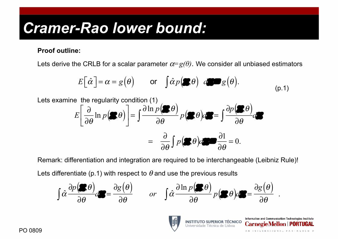
Cramer-Rao lower bound: Proof outline:
Lets derive the CRLB for a scalar parameter α=g(θ). We consider all unbiased estimators
(p.1)
Lets examine the regularity condition (1)
Remark: differentiation and integration are required to be interchangeable (Leibniz Rule)!
Lets differentiate (p.1) with respect to θ and use the previous results
E α⎡⎣ ⎤⎦ = α = g θ( ) or α p x ;θ( )∫ dx = g θ( ).
E ∂∂θ
ln p x ;θ( )⎡
⎣⎢
⎤
⎦⎥ =
∂ ln p x ;θ( )∂θ
p x ;θ( )∫ dx =∂p x ;θ( )
∂θ∫ dx
=∂∂θ
p x ;θ( )∫ dx = ∂1∂θ
= 0.
α∂p x ;θ( )
∂θ∫ dx =∂g θ( )∂θ
or α∂ ln p x ;θ( )
∂θp x ;θ( )∫ dx =
∂g θ( )∂θ
.
Page 7
PO 0809
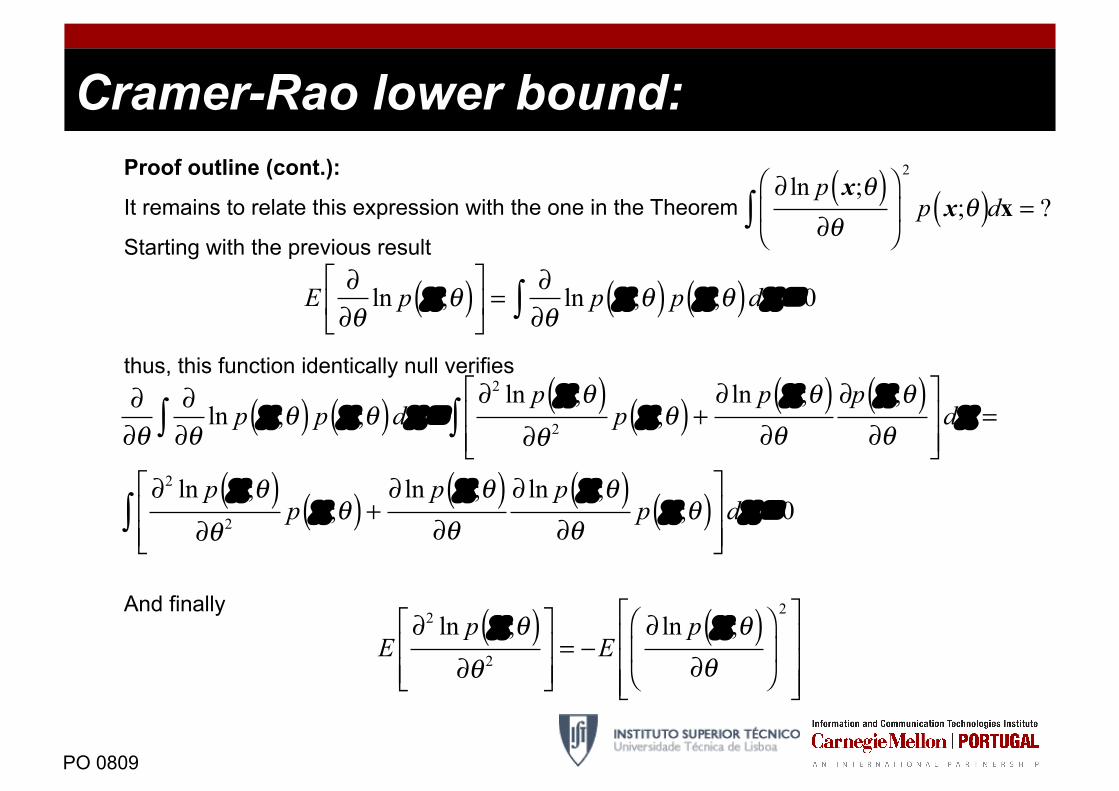
Cramer-Rao lower bound: Proof outline (cont.):
This can be modified to
as
Now applying the Cauchy-Schwarz inequality
considering
results
α − α( ) ∂ ln p x ;θ( )
∂θp x ;θ( )∫ dx =
∂g θ( )∂θ
,
α∂ ln p x;θ( )
∂θp x;θ( )∫ dx = αE
∂ ln p x;θ( )∂θ
⎡
⎣⎢⎢
⎤
⎦⎥⎥= 0.
Page 8
PO 0809
Cramer-Rao lower bound: Proof outline (cont.):
It remains to relate this expression with the one in the Theorem
Starting with the previous result
thus, this function identically null verifies
And finally
∂ ln p x;θ( )∂θ
⎛
⎝⎜
⎞
⎠⎟
2
p x;θ( )∫ dx = ?
E ∂
∂θln p x ;θ( )⎡
⎣⎢
⎤
⎦⎥ =
∂∂θ
ln p x ;θ( ) p x ;θ( )dx =∫ 0
∂∂θ
∂∂θ
ln p x ;θ( ) p x ;θ( )dx =∫∂2 ln p x ;θ( )
∂θ 2 p x ;θ( ) + ∂ ln p x ;θ( )∂θ
∂p x ;θ( )∂θ
⎡
⎣⎢⎢
⎤
⎦⎥⎥
dx∫ =
∂2 ln p x ;θ( )∂θ 2 p x ;θ( ) + ∂ ln p x ;θ( )
∂θ∂ ln p x ;θ( )
∂θp x ;θ( )
⎡
⎣⎢⎢
⎤
⎦⎥⎥
dx =∫ 0
E∂2 ln p x ;θ( )
∂θ 2
⎡
⎣⎢⎢
⎤
⎦⎥⎥= −E
∂ ln p x ;θ( )∂θ
⎛
⎝⎜
⎞
⎠⎟
2⎡
⎣
⎢⎢⎢
⎤
⎦
⎥⎥⎥
Page 9
PO 0809
Cramer-Rao lower bound: Proof outline (cont.):
Taking this into consideration, i.e.
expression (2) results, in the case where g(θ)=θ.
The result (3) will be obtained next…
See also appendix 3.B for the derivation in the vector case.
Page 10
PO 0809
Cramer-Rao lower bound: Summary:
• Being able to place a lower bound on the variance of any unbiased
estimator is very useful.
• It allow us to assert that an estimator is the MVU estimator (if it
attains the bound for all values of the unknown parameter).
• It provides in all cases a benchmark for the unbiased estimators that
we can design.
• It alerts to impossibility of finding unbiased estimators with variance
lower than the bound.
• Provides a systematic way of finding the MVU estimator, if it exists
and if an extra condition is verified.
Page 11
PO 0809
Example: Example (DC level in white Gaussian noise):
Problem: Find MVU estimator. Approach: Compute CRLB, if right form we have it.
Signal model:
Likelihood function:
CRLB:
The estimator is unbiased and has the same variance, thus it is a MVU estimator! And it
has the form:
∂∂A
ln p x; A( ) = ∂∂A
−1
2σ 2 x[n]− A( )2
n=0
N −1∑⎛⎝⎜
⎞⎠⎟=
1σ 2 x[n]− A( ) =n=0
N −1∑ Nσ 2 x − A( )
∂∂A
ln p x; A( ) = I θ( ) g x( ) −θ( ), for I θ( ) = Nσ 2 g x( ) = x.
Page 12
PO 0809
Cramer-Rao lower bound: Proof outline (second part of the theorem):
Still remains to prove that the CRLB is attained for the estimator
If
differentiation relative to the parameter gives
and then
i.e. the bound is attained.
Page 13
PO 0809
Example: Example (phase estimation):
Signal model:
Likelihood function:
−E ∂2
∂φ 2 ln p x;φ( )⎡
⎣⎢
⎤
⎦⎥ = −
A2
σ 2
12−
12
cos 4π f0n + 2φ( )⎛⎝⎜
⎞⎠⎟n=0
N −1∑ ≈NA2
2σ 2
Page 14
PO 0809
Example: Example (phase estimation cont.):
as
for large N.
• Bound decreases as SNR=A2/2σ2 increases
• Bound decreases as N increases
Does an efficient estimator exists? Does a MVUE estimator exists?
−E ∂2
∂φ 2 ln p x |φ( )⎡
⎣⎢
⎤
⎦⎥ = −
A2
σ 2
12−
12
cos 4π f0n + 2φ( )⎛⎝⎜
⎞⎠⎟n=0
N −1∑ ≈NA2
2σ 2
cos 4π f0n + 2φ( ) ≈ 0 for f0 not near 0 or 1/2.
n=0
N −1∑
Page 15
PO 0809
Fisher information: We define the Fisher Information (Matrix) as
Note:
• I(q) ≥0
• It is additive for independent observations
• If identically distributed (same PDF for each x[n])
As N->∞, for iid => CRLB-> 0
I θ( ) = −E ∂2
∂θ 2 ln p x;θ( )⎡
⎣⎢
⎤
⎦⎥ = − E ∂2
∂θ 2 ln p x n⎡⎣ ⎤⎦;θ( )⎡
⎣⎢
⎤
⎦⎥n=0
N −1∑
Page 16
PO 0809
Other estimator characteristic: Efficiency:
An estimator that is unbiased and attains the
CRLB is said to be efficient. CRLB
CRLB CRLB
Page 17
PO 0809
Transformation of parameters: Imagine that the CRLB is known for the parameter θ. Can we compute easily the CRLB
for a linear transformation of the form α = g(θ) = aθ + b ?
Linear transformations preserve biasness and efficiency.
And for a nonlinear transformation of the form α=g(θ)?
α = aθ + b, E aθ + b⎡⎣ ⎤⎦ = aE θ⎡⎣ ⎤⎦ + b = α
Page 18
PO 0809
Transformation of parameters: Remark: after a nonlinear transformation, the good properties can be lost.
Example: Suppose that given a stochastic variable we desire to have
an estimator for α=g(A)=A2 (power estimator). Note that
A bias estimate results. Efficiency is lost.
Page 19
PO 0809
Cramer-Rao lower bound: Theorem 3.1 (Cramer-Rao lower bound, Vector parameter) – It is assumed that the
PDF p(x;θ) satisfies the “regularity” condition
where the expectation is taken with respect to p(x, θ). Then, the variance of any unbiased
estimator must satisfy
where ≥ is interpreted as meaning the matrix is positive semi-definite. The Fisher
information matrix I(θ) is given as
where the derivatives are evaluated at the true value of θ and the expectation is taken
with respect to p(x;θ). Furthermore, an unbiased estimator may be found that attains the
bound for all θ if and only if
(3)
for some functions p dimensional function g(.) and some p x p matrix I (.). The estimator,
which is the MVU estimator, is and its covariance matrix is I-1(θ).
θ
Page 20
PO 0809
Vector Transformation of parameters: The vector transformation of parameters impacts on the CRLB computation as
where the Jacobian is
In the Gaussian general case for x[n]=s[n]+w[n], where
the Fisher information matrix is
Cα −
∂g θ( )∂θ
I −1 θ( ) ∂g θ( )T
∂θ≥ 0
∂g θ( )∂θ
=
∂g1 θ( )∂θ1
...∂g1 θ( )∂θ p
... ... ...∂gr θ( )∂θ1
∂gr θ( )∂θ p
⎡
⎣
⎢⎢⎢⎢⎢⎢⎢
⎤
⎦
⎥⎥⎥⎥⎥⎥⎥
w N µ θ( ),Cθ( )
Page 21
PO 0809
Example: Example (line fitting):
Signal model:
Likelihood function:
The Fisher Information Matrix is
where
p x;θ( ) = 1
(2πσ 2 )N2
e−
1
2σ 2x[n]− A−Bn( )2n=0
N−1∑, where θ = A B⎡⎣ ⎤⎦
T
I θ( ) =−E
∂2 ln p x;θ( )∂A2
⎡
⎣⎢⎢
⎤
⎦⎥⎥
−E∂2 ln p x;θ( )
∂A∂B
⎡
⎣⎢⎢
⎤
⎦⎥⎥
−E∂2 ln p x;θ( )
∂B∂A
⎡
⎣⎢⎢
⎤
⎦⎥⎥
−E∂2 ln p x;θ( )
∂B2
⎡
⎣⎢⎢
⎤
⎦⎥⎥
⎡
⎣
⎢⎢⎢⎢⎢⎢
⎤
⎦
⎥⎥⎥⎥⎥⎥
∂ ln p x;θ( )∂A
=1σ 2 x[n]− A− Bn( )n=0
N −1∑ , and∂ ln p x;θ( )
∂B=
1σ 2 x[n]− A− B( )nn=0
N −1∑ .
Page 22
PO 0809
Example: Example (cont.):
Moreover
Since the second order derivatives do not depend on x, we have immediately that
And also,
I θ( ) = 1σ 2
N N (N −1)2
N (N −1)2
N (N −1)(2N −1)6
⎡
⎣
⎢⎢⎢⎢
⎤
⎦
⎥⎥⎥⎥
∂2 ln p x;θ( )∂A2 = −
Nσ 2 ,
∂2 ln p x;θ( )∂A∂B
= −1σ 2 n
n=0
N −1∑ , and∂2 ln p x;θ( )
∂B2 = −1σ 2 n2
n=0
N −1∑ .
I−1 θ( ) = σ 2
2(2N −1)N (N +1)
−6
N (N +1)
−6
N (N +1)12
N (N 2 −1)
⎡
⎣
⎢⎢⎢⎢⎢
⎤
⎦
⎥⎥⎥⎥⎥
,var A( ) ≥ 2(2N −1)
N (N +1)σ 2
var B( ) ≥ 12N (N 2 −1)
σ 2
Page 23
PO 0809
Example: Example (cont.):
Remarks:
For only one parameter to be determined . Thus a general results was
obtained: when more parameters are to be estimated the CRLB always degrades.
Moreover
The parameter B is easier to be determined, as its CRLB decreases with 1/N3. This
means that x[n] is more sensitive to changes in B than changes in A.
Page 24
PO 0809
Bibliography: Further reading
• Harry L. Van Trees, Detection, Estimation, and Modulation Theory, Parts I to IV, John Wiley,
2001.
• J. Bibby, H. Toutenburg, Prediction and Improved Estimation in Linear Models, John Wiley,
1977.
• C.Rao, Linear Statistical Inference and Its Applications, John Wiley, 1973.
• P. Stoica, R. Moses, “On Biased Estimators and the Unbiased Cramer-Rao Lower Bound,”
Signal Process, vol.21, pp. 349-350, 1990.