Abstract In this paper, we study the problem of estimating a multivariate nor-mal covariance matrix with staircase pattern data. Two kinds of parameterizationsin terms of the covariance matrix are used. One is Cholesky decomposition andanother is Bartlett decomposition. Based on Cholesky decomposition of the covari-ance matrix, the closed form of the maximum likelihood estimator (MLE) of thecovariance matrix is given. Using Bayesian method, we prove that the best equi-variant estimator of the covariance matrix with respect to the special group relatedto Cholesky decomposition uniquely exists under the Stein loss. Consequently, theMLE of the covariance matrix is inadmissible under the Stein loss. Our method canalso be applied to other invariant loss functions like the entropy loss and the sym-metric loss. In addition, based on Bartlett decomposition of the covariance matrix,the Jeffreys prior and the reference prior of the covariance matrix with staircasepattern data are also obtained. Our reference prior is different from Berger andYang’s reference prior. Interestingly, the Jeffreys prior with staircase pattern data isthe same as that with complete data. The posterior properties are also investigated.Some simulation results are given for illustration.
Keywords Maximum likelihood estimator · Best equivariant estimator ·Covariance matrix · Staircase pattern data · Invariant Haar measure · Choleskydecomposition · Bartlett decomposition · Inadmissibility · Jeffreys prior ·Reference prior
1 Introduction
Estimating the covariance matrix ��� in a multivariate normal distribution withincomplete data has been brought to statisticians’attention for several decades. It is
X. Sun (B) · D. SunDepartment of Statistics, University of Missouri, Columbia, MO 65211, USAE-mail: [email protected]
212 X. Sun and D. Sun
well-known that the maximum likelihood estimator (MLE) of ��� fromincomplete data with a general missing-data pattern cannot be expressed in closedform. Anderson (1957) listed several general cases where the MLEs of the param-eters can be obtained by using conditional distribution. Among these cases, thestaircase pattern (also called monotone missing-data pattern) is much more attrac-tive because the other listed missing-data patterns do not actually have enoughinformation for estimating the unconstrained covariance matrix. For this pattern,Liu (1993) presents a decomposition of the posterior distribution of ��� under afamily of prior distributions. Jinadasa and Tracy (1992) obtain a complicated formfor the maximum likelihood estimators of the unknown mean and the covariancematrix in terms of some sufficient statistics, which extends the work of Andersonand Olkin (1985). Recently, Kibria, Sun, Zidek and Le (2002) discussed estimat-ing ��� using a generalized inverted Wishart (GIW) prior and applied the result tomapping PM2.5 exposure. Other related references may include Liu (1999), Littleand Rubin (1987), and Brown, Le and Zidek (1994).
In this paper, we consider a general problem of estimating ��� with the staircasepattern data. Two convenient and interesting parameterizations, Cholesky decom-position and Bartlett decomposition, are used. Section 2 describes the model andsetup. In Sect. 3, we consider the Cholesky decomposition of ��� and derive a closedform expression of the MLE of ��� based on a set of sufficient statistics differentfrom those in Jinadasa and Tracy (1992). We also show that the best equivariantestimator of ��� with respect to the lower-triangular matrix group uniquely existsunder the Stein invariant loss function, resulting in the inadmissibility of the MLE.We find a method to compute the best equivariant estimator of ��� analytically. Byapplying Bartlett decomposition of ���, Sect. 4 deals with the Jeffreys prior and areference prior of ���. Surprisingly, the Jeffreys prior of ��� with the staircase patterndata is the same as the usual one with complete data. The reference prior, how-ever, is different from that for complete data given in Yang and Berger (1994). Theproperties of the posterior distributions under both the Jeffreys and the referencepriors are also investigated in this section.
In Sect. 5, an example is given for computing the MLE, the best equivariantestimator and the Bayesian estimator under the Jeffreys prior. Section 6 presentsa Markov Chain-Monte Carlo (MCMC) algorithm for Bayesian computation ofthe posterior under the reference prior. Some numerical comparisons are brieflystudied among the MLE, the best equivariant estimator of the covariance matrixwith respect to the lower-triangular matrix group, the Bayesian estimators underthe Jeffreys prior and the reference prior with respect to the Stein loss. Severalproofs are given in Appendix.
2 The staircase pattern observations and the loss
Assume that the population follows the multivariate normal distribution with mean0 and covariance matrix ���, namely, (X1, X2, . . . , Xp)′ ∼ Np(0, ���). Suppose thatthep variables are divided into k groups Yi = (Xqi−1+1, . . . , Xqi
)′, for i = 1, . . . , k,where q0 = 0 and qi = ∑i
j=1 pi . Rather than obtaining a random sample of thecomplete vector (X1, X2, . . . , Xp) = (Y′
1, . . . , Y′k), we observe independently
the simple random sample of (Y′1, . . . , Y′
i )′ of size ni . We could rewrite these
Estimating a normal covariance matrix 213
observations as the staircase pattern observations,⎧⎪⎪⎨
where mi = ∑ij=1 nj , i = 1, . . . , k. For convenience, let m0 = 0 hereafter. Such
staircase pattern observations are also called monotone samples in Jinadasa andTracy (1992). Write
��� =
⎛
⎜⎜⎝
���11 ���12 · · · ���1k
���21 ���22 · · · ���2k
......
. . ....
���k1 ���k2 · · · ���kk
⎞
⎟⎟⎠ ,
where ���ij is a pi ×pj matrix. The covariance matrix of (Y′1, . . . , Y′
i )′ is given by
���i =
⎛
⎜⎜⎝
���11 ���12 · · · ���1i
���21 ���22 · · · ���2i
......
. . ....
���i1 ���i2 · · · ���ii
⎞
⎟⎟⎠ . (2)
Clearly ���1 = ���11 and the likelihood function of ��� is
L(���) =k∏
i=1
mi∏
j=mi−1+1
1
|���i | 12
× exp
{
−1
2(Y′
j1, . . . , Y′ji)���
−1i (Y′
j1, . . . , Y′ji)
′}
=k∏
i=1
1
|���i |ni2
etr(
− 1
2���−1
i Vi
), (3)
where
Vi =mi∑
j=mi−1+1
⎛
⎜⎝
Yj1...
Yji
⎞
⎟⎠ (Y′
j1, . . . , Y′ji), i = 1, . . . , k. (4)
Clearly (V1, . . . , Vk) are sufficient statistics of ��� and are mutually independent.To estimate ���, we consider the Stein loss
L(���, ���) = tr(������−1) − log |������−1| − p. (5)
This loss function has been commonly used for estimating ��� for a completed sam-ple, for example, Dey and Srinivasan (1985), Haff (1991),Yang and Berger (1994),and Konno (2001).
214 X. Sun and D. Sun
3 The MLE and the best equivariant estimator
3.1 The MLE of ���
For the staircase pattern data, Jinadasa and Tracy (1992) show the closed form ofthe MLE of ��� based on sufficient statistics V1, . . . , Vk . However, the form is quitecomplicated. We will show that the closed form of the MLE of ��� can be easilyobtained by using a Cholesky decomposition, the lower-triangular squared root of��� with positive diagonal elements, i.e.,
��� = ������′, (6)
where ��� has the blockwise form,
��� =
⎛
⎜⎜⎝
���11 0 · · · 0���21 ���22 · · · 0
......
. . ....
���k1 ���k2 · · · ���kk
⎞
⎟⎟⎠ .
Here ���ij is pi × pj , and ���ii is lower triangular with positive diagonal elements.Also, we could define,
���i =
⎛
⎜⎜⎝
���11 0 · · · 0���21 ���22 · · · 0
......
. . ....
���i1 ���i2 · · · ���ii
⎞
⎟⎟⎠ , i = 1, · · · , k. (7)
Note that ���1 = ���11, ���k = ��� and ���i is the Cholesky decomposition of ���i ,i = 1, . . . , k. The likelihood function of ��� is
L(���) =k∏
i=1
|���i���′i |−
ni2
mi∏
j=mi−1+1
× exp
{
−1
2(Y′
j1, . . . , Y′ji)(���i���
′i )
−1(Y′j1, . . . , Y′
ji)′}
. (8)
It is necessary that an estimator of a covariance matrix is indeed positive definite.Fortunately, with a Cholesky decomposition, it will guarantee that the resultingestimator of ��� is positive definite if each diagonal element of the correspondingestimator of ���ii is positive for all i = 1, . . . , k.
Furthermore, we could define another set of sufficient statistics of ���. We firstdefine
⎧⎪⎪⎨
⎪⎪⎩
W111 = ∑mk
j=1 Yj1Y′j1,
Wi11 = ∑mk
j=mi−1+1(Y′j1, . . . , Y′
j,i−1)′(Y′
j1, . . . , Y′j,i−1),
Wi21 = W′i12 = ∑mk
j=mi−1+1 Yji(Y′j1, . . . , Y′
j,i−1),
Wi22 = ∑mk
j=mi−1+1 YjiY′ji ,
(9)
for i = 2, . . . , k.. Next, we define the inverse matrix of ���. i.e., ��� = ���−1. Clearly
Estimating a normal covariance matrix 215
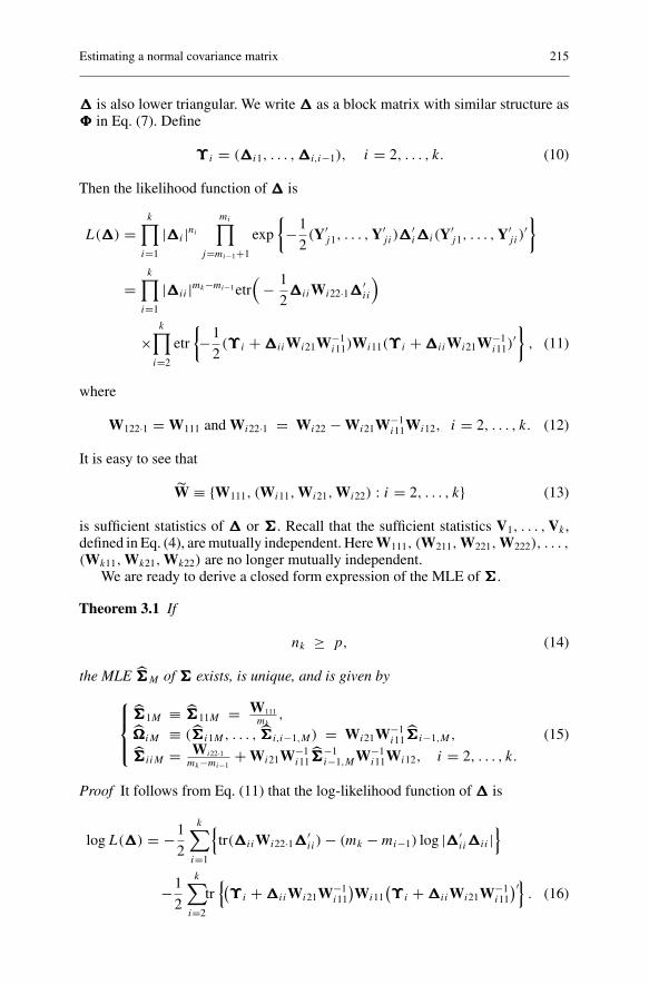
��� is also lower triangular. We write ��� as a block matrix with similar structure as��� in Eq. (7). Define
ϒϒϒi = (���i1, . . . , ���i,i−1), i = 2, . . . , k. (10)
Then the likelihood function of ��� is
L(���) =k∏
i=1
|���i |ni
mi∏
j=mi−1+1
exp
{
−1
2(Y′
j1, . . . , Y′ji)���
′i���i(Y′
j1, . . . , Y′ji)
′}
=k∏
i=1
|���ii |mk−mi−1 etr(
− 1
2���iiWi22·1���′
ii
)
×k∏
i=2
etr
{
−1
2(ϒϒϒi + ���iiWi21W−1
i11)Wi11(ϒϒϒi + ���iiWi21W−1i11)
′}
, (11)
where
W122·1 = W111 and Wi22·1 = Wi22 − Wi21W−1i11Wi12, i = 2, . . . , k. (12)
It is easy to see that
W ≡ {W111, (Wi11, Wi21, Wi22) : i = 2, . . . , k} (13)
is sufficient statistics of ��� or ���. Recall that the sufficient statistics V1, . . . , Vk ,defined in Eq. (4), are mutually independent. Here W111, (W211, W221, W222), . . . ,(Wk11, Wk21, Wk22) are no longer mutually independent.
We are ready to derive a closed form expression of the MLE of ���.
Theorem 3.1 If
nk ≥ p, (14)
the MLE ���M of ��� exists, is unique, and is given by
Proof It follows from Eq. (11) that the log-likelihood function of ��� is
log L(���) = −1
2
k∑
i=1
{tr(���iiWi22·1���′
ii ) − (mk − mi−1) log |���′ii���ii |
}
−1
2
k∑
i=2
tr{(
ϒϒϒi + ���iiWi21W−1i11
)Wi11
(ϒϒϒi + ���iiWi21W−1
i11
)′}. (16)
216 X. Sun and D. Sun
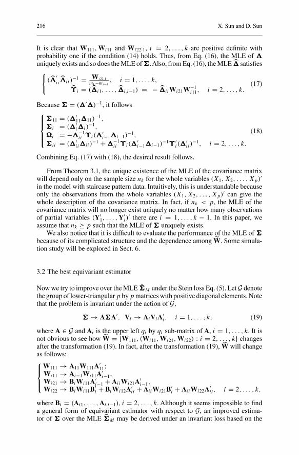
It is clear that W111, Wi11 and Wi22·1, i = 2, . . . , k are positive definite withprobability one if the condition (14) holds. Thus, from Eq. (16), the MLE of ���uniquely exists and so does the MLE of ���.Also, from Eq. (16), the MLE ��� satisfies{
(���′ii���ii)
−1 = Wi22·1mk−mi−1
, i = 1, . . . , k,
ϒϒϒi = (���i1, . . . , ���i,i−1) = − ���iiWi21W−1i11, i = 2, . . . , k.
(17)
Because ��� = (���′���)−1, it follows⎧⎪⎪⎨
⎪⎪⎩
���11 = (���′11���11)
−1,
���i = (���′i���i)
−1,
���i = −���−1ii ϒϒϒi(���
′i−1���i−1)
−1,
���ii = (���′ii���ii)
−1 + ���−1ii ϒϒϒi(���
′i−1���i−1)
−1ϒϒϒ ′i (���
′ii )
−1, i = 2, . . . , k.
(18)
Combining Eq. (17) with (18), the desired result follows.
From Theorem 3.1, the unique existence of the MLE of the covariance matrixwill depend only on the sample size nk for the whole variables (X1, X2, . . . , Xp)′in the model with staircase pattern data. Intuitively, this is understandable becauseonly the observations from the whole variables (X1, X2, . . . , Xp)′ can give thewhole description of the covariance matrix. In fact, if nk < p, the MLE of thecovariance matrix will no longer exist uniquely no matter how many observationsof partial variables (Y′
1, . . . , Y′i )
′ there are i = 1, . . . , k − 1. In this paper, weassume that nk ≥ p such that the MLE of ��� uniquely exists.
We also notice that it is difficult to evaluate the performance of the MLE of ���because of its complicated structure and the dependence among W. Some simula-tion study will be explored in Sect. 6.
3.2 The best equivariant estimator
Now we try to improve over the MLE ���M under the Stein loss Eq. (5). Let G denotethe group of lower-triangular p by p matrices with positive diagonal elements. Notethat the problem is invariant under the action of G,
��� → A���A′, Vi → AiViA′i , i = 1, . . . , k, (19)
where A ∈ G and Ai is the upper left qi by qi sub-matrix of A, i = 1, . . . , k. It isnot obvious to see how W = {W111, (Wi11, Wi21, Wi22) : i = 2, . . . , k} changesafter the transformation (19). In fact, after the transformation (19), W will changeas follows:⎧⎪⎨
⎪⎩
W111 → A11W111A′11;
Wi11 → Ai−1Wi11A′i−1,
Wi21 → BiWi11A′i−1 + AiiWi21A′
i−1,Wi22 → BiWi11B′
i + BiWi12A′ii + AiiWi21B′
i + AiiWi22A′ii , i = 2, . . . , k,
where Bi = (Ai1, . . . , Ai,i−1), i = 2, . . . , k. Although it seems impossible to finda general form of equivariant estimator with respect to G, an improved estima-tor of ��� over the MLE ���M may be derived under an invariant loss based on the
Estimating a normal covariance matrix 217
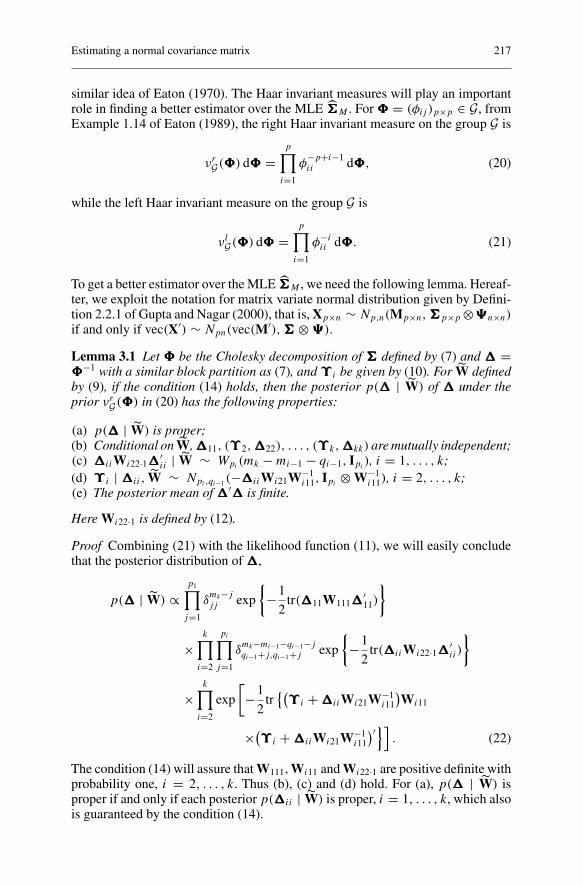
similar idea of Eaton (1970). The Haar invariant measures will play an importantrole in finding a better estimator over the MLE ���M . For ��� = (φij )p×p ∈ G, fromExample 1.14 of Eaton (1989), the right Haar invariant measure on the group G is
νrG(���) d��� =
p∏
i=1
φ−p+i−1ii d���, (20)
while the left Haar invariant measure on the group G is
νlG(���) d��� =
p∏
i=1
φ−iii d���. (21)
To get a better estimator over the MLE ���M , we need the following lemma. Hereaf-ter, we exploit the notation for matrix variate normal distribution given by Defini-tion 2.2.1 of Gupta and Nagar (2000), that is, Xp×n ∼ Np,n(Mp×n, ���p×p ⊗n×n)if and only if vec(X′) ∼ Npn(vec(M′), ��� ⊗ ).
Lemma 3.1 Let ��� be the Cholesky decomposition of ��� defined by (7) and ��� =���−1 with a similar block partition as (7), and ϒϒϒi be given by (10). For W definedby (9), if the condition (14) holds, then the posterior p(��� | W) of ��� under theprior νr
G(���) in (20) has the following properties:
(a) p(��� | W) is proper;(b) Conditional on W, ���11, (ϒϒϒ2, ���22), . . . , (ϒϒϒk, ���kk) are mutually independent;(c) ���iiWi22·1���′
ii | W ∼ Wpi(mk − mi−1 − qi−1, Ipi
), i = 1, . . . , k;(d) ϒϒϒi | ���ii, W ∼ Npi,qi−1(−���iiWi21W−1
i11, Ipi⊗ W−1
i11), i = 2, . . . , k;(e) The posterior mean of ���′��� is finite.
Here Wi22·1 is defined by (12).
Proof Combining (21) with the likelihood function (11), we will easily concludethat the posterior distribution of ���,
p(��� | W) ∝p1∏
j=1
δmk−j
jj exp
{
−1
2tr(���11W111���
′11)
}
×k∏
i=2
pi∏
j=1
δmk−mi−1−qi−1−j
qi−1+j,qi−1+j exp
{
−1
2tr(���iiWi22·1���′
ii )
}
×k∏
i=2
exp
[
−1
2tr{(
ϒϒϒi + ���iiWi21W−1i11
)Wi11
×(ϒϒϒi + ���iiWi21W−1i11
)′}]. (22)
The condition (14) will assure that W111, Wi11 and Wi22·1 are positive definite withprobability one, i = 2, . . . , k. Thus (b), (c) and (d) hold. For (a), p(��� | W) isproper if and only if each posterior p(���ii | W) is proper, i = 1, . . . , k, which alsois guaranteed by the condition (14).
218 X. Sun and D. Sun
For (e), because
���′��� =
⎛
⎜⎜⎜⎝
∑ki=1 ���′
i1���i1∑k
i=2 ���′i1���i2 · · · ���′
k1���kk∑ki=2 ���′
i2���i1∑k
i=2 ���′i2���i2 · · · ���′
k2���kk
......
. . ....
���′kk���k1 ���′
kk���k2 · · · ���′kk���kk
⎞
⎟⎟⎟⎠
, (23)
so the posterior mean of ���′��� is finite if the following three conditions hold:
(i) E(���′ii���ii | W) < ∞, 1 ≤ i ≤ k;
(ii) E(���′ij���ii | W) < ∞, 1 ≤ j < i ≤ k;
(iii) E(���′ij���is | W) < ∞, 1 ≤ j, s < i ≤ k.
To finish the proof of Lemma 3.1, we just need to show (i) because
Here we obtain (24) and (25) by using the result of part (d). From (22), we get
p(���ii | W) ∝pi∏
j=1
δmk−mi−1−qi−1−j
qi−1+j,qi−1+j exp
{
−1
2tr(���iiWi22·1���′
ii
)}
.
Lemma 3 of Sun and Sun (2005) shows that E(���′ii���ii | W) is finite if mk −mi−1 −
qi−1 − j ≥ 0, j = 1, . . . , pi, i = 1, . . . , k, which is equivalent to nk ≥ p.
Because the MLE ���M belongs to a class of G-equivariant estimators, the fol-lowing theorem shows that the best G-equivariant estimator ���B , which is betterthan ���M , uniquely exists.
Theorem 3.2 For the staircase pattern data (1) and under the Stein loss (5), if thecondition (14) holds, the best G-equivariant estimator ���B of ��� exists uniquelyand is given by
���B = {E(���′��� | W)}−1. (26)
Proof For any invariant loss, by Theorem 6.5 in Eaton (1989), the best equivariantestimator of ��� with respect to the group G will be the Bayesian estimator if we takethe right invariant Haar measure νr
G(���) on the group G as a prior. The Stein loss(5) is an invariant loss, which can be written as a function of ������−1. Thus, to findthe best equivariant estimator of ��� under the group G, we just need to minimize
H(���) =∫{tr(������−1) − log |������−1| − p
}L(���)νr
G(���) d���.
Estimating a normal covariance matrix 219
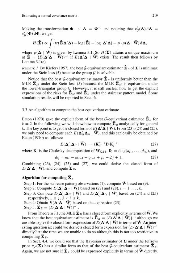
Making the transformation ��� → ��� = ���−1 and noticing that νlG(���) d��� =
where p(��� | W) is given by Lemma 3.1. So H(���) attains a unique maximumat ��� = {E(���′��� | W)}−1 if E(���′��� | W) exists. The result then follows byLemma 3.1(e).
Remark 1 By Kiefer (1957), the best G-equivariant estimator ���B of ��� is minimaxunder the Stein loss (5) because the group G is solvable.
Notice that the best G-equivariant estimator ���B is uniformly better than theMLE ���M under the Stein loss (5) because the MLE ���M is equivariant underthe lower-triangular group G. However, it is still unclear how to get the explicitexpressions of the risks for ���M and ���B under the staircase pattern model. Somesimulation results will be reported in Sect. 6.
3.3 An algorithm to compute the best equivariant estimate
Eaton (1970) gave the explicit form of the best G-equivariant estimator ���B fork = 2. In the following we will show how to compute ���B analytically for generalk. The key point is to get the closed form of E(���′��� | W). From (23), (24) and (25),we only need to compute each E(���′
ii���ii | W), and this can easily be obtained byEaton (1970) as follows:
E(���′ii���ii | W) = (K′
i )−1DiK−1
i (27)
where Ki is the Cholesky decomposition of Wi22·1, Di = diag(di1, . . . , dipi), and
dij = mk − mi−1 − qi−1 + pi − 2j + 1. (28)
Combining (23), (24), (25) and (27), we could derive the closed form ofE(���′��� | W), and compute ���B .
Algorithm for computing ���B
Step 1: For the staircase pattern observations (1), compute W based on (9).Step 2: Compute E(���′
ii���ii | W) based on (27) and (28), i = 1, . . . , k.Step 3: Compute E(���′
ij���ii | W) and E(���′ij���is | W) based on (24) and (25)
respectively, 1 ≤ j, s < i ≤ k.Step 4: Obtain E(���′��� | W) based on the expression (23).Step 5: ���B = {E(���′��� | W)}−1.
From Theorem 3.1, the MLE ���M has a closed form explicitly in terms of W. Weknow that the best equivariant estimator is ���B = {E(���′��� | W)}−1 although weare able to give the closed form expression of E(���′��� | W) in terms of W.An inter-esting question is: could we derive a closed form expression for {E(���′��� | W)}−1
directly? At the time we are unable to do so although this is not too restrictive incomputing ���B .
In Sect. 4.4, we could see that the Bayesian estimator of ��� under the Jeffreysprior πJ (���) has a similar form as that of the best G-equivariant estimator ���B .Again, we are not sure if ���J could be expressed explicitly in terms of W directly.
220 X. Sun and D. Sun
4 The Jeffreys and reference priors and posteriors
4.1 Bartlet decomposition
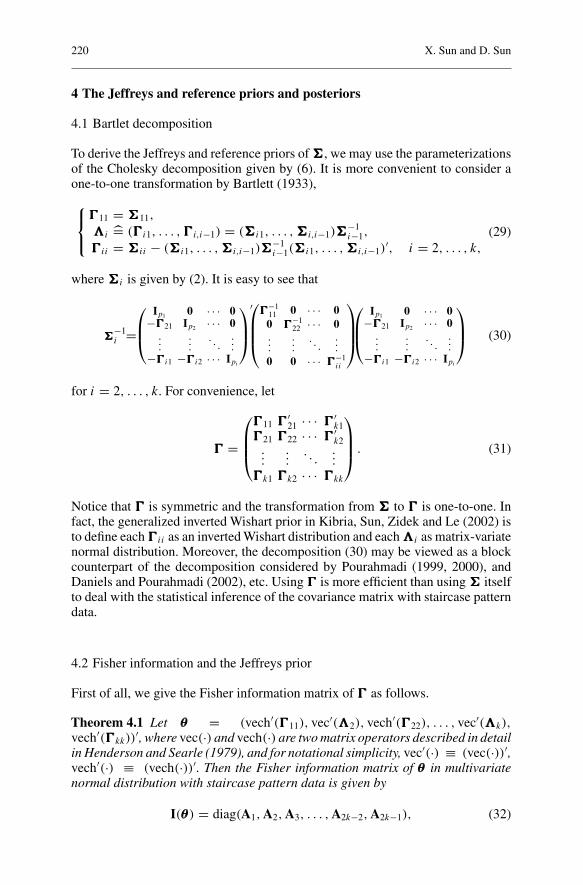
To derive the Jeffreys and reference priors of ���, we may use the parameterizationsof the Cholesky decomposition given by (6). It is more convenient to consider aone-to-one transformation by Bartlett (1933),
where ���i is given by (2). It is easy to see that
���−1i =
⎛
⎜⎝
Ip1 0 · · · 0−���21 Ip2 · · · 0
.
.
....
. . ....
−���i1 −���i2 · · · Ipi
⎞
⎟⎠
′⎛
⎜⎜⎝
���−111 0 · · · 00 ���−1
22 · · · 0...
.
.
.. . .
.
.
.
0 0 · · · ���−1ii
⎞
⎟⎟⎠
⎛
⎜⎝
Ip1 0 · · · 0−���21 Ip2 · · · 0
.
.
....
. . ....
−���i1 −���i2 · · · Ipi
⎞
⎟⎠ (30)
for i = 2, . . . , k. For convenience, let
��� =
⎛
⎜⎜⎝
���11 ���′21 · · · ���′
k1���21 ���22 · · · ���′
k2...
.... . .
...���k1 ���k2 · · · ���kk
⎞
⎟⎟⎠ . (31)
Notice that ��� is symmetric and the transformation from ��� to ��� is one-to-one. Infact, the generalized inverted Wishart prior in Kibria, Sun, Zidek and Le (2002) isto define each ���ii as an inverted Wishart distribution and each i as matrix-variatenormal distribution. Moreover, the decomposition (30) may be viewed as a blockcounterpart of the decomposition considered by Pourahmadi (1999, 2000), andDaniels and Pourahmadi (2002), etc. Using ��� is more efficient than using ��� itselfto deal with the statistical inference of the covariance matrix with staircase patterndata.
4.2 Fisher information and the Jeffreys prior
First of all, we give the Fisher information matrix of ��� as follows.
′, where vec(·) and vech(·) are two matrix operators described in detailin Henderson and Searle (1979), and for notational simplicity, vec′(·) ≡ (vec(·))′,vech′(·) ≡ (vech(·))′. Then the Fisher information matrix of θθθ in multivariatenormal distribution with staircase pattern data is given by
with Gi uniquely satisfying vec(���ii) = Gi · vech(���ii), i = 1, . . . , k.
The proof of the theorem is given in Appendix. We should point out that themethod in the proof also works for the usual complete data. We just need to replacemk − mi−1 by the sample size n of the complete data. Thus the Jeffreys prior forthe staircase pattern data will be the same as that for the complete data. The detailscan be seen in the following theorem.
Theorem 4.2 The Jeffreys prior of the covariance matrix ��� in multivariate normaldistribution with staircase pattern data is given by
πJ (���) ∝ |���|−(p+1)/2, (33)
which is the same as the usual Jeffreys prior for the complete data.
Proof It is well-known that for Ap×p and Bq×q , |A ⊗ B| = |A|q |B|p. Also, fromTheorem 3.13 (d) and Theorem 3.14(b) of Magnus and Neudecker (1999), it follows
|G′i (���
−1ii ⊗ ���−1
ii )Gi | = |G+i (���ii ⊗ ���ii)G+′
i |−1 = 2pi(pi−1)/2|���ii |−pi−1,
where G+i stands for the Moore–Penrose inverse matrix of Gi . Thus from (32), we
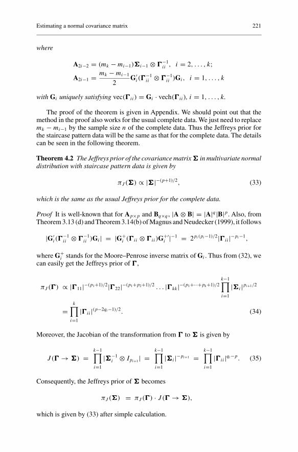
Moreover, the Jacobian of the transformation from ��� to ��� is given by
J (��� → ���) =k−1∏
i=1
|���−1i ⊗ Ipi+1 | =
k−1∏
i=1
|���i |−pi+1 =k−1∏
i=1
|���ii |qi−p. (35)
Consequently, the Jeffreys prior of ��� becomes
πJ (���) = πJ (���) · J (��� → ���),
which is given by (33) after simple calculation.
222 X. Sun and D. Sun
4.3 The reference prior
Suppose that each pi ≥ 2, i = 1, . . . , k. Because ���ii is still positive definite, itcan be decomposed as ���ii = O′
iDiOi , with Oi an orthogonal matrix with positiveelements for the first row and Di a diagonal matrix, Di = diag(di1, . . . , dipi
), withdi1 ≥ · · · ≥ dipi
, i = 1, . . . , k. With the similar idea in Yang and Berger (1994), areference prior may be derived in the following proposition.
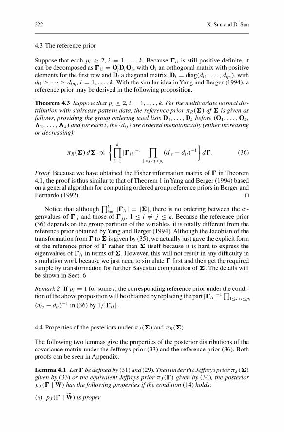
Theorem 4.3 Suppose that pi ≥ 2, i = 1, . . . , k. For the multivariate normal dis-tribution with staircase pattern data, the reference prior πR(���) of ��� is given asfollows, providing the group ordering used lists D1, . . . , Dk before (O1, . . . , Ok, 2, . . . , k) and for each i, the {dij } are ordered monotonically (either increasingor decreasing):
πR(���) d��� ∝{ k∏
i=1
|���ii |−1∏
1≤s<t≤pi
(dis − dit )−1
}
d���. (36)
Proof Because we have obtained the Fisher information matrix of ��� in Theorem4.1, the proof is thus similar to that of Theorem 1 in Yang and Berger (1994) basedon a general algorithm for computing ordered group reference priors in Berger andBernardo (1992). �
Notice that although∏k
i=1 |���ii | = |���|, there is no ordering between the ei-genvalues of ���ii and those of ���jj , 1 ≤ i �= j ≤ k. Because the reference prior(36) depends on the group partition of the variables, it is totally different from thereference prior obtained by Yang and Berger (1994). Although the Jacobian of thetransformation from ��� to ��� is given by (35), we actually just gave the explicit formof the reference prior of ��� rather than ��� itself because it is hard to express theeigenvalues of ���ii in terms of ���. However, this will not result in any difficulty insimulation work because we just need to simulate ��� first and then get the requiredsample by transformation for further Bayesian computation of ���. The details willbe shown in Sect. 6
Remark 2 If pi = 1 for some i, the corresponding reference prior under the condi-tion of the above proposition will be obtained by replacing the part |���ii |−1∏
1≤s<t≤pi
(dis − dit )−1 in (36) by 1/|���ii |.
4.4 Properties of the posteriors under πJ (���) and πR(���)
The following two lemmas give the properties of the posterior distributions of thecovariance matrix under the Jeffreys prior (33) and the reference prior (36). Bothproofs can be seen in Appendix.
Lemma 4.1 Let ��� be defined by (31) and (29). Then under the Jeffreys prior πJ (���)given by (33) or the equivalent Jeffreys prior πJ (���) given by (34), the posteriorpJ (��� | W) has the following properties if the condition (14) holds:
(a) pJ (��� | W) is proper
Estimating a normal covariance matrix 223
(b) ���11, ( 2, ���22), . . . , ( k, ���kk) are mutually independent(c) The marginal posterior of ���ii is IWpi
Here the definition of an IWp (inverse Wishart) distribution with dimension pfollows that on page 268 of Anderson (1984).
Lemma 4.2 Let ��� be defined by (31) and (29). Under the reference prior πR(���)given by (36), the posterior pR(��� | W) has the following properties if the condition(14) holds:
(a) pR(��� | W) is proper(b) ���11, ( 2, ���22), . . . , ( k, ���kk) are mutually independent(c) For i = 1, . . . , k,
pR(���ii | W) ∝ 1
|���ii |(mk−mi−1−qi−1)/2+1
×∏
1≤s<t≤pi
1
dis − dit
exp
{
−1
2tr(���−1
ii Wi22·1)}
;
(d) For i = 2, . . . , k, ( i | ���ii, W) ∼ Npi,qi−1(Wi21W−1i11, ���ii ⊗ W−1
i11);(e) The posterior mean of ���−1 is finite.
From Yang and Berger (1994), the Bayesian estimator of ��� under the Steinloss function (5) is ��� = {
E(���−1 | W)}−1
. So we have the following theoremimmediately.
Theorem 4.4 If the condition (14) holds, the Bayesian estimators of ��� underπJ (���) and πR(���) under the Stein loss function (5) uniquely exist.
Based on Lemma 4.1, an algorithm for computing Bayesian estimator ���J underπJ (���) can be proposed, which is similar to that for computing the best equivariantestimator ���B in Sect. 3.3. In Sect. 6, we will present an MCMC algorithm forcomputing Bayesian estimator ���R under πR(���).
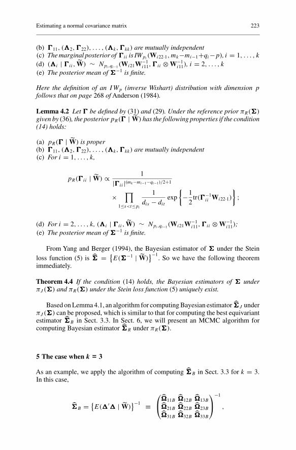
5 The case when k = 3
As an example, we apply the algorithm of computing ���B in Sect. 3.3 for k = 3.In this case,
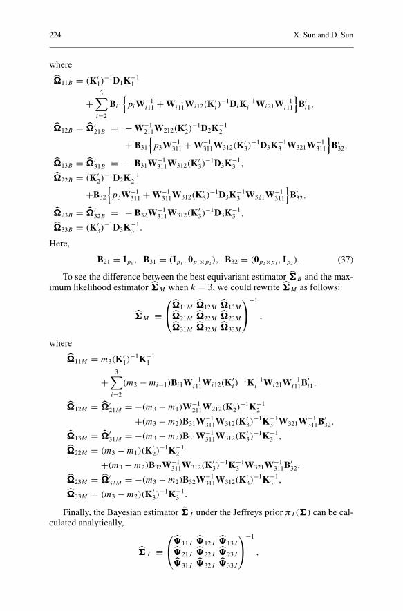
To see the difference between the best equivariant estimator ���B and the max-imum likelihood estimator ���M when k = 3, we could rewrite ���M as follows:
���M ≡⎛
⎝���11M ���12M ���13M
���21M ���22M ���23M
���31M ���32M ���33M
⎞
⎠
−1
,
where
���11M = m3(K′1)
−1K−11
+3∑
i=2
(m3 − mi−1)Bi1W−1i11Wi12(K′
i )−1K−1
i Wi21W−1i11B′
i1,
���12M = ���′21M = −(m3 − m1)W−1
211W212(K′2)
−1K−12
+(m3 − m2)B31W−1311W312(K′
3)−1K−1
3 W321W−1311B′
32,
���13M = ���′31M = −(m3 − m2)B31W−1
311W312(K′3)
−1K−13 ,
���22M = (m3 − m1)(K′2)
−1K−12
+(m3 − m2)B32W−1311W312(K′
3)−1K−1
3 W321W−1311B′
32,
���23M = ���′32M = −(m3 − m2)B32W−1
311W312(K′3)
−1K−13 ,
���33M = (m3 − m2)(K′3)
−1K−13 .
Finally, the Bayesian estimator ���J under the Jeffreys prior πJ (���) can be cal-culated analytically,
���J ≡⎛
⎝11J 12J 13J
21J 22J 23J
31J 32J 33J
⎞
⎠
−1
,
Estimating a normal covariance matrix 225
where
���11J = (m3 + p1 − p)W−1111 + p2W−1
211
+(m3 − m1 + p2 − p)W−1211W212W−1
222·1W221W−1211
+B31
{p3W−1
311 + (m3 − m2 + p3 − p)W−1311W312W−1
322·1W321W−1311
}B′
31,
���21J = ���′12J = (m3 − m1 + p2 − p)W−1
222·1W221W−1211
+B32
{p3W−1
311 + (m3 − m2 + p3 − p)W−1311W312W−1
322·1W321W−1311
}B′
31,
���31J = ���′13J = (m3 − m2 + p3 − p)W−1
322·1W321W−1311B′
31,
���32J = ���′23J = (m3 − m2 + p3 − p)W−1
322·1W321W−1311B′
32,
���22J = (m3 − m1 + p2 − p)W−1222·1
+B32
{p3W−1
311 + (m3 − m2 + p3 − p)W−1311W312W−1
322·1W321W−1311
}B′
32,
���33J = (m3 − m2 + p3 − p)W−1322·1.
Here B31 and B32 are given in (37).Unfortunately, it is almost impossible to calculate the Bayesian estimator ���R
analytically under the reference prior πR(���). Some simulation work will be givenin the next section.
6 Simulation studies
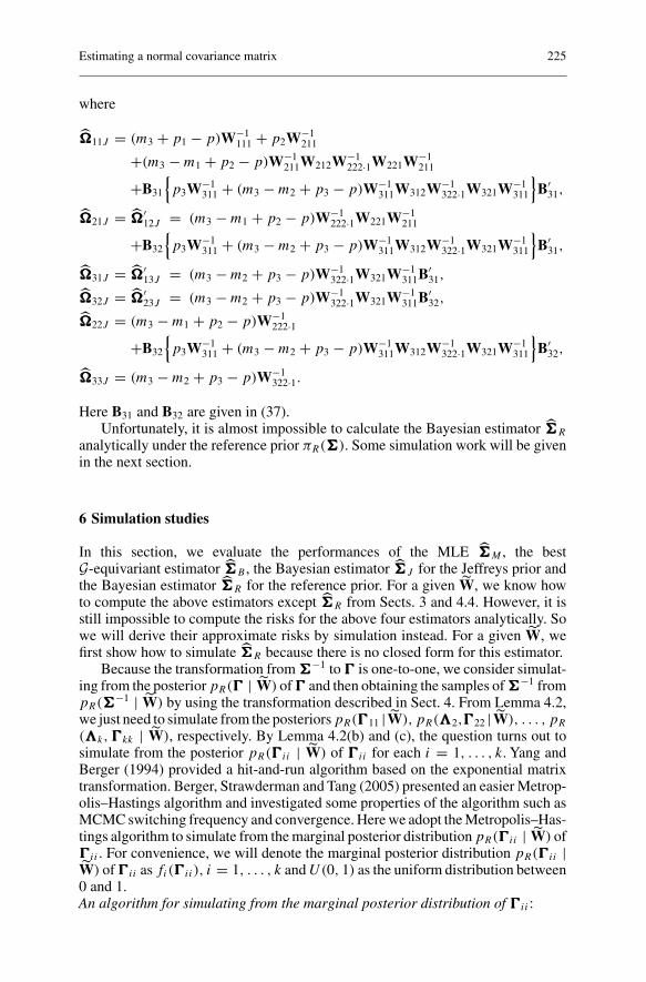
In this section, we evaluate the performances of the MLE ���M , the bestG-equivariant estimator ���B , the Bayesian estimator ���J for the Jeffreys prior andthe Bayesian estimator ���R for the reference prior. For a given W, we know howto compute the above estimators except ���R from Sects. 3 and 4.4. However, it isstill impossible to compute the risks for the above four estimators analytically. Sowe will derive their approximate risks by simulation instead. For a given W, wefirst show how to simulate ���R because there is no closed form for this estimator.
Because the transformation from ���−1 to ��� is one-to-one, we consider simulat-ing from the posterior pR(��� | W) of ��� and then obtaining the samples of ���−1 frompR(���−1 | W) by using the transformation described in Sect. 4. From Lemma 4.2,we just need to simulate from the posteriors pR(���11 |W), pR( 2,���22 |W), . . . , pR
( k, ���kk | W), respectively. By Lemma 4.2(b) and (c), the question turns out tosimulate from the posterior pR(���ii | W) of ���ii for each i = 1, . . . , k. Yang andBerger (1994) provided a hit-and-run algorithm based on the exponential matrixtransformation. Berger, Strawderman and Tang (2005) presented an easier Metrop-olis–Hastings algorithm and investigated some properties of the algorithm such asMCMC switching frequency and convergence. Here we adopt the Metropolis–Has-tings algorithm to simulate from the marginal posterior distribution pR(���ii | W) of���ii . For convenience, we will denote the marginal posterior distribution pR(���ii |W) of ���ii as fi(���ii), i = 1, . . . , k and U(0, 1) as the uniform distribution between0 and 1.An algorithm for simulating from the marginal posterior distribution of ���ii :
226 X. Sun and D. Sun
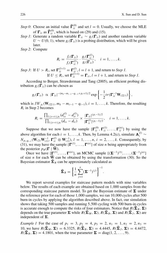
Step 0: Choose an initial value ���(0)ii and set l = 0. Usually, we choose the MLE
of ���ii as ���(0)ii , which is based on (29) and (15).
Step 1: Generate a random variable ���ii ∼ gi(���ii) and another random variableU ∼ U(0, 1), where gi(���ii) is a probing distribution, which will be givenlater.
Step 2: Compute
Ri = fi(���ii)
fi(���(l)ii )
· gi(���(l)ii )
gi(���ii), i = 1, . . . , k.
Step 3: If U > Ri , set ���(l+1)ii = ���
(l)ii , l = l + 1, and return to Step 1.
If U ≤ Ri , set ���(l+1)ii = ���ii , l = l + 1, and return to Step 1.
According to Berger, Strawderman and Tang (2005), an efficient probing dis-tribution gi(���ii) can be chosen as
gi(���ii) ∝ |���ii |−(mk−mi−1−qi−1+pi+1)/2 exp
{
−1
2tr(���−1
ii Wi22·1)}
,
which is IW pi(Wi22·1, mk − mi−1 − qi−1), i = 1, . . . , k. Therefore, the resulting
Ri in Step 2 becomes
Ri =∏
1≤s<t≤pi(d
(l)is − d
(l)it )
∏1≤s<t≤pi
(dis − dit )× |���ii |(pi−1)/2
|���(l)ii |(pi−1)/2
, i = 1, . . . , k.
Suppose that we now have the sample {���(0)ii , ���
(1)ii , . . . , ���
(n)ii } by using the
above algorithm for each i = 1, . . . , k. Then, by Lemma 4.2(c), simulate (l)i ∼
Npi,qi−1(Wi21W−1i11, ���
(l)ii ⊗ W−1
i11), l = 1, . . . , n, i = 2, . . . , k. Consequently, by(31), we may have the sample {���(1), . . . , ���(n)} of size n being appropriately fromthe posterior pR(��� | W).
Once we have {���(1), . . . , ���(n)}, an MCMC sample {(���−1)(1), . . . , (���−1)(n)}of size n for each W can be obtained by using the transformation (30). So theBayesian estimator ���R can be approximately calculated as
���R ={
1
n
n∑
j=1
(���−1)(j)
}−1
.
We report several examples for staircase pattern models with nine variablesbelow. The results of each example are obtained based on 1,000 samples from thecorresponding staircase pattern model. To get the Bayesian estimate of ��� underthe reference prior for each of those 1,000 samples, we ran 10,000 cycles after 500burn-in cycles by applying the algorithm described above. In fact, our simulationshows that taking 500 samples and running 5,500 cycling with 500 burn-in cyclesis accurate enough to compute the risks of four estimators. Notice that R(���R, ���)depends on the true parameter ��� while R(���M, ���), R(���B, ���) and R(���J , ���) areindependent of ���.
Example 1 For the case of p1 = 3, p2 = 4, p3 = 2, n1 = 1, n2 = 2, n3 =10, we have R(���M, ���) = 6.3325, R(���B, ���) = 4.4445, R(���J , ���) = 4.4472,R(���R, ���) = 4.1801, when the true parameter ��� = diag(1, 2, . . . , 9).
Estimating a normal covariance matrix 227
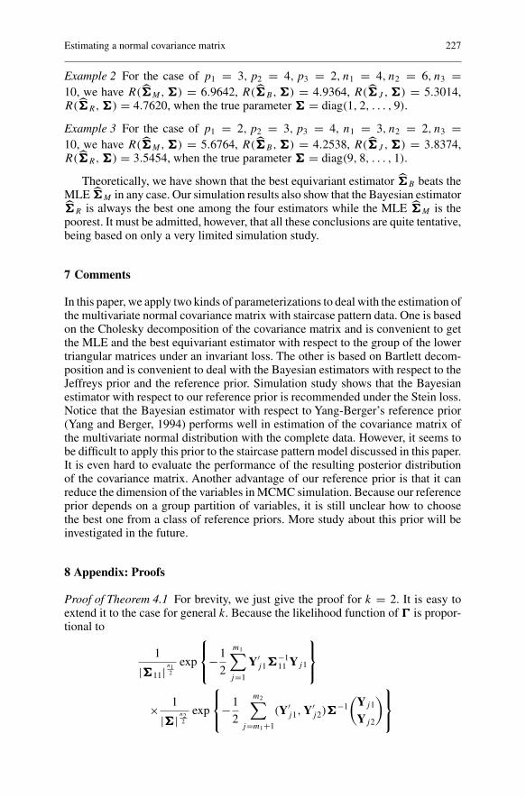
Example 2 For the case of p1 = 3, p2 = 4, p3 = 2, n1 = 4, n2 = 6, n3 =10, we have R(���M, ���) = 6.9642, R(���B, ���) = 4.9364, R(���J , ���) = 5.3014,R(���R, ���) = 4.7620, when the true parameter ��� = diag(1, 2, . . . , 9).
Example 3 For the case of p1 = 2, p2 = 3, p3 = 4, n1 = 3, n2 = 2, n3 =10, we have R(���M, ���) = 5.6764, R(���B, ���) = 4.2538, R(���J , ���) = 3.8374,R(���R, ���) = 3.5454, when the true parameter ��� = diag(9, 8, . . . , 1).
Theoretically, we have shown that the best equivariant estimator ���B beats theMLE ���M in any case. Our simulation results also show that the Bayesian estimator���R is always the best one among the four estimators while the MLE ���M is thepoorest. It must be admitted, however, that all these conclusions are quite tentative,being based on only a very limited simulation study.
7 Comments
In this paper, we apply two kinds of parameterizations to deal with the estimation ofthe multivariate normal covariance matrix with staircase pattern data. One is basedon the Cholesky decomposition of the covariance matrix and is convenient to getthe MLE and the best equivariant estimator with respect to the group of the lowertriangular matrices under an invariant loss. The other is based on Bartlett decom-position and is convenient to deal with the Bayesian estimators with respect to theJeffreys prior and the reference prior. Simulation study shows that the Bayesianestimator with respect to our reference prior is recommended under the Stein loss.Notice that the Bayesian estimator with respect to Yang-Berger’s reference prior(Yang and Berger, 1994) performs well in estimation of the covariance matrix ofthe multivariate normal distribution with the complete data. However, it seems tobe difficult to apply this prior to the staircase pattern model discussed in this paper.It is even hard to evaluate the performance of the resulting posterior distributionof the covariance matrix. Another advantage of our reference prior is that it canreduce the dimension of the variables in MCMC simulation. Because our referenceprior depends on a group partition of variables, it is still unclear how to choosethe best one from a class of reference priors. More study about this prior will beinvestigated in the future.
8 Appendix: Proofs
Proof of Theorem 4.1 For brevity, we just give the proof for k = 2. It is easy toextend it to the case for general k. Because the likelihood function of ��� is propor-tional to
1
|���11|n12
exp
⎧⎨
⎩−1
2
m1∑
j=1
Y′j1���
−111 Yj1
⎫⎬
⎭
× 1
|���| n22
exp
⎧⎨
⎩−1
2
m2∑
j=m1+1
(Y′j1, Y′
j2)���−1
(Yj1
Yj2
)⎫⎬
⎭
228 X. Sun and D. Sun
= 1
|���11|m22 |���22|
n22
exp
⎧⎨
⎩−1
2
m1∑
j=1
Y′j1���
−111 Yj1 − l∗
2
⎫⎬
⎭,
where
l∗ =m2∑
j=m1+1
(Y′j1, Y′
j2)
(Ip1 − ′
20 Ip2
)(���−1
11 00 ���−1
22
)(Ip1 0
− 2 Ip2
)(Yj1
Yj2
)
=m2∑
j=m1+1
(Y′j1, Y′
j2 − Y′j1
′2)
(���−1
11 00 ���−1
22
)(Yj1
Yj2 − 2Yj1
)
=m2∑
j=m1+1
Y′j1���
−111 Yj1 +
m2∑
j=m1+1
(Yj2 − 2Yj1)′���−1
22 (Yj2 − 2Yj1).
The log-likelihood becomes
log L = const − m2
2log |���11| − 1
2
m2∑
j=1
Y′j1���
−111 Yj1
−n2
2log |���22| − 1
2
m2∑
j=m1+1
(Yj2 − 2Yj1)′���−1
22 (Yj2 − 2Yj1).
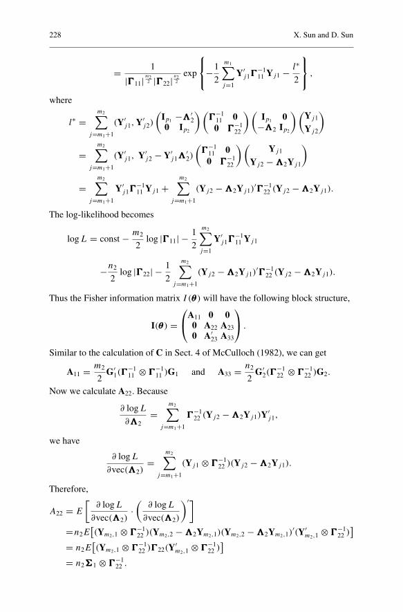
Thus the Fisher information matrix I (θθθ) will have the following block structure,
I(θθθ) =⎛
⎝A11 0 00 A22 A230 A′
23 A33
⎞
⎠ .
Similar to the calculation of C in Sect. 4 of McCulloch (1982), we can get
A11 = m2
2G′
1(���−111 ⊗ ���−1
11 )G1 and A33 = n2
2G′
2(���−122 ⊗ ���−1
22 )G2.
Now we calculate A22. Because
∂ log L
∂ 2=
m2∑
j=m1+1
���−122 (Yj2 − 2Yj1)Y′
j1,
we have
∂ log L
∂vec( 2)=
m2∑
j=m1+1
(Yj1 ⊗ ���−122 )(Yj2 − 2Yj1).
Therefore,
A22 = E
[∂ log L
∂vec( 2)·(
∂ log L
∂vec( 2)
)′]
=n2E[(Ym2,1 ⊗ ���−1
22 )(Ym2,2 − 2Ym2,1)(Ym2,2 − 2Ym2,1)′(Y′
m2,1 ⊗ ���−122 )]
= n2E[(Ym2,1 ⊗ ���−1
22 )���22(Y′m2,1 ⊗ ���−1
22 )]
= n2���1 ⊗ ���−122 .
Estimating a normal covariance matrix 229
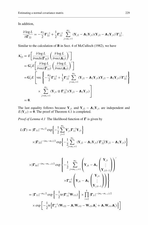
In addition,
∂ log L
∂���22= −n2
2���−1
22 + 1
2���−1
22
m2∑
j=m1+1
(Yj2 − 2Yj1)(Yj2 − 2Yj1)′���−1
22 .
Similar to the calculation of B in Sect. 4 of McCulloch (1982), we have
A′23 = E
[∂ log L
∂vech(���22)
(∂ log L
∂vec( 2)
)′ ]
= G′2E
[∂ log L
∂vec(���22)
(∂ log L
∂vec( 2)
)′ ]
=G′2E
⎡
⎣vec
⎧⎨
⎩−n2
2���−1
22 + 1
2���−1
22
m2∑
j=m1+1
(Yj2 − 2Yj1)(Yj2 − 2Yj1)′���−1
22
⎫⎬
⎭
×m2∑
j=m1+1
(Yj1 ⊗ ���−122 )(Yj2 − 2Yj1)
⎤
⎦
= 0.
The last equality follows because Yj1 and Yj2 − 2Yj1 are independent andE(Yj1) = 0. The proof of Theorem 4.1 is completed.
Proof of Lemma 4.1 The likelihood function of ��� is given by
L(���) = |���11|−mk/2 exp
{
−1
2
mk∑
j=1
Y′j1���
−111 Yj1
}
×|���22|−(mk−m1)/2 exp
{
−1
2
mk∑
j=m1+1
(Yj2 − 2Yj1)′���−1
22(Yj2 − 2Yj1)
}
×|���kk|−(mk−mk−1)/2 exp
⎧⎪⎨
⎪⎩−1
2
mk∑
j=mk−1+1
⎛
⎜⎝Yjk − k
⎛
⎜⎝
Yj1...
Yj,k−1
⎞
⎟⎠
⎞
⎟⎠
′
×���−1kk
⎛
⎜⎝Yjk − k
⎛
⎜⎝
Yj1...
Yj,k−1
⎞
⎟⎠
⎞
⎟⎠
⎫⎪⎬
⎪⎭
= |���11|−mk/2 exp
{
−1
2tr(���−1
11 W111)
}
×k∏
i=2
|���ii |−(mk−mi−1)/2
× exp
[
−1
2tr{���−1
ii (Wi22 − iWi12 − Wi21 ′i + iWi11
′i )}]
230 X. Sun and D. Sun
and thus the posterior of ���
pJ (��� | W) ∝ |���11|−(mk+2q1−p+1)/2 exp
{
−1
2tr(���−1
11 W111)
}
d���11
×k∏
i=2
|���ii |−(mk−mi−1+2qi−p+1)/2
× exp
[
−1
2tr{���−1
ii (Wi22 − iWi12 − Wi21 ′i + iWi11
′i )}]
=k∏
i=1
|���ii |−(mk−mi−1+qi+pi−p+1)/2 exp
{
−1
2tr(���−1
ii Wi22·1)}
×k∏
i=2
|���ii |−qi−1/2
× exp
[
−1
2tr{���−1
ii ( i − Wi21W−1i11)Wi11( i − Wi21W−1
i11)′}]
,
which shows the parts (b)(c) and (d). Here the condition (14) is required to guar-antee that Wi11, and Wi22·1 are positive definite with probability one for eachi = 1, . . . , k.
For (a), we know that pJ (��� | W) is proper if and only if pJ (���ii | W) is properfor each i = 1, . . . , k, and this is still guaranteed by the condition (14).
For (e), from (30), we get
���−1 =
⎛
⎜⎜⎝
Ip1 0 · · · 0−���21 Ip2 · · · 0
......
. . ....
−���k1 −���k2 · · · Ipk
⎞
⎟⎟⎠
′⎛
⎜⎜⎜⎝
���−111 0 · · · 00 ���−1
22 · · · 0...
.... . .
...
0 0 · · · ���−1kk
⎞
⎟⎟⎟⎠
⎛
⎜⎜⎝
Ip1 0 · · · 0−���21 Ip2 · · · 0
......
. . ....
−���k1 −���k2 · · · Ipk
⎞
⎟⎟⎠
=
⎛
⎜⎜⎝
11 12 · · · 1k
21 22 · · · 2k
......
. . ....
k1 k2 · · · kk
⎞
⎟⎟⎠ ,
where
ii = ���−1ii +
k∑
s=i+1
���′si���
−1ss ���si, i = 1, . . . , k − 1,
kk = ���−1kk ,
ij = ′ji = ���−1
ii ���ij +k∑
s=i+1
���′si���
−1ss ���sj , 1 ≤ j < i ≤ k − 1,
ki = ′ik = ���−1
kk ���ki, i = 1, . . . , k − 1.
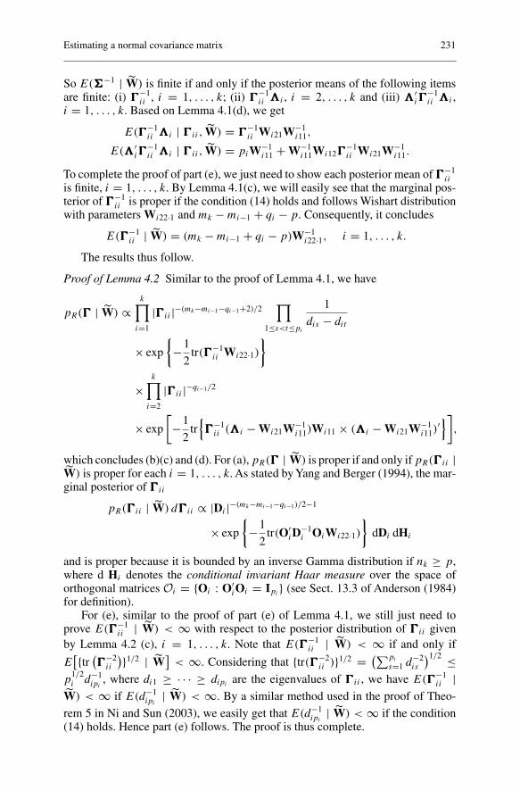
Estimating a normal covariance matrix 231
So E(���−1 | W) is finite if and only if the posterior means of the following itemsare finite: (i) ���−1
ii , i = 1, . . . , k; (ii) ���−1ii i , i = 2, . . . , k and (iii) ′
i���−1ii i ,
i = 1, . . . , k. Based on Lemma 4.1(d), we get
E(���−1ii i | ���ii, W) = ���−1
ii Wi21W−1i11,
E( ′i���
−1ii i | ���ii, W) = piW−1
i11 + W−1i11Wi12���
−1ii Wi21W−1
i11.
To complete the proof of part (e), we just need to show each posterior mean of ���−1ii
is finite, i = 1, . . . , k. By Lemma 4.1(c), we will easily see that the marginal pos-terior of ���−1
ii is proper if the condition (14) holds and follows Wishart distributionwith parameters Wi22·1 and mk − mi−1 + qi − p. Consequently, it concludes
E(���−1ii | W) = (mk − mi−1 + qi − p)W−1
i22·1, i = 1, . . . , k.
The results thus follow.
Proof of Lemma 4.2 Similar to the proof of Lemma 4.1, we have
pR(��� | W) ∝k∏
i=1
|���ii |−(mk−mi−1−qi−1+2)/2∏
1≤s<t≤pi
1
dis − dit
× exp
{
−1
2tr(���−1
ii Wi22·1)}
×k∏
i=2
|���ii |−qi−1/2
× exp
[
−1
2tr{���−1
ii ( i − Wi21W−1i11)Wi11 × ( i − Wi21W−1
i11)′}]
,
which concludes (b)(c) and (d). For (a), pR(��� | W) is proper if and only if pR(���ii |W) is proper for each i = 1, . . . , k. As stated by Yang and Berger (1994), the mar-ginal posterior of ���ii
pR(���ii | W) d���ii ∝ |Di |−(mk−mi−1−qi−1)/2−1
× exp
{
−1
2tr(O′
iD−1i OiWi22·1)
}
dDi dHi
and is proper because it is bounded by an inverse Gamma distribution if nk ≥ p,where d Hi denotes the conditional invariant Haar measure over the space oforthogonal matrices Oi = {Oi : O′
iOi = Ipi} (see Sect. 13.3 of Anderson (1984)
for definition).For (e), similar to the proof of part (e) of Lemma 4.1, we still just need to
prove E(���−1ii | W) < ∞ with respect to the posterior distribution of ���ii given
by Lemma 4.2 (c), i = 1, . . . , k. Note that E(���−1ii | W) < ∞ if and only if
E[{tr (���−2
ii
)}1/2 | W]
< ∞. Considering that {tr(���−2ii )}1/2 = (∑pi
s=1 d−2is
)1/2 ≤p
1/2i d−1
ipi, where di1 ≥ · · · ≥ dipi
are the eigenvalues of ���ii , we have E(���−1ii |
W) < ∞ if E(d−1ipi
| W) < ∞. By a similar method used in the proof of Theo-
rem 5 in Ni and Sun (2003), we easily get that E(d−1ipi
| W) < ∞ if the condition(14) holds. Hence part (e) follows. The proof is thus complete.
232 X. Sun and D. Sun
Acknowledgements The authors are grateful for the constructive comments from a referee. Theauthors would like to thank Dr. Karon F. Speckman for her carefully proof-reading this paper.The research was supported by National Science Foundation grant SES-0351523, and NationalInstitute of Health grant R01-CA100760.
References
Anderson, T. W. (1957). Maximum likelihood estimates for a multivariate normal distributionwhen some observations are missing. Journal of the American Statistical Association, 52,200–203.
Anderson, T. W. (1984). An introduction to multivariate statistical analysis. New York: Wiley.Anderson, T. W., Olkin, I. (1985). Maximum-likelihood estimation of the parameters of a multi-
variate normal distribution. Linear Algebra and its Applications, 70, 147–171.Bartlett, M. S. (1933). On the theory of statistical regression. Proceedings of the Royal Society
of Edinburgh, 53, 260–283.Berger, J. O., Bernardo, J. M. (1992). On the development of reference priors. Proceedings of
the Fourth Valencia International Meeting, Bayesian Statistics, 4, 35–49.Berger, J. O., Strawderman, W., Tang, D. (2005). Posterior propriety and admissibility of hyperp-
riors in normal hierarchical models. The Annals of Statistics, 33, 606–646.Brown, P. J., Le, N. D., Zidek, J. V. (1994). Inference for a covariance matrix. In: P. R. Freeman,
A. F. M. Smith, (Eds.), Aspects of uncertainty. A tribute to D. V. Lindley. New York: WileyDaniels, M. J., and Pourahmadi, M. (2002). Bayesian analysis of covariance matrices and dynamic
models for longitudinal data. Biometrika 89, 553–566.Dey, D. K., Srinivasan, C. (1985). Estimation of a covariance matrix under Stein’s loss. The
Annals of Statistics, 13, 1581–1591.Eaton, M. L. (1970). Some problems in covariance estimatio (preliminary report). Tech. Rep. 49,
Department of Statistics, Stanford University.Eaton, M. L. (1989). Group invariance applications in statistics. Hayward: Institute of Mathe-
matical Statistics.Gupta, A. K., Nagar, D. K. (2000). Matrix variate distributions. New York: Chapman & Hall.Haff, L. R. (1991). The variational form of certain Bayes estimators. The Annals of Statistics, 19,
1163–1190.Henderson, H. V., Searle, S. R. (1979). Vec and vech operators for matrices, with some uses in
Jacobians and multivariate statistics. The Canadian Journal of Statistics, 7, 65–81.Jinadasa, K. G., Tracy, D. S. (1992). Maximum likelihood estimation for multivariate normal dis-
tribution with monotone sample. Communications in Statistics, Part A – Theory and Methods,21, 41–50.
Kibria, B. M. G., Sun, L., Zidek, J. V., Le, N. D. (2002). Bayesian spatial prediction of randomspace-time fields with application to mapping PM2.5 exposure. Journal of the American Sta-tistical Association, 97, 112–124.
Kiefer, J. (1957). Invariance, minimax sequential estimation, and continuous time process. TheAnnals of Mathematical Statistics, 28, 573–601.
Konno, Y. (2001). Inadmissibility of the maximum likelihood estimator of normal covariancematrices with the lattice conditional independence. Journal of Multivariate Analysis, 79,33–51.
Little, R. J. A., Rubin, D. B. (1987). Statistical analysis with missing data. New York: Wiley.Liu, C. (1993). Bartlett’s decomposition of the posterior distribution of the covariance for normal
monotone ignorable missing data. Journal of Multivariate Analysis, 46, 198–206.Liu, C. (1999). Efficient ML estimation of the multivariate normal distribution from incomplete
data. Journal of Multivariate Analysis, 69, 206–217.Magnus, J. R., Neudecker, H. (1999). Matrix differential calculus with applications in statistics
and econometrics. New York: Wiley.McCulloch, C. E. (1982). Symmetric matrix derivatives with applications. Journal of the Amer-
ican Statistical Association, 77, 679–682.Ni, S., Sun, D. (2003). Noninformative priors and frequentist risks of bayesian estimators of
vector-autoregressive models. Journal of Econometrics, 115, 159–197.Pourahmadi, M. (1999). Joint mean-covariance models with applications to longitudinal data:
Pourahmadi, M. (2000). Maximum likelihood estimation of generalised linear models for mul-tivariate normal covariance matrix. Biometrika 87, 425–435.
Sun, D., Sun, X. (2005). Estimation of the multivariate normal precision and covariance matricesin a star-shape model. Annals of the Institute of Statistical Mathematics 57, 455–484.
Yang, R., Berger, J. O. (1994). Estimation of a covariance matrix using the reference prior. TheAnnals of Statistics, 22, 1195–1211.