Estimation of clinical dose distributions for breast and ... · Estimation of clinical dose...

Estimation of clinical dose distributions for breast and lung cancer radiotherapy treatments

Emma Hedin

Department of Radiation Physics

Institute of Clinical Sciences

Sahlgrenska Academy at University of Gothenburg

Gothenburg 2016

Cover illustration: Illustration of the fields in a stereotactic lung treatment (left)

and loco-regional breast treatment (right), prepared by Emma Hedin in the

Eclipse treatment planning system (Varian Medical Systems). Clinically used

plans applied on phantoms representing simplified human torsos.

Estimation of clinical dose distributions for breast and lung cancer

radiotherapy treatments

© Emma Hedin 2016

[email protected]

ISBN 978-91-628-9919-6 (PRINT)

ISBN 978-91-628-9920-2 (PDF)

E-publication: http://hdl.handle.net/2077/44924

Printed in Gothenburg, Sweden 2016

INEKO AB

http://hdl.handle.net/2077/44924

Finished.

Not Perfect.


Emma Hedin

Department of Radiation Physics, Institute of Clinical Sciences

Sahlgrenska Academy at University of Gothenburg

Göteborg, Sweden

ABSTRACT

The overall aim of this thesis was to investigate the uncertainties in the dose distribution

determined at the treatment planning stage. The work has been based on the main hypothesis

that the way of determining dose at the stage of treatment planning can be improved to such an

extent that it affects the risk-benefit assessment. Photon beam treatments of breast and lung

cancer were considered, i.e. treatments that are delivered to a region of the body that includes

lung tissue. Density inhomogenities are a challenge for the clinical dose calculation algorithms

(DCAs). Another challenge for the loco-regional breast cancer treatments are the adjacent fields

where the jaw positioning uncertainty may influence the uniformity of the dose distribution.

Different clinical DCAs were compared regarding their ability to calculate dose to lung (organ

at risk). The differences were quantified in terms of normal tissue complication probabilities

(NTCP) in Paper I. This study showed that the uncertainties in clinical DCAs can be of the same

magnitude as the uncertainties of published NTCP model parameters. Adjusted NTCP model

parameters were retrieved to avoid introduction of this additional uncertainty. The performance

of clinical DCAs regarding calculation of target dose for the case of stereotactic (small fields)

lung cancer treatments was compared to Monte Carlo (MC) calculations in Paper II. The

principle-based DCA Acuros XB (Varian, Eclipse) was found to comply better with MC than

the pencil-beam based analytical anisotropic algorithm (AAA) included in the study. The clinical

impact of the transition from the AAA to Acuros XB was discussed. In paper III and IV breast

cancer treatments were studied. The impact of jaw positioning uncertainty on the dose

distribution in the case of adjacent fields was investigated in paper III. The effect on lung tissue

was small whereas hotspots were found in soft tissue with unknown risks for plexus brachialis.

In paper IV the performance of different clinical dose calculation algorithms in lung tissue with

low density due to the breathing adaptive technique of deep inspiration breath hold (DIBH) was

investigated. The clinical impact of the transition from AAA to Acuros XB was discussed.

Acuros XB was compared to MC for the lowest lung density identified and the reliability of the

Acuros XB calculation was confirmed. The clinical impact of the transition from AAA to Acuros

XB was quantified for dose planning criteria based on different lung DVH parameters.

Keywords: External radiation therapy, breast cancer, lung cancer, clinical dose calculation

algorithms, Monte Carlo, NTCP, dose planning criteria

ISBN: 978-91-628-9919-6

POPULÄRVETENSKAPLIG SAMMANFATTNING PÅ SVENSKA

Strålterapi ges som behandling vid flera olika cancerdiagnoser.

Behandlingarna utformas för att maximera sannolikheten för tumörkontroll

och samtidigt minimera risken för biverkningar i normalvävnaden. Det är en

balansgång mellan risk-nytta som baseras på vetenskapliga studier och klinisk

erfarenhet av hur mycket stråldos som olika tumörer kräver samt hur mycket

stråldos som olika organ tål. Stråldosen beräknas av en dator när behandlingen

planeras. Risk-nytta bedömningen görs utifrån denna beräknade fördelning av

stråldosen i patienten. För att kunna göra en korrekt bedömning krävs korrekt

beräknade dosfördelningar. I denna avhandling studeras hur osäkerheterna ser

ut i de beräknade dosfördelningarna för bröst- och lungcancerbehandlingar. De

olika kliniska beräkningsmetoderna jämförs med en referensmetod som

innebär mycket noggrann och tidskrävande simulering av strålningens väg

genom patienten. Denna referensmetod kallas Monte Carlo-simulering.

Dessutom utreds hur dosfördelningen påverkas av osäkerheten i positionering

av de rörliga delarna i strålbehandlingsmaskinen. I vissa typer av

bröstcancerbehandlingar byggs dosfördelningen upp av två direkt anslutande

strålfält. Om dessa fält överlappar eller är separerade på grund av att en viss

inställning av fältets storlek inte efterlevs i verkligheten skulle potentiellt en

överdosering eller underdosering kunna ske i skarven.

Generellt visar resultaten att det finns osäkerheter i de beräknade

dosfördelningarna som är kliniskt relevanta. Den kliniska erfarenheten och de

vetenskapliga studierna baseras mest på dosfördelningar beräknade med tidiga

mindre exakta kliniska beräkningsmetoder. I utredningarna om

beräkningsmetoderna visades att risk-nytta bedömningar baserade på mer

nyligen introducerade kliniska beräkningsmetoder är potentiellt mer korrekta

men att justeringar bör göras av kriterierna som används vid planeringen av

behandlingen så att inte risk-nytta balansen oavsiktligt ändras. I studien om

närliggande fält och risken för att de överlappar eller är separerade framkom

att effekten på lungvävnad var liten men att det i fettvävnad och muskelvävnad

kan kvantifieras en överdosering, vilken kan medföra risker för nerver i

området.

i

LIST OF PAPERS

This thesis is based on the following studies, referred to in the text by their

Roman numerals.

I. Hedin, E. and Bäck, A. Influence of different dose

calculation algorithms on the estimate of NTCP for lung

complications. Journal of applied clinical medical physics

2013; 14(5):127–139.

II. Hedin, E., Chakarova, R. and Bäck, A. From AAA to Acuros

XB for lung cancer SBRT. Submitted

III. Hedin, E., Bäck, A. and Chakarova, R. Jaw position

uncertainty and adjacent fields in breast cancer

radiotherapy. Journal of applied clinical medical physics

2015; 16(6):240-251

IV. Hedin, E., Bäck, A. and Chakarova, R. From AAA to Acuros

XB for breast cancer treatment planning: Implications for

dose to lung tissue. Submitted

Appendix In the appendix a report concerning the development of the Monte Carlo model

is presented.

Hedin, E., Bäck, A., Swanpalmer, J. and Chakarova, R. Monte Carlo

simulation of linear accelerator Varian Clinac iX Report MFT-RADFYS

2010:01

ii

RELATED PUBLICATIONS

During my time as a PhD student I have contributed to two other published

studies.

Chakarova, R., Müntzing, K., Krantz, M., Hedin, E., and Hertzman, S.

Monte Carlo optimization of total body irradiation in a phantom and

patient geometry. Physics in Medicine and Biology 2013; 58(8):2461-9.,

Spang, F J., Rosenberg, I., Hedin, E. and Royle, G. Photon small-field

measurements with a CMOS active pixel sensor. Physics in Medicine and

Biology 2015; 60(11):4383-98.

iii

Preliminary results have been presented as follows

The effect of a change of dose calculation algorithm on NTCP for radiation

induced pneumonitis – A comparative study.

Emma Hedin, Roumiana Chakarova, Anna Bäck.

Poster at European Society for Radiotherapy & Oncology 29th conference

(ESTRO29). 2010, Barcelona, Spain.

Monte Carlo simulation of loco regional radiation treatment of breast

cancer: A case study.

Emma Hedin, Roumiana Chakarova, Anna Bäck

Poster at European Society for Radiotherapy & Oncology 31st conference

(ESTRO31). 2012, Barcelona, Spain.

Monte Carlo simulation of wedge fields: Implementing backscatter

correction.

Emma Hedin and Roumiana Chakarova

Oral presentation at SWE-RAYSs annual workshop. 2014, Malmö, Sweden.

Lung-DVHs from different algorithms

Emma Hedin, Anna Bäck and Roumiana Chakarova

Oral presentation at 3rd Öresund Workshop on Radiotherapy. 2015,

Helsingborg, Sweden.

From AAA to Acuros XB for lung SBRT

Emma Hedin, Roumiana Chakarova and Anna Bäck

Oral presentation at 4th Öresund Workshop on Radiotherapy. 2016,

Helsingborg, Sweden.

iv

CONTENT

ABBREVIATIONS ............................................................................................. VI

1 INTRODUCTION ........................................................................................... 1

2 AIM ............................................................................................................. 5

2.1 Paper I ................................................................................................... 5

2.2 Paper II .................................................................................................. 5

2.3 Paper III ................................................................................................ 6

2.4 Paper IV ................................................................................................ 6

3 THEORETICAL BACKGROUND ..................................................................... 7

3.1 Monte Carlo simulation with EGSnrc research code ............................ 7

3.1.1 Simulation of dynamic wedge ....................................................... 9

3.1.2 Impact of statistical noise on DVH ............................................. 11

3.2 Clinical dose calculation algorithms ................................................... 12

3.3 Uncertainties in jaw positioning ......................................................... 12

4 MATERIAL AND METHODS ........................................................................ 13

4.1 NTCP models ...................................................................................... 13

4.1.1 LKB-model.................................................................................. 13

4.1.2 RS-model ..................................................................................... 13

4.1.3 NTCP-model parameters from clinical studies ........................... 14

4.1.4 Method for adjusting model parameters ...................................... 15

4.2 Treatment planning ............................................................................. 16

4.2.1 Conventional lung treatments ...................................................... 16

4.2.2 Stereotactic lung treatments ........................................................ 16

4.2.3 Tangential breast cancer treatments ............................................ 17

4.2.4 Loco-regional breast cancer treatments ....................................... 17

4.3 Verification and implementation of the Monte Carlo model .............. 17

4.3.1 Absolute dose calibration ............................................................ 22

4.3.2 Backscatter correction ................................................................. 23

4.3.3 Backscatter correction for fields with wedge .............................. 24

v

4.3.4 Study-specific settings ................................................................. 25

4.4 Dose calculation with clinical dose calculation algorithms ................ 26

4.4.1 Study-specific settings ................................................................. 27

4.5 Study designs ...................................................................................... 28

5 RESULTS ................................................................................................... 31

6 DISCUSSION .............................................................................................. 41

7 CONCLUSIONS .......................................................................................... 45

7.1 Paper-specific conclusions .................................................................. 45

ACKNOWLEDGEMENT .................................................................................... 47

REFERENCES .................................................................................................. 48

APPENDIX ...................................................................................................... 53

vi

ABBREVIATIONS

3D / 4D Three/Four Dimensional

AAA Analytical Anisotropic Algorithm (DCA in Eclipse TPS)

AE Energy level above which secondary electrons are tracked

individually (secondary electrons with energy less than this

value are included in the CH)

AP Energy level above which secondary photons

(bremsstrahlung) are tracked individually (bremsstrahlung

photons with energy less than this are included in the CH)

AXB Acuros XB (DCA in Eclipse TPS)

BSCF Backscatter Correction factor

CC Collapsed Cone (DCA in Oncentra TPS)

CH Condensed History

CT Computed Tomography

CTV Clinical Target Volume

DCA Dose Calculation Algorithm

DIBH Deep Inspiration Breath Hold

DVH Dose Volume Histogram

ECUT Energy level below which the electron track is terminated and

all energy is deposited locally.

EDW Enhanced Dynamic Wedge

EUD Equivalent Uniform Dose

FB Free Breathing

GTV Gross Tumor Volume

ITV Internal Target Volume

LBTE Linear Boltzmann Transport Equation

LGL Loco-regional breast cancer treatment including

supraclavicular lymph nodes

LKB Lyman-Kutcher-Burman

MC Monte Carlo

vii

MLC Multi Leaf Collimator

MLD Mean Lung Dose

MU Monitor Unit (A certain amount of charge as measured by the

monitor chamber)

NTCP Normal Tissue Complication Probability

PB Pencil Beam (DCA in Oncentra TPS)

PBC Pencil Beam Convolution (DCA in Eclipse TPS)

PCUT Energy level below which the photon track is terminated and

all energy is deposited locally.

PTV Planning Target Volume

RS Relative-Seriality

SBRT Stereotactic Body Radiation Therapy

STT Segmented Treatment Table

Tang Tangential breast cancer treatment

TPS Treatment Planning System

V20Gy Parameter from the DVH. “The volume receiving the dose

20Gy or more”. The chosen dose level varies.

D98% Parameter from the DVH. “98% of the volume receives this

dose or more”. The chosen volume varies.

Emma Hedin

Introduction 1

1 INTRODUCTION

External radiation therapy is a commonly used treatment modality to treat

cancer either as a stand-alone treatment or in combination with surgery and/or

chemotherapy. Radiation dose in external radiation therapy is given to such a

level that the cancer cells are likely to be killed (high cure rate) but the function

of the normal tissue surrounding the cancer cells is likely to be maintained (low

risk for complication). This risk-benefit balance is assessed at the treatment

planning stage and impacts the design of the treatment plan. Today the risk-

benefit balance of a treatment is most often optimized based on the physical

dose distribution calculated in the treatment planning system (TPS), i.e. the

delivered dose distribution is estimated as equal to the dose as calculated in the

TPS. Unfortunately, the planned dose differ from the delivered dose

distribution for several reasons. This project focuses on uncertainties in the

calculation of dose at the planning stage that will affect the risk-benefit balance

assessment, i.e. differences that stem from approximations in the computer

algorithms for dose calculation and from technical tolerances of the positioning

of beam limiting collimators of the treatment machine.

There are other factors, not considered in this thesis, that may cause differences

between planned and delivered dose, for example, difficulties in reproducing

the patient geometry/position during planning and irradiation. The differences

emerge due to for example setup errors, breathing motions and tumor

shrinkage. Strategies to reduce those differences are, for example, breathing

adaptive techniques such as deep inspiration breath hold (DIBH) during

irradiation, on-board imaging to monitor tumor/patient position and different

patient fixation techniques. Nevertheless, since the current way of calculating

the risk-benefit balance is based on the optimum dose distribution as shown in

the TPS, the assessment of the risk-benefit balance made at the treatment

planning stage is unaffected by above mentioned factors.

In the clinical work flow the dose at the planning stage is calculated with dose

calculation algorithms (DCAs) in a TPS. In this thesis photon beam treatments

are considered. The DCAs include different methods for how to calculate dose

in the patient geometry. Today, this calculation is based on a CT scan or

magnetic resonance imaging scan of the patient. In this work CT scans are

considered. The calculation has to be relatively fast since the calculation is

performed several times per patient by the treatment planning staff while trying

to find a dose distribution that fulfills the treatment planning criteria. Since the

introduction of computer based dose calculations there has been a continuous

evolution of DCAs. The standard pencil beam convolution DCAs include pre-


2 Introduction

calculated pencil beam kernels and do not model changes in lateral electron

transport due to inhomogeneities. The DCA evolution then went via more

sophisticated algorithms with improved modelling of lateral electron scatter.

The most recent type of algorithm does not include pre-calculated scatter

kernels but are instead principle based algorithms using the principle of

simulating the radiation transport by tracking each individual particle or by

numerically solving the Linear Boltzmann Transport Equation (LBTE).

In this project breast and lung cancer treatments are investigated. Tangential

breast cancer treatments (Tang) with tangential fields covering the breast tissue

are studied as well as loco-regional breast cancer treatments (LGL) including

not only tangential fields but also anterior/posterior fields covering regional

(supraclavicular) lymph nodes. The lung cancer treatments studied are

conventional three-dimensional (3D) conformal treatments and stereotactic

body radiation therapy (SBRT) treatments. All those cancer treatments have in

common that they are delivered to a region of the body that includes lung

tissue. In other words, the tissue inhomogeneity is large in the CT scans that

the dose calculation is based on. For dose calculations in areas including lung

tissue, the approximations in the clinical DCAs may result in inaccurate dose

distributions [1], i.e. the dose is not accurately calculated in or near the lung

tissue. Hence, for both breast and lung cancer treatments, the dose to lung as a

risk organ is difficult to accurately assess as well as the dose to the target

volume, i.e. the volume required to have a certain dose coverage. For the breast

cancer treatments the target is in the vicinity of lung tissue and for the lung

cancer treatments the target may even consist partly of lung tissue. Another

challenge for the LGL case is the adjacent fields. The LGL plans investigated

in this work are constructed such that the anterior/posterior fields and the

tangential fields are matched in isocenter where there is no field divergence.

The matching of fields is a challenge since there are uncertainties in the jaw

positioning due to technical tolerances of the treatment machine. In the case of

adjacent fields the jaw positioning uncertainty becomes an issue since

overlapping fields may result in inadequate increase of dose and a gap between

fields in a region where homogeneous target dose is desired may result in

underdosage of target. Both the target coverage and dose to healthy tissue may

therefore be inaccurately estimated at the planning stage. In this work those

two factors, i.e. i) approximations in clinical DCAs and ii) impact of technical

tolerances on adjacent fields, are investigated regarding how they affect the

accuracy of dose calculation at the stage of treatment planning.

To make the work clinically relevant the inaccuracies in dose distributions are

quantified in terms of changes in the dose volume histograms (DVHs)

generally and also in terms of the dose volume histogram parameters

Emma Hedin

Introduction 3

commonly used in dose planning criteria, e.g. the target volume receiving at

least 100% of prescribed dose or the lung volume receiving more than 40% of

prescribed dose. In one of the studies in this work the differences in dose

distributions was quantified by differences in Normal Tissue Complication

Probability (NTCP) values for lung tissue.

As mentioned above, basing the risk-benefit balance assessment on the plain

physical dose rather than on an estimated biological effect in tissue is common

practice. One reason is that the uncertainties in the estimation of biological

effect are large. However, the transition from physical dose based evaluation

to evaluation based on estimates of biological effect has the potential of

improving clinical outcome since the biological effect is more correlated to

treatment outcome as compared to the plain physical dose. Ideally the

relationship between the delivered dose distribution and the risk for

complication would be known for each specific patient. As of today this is not

the case. The difficulties in determining the relationship between dose

distribution and probability of complication is an effect of many factors and

phenomena. For example, the average dose response curve must be modelled

for a certain population since the radiation sensitivity for each individual

patient is not known. The epidemiological studies therefore require large data

sets to reduce the statistical uncertainty to an acceptable level. Furthermore,

the determination of the delivered dose distribution, which is linked to the

response, is not trivial. The delivered dose distribution and the planned dose

distribution differ for several reasons as discussed above. In this work NTCP

models and published model parameters are used without any consideration of

their accuracy. However, the results of how the NTCP estimate is affected by

choice of algorithm also indicate how the uncertainties in the DCAs introduce

uncertainties in the NTCP modelling.

More accurate calculation of the dose distribution in or near lung tissue will be

of importance for both breast and lung cancer treatments. For conventional

lung cancer treatments lung toxicity in some cases limit how high dose that can

be delivered to the target. Therefore, a more accurate assessment of lung dose

is important to avoid delivering less dose than actually possible. Furthermore,

with a more reliable calculation the safety margins can be reduced. For lung

SBRT the dose is prescribed to a target partly consisting of lung tissue. Using

DCAs with approximate inhomogeneity corrections potentially results in

differences between prescribed/planned and delivered dose to target. The

breast cancer treatments are delivered to a large group of patients with a long

expected survival and in general in good health. This group will benefit from

more accurate calculation of lung dose and lung tissue NTCP estimates since


4 Introduction

this enables a reduction of the lung dose which can lead to a better quality of

life.

When evaluating clinical dose calculation algorithms the commonly used

reference method in the medical physics community is the Monte Carlo (MC)

method. Also in this work MC calculations are used for comparison to find and

quantify the weaknesses of the clinical DCAs. In general the MC calculations

involve simulation of individual particles transport trough the accelerator and

the patient. To distinguish between the clinical MC algorithms that involve

approximations to reduce calculation times the non-approximate MC method

is sometimes referred to as ‘full MC’. The full MC simulation is used as

reference method in this work. This method involves simulation of primary

particle transport through the treatment accelerator head for each field used

and then subsequent simulation of the particle transport within the

patient/phantom. The absolute dose calibration is based on measured data for

the calibration geometry. The MC method has the potential of being very

accurate. However, the accuracy depends on the input. For example, the

representation of the geometry of the accelerator head must be appropriate.

When measured and simulated data are found to comply for a number of fields

applied on a homogenous water phantom it is assumed that the systematic error

in simulated dose for any other geometry is small compared to the systematic

errors in the clinical DCAs. On the other hand, the MC method due to its nature

gives dose distributions with statistical noise. This must be recognized and

sufficient simulation time must be allowed to reduce the statistical noise so that

it does not have an impact on the result.

Emma Hedin

Aim 5

2 AIM

The studies in the current work are based on the main hypothesis that the way

of determining delivered dose at the stage of treatment planning can be

improved to such an extent that it affects the estimated risk of complication

and/or the appropriate treatment planning criteria.

2.1 Paper I

The objective of this work is to determine how to change the NTCP model

parameters for lung complications derived for a simple correction-based pencil

beam dose calculation algorithm in order to make them valid for other dose

calculation algorithms. The studied dose calculation algorithms are Pencil

Beam (PB) and Collapsed Cone (CC) both in Oncentra v4.0 TPS

(Nucletron/Elekta) as well as Pencil Beam Convolution (PBC) and Analytical

Anisotropic Algortihm (AAA) both in Eclipse v8.9 TPS (Varian Medical

Systems). This work includes three types of treatments — tangential and

locoregional breast treatment and conventional (no SBRT) lung treatment —

to study how the results are affected by the type of treatment. The effect on

NTCP of changing dose calculation algorithm is presented in relation to the

reported uncertainties in the original model parameters.

2.2 Paper II

The aim of this study is to quantify the individual differences between target

coverage calculated with two different DCAs and full MC respectively, for

SBRT lung treatment plans. The DCAs included in the study are AAA and

Acuros XB (AXB) in Eclipse v11.0.31 (Varian Medical Systems). SBRT plans

originally planned with AAA will be recalculated with AXB and MC and a

subgroup of plans presenting the largest differences between AAA and AXB

will be replanned with AXB to analyze the effect of changing from AAA to

AXB based treatment planning for SBRT lung treatments. The second aim is

to search for patient/plan characteristics that characterize the subgroup of plans

presenting larger differences between AAA and AXB. The overall goal is to

present complementary data needed for an attentive transition from AAA to

AXB for SBRT treatment planning.


6 Aim

2.3 Paper III

The objective of this work is to study the influence of the uncertainties in the

jaw position on the dose distribution in the patient geometry of a LGL

(including regional/supraclavicular lymph nodes) breast cancer treatment

which involves adjacent fields. Furthermore, it is investigated how a treatment

planning protocol including field overlap of 1 mm affects the situation. This

case study will contribute to the understanding of the benefits and disadvan-

tages of using 1 mm overlap and if there is a need for further optimization of

such a treatment protocol. The MC method is used to obtain the dose

distributions. It is a reference method for validation of clinical dose

calculations in the presence of heterogeneities, in the penumbra and in the

buildup region and allows for a 3D dose evaluation including the use of DVH

parameters currently used to specify dose planning criteria. The effect of ± 1

mm uncertainty in the jaw positioning is investigated by the two extreme

situations of gap and overlap of the adjacent fields that may happen in the

reality. In particular, these extremes are 2 mm gap or overlap in the case of a

planning protocol without gap or overlap, as well as 1mm gap and 3mm

overlap in the case of a planning protocol with 1 mm overlap (used in our

hospital for all loco-regional breast cancer treatments).

2.4 Paper IV

The overall goal of this study is to present data needed for the transition from

AAA to AXB by investigation of the differences in lung dose between AAA,

AXB and MC in free breathing (FB) CT-scans and DIBH (low lung density)

CT-scans, for both tangential and loco-regional (including

regional/supraclavicular lymph nodes) breast cancer treatment plans. The aim

is to describe the impact of lung density on the differences between AAA and

AXB by calculating two treatment plans per patient – one on FB CT scan and

one on DIBH CT scan. By evaluating the lung density in DIBH CT scans for

a large population the results are generalized. Furthermore, two cases of low

lung density are identified in this large population and calculated with AAA,

AXB as well as with full MC.

Emma Hedin

Theoretical background 7

3 THEORETICAL BACKGROUND

3.1 Monte Carlo simulation with EGSnrc research code

In the MC method the transportation of each particle in a radiation field is

simulated by sampling from probability distributions determining for example

type of interaction. With MC as reference dose calculation method the

calculation uncertainties due to model approximations are assumed to be small

compared to when TPS dose calculation algorithms are used. However, to

calculate a dose distribution with MC a model of the accelerator must be

accurately tuned by comparing MC calculated data with experimental data in

water phantom. Using the MC model for calculation of dose distributions in

patient geometry also requires an accurate representation of the patient

geometry with reliable tissue segmentation based on the CT image.

To ensure an accurate MC calculation there are also some basic underlying

information that must be accurate, including elemental material composition,

random number generators and probability distributions. In this

implementation of the MC method those factors are not assumed to be an issue

for the accuracy of the calculation.

There are different general MC transport codes. In this section the transport of

photons and electrons in EGSnrc will be briefly outlined. The general

procedure for photon MC simulation utilized in EGSnrc can be divided into

four steps (summary by Frederic Tessier presented on the IAEA course on the

EGSnrc code package, Trieste 2011. The details can be found in EGSnrc

documentation ‘PIRS-701’[2]).

1. Decide how far to go until next interaction

2. Transport on a straight line to the interaction site taking into

account geometry constraints.

3. Select which interaction takes place

4. Change energy and direction according to the corresponding

differential cross section.

When it comes to simulation of electron transport the approach is different.

Slowing down an electron results in many more interactions with surrounding

matter. Each interaction event therefore cannot be simulated separately due to

limitations in computer power. One solution to this is called ‘condensed

history’ (CH) technique and was developed by Berger et al. [3]. This technique


8 Theoretical background

is implemented in EGSnrc. In this technique all events where the energy loss

is smaller than a given value is ‘condensed’ and represented by one larger

electron step. The CH technique requires several algorithms and quantities to

accurately take all interactions into account. For example the concept of

restricted stopping power. The restricted stopping power is the total stopping

power excluding all events creating secondary particles with energy above the

energy level at which secondary particles are allowed. A secondary particle is

either an electron that is knocked out in an interaction event or a

bremsstrahlung photon. For electrons knocked out in an interaction event this

energy level is specified by the parameter AE and for bremsstrahlung photons

the corresponding parameter is AP. Details about restricted stopping power

and other essentials in the CH technique as implemented in EGSnrc can be

found in EGSnrc user’s manual PIRS-701 [2].

The user must also select the energy below which a particles track is terminated

and all energy is deposited locally. The parameter that sets this is called ECUT

for electrons and PCUT for photons.

The MC simulation of a treatment accelerator starts with electrons incident on

the target slab at the top of the accelerator head. Once the treatment head

geometry is defined according to specifications from the vendor the process of

adjusting the basic parameters for the model can start, i.e. the parameters

describing the characteristics of the electrons incident on the target slab. The

process is schematically described in Figure 1. It starts with a parameter guess

and then the particles exiting the accelerator head are collected collected in

BEAMnrc information about particle type, location, energy and direction is

stored in a ‘phase space’ file. The phase space is used as input in the next step

where dose is calculated in water phantom in DOSXYZnrc. Measured data and

simulated data are subsequently compared. The process is repeated until the

differences between measured data and simulated data are within acceptance

for all field sizes analyzed.

Emma Hedin


Schematic picture of the work of adjusting the basic parameters in the

MC model of the treatment accelerator head.

3.1.1 Simulation of dynamic wedge

To be able to deliver a desired dose distribution the accelerator head has

components that shapes the fields in a specific treatment. The collimator ‘jaws’

roughly limits the beam to the appropriate field size and the multi leaf

collimator (MLC) refines the shape of the field. Both are modelled in the MC

method. Furthermore, the treatments considered in this work sometimes

includes a dynamic wedge. For a field that includes a dynamic wedge one of

the jaws defining the field size in the y-direction is moving (closing the field)

during irradiation.

The MC method involves different techniques of sampling from probability

distributions using random numbers. To prepare for the work of simulating

dynamic wedges and the elaboration on backscatter (see section 4.3.4) the

sampling technique used for simulation of dynamic wedges in EGSnrc is

discussed briefly here.



Wedge fields are generated by the DYNJAWS[4, 5] code option following

Varian Enhanced Dynamic Wedge (EDW) implementation. The dynamic

movement of the upper jaws is controlled by the so-called segmented treatment

tables, STT. Each STT contains information on the jaw position versus dose

delivery information at different instances of the EDW field in form of

cumulative weighting of monitor units (MU). A single STT, (the one for 60°

wedge), is used to generate all the other STTs for various field sizes and wedge

angles.

By using this position probability sampling the movement of the jaw is

simulated to be continuous (more realistic) as opposed to the step and shoot

approximation.

Sampling from the cumulative probability distribution of a STT.

Transformation method! The dotted line is backscatter corrected, this is discussed

in Section 4.3.3

Why sampling from the cumulative probability distribution function is correct

can be intuitively understood. The random numbers are homogeneously

distributed between 0 and 1. We want a mapping that transforms this

homogeneously distributed variable to values of jaw position. The cumulative

probability distribution function is constructed such that when a random

number, say 0.45, is chosen on the y-axis (see Figure 2 above) this means that

45% of the random numbers are going to be below this value (since they are

homogeneously distributed) and also that 45% of the jaw position values are

going to be smaller than this value (according to the definition of the

cumulative probability distribution function). The jaw position values between

-20 and -15 in Figure 2 above will be more seldom chosen than jaw position

values between -5 and 0 since in the latter interval the STT curve is steeper.

The intervals can be made arbitrarily small and the reasoning is still valid.

Emma Hedin


3.1.2 Impact of statistical noise on DVH

Due to its nature the MC calculated dose distribution is fluctuating with

statistical noise. When the true dose distribution of a certain structure is

homogenous with all voxels in this structure receiving the same dose, then the

MC calculated dose distribution will have voxels appearing to receive both

smaller and larger dose than the true value. The impact of statistical noise in

the dose distribution on the DVH can be intuitively understood when this

homogeneous dose distribution is considered. The true DVH (cumulative) will

then consist of a horizontal line up until the dose value that all voxels receive

where the DVH abruptly decreases to zero. For the MC calculated dose

distributions some of the voxels receive smaller dose values than the true value.

Therefore, the MC calculated DVH curve will start to descend before the true

abrupt decrease of the DVH. Furthermore, the DVH will not decrease all the

way down to zero after the true dose value since some voxels are calculated to

receive a higher dose than the true value. So, the noise of the MC calculation

will cause the DVH to be flattened out, see an illustration of this in Figure 3.

The larger statistical uncertainties in the dose distributions the larger the effect

will be on the DVH. The dose distribution discussed so far is similar to that of

a target structure – similar dose to all voxels of the structure. For a risk organ

the dose distribution is much more inhomogeneous and the DVH will be

different. The same principle of how statistical noise (in the dose distribution)

affects the DVH of course also applies to the risk organs. However, for the risk

organs one also has to consider the situation of voxels with dose values close

to zero. A fairly large volume may receive low dose but in a noisy dose

distribution with few interactions only a fraction of this volume may be

‘detected’. Additionally, voxels with large relative statistical uncertainty

(small dose values and large statistical uncertainty) are commonly zeroed.

Illustration of how a true DVH is distorted by statistical noise in the MC

calculation.



3.2 Clinical dose calculation algorithms

In this work the clinical DCAs are used as ‘finished products’. There is no

attempt to suggest improvements or to explain the behavior of the algorithms

at any deeper knowledge level. Nevertheless, some basic information about the

algorithms has been helpful in formulation of research questions and is also

helpful in the discussion of the results.

The algorithms used are the Pencil Beam (PB) and Collapsed Cone (CC)

algorithms from Oncentra Masterplan TPS (Nucletron/Elekta) as well as Pencil

Beam Convolution (PBC) with modified Batho inhomogeneity correction,

Analytical Anisotropic Algortihm (AAA) and Acuros XB (AXB) from Eclipse

TPS (Varian Medical Systems). Different versions of the algorithms has been

used corresponding to the most recent version implemented at the hospital at

the time for the study.

The two standard pencil beam algorithms PB and PBC have different

approaches to for examples how to determine the pencil beam scatter kernels.

PB uses Monte Carlo calculated kernels whereas PBC uses a method based

only on the measured data described in [6]. How the scatter kernels are adjusted

in case of inhomogeneity in the patient/phantom are also different according

to the user manuals. They have that in common that the inhomogeneity

correction is only based on the density along the fan line, i.e. the

inhomogeneity correction does not include a correction of the lateral electron

scatter[1]. The DCA evolution then went via more sophisticated algorithms

such as AAA and CC. AAA include inhomogeneity correction of the scatter

kernels in multiple lateral directions (normal to the beam direction) [7], i.e. not

only in the beam direction which is the case in PB and PBC. CC is based on

point kernels[8] rather than pencil beam kernels that PB, PBC and AAA are

based on. The most recent type of algorithm used in this study is AXB. AXB

does not include pre-calculated scatter kernels but is instead principle based.

AXB numerically solves the Linear Boltzmann Transport Equation (LBTE)[9].

3.3 Uncertainties in jaw positioning

A method for determining the uncertainties in jaw positioning due to technical

tolerances has been developed earlier in our hospital [10]. It is based on EPID

(electronic portal imaging device) images of adjacent fields that are analyzed

for a particular gantry angle. Jaw positional uncertainty of up to 1 mm has been

detected for the Varian Clinac iX accelerators in our hospital and sometimes

systematic shifts that holds during an entire patient course.

Emma Hedin

Material and methods 13

4 MATERIAL AND METHODS

4.1 NTCP models

The normal tissue complication probability (NTCP) is used to evaluate the risk

for complication after radiotherapy. The NTCP value is calculated for a

specific end-point. For example, the end-points for lung tissue is commonly

different grades of pneumonitis.

Two NTCP models are used to calculate NTCP in this work. They are

described below. The lung DVHs are corrected for fractionation effects

according to the linear-quadratic model (LQ-model) using α/β = 3 Gy and dose

per fraction = 2 Gy. This is made to match the way the original model

parameters are retrieved.

4.1.1 LKB-model

NTCP is calculated using the Lyman-Kutcher-Burman model (LKB-model)

[11, 12] with the DVH reduced to EUD following Niemiero et al.[13] and

model parameters [D50, m, n]. The formula used for NTCP calculation

according to the LKB-model is described in Equation 1 and the formula for

calculating EUD for the NTCP model is described in Equation 2

dxeNTCP

t x

LKB

2

2

2

1

, (1)

where

50

50

mD

DEUDt

and

n

i

n

ii DEUD

/1 . (2)

4.1.2 RS-model

NTCP is also calculated using the Relative Seriality (RS)[14] model with the

model parameters [D50, γ, s]. The formula used for NTCP calculation

according to the RS-model is described in Equation 3, notation following

Rancati et al. [15] i is the fractional volume receiving the dose iD .


14 Material and methods

s

M

i

s

iRS

i

DPNTCP

/1

1

)(11

, (3)

where M is the number of subvolumes (number of dose bins in the DVH), and

)/1(exp( 502)(DDe

iiDP

.

For the LKB-model a reduction of the DVH to EUD is performed as a step in

calculating NTCP (see eq 2). To be able to plot NTCP values against a single

dose value, EUD is calculated also for the RS-model. For the RS-model EUD

is calculated from the NTCP value as the uniform dose that would yield the

same NTCP (see eq 4).

e

NTCPDEUDRS

*)2log(

)))log(log(1(*50

(4)

4.1.3 NTCP-model parameters from clinical studies

Model parameters were taken from four different studies [16-19]. The studies

are summarized in Table 1.

Table 1. Summary of the NTCP model parameter sets used.

Lung

volume

MLDa

Range

(Gy) Endpoint

Used on

treatment

type

Seppenwoolde et al. LKB paired

~2-35 RPc ≥ grade 2

SWOGd Lung, LGL,

Tang RS paired

Gagliardi et al. RS ipsilateral unknown RPc clinical LGL, Tang

Rancati et al. LKB ipsilateral

2.5-18

RPc ≥ grade 1

modified CTC-

NCICe LGL, Tang

RS ipsilateral

De Jaeger et al. b LKB paired ~2-25 RPc ≥ grade 2

SWOGd Lung

a Paired lungs b Parameters for the octree/edge algorithm with equivalent-pathlength inhomogeneity-correction c Radiation Pneumonitis d SouthWest Oncology Group toxicity criteria e Common Toxicity Criteria modified by the National Cancer Institute of Canada

Emma Hedin


4.1.4 Method for adjusting model parameters

The method used for adjusting model parameters for a different DCA than the

one used in the clinical study determining the model parameters is described

in detail in [20]. This method was implemented by the author of this thesis in

a MATLAB program. The concept of the method and the assumptions made

are briefly described here, following the notation in [20].

All parameters studied were retrieved for a standard pencil beam algorithm.

The aim was to find adjusted NTCP model parameters that in conjunction with

a given dose calculation algorithm would yield the same NTCP value that the

original parameters yield in conjunction with the standard pencil beam

algorithm. The tissue-describing parameters n and s were kept constant, while

D50 and m/γ were adjusted. The original model parameter set is denoted 𝑯0

and the parameter set to be used in conjunction with the new algorithms is

denoted 𝑯. The original NTCP value for the i:th patient is denoted

𝑃𝑁𝑇𝐶𝑃(𝑖, 𝑯0), this is calculated based on the standard pencil beam algorithm.

The NTCP value calculated based on the new algorithm is denoted

𝐶𝑁𝑇𝐶𝑃(𝑖, 𝑯). For a certain parameter set 𝑯𝒎𝒊𝒏 the difference between 𝑃𝑁𝑇𝐶𝑃

and 𝐶𝑁𝑇𝐶𝑃 is minimized. 𝑯𝒎𝒊𝒏 was found with a least-squares fitting

procedure. The 𝑃𝑁𝑇𝐶𝑃(𝑖, 𝑯0) and 𝐶𝑁𝑇𝐶𝑃(𝑖, 𝑯) were transformed by applying a

logarithm twice:

�̃�𝑁𝑇𝐶𝑃(𝑖, 𝑯0) = log (−log (𝑃𝑁𝑇𝐶𝑃))

�̃�𝑁𝑇𝐶𝑃(𝑖, 𝑯) = log (−log (𝐶𝑁𝑇𝐶𝑃))

The objective function to be minimized was as follows (the objective function

is denoted 𝜒2(𝑯) due to assumptions in the estimation of standard deviations

of adjusted parameters):

𝜒2(𝑯) = ∑[�̃�𝑁𝑇𝐶𝑃(𝑖, 𝑯0) − �̃�𝑁𝑇𝐶𝑃(𝑖, 𝑯)]2

�̃�𝑖2

𝑁

𝑖=1

where N is number of patients and �̃�𝑖 are the theoretical standard deviations

of the distribution of the difference �̃�𝑁𝑇𝐶𝑃(𝑖, 𝑯0) − �̃�𝑁𝑇𝐶𝑃(𝑖, 𝑯).

During the fitting process �̃�𝑖2 was set to unity. After the fit the standard

deviations of the adjusted parameters were estimated from the residuals of the

fit. The details of the equations can be found in [20]. The assumptions were:



- �̃�𝑖2 was assumed to be the same for each data point/patient

- the difference �̃�𝑁𝑇𝐶𝑃 - �̃�𝑁𝑇𝐶𝑃 was assumed to be normally

distributed. Normal probability plots were used to check

normality.

- The standard deviations of the parameter D50 was determined

by keeping m/γ constant at the value from the least-squares fit

and vice versa.

4.2 Treatment planning

The treatments in this study are all constructed according to current clinical

practice. Since only 3D conformal treatments are included in this work the only

time a beam limiting device is moving during irradiation is when dynamic

wedges are used. All plans are originally planned in the Eclipse TPS (Varian

medical systems) where the currently used dynamic wedges are called

enhanced dynamic wedge (EDW).

4.2.1 Conventional lung treatments

The exact field angles for the lung cases vary from case to case. They are based

on three beam directions — anterior, posterior, and from the ipsilateral side.

All lung plans use a photon energy of 6 MV for all fields. The beam directions

are optimized to restrict the dose to the spinal cord, the contralateral lung, and

the heart. Additional beams from the contralateral side are added if needed.

EDWs are used if needed. The prescribed dose is 35x2 Gy to the planning

target volume (PTV). PTV is defined as the clinical target volume (CTV) with

approximately 1 cm margin (depending on organ motion). CTV is defined as

the gross tumor volume (GTV) with 1 cm margin (or smaller if bone or air is

confining the volume).

4.2.2 Stereotactic lung treatments The treatment planning is done with 5-7 static coplanar or non-coplanar beams.

If a satisfactory dose distribution is obtained with a coplanar technique, this is

preferred to non-coplanar techniques. The beams are spread in the largest

possible angle. Opposed/overlapping beams on the skin is avoided. EDWs are

used if needed. Prescribed dose is 3x15 Gy minimum dose to the PTV,

centrally in PTV the dose can be up to 22 Gy per fraction. The PTV is defined

as the clinical target volume (CTV = the solid tumor and diffuse growth at its

borders) with a margin of 5 mm in transversal plane and 10 mm in the

longitudinal direction. In case of large tumor movement the margin is extended

to include all tumor positions by delineating CTV in all phases of a four-

dimensional (4D) CT (many 3D CT sets are obtained, each corresponding to a

Emma Hedin


particular breathing phase). An internal target volume (ITV) is then defined

which encompasses all the CTVs from the different 4D CT phases and PTV is

constructed by adding a margin to ITV. The stereotactic treatment is only given

to small tumors with maximal tumor diameter of 6 cm.

4.2.3 Tangential breast cancer treatments

The Tang plans include two main tangential 6MV photon beams toward the

breast. Additional small field segments of 6 or 15MV are sometimes used from

either direction to increase target-dose homogeneity. EDWs are used if needed,

but EDWs are not allowed if the treatment is delivered during DIBH. The

prescribed dose is 50 Gy. 95% of CTV should receive the prescribed dose and

the minimum dose to PTV must be larger than 93% (46.5 Gy). CTV consists

of the remaining breast tissue and PTV is defined as CTV with 5-10 mm

margin. PTV is also defined by the anatomy, for example the skin and lung

confines the extension of PTV.

4.2.4 Loco-regional breast cancer treatments

The LGL plans include 4-8 fields. Four main fields consisting of two tangential

fields towards the breast and additional two photon beams toward the axilla

region (anterior and posterior beams). Both 6 and 15 MV are used. The beam

arrangement is illustrated on the front cover (right figure). EDWs are used if

needed, but EDWs are not allowed if the treatment is delivered with gating.

The prescribed dose is 50 Gy, 95% of CTV should receive the prescribed dose

and the minimum dose to PTV must be larger than 93% (46.5Gy). CTV

consists of the remaining breast tissue. PTV is defined to include CTV with 5-

10 mm margin as well as the supraclavicular lymph nodes. PTV is also defined

by the anatomy, for example the skin and lung confines the extension of PTV.

4.3 Verification and implementation of the Monte Carlo model

The EGSnrc research code is in this work used by simulating the accelerator

head in BEAMnrc and then by simulating the transport of radiation in phantom

and in the patient geometry in DOSXYZnrc.

The virtual accelerator is defined by assorting certain modules predefined in

BEAMnrc. The modules, materials and dimensions are specified to resemble

the real accelerator as described in technical specifications released for

simulation purposes. A sketch of the 6 MV accelerator head simulated in this

work is shown in Figure 4.



Sketch of the virtual accelerator defined in BEAMnrc.

Emma Hedin


Both 6MV and 15MV photon fields are calculated. This requires two separate

MC models – one for the 6MV and one for the 15MV accelerator head. The

work of adjusting basic parameters for the 6MV accelerator head was made by

the author of this thesis and is reported in Appendix A (Report MFT-Radfys

2010:01). The Monte Carlo method was validated against measured data in

water phantom (profiles, depth dose curves and output factors) for an extensive

variety of field sizes (2x2 cm2 – 40x40 cm2). Model parameters for the 15 MV

accelerator head were adopted from [21, 22]. Additional work of validating the

model (6 and 15 MV) for mlc and wedge fields was made in paper III. Both

symmetric (not shown in Paper III) and asymmetric wedge fields were

validated against measurements. The mlc model was designed according to

technical specifications from the vendor and verified for static mlc fields (not

shown in Paper III). The measurements were conducted with an ion chamber

array (IC Profiler, Sun Nuclear Corporation).

Prior to using the MC model for a specific treatment type, example fields with

characteristics corresponding to the treatment type are applied on a water

phantom and calculated with the MC model and compared to measurement

and/or the clinical DCA. This is made to elucidate the accuracy of the model

in homogeneous geometry. The water phantom depth dose curve of a small

field of a stereotactic lung treatment as calculated by MC and clinical DCAs

as well as measured with a pin-point ionization chamber is shown in Figure 5.

The difference between the methods in dose maximum is up to 1.6 %. The

water phantom lateral profile for a double asymmetric rectangular field

including wedge (15 degrees) is shown in Figure 6, the MC calculation is

compared to a relative measurement with ion chamber array (IC Profiler, Sun

Nuclear Corporation, 251 ion chambers with 2.9 mm width and 5 mm spacing)

as well as absolute measurement with ionization chamber CC13 (IBA

Dosimetry, Germany).



Water phantom depth dose curve of 3x3 cm3 field. Calculated with MC

model, AAA and AXB as well as measured with pin-point ionization chamber.

Water phantom lateral profile for tangential field in LGL breast

treatment. 15 degree wedge, double asymmetric. MC calculation (solid black line)

compared with ion chamber array measurement (grey dots) which is a relative

measurement normalized to the absolute ion chamber measurement (cross).

Emma Hedin


The model transport parameters used during calculation of clinical treatment

plans are shown in Figure 7-8.

EGSnrc transport parameters used in the BEAMnrc simulations.

EGSnrc transport parameters used in the DOSXYZnrc simulations.



For the BEAMnrc simulations (phase space collection) AE was chosen to be

0.700MeV with ECUT=AE and AP was chosen to be 0.01MeV with

PCUT=AP. For the DOSXYZnrc simulations (dose calculation) AE was

chosen to be 0.521 MeV with ECUT=AE and AP was chosen to be 0.01 MeV

with PCUT=AP. This is following the recommendations for therapy beam dose

calculations in the BEAMnrc user’s manual [4] and is coherent with or more

detailed than other published similar work [23-26].

The settings above implies that electrons in the phantom/patient are followed

down to total energy of 0.521MeV. According to recommendations in

BEAMnrc user’s manual [4] “ECUT should be chosen so that the electron’s

range at ECUT is less than about 1/3 of the smallest dimension in a dose

scoring region”. To follow this recommendation the density in the CT image

or the voxel dimensions of the calculation must be kept above certain values.

For example for the MC model to accurately simulate the dose distribution in

air (0.001205g/cm3) the smallest voxel dimension allowed is 7 mm. For a 2

mm voxel dimension (common clinical dose grid) the lowest density

accurately simulated is 0.0038 g/cm3 (using the CSDA range for water).

Probability distributions for the chosen AE and AP are constructed in the

PEGS software included in the EGSnrc code package. Nine tissue types are

defined, namely; air, lung, adipose, muscle skeletal and five bone tissues

obtained by interpolation of bone mass density and composition between

spongiosa skeletal and cortical bone. The elemental composition of the

materials included are calculated according to the formalism in [27] and [28].

4.3.1 Absolute dose calibration

The formalism for conversion of the MC dose in Gy per primary history to the

dose in Gy for a certain number of monitor units MU (denoted further in the

text as absolute dose) is based on simulations of the calibration geometry and

corrections for the effect of backscattered radiation to the monitor chamber, as

described in [29]. The accelerators in our hospital are calibrated in water at 10

cm depth at source-to-surface distance (SSD) 90 cm for a 10 cm × 10 cm field.

The MC model is solely used to report dose to medium, no conversion to dose

to water is made.

This empirical approach for absolute calibration is commonly used in the

context of Monte Carlo calculation of radiation therapy beams. The relative

dose (normalized to number of primary particles) from the MC simulations is

related to the relative dose in the calibration point. Furthermore, the number of

MUs for each field is related to the number of MUs per Gy in the calibration

Emma Hedin


point. However, the MUs are measured with the monitor chamber that is placed

above the jaws and therefore a small fraction of the signal from the monitor

chamber is from radiation that has interacted in the jaws and are backscattered

towards the monitor chamber. The amount of backscattered radiation to the

monitor chamber varies with field size since the larger fields the smaller parts

of the jaws are in the field. The monitor chamber response is not modelled in

the MC simulation and therefore the backscatter must be corrected for without

knowing the actual amount of charge in the monitor chamber produced by

backscattered radiation. For small fields the charge representing one MU is

reached faster than expected. This means in turn that 1 MU is not ‘worth’ as

much dose below the accelerator head as expected. The ratio between the

measured absolute dose and the simulated absolute dose (not backscatter

corrected) for this small field size gives us a clue about how the number of

MUs for a given field should be adjusted to correspond to the number of MUs

measured with a monitor chamber not subject to backscattered radiation at all,

i.e. the number of MUs suitable for input to the MC model. The backscatter

correction is further discussed below.

4.3.2 Backscatter correction

A backscatter correction factor (BSCF) is used that relates the amount of

backscattered dose to the monitor chamber for a certain field to the calibration

field size. A linear dependence is considered between the backscattered dose

to the monitor chamber and the field size as suggested by Verhaegen et al.[30]

It is assumed that the effect of the components located below the upper Y jaw,

namely the lower X jaw and the MLC, is negligible. This assumption is

consistent with the results reported on the dominating effect of the upper Y jaw

on the backscatter compared to that of the lower X jaw.[30, 31] The BSCF is

therefore only dependent on the field length in the Y direction (FSy) and is

given by:

𝐵𝑆𝐶𝐹(𝐹𝑆𝑦) =𝑎+𝑏∗10

𝑎+𝑏∗𝐹𝑆𝑦 (1)

New parameter values of 𝑎 and 𝑏 in Equation 1, specific for our accelerators,

are obtained, namely, a = 1.034 (1.028) and b = -0.00085 (-0.00070) for 6 (15)

MV, respectively. The field sizes included in this optimization procedure are

4x4 cm, 20x20 cm and 40x40 cm symmetrical square fields, as well as 4x20

cm and 20x4 cm symmetrical rectangular fields. The process of retrieving the

parameters including minimizing the difference between simulated and

measured output factors.



This method of correcting for backscatter is experimental and is not based on

any simulation of the monitor chamber. As shown in Figure 9 after backscatter

correction the difference between measured and simulated output factors is less

than 1% for the 6MV accelerator head model and less than 0.5% for the 15 MV

accelerator head, for the investigated field sizes.

Differences between MC-calculated and measured output factors for

both non-corrected MC-calculated values (gray) and backscatter corrected MC-

calculated values (white).

4.3.3 Backscatter correction for fields with wedge

For wedges, the backscatter correction is applied on the differential segmented

treatment table; STTdiff,i = STTi – STTi-1, where i is an index indicating the

row of the STT. To facilitate the writing in Equation 2, it is defined

that 𝑆𝑇𝑇 0 = 0. The row-index, i , varies from 1 to maximum number of rows

in the STT. Each row of the backscatter corrected STT, 𝑆𝑇𝑇𝑏𝑠𝑐𝑜𝑟𝑟, is thereby

given by:

𝑆𝑇𝑇𝑏𝑠𝑐𝑜𝑟𝑟,𝑖 = ∑ ((𝑆𝑇𝑇 𝑖 − 𝑆𝑇𝑇 𝑖−1) ∗ 𝐵𝑆𝐶𝐹(𝐹𝑆𝑦𝑖))𝑖1 (2)

In this way, the backscatter effect is taken into account when simulating the

jaw movement. The backscatter corrected STT is normalized to the number of

cumulative monitor units, delivered at the last position of the jaw, before it is

used in the EGSnrc/BEAMnrc for producing a phase space. The number of

MUs of a wedged field is in the treatment plan equal to the cumulative number

of MUs delivered at the last position of the jaw. Therefore, a backscatter

correction factor, (denoted global in the text), is needed also for wedged fields

- so that the total number of MUs can be corrected in a similar way as for to

Emma Hedin


the non-wedge fields. This global backscatter correction factor used for wedge

fields in the conversion of the MC dose to absolute dose is obtained by the ratio

between the cumulative number of MUs for backscatter corrected and non-

corrected STT, respectively. A backscatter corrected STT is compared to the

original STT in Figure 2 in Section 3.1.1.

4.3.4 Study-specific settings

The MC model is used in three out of four papers to recalculated treatment

plans originally planned with one of the clinical DCAs. During recalculation

the same number of monitor units, MLC/collimator positions, EDWs and beam

arrangement are used as in the original plan. The number of histories required

in the MC calculations to achieve acceptable statistical noise was determined

by test calculations for each treatment type. The number of histories was

increased until there was no visual effect on the DVH.

Paper II In this study the MC calculation was made with dose scoring in cubical voxels

with 2 mm sides. The results are compared to the AXB algorithm. In the AXB

algorithm materials are mixed when the mass density is in a certain interval,

i.e. the border between for instance lung/adipose tissues is not sharp but in a

given mass density interval both lung and adipose tissue are present. For MC

simulations a distinct border between different tissue types is used. To match

the AXB calculations as good as possible, this border was chosen at the mean

of the mass density interval used for mixed materials in AXB. The 3D dose

distributions are analyzed in CERR (Matlab based computational environment

for radiotherapy research).

Paper III In this paper the MC model is used to investigate jaw misalignment of up to a

few millimeters. Therefore, the resolution is improved compared to normal

clinical dose grids and the MC calculation is made with dose scoring in cubical

voxels with 1.5 mm sides. Nine tissues are defined in the tissue segmentation

process, similar to how it is done in Paper II. However, the MC results are not

explicitly compared to a clinical DCA in this study why the tissue types are not

chosen according to the tissue segmentation table from AXB (as in Paper II

and IV). Instead, the density intervals for each material are somewhat

arbitrarily chosen, but they are defined to match with the tissue inserts used

during CT calibration. The densities are also compared to the material density

of each tissue type as reported in ICRU Report 44 [32]. The 3D dose

distributions are imported as DICOM dose files via Vega library[33] in the

Eclipse v. 11.0 (Varian Medical Systems) TPS for viewing and DVH analysis.



Paper IV In this paper the MC calculations were made with dose scoring in voxels with

dimension of 2 mm in the transversal plane and 3 mm between CT-slices. In

this study breast treatment plans are applied on patient CT scans with low lung

densitiy due to DIBH gating technique. For the two low-density cases

identified, the amount of voxels with density less than 0.0041 g/cm3 in the lung

tissue was quantified. Below this density the 2 mm voxel dimension is too

small for the chosen ECUT as recommended by Walters et al. [4]. The tissue

segmentation is in this study identical to Paper II since MC is compared to

AXB. The 3D dose distributions are analyzed in CERR (Matlab based

computational environment for radiotherapy research).

4.4 Dose calculation with clinical dose calculation algorithms

The configuration of the DCAs are identical to the clinical implementation.

The physical material table used for all AXB calculations are presented in

Table 2.

Table 2. Physical material table used in the AXB calculations

Material name Minimum

Density (g/cm3)

Maxium Density

(g/cm3)

Air 0.0000 0.0204

Lung 0.0110 0.6242

Adipose 0.5539 1.0010

Muscle 0.9693 1.0931

Cartilage 1.0556 1.6000

Bone 1.1000 3.000

Emma Hedin


4.4.1 Study-specific settings

Paper I In paper I the studied dose calculation algorithms are Pencil Beam (PB) and

Collapsed Cone (CC) both in Oncentra v4.0 TPS (Nucletron/Elekta) as well as

Pencil Beam Convolution (PBC) with modified Batho inhomogeneity

correction and Analytical Anisotropic Algortihm (AAA) both in Eclipse v8.9

TPS (Varian Medical Systems). The calculation grid is 2.5 mm with a 5 mm

slice separation of the CT series. The plans are originally calculated with PBC.

The plans are recalculated with AAA and also exported to Oncentra where they

are recalculated with PB and CC. The MUs obtained in the PBC calculation

are used in all recalculations.

Paper II The original treatment plans were planned based on AAA in Eclipse (version

11.0.31, Varian Medical Systems). All plans were recalculated with AXB

(Eclipse, version 11.0.31). The same number of MUs, MLC/collimator

positions, EDWs and beam arrangement were used for the recalculated

treatment plans. A clinically realistic dose grid of 2 mm was used for all dose

calculations, including 2 mm slice separation of the CT series.

Paper III Test calculations are performed with the dose calculation algorithm currently

used at our hospital for this type of treatment, namely the analytical anisotropic

algorithm (AAA) version 10.0.28 implemented in Eclipse (Varian Medical

Systems). A dose grid of 1.5 mm is used since the investigated issue involves

misalignment of jaws of a few millimeters.

Paper IV All treatment plans were originally planned with AAA and they were

recalculated with AXB using the same number of MUs, MLC/collimator

positions, EDWs and beam arrangement. A clinically realistic dose grid of 2

mm in the transversal plane and 3 mm between CT-slices were used for all

dose calculations. Throughout the study AAA and AXB version 13.6.23 was

used.



4.5 Study designs

Paper I 10 tangential breast (Tang), 10 loco-regional breast (LGL) and 10 lung cancer

treatment plans are included in the study (see detailed description of the types

of treatments in section 3.3). The plans are originally calculated with PBC in

Eclipse. The plans are recalculated with AAA and also exported to Oncentra

where they are recalculated with PB and CC. The MUs obtained in the PBC

calculation are used in all recalculations. Lung DVHs are compiled in their

respective TPS and used to estimate NTCP. GTV is subtracted from the lung

DVH in the case of lung cancer. The DVHs are retrieved for paired lungs and

in the case of breast cancer treatment also for the ipsilateral lung.

The mean lung dose (MLD), NTCP and equivalent uniform dose (EUD) are

calculated for all DVHs and for all four calculation algorithms. NTCP is

calculated using the LKB-model[11, 12] with the DVH reduces to EUD,

following Niemerko[13] and the relative seriality (RS) model[14]. The model

parameters derived for a correction-based pencil beam dose calculation

algorithm are taken from four different publications describing studies that

consider different grades of pneumonitis.

The original parameters were assumed to be valid for PB. The impact of choice

of DCA on the NTCP values is illustrated by plotting the reference NTCP value

against its different EUDs as calculated by the different DCAs. Furthermore,

new NTCP model parameters for PBC, AAA, and CC were derived following

the method suggested by Brink et al. [20], this method is discussed in section

3.2.1. The impact of choice of DCA on the NTCP is also compared to the

statistical uncertainties in the model parameters as reported from the clinical

trials.

Paper II 20 SBRT lung treatments (detailed description of the treatment type in section

3.3) are included in the study. The original treatment plans were based on AAA

and were recalculated with AXB as well as with full MC. The MUs obtained

in the AAA calculation were used in all recalculations.

The dose calculation methods were compared for all treatment plans by visual

analysis of total DVHs for GTV and PTV and the differences were quantified

by D5%, D50% and D98%. PTV-V100% was also retrieved to investigate the

feasibility of a 100% isodose prescription to PTV.

Emma Hedin


For each case the patient/plan characteristics listed below were recorded.

Those plan/patient characteristics were recorded to investigate if they can be

used to predict the change in calculated target dose coverage when changing

dose calculation method from AAA to AXB.

- GTV volume

- PTV volume

- Volume of lung tissue part of PTV

- Distance from GTV edge to nearest lung edge

- Average of lung density in three points two centimeters from

PTV

- Proportion of PTV edge in lung.

For the plans with largest change in PTV-V100%, when the plan was

recalculated with AXB, a re-planning was made based on AXB’s dose

calculation. During re-planning with AXB, PTV-V100% was kept within 0.5%

of the value of the original AAA plan. The treatment planning criteria for this

treatment type are described in section 3.3, for the re-planned cases additional

parameters were recorder apart from what is determined in the treatment

planning criteria, namely mean dose to GTV and volume encompassed by the

100% isodose.

Paper III In this paper one LGL breast treatment is considered. Dose distributions are

obtained for the following five cases of junction between the cranial fields and

the tangential fields: 2 and 1 mm gap, perfect match, as well as 2 and 3 mm

overlap.

DVH parameters are evaluated for PTV, Body and Body minus PTV. V105%,

V110% and V120% are chosen to illustrate the increased volumes of hot-spots,

both inside and outside of PTV. V95% for PTV and Body minus PTV is used to

described the potential lack of coverage in case of gap between fields as well

as to describe the increased volume of normal tissue receiving the same dose

level as target in case of field overlap. Furthermore, D98% and D2% (near

minimum and near maximum dose according to ICRU report 83[34]) and mean

dose to PTV is monitored. The increased dose in the junction region in case of

overlap is further quantified by the maximum width in the craniocaudal

direction of the volume covered by 110% isodose. Since the jaw position

uncertainty is only a few millimeters this measure becomes important to be

able to discuss the results considering variation in the setup for the different

treatment fractions.



Paper IV 14 patients with two parallel treatment plans each – one on FB and one on

DIBH CT-scans were included in the first part of the study. 5 of those has

undergone LGL breast treatment and 9 had undergone tangential treatment.

The densities of the DIBH scans for the 14 patients were compared to the

corresponding densities measured in the underlying CT-scans for all breast

cancer patients treated with DIBH technique during one year. This large

population consisted of 157 patients. In this larger group, the Tang case and

the LGL case with the lowest lung density were identified and included in the

study. Those two additional patients had only one CT-scan, i.e. DIBH. By

collecting the patient material for the study as described above it is seen to that

low lung-densities are investigated. Furthermore, knowledge of the general

density distribution of the studied patient type is useful. This enables

generalization of the results from the studied group of patients to the treatment

type as a whole.

All treatment plans were originally planned with AAA and recalculated with

AXB. The two low lung density cases were also recalculated with MC. The

MUs obtained for the AAA plans were used in all recalculations. The

performance in lung tissue of the different dose calculation methods were

compared for all treatment plans by analysis of ipsilateral lung DVH

parameters V5Gy, V10Gy, V20Gy and V40Gy. The change in parameters due to a

change in DCA from AAA to AXB was plotted against lung density to study

the impact of lung density on the differences of calculated dose to lung tissue

between the algorithms.

The lung density was measured for all patients so that for each CT-scan the

lung density was determined as the average lung density in a two dimensional

region of interest (ROI) in transversal plane (x/y-plan in the Eclipse coordinate

system). The ROI was placed within the 15% isodose line and the size was at

least 2x2 cm2. A detailed description of the location of the planes where the

lung density was measured can be found in Paper IV. The lung density used to

study the impact of lung density on differences between AAA and AXB was

measured in the isocenter plane in both the LGL and the Tang plans.

Emma Hedin

Results 31

5 RESULTS

Paper I The estimated dose distribution and the corresponding DVH both change when

the treatment plans are recalculated with a different dose calculation algorithm.

A change from PBC to AAA causes an average relative decrease in MLD (1

SD) of 5% (± 2%), 4% (± 2%), and 4% (± 4%) for the Lung, LGL, and Tang

plans, respectively. The corresponding results for a PB-to-CC change are 8%

(± 2%), 9% (± 1%), and 10% (± 3%). The maximum absolute difference

between NTCP values (without adjusting the model parameters) for the two

types of algorithms is seen for LGL plans with a 6% (10%) difference for

Eclipse (Oncentra). The absolute difference naturally increases for NTCP

values closer to the steepest point of the NTCP curve.

Examples of how the NTCP curves are changed by a change of dose

calculation algorithm from PB (reference) to PBC, AAA and CC are shown in

Figure 10. PB-based NTCP values are plotted against the different values of

EUD for the different dose calculation algorithms. Hence, the diagrams

visualize what parameter shift that would be necessary to yield the same NTCP

value from a PBC/AAA/CC-calculated DVH as for the reference PB-

calculated DVH. Figure 10 b include all studied treatment plans. Figure 10 a

and c include only breast plans since the NTCP model parameters were based

on dose data for ipsilateral lung in these cases. The differences in NTCP values

in the figures are due to differences in endpoint studied (notice the differences

in y-scale in figure 10). It is clear that the absolute differences in NTCP values

in the lower end of the curve are very small. Seppenwoolde et al.[16] and

Rancati et al.[18] report model parameters both for the RS and LKB-model.

The two models show analogous result, only one model is shown in Figure 10.

The two Pencil Beam algorithms PB and PBC are similar while AAA and CC

shows a larger change in NTCP value where CC shows the largest change (see

Figure 10).

In Figure 10 the uncertainty of the original NTCP model parameters is also

presented, the gray area symbolizes the confidence interval of the NTCP value

for each EUD. In Figure 10 a-b the differences due to different algorithms are

relatively small compared to the confidence interval while in Figure 10 c these

differences are comparable in size to the confidence interval. The reported

confidence intervals of NTCP model parameters differ between different

studies. The smaller confidence interval in Figure 10 c can be due to that

studies on a mild and more frequent endpoint [18] will have high prevalence


32 Results

of the endpoint and could thereby result in small confidence intervals for the

model parameters.

New algorithm-specific model parameters were derived and are presented in

Paper I. D50 is shifted up to 4.5 Gy to make the PB parameters valid for PBC,

AAA and CC.

NTCP values

plotted against EUD for

different algorithms. The line

shows the NTCP curve for the

PB calculation for the model

parameter set investigated in

each respective diagram. a)

Parameters from Gagliardi et

al.[17] (RS), ipsilateral lung,

LGL+Tang plans. b)

Parameters from

Seppenwoolde et al.[16]

(LKB), paired lungs

Lung+LGL+Tang plans. c)

Parameters from Rancati et

al[18] (LKB), ipsilateral

lung, LGL+Tang plans. Grey

area represents confidence

interval with level of

confidence given in each

diagram. Note that subfigure

c) has a y-axis scale different

from the others due to a much

lower endpoint studied.

Emma Hedin

Results 33

Paper II The DVHs for the 20 patients planned with AAA and recalculated with AXB

(dose to water and dose to medium) and MC are shown for PTV in Figure 11.

The two AXB calculations - dose to water and dose to medium are practically

seen overlapping.

The DVHs illustrate how AAA overestimates target coverage compared to

AXB. For PTV the D98%/D50% value differ up to 10%/8% between AAA and

AXB (AAA overestimating compared to AXB). When comparing AXB and

MC D98% is consistently overestimated with up to 6% by AXB compared to

MC. The PTV-V100% is consistently higher for AAA compared to AXB, the

difference is up to 6%. The corresponding difference for an AXB-MC

comparison are up to 7% for PTV- V100% (AXB overestimating compared to

MC).

For GTV (DVH not shown) the difference between D98% calculated with AAA

and AXB, respectively, is up to 7% overestimation by AAA compared to AXB,

for D50% /D5% the difference is ±3%/±4%. MC and AXB predict similar

D98%/D50%/D5% for GTV, the difference is within ±3%/±2%/±2.5%.

The five plans with largest differences in PTV-V100% between AAA and AXB

that were re-planned had the following plan numbers: 4, 13, 17, 18 and 20.

Visual examination of the DVHs in Figure 11 reveals large differences

between AAA and AXB for plan numbers 11, 12 and 14. This is seen as a shift

of the DVH curve and is mainly expressed in the PTV-D50% parameter.

However, PTV-V100% is related to the treatment planning criteria while PTV-

D50% is not, and therefore, strictly according to the treatment planning protocol,

those plans are not largely affected by changing from AAA to AXB since the

differences between the AAA and AXB DVHs are only present above 45 Gy

(100%) in the DVH.

The re-planning caused a small change in mean dose to GTV and in the doses

to risk organs. The volume encompassed by the 100% isodose and the 100%

isodose volume ratios (AXB-replanned/AXB-recalculated) are presented in

Table 3. The 100% isodose volume increased 7%-23% for the five replanned

cases.


34 Results

Table 3. The volume encompassed by the 100% isodose. Values for the recalculated and replanned AXB-cases shown. Ratio between 100% isodose volumes in the last column.

100% isodose volume (cm3) Ratio AXBreplan/AXB Plan ID AXB AXBreplan

04 30.61 36.51 1.19

13 87.01 96.8 1.11

17 54.48 66.75 1.23

18 85.71 94.06 1.10

20 13.37 14.36 1.07

DVHs for PTV based on AAA, AXB (dose to water), AXBDtM (dose to

medium) and MC calculations.

Emma Hedin

Results 35

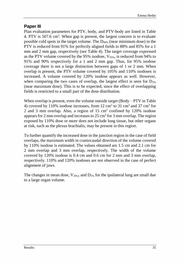
Paper III Plan evaluation parameters for PTV, body, and PTV-body are listed in Table

4. PTV is 507.6 cm3. When gap is present, the largest concern is to evaluate

possible cold spots in the target volume. The D98% (near minimum dose) in the

PTV is reduced from 91% for perfectly aligned fields to 88% and 85% for a 1

mm and 2 mm gap, respectively (see Table 4). The target coverage expressed

as the PTV volume covered by the 95% isodose, V95%, is reduced from 94% to

91% and 90% respectively for a 1 and 2 mm gap. Thus, for 95% isodose

coverage there is not a large distinction between gaps of 1 or 2 mm. When

overlap is present, the PTV volume covered by 105% and 110% isodoses is

increased. A volume covered by 120% isodose appears as well. However,

when comparing the two cases of overlap, the largest effect is seen for D2%

(near maximum dose). This is to be expected, since the effect of overlapping

fields is restricted to a small part of the dose distribution.

When overlap is present, even the volume outside target (Body – PTV in Table

4) covered by 110% isodose increases, from 12 cm3 to 31 cm3 and 37 cm3 for

2 and 3 mm overlap. Also, a region of 15 cm3 confined by 120% isodose

appears for 2 mm overlap and increases to 25 cm3 for 3 mm overlap. The region

exposed by 110% dose or more does not include lung tissue, but other organs

at risk, such as the plexus brachialis, may be present in this region.

To further quantify the increased dose in the junction region in the case of field

overlaps, the maximum width in craniocaudal direction of the volume covered

by 110% isodose is estimated. The values obtained are 1.5 cm and 2.1 cm for

2 mm overlap and 3 mm overlap, respectively. The width of the volume

covered by 120% isodose is 0.4 cm and 0.6 cm for 2 mm and 3 mm overlap,

respectively. 110% and 120% isodoses are not observed in the case of perfect

alignment of jaws.

The changes in mean dose, V20Gy and D2% for the ipsilateral lung are small due

to a large organ volume.


36 Results

Table 4. Plan evaluation measures for PTV, body and body-PTV.

Jaws

2 mm

apart

Jaws

1 mm

apart

Jaws

perfectly

aligned

Fields

overlapping

2 mm

Fields

overlapping

3 mm

PTV V95% (%) 90 91 94 95 95

V105% (%) 16 16 17 22 23

V110% (%) 0.2 0.3 0.4 3.0 4.0

V120% (%) 0.0 0.0 0.0 1.4 2.1

D2% (%) 108 108 109 113 121

D98% (%) 85 88 91 92 92

Dmean (%) 101 101 101 102 103

Body V105% (cm^3) 207 216 224 268 283

V110% (cm^3) 13 13 15 47 59

V120% (cm^3) 0 0 0 15 25

Body-PTV

V95% (cm^3) 503 510 526 547 558

V105% (cm^3) 126 129 133 153 164

V110% (cm^3) 11 11 12 31 37

V120% (cm^3) 0 0 0 5 14

Examples of interpretation: V95% (%) = 90 means that 90% of the organ volume received 95% of the prescribed dose or more. D2% (%) = 108 means that 2% of the organ volume received 108% of prescribed dose or more.

Emma Hedin

Results 37

Paper IV The differences between calculation methods in the values of V5Gy, V10Gy, V20Gy

and V40Gy will be expressed in percentage points. The symbol % is used to

indicate the unit (other common abbreviations are pp or p.p.).

The differences in the ipsilateral lung DVH parameters between AAA and

AXB is illustrated in Figure 12. It is seen that none of the parameters V5Gy,

V10Gy, V20Gy and V40Gy differ more than 3.1%. The smallest differences are seen

for the parameter V20Gy which differ less than 1% for all plans regardless of

FB/DIBH or Tang/LGL. For the tangential treatment plans, decreased lung

density in the DIBH CT-scan synchronize with larger differences between

AAA and AXB for the DVH parameters V10Gy, V20Gy and V40Gy as compared

to the differences between AAA and AXB for the FB CT-scans. For the LGL

plans the same trend is not visible.

The lung densities in the DIBH CT scans for the patient group with both FB

and DIBH CT scans included in this study are distributed between medium to

high density according to the density evaluation of a larger population (157

plans). The comparison of the densities of the larger and smaller group is

shown in Figure 13.

The DVHs for the two low lung-density cases calculated with AAA, AXB and

MC is shown in Figure 14. For those cases the differences in lung DVH

parameters between AAA and AXB is larger than for the group of 14 patients

included in the first part of the study. The largest differences are seen for V10Gy

and V40Gy. For the LGL case AAA calculated 5% higher (lower) value of V10Gy

(V40Gy) compared to AXB. For the tangential case AAA calculated 4% higher

(lower) value of V10Gy (V40Gy) compared to AXB.

In Figure 14 it is seen that AXB comply substantially better with MC than

AAA does. The compliance of the AXB and MC calculations is reassuring.

The two methods both estimate a non-flat DVH and the difference between

AXB and MC is less than 1% for all DVH parameters except V5%.


38 Results

Difference between V5Gy/V10Gy/V20Gy/V40Gy for ipsilateral lung

calculated with AAA and AXB. Left: 5 FB (O) and 5 DIBH (+) loco-regional

treatment plans. Right: 9 FB (O) and 9 DIBH (+) tangential (right) treatment

plans. Each patient has a specific color indicating which O and + that belongs to

that patient (each patient has two CT scans – one FB and one DIBH). Lung

density in isocenter plane on the x-axis.

Emma Hedin

Results 39

Lung density in isocenter plane for patients planned for LGL (left) and

Tang (right) treatments that have treatment plans planned on DIBH CT scans.

The DIBH CT scan lung density for the patients with both FB and DIBH scans are

also shown for comparison. The larger dots (gray) symbolizes the plans chosen

for AAA, AXB and MC comparisons.


40 Results

DVH for ipsilateral lung for a LGL (left) and a Tang (right) breast

cancer treatment plan that were planned on the DIBH CT scan with the lowest

lung densities observed. Dose calculated with AAA, AXB (dose to water),

AXBDtM (dose to medium) and MC.

Emma Hedin

Discussion 41

6 DISCUSSION

Reducing the uncertainties in the estimation of absorbed dose to the patient is

a continuous work. The level of dose accuracy for megavoltage photon beams

in external radiotherapy is discussed in AAPM Report no 85 [35]. The

uncertainty at present (year 2004) is estimated to be 4.3 % (in terms of one

standard deviation) when excluding dose calculation. When 2-3 % uncertainty

in the dose calculation are factored into the total uncertainty the overall

uncertainty is 4.7-5.2 %. A level of 5 % uncertainty is discussed as a desired

and achievable level of accuracy for external radiation therapy [35]. However,

it is recognized in [35] that this level of accuracy in the dose calculation is not

achievable with many existing algorithms. It is for example discussed that

some traditional dose calculation methods produce up to 10 % systematic

errors in the dose in the thorax region when charged particle equilibrium is not

assured. The results in this thesis are in line with this somewhat common

knowledge. The difference between the standard pencil beam algorithms (PB

and PBC) and algorithms that in an approximate way models change in lateral

electron transport (AAA/CC) is illustrated in Paper I. The average decrease in

MLD is up to 5% (10 %) when changing DCA in Eclipse (Oncentra).

LGL breast cancer treatments are considered in three out of four studies (Paper

I, III and IV). This is a treatment with a complex beam geometry, i.e. adjacent

fields. The LGL breast treatment is also giving a considerable lung dose to a

group of patients with long expected survival. The risk for milder grades of

lung tissue complication can be up to 80% as shown in Paper I. Therefore it is

important to work with this type of treatment and continuously decrease the

dose to lung tissue as well as to improve the accuracy of the estimation of risk

for lung tissue complications. The case study on impact of jaw positioning

uncertainty on the dose distribution for a LGL breast treatment (Paper III) was

originally initiated to investigate if there was an effect on lung tissue. In Paper

I it had been found that there was a difference in biological effect between

different DCAs. To be able to conclude on the uncertainties of the estimation

of dose at the planning stage it was desirable to investigate the adjacent fields.

However, the effect on lung dose was small and difficult to assess and the

effects on soft tissue were more apparent.

It is difficult to say how dependent the results of this thesis are on variations in

the exact design of treatments for different treatment centers. It should

especially be noted that the dose distributions of the SBRT lung treatments

studied in this work are calculated on a 3D CT image set. The breathing

motions are taken into account by constructing CTV (the solid tumor and


42 Discussion

diffuse growth at its borders) for each phase of a 4D CT covering the entire

breathing cycle. Then an internal target volume (ITV) is defined that

encompasses all positions of CTV. The PTV is defined as ITV with 5-10 mm

margin. PTV is required to be covered with a certain percentage of the

prescribed dose for the treatment plan to be approved. There are other

techniques for SBRT treatment planning that the results obtained in this work

may not be valid for. For example some hospitals use the mean intensity

projection of all 4D CT phases for dose calculation. Another approach is to use

the mid ventilation scan. The 3D CT used for treatment planning in this work

is a snap-shot of any phase of the breathing cycle.

Comparing clinical DCAs The limitations of clinical DCAs in lung tissue is evaluated for the challenging

clinical situations of small fields (lung SBRT) and low density lung tissue

(LGL delivered with DIBH) in Paper II and IV. For the SBRT Lung treatments

in Paper II AAA calculated an up to 10% higher D98% for PTV compared to

AXB. In Paper IV, for the cases of low lung density, the two investigated

clinical DCAs calculate quite different lung DVHs. AAA underestimates the

DVH for lower doses and overestimates the DVH for higher doses so that V10Gy

(V40Gy) is underestimated (overestimated) by up to 5 percentage points. Since

the value of V10Gy and V40Gy is around 10-20 % for the AAA calculation this

means that the relative effect is large.

The results in Paper I can be used to discuss the differences between DCAs in

terms of biological effect. The study showed that the difference between PB

and CC was for some NTCP model parameters comparable in size to the

uncertainty of the original parameters. The absolute difference in NTCP values

was up to 10 percentage points. The suggested solution to this was to adjust

the NTCP model parameters. NTCP model parameters could be successfully

adjusted to be valid for other algorithms than the reference PB, i.e. the

uncertainty from the mathematical adjustment of the parameters was small

which indicates that the data points in Figure 10 are shifted to a new S-shaped

dose-response curve.

The uncertainty of dose calculation in some clinical situations is much larger

than the desired uncertainty of 2-3%. However, this is sometimes compensated

by the treatment planning criteria. If all plans are calculated erroneously in a

systematic way a treatment planning criterion can still be safe as long as it is

adjusted to the erroneous dose level. This rationale was used for SBRT lung

treatments [36] when both standard pencil beam algorithms (e.g. PB and PBC)

and models that in an approximate way takes changes in lateral electron

transport into account (e.g. CC and AAA) were employed clinically for this

Emma Hedin

Discussion 43

treatment type. In the work cited, recommendation for SBRT lung treatments

are presented. It was concluded that for treatment planning with CC/AAA-type

of algorithms instead of standard pencil beam algorithms the 3x20Gy

fractionation scheme had to be adjusted to 3x18Gy. A similar conclusion was

made in a study comparing PBC and AAA for SBRT lung treatments [37]. This

study resulted in a recommendation of lowering prescribed dose with 10%

when changing DCA from PBC to AAA. In Paper II and IV the transition from

AAA to the principle-based AXB is studied. For this transition, the variation

among patients appears to be larger and without systematics, and the treatment

planning criteria cannot be that easily translated to the new algorithm.

Comparing AXB and MC AXB has been fundamentally investigated in several studies [9, 23, 24, 38-43]

and been found to provide a valid and accurate alternative to Monte Carlo

calculations. In Papers II and IV, the two accurate principle-based dose

calculation methods, AXB and MC, are compared. They are based on the same

measured data but otherwise independent.

The two methods cannot be expected to produce identical results. There are for

example differences in the accelerator head modelling. However, considering

the calculation of dose in the patient geometry, none of those methods is in

principle less accurate than the other. Nevertheless, there are potentially

differences between the methods also in the dose calculation due to

different/inaccurate implementation regarding for example tissue

interpretation or calculation parameters such as resolution of the AXB

calculation and cut-off energy for the explicit tracking of parameters in the MC

calculation.

Compared to AAA, AXB is indeed the clinical DCA presenting the ultimate

compliance with the MC calculations in this work. Still, there are differences

between AXB and MC. AXB calculated for example an up to 6% higher D98%

compared to MC for the SBRT lung treatments in Paper II. The differences

between AXB and MC are also illustrated as a shift in PTV DVHs (Paper II).

In Paper IV the differences between AXB and MC are seen in the high dose

region of the lung DVHs.

One methodological consideration suitable in this context is the choice of

ECUT and the voxel dimensions. According to the recommendations in the

BEAMnrc user’s manual [4] the range of the electrons at ECUT should be less

than 1/3 of the smallest voxel dimension. This means that the lowest density

accurately calculated with the MC method would be 0.0038 g/cm3 for 2 mm

voxels. The lowest densities included in MC calculations are present in the


44 Discussion

DIBH breast treatments in Paper IV (calculated with 2 mm smallest voxel

dimension). In those two cases 8 % (Tang case) and 3 % (LGL case) of the

voxels within the 15 % isodose have density below 0.0038 g/cm3. A less

conservative choice of ECUT was used in for example [44]. The electron range

at ECUT was in that study allowed to be half the smallest voxel dimension or

smaller and the lowest allowed density for 2 mm voxels was therefore 0.0025

g/cm3. The number of voxels with density less than this are 6% (Tang case)

and 2% (LGL case) for the two MC calculated cases of Paper IV. To

investigate the impact of ECUT on the results was beyond the scope of this

study and it is assumed that the choice of ECUT is safe also for the low density

DIBH cases since the number of voxels below the allowed density is relatively

small.

Another methodological issue to discuss when comparing the results of AXB

and MC is the method for tissue segmentation. In the MC calculations sharp

borders are used between tissue types defined by a certain density value. AXB

on the other hand is mixing materials when the density is in an interval between

two tissue types. It would be interesting to do the AXB calculations with the

same tissue density borders as MC to see if the difference in tissue

segmentation methods would affect the dose distributions.

Without further investigations, it is difficult to say which one of the two

methods AXB and MC that is closest to the ‘true’ dose distributions.

Nevertheless, the results from two calculation methods are in this work used

to suggest in which interval the ‘true’ dose is likely to be.

Emma Hedin

Conclusions 45

7 CONCLUSIONS

This work indicates that

- The uncertainties in estimated dose at the treatment planning

stage can be relevant for treatment outcome.

- The uncertainties in estimated dose at the treatment planning

stage is sometimes larger than desired for the clinical

situations investigated.

7.1 Paper-specific conclusions

Paper I The error that can be introduced in NTCP estimates due to differences in dose

calculation algorithms can be of the same magnitude as the confidence

intervals of calculated NTCP values. The use of algorithm-specific NTCP

model parameters can prevent the introduction of this additional uncertainty.

Paper II Two accurate dose calculation methods (AXB and MC) were found to comply

with similarly shaped PTV and GTV DVHs for the challenging situation of

SBRT conventional 3D conformal lung treatment plans. A larger difference

was generally found comparing AAA and AXB. The largest difference

between AAA and AXB was found for the parameter PTV-D98% and was up to

10% (AAA overestimating compared to AXB). The difference in the same

parameter when comparing AXB and MC was found to be up to 6% (AXB

overestimating compared to MC).

A change from AAA to AXB for treatment planning of SBRT lung treatments,

without a change of treatment planning criteria, can increase the dose to the

lung tissue close to the tumor due to an increase of the 100% isodose volume

of up to 20% for some patients.

It was not possible to characterize the treatment plans with larger differences

between AAA and AXB using the patient/plan characteristics studied, i.e. PTV

volume, volume of lung tissue part of PTV, distance from GTV edge to nearest

lung edge, average of lung density in three points two centimeters from PTV,

proportion of PTV edge in lung tissue.


46 Conclusions

Paper III A treatment planning protocol with 1 mm overlap does not considerably

improve the coverage of PTV in the case of erroneous jaw positions causing

gap between fields, but increases the overdosage in PTV and the dose to

healthy tissue, in the case of overlapping fields, for the case investigated.

Therefore, a treatment planning protocol including 1 mm field overlap can be

questioned. Before recommendations are made further investigations are

needed, which should consider, for example, decreased daily setup errors,

hypofractionation, and negative side effects in healthy tissue.

Paper IV For LGL, the difference between AAA and AXB in calculated lung dose was

similar for FB and DIBH, whereas the difference increases with decreased lung

density in DIBH for Tang treatments. For DIBH treatments the underlying CT-

scans for a group of 157 patients show densities in the isocenter plane between

0.08 and 0.3 g/cm3 for LGL and between 0.02 and 0.25 g/cm3 for Tang

treatments. For medium and high lung density, none of the studied lung DVH

parameters differed more than approximately 3%. For the low density cases

the difference can be up to 5%. The least affected lung DVH parameter was

V20Gy which was affected less than 2% for all cases (FB/DIBH, LGL/Tang)

and densities studied.

The AXB and MC predicted similar lung DVHs which is encouraging the use

of AXB. The difference between AXB and MC was less than 1% for all DVH

parameters studied except V5Gy that differed 3%.

To minimize changes in the treatment due to change of algorithm V20Gy is a

suitable parameter for controlling lung dose. V10Gy is a less suitable choice,

since in that case the algorithm change will result in a more conservative

treatment plan regarding lung dose.

Acknowledgement 47

ACKNOWLEDGEMENT

Table 5. List of people that should be acknowledged

ID Thank you…

Anna Bäck and

Roumiana Chakarova

For making this PhD project happen and for all

the time you have invested in me.

Peter Bernhardt For being a helpful co-supervisor

John Swanpalmer For reliable measurements to base the Monte

Carlo model on

Elisabeth Wurzinger For treatment planning

Terapeutisk

Strålningsfysik

For making me feel welcome in the corridor

All fellow PhD students

that I have met

For helpful conversations about life as a PhD

student.

Gunilla For help with administrative matters. And

thank you for always being so kind and

supportive towards all students and PhD

students at Avdelningen för Radiofysik.

Johan Rohlén For the idea of acknowledgement in table

format that I stole from his thesis.

Friends and family For super-important life-supporting

relationships

Hasse For saving me. And buying me vitamin B6.


48 References

REFERENCES

[1] Knöös T, Wieslander E, Cozzi L, et al. Comparison of dose calculation algorithms for treatment planning in external photon beam therapy for clinical situations. Phys Med Biol 2006;51(22):5785-807. [2] Kawrakow I, Mainegra-Hing E, Rogers DWO, Tessier F, Walters BRB. The EGSnrc code system: Monte Carlo Simulation of Electron and Photon Transport. NRC Report PIRS-701. 2016. [3] Berger MJ. Monte Carlo calculation of the penetration and diffusion of fast charged particles. In: Methods in Computational Physics. 1. New York: Academic; 1963. p. 135-215. [4] Rogers DWO, Walters B, Kawrakow I. BEAMnrc Users Manual, NRCC Report PIRS-0509. Ottawa, Canada: National Research Council of Canada, 2009. [5] Verhaegen F, Liu HH. Incorporating dynamic collimator motion in Monte Carlo simulations: an application in modelling a dynamic wedge. Phys Med Biol 2001;46(2):287-96. [6] Storchi PRM, Battum LJv, Woudstra E. Calculation of a pencil beam kernel from measured photon beam data. Physics in Medicine and Biology 1999;44(12):2917. [7] Tillikainen L, Helminen H, Torsti T, et al. A 3D pencil-beam-based superposition algorithm for photon dose calculation in heterogeneous media. Physics in Medicine and Biology 2008;53(14):3821. [8] Ahnesjö A. Collapsed cone convolution of radiant energy for photon dose calculation in heterogeneous media. Medical Physics 1989;16(4):577-92. [9] Vassiliev ON, Wareing TA, McGhee J, Failla G, Salehpour MR, Mourtada F. Validation of a new grid-based Boltzmann equation solver for dose calculation in radiotherapy with photon beams. Phys Med Biol 2010;55(3):581-98. [10] Nilsson E, Berglund M, Palm Å, A method for testing the Linac jaw position of adjacent fields using the EPID. International Conference on Advances in Radiation Oncology (ICARO); 2009; Vienna, Austria: IAEA. [11] Lyman JT. Complication probability as assessed from dose-volume histograms. Radiat Res Suppl 1985;8:S13-9. [12] Kutcher GJ, Burman C. Calculation of complication probability factors for non-uniform normal tissue irradiation: the effective volume method. Int J Radiat Oncol Biol Phys 1989;16(6):1623-30. [13] Niemierko A. A generalized concept of equivalent uniform dose (EUD). Med Phys 1999;26:1100. [14] Källman P, Agren A, Brahme A. Tumour and normal tissue responses to fractionated non-uniform dose delivery. Int J Radiat Biol 1992;62(2):249-62. [15] Rancati T, Fiorino C, Gagliardi G, et al. Fitting late rectal bleeding data using different NTCP models: results from an Italian multi-centric study (AIROPROS0101). Radiother Oncol 2004;73(1):21-32.

References 49

[16] Seppenwoolde Y, Lebesque JV, de Jaeger K, et al. Comparing different NTCP models that predict the incidence of radiation pneumonitis. Normal tissue complication probability. Int J Radiat Oncol Biol Phys 2003;55(3):724-35. [17] Gagliardi G, Bjöhle J, Lax I, et al. Radiation pneumonitis after breast cancer irradiation: analysis of the complication probability using the relative seriality model. Int J Radiat Oncol Biol Phys 2000;46(2):373-81. [18] Rancati T, Wennberg B, Lind P, Svane G, Gagliardi G. Early clinical and radiological pulmonary complications following breast cancer radiation therapy: NTCP fit with four different models. Radiother Oncol 2007;82(3):308-16. [19] De Jaeger K, Hoogeman MS, Engelsman M, et al. Incorporating an improved dose-calculation algorithm in conformal radiotherapy of lung cancer: re-evaluation of dose in normal lung tissue. Radiother Oncol 2003;69(1):1-10. [20] Brink C, Berg M, Nielsen M. Sensitivity of NTCP parameter values against a change of dose calculation algorithm. Med Phys 2007;34(9):3579-86. [21] Chakarova R, Müntzing K, Krantz M, Hedin E, Hertzman S. Monte Carlo optimization of total body irradiation in a phantom and patient geometry. Phys Med Biol 2013;58(8):2461-9. [22] Chakarova R, Krantz M. A Monte Carlo evaluation of beam characteristics for total body irradiation at extended treatment distances. Journal of Applied Clinical Medical Physics; Vol 15, No 3 (2014) 2014. [23] Bush K, Gagne IM, Zavgorodni S, Ansbacher W, Beckham W. Dosimetric validation of Acuros XB with Monte Carlo methods for photon dose calculations. Med Phys 2011;38(4):2208-21. [24] Fogliata A, Nicolini G, Clivio A, Vanetti E, Cozzi L. Dosimetric evaluation of Acuros XB Advanced Dose Calculation algorithm in heterogeneous media. Radiat Oncol 2011;6:82. [25] Ojala JJ, Kapanen MK, Hyodynmaa SJ, Wigren TK, Pitkanen MA. Performance of dose calculation algorithms from three generations in lung SBRT: comparison with full Monte Carlo-based dose distributions. J Appl Clin Med Phys 2014;15(2):4662. [26] Ojala JJ, Kapanen M. Quantification of dose differences between two versions of Acuros XB algorithm compared to Monte Carlo simulations — the effect on clinical patient treatment planning. Journal of Applied Clinical Medical Physics; Vol 16, No 6 (2015) 2015. [27] Schneider W, Bortfeld T, Schlegel W. Correlation between CT numbers and tissue parameters needed for Monte Carlo simulations of clinical dose distributions. Phys Med Biol 2000;45(2):459-78. [28] Ottosson RO, Behrens CF. CTC-ask: a new algorithm for conversion of CT numbers to tissue parameters for Monte Carlo dose calculations applying DICOM RS knowledge. Phys Med Biol 2011;56(22):N263-74.


50 References

[29] Popescu IA, Shaw CP, Zavgorodni SF, Beckham WA. Absolute dose calculations for Monte Carlo simulations of radiotherapy beams. Phys Med Biol 2005;50(14):3375-92. [30] Verhaegen F, Symonds-Tayler R, Liu HH, Nahum AE. Backscatter towards the monitor ion chamber in high-energy photon and electron beams: charge integration versus Monte Carlo simulation. Phys Med Biol 2000;45(11):3159-70. [31] Duzenli C, McClean B, Field C. Backscatter into the beam monitor chamber: implications for dosimetry of asymmetric collimators. Med Phys 1993;20(2 Pt 1):363-7. [32] ICRU. ICRU Report 44: Tissue Substitutes in Radiation Dosimetry and Measurement. Journal of the ICRU: International Commission on Radiaiton Units and Measurements (ICRU), 1988. [33] Locke C, Zavgorodni S. Vega library for processing DICOM data required in Monte Carlo verification of radiotherapy treatment plans. Australas Phys Eng Sci Med 2008;31(4):290-9. [34] DeLuca P, Jones D, Gahbauer R, Whitmore G, Wambersite A. ICRU Report 83: Prescribing, Recording, and Reporting Photon-Beam Intensity-Modulated Radiation Therapy (IMRT). Journal of the ICRU: International Commission on Radiation Units & Measurements (ICRU), 2010. [35] Papanikolaou N, Battista JJ, Boyer AL, et al. Tissue inhomogeneity corrections for megavoltage photon beams. AAPM report no. 85. American Association of Physicists in Medicine (AAPM), 2004. [36] Hurkmans CW, Cuijpers JP, Lagerwaard FJ, et al. Recommendations for implementing stereotactic radiotherapy in peripheral stage IA non-small cell lung cancer: report from the Quality Assurance Working Party of the randomised phase III ROSEL study. Radiation Oncology 2009;4(1):1-14. [37] Herman TDLF, Hibbitts K, Herman T, Ahmad S. Evaluation of pencil beam convolution and anisotropic analytical algorithms in stereotactic lung irradiation. Journal of Medical Physics / Association of Medical Physicists of India 2011;36(4):234-38. [38] Fogliata A, Nicolini G, Clivio A, Vanetti E, Cozzi L. Accuracy of Acuros XB and AAA dose calculation for small fields with reference to RapidArc((R)) stereotactic treatments. Med Phys 2011;38(11):6228-37. [39] Fogliata A, Nicolini G, Clivio A, Vanetti E, Cozzi L. Critical appraisal of Acuros XB and Anisotropic Analytic Algorithm dose calculation in advanced non-small-cell lung cancer treatments. Int J Radiat Oncol Biol Phys 2012;83(5):1587-95. [40] Hoffmann L, Jorgensen MB, Muren LP, Petersen JB. Clinical validation of the Acuros XB photon dose calculation algorithm, a grid-based Boltzmann equation solver. Acta Oncol 2012;51(3):376-85. [41] Misslbeck M, Kneschaurek P. Comparison between Acuros XB and Brainlab Monte Carlo algorithms for photon dose calculation. Strahlenther Onkol 2012;188(7):599-605.

References 51

[42] Rana S, Rogers K. Dosimetric evaluation of Acuros XB dose calculation algorithm with measurements in predicting doses beyond different air gap thickness for smaller and larger field sizes. J Med Phys 2013;38(1):9-14. [43] Rana S, Rogers K, Lee T, Reed D, Biggs C. Dosimetric impact of Acuros XB dose calculation algorithm in prostate cancer treatment using RapidArc. J Cancer Res Ther 2013;9(3):430-5. [44] Aarup LR, Nahum AE, Zacharatou C, et al. The effect of different lung densities on the accuracy of various radiotherapy dose calculation methods: Implications for tumour coverage. Radiotherapy and Oncology 2009;91(3):405-14.


52 References

Appendix 53

APPENDIX

Hedin, E., Bäck, A., Swanpalmer, J. and Chakarova, R. Monte Carlo

simulation of linear accelerator Varian Clinac iX Report MFT-RADFYS

2010:01

MFT – RADFYS 2010:01

Monte Carlo simulation of linear accelerator Varian Clinac iX E. Hedin1, A. Bäck2, J. Swanpalmer2 and R. Chakarova2 (1) Dept. of Radiation Physics, Sahlgrenska Academy, University of Gothenburg, Sweden (2) Dept. of Medical Physics and Biomedical Engineering, Sahlgrenska University Hospital, Gothenburg, Sweden

Copyright

Abstract This report presents methods and results from the development and verification of a Monte Carlo model of a Varian Clinac iX linear accelerator of nominal energy 6 MV. Simulations are made by the BEAMnrc/EGSnrc Monte Carlo code package. Accelerator head components (target, primary collimator, flattening filter, monitor chamber, secondary collimator and jaws) are described in a simplified way according to the technical specifications supplied by Varian Medical Systems. The parameters adjusted in the model are related to the energy and the spatial distribution of the electrons incident on the target. It is assumed that the electrons are monoenergetic, normally incident on the target with Gaussian spatial distribution. The process of parameter tuning and model verification involves two steps. The output from the accelerator head is simulated in one step and the corresponding dose distribution in water is calculated in a subsequent step. Simulated data are compared to measured data visually, quantitatively by directly comparing the data values and by statistical weighting of the differences in a chi2/NDF analysis. The optimum model parameter set is found to be electron energy 5.7 MeV and focal spot width (FSW) 0.1 cm FWHM. The model is verified by depth dose curves and profiles at different depths between 1.5 and 20 cm for field sizes ranging from 2x2 cm2 up to 40x40 cm2. Good agreement within 1% has been achieved between measured and simulated data for nearly all cases. Somewhat larger deviations are detected for profiles at the depth of dose maximum and for the depth dose distribution of 2x2 cm2 field. The accelerator model has been reviewed by international experts and phase space data produced for particular geometries accepted in the IAEA Phase-space database for external beam radiotherapy (http://www-nds.iaea.org/phsp/phsp.htmlx). The model allows simulation of open fields and of wedge fields by applying step-and-shoot method. In a future work, 15 MV nominal energy will be considered and a MLC component will be included to simulate more complex field shapes. Keywords: Monte Carlo methods, simulation, radiation therapy equipment, linear accelerator

Sammanfattning Detta är en internrapport producerad i projektet ”Monte Carlo-baserad NTCP-utvärdering”. Rapporten sammanfattar arbetet med att utveckla en Monte Carlo-modell för en linjäraccelerator (Varian Clinac iX, nominell energi 6 MV) använd för extern strålterapi. På avdelning för strålbehandling används rutinmässigt ett dosberäkningssystem. I dosberäkningssystemet planeras vilka fält och vilken dos som skall ges som behandling. Dosberäkningssystemet levereras med dosberäkningsalgoritmer som med hjälp av approximationer snabbt kan ge ett svar på hur dosfördelningen kommer att se ut. Arbetet med att förfina algoritmerna pågår kontinuerligt. Ett verktyg som kan användas för att bestämma dosens fördelning på ett mer sofistikerat sätt är Monte Carlo-simulering. En väl anpassad Monte Carlo-accelerator modell kan användas vidare för simulering av strålningensväxelverkan i patientensvävnad och utvärdering av precisionen hos dosberäkningsalgoritmen. Speciellt anses Monte Carlo-simuleringar ge mer korrekt dos i komplicerade geometrier. I den aktuella rapporten presenteras metod och resultat vid anpassning av parametrar i en Monte Carlo-model baserad på EGSnrc transport-kod. Processen innefattar två steg, dels att simulera transporten av elektroner och fotoner genom acceleratorhuvudet samt samla in alla partiklar på ett visst avstånd under acceleratorn i en phasespace-fil och dels att simulera vad dosen blir i ett fantom (vattentank) under acceleratorn som träffas av alla partiklar ut phasespace-filen. Vid simulering av transporten av partiklarna genom accelertorn används det för strålterapi avsedda gränssnittet BEAMnrc och vid simulering av dosen i fantom används DOSXYZnrc. Simuleringen av acceleratorhuvudet startar med en stråle elektroner som faller in mot target. De parametrar som anpassas i Monte Carlo-modellen är två egenskaper hos de mot target infallande elektronerna: i) energi (de antas vara monoenergetiska) och ii) vidden på strålen (intensiteten antas vara Gaussiskt fördelad i rummet), som karaktäriseras av FWHM. Olika parameterkombinationer testas och den mest optimala kombinationen väljs ut efter en trial-and-error procedur som slutar när överensstämmelsen mellan uppmätt och simulerad data är god nog. I detta arbete blev de slutgiltiga parametrarna 5.7 MeV i kombination med 0.1cm FWHM. Med dessa parametrar kända är det möjligt att simulera dosen i CT-baserade patientfantom. Nyckelord: Monte Carlo, simulering, strålterapi, linjäraccelerator.

Table of Contents

1 Introduction ..................................................................................... 2

2 Material and methods ..................................................................... 4

2.1 Accelerator head simulation.................................................... 6

2.2 Simulation of in-air profiles ..................................................... 6

2.3 Calculation of dose distributions in water.............................. 8

2.4 Ionisation chamber measurements......................................... 8

2.5 Comparison, measurement-simulation................................... 9

2.6 Finding the optimum parameter combination ...................... 10

2.6.1 In-air simulations................................................................ 10

2.6.2 Dose profiles in water......................................................... 10

2.6.3 Depth dose distributions in water ....................................... 10

2.7 Verifying the optimum parameter combination.................... 11

3 Results........................................................................................... 12

3.1 Finding the optimum parameter combination ...................... 12

3.1.1 In-air simulations................................................................ 12

3.1.2 Dose profiles in water......................................................... 13

3.1.3 Depth dose......................................................................... 13

3.2 Verifying the optimum parameter combination.................... 13

3.2.1 Crossline dose profiles....................................................... 13

3.2.2 Inline dose profiles ............................................................. 27

3.2.3 Depth Dose Curves............................................................ 31

3.2.4 Output Factors ................................................................... 34

3.2.5 Crossline dose Profiles - asymmetric and rectangular fields................................................................................................... 35

4 Remarks and discussion.............................................................. 40

5 References..................................................................................... 41

6 Appendix ....................................................................................... 43


1

List of abbreviations TPS – Treatment Planning System

FWHM- Full Width at Half Maximum (i.e the width of the distribution where the distribution is half of its maximum value)

FSW – Focal Spot Width (in this work characterized by FWHM of Gaussian distribution)

DBS - The variance reduction technique Directional Bremsstrahlung Splitting

SSD - Source Surface Distance

NDF - Number of Degrees of Freedom

OAF - Off Axis Factor

SE - Standard Error (Standard deviation of a stochastic variable propagated through a given formula as an estimate of the error of a calculated value of a given physical quantity)

MLC - Multi Leaf Collimator

IMRT - Intensity Modulated Radiation Therapy


2

1 Introduction

Radiation therapy by photons is one of the most effective techniques for cancer treatment. Ionising radiation is used to destroy tumour cells by damaging their DNA, making it impossible for these cells to continue to grow and divide. The tumour mass may spread and infiltrate healthy tissues. The goal of radiation therapy is to damage as many cancer cells as possible, while limiting harm to nearby healthy tissue. Radiation killing of cells is a stochastic process and has a probabilistic nature. Its evolution is determined by random events of energy deposition in a single interaction. However the effect of the radiation on a large collection of cells is deterministic and related to the amount of the mean energy imparted to the medium, i.e. the absorbed dose. Oncologists prescribe different doses depending on the type and stage of the cancer being treated in order to achieve a certain clinical effect. The accuracy of the dose delivery is of great importance. Larger dose causes significant complications in the normal tissue, whereas reduced dose decreases the probability of tumour control. Therefore the treatment is carefully planned. Tumours are diagnosed and localized with 3D imaging techniques and the irradiation of the patient is simulated by advanced software referred to as a treatment planning system (TPS). The calculation includes (i) configuration of the source of the delivered radiation, i.e. the accelerator output and (ii) simulation of the photon and electron transport through the tissue to obtain dose distribution in the patient. Different simplifications and assumptions are needed in TPS algorithms in order to keep balance between the requirements for fast calculations and for sufficient accuracy of the result. The treatment planning system does not model accelerator components. It rather replaces the machine by a set of virtual sources fitting beam output to certain measured data. Semi-empirical algorithms are implemented to carry out photon and electron transport through the patient. Basic idea is that tissue mainly consists of water and one can therefore calculate the absorbed dose in a water phantom. Libraries of pre-calculated energy deposition kernels in water are produced for different elementary geometries like pencil beam and point kernels. Dose values in tissues with deviating electron densities are derived applying correction factors to dose in water. Validation of the results from treatment planning systems is needed, particularly in situations of complex field shapes, inhomogeneous media and interfaces. The Monte Carlo method is the most accurate method for dose calculations in a wide variety of radiation conditions. Characterisation of the particle beam


3

emitted by an accelerator can be addressed as a separate task preceding the simulation of the interactions in the irradiated tissue for external radiation treatment. Typical accelerator assembly includes electron gun injecting electrons into a waveguide where they are further accelerated and delivered into the treatment head in form of high-energy electron pulses. This primary electron beam hits the target producing bremsstrahlung photons. The bremstrahlung photons penetrate a filtering system, beam monitor detectors and beam defining system and exit the accelerator head as a photon beam with desired characteristics. The Monte Carlo modelling of the accelerator head includes the generation of the bremsstrahlung photons and their further transport through the head components. The model is sensitive to the component descriptions, e.g. target thickness and density, primary collimator specifications, shape and density of the flattening filter, etc [Keall2003, Chetty2007, Sheikh-Bagheri2002]. Therefore the technical data embedded in the model are of importance in spite of the simplifications in the component description by combinatorial geometry. The parameters of the primary electron beam, such as the dimension of the spot, the energy and the spatial distribution, are in general unknown. In the Monte Carlo model, they can be initially set according to the manufacturer recommendations. Their values are then adjusted in a trial and verify process, e.g. simulation of the accelerator output assuming certain parameters, calculation of dose profiles and depth dose distribution, comparisons with measured ones, refining the source parameters until the comparison shows acceptable deviations. Different strategies for tuning the parameters of the primary electron beam are reported in the literature. It is investigated in which radiation geometry the effect of a certain parameter dominates and how to determine its value with higher precision. For example, the derivation of best estimates by [Sheikh-Bagheri2002] is based on comparison of calculated and measured values of in-air off-axis factors for large fields together with calculated and measured central axis relative depth-dose curves. The off-axis factors are found to be sensitive to the mean energy of the electron beam and to FWHM of the radial distribution of the beam assumed to be Gaussian and cylindrically symmetric. The depth-dose curves are shown to be sensitive to the electron beam energy, and to its energy distribution, but not sensitive to the FWHM of the electron beam intensity distribution. [Pena2004] concludes that the accelerator model can be commissioned by large field dose profiles only since these are sensitive both to the energy and width of the electron beam. Depth dose distributions are found to be less sensitive to changes in beam energy. Other authors [Sham2008, Scott2009] recommend implementation of output factors of small fields of order 0.5x0.5 cm or less for adjusting the FSW.


4

Published results from Monte Carlo modelling of 6 MV Varian accelerators show variations in the optimal parameter values found. For example, [Sheikh2002] report primary electron energy of 5.7 MeV with 3% energy spread and a FSW of 0.1 cm FWHM as optimum parameters for a high energy machine, [Keall2003] report electron energy of 6.2 MeV with a 3% energy spread and a FSW of 0.13 cm FWHM for a 2100 EX Varian, [Jutemark2005] presents 6.4 MeV energy of a monoenergetic primary electron beam and a FSW of 0.12 cm FWHM as optimal parameters for a Varian Clinac-23EX accelerator. Variations in the derived optimal parameter values are observed even for one and the same accelerator type (see for example the data for Varian 2100 in table III by [Keall2003]). Since free distribution and information exchange of technical data is not allowed by Varian Medical Systems, detailed comparative studies of Monte Carlo models is not possible. Consequently, optimal parameters reported in the literature can not be automatically adopted since they may not be valid outside the particular model used to derive them. In addition the measured data sets used as a reference in the optimisation procedure may differ even for identical accelerators. Thus developing and optimising a Monte Carlo accelerator model locally for each particular machine becomes a necessary basis for performing radiation treatment simulations. This work presents the Monte Carlo model developed for the Varian Clinac iX accelerator at the radiation treatment department at Sahlgrenska University Hospital (treatment room 8).


The Monte Carlo code package BEAMnrc (Graphical User Interface 2.0) [Walters2009] is used to design a model of linear accelerator Varian Clinac iX. Accelerator components considered in a simplified way are the target, primary collimator, flattening filter, monitor chamber, and upper and lower jaws. The model is based on technical data provided by Varian Medical Systems. It should be noted that several densities are not explicitly specified in the documentation obtained and dimensions presented in different drawings and tables are not always consistent. Densities and dimensions of the accelerator components are fixed during the simulations. Optimisation parameters are the energy and the FSW of the primary electron beam. In-air off-axis factors are used as suggested by [Sheikh-Bagheri2002] and comparison is made between calculated and measured water dose profiles at different depths, depth dose curves and output factors for various field sizes. The calculations are performed partly on a local computer with an Intel Core-2 Duo processor (1066MHz FSB, 4MB L2) using Ubuntu operating system and


5

partly on a Linux cluster at the National Supercomputer Centre (NSC), Linkoping, Sweden (operating system CentOS 5 x86_64 and Intel Xeon E5345 processors). The code is run in a parallel mode on the NSC cluster, using several processors for each job. The optimisation procedure includes two main steps, namely accelerator head simulation with radiation field as result followed by calculation of the dose distribution in irradiated water phantom. The radiation field is stored in an intermediate phase-space file containing information about the particle speed, direction and charge/type. The iterative method of optimising the model is shown schematically in Figure 1. Simulations are made for several combinations of electron energy and FSW. Dose distributions of various field sizes are analysed for each parameter combination. The optimum parameter combination is then verified by simulating the field sizes presented in Table 2 section 2.7.

Figure 1: Sketch describing the iterative method of finding the optimum parameter set describing the radiation field.


6

2.1 Accelerator head simulation

A sketch over the accelerator head and schematic boxes symbolizing phase space and the region with dose distribution of interest are shown in Figure 2. The primary electron beam hitting the target is assumed to be monoenergetic, normally incident with a gaussian radial distribution (BEAMnrc: source number 19). The width of the gaussian radial distribution, the FSW, is characterized by FWHM. The global photon and electron cut-off energy is 0.01 MeV and 0.7 MeV respectively. The variance reduction technique named directional bremsstrahlung splitting (DBS) is used. The splitting number is set to 1000 and the electron splitting is performed in the lower layers of the flattening filter as recommended in the BEAMnrc users manual [Walters2009]. Range rejection is turned on with varying ECUTRR (= the minimum energy a charged particle requires to be able to exit the accelerator still having more than 0.7 MeV ). Range rejection is considered for electrons with energy less than 2 MeV (ESAVE_GLOBAL = 2) except for in the target where range rejection is considered for electrons with energies less than 1 MeV. The same range rejection parameters are used for example by [Hasenbalg2008].

2.2 Simulation of in-air profiles

A first estimate of the energy of the electrons incident on the target is found by using the in-air off axis factors as described by [Sheikh-Bagheri2002]. Water-kerma-profiles (collision) are obtained by processing the phase-space file in a modified version of BEAMDP code. The weight of each photon in the phase space is multiplied by its energy, mass-energy-absorption coefficient [Hubbel1995] and one over the cosine of the angle its direction makes with the z-axis. Only the photons from the phase-space file are taken into account. The contaminating electrons are estimated to influence the results with a magnitude comparable to the uncertainty of the method (for uncertainty reasoning see page 12). Collision kerma profiles are normalised to the value at the central axis to obtain off-axis factors. Collision kerma is assumed to be proportional to the signal from an ionisation chamber with a full build-up cap, an assumption based on the principles of small detector cavities in a region of charge particle equilibrium in which the photons are very unlikely to contribute directly to ionisation but more likely via secondary electrons. The in-air off axis method is fast since the step of calculating dose distribution in the water phantom is avoided. The energy of the electrons incident on the target obtained by this method is regarded to be a first coarse estimate because only one distance from the target is considered, namely the distance at which


7

the phase-space is collected. Changes in FSW may influence the value of optimal electron energy found. However, the FSW sensitivity of the in-air factors is smaller compared to the electron energy sensitivity.

Figure 2: Sketch over the accelerator head, phase space collection and region with dose distribution of interest. x/z-plot at y=0 (central axis). Y direction Jaws not visible in this plane when separated.


8

2.3 Calculation of dose distributions in water

The dose profiles in water phantom are calculated using the Monte Carlo code DOSXYZnrc. The depth dose curves are calculated by the CHAMBER module in BEAMnrc code. No range rejection is used in both cases. The electrons are tracked until their energy falls below 0.512 MeV and the photons are tracked until their energy is below 0.010 MeV. The phantom size is large enough to include the irradiation field with 10 cm lateral margin and 10 cm deeper than the last data point. In DOSXYZnrc the region of interest is divided into voxels with dimensions depending on the resolution needed. When simulating dose profiles for fields larger than 4x4 cm2 the central voxels are 1 cm wide (square top area) and the remaining voxels are 0.3 cm wide. In the cases of 4x4 and 2x2 cm2 fields the central voxels are 0.5 cm wide and the remaining ones are 0.5 cm and 0.2 cm wide, respectively. The voxel width in the case of 4x4 cm2 and 2x2 cm2 field sizes is chosen to correspond to the dimensions of the ionisation chambers to make the simulated penumbral region comparable to the measured (in the cases of 4x4 and 2x2 cm2 field sizes the penumbral region constitutes a large part of the field). Because of the measurement uncertainties associated with the size of the detector and its material the smallest field size considered in this work is 2x2 cm2. When performing simulations for several different parameter combinations (see Section 2.6), dose profiles are extracted at 1.5, 5 and 10 cm depth from 0.5 cm high voxels. When verifying the optimum parameter set, dose profiles are calculated at 1.5, 5, 10 and 20 cm depth using 0.5, 0.5, 0.5 and 1 cm high voxels, respectively. The measured dose profiles for 40x40 cm2 field size are half-profiles. Therefore the simulated profiles are in this case averaged over positive and negative x-axis to obtain better statistics. The depth dose (BEAMnrc) values are determined in 0.2 cm high standing cylinders with a radius of 0.75 cm at the central axis, except for the case of 2x2 cm2 field. In the latter case the cylinders are 0.3 cm high with a radius of 0.15 cm.

2.4 Ionisation chamber measurements

The in-air measurements are performed at a source-detector-distance of 100 cm using a cylindrical ionisation chamber (Exradin T2 Spokas Thimble chamber, 0.53 cm3, 4.6 mm diameter of the collecting volume) with a 3 mm thick brass build-up cap to ensure charged particle equilibrium over the measuring cavity. The chamber signal is assumed to be proportional to dose to water at the centre of the chamber. Air crossline profiles (the x-axis direction


9

defined by the lower jaws) are measured with 1.5 cm steps. The measurement at the central axis position is repeated to achieve better precision. No chamber correction is made for changes in temperature and pressure during the process taking between 30 minutes and one hour. The water measurements are performed using cylindrical ionisation chambers as follows. For field sizes larger than 2x2 cm2 the compact chamber CC13, manufactured by Iba Dosimetry is used (0.13 cm3, inner air cavity diameter 0.6 cm). For the field size 2x2 cm2 the PTW Pin-Point (0.015 cm3, inner cavity diameter 0.2 cm, central electrode of steel) chamber is utilized. Source-surface-distance (SSD) is equal to 100 cm in all water measurements except for the case of the asymmetric 10x10 cm2 field. Dose profile for this asymmetric field is measured using the compact chamber CC04 (0.04 cm3, inner cavity diameter 0.4 cm) at SSD=90 cm. The uncertainties in the above described measurements are estimated to be about 0.5%. Regarding the dose profile measurements the uncertainty, expressed in mm, in the penumbra region for small field sizes is estimated to be less than 1 mm. For the field sizes 10x10 cm and 20x20 cm at a depth of 10 cm this uncertainty is estimated to be around 0.5 mm. The uncertainties concerning the depth dose measurements in the build-up region are more difficult to estimate due to, among other things, the lack of charge particle equilibrium in this region as well as the air cavity size of the cylindrical ionization chamber used for the measurements.

2.5 Comparison, measurement-simulation

The measured and simulated dose profiles and depth dose curves are compared visually and in some cases also by two different methods, namely by chi2/NDF (Number of Degrees of Freedom) cost function and by the number of simulated data points deviating more than a given percentage from the corresponding measured data. The value of chi2/NDF is calculated according to the equation:

χ2 /NDF =(s

i− m

i)2

σ i

2

i=1

N

∑ /(N −1)

where mi and si are measured and simulated normalised dose values,

respectively. σi is the standard error of the i-th simulated value and N is the

number of data points compared. NDF is in this case N-1 since σ is estimated using si (for more details regarding the statistics, see the BEAMnrc users manual [Walters2009] or [Walters2002]). Data beyond dose maximum are included in the chi2/NDF evaluation because of the measurement uncertainties in the build-up region.


10

A comparison between simulations in the build-up region is presented in the appendix along with a discussion regarding differences in simulation methods and versions of BEAMnrc code.

2.6 Finding the optimum parameter combination

2.6.1 In-air simulations The field sizes and parameter combinations used for in-air simulations are presented in Table 1. Table 1: Field sizes and parameter combinations used for in-air simulations. The symbol x indicates that simulation is made.

Energy (MeV)

field size (cm2) FSW (cm) 5.2 5.4 5.5 5.6 5.7 5.8 6.0

40x40 0.05 x

40x40 0.1 x

30x30 0.05 x x x x

20x20 0.05 x x x x x

2.6.2 Dose profiles in water Simulations are initially performed for 10x10 cm2 field with fixed electron energy at 6 MeV and varying the FSW from 1 cm to 0.06 cm. Field size 40x40 cm2 is simulated for the following energy/FSW parameter combinations: 5.8 MeV with 0.05 and 0.1 as well as 5.7 MeV with 0.08, 0.1 and 0.15 cm FSW. Field size 20x20 cm2 is simulated for the same parameter combinations except for the combination 5.7 MeV with 0.08 cm FSW. The start values of the parameter combination are based partly on published results for similar accelerators and partly on the analysis of the in-air simulations and measurements. At the stage of parameter optimisation, only crossline dose profiles (x-direction defined by the lower pair of collimators) are analysed.

2.6.3 Depth dose distributions in water Simulations are made for a 10x10 cm2 field when keeping the FSW at a value of 0.06 cm and varying the energy in steps of 0.2 MeV from 5.2 MeV to 6.4 MeV in order to investigate the response of the depth dose curve to energy changes.


11

2.7 Verifying the optimum parameter combination

The optimum parameter combination is verified by comparing simulated and measured crossline profiles for the fields listed in Table 2. Inline dose profiles (y-direction defined by the upper pair of collimators) for 10x10 and 20x20 cm fields are included in the analysis. Table 2: Simulations in BEAMnrc when verifying the optimum parameter combination. In the second column the associated DBS-radius defined at a distance 100 cm from the top of the target is given. In the last column the calculated dose distributions are given.

Field size (cm2) DBS-radius (cm)

2x2 10 depth distribution, profile





10x10* 20,30 profile

x=4,y=20** profile

*Asymmetric, see the explanation below

**Rectangular field

When verifying the optimum parameter set a 10x10 cm2 asymmetric field is simulated with 5 cm offset in x-direction. Results for -5 cm offset are considered to be a mirrored image of these for 5 cm offset. In general, asymmetric fields are essential for treatment plans containing joint fields. A symmetric (around the central axis) but rectangular field with dimensions x=4 cm and y=20 cm is also simulated to further test the performance of the model. Output factors are calculated for the symmetrical fields in Table 2. The output factors are defined as the ratio between the dose at the central axis at 10 cm depth, for a given field size, and the dose at central axis at 10 cm depth for the 10x10 cm2 square reference field. The dose at 10 cm depth is assessed in two different ways, namely, (i) from a fifth grade polynomial fitted to dose values between depth 5 cm and 20 cm and (ii) from the voxel containing the point of interest.


12

3 Results

The phase-space files obtained typically contain about 3.5E8 particles for 20x20 cm2 field size and between 2E8 and 8E8 particles for 30x30 cm2 field size. The relative uncertainty (1 standard deviation) of the in-air simulated values is 0.1% or smaller. Verification profiles in water are obtained by simulation of more than 1E7 histories per cm2 at SSD=100 cm. Phase space particles are recycled 10 to 15 times. Statistical uncertainties of the simulated dose in water vary. Better statistics is provided when verifying the optimum parameter set compared to that during the optimisation procedure.

3.1 Finding the optimum parameter combination

3.1.1 In-air simulations It is found that changing the value of FSW from 0.1 to 0.05 cm does not significantly influence the in-air profiles. The simulated off-axis factors for different energies, fixing FSW at 0.05 cm, are presented in Fig. 3 together with the measured off-axis factors. The off-axis distance is 12 cm and 7.5 cm for 30x30 and 20x20 cm2 field size, respectively. This off-axis distance is chosen to avoid dose gradients. The optimum energy for 0.05 cm FSW is found to be 5.71 and 5.78 MeV for 20x20 and 30x30 cm2 field size, respectively. The error in the determined energy because of uncertainty in the simulated off-axis factors is difficult to determine from the residuals of the linear fit (the few degrees of freedom yield ±0.5 MeV, 95% confidence interval of the energy from LINEST (Excel 2003) and the t-distribution). In order to take into account the uncertainty of the simulated off-axis factors a linear fit is made for maximum simulated off-axis factors (profile value +95% confidence interval) and for the minimum simulated off-axis factor (profile value -95% confidence interval) respectively. The energy difference is 0.06MeV. An error of measured off-axis factors of ±0.25% leads to uncertainty in the determined energy of ±0.07 MeV. Thus the method gives at least ±(0.07+0.06/2)=±0.1 MeV uncertainty in the energy estimate. The energy intervals should not be considered as statistical confidence intervals but rather as precision limits of the method.


13

3.1.2 Dose profiles in water No change in the lateral profiles is found for 10x10 cm2 field when decreasing FSW below 0.1 cm. Moreover, the profiles obtained for the optimum energy of 5.7 MeV from the in-air simulations in combination with FSW 0.1 cm are found to be in compliance with the measured data, see section 3.2.1.

3.1.3 Depth dose Regarding depth dose curves, energies between 5.6 and 6.2 MeV could be considered equally good when compromising between good fit at dose-max and good fit at deeper depths (assuming that the change in depth dose curve due to FSW is negligible). However as shown in Fig. 4 (125 degrees of freedom, depth 3 to 30 cm), the chi2 analysis is clearly pointing out an optimum energy of 6 MeV when 0.06 cm FSW is used.

3.2 Verifying the optimum parameter combination

The optimum parameter set chosen is 5.7 MeV energy of the electrons incident on the target and FSW 0.1 cm FWHM.

3.2.1 Crossline dose profiles Crossline dose profiles (x-direction) are shown in Figs. 5 to 9. All profiles are at the central axis plane. The dose is normalised to the dose at the central axis for each depth. The simulated and measured profiles for 40x40 cm2 field size for the optimum parameter set [5.7 MeV 0.1 cm] are shown in Fig. 5. None of the simulated data points, between x=0 and x=19.75 cm, in Fig. 5a, 5b, 5c and 5d deviate from the measured data more than 1.5%, 1%, 1% and 1.8% of the central axis dose at the given depth, respectively. The deviation should be considered in conjunction with the relative standard errors of the normalised simulated values which, within the actual interval, are between 0.3% and 0.4%. The simulated and measured profiles for 20x20 cm2 field size for the optimum parameter set [5.7 MeV 0.1cm] are presented in Fig. 6. None of the simulated data points between, x=-8.95 and x=8.95 cm in Figure 6a, 6b, 6c and 6d deviate from measured data more than 1.4%, 1%, 1.3% and 1.2% of the central axis dose at the given depth, respectively. The deviation should be considered together with the relative standard errors of the normalised


14

simulated values which, within the actual interval, are between 0.45% and 0.55%. The chosen parameter set [5.7 MeV 0.1 cm] is further verified for field sizes 10x10, 4x4 and 2x2 cm2. These profiles are shown in Figs. 7 to 9. In the case of 10x10 cm2 field size none of the simulated data points between x=-4.25 and x=4.25 cm in Figs. 7a, 7b, 7c and 7d deviate from measured data more than 1.7%, 1%, 1.5% and 1.2% of the central axis dose at the given depth, respectively. The deviation should be considered in conjunction with the relative standard errors of the normalised simulated values. Within the actual interval these are around 0.4%. The profiles for field sizes 4x4 and 2x2cm2 are analysed visually and the simulated penumbra is seen to agree with measured data to within 1 mm except for at 1.5 cm depth for the 2x2 cm2 field and at 1.5 cm and 5 cm depth for the 4x4 cm2 field, where the difference is between 1 and 1.5 mm. This larger difference is observed only in one of the penumbra regions of the field. It should be noted that non centred measured profiles are used in this case.


15

(a)

(b)

Figure 3: Off-axis factors (OAF) plotted against the energy of electrons incident on the target for the field sizes (a) 20x20 cm2 and (b) 30x30 cm2. The dashed line represents the measured value of off-axis factor at 7.5 cm and 12 cm off-axis distance, respectively. The error bars represent the 95% confidence interval of the simulated data points.


16

Figure 4: chi2/NDF for depth dose curves for 10x10 cm2 field plotted against energy of the electrons incident on the target. Focal spot width fixed at 0.05

cm, energy varied between 5.2 and 6.4 MeV. Error bars ( NDF/2*2 )

represented by the size of the data points. NDF=125, depths between 3 and 30 cm.


17

(a)

(b)


18

(c)

(d)

Figure 5: Dose profiles for 40x40 cm2 field size in water phantom at a) 1.5 cm, b) 5 cm, c) 10 cm, d) 20 cm depth. Solid line measured (CC13) and discrete points simulated. The uncertainties of the simulated values (±1SE) are represented by the size of the data points. Deviation between measured and simulated data is less than a) 1.5%, b) 1%, c) 1%, d) 1.8% of the dose at central axis in the range x=0 to 19.75 cm.


19

(a)

(b)


20

(c)

(d) Figure 6: Dose profile for 20x20 cm2 field size in water phantom at a) 1.5 cm, b) 5 cm, c) 10 cm, d) 20 cm depth. Solid line measured (CC13) and discrete points simulated. The uncertainties of the simulated values (±1SE) are represented by the size of the data points. Deviation between measured and simulated data is less than a) 1.4%, b) 1%, c) 1.3%, d) 1.2% of the dose at central axis in the range x=-8.95 to x=8.95 cm.


21

(a)

(b)


22

(c)

(d)

Figure 7: Dose profile for 10x10 cm2 field size in water phantom at a) 1.5 cm, b) 5 cm, c) 10 cm, d) 20 cm depth. Solid line measured (CC13) and discrete points simulated. The uncertainties of the simulated values (±1SE) are represented by the size of the data points. Deviation between measured and simulated data is less than a) 1.7%, b) 1%, c) 1.5%, d) 1.2% of the dose at central axis in the range x=-4.25 to x=4.25 cm.


23

(a)

(b)


24

(c)

(d)

Figure 8: Dose profile for 4x4 cm2 field size in water phantom at a) 1.5 cm, b) 5 cm, c) 10 cm, d) 20 cm depth. Solid line measured (CC13) and discrete points simulated. The uncertainties of the simulated values (±1SE) are represented by the size of the data points.


25

(a)

(b)


26

(c )

(d)

Figure 9: Dose profiles for 2x2 cm2 field size in water phantom at a) 1.5 cm, b) 5 cm, c) 10 cm,d) 20 cm depth. Solid line measured (pin-point, steel electrode) and discrete points simulated. The uncertainties of the simulated values (±1SE) are represented by the size of the data points.


27

3.2.2 Inline dose profiles Inline dose profiles (y-direction) are analysed visually for a 10x10 cm2 and 20x20 cm2 field. The comparison between measured and simulated data is shown in Figs. 10 and 11. All profiles go through the central axis. The dose is normalized to the dose at the central axis for each depth.

(a)

(b)


28

(c)

(d)

Figure 10: Y-direction dose profiles for 10x10 cm2 field size in water phantom at a) 1.5 cm, b) 5 cm, c) 10 cm, d) 20 cm depth. Solid line measured (CC13) and discrete points simulated. The uncertainties of the simulated values (±1SE) are represented by the size of the data points.


29

(a)

(b)


30

(c)

(d)

Figure 11: Y-direction dose profiles for 20x20 cm2 field size in water phantom at a) 1.5 cm, b) 5 cm, c) 10 cm, d) 20 cm depth. Solid line measured (CC13) and discrete points simulated. The uncertainty of the simulated values (±1SE) is represented by the size of the data points.


31

3.2.3 Depth Dose Curves The depth dose verification curves for the optimum parameter set [5.7 MeV 0.1 cm] are shown in Figs. 12 to 16. The dose is normalised (100%) to dose value at 10 cm depth, taken from a fifth grade polynomial fitted to the simulated data points between the depths 5 and 20 cm. In all cases the simulated data points do not deviate more than 1% (of the maximum dose) from the measured data between the depth of dose max and 25 cm, except for in the case of the 2x2 cm2 field (the extreme regarding small field size), in which the deviation at dose maximum is 2.5% of the dose at dose maximum.

Figure 12: Depth dose curve for 2x2 cm2 field size in water phantom. Solid line - measured data (pin-point ionization chamber, steel electrode) and discrete points - simulated data. The uncertainties of the simulated values (±1SE) are represented by the size of the data points.


32

Figure 13: Depth dose curve for 4x4 cm2 field size in water phantom. Solid line measured (CC13) and discrete points simulated. The uncertainties of the simulated values (±1SE) are represented by the size of the data points.



33




34

3.2.4 Output Factors The output factors obtained are presented in Table 3 and 4. Factors based on dose values taken from polynomial fit of the simulated depth dose curve are presented in Table 3. The factors based on voxel doses are presented in Table 4. The measured output factors are presented as well for comparison. The differences between measured and calculated values normalised to the measured value are shown in column 3. In Table 4 the uncertainty of the normalised difference between measured and simulated output factors is presented. It is seen from Table 3 that the simulated output factors do not deviate more than 2.3% from the measured output factors. For field sizes smaller than 20x20 cm2 the deviation is less than 1.65%. Table 3: Results from output-factor calculations based on doses from polynomial fits of depth dose curves. First column specifies field size ratio (symmetrical fields). Column 1: measured output factors. Column 2: simulated output factors. Column 3: Difference between simulated and measured ratios in percent of the measured ratio.

1 2 3

(cm2/cm2) Meas OF Sim OF [sim-meas]/meas*100

2x2/10x10 0.79 0.80 0.16

4x4/10x10 0.86 0.87 0.93

10x10/10x10 1 1 0

20x20/10x10 1.10 1.08 -1.65

40x40/10x10 1.19 1.16 -2.30

x4y20/10x10 0.94 0.94 -0.02

x20y4/10x10 0.92 0.93 0.59


35

Table 4: Table of results from output-factor calculations based on doses taken from single voxels. First column specifies field size ratio (symmetrical fields). Column 1: measured output factors. Column 2: simulated output factors. Column 3: Difference between simulated and measured ratios in percent of the measured ratio. Column 4: Uncertainty (expressed as the standard error) in the quantity given in column 3.

1 2 3 4

(cm2/cm2) Meas OF Sim OF (voxel)

[sim-meas]/meas*100

SE of column 3

2x2/10x10 0.79 0.79 -0.32 1.42

4x4/10x10 0.86 0.87 1.37 0.59

10x10/10x10 1 1 0 -

20x20/10x10 1.10 1.10 -0.60 0.56

40x40/10x10 1.19 1.16 -2.17 0.54

x4y20/10x10 0.94 0.94 -0.02 0.53

x20y4/10x10 0.92 0.93 0.41 0.54

3.2.5 Crossline dose Profiles - asymmetric and rectangular fields The two special cases of lateral profiles are: one asymmetric 10x10 cm2 field and one rectangular 4x20 cm2 field. The diagrams in which measured and simulated data are compared are shown in Figures 17 and 18. The asymmetric field is analysed at two depths, namely 1.5 cm and 5 cm and the rectangular field at 1.5, 5, 10 and 20 cm depths. Measurements are performed for the different asymmetric fields whereas the symmetry of the Monte Carlo model allows for the simulated data to be mirrored and reused.


36

(a)

(b)


37

(c)

(d)

Figure 17: Dose profiles for 10x10 cm2 asymmetric field in water phantom at a) 1.5 cm, b) 5 cm, c) 1.5 cm, d) 5 cm depth. Dots measured (CC04) and x simulated data. Simulated data from a) and b) mirrored in the dose-axis and used in the comparison in c) and d).


38

(a)

(b)


39

(c)

(d)

Figure 18: Dose profile for symmetric but rectangular field 4 cm in the x-direction (crossline) and 20 cm in the y-direction (inline) in water phantom at a) 1.5 cm, b) 5 cm, c) 10 cm, d) 20 cm depth. Solid line measured and discrete points (x) simulated data.


40

4 Remarks and discussion

The parameter optimisation is made with the future utilisation of the model in mind, in particular, to simulate radiation treatment of breast and lung cancer. The model is fitted to produce accurate dose distributions for various field sizes and depths but not perfectly to reproduce a certain single profile or depth dose distribution. For example, the fit of a depth-dose curve is never perfect but a compromise between dose-maximum at correct depth and good fit deeper along the curve. The accuracy of the model should be additionally tested when applied to other radiation treatment situations, e.g. verification of small field characteristics when simulating IMRT treatments. The parameter set finally chosen for modelling of Varian Clinac iX accelerator (treatment room 8 at the radiation treatment department at Sahlgrenska University Hospital) is found to be 5.7 MeV monoenergetic electrons normally incident on the target with a Gaussian spatial distribution with FWHM 0.1 cm. Those parameter values are within the variations of the results obtained by other authors cited in the Introduction. The off-axis distance in the in-air experiment is chosen with intention to avoid large errors from detector positioning in steep gradient regions. In general, the choice of off-axis distance may affect the resulting optimum energy from the in-air simulations. However, in this study the results from the in-air experiment analysis are regarded only as first approximation and we believe that the choice of the off-axis distance does not influence the final parameter set obtained. All simulated data points in the depth dose curves deviate less than 1% of the dose at dose maximum from the measured data, except for the data points around dose max in a 2x2 cm2 field. A maximum deviation of 1% (of the dose in dose maximum) deviation is further fulfilled in all profiles, except for those at 1.5 cm depth, where the maximum deviation is 1.7%, 1.4% and 1.5% for 10x10, 20x20 and 40x40 cm2 field sizes respectively. The simulated output factors for fields smaller than 20 cm could be assessed to within 1.65% of the measured output factors. The output factors could be more correctly assessed by doing a complete simulation of the monitor chamber in the accelerator head. In this way eventual effects due to backscatter to the monitor chamber from the JAWS could be accounted for. [Ding2003] report such approach for a Varian CL2100EX linear accelerator model. The changes in dose to the monitor chamber per incident electron hitting the target for a 6 MV beam when


41

varying field size are in the order of the deviation between measured and simulated data in this work. Future work includes modelling of 15 MV beams and MLC-component to be able to simulate clinical fields with more complicate shapes. The developed model can also be the base for analytical modelling of the accelerator head which would enable simulation of dynamic wedges and IMRT fields with dynamic delivery.

Acknowledgements This work was supported by Jubileumsklinikens Cancerfond, grants 2008:32, 2009:17 and 2009:45

5 References

Aljarrah K et. al. Determination of the initial beam parameters in Monte Carlo linac simulation. Med. Phys. 2006; 33:850-858 Chetty et. Al. ,Report of the AAPM Task Group No. 105: Issues associated with clinical implementation of Monte Carlo-based photon and electron external beam treatment planning, Med. Phys. 2007; 34 (12): 4819-4853. Ding G X. Using Monte Carlo simulations to commission photon beam output factors- a feasibility study. Phys. Med. Biol. 2003; 48:3865-3874 Hasenbalg F. et. al. Vmc++ versus Beamnrc: A comparison of simulated linear accelerator heads for photon beams. Med. Phys. 2008; 35: 1521-1531 Hubbell J.H. and Seltzer S.M. Tables of x-ray mass attenuation coefficients and mass energy-absorption coefficients 1 keV to 20 MeV for elements Z=1 to 92 and 48 additional substances of dosimetric interest. Technical Report NISTIR 5632, NIST, Gaithersburg, MD, 1995. Jutemark B. Monte Carlo based investigation of the influence of accelerator-head geometry on megavolt photon beam quality in radiotherapy. Masters thesis, 2005 Lund University, LUJI-RADFY-EX-1/2005.


42

Keall PJ et. al. Determining the incident electron fluence for Monte Carlo-based photon treatment planning using a standard measured data set. Med. Phys.2003; 30: 574-582 Pena J et. al. Comissioning of a medical accelerator photon beam Monte Carlo simulation using wide-field profiles. Phys. Med. Biol. 2004; 49:4929-4942 Scott AJ, Nahum AE, Fenwick JD. Monte Carlo modelling of small photon fields: quantifying the impact of focal spot size on source occlusion and output factors, and exploring miniphantom design for small-field measurements. Med Phys. 2009;36(7):3132-3144 Sham E et. al. Influence of focal spot width on characteristics of very small diameter radiosurgical beams. Med. Phys. 2008; 35: 3317-3330 Sheikh-Bagheri Daryoush and Rogers D.W.O. Sensitivity of megavoltage photon beam monte carlo simulations to electron beam and other parameters. Med. Phys. 2002; 29: 379-390 Sheikh-Bagheri Daryoush and Rogers D.W.O. Monte Carlo calculation of nine megavoltage photon beam spectra using BEAM code, Med. Phys. 2002; 29: 391-402 Walters B, Rogers D.W.O. and Kawrakow I. Beamnrc users manual. 2009; NRC Report PIRS-0509(A)rev K. Walters B et. al. History by history statistical estimators in the beam code system. Med. Phys. 2002; 29: 2745-2752


43

6 Appendix

Depth dose simulations - build-up region Depth dose distributions are simulated in two different ways denoted A and B: A) by the module CHAMBER in BEAMnrc using version released 2005 B) by DOSXYZ code using version released 2009 and file format .IAEAphsp Simulations by the CHAMBER module are initially made with poor resolution in the build-up region and then a simulation with 1mm resolution between 0.1 and 2 cm depth is performed. The results from method A and B are compared in Figure 19 and 20. The DOSXYZ-simulations are made in 1 cm2 square pixels and the CHAMBER simulations are made in standing cylinders with 0.75 cm radius and 0.5 cm height.

Figure 19: Simulation by the module CHAMBER with poor resolution in the build-up region compared to simulation made with DOSXYZ (x). Difference is seen at shallow depths. Solid line shows measured depth dose (CC13). Beyond dose maximum the two methods/versions overlap. Additional investigation and a literature study is needed to understand the differences in versions and methods and to understand which one is most correct.


44

Figure 20: Simulation by the CHAMBER module with 1 mm resolution in the region 0.1-2cm depth compared to simulation with DOSXYZ (x – the same curve as in Figure 19).Differences seen at shallow depths.


45

Excerpt of BEAMnrc list file


46

Date post:	14-Feb-2019
Category:	Documents
Upload:	lamthuy
View:	217 times
Download:	0 times

Estimation of clinical dose distributions for breast and ... · Estimation of clinical dose...

Documents