47
Estimation of conditional mean squared error of prediction for claims triangle reserving Mathias Lindholm, Stockholm University London October 10, 2018
Estimation of conditional mean squared error ofprediction for claims triangle reserving
Mathias Lindholm, Stockholm University
London October 10, 2018

The presented material is based on the preprint [6] co-authoredwith
I Filip Lindskog
I Felix Wahl
Aim with the talk:
I Provide a unified approach to conditional MSEP calculations
I Provide a computable “distribution-free” MSEP formulaassuming only knowledge of lower order moments
I Give a number of examples on how to apply the method
Outline of the talk:
I Introduce Mack’s definition of conditional MSEP and thegeneral problem with frequentist “estimation error”
I Introduce a randomisation device for assessing the estimationerror – conditional vs unconditional specification
I Derive a simple (semi-) analytical approximation formula forcalculating conditional MSEP which only relies on lower ordermoments
I Examples: Mack’s C-L, ultimo and CDR(k) calculations, ODPC-L etc.
If time allows:
I Relate different notions of parameter uncertainty – frequentist“estimation error” vs Bayesian “parameter uncertainty”
I Discuss model selection for auto-regressive reserving models –FPE and Mallows’ Cp
Conditional MSEP
I Assume that we have a stochastic process St parametrised interms of a parameter vector θ
I Let F0 = σ{St ; t ≤ 0} denote the σ-algebra containing theinformation known up until today generated by the model St
I Let X denote a random quantity of interest which is afunction of the evolution of St for t > 0
I A natural predictor of X is given by
X := h(θ;F0),
where h(θ;F0) := E[X | F0], and where θ corresponds tosome F0-measurable estimator
I X is often referred to as a “plug-in” estimator of X
I We will refer to the function z 7→ h(z ;F0) as the “basis ofprediction”
Conditional MSEP
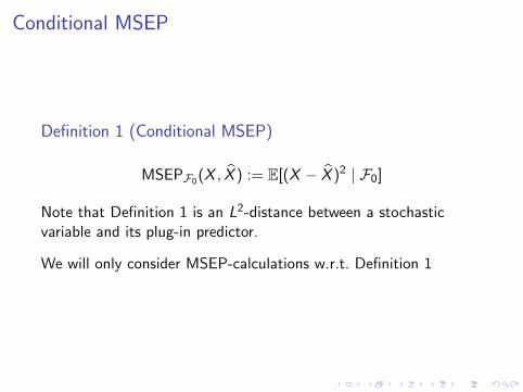
Definition 1 (Conditional MSEP)
MSEPF0(X , X ) := E[(X − X )2 | F0]
Note that Definition 1 is an L2-distance between a stochasticvariable and its plug-in predictor.
We will only consider MSEP-calculations w.r.t. Definition 1
Conditional MSEP
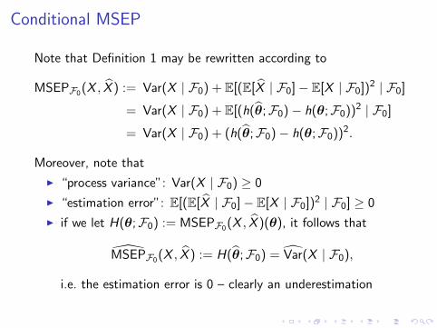
Note that Definition 1 may be rewritten according to
MSEPF0(X , X ) := Var(X | F0) + E[(E[X | F0]− E[X | F0])2 | F0]
= Var(X | F0) + E[(h(θ;F0)− h(θ;F0))2 | F0]
= Var(X | F0) + (h(θ;F0)− h(θ;F0))2.
Moreover, note that
I “process variance”: Var(X | F0) ≥ 0
I “estimation error”: E[(E[X | F0]− E[X | F0])2 | F0] ≥ 0
I if we let H(θ;F0) := MSEPF0(X , X )(θ), it follows that
MSEPF0(X , X ) := H(θ;F0) = Var(X | F0),
i.e. the estimation error is 0 – clearly an underestimation
Conditional MSEP
Although the plug-in process variance may be hard to calculate inpractice, it is usually well defined
We will henceforth focus on the plug-in estimation error
Calculating conditional MSEP
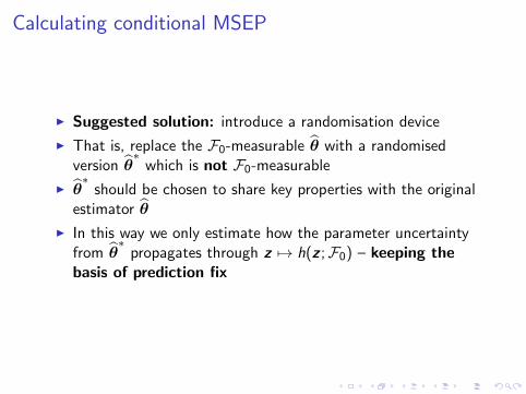
I Suggested solution: introduce a randomisation device
I That is, replace the F0-measurable θ with a randomisedversion θ
∗which is not F0-measurable
I θ∗
should be chosen to share key properties with the originalestimator θ
I In this way we only estimate how the parameter uncertaintyfrom θ
∗propagates through z 7→ h(z ;F0) – keeping the
basis of prediction fix
Calculating conditional MSEP
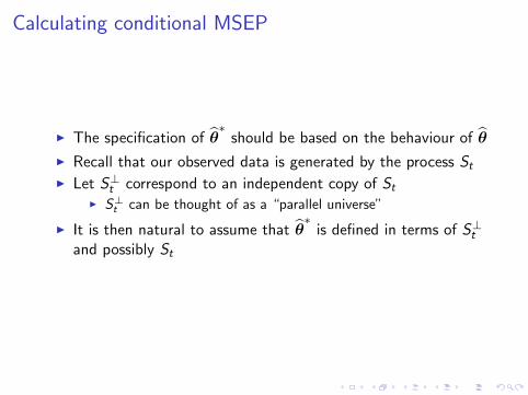
I The specification of θ∗
should be based on the behaviour of θ
I Recall that our observed data is generated by the process StI Let S⊥t correspond to an independent copy of St
I S⊥t can be thought of as a “parallel universe”
I It is then natural to assume that θ∗
is defined in terms of S⊥tand possibly St

Calculating conditional MSEP
Regarding the construction of θ∗
we will make the followingassumption:
Assumption 1
Assume that
X ⊥ θ∗| F0
Definition 2
MSEP∗F0(X , X ) := E[(X − X ∗)2 | F0]
= Var(X | F0) + E[(h(θ∗;F0)− h(θ;F0))2 | F0]
Note that Assumption 1 is fulfilled if we let θ∗
= θ⊥
, i.e. onlyresample based on S⊥t
Calculating conditional MSEP
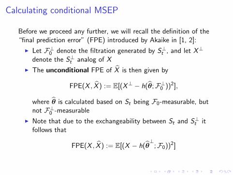
Before we proceed any further, we will recall the definition of the“final prediction error” (FPE) introduced by Akaike in [1, 2]:
I Let F⊥0 denote the filtration generated by S⊥t , and let X⊥
denote the S⊥t analog of X
I The unconditional FPE of X is then given by
FPE(X , X ) := E[(X⊥ − h(θ;F⊥0 ))2],
where θ is calculated based on St being F0-measurable, butnot F⊥0 -measurable
I Note that due to the exchangeability between St and S⊥t itfollows that
FPE(X , X ) := E[(X − h(θ⊥
;F0))2]

Calculating conditional MSEP
I The conditional FPE of X is then given by
FPEF⊥0(X , X ) := E[(X⊥ − h(θ;F⊥0 ))2 | F⊥0 ]
= E[(X − h(θ⊥
;F0))2 | F0]
I That is, given that θ∗
= θ⊥
it holds that
MSEP∗F0(X , X ) = FPEF0(X , X ),
which is a well studied object for model selection forauto-regressive time series models!
Calculating conditional MSEP
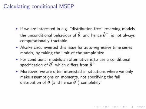
I If we are interested in e.g. “distribution-free” reserving models
the unconditional behaviour of θ, and hence θ⊥
, is not alwayscomputationally tractable
I Akaike circumvented this issue for auto-regressive time seriesmodels, by taking the limit of the sample size
I For conditional models an alternative is to use a conditionalspecification of θ
∗which differs from θ
⊥
I Moreover, we are often interested in situations where we onlymake assumptions on moments, not specifying the fulldistribution of θ (and hence θ
∗) completely

Calculating conditional MSEP
If we make a single first-order Taylor expansion of h(θ;F0) we get
MSEP∗,∇F0(X , X ) := Var(X | F0)
+∇h(θ;F0)′E[(θ∗− θ)2 | F0]∇h(θ;F0)
Note that MSEP∗,∇F0(X , X ) is
I expressed in terms of conditional moments ⇒“distribution-free”
I based on a single first-order Taylor expansion
Calculating conditional MSEP
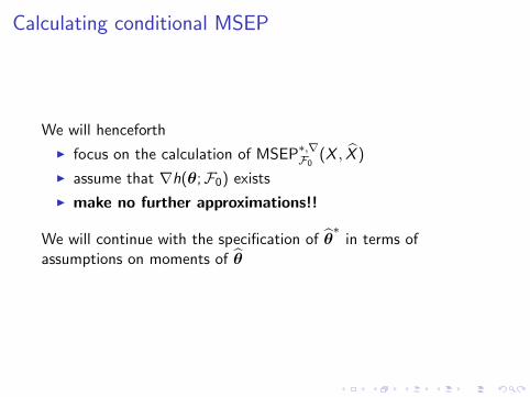
We will henceforth
I focus on the calculation of MSEP∗,∇F0(X , X )
I assume that ∇h(θ;F0) exists
I make no further approximations!!
We will continue with the specification of θ∗
in terms ofassumptions on moments of θ
Specification of θ∗: moment assumptions
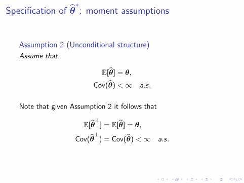
Assumption 2 (Unconditional structure)
Assume that
E[θ] = θ,
Cov(θ) <∞ a.s.
Note that given Assumption 2 it follows that
E[θ⊥
] = E[θ] = θ,
Cov(θ⊥
) = Cov(θ) <∞ a.s.
Specification of θ∗: moment assumptions
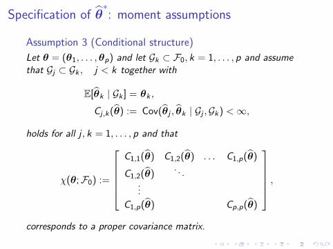
Assumption 3 (Conditional structure)
Let θ = (θ1, . . . ,θp) and let Gk ⊂ F0, k = 1, . . . , p and assumethat Gj ⊂ Gk , j < k together with
E[θk | Gk ] = θk ,
Cj ,k(θ) := Cov(θj , θk | Gj ,Gk) <∞,
holds for all j , k = 1, . . . , p and that
χ(θ;F0) :=
C1,1(θ) C1,2(θ) . . . C1,p(θ)
C1,2(θ). . .
...
C1,p(θ) Cp,p(θ)
,corresponds to a proper covariance matrix.
Specification of θ∗: moment assumptions
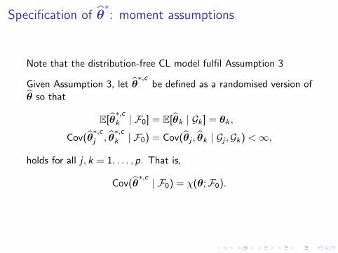
Note that the distribution-free CL model fulfil Assumption 3
Given Assumption 3, let θ∗,c
be defined as a randomised version ofθ so that
E[θ∗,ck | F0] = E[θk | Gk ] = θk ,
Cov(θ∗,cj , θ
∗,ck | F0) = Cov(θj , θk | Gj ,Gk) <∞,
holds for all j , k = 1, . . . , p. That is,
Cov(θ∗,c| F0) = χ(θ;F0).
Specification of θ∗: moment assumptions
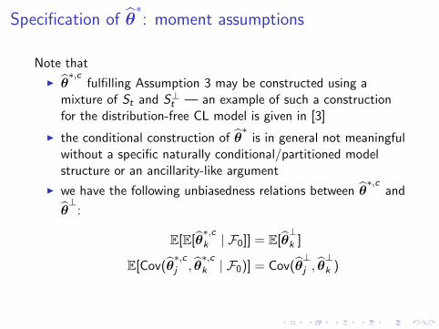
Note that
I θ∗,c
fulfilling Assumption 3 may be constructed using amixture of St and S⊥t — an example of such a constructionfor the distribution-free CL model is given in [3]
I the conditional construction of θ∗
is in general not meaningfulwithout a specific naturally conditional/partitioned modelstructure or an ancillarity-like argument
I we have the following unbiasedness relations between θ∗,c
and
θ⊥
:
E[E[θ∗,ck | F0]] = E[θ
⊥k ]
E[Cov(θ∗,cj , θ
∗,ck | F0)] = Cov(θ
⊥j , θ
⊥k )
Specification of θ∗: moment assumptions
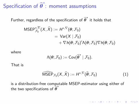
Further, regardless of the specification of θ∗
it holds that
MSEP∗,∇F0(X , X ) := H∗,∇(θ;F0)
= Var(X | F0)
+∇h(θ;F0)′Λ(θ;F0)∇h(θ;F0)
whereΛ(θ;F0) := Cov(θ
∗| F0).
That is
MSEPF0(X , X ) := H∗,∇(θ;F0) (1)
is a distribution-free computable MSEP-estimator using either ofthe two specifications of θ
∗
Specification of θ∗: moment assumptions
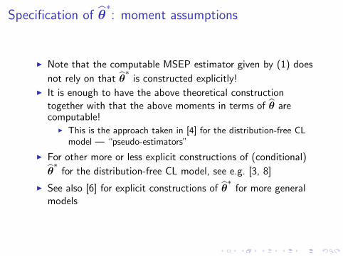
I Note that the computable MSEP estimator given by (1) does
not rely on that θ∗
is constructed explicitly!I It is enough to have the above theoretical construction
together with that the above moments in terms of θ arecomputable!
I This is the approach taken in [4] for the distribution-free CLmodel — “pseudo-estimators”
I For other more or less explicit constructions of (conditional)
θ∗
for the distribution-free CL model, see e.g. [3, 8]
I See also [6] for explicit constructions of θ∗
for more generalmodels

Applications
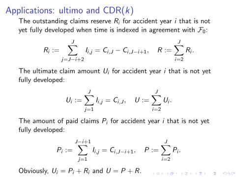
Applications: ultimo and CDR(k)The outstanding claims reserve Ri for accident year i that is notyet fully developed when time is indexed in agreement with F0:
Ri :=J∑
j=J−i+2
Ii ,j = Ci ,J − Ci ,J−i+1, R :=J∑
i=2
Ri .
The ultimate claim amount Ui for accident year i that is not yetfully developed:
Ui :=J∑
j=1
Ii ,j = Ci ,J , U :=J∑
i=2
Ui .
The amount of paid claims Pi for accident year i that is not yetfully developed:
Pi :=J−i+1∑j=1
Ii ,j = Ci ,J−i+1, P :=J∑
i=2
Pi .
Obviously, Ui = Pi + Ri and U = P + R.

Applications: ultimo and CDR(k)
Warm up – still no models:
Ultimo:
I h(θ;F0) := E[U | F0]
I U := h(θ;F0)
I MSEPF0(U, U)(θ) = MSEPF0(R, R)(θ)
I MSEPF0(U, U) = MSEP∗,∇F0
(U, U)(θ)
Applications: ultimo and CDR(k)
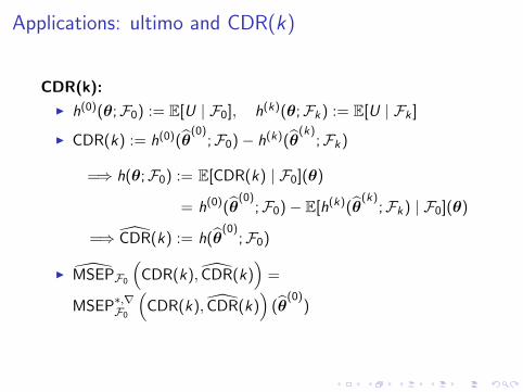
CDR(k):
I h(0)(θ;F0) := E[U | F0], h(k)(θ;Fk) := E[U | Fk ]
I CDR(k) := h(0)(θ(0)
;F0)− h(k)(θ(k)
;Fk)
=⇒ h(θ;F0) := E[CDR(k) | F0](θ)
= h(0)(θ(0)
;F0)− E[h(k)(θ(k)
;Fk) | F0](θ)
=⇒ CDR(k) := h(θ(0)
;F0)
I MSEPF0
(CDR(k), CDR(k)
)=
MSEP∗,∇F0
(CDR(k), CDR(k)
)(θ
(0))
Applications: ultimo and CDR(k)
Note that
I h(0)(θ(0)
;F0) is F0-measurable ⇔ part of the basis ofprediction!!
I MSEP for the ultimo claim amount is consistently definedwith that of CDR(k)
I the definition of MSEP for the CDR(k) differ from those usedin e.g. [3, 4] for the distribution-free CL model — we onlyresample w.r.t. θ in h(θ;F0) := E[CDR(k) | F0](θ)
Applications: the distribution-free CL model
Assume that, for j = 1, . . . , J − 1, there exist constants fj > 0 andconstants σ2j ≥ 0 such that
E[Ci ,j+1 | Ci ,j , . . . ,Ci ,1
]= fjCi ,j ,
Var(Ci ,j+1 | Ci ,j , . . . ,Ci ,1) = σ2j Ci ,j ,
where i = i0, . . . , J, and assume that,
{Ci0,1, . . . ,Ci0,J}, . . . , {CJ,1, . . . ,CJ,J} are independent.
We will focus on MSEP for the ultimo claim amount
Applications: the distribution-free CL model
By using the above defining relations together with the towerproperty of conditional expectations yields
hi (f ;F0) := E[Ui | F0] = Ci ,J−i+1
J−1∏j=J−i+1
fj ,
h(f ;F0) := E[U | F0] =J∑
i=2
hi (f ;F0).
Note that the distribution-free CL model is defined conditionally —
define f∗
conditionally!!
Applications: the distribution-free CL model
That is,
fj =
∑J−ji=i0
Ci ,j+1∑J−ji=i0
Ci ,j
,
and let Bj denote the j first columns of the claims triangle definingF0
Let f∗
be defined so that
E[f ∗j | F0] = E[fj | Bj ] = fj ,
Var(f ∗j | F0) = {Λ(σ;F0)}j ,j = Var(fj | Bj) =σ2j∑J−j
i=i0Ci ,j
,
where {Λ(σ;F0)}i ,j = 0 for all i 6= j .
Applications: the distribution-free CL model
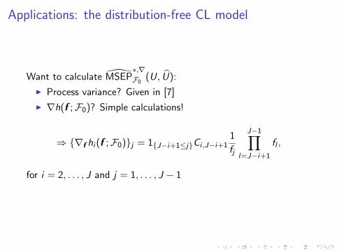
Want to calculate MSEP∗,∇F0
(U, U):
I Process variance? Given in [7]
I ∇h(f ;F0)? Simple calculations!
⇒ {∇f hi (f ;F0)}j = 1{J−i+1≤j}Ci ,J−i+11
fj
J−1∏l=J−i+1
fl ,
for i = 2, . . . , J and j = 1, . . . , J − 1
Applications: the distribution-free CL model
By combining the above and simplifying gives us the following:
Proposition 1
MSEP∗,∇F0
(U, U) from (1) is equal to the MSEP given in [7] for thedistribution-free CL model.
How about if we would use an unconditional specification of f∗?
Unconditional
H − H
Fre
quen
cy
−5 0 5 10 15 200
1000
030
000
Conditional
H − H
Fre
quen
cy
−5 0 5 10 15 20
010
000
3000
0
Unconditional (approx)
H − H
Fre
quen
cy
−5 0 5 10 15 20
010
000
3000
0
Conditional (approx)
H − H
Fre
quen
cy
−5 0 5 10 15 200
1000
030
000
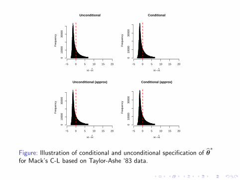
Figure: Illustration of conditional and unconditional specification of θ∗
for Mack’s C-L based on Taylor-Ashe ‘83 data.
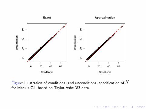
Figure: Illustration of conditional and unconditional specification of θ∗
for Mack’s C-L based on Taylor-Ashe ‘83 data.
Applications: the distribution-free CL model
I It is possible to show that the conditional specification of θ∗
in line with Assumption 3 is an unbiased estimator of theunconditional dito (in fact holds for a wider class of models)
I It is possible to show that both specifications will be closegiven a sufficient amount of data (asym. consistent)
I CDR(k) can be calculated in an analogous manner, but moreinvolved calculations — skip!
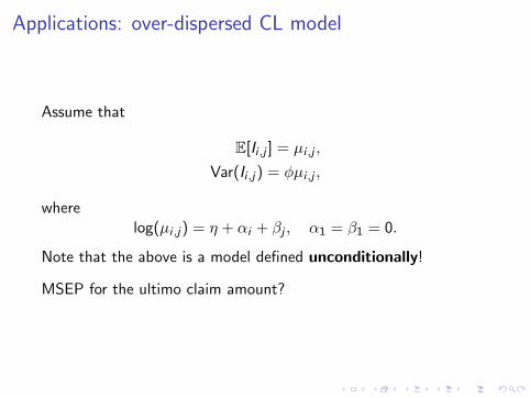
Applications: over-dispersed CL model
Assume that
E[Ii ,j ] = µi ,j ,
Var(Ii ,j) = φµi ,j ,
wherelog(µi ,j) = η + αi + βj , α1 = β1 = 0.
Note that the above is a model defined unconditionally!
MSEP for the ultimo claim amount?

Applications: over-dispersed CL model
hi (θ;F0) = E[Ui | F0] = Ci ,I−i +J∑
j=I−i+1
µi ,j = Ci ,I−i + gi (θ),
where θ = (η, {αi}, {βk}), from which it follows that
∇h(θ;F0) = ∇g(θ)
and similarly it follows that Var(U | F0) = Var(R), where R isindexed in time in agreement with F0
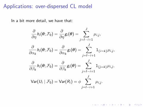
Applications: over-dispersed CL model
In a bit more detail, we have that:
∂
∂ηhi (θ;F0) =
∂
∂ηgi (θ) =
J∑j=I−i+1
µi ,j ,
∂
∂αkhi (θ;F0) =
∂
∂αkgi (θ) =
J∑j=I−i+1
1{i=k}µi ,j ,
∂
∂βkhi (θ;F0) =
∂
∂βkgi (θ) =
J∑j=I−i+1
1{j=k}µi ,j ,
Var(Ui | F0) = Var(Ri ) = φ
J∑j=I−i+1
µi ,j .
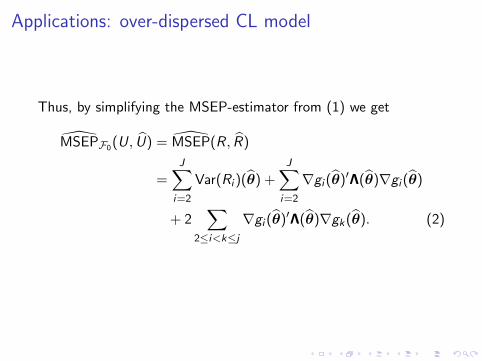
Applications: over-dispersed CL model
Thus, by simplifying the MSEP-estimator from (1) we get
MSEPF0(U, U) = MSEP(R, R)
=J∑
i=2
Var(Ri )(θ) +J∑
i=2
∇gi (θ)′Λ(θ)∇gi (θ)
+ 2∑
2≤i<k≤j∇gi (θ)′Λ(θ)∇gk(θ). (2)

Applications: over-dispersed CL model
Note that
I Λ(θ) is not available analytically, but is approximated whenusing standard GLM-fitting procedures ⇒ (2) issemi-analytical!
I the MSEP-estimator from (2) coincides with that from [5]
I the notion of MSEP reduces to the unconditional FPE — aswanted
Summary
I We have discussed how to calculate the conditional MSEP for(claims triangle based) reserving models
I We introduced a certain randomisation procedure in order toapproach the problems with the estimation error part of thesecalculations
I The introduced randomisation procedure was related toAkaike’s FPE and we showed that FPE = MSEP when usingan unconditional, complete resampling, procedure
I Based on the introduced randomisation procedure we alsosuggested a simple distribution-free formula for calculation ofMSEP based on a single first order Taylor expansion
I The applicability of the approach was illustrated in a numberof examples
References I
Hirotugu Akaike.Fitting autoregressive models for prediction.Ann. Inst. Statist. Math., 21:243–247, 1969.
Hirotugu Akaike.Statistical predictor identification.Ann. Inst. Statist. Math., 22:203–217, 1970.
Markus Buchwalder, Hans Buhlmann, Michael Merz, andMario V Wuthrich.The mean square error of prediction in the chain ladderreserving method (Mack and Murphy revisited).ASTIN Bulletin, 36(2):521–542, 2006.
References II
Dorothea Diers, Marc Linde, and Lukas Hahn.Addendum to the multi-year non-life insurance risk in theadditive reserving model[insurance math. econom. 52(3)(2013) 590–598]: Quantification of multi-year non-lifeinsurance risk in chain ladder reserving models.Insurance: Mathematics and Economics, 67:187–199, 2016.
Renshaw Arthur E.On the second moment properties and the implementation ofcertain glim based stochastic claims reserving models.City University Actuarial Research Paper No. 65, 1994.
Mathias Lindholm, Filip Lindskog, and Felix Wahl.Estimation of conditional mean squared error of prediction forclaims triangle reserving.Preprint, 2018.
References III
Thomas Mack.Distribution-free calculation of the standard error of chainladder reserve estimates.ASTIN Bulletin, 23(2):213–225, 1993.
Ancus Rohr.Chain ladder and error propagation.ASTIN Bulletin, 46(2):293–330, 2016.

Bayesian parameter uncertainty vs frequentist estimationerror
I Let θ∗ denote a random parameter vector and let X bedefined as above
I A Bayesian analog of the conditional MSEP is given by thepredictive posterior variance of X :
Var(X | F0) := E[(X − E[X | F0])2 | F0]
= E [Var (X | θ∗,F0) | F0]
+ E[(h(θ∗;F0)− E[h(θ;F0) | F0])2 | F0
]= Eθ∗|F0
[Var (X | θ∗,F0)]
+ Eθ∗|F0
[(h(θ∗;F0)− E[h(θ;F0) | F0])2
]
Bayesian parameter uncertainty vs frequentist estimationerror
I The estimation/uncertainty part in the two MSEP definitionsare closely related
I Depending on assumptions concerning the a priori distributionof θ∗ you can, depending on model structure, affect the aposteriori distribution providing heuristic guidance on thespecification of θ
∗
I Still, θ∗ is truly random whereas θ∗
is a device to captureuncertainty due to estimation of an unknown parametervector
Distribution-free model selection
I The concept of FPE was originally introduced as a device tobe used for model selection for auto-regressive linear models
I These models are closely related to auto-regressive linearreserving models of the type introduced in e.g. [6]
I The above discussed techniques could hence be used fordistribution-free model selection
I Other approaches to model selection that are closelyconnected to the above notion of MSEP is e.g. Mallows’ Cp,which in our notation, is based on calculating the followingquantity:
Et [(hp(θp;F0)− ht(θt ;F0))2 | F0]
again a situation which can be approached using theintroduced techniques


