ESTIMATION OF DYNAMIC LATENT VARIABLE MODELS USINGSIMULATED NONPARAMETRIC MOMENTS

MICHAEL CREEL

Universitat Autònoma de Barcelona

June 2008

ABSTRACT. Given a model that can be simulated, conditional moments at a trial param-eter value can be calculated with high accuracy by applying kernel smoothing methods toa long simulation. With such conditional moments in hand, standard method of momentstechniques can be used to estimate the parameter. Because conditional moments are cal-culated using kernel smoothing rather than simple averaging, it is not necessary that themodel be simulable subject to the conditioning information that is used to define the mo-ment conditions. For this reason, the proposed estimator is applicable to general dynamiclatent variable models. The estimator is consistent and has the same asymptotic distributionas that of the infeasible GMM estimator based on the same moment conditions. MonteCarlo results show how the estimatod may be applied to a range of dynamic latent variable(DLV) models, and that it performs well in comparison to several other estimators that havebeen proposed for DLV models. An application to weekly spot exchange rate data furtherillustrates use of the estimator.Keywords: dynamic latent variable models; simulation-based estimation; simulated mo-ments; kernel regression; nonparametric estimationJEL codes: C13; C14; C15

Department of Economics and Economic History, Edifici B, Universitat Autònoma deBarcelona, 08193 Bellaterra (Barcelona) Spain. michael.creel@uab.es This research wassupported by grants SEJ 2006-00712/ECON and CONSOLIDER-INGENIO 2010 (CSD2006-00016).

1

2 MICHAEL CREEL

1. INTRODUCTION

Dynamic latent variable (DLV) models are a flexible and often natural way of model-ing complex phenomena. As an example, consider a macroeconomic model. A modelmay specify behavioral rules, learning rules, a social networking structure, and informationtransmission mechanisms for a large group of possibly heterogeneous agents. If the modelis fully specified, it can be used to generate time series data on all of the agents’ actions. Inattempting to use real world data to estimate the parameters of such model, one finds thatreal world data is much more aggregated than the data generated by the model. Typically,individual agents’ actions are not observed - only macroeconomic aggregates are available.From the econometric point of view, many of the variables generated by the model are la-tent. In a dynamic, nonlinear context, this can complicate the econometric estimation of themodel’s parameters.

To fix ideas, consider the general DLV model:

(1) DLV:

yt = rt(yt−1,y∗t ,εt ;θ

)y∗t = r∗t

(yt−1,y∗t−1,εt ;θ

)where t = 1, ...,n. The observable variables are the ky dimensional vector yt , and y∗t is avector of latent variables. Superscript notation is used to indicate the entire history of avector up to the time indicated, so yt−1 ≡

(y′1, ...,y

′t−1)′, and y∗t−1 ≡

(y∗′1 , ...,y∗′t−1

)′. Thereis a vector of independent white noises, εt , with a known distribution. Finally, θ is a vectorof unknown parameters1. This definition closely follows that of Billio and Monfort (2003),with the exception that the same white noise vector enters the equations for both the observ-able and latent variables, to allow for potential correlations in the innovations of the two setsof variables. Calculation of the likelihood function requires finding the density of yn, andas Billio and Monfort make clear, this involves calculating an integral of the same order asn, a problem that is in general untractable. Without the density of the observable variables,analytic moments cannot be computed. Thus, maximum likelihood and moment-based es-timation methods often are not available.

A number of econometric methods have been developed over the last two decades todeal with the complications that may accompany DLV models. These include the simu-lated method of moments (McFadden, 1989; Pakes and Pollard, 1989), indirect inference(Gouriéroux, Monfort and Renault, 1993; Smith, 1993), simulated pseudo-maximum likeli-hood (Laroque and Salanié, 1993), simulated maximum likelihood (Lee, 1995), the efficientmethod of moments (Gallant and Tauchen, 1996), the method of simulated scores (Hajivas-siliou and McFadden, 1998), kernel-based indirect inference (Billio and Monfort, 2003),the simulated EM algorithm (Fiorentini, Sentana and Shephard, 2004), nonparametric sim-ulated maximum likelihood (Fermanian and Salanié, 2004; Kristensen and Shin, 2006) andsimulated nonparametric estimators (Altissimo and Mele, 2007). These methods have been

1The possible presence of observable exogenous variables is suppressed for clarity. The macroeconomic modelof the previous paragraph could be formalized by letting y∗t indicate the vector of all of the agents’ actions, andletting yt be the observed aggregate outcomes.

ESTIMATION OF DYNAMIC LATENT VARIABLE MODELS USING SIMULATED NONPARAMETRIC MOMENTS3

applied to DLV models in a number of contexts. Billio and Monfort (2003) provide numer-ous references for applications.

As noted by Fermanian and Salanié (2004, pg. 702), there often exists a trade-off be-tween the asymptotic efficiency of a method and its applicability to a wide range of models.Simulated maximum likelihood and the method of simulated scores are asymptotically ef-ficient when they can be applied, but this is not the case when the likelihood function orthe score function cannot be expressed as a function of expectations of simulable quanti-ties. Nonparametric simulated maximum likelihood (NPSML) is asymptotically efficientand generally applicable for estimation of static models (Fermanian and Salanié, 2004).Kristensen and Shin (2006) extend the method to some dynamic models. In general, themethod encounters curse-of-dimensionality problems in the case of dynamic models. Pro-posed solutions based upon lower dimensional marginals of the likelihood function lead toa loss of asymptotic efficiency.

The simulated method of moments (SMM) is generally applicable if unconditional mo-ments are used, but foregoing conditioning information may limit the estimator’s ability tocapture the dynamics of the model, and can result in poor efficiency (Andersen, Chung andSorensen, 1999; Michaelides and Ng, 2000; Billio and Monfort, 2003). In the context ofDLV models, the usual implementation of SMM that directly averages a simulator normallycannot be based upon conditional moments, since it is not in general possible to simulatefrom the model subject to the conditioning information. Due to the full specification of themodel, it is easy to simulate a path, yn(θ). However, the elements are drawn from theirmarginal distributions. It is not in general possible to draw from yt |yt−1;θ . To do so, onewould need draws from y∗t |yt−1;θ . If such draws were available, they could be inserted intothe first line of the DLV model given in equation 1, which, combined with a draw from εt ,would give a draw from yt |yt−1;θ . The problem is that the observed value of yt−1 is onlycompatible with certain realizations of the history of the latent variables, y∗t−1, but what isthe set of compatible realizations is not known. For certain types of model it is possible tocircumvent this problem. For example, Fiorentini, Sentana and Shephard (2004) find a wayof casting a factor GARCH model as a first-order Markov process, and are then able to useMarkov chain Monte Carlo (MCMC) methods to simulate from y∗t |yt−1;θ , which is thenfed into a simulated EM algorithm to estimate the parameter. However, for DLV modelsin general, there is no means of simulating from y∗t |yt−1;θ (Billio and Monfort, 2003, pg.298; Carrasco et al., 2007, pg. 544).

Indirect inference is generally applicable, but its efficiency depends crucially upon thechoice of the auxiliary model. The efficient method of moments (EMM, Gallant and Tauchen,1996) is closely related to the indirect inference estimator, and presumes use of an auxiliarymodel that guarantees good asymptotic efficiency, by closely approximating the structuralmodel. This estimator is both generally applicable and is highly efficient if a good auxil-iary model is used, and it is fully asymptotically efficient if the auxiliary model satisfiesa smooth embedding condition (see Gallant and Tauchen, 1996, Definition 1). Satisfyingthis condition is not necessarily an easy thing to achieve. A common practice is to fit a

4 MICHAEL CREEL

semi-nonparametric (SNP) auxiliary model of the sort proposed by Gallant and Nychka(1987), augmented by a leading parametric model that is known to provide a reasonablygood approximation. Andersen, Chung and Sorensen (1999) provide Monte Carlo evidencethat shows the importance of the choice of the auxiliary model. They also note that highlyparameterized auxiliary models often cannot be successfully fit when the sample size is notlarge. It is important to keep in mind that a parsimonious parametric auxiliary model maybe far from satisfying the smooth embedding condition. This can lead to serious ineffi-ciency and to failure to detect serious misspecifications of the structural model (Tauchen,1997; Gallant and Tauchen, 2002). In sum, EMM and indirect inference are clearly attrac-tive methods, given that the sample is large enough to use a rich auxiliary model. Even ifthis is the case, effort and skill are required to successfully use these methods. In the caseof EMM, the documentation of the EMM software package (Gallant and Tauchen, 2004;2007) makes this clear.

The kernel-based indirect inference (KBII) approach suggested by Billio and Monfort(2003) proposes an entirely nonparametric auxiliary model in place of the EMM’s highlyparameterized auxiliary model. The use of kernel regression methods is considerably sim-pler than estimation of models based upon a SNP density with a parametric leading term,since software can be written to use data-dependent rules that tune the fitting process to agiven data set with little user intervention. The consistency of the kernel regression esti-mator ensures a good fit to the data. The main drawback with the KBII estimator is thatthe binding functions are conditional moments of endogenous variables at certain pointsin the support of the conditioning variables. How many such points to use, and exactlywhich points to use require decisions on the part of the econometrician. Billio and Monfortrecognize this problem and propose a scoring method to choose the binding functions.

The simulated nonparametric estimators (SNEs) of Altissimo and Mele (2007) are gen-erally applicable, and are asymptotically efficient when the model is Markovian in the ob-servable variables. This is often an important limitation, since models that are Markovianin all variables are usually not Markovian in a subset of the variables (Florens et al. 1993).When the model is not Markovian in the observable variables, the proposed SNEs are notasymptotically efficient.

This paper offers a new estimator that is applicable to general DLV models. It is a newimplementation of the simulated method of moments (SMM) that allows use of conditionalmoments. Conditional moments are evaluated using nonparametric kernel smoothing ofsimulated data. The estimator is very simple to use since it is just an ordinary GMM esti-mator that uses kernel smoothing to evaluate moment conditions. Because it is a methodof moments estimator, it is not in general asymptotically efficient. However, Monte Carloresults show that moment conditions may be chosen such it performs well in comparisonto other estimators that have been proposed for estimation of general DLV models. Theestimator is referred to as the simulated nonparametric moments (SNM) estimator.

The next section defines the estimator and discusses its properties and usage. The thirdsection presents several examples that compare the SNM estimator to other methods, using

ESTIMATION OF DYNAMIC LATENT VARIABLE MODELS USING SIMULATED NONPARAMETRIC MOMENTS5

Monte Carlo. Section 4 applies the estimator to weekly spot market exchange rate data, andSection 5 concludes.

2. THE SNM ESTIMATOR

2.1. Definition of the estimator. The moment-based estimation framework used in thispaper is standard, and is as follows. The sample is Zn = (yt ,xt)n

t=1, where yt is the re-alization of the ky dimensional vector of endogenous variables Yt , and xt is the realizationof the kx dimensional vector Xt , which is formed of lagged endogenous and exogenousvariables. Define the conditional moments φ(xt ;θ) ≡ E [Yt |Xt = xt ;θ ] (these moments areassumed to exist).

Error functions are of the form

ε(yt ,xt ;θ) = yt −φ(xt ;θ),(2)

An M-estimation approach (Huber, 1964; Gallant, 1987) that down-weights extreme errorswill often be used. In this case, error functions are

(3) ε(yt ,xt ;θ) = tanh(

yt −φ(xt ;θ)2

)Moment conditions are defined by interacting a vector of instrumental variables z(xt) witherror functions:

(4) m(yt ,xt ;θ) = z(xt)⊗ ε(yt ,xt ;θ)

Let the dimension of z(xt) be kz. With kz instruments and kyendogenous variables, thenumber of moment conditions is kykz. Average moment conditions are

(5) mn(Zn;θ) =1n

n

∑t=1

m(yt ,xt ;θ)

To simplify the notation, I will often write mn(θ) in place of mn(Zn;θ). The objectivefunction is

(6) sn(Zn;θ) = m′n(θ)W (τn)mn(θ)

where W (τn) is a weighting matrix that may depend upon prior estimates of nuisance pa-rameters.

Often, φ(xt ;θ) in equations 2 and 3 has a known functional form, in which case esti-mation may proceed using the standard generalized method of moments (GMM). When noclosed-form functional form is available it may be possible to define an unbiased simula-tor φ(xt ,u;θ) such that Eu

[φ(xt ,u;θ)

]= φ(xt ;θ), where the distribution of u conditional

on X = xt is known. If this is so, a simulated error function can be defined by replacingφ(xt ;θ) in equations 2 and 3 with an average of S draws of φ(xt ,us

t ;θ). Doing so, and thenproceeding with normal GMM estimation methods defines the SMM estimator (Gouriérouxand Monfort, 1996, pg. 27). However, in the case of general DLV models, it is often notpossible to simulate subject to the conditioning information Xt = xt , as was discussed above.

6 MICHAEL CREEL

In this case, the SMM estimator cannot be based upon conditional moments as defined inequations 2-5. Estimation by SMM using unconditional moments is still feasible, but theMonte Carlo evidence cited above has shown that this approach often has poor efficiency,due to the fact that unconditional moments provide little information on the dynamics of aDLV model.

The fundamental idea of the simulated nonparametric moments (SNM) estimator pro-posed here is to replace the expectations φ(xt ;θ) that are used to define error functionsin equations 2 and 3 with kernel regression fits based on a very long simulation from themodel. Kernel regression (also known as kernel smoothing) is a well-known nonparametrictechnique for estimating regression functions of unknown form (Robinson, 1983; Bierens,1987; Härdle, 1991; Li and Racine, 2007). Its application here is entirely standard, exceptfor the use of simulated data.

In the following, tildes will be used to indicate simulated data or elements that dependupon simulated data. Let ZS(θ) = (ys(θ), xs(θ))S

s=1 be a simulated sample of size S fromthe model, at the parameter value θ . Kernel regression may be used to fit φ(xt ;θ), usingthis simulated data

(7) φ(xt ; ZS(θ)) =S

∑s=1

wsys(θ)

where the weight ws is

(8) ws =K(h−1

S [xt − xs(θ)])

∑Ss=1 K

(h−1

S [xt − xs(θ)])

To avoid notational clutter, I will often write φ(xt ;θ) in place of φ(xt ; ZS(θ)) in the follow-ing. Note that the same weight ws applies to each element of ys (which is a kY -vector). Tospeed up computations, one should not separately fit each of the kY endogenous variables,but rather employ a specialized kernel fitting algorithm that saves the weights across vari-ables. Since xt is of dimension kx, which is in usually greater than one, the kernel functionK(·) is in general multivariate. The bandwidth (or window width) parameter is hS. Note thatthe kernel regression fit can be evaluated at xt without requiring that the simulated sequencecontain any realizations such that xs = xt . What is required for a good fit at xt is that therethere be a large number of realizations that are "close enough" to xt .

The SNM estimator follows the standard moment-based estimation framework, exceptthat the kernel fit φ(xt ;θ) is used in place of the expectation of unknown form, φ(xt ;θ). Tobe explicit, the SNM estimator is based on error functions of the form

ε(yt ,xt ; ZS(θ)) = yt − φ(xt ;θ),(9)

or

(10) ε(yt ,xt ; ZS(θ)) = tanh

(yt − φ(xt ;θ)

2

)

ESTIMATION OF DYNAMIC LATENT VARIABLE MODELS USING SIMULATED NONPARAMETRIC MOMENTS7

The moment function contribution of an observation is

(11) m(yt ,xt ; ZS(θ)) = z(xt)⊗ ε(yt ,xt ; ZS(θ))

Average moment conditions are

(12) mn(Zn; ZS(θ)) =1n

n

∑t=1

m(yt ,xt ; ZS(θ))

To clarify the notation, I will often write mn(θ) in place of mn(Zn; ZS(θ)). The objectivefunction that defines the SNM estimator is

(13) sn(Zn; ZS(θ)) = m′n(θ)W (τn)mn(θ)

where W (τn) is a weighting matrix that may depend upon prior estimates of nuisance pa-rameters. The SNM estimator is the minimizer of this function:

(14) θn = argmin sn(Zn; ZS(θ)).

To simplify the notation, the objective functions that define the GMM and SNM estimatorswill often be written as sn(θ) and sn(θ), respectively.

2.2. Properties of the SNM estimator. This section deals with the consistency and as-ymptotic normality of the SNM estimator. The proof offered here is high level, in the senseAssumptions 2 and 3 below are made without detailing assumptions on the DLV model ofequations 1 that would cause them to hold. Given a more concrete formulation of the DLVmodel, one could provide more low level assumptions that would imply Assumptions 2 and3. This is not done here since the intention is not to focus on any particular model.

The first assumption defines the true parameter value:

Assumption 1. The sample Zn = (yt ,xt)nt=1 is generated by the DLV model of equations

1, at the true parameter value θ0.

Next, assume that the chosen endogenous variables, conditioning variables, and instru-ments define a GMM estimator that is consistent and distributed asymptotically normally.Of course, this estimator normally is not feasible if the SNM estimator is under considera-tion, but abstractly, it is assumed to have the usual desirable properties:

Assumption 2. Let θn = argminsn(Zn;θ) where sn(Zn;θ) is defined in equation 6. This(infeasible) GMM estimator is consistent: θn

a.s.→ θ0 and asymptotically normally distributed:√

n(

θn−θ0

)d→ N (0,V∞) where V∞ is a finite positive definite matrix.

Next, assume that the kernel regression estimator used to define the SNM error functionsin equations 9 and 10 is strongly consistent, uniformly over the conditioning variables, asthe length of the simulation, S, tends to infinite:

Assumption 3. φS(xt ;θ) a.s.→ φ(xt ;θ), for almost all xt , as S→ ∞.

A number of results can justify this assumption, depending on the nature of the model.For example, supposing that the data Zn generated by the DLV model constitutes a strictlystationary α-mixing sequence, Lu and Cheng (1997) show that Assumption 3 holds.

Assumption 4. The parameter space Θ over which minimization is done is compact.

With a compact parameter space, the convergence of Assumption 3 holds uniformly overΘ.

Assumption 5. The simulation length, S, is greater than the sample size, n.

This will allow us to focus on asymptotics as n tends to infinity, without separately deal-ing with S.

Assumption 6. The instruments are bounded in probability: z j(xt) = Op(1), j = 1,2, ...,kz.

Proposition 1. This is being worked on

Proof of Proposition 1: See the Appendix.By making S suitably large, it is possible to make φS(xt ;θ) as close as is desired to the

true moment φ(xt ;θ). In principle, S could be chosen large enough so that the differencesbetween the error functions in equations 2 and 9 (or the M-estimation analogues in equations3 and 10) are smaller than the machine precision of a digital computer. If this is the case,the SNM estimator essentially is the infeasible GMM estimator.

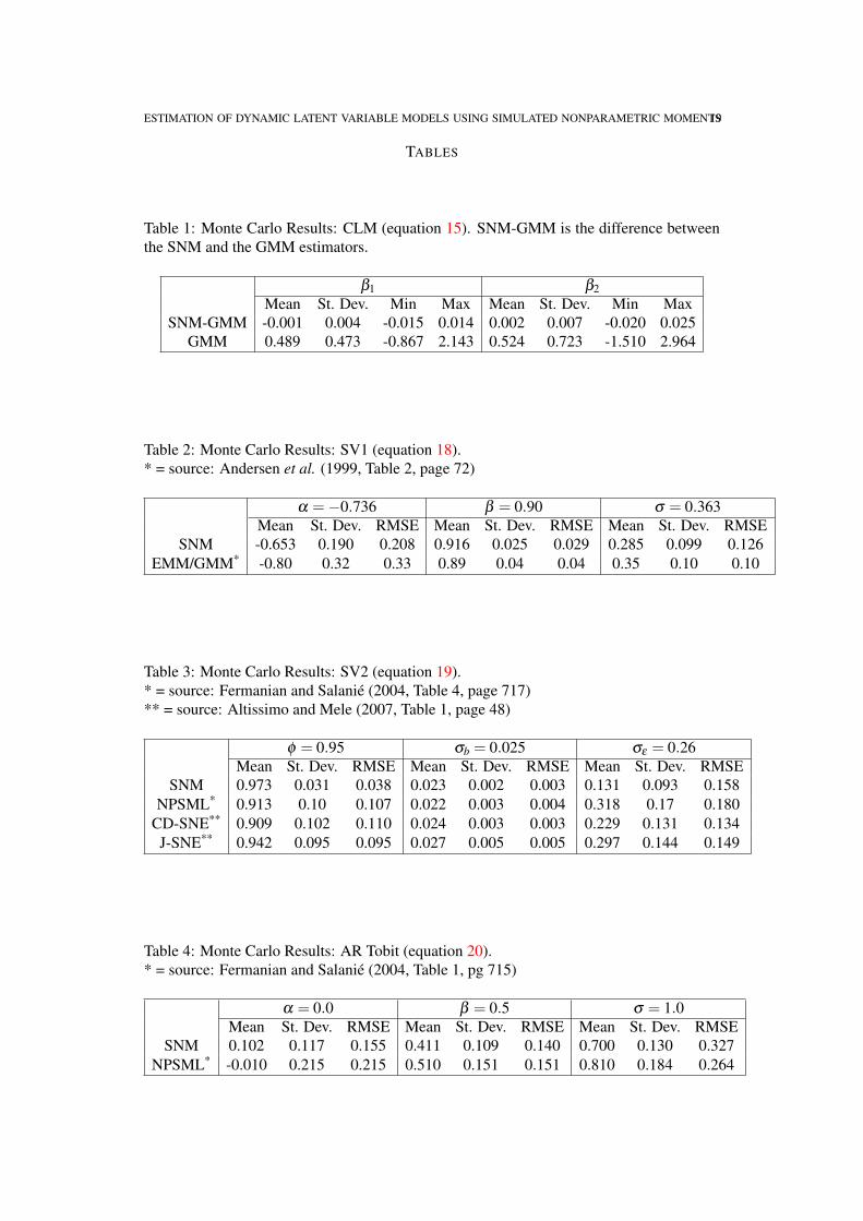
A simple Monte Carlo exercise illustrates this point. Samples of size n = 30 were gener-ated using the classical linear model (CLM)

(15) CLM:

y = β1 +β2x+ ε

x ∼U(0,1)

ε ∼ N(0,1)

The parameters β1 and β2 were randomly drawn (separately) from U(0,1) distributions ateach of 1000 Monte Carlo replications. The maximum likelihood (ML) estimator is theordinary least squares (OLS) estimator obtained by regressing y on a constant and x. TheML estimator may be thought of as a GMM estimator that uses the single (ky = 1) errorfunction εt = yt −β1−β2xt and the instruments (1,xt). The SNM estimator was applied,using the endogenous variable yt , the conditioning variable xt and instruments (1,xt). Thesimulation length was S = 500000, and the hS = S−1/(4+kx) is chosen using a simple rule-of-thumb procedure 2. A standard Gaussian kernel was used.

Table 1 gives results that compare the distribution of the difference between the SNMand GMM estimators to the distribution of the GMM estimator, over the 1000 Monte Carloreplications. We can see that the difference between the two estimators is distributed tightlyaround zero, and that the dispersion of the difference is much less than that of the GMMestimator. If the value of the SNM estimator is regressed on a constant, the value of the

2See Li and Racine, 2007, pg. 66. Recall that kx is the number of conditioning variables (kx = 1 in the presentcase).

GMM estimator, and the value of the true parameter, the results are (estimated standarderrors in parentheses), for the constant, β1:

β1(SNM) =−0.00106912(0.00023012)

+ 1.00292(0.00030566)

β1(GMM)−0.00267236(0.00050332)

β1

For the slope, β2, we obtain

β2(SNM) = 2.50475e-5(0.00038392)

+ 1.00389(0.00029626)

β2(GMM)−0.000178451(0.00073023)

β2

In both cases, R2 is higher than 0.999. We see that the SNM and GMM estimators areessentially identical, independent of the true parameter value.

Recall that the GMM estimator is fully asymptotically efficient for this model. Compar-ing root mean squared error (RMSE) over the 1000 Monte Carlo replications, the RMSEof the SNM estimator relative to RMSE of the fully efficient GMM estimator is 1.003 inthe case of β1, and 1.004 in the case of β2. Since the estimators are essentially the same,so are their efficiencies. The SNM estimator can be very efficient if moment conditions arewell-chosen.

These results illustrate the fact that when a long enough simulation is used the SNMestimator essentially is the GMM estimator that uses the same endogenous variables andthe same conditioning variables. The GMM estimator adds information about the functionalform of the moment condition, while the SNM estimator fits it nonparametrically. WhenS is large enough, the nonparametric fit is so good that the SNM estimator is practicallyidentical to the GMM estimator. Of course, one would only use the SNM estimator whenthe functional form of φ(xt ;θ) is unknown, so that the GMM estimator is infeasible.

2.2.1. Inference and estimation of the optimal weight matrix. Given that the SNM estimatorhas the same asymptotic distribution as the infeasible GMM estimator, one can use standardmethods and asymptotic results for GMM estimators to make statistical inferences with theSNM estimator. For example, an overidentified model’s specification may be tested usingthe familiar χ2 test based upon n sn(θn), (assuming that an optimal weight matrix is used).

The asymptotic covariance matrix of the moment conditions is

(16) Ω = limn→∞

E[nmn(θ 0)mn(θ 0)′

]where mn(θ 0) is defined in equation 12. A consistent estimator of this matrix is neededif one wishes to use an efficient weight matrix, and in any event it is also needed for hy-pothesis testing. In the ordinary GMM setting without a fully simulable model, this covari-ance matrix must be estimated using only the sample data, which requires use of one ofthe kernel-based heteroscedasticity and autocorrelation-consistent covariance matrix esti-mators (for example, that of Newey and West, 1987). It is well-known that inferences basedupon such covariance estimators can be quite unreliable (Hansen, Heaton and Yaron, 1996;Windmeijer, 2005).

10 MICHAEL CREEL

In the context of the SNM estimator, or any other moment-based estimator that relieson a fully simulable model, is is possible to estimate Ω though Monte Carlo. The momentconditions of equation 12 may be simulated many (say, R) times, given an initial consis-tent estimate of the model’s parameter. Following notation previously used, a simulation oflength equal to the real sample size (n), at the initial consistent estimate θ may be repre-sented by Zn(θ) =

(yt(θ), xt(θ)

)n

t=1. We may generate R such samples of size n, and

for each of them calculate simulated moment conditions as in equation 12. The rth suchreplication (r = 1,2, ...,R) is(˜mn

)r= mn(

(Zn(θ)

)r;(

ZS(θ))

r)

where(

Zn(θ))

rand

(ZS(θ)

)r

are independent simulations of lengths n and S, respectively.

Let m be the average of the R draws of(˜mn

)r, and define vr =

(˜mn

)r−m. Then Ω of

equation 16 may be estimated using

(17) Ω =nR

R

∑r=1

vrv′r

This procedure requires R evaluations of the moment conditions, where R is a reasonablylarge number. This is not unduly burdensome computationally, since a large number ofevaluations of the moment conditions is done during the course of iterative minimization ofthe objective function sn(θ) of equation 13. If it is computationally feasible to minimizesn(θ), then it is also computationally feasible to estimate Ω using the above procedure. Thismethod has the advantage that it obviates the need for decisions regarding lag lengths, pre-whitening and so forth that attend the use of kernel-based covariance matrix estimators thatuse only the sample data.

To provide some rudimentary evidence of this covariance estimator’s performance, aMonte Carlo study of 1000 replications was done. Data was generated using the classicallinear model of equations 15. The SNM estimator was applied using a sample size n = 30,

a simulated sample size S = 10000, and R = 1000 draws were used to estimate Ω for eachof the 1000 Monte Carlo replications. The true value of Ω for this model is Ω11 = 1,Ω12 = 1/2, Ω22 = 1/3. Over the 1000 Monte Carlo replications, the mean and standarderrors (in parentheses) of the replications of Ω are Ω11 : 1.036 (0.048), Ω12 : 0.517 (0.025),Ω22 : 0.343 (0.015). For this simple model, the covariance of the moment conditions isestimated quite well using the proposed simulation method. The small upward bias is likelydue to the shortness of the simulation length, S. More careful investigation of the empiricalperformance of this covariance matrix estimator is left for future work.

Once the covariance of the moments is estimated, hypothesis testing may then be doneusing standard results for GMM estimators with an inefficient weight matrix, or a secondround of estimation may be done using the inverse of Ω to estimate the efficient weightmatrix.

ESTIMATION OF DYNAMIC LATENT VARIABLE MODELS USING SIMULATED NONPARAMETRIC MOMENTS11

2.2.2. Choice of the kernel and the bandwidth. To implement the SNM estimator, the ker-nel function K(·) in equation 8 must be chosen, as must the bandwidth, hS. Regarding thekernel, in this paper attention is restricted to local constant kernel regression estimators (Liand Racine, 2007). In this context, much theoretical and empirical evidence shows that thechoice of the particular kernel function has relatively little effect on the results, as long asthe bandwidth parameter is chosen appropriately, given the kernel (Li and Racine, 2007).For this reason, this paper uses Gaussian product kernels exclusively, accompanied by priorrotation of the data to approximate independence of the conditioning variables. Gaussianproduct kernels lead to error functions that are continuous and relatively smooth in the pa-rameters, which facilitates iterative minimization. Kernels such as the radial symmetricEpanechnikov are relatively inexpensive to compute, but can lead to error functions that arediscontinuous in the parameters, which complicates minimization of the objective functionthat defines the SNM estimator. This paper leaves the possibility of SNM estimation basedon local linear or local polynomial kernel methods for future work.

Given the kernel function, the bandwidth must be chosen. The bandwidth does have animportant effect upon the quality of the kernel regression fit. Too large a bandwidth over-smooths the data, and induces a fit with low variance but high bias. Too small a bandwidthhas the opposite effect. The bandwidth may be chosen using data-driven methods such asleave-one-out cross validation, or by using rule-of-thumb methods that are known to workwell in certain circumstances but may perhaps perform poorly in others. In this paper, asimple rule-of-thumb method is used throughout, since investigation of data-driven methodswould add substantially to the computational burden of the Monte Carlo work presentedbelow. It is expected that use of a data-driven method would improve the performance ofthe SNM estimator. Future work will address this issue more carefully.

2.2.3. Computational issues. Estimation of a complicated model using long simulationmay become computationally burdensome, since kernel smoothing is a computationallyintensive procedure. In common with normal GMM estimators (Chernozhukov and Hong,2003, especially pp. 296-298), the SNM objective function is not globally convex, so oneneeds to take care to find the global minimum by using estimation methods such as simu-lated annealing (Goffe et al., 1994). One may seek to use data-based methods to choose thebandwidth, as well. These factors imply that use of the SNM estimator is computationallyintensive. However, kernel regression fitting, which is at the heart of the SNM estimator,is easily parallelized (Racine, 2002; Creel, 2005), as is Monte Carlo work (Creel, 2007).The widespread availability of multicore processors is an invitation to take advantage ofparallelization opportunities in econometric work. All of the results reported in this paperwere obtained on a computational cluster that provided a total of 16 CPU cores, runningthe PelicanHPC distribution of GNU/Linux3. To give an idea of the computational demands

3PelicanHPC is described at http://pareto.uab.es/mcreel/PelicanHPC. It is the evolution of theParallelKnoppix distribution of GNU/Linux, which was described in Creel (2007).

12 MICHAEL CREEL

associated with the SNM estimator, the results reported in this paper required roughly 10days of computational time on this cluster.

3. MONTE CARLO RESULTS

This section presents Monte Carlo results that compare the SNM estimator to other esti-mators that have been proposed for estimation of DLV models. The intention is to show thatthe SNM estimator can be used to successfully estimate a variety of DLV models, that theSNM estimator performs well in comparison to alternative estimators, and to give examplesof how the moment conditions that define the SNM estimator may be chosen.

All of the simulations shared the following features. The SNM estimator was imple-mented using a Gaussian product kernel. Both the simulated and real conditioning variableswere transformed in two ways before applying the Gaussian kernel. First, they were individ-ually shifted and scaled so that their minima and maxima were -4 and 4, respectively. This”compactification” ensures that trial parameter values cannot generate extreme outliers thathave no neighbors close enough to generate a positive weight when evaluating the kernel.This transformation is done to provide numeric stability, which is needed when many MonteCarlo replications of a nonlinear minimization are to be done. The second transformation isto multiply by the inverse of the Choleski decomposition of the sample covariance matrix ofthe real conditioning variables (after the first transformation), before applying the Gaussiankernel. The transformed variables are thus more nearly independent, which makes use of aproduct kernel more reasonable. In all cases the rule of thumb bandwidth h = S−1/(4+kx) wasused, where kx is the number of conditioning variables. Likewise, the M-estimation errorfunctions of equation 3 were always used, since they were found to provide good numericalstability during the course of many nonlinear minimizations. Future work could explore ef-ficiency issues with regard to the choice of error functions. In all cases a simulation lengthof S = 10000 was used, to limit the computational burden. For the same reason, only firstround estimates using an identity weight matrix were calculated. For each problem, 500Monte Carlo replications were calculated. Because the SNM objective function is not nec-essarily globally convex, care is needed to ensure that the global minimum of the objectivefunction is found. For each Monte Carlo replication, minimization was done using an initialcourse of simulated annealing that involved at least 300 trial values for the parameter vector,followed by use of a quasi-Newton method iterated to convergence.

3.1. Stochastic volatility. Andersen, Chung and Sorensen (1999) provide Monte Carloresults comparing EMM with GMM in the context of a simple stochastic volatility model.Adapting the notation to conform with the general DLV model of equation 1, the model is

(18) SV1:

yt = exp(y∗t /2)ε1t

y∗t = α +βy∗t−1 +σε2t

where the white noise εt = (ε1t ,ε2t)′ is distributed i.i.d. N(0, I2). The stochastic volatility

model of equation 18 will be referred to as SV1. Andersen, Chung and Sorensen apply

ESTIMATION OF DYNAMIC LATENT VARIABLE MODELS USING SIMULATED NONPARAMETRIC MOMENTS13

GMM using a number of unconditional moments (see Andersen and Sorensen, 1996, fordetails), and they implement EMM using a number of auxiliary models, including somethat use a semi-nonparametric density.

Here I report Monte Carlo results for SNM estimation of this model, using the parametervalues (α,β ,σ) = (−0.736, 0.9, 0.363), which is the case on which Andersen, Chung andSorensen focus. The sample size is n = 1000 observations. The endogenous variables usedto define the error functions are y2

t and y2t y2

t−1(scaled to make their transformed standarderrors of the same order of magnitude). The first of these seems a natural choice to provideinformation on α and σ . The second is intended to capture the temporal correlation ofthe variance, which should give information on β . The conditioning variable is y2

t−1. Theinstruments are the same conditioning variable, plus a vector of ones. Two endogenousvariables and two instruments imply a total of four moment conditions. Estimation wasdone by minimizing the objective function in equation 13, using the M-estimation errorfunctions, as in equation 10.

Of the 500 replications, one failed to converge to the specified tolerances for the function,gradient and change in parameters within the limiting number of iterations, though it did notcrash. Inclusion or exclusion of this replication does not change the results in any importantway. The results presented in Table 2 use the 499 replications that iterated to convergence.These results can be compared to those given in ACS’s Table 2 (page 72), which gives resultsfor GMM and EMM estimators, using the same sample size. For purposes of comparison,the last row of Table 2 gives the lowest RMSE from ACS’s Table 2. For the α and β

parameters, the SNM estimator obtains a considerably lower RMSE than the best of theestimators considered by ACS. In the case of σ , the infeasible GMM estimator and severalof the EMM estimators do a little better than the SNM estimator.

Fermanian and Salanié (2004) and Altissimo and Mele (2007) perform Monte Carlostudies using a similar stochastic volatility model, parameterized as

(19) SV2:

yt = σb exp(y∗t /2)ε1t

y∗t = φy∗t−1 +σεε2t

The stochastic volatility model of equation 19 will be referred to as SV2. The design of theparameters in both of these papers is (φ ,σb,σε) = (0.95,0.025,0.260), and in both cases asample size of n = 500 observations is used. I use the same design and sample size here.

The SNM estimator was used to estimate the SV2 model using the endogenous variablesyt , y2

t and y2t y2

t−1(with scaling to make the variables’ standard errors of the same order ofmagnitude) and conditioning variables yt−1and y2

t−1. The instruments are the same condi-tioning variable, plus a vector of ones. Three endogenous variables and three instrumentsimply a total of nine moment conditions used to estimate the three parameters. All of the500 Monte Carlo replicates converged to the required tolerances. In Table 3 we can seethat the SNM estimator gives a considerably more precise estimate of φ than do the otherestimators. For σε and σb, all of the estimators obtain similar RMSEs.

14 MICHAEL CREEL

Comparing Tables 2 and 3, we see that the SNM estimator is considerably biased for theσ parameter of the SV1 model and the σε parameter of the SV2 model. Use of differentmoment conditions or an optimal weight matrix could possible reduce this bias. However,interest usually centers on the autoregressive parameter of the latent process, and for thisparameter the SNM estimator performs quite well.

3.2. Autoregressive Tobit. Fermanian and Salanié (2004) used an autoregressive Tobitmodel to illustrate their nonparametric simulated maximum likelihood (NPSML) estimator.This model, with notation adapted to follow the general DLV model of equation 1 of thispaper, may be written as:

(20) AR Tobit:

yt = max(0,y∗t )

y∗t = α +βy∗t−1 +σεt

εt ∼ IIN(0,1)

This model has one observable variable, yt , a single latent variable, y∗t and a scalar whitenoise εt . Fermanian and Salanié’s Monte Carlo example used the true parameter values(α,β ,σ) = (0.0, 0.5, 1.0) and the sample size n = 150. This same design is used here. Toapply the SNM estimator, four error functions are used. The four endogenous variables usedto define error functions are yt (to provide information on α), y2

t (to provide information onσ ), and ytyt−1 and ytyt−2 (to provide information on β ). Each of the four error functions isconditioned on yt−1. The instruments are the same conditioning variable, plus a vector ofones. With 4 endogenous variables and two instruments, a total of 8 moment conditions isused to estimate the three parameters of the model

Table 4 reports the results, along with Fermanian and Salanié’s results for comparison.Of the 500 Monte Carlo replications, 499 converged properly. The other replication hadnot converged within the limiting number of iterations of the quasi-Newton algorithm, andit is dropped (its inclusion does not cause any significant change in the results). The SNMestimator has lower standard errors, but is more biased than the NPSML estimator. For α,

the SNM estimator has the lowest RMSE. For β the two estimators have similar RMSEs,and for σ the NPSML estimator has the lowest RMSE. One might note that the conditioningvariable in this case is not a strictly continuous random variable, and as such, a Gaussiankernel may not be a good choice. Methods for kernel estimation using mixed discrete/con-tinuous regressors are discussed by Li and Racine (2007).

3.3. Factor ARCH. Billio and Monfort (2003) illustrate the kernel-based indirect infer-ence (KBII) estimator with several Monte Carlo examples, one of which is a simple factorARCH model. The model has a scalar common latent factor, y∗t , and two observed endoge-nous variables, yt = (y1t ,y2t)

′. The 2×1 dimensional parameter β has its first element set to

ESTIMATION OF DYNAMIC LATENT VARIABLE MODELS USING SIMULATED NONPARAMETRIC MOMENTS15

1, for identification. The model, referred to as FA, is

(21) FA:

yt = βy∗t + ε1t

y∗t =√

htε2t

ht = α1 +α2(y∗t−1

)2

t = 1,2, ...,n, where ε1t ∼ N(0,σ2I2) and ε2t ∼ N(0,1) . The parameter vector design is(α1,α2,σ ,β2) = (0.2, 0.7, 0.5, −0.5).

The error functions for SNM estimation of the FA model were defined using three en-dogenous variables: the squares of the two components of yt , and the cross product, zt ≡y1ty2t . Use of the cross product was found to be helpful for obtaining precise estimates ofβ2. These variables were each conditioned on the squares of the two components of yt−1 andon the lag of the cross product, zt−1. The instruments were the same conditioning variables,plus a vector of ones. With four instruments and three endogenous variables, a total of 12moment conditions were used in estimation.

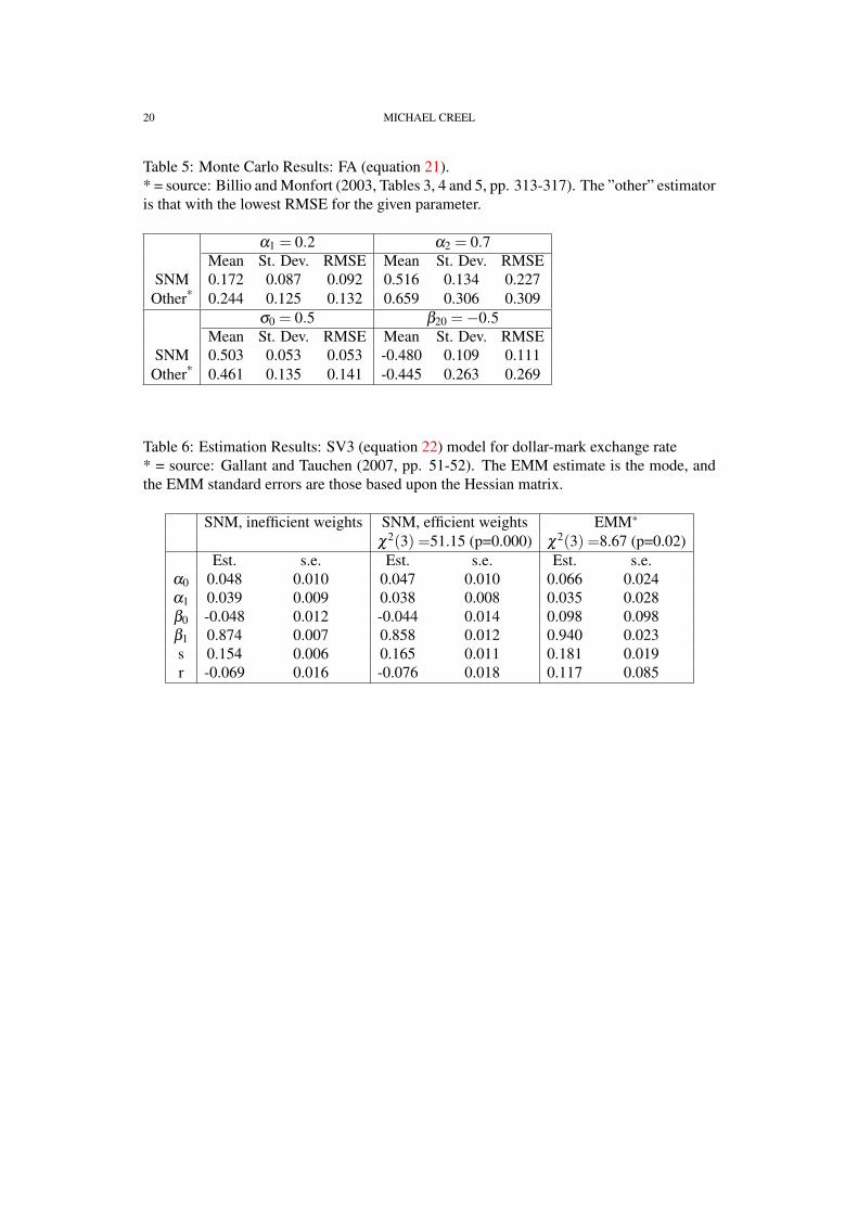
All of the 500 Monte Carlo replications obtained normal convergence. Table 5 reportsthe results, together with the lowest RMSE that Billio and Monfort obtain using severalversions of kernel-based indirect inference, indirect inference, and simulated method ofmoments (see Billio and Monfort, 2003, Table 5, page 317). For all four parameters, theSNM estimator dominates the estimators considered by Billio and Monfort in terms of low-est RMSE, though for α2 the bias of the SNM estimator is somewhat larger than one wouldlike.

3.4. Summary. This section has illustrated how the SNM estimator may be applied in theestimation of several DLV models. Moment conditions can be chosen with an eye to theinformation that they provide about specific parameters. The combination of M-estimationerror functions, compactification of the conditioning variables, and use of simulated an-nealing to find good start values lead to a numerically stable estimator that almost alwaysconverges. The SNM estimator has been applied subject to several limitations: 1) the sim-ulation length in all cases was quite short (S = 10000); 2) the bandwidth parameter (hS inequation 8) has in all cases been a naive rule-of-thumb rather than a data-based rule that canadapt to the nature of the data that a model generates; and 3) an efficient weighting matrixhas not been used.

4. APPLICATION: DOLLAR-MARK EXCHANGE RATE

To illustrate application of the SNM estimator to real data, and to offer an additionalcomparison of the SNM estimator to the EMM estimator, this section presents SNM esti-mates of the parameters of the stochastic volatility model used by Gallant and Tauchen inthe User’s Guide to the EMM software package (Gallant and Tauchen, 2007) to illustratethe EMM estimator. The data consists of 834 observations of the weekly percentage changeof the US dollar to German mark exchange rate, over the years 1975 to 1990. The data isincluded with the EMM software, and is used here without any alterations. The model used

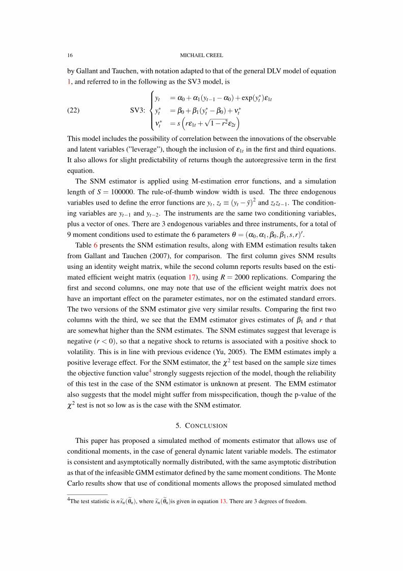
16 MICHAEL CREEL

by Gallant and Tauchen, with notation adapted to that of the general DLV model of equation1, and referred to in the following as the SV3 model, is

(22) SV3:

yt = α0 +α1(yt−1−α0)+ exp(y∗t )ε1t

y∗t = β0 +β1(y∗t −β0)+ν∗t

ν∗t = s(

rε1t +√

1− r2ε2t

)This model includes the possibility of correlation between the innovations of the observableand latent variables (”leverage”), though the inclusion of ε1t in the first and third equations.It also allows for slight predictability of returns though the autoregressive term in the firstequation.

The SNM estimator is applied using M-estimation error functions, and a simulationlength of S = 100000. The rule-of-thumb window width is used. The three endogenousvariables used to define the error functions are yt , zt ≡ (yt − y)2 and ztzt−1. The condition-ing variables are yt−1 and yt−2. The instruments are the same two conditioning variables,plus a vector of ones. There are 3 endogenous variables and three instruments, for a total of9 moment conditions used to estimate the 6 parameters θ = (α0,α1,β0,β1,s,r)′.

Table 6 presents the SNM estimation results, along with EMM estimation results takenfrom Gallant and Tauchen (2007), for comparison. The first column gives SNM resultsusing an identity weight matrix, while the second column reports results based on the esti-mated efficient weight matrix (equation 17), using R = 2000 replications. Comparing thefirst and second columns, one may note that use of the efficient weight matrix does nothave an important effect on the parameter estimates, nor on the estimated standard errors.The two versions of the SNM estimator give very similar results. Comparing the first twocolumns with the third, we see that the EMM estimator gives estimates of β1 and r thatare somewhat higher than the SNM estimates. The SNM estimates suggest that leverage isnegative (r < 0), so that a negative shock to returns is associated with a positive shock tovolatility. This is in line with previous evidence (Yu, 2005). The EMM estimates imply apositive leverage effect. For the SNM estimator, the χ2 test based on the sample size timesthe objective function value4 strongly suggests rejection of the model, though the reliabilityof this test in the case of the SNM estimator is unknown at present. The EMM estimatoralso suggests that the model might suffer from misspecification, though the p-value of theχ2 test is not so low as is the case with the SNM estimator.

5. CONCLUSION

This paper has proposed a simulated method of moments estimator that allows use ofconditional moments, in the case of general dynamic latent variable models. The estimatoris consistent and asymptotically normally distributed, with the same asymptotic distributionas that of the infeasible GMM estimator defined by the same moment conditions. The MonteCarlo results show that use of conditional moments allows the proposed simulated method

4The test statistic is n sn(θn), where sn(θn)is given in equation 13. There are 3 degrees of freedom.

ESTIMATION OF DYNAMIC LATENT VARIABLE MODELS USING SIMULATED NONPARAMETRIC MOMENTS17

of moments estimator to obtain efficiency that is very competitive with other estimationmethods.

The SNM estimator relies on the user specifying the moment conditions to use in estima-tion, as is the case with any method of moments estimator, but the rest of the process can beautomatized in software to a high degree. In the present implementation, the kernel functionis a Gaussian product kernel, and the bandwidth is chosen using a given rule that dependsonly on the number of conditioning variables and on the simulation length. One can usethe proposed Monte Carlo estimator of the efficient weight matrix that requires no tuning orpre-whitening decisions. Some of the other estimators to which the SNM estimator is com-pared in this paper require much more active decision making on the part of the modeler.An example is the newer version of the EMM estimator that uses MCMC methods, as pre-sented in Gallant and Tauchen (2007). This version of EMM requires estimation of a SNPdensity augmented by a leading parametric model to define the score generator. Selection ofthe parameterization of the score generator is complicated by the fact that it involves manyparameters. After estimation of the score generator, the model is estimated using MCMCmethods that also require judgement about proper tuning of the Markov chain. Anotherexample is the KBII estimator proposed by Billio and Monfort. Selection of the points atwhich the binding functions are evaluated is a non-trivial issue which requires judgement.The Monte Carlo results reported here suggest that the SNM estimator can give good per-formance without requiring the modeler to make any decisions other than the set of momentconditions to use.

The Monte Carlo results provided in this paper show that the SNM estimator achievesroot mean squared errors that are often better than those of alternative estimators, and arerarely worse. These results are quite acceptable as they stand, but it is anticipated that theymay be improved upon in the future, for two reasons. First, use of an estimated optimalweight matrix is likely to improve efficiency of estimation. Preliminary results suggest thatthe covariance matrix of the moment conditions can be estimated quite reliably using aMonte Carlo estimator. Future work will investigate the performance of the SNM estimatorusing an estimated optimal weight matrix. Secondly, a data-based method of choosing thesmoothing parameter could improve the fit of the kernel smoother to the true conditionalexpectations, which would likely improve the results of the SNM estimator. These are sim-ple, obvious extensions to expore. Additional topics for further research include methods toobtain a high precision fit to the conditional moments that define the estimator while usingless computational time. Possibilities include the use of sieve estimation methods insteadof kernel smoothing, use of approximate nearest neighbors, and use of high performancealgorithms for kernel smoothing, such as the improved fast Gauss transform (Yang et al.,2003). Use of an optimal bandwidth may also be helpful for this purpose, since it may bepossible to obtain the same quality of fit to φ(xt ;θ) while using a shorter simulation length.Another interesting possibility is to attempt to use optimal or approximately optimal instru-ments. Use of a local linear kernel function instead of the local constant kernel used in thispaper would automatically provide estimates of the derivatives ∂φ(xt ;θ)/∂x′t (see equation

18 MICHAEL CREEL

2) of conditional moments with respect to each of the conditioning variables, which couldbe of use in attempting to approximate optimal instruments.

A CD image that provides the current implementation of the SNM estimator with exam-ples is available on request from the author.

6. APPENDIX

Proof of Proposition 1: As n grows, Assumptions 3 and 5 let us state that

(23)(

φ(xt ;θ)− φ(xt ;θ))

j= op(1)

for j = 1,2, ...,ky. Recall that there are kykz moment conditions. Considering the differencebetween m(xt ;θ) (defined in (4)) and m(xt ;θ) (defined in (11)), focus on the qth of the kykz

elements of these vectors. Say that this element is the interaction between the jth errorfunction and the rth instrument (r = 1,2, ...,kz). Then

(m(xt ;θ)−m(xt ;θ))q = (z(xt))r

(yt − φ(xt ;θ)

)j− (z(xt))r (yt −φ(xt ;θ)) j

= (z(xt))r

(φ(xt ;θ)− φ(xt ;θ)

)j

= Op(1)op(1)

= op(1),

by Assumption 6 and equation 23. Averaging over all observations gives

(mn(θ)−mn(θ))q =1n

n

∑t=1

op(1)

= op(n−1)

Furthermore, this holds for all of the moment conditions q = 1,2, ...,kykz. Given this, theobjective function that defines the SNM estimator can be written as

sn(θ) = m′n(θ)W (τn)mn(θ)

= m′n(θ)W (τn)mn(θ)+op(n−1)

= sn(θ)+op(n−1)

Need to finish this!

ESTIMATION OF DYNAMIC LATENT VARIABLE MODELS USING SIMULATED NONPARAMETRIC MOMENTS19

TABLES

Table 1: Monte Carlo Results: CLM (equation 15). SNM-GMM is the difference betweenthe SNM and the GMM estimators.

β1 β2Mean St. Dev. Min Max Mean St. Dev. Min Max

SNM-GMM -0.001 0.004 -0.015 0.014 0.002 0.007 -0.020 0.025GMM 0.489 0.473 -0.867 2.143 0.524 0.723 -1.510 2.964

Table 2: Monte Carlo Results: SV1 (equation 18).* = source: Andersen et al. (1999, Table 2, page 72)

α =−0.736 β = 0.90 σ = 0.363Mean St. Dev. RMSE Mean St. Dev. RMSE Mean St. Dev. RMSE

SNM -0.653 0.190 0.208 0.916 0.025 0.029 0.285 0.099 0.126EMM/GMM* -0.80 0.32 0.33 0.89 0.04 0.04 0.35 0.10 0.10

Table 3: Monte Carlo Results: SV2 (equation 19).* = source: Fermanian and Salanié (2004, Table 4, page 717)** = source: Altissimo and Mele (2007, Table 1, page 48)

φ = 0.95 σb = 0.025 σε = 0.26Mean St. Dev. RMSE Mean St. Dev. RMSE Mean St. Dev. RMSE

SNM 0.973 0.031 0.038 0.023 0.002 0.003 0.131 0.093 0.158NPSML* 0.913 0.10 0.107 0.022 0.003 0.004 0.318 0.17 0.180

CD-SNE** 0.909 0.102 0.110 0.024 0.003 0.003 0.229 0.131 0.134J-SNE** 0.942 0.095 0.095 0.027 0.005 0.005 0.297 0.144 0.149

Table 4: Monte Carlo Results: AR Tobit (equation 20).* = source: Fermanian and Salanié (2004, Table 1, pg 715)

α = 0.0 β = 0.5 σ = 1.0Mean St. Dev. RMSE Mean St. Dev. RMSE Mean St. Dev. RMSE

SNM 0.102 0.117 0.155 0.411 0.109 0.140 0.700 0.130 0.327NPSML* -0.010 0.215 0.215 0.510 0.151 0.151 0.810 0.184 0.264

20 MICHAEL CREEL

Table 5: Monte Carlo Results: FA (equation 21).* = source: Billio and Monfort (2003, Tables 3, 4 and 5, pp. 313-317). The ”other” estimatoris that with the lowest RMSE for the given parameter.

α1 = 0.2 α2 = 0.7Mean St. Dev. RMSE Mean St. Dev. RMSE

SNM 0.172 0.087 0.092 0.516 0.134 0.227Other* 0.244 0.125 0.132 0.659 0.306 0.309

σ0 = 0.5 β20 =−0.5Mean St. Dev. RMSE Mean St. Dev. RMSE

SNM 0.503 0.053 0.053 -0.480 0.109 0.111Other* 0.461 0.135 0.141 -0.445 0.263 0.269

Table 6: Estimation Results: SV3 (equation 22) model for dollar-mark exchange rate* = source: Gallant and Tauchen (2007, pp. 51-52). The EMM estimate is the mode, andthe EMM standard errors are those based upon the Hessian matrix.

SNM, inefficient weights SNM, efficient weights EMM∗

χ2(3) =51.15 (p=0.000) χ2(3) =8.67 (p=0.02)Est. s.e. Est. s.e. Est. s.e.

α0 0.048 0.010 0.047 0.010 0.066 0.024α1 0.039 0.009 0.038 0.008 0.035 0.028β0 -0.048 0.012 -0.044 0.014 0.098 0.098β1 0.874 0.007 0.858 0.012 0.940 0.023s 0.154 0.006 0.165 0.011 0.181 0.019r -0.069 0.016 -0.076 0.018 0.117 0.085

ESTIMATION OF DYNAMIC LATENT VARIABLE MODELS USING SIMULATED NONPARAMETRIC MOMENTS21

REFERENCES

[1] Altissimo, F. and A. Mele (2007) Simulated Nonparametric Estimation of Dynamic Models, workingpaper.

[2] Andersen, T. and B. Sorensen (1996) GMM estimation of a stochastic volatility model: A Monte Carlostudy, Journal of Business & Economic Statistics, 14, 328-352.

[3] Andersen, T., H.-J. Chung and B. Sorensen (1999) Efficient method of moments estimation of a stochasticvolatility model: A Monte Carlo study, Journal of Econometrics, 91, 61-87.

[4] Bierens, H. (1987) Kernel estimators of regression functions, in Advances in Econometrics, Vol 1 (ed. T.Bewley), Cambridge University Press, 99-144.

[5] Billio, Monica and Alain Monfort (2003) Kernel-based indirect inference, Journal of Financial Econo-metrics, 1, 297-326.

[6] Carrasco, M., M. Chernov, J.-P. Florens and E. Ghysels (2007) Efficient estimation of general dynamicmodels with a continuum of moment conditions, Journal of Econometrics 140, 529-573.

[7] Chernozhukov, V. and H. Hong (2003) An MCMC approach to classical estimation, Journal of Economet-rics, 115, 293-346.

[8] Creel, M. (2005) User-friendly parallel computations with econometric examples, Computational Eco-nomics, 26, 107-128.

[9] Creel, M. (2007) I ran four million probits last night: HPC clustering with ParallelKnoppix, Journal ofApplied Econometrics, 22, 215-223.

[10] Fermanian, J.-D. and B. Salanié (2004) A nonparametric simulated maximum likelihood estimationmethod, Econometric Theory, 20, 701-734.

[11] Fiorentini, Gabriele, Enrique Sentana, and Neil Shephard (2004) Likelihood-based estimation of latentgeneralized ARCH structures, Econometrica, 72, 1481-1517.

[12] Florens, J.P., M. Mouchart and J. M. Rolin (1993) Noncausality and marginalization of Markov processes,Econometric Theory, 9, 241-262.

[13] Gallant, A.R. (1987) Nonlinear Statistical Models, John Wiley & Sons.[14] Gallant, A. R., and D. Nychka (1987) Seminonparametric maximum likelihood estimation, Econometrica,

55, 363–390.[15] Gallant, A. R. and G. Tauchen (1996) Which moments to match? Econometric Theory 12, 657– 681.[16] Gallant, A. Ronald, and George Tauchen (1999) The relative efficiency of method of moments estimators,

Journal of Econometrics, 92, 149-172.[17] Gallant, A. Ronald, and George Tauchen (2002) Simulated score methods and indirect inference for

continuous-time models, Chapter in preparation for the Handbook of Financial Econometrics.[18] Gallant, A. Ronald, and George Tauchen (2004) EMM: A program for efficient method of moments

estimation: User’s Guide Version 1.7, http://econ.duke.edu/webfiles/get/emm/ver17/guide/.

[19] Gallant, A. Ronald, and George Tauchen (2007) EMM: A program for efficient method of moments esti-mation: User’s Guide Version 2.5, http://econ.duke.edu/webfiles/arg/emm/emm.tar.

[20] Goffe, W.L., G. D. Ferrier and J. Rogers (1994) Global optimization of statistical functions with simulatedannealing, Journal of Econometrics, 60, 65-99.

[21] Gouriéroux, C. and A. Monfort (1996) Simulation-based econometric methods, Oxford University Press.[22] Gouriéroux, C., A. Monfort, and E. Renault (1993), Indirect inference, Journal of Applied Econometrics,

8, S85–S118.[23] Hajivassiliou, V. and D. McFadden (1998) The method of simulated scores for the estimation of limited-

dependent variable models, Econometrica, 66, 863–896.[24] Härdle, W. (1991) Applied Nonparametric Regression, Cambridge University Press.[25] Hansen, L., J. Heaton and A. Yaron (1996) Finite-sample properties of some alternative GMM estimators,

Journal of Business & Economic Statistics, 14, 262-280.

22 MICHAEL CREEL

[26] Huber, P. (1964) Robust estimation of a location parameter, Annal of Mathematical Statistics, 35, 73-101.[27] Kristensen, D. and Y. Shin (2006) Estimation of dynamic models with nonparametric simulated max-

imum likelihood, working paper, http://www.columbia.edu/~dk2313/workingpapers/wp_files/fo-smle-18-01-06.pdf.

[28] Laroque, G. and B. Salanié (1993) Simulation-based estimation of models with lagged latent variables,Journal of Applied Econometrics, 8, S119–S133.

[29] Lee, L.F. (1995) Asymptotic bias in simulated maximum likelihood estimation of discrete choice models,Econometric Theory, 11, 437– 483.

[30] Li, Q. and J. Racine (2007), Nonparametric econometrics, Princeton University Press.[31] Lu, Z. and P. Cheng (1997) Distribution-free strong consistency for nonparametric kernel regression in-

volving nonlinear time series, Journal of Statistical Planning and Inference, 65, 67-86.[32] McFadden, D. (1989) A method of simulated moments for estimation of discrete response models without

numerical integration, Econometrica, 57, 995–1026.[33] Michaelides, A. and Ng, S. (2000) Estimating the rational expectations model of speculative storage: A

Monte Carlo comparison of three simulation estimators, Journal of Econometrics, 96, 231-66.[34] Newey, W.K. and K.D. West (1987) A simple, positive semi-definite, heteroskedasticity and autocorrela-

tion consistent covariance matrix, Econometrica, 55, 703-08.[35] Pakes, A. D. Pollard (1989), Simulation and the asymptotics of optimization estimators, Econometrica,

57, 1027–1057.[36] Racine, Jeff (2002) Parallel distributed kernel estimation, Computational Statistics & Data Analysis, 40,

293-302.[37] Robinson, P. (1983) Nonparametric estimators for time series, Journal of Time Series Analysis, 4, 185-207.[38] Smith, A. (1993) Estimating nonlinear time series models using simulated vector autoregressions, Journal

of Applied Econometrics, 8, S63–S84.[39] Tauchen, George (1997) New minimum chi-square methods in empirical finance, in Advances in Econo-

metrics, Seventh World Congress, eds. D. Kreps, and K. Wallis, Cambridge UK: Cambridge UniversityPress, 279–317.

[40] Windmeijer, F. (2005) A finite sample correction for the variance of linear efficient two-step GMM esti-mators, Journal of Econometrics, 126, 25-51.

[41] Yang, C., R. Duraiswami, N. Gumerov and L. Davis (2003) Improved fast Gauss transform and efficientkernel density estimation, Ninth IEEE International Conference on Computer Vision (ICCV’03), 1, 464-471.

[42] Yu, J. (2005) On leverage in a stochastic volatility model, Journal of Econometrics, 127, 165-178.