Estimation of impedance and susceptance parameters of a 3-phase cable system using PMU dataCitation for published version (APA):Singh, R. S., van den Brom, H., Babaev, S., Cobben, S., & Cuk, V. (2019). Estimation of impedance andsusceptance parameters of a 3-phase cable system using PMU data. Energies, 12(23), [4573].https://doi.org/10.3390/en12234573

DOI:10.3390/en12234573

Document status and date:Published: 30/11/2019

Document Version:Publisher’s PDF, also known as Version of Record (includes final page, issue and volume numbers)

Please check the document version of this publication:

• A submitted manuscript is the version of the article upon submission and before peer-review. There can beimportant differences between the submitted version and the official published version of record. Peopleinterested in the research are advised to contact the author for the final version of the publication, or visit theDOI to the publisher's website.• The final author version and the galley proof are versions of the publication after peer review.• The final published version features the final layout of the paper including the volume, issue and pagenumbers.Link to publication

General rightsCopyright and moral rights for the publications made accessible in the public portal are retained by the authors and/or other copyright ownersand it is a condition of accessing publications that users recognise and abide by the legal requirements associated with these rights.

• Users may download and print one copy of any publication from the public portal for the purpose of private study or research. • You may not further distribute the material or use it for any profit-making activity or commercial gain • You may freely distribute the URL identifying the publication in the public portal.

If the publication is distributed under the terms of Article 25fa of the Dutch Copyright Act, indicated by the “Taverne” license above, pleasefollow below link for the End User Agreement:www.tue.nl/taverne

Take down policyIf you believe that this document breaches copyright please contact us at:openaccess@tue.nlproviding details and we will investigate your claim.

Download date: 30. Jan. 2022

energies

Article

Estimation of Impedance and Susceptance Parametersof a 3-Phase Cable System Using PMU Data

Ravi Shankar Singh 1,∗ , Helko van den Brom 2 , Stanislav Babaev 1 and Sjef Cobben 1

and Vladimir Cuk 1

1 Electrical Energy Systems Group, Eindhoven University of Technology, 5600 MB Eindhoven,The Netherlands; s.babaev@tue.nl (S.B.); j.f.g.cobben@tue.nl (S.C.); V.Cuk@tue.nl (V.C.)

2 VSL, 2629 JA Delft, The Netherlands; hvdbrom@vsl.nl* Correspondence: r.singh1@tue.nl

Received: 29 September 2019; Accepted: 29 October 2019; Published: 30 November 2019

Abstract: This paper proposes a new regression-based method to estimate resistance, reactance, andsusceptance parameters of a 3-phase cable segment using phasor measurement unit (PMU) data. Thenovelty of this method is that it gives accurate parameter estimates in the presence of unknown biaserrors in the measurements. Bias errors are fixed errors present in the measurement equipment andhave been neglected in previous such attempts of estimating parameters of a 3-phase line or cablesegment. In power system networks, the sensors used for current and voltage measurements haveinherent magnitude and phase errors whose measurements need to be corrected using calibratedcorrection coefficients. Neglecting or using wrong error correction coefficients causes fixed bias errorsin the measured current and voltage signals. Measured current and voltage signals at different timeinstances are the variables in the regression model used to estimate the cable parameters. Thus,the bias errors in the sensors become fixed errors in the variables. This error in variables leads toinaccuracy in the estimated parameters. To avoid this, the proposed method uses a new regressionmodel using extra parameters which facilitate the modeling of present but unknown bias errors in themeasurement system. These added parameters account for the errors present in the non- or wronglycalibrated sensors. Apart from the measurement bias, random measurement errors also contribute tothe total uncertainty of the estimated parameters. This paper also presents and compares methodsto estimate the total uncertainty in the estimated parameters caused by the bias and random errorspresent in the measurement system. Results from simulation-based and laboratory experiments arepresented to show the efficacy of the proposed method. A discussion about analyzing the obtainedresults is also presented.

Keywords: distribution grid monitoring; cable temperature estimation; cable parameter estimation;PMU application in distribution grid; metrology in smart grids

1. Introduction

Accurate estimates of line parameters are useful in improving the performance of power systemmonitoring and protection applications like accurate relay settings and fault location [1]. Distancerelays have reach zone settings based on the known positive sequence impedance of the protected linesegment. High accuracy impedance estimates of the protected line would assist in a more accuratesetting of the impedance in the distance relay which protects the line. It is known that accurate pre-faultline impedance and knowledge about impedance of loads on the line could be utilized to calculatethe location of the faults more precisely [2]. A novel idea of utilizing real-time resistance estimates tomonitor the temperature of an overhead line or a cable and facilitate dynamic line rating (DLR) wasfirst mentioned in [3]. It was presented that the relationship between the conductor resistance and

Energies 2019, 12, 4573; doi:10.3390/en12234573 www.mdpi.com/journal/energies

Energies 2019, 12, 4573 2 of 22

temperature could be utilized to estimate the real-time temperature of the conductor. The estimatedtemperature could then be utilized to access the thermal state and set flexible loading levels of powerlines in real-time. For cables, parameters (resistance (R), reactance (X) and susceptance (B)) have beencalculated using the available information and assumptions on the physical attributes of the cablesegment like length, conductor dimension, ambient soil temperature, and moisture content. However,these methods are static in nature as the used specifications are considered constant for long periods,while the cable resistance could change based on ambient temperature and loading levels. Monitoringof cable temperature in real time and implementation of DLR based on the cable temperature wouldrequire more reliable and frequent estimates of the cable parameters (especially resistance).

To facilitate the first step of temperature based DLR (monitoring of cable conductor temperature),this paper proposes a method to estimate the resistance of 3-phase cable system utilizing real-timephasor measurement unit (PMU) measurements. Other parameters like cable reactance andsusceptance are also estimated alongside. When compared to the previous methods, the proposedmethod is suitable for a 3-phase system and gives more accurate results in the presence of errors inthe measurement equipment. The proposed method also facilitates a more reliable estimation of theuncertainty in the achieved results.

In the recent past, methods have been presented that utilize PMU data to estimate theoverhead-line parameters [4–8]. These methods estimate line parameters utilizing voltage and currentphasors at both ends of the line segment and could give frequent parameter estimates. The authorsin [5] presented an ordinary least squares (OLS)-based regression method to estimate the impedanceparameters of an overhead transmission line. The effect of random errors in the phasor measurementswere analyzed. However, the effect of bias error in the measurements was not considered. The biaserror comes from the magnitude and phase errors in the measurement sensors. For medium voltage(MV) and high voltage (HV) networks, these sensors are current and voltage transformers (CTs andVTs, respectively) which transform the current and voltage signals into low amplitude signals beforefeeding to the PMUs. As is shown later, the bias errors in the measurements contribute to the total errorin the parameter estimates. A novel method for estimating the parameters of an overhead transmissionline was described in [6], where the bias errors are accounted for while estimating the parameters.However, to estimate the correct bias correction coefficients, the authors use an assumption that theresistance varies linearly over a short period relative to the time constant of the conductor. Moreover,the estimation algorithm is developed and tested only for single phase lines. Three-phase lines havemutual coupling elements and estimating the parameters has challenges in terms of modeling andsignal excitation requirements. Hence, it was noted in [7] that the application of such an algorithmfor 3-phase lines would require more complex models. Also, no tests were done to demonstrate theperformance of the method for actual measurements. A three-phase parameter estimation problemusing a robust parameter estimation is discussed in [8]. The paper also describes the importance ofpower system operating conditions characterized by characteristics like correlation, dependence andlevel of unbalance between the three-phase voltage and current signals on the overall uncertainty of theestimates. A field test of a fully transposed overhead HV transmission line was done to demonstratethe algorithm. However, for their field test, the bias correction coefficients for both ends of the VTswere already known. Thus, none of the previous methods are suitable to estimate parameters of a3-phase cable system in the presence of both random and bias errors in the measurement chain.

In previous works [5,7], the metrics for the evaluation of the results were based on the knowledgeof the actual parameter values. However, in the real application cases, reference values are either notavailable or are not reliable enough to the desired level. This makes this type of validation processless suitable for application using real-field data, since the reference parameters might have changeddepending on the ambient environmental and power system operating conditions. The authors in [8]also specified that there was a discrepancy between parameters they estimated and the reference valueof those. The highest difference observed was of 13% in the estimated resistance. In the absence of a

Energies 2019, 12, 4573 3 of 22

reliable reference, this could not be explained. Hence, it is very important to have a reliable measure ofuncertainty associated with the estimated parameters.

This paper presents solutions to both concerns stated above. It presents a method which is capableof providing accurate parameter estimates even in the presence of unknown bias errors in the sensors.It also presents and compares different methods to calculate the total uncertainty associated withthe parameter estimates. It is mentioned in [8] that factors like unbalanced loading levels and someindependence in the power flow in the 3 phases are the necessary conditions for convergence of thealgorithm. The absence of unbalanced and independent power flow could cause the OLS problem tobecome ill-conditioned. However, the effects of such an ill-conditioned OLS problem on the uncertaintyof parameter results was not discussed in detail. This paper also presents a discussion on the conditionof the measurement matrices and its effect on the results.

The remainder of the paper is arranged as follows: Section 2 discusses the core of the previousline parameter estimation methods, and their drawbacks are discussed. Section 3 presents the newparameter estimation algorithm. Section 4 presents various methods to calculate the uncertainty ofthe estimated parameters. Section 5 presents the results from the simulation and laboratory testsand evaluates the methods presented for calculation of the uncertainty in the estimated parameters.Discussion about the general guidelines for applying the proposed method is presented in Section 6,and conclusions are drawn in Section 7.

2. Existing Parameter Estimation Methods and Drawbacks

To estimate the parameters of a 3-phase line-segment, two different methods are presented in [5,8].However, they use the same regression model with different objective functions. A robust objectivefunction was chosen in [8] to get better estimates in the presence of outliers in the measurements. Inthis paper, both the previous methods are considered to give similar results in the absence of outliers.Hence, both are treated as the same and referred to as the existing method. Results obtained byOLS-based objective function as used in [5] are used for comparison with the proposed method. Thissection presents and discusses the drawbacks of the regression model used in the existing method.

A 3-phase cable segment is represented by a nominal Pi model. Based on the nominal Pi modelshown in Figure 1, relationships between the measured current and voltage at the two ends can bedescribed using Equations (1) and (2).

ISabc − IR

abc =Babc

2

(VS

abc + VRabc

), (1)

VSabc −VR

abc = Zabc

(Babc

2VR

abc + IRabc

), (2)

where Zabc and Babc are 3× 3 matrices of unknown cable parameters with self components as diagonalelements and mutual components as off-diagonal elements. Superscript S/R denotes the sendingand receiving end of the cable, and subscripts ABC denote the 3-phases system. Using phasors givenby PMUs, voltage and current signals are represented as complex numbers in Cartesian coordinates.Equations (1) and (2) are separated into real and imaginary terms, giving a set of 12 equations. Theseequations are then solved in linear least-squares sense to estimate the unknown Rabc, Xabc, and Babcparameters. The set of linear equations with p parameters can be written as:

yi = h1iθ1 + h2iθ2 + ... + hpiθp + εi, (3)

where, according to Equations (1) and (2), yi is made up of real or imaginary parts of ∆IABC or ∆VABC,hij is real or imaginary IABC or VABC, and θj are the cable parameters to be estimated. εi is the errorterm calculated as the difference between the measured quantity and the result of the linear equationformed by parameters and independent variables. For p parameters and n sets of observations, thewhole system of linear equations is represented in matrix form as:

Energies 2019, 12, 4573 4 of 22

Y[12n×1] = H[12n×p]θ[p×1] + E[12n×1], (4)

where Y is the measurement vector and θ is the parameters vector. H is the relation matrix formed ofvariables which are real or imaginary components of the measured voltage and current phasors.

VS VR

IL

jB/2 jB/2

IS IR

R+jX

Figure 1. Nominal Pi model for a medium length medium voltage line.

The estimates for parameter θ are given by the equation:

θ =covariance(Y, H)

variance(H). (5)

In matrix form, the analytical solution could be found out by solving the OLS problem minθ ||Y− Hθ||2.The solution is given as:

θ = (HT H)−1HTY. (6)

The analysis of the estimated parameters and residuals is an important as well as challenging part ofvalidation of the results. Given that the system being measured is modeled correctly using Equation (3),the parameters obtained using OLS-based regression are true and unbiased only when the residualsadhere to properties:

(a) Zero mean error: Residuals have a distribution with zero mean such that E[εi] = 0;(b) No heteroscedasticity: The residuals have a constant variance. Each residual εi has the same

finite variance σ2;(c) Independent variables: There is no correlation between the residuals and the independent

variable, E[εi|hj1, hj1, ..., hjn] = 0;(d) Normality: The error vector is normally distributed.

Assumptions a–d can be summarized in matrix notation as:

ε = N(0, σ2 I). (7)

In field measurements, each of these assumptions might not hold true. Apart from the randommeasurement errors, field CTs and VTs have a steady bias error in their measurement due to theinherent magnitude and phase errors of different magnitudes. As shown in Equation (3), elementsof the matrix H and vector Y are real and imaginary parts of measured current and voltage phasors.The presence of any magnitude and phase errors in the measurement chain would cause a fixed biaserror in those elements. Use of the same regression model as in the existing method will result inresiduals which will not have a normal distribution. The expected value of residuals might also benon-zero. This indicates a mismatch between the system model used in the regression model andthe measurements acquired from the system. Thus, the estimated model parameters will differ fromthe actual parameters. In such cases of measurements with bias errors, the calculated uncertainty ofthe parameters would be wrong. This is because the OLS problem formulation assumes that all ofthe errors are present in the vector Y and have a normal distribution. In the current case of the OLSproblem, the variables (hij) are also made up of measured quantities, like current and voltage phasors.These variables, apart from having random noise errors, also have fixed bias errors which do not have

Energies 2019, 12, 4573 5 of 22

a normal distribution. Thus, the existing method does not address the effect of bias errors on thequality of the parameter estimates.

Section 3 presents the proposed method, which gives more accurate results in the presence ofbias and random errors in the measured variables. After that, Section 4 presents different methodsto estimate the uncertainty in the estimated results in the presence of bias and random errors inthe variables.

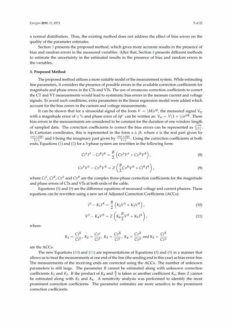
3. Proposed Method

The proposed method utilizes a more suitable model of the measurement system. While estimatingline parameters, it considers the presence of possible errors in the available correction coefficients formagnitude and phase errors in the CTs and VTs. The use of erroneous correction coefficients to correctthe CT and VT measurements would lead to systematic bias errors in the measure current and voltagesignals. To avoid such conditions, extra parameters in the linear regression model were added whichaccount for the bias errors in the current and voltage measurements.

It can be shown that for a sinusoidal signal of the form V = |M|ejφ, the measured signal Vm

with a magnitude error of γ % and phase error of δφ can be written as: Vm = V(1 + γ)ejδφ. Thesebias errors in the measurements are considered to be constant for the duration of one window lengthof sampled data. The correction coefficients to correct the bias errors can be represented as e±jδφ

1+γ .In Cartesian coordinates, this is represented in the form a ± jb, where a is the real part given bycos(±jδφ)

1+γ and b being the imaginary part given by sin(±jδφ)1+γ . Using the correction coefficients at both

ends, Equations (1) and (2) for a 3-phase system are rewritten in the following form:

CiS IS − CiR IR =B2

(CvSVS + CvRVR

), (8)

CvSVS − CvRVR = Z(

B2

CvRVR + CiR IR)

, (9)

where CiS, CiR, CvS and CvR are the complex three-phase correction coefficients for the magnitudeand phase errors of CTs and VTs at both ends of the cable.

Equations (8) and (9) are the difference equations of measured voltage and current phasors. Theseequations can be rewritten using a new set of Adjusted Correction Coefficients (ACCs):

IS − K1 IR =B2

(K2VS + K3VR

), (10)

VS − K4VR = Z(

K4B2

VR + K5 IR)

, (11)

where:

K1 =CiR

CiS , K2 =Cvs

CiS , K3 =CvR

CiS , K4 =CvR

CvS and K5 =CiR

CvS

are the ACCs.The new Equations (10) and (11) are representations of Equations (8) and (9) in a manner that

allows us to treat the measurements at one end of the line (the sending end in this case) as bias-error-free.The measurements of the receiving ends are corrected using the ACCs. The number of unknownparameters is still large. The parameter B cannot be estimated along with unknown correctioncoefficients K2 and K3. If the product of K4 and B

2 is taken as another coefficient K6, then Z cannotbe estimated along with K5 and K6. A sensitivity analysis was performed to identify the mostprominent correction coefficients. The parameter estimates are more sensitive to the prominentcorrection coefficients.

Energies 2019, 12, 4573 6 of 22

For this analysis, a 10 km long MV cable (20 kV) was simulated. The maximum magnitudeand phase error in CTs and VTs was limited to 1% in magnitude and 1 in phase. Hence, the CTand VT magnitude errors were varied as per a random uniform distribution in the range between0% and 1%. Similarly the phase angle errors of the CTs and VTs were varied between 0 anf 1. Thecoefficients K1–K5 were calculated based on these magnitudes and phase errors and were substitutedin Equations (10) and (11) to calculate the deviation in B, Z parameters. The results are presented inFigures 2 and 3. For the simulated system, it was observed that the error in B varied within 1 % due tocoefficients K2 and K3 individually. At the same time, the error in B is highly sensitive to K1. A similaranalysis showed that the R and X are sensitive to K4.and It was observed that the R and X estimateswere little affected by the errors in K5 and K6. Hence, only ACCs K1 and K4 were used into the systemof linear equations, and B

2 was used instead of K4 × B2 .

IS = K1 IR +B2

(VS + VR

)(12)

VS = K4VR + Z(

B2

VR + IR)

(13)

0.0200.99

5

Im(K1)

0

10

Re(K1)

Err

or

in B

(%

)

1

15

20

-0.021.01

0.0200.99

0.2

Im(K2)

0

Re(K2)

Err

or

in B

(%

)

1

0.4

0.6

-0.021.01

0.0200.99

0.2

Im(K3)

0

Re(K3)

Err

or

in B

(%

)

1

0.4

0.6

-0.021.01

Figure 2. Sensitivity of B with respect to coefficients K1, K2, and K3.

0.0200.99

Im(K4)

0

50

Re(K4)

Err

or

in R

(%

)

1

100

-0.021.01

0.0200.99

20

Im(K4)

0

Re(K4)

Err

or

in X

(%

)

1

40

60

-0.021.01

0.0200.99

Im(K5)

0

2

Re(K5)

Err

or

in R

(%

)

1

4

-0.021.01

0.0200.99

Im(K5)

0

1

Re(K5)

Err

or

in X

(%

)

1

2

-0.021.01

0.01650.2451.0086

0.25

Im(K6)

0.016

Re(K6)

Err

or

in R

(%

)

1.0088

0.255

0.26

0.01551.009

0.01650.211.0086

Im(K6)

0.016

0.22

Re(K6)

Err

or

in X

(%

)

1.0088

0.23

0.01551.009

Figure 3. Sensitivity of R and X with respect to coefficients K4, K5, and K6.

Equations (12) and (13) represent the updated model utilized by the proposed method to estimatethe cable parameters while minimizing the effect of inherent bias in the measured current and voltagesignals. These equations can be written as two separate equations for real and imaginary parts. Thiswas done for all the three phases resulting in twelve equations. Now, the parameter estimation processwas divided in two parts. All the measured data were arranged according to the six equations from

Energies 2019, 12, 4573 7 of 22

Equation (12), forming an overdetermined system of linear equations. Parameters K1 and B for allphases were estimated using the analytical solution given by Equation (6). The estimated B parameterswere substituted in Equation (13) to estimate resistance (R) and reactance (X) parameters.

After estimation of the parameters, total uncertainty in the estimated values was quantifiedby confidence interval (CI) associated with each parameter. The next section presents the methodsto estimate total uncertainty in the parameter estimates caused by random and bias errors in themeasurements of the variables.

4. Estimation of Uncertainty

The accuracy of a parameter estimate is a qualitative characteristic which is made up ofcomponents trueness and precision. Quantitative estimates of trueness and precision are givenby expected bias and standard deviation, respectively [9]. The guide to the expression of uncertaintyin measurement (GUM) specifies ways of evaluating the uncertainty of a measurement. Type Auncertainty evaluation is derived by statistical methods on a series of observations whereas TypeB evaluation is based on the specifications given by the equipment manufacturers or calibrationreports [10]. However, the system model used to estimate the cable parameters falls under the categoryof the multivariate multistage measurement model described in GUM [11]. The model specifies themanner in which the parameters are estimated using various input quantities. The standard deviationof OLS parameters is given by the diagonal vector of the covariance of the parameters. This fallsunder the type A uncertainty evaluation. However, it can be shown that this estimate of uncertaintycould be misleading in cases where the residuals do not adhere to the assumptions summarized byEquation (7). This could be caused by an inaccurate measurement model or some bias errors in themeasured variables leading to a systematic bias in the parameter estimates. Hence, to get a moreaccurate representation of uncertainty in the solution of the OLS problem, estimating the componentof systematic bias is also important. Hence, combining the bias and standard deviation error wouldgive us the total uncertainty associated with the estimated parameters.

The fixed bias error component in the parameters was evaluated using the knowledge of thebias errors present in each of the equipment. Measurement bias errors of each individual piece ofequipment could be evaluated based on the specifications given by the equipment manufacturers. Asper GUM, this is categorized as Type B evaluation of uncertainty. The error in parameter estimatesdue to the bias in the variables can be minimized by the use of correction coefficients if available.Possible errors in the correction coefficients were modeled in the system model using the ACCs K1-K5.However, in the formulation of the proposed method, correction coefficients K2, K3 K5 were ignoredand assumed to be 1. The product of K4 and B

2 was considered to be B2 . The error in the estimated

parameters caused by these assumptions was calculated using Monte Carlo-based simulations.The combined uncertainty of the parameters estimates constitutes the uncertainty caused due

to random errors in the measurements and the bias due to the assumptions made on the correctioncoefficients K2, K3, K5, and K6. Separate uncertainties for both random and bias errors were estimatedand combined to get a combined CI. Sections 4.1–4.3 present the three methods evaluated to estimatethe uncertainty in the parameters due to random errors in PMU estimates. Estimation of the bias inparameter estimates caused by the bias errors present in the variables is shown in Section 4.4.

It was shown in [12] that for a sinusoidal current or voltage signal X sampled consistent withthe Nyquist rate and containing white noise, the expected error in computed phasor (E[X]) by a fullcycle discrete Fourier transform (DFT) is zero. Hence, the CTs and VTs are a source of fixed bias errorswhere as the PMUs are the source of random errors in the voltage and current variables.

4.1. Effect of Random Errors: Standard Deviation-Based Uncertainty (Method 1)

Given that the assumptions a− d hold true, the covariance matrix of the parameter estimates isgiven by [13]:

cov(θ) = (HT H)−1σ2, (14)

Energies 2019, 12, 4573 8 of 22

where σ2 is the unbiased estimate of the variance of the residuals. The standard deviations in theparameters are calculated by taking the square root of the diagonal elements of the covariance matrix.A coverage factor of 3 was multiplied to get the expanded standard deviation (α).

α = 3×√

diag(cov(θ)) (15)

Method 1 gives the deviation in parameters caused by random noise in the measurements basedon the assumed properties of the OLS system. The system assumes that the errors are in the Y vectoronly. Sections 4.2 and 4.3 present two methods which calculate the sensitivity of the OLS solutionsdue to the random errors in the variables of the H matrix and Y vector.

4.2. Effect of Random Errors: Norm-Wise Boundary of Uncertainty (Method 2)

Due to the presence of random errors, the relationship matrix H and the vector Y are perturbedfrom their true values. Hence, for given H ∈ R(m ≥ n) and H + ∆H, The OLS problem:

minθ ||Y− Hθ||2, r = Y− Hθ (16)

in the presence of errors in measurements is transformed into:

minθ1 ||(Y + ∆Y)− (H + ∆H)θ1||2, s = Y + ∆Y− (H + ∆H)θ1, (17)

where s and r are the residuals of the OLS solution with and without the errors in variables. H + ∆Hand Y + ∆Y are made up of measured variables with errors and are renamed Hm and Ym, respectively.Backward error (∆H) is defined as the error in measured variables used in the OLS problem. Thepresence of backward error in the variables gives rise to the error in the parameter estimates whichis called the forward error (θ − θ1). Sensitivity of the OLS solution due to errors in variables wasinvestigated in [14,15]. Both component-wise and norm-wise bounds of the forward error couldbe derived.

Considering the OLS problem shown in Equation (17), Method 2 gives the uncertainty α as theratio of the euclidean norm of the expected maximum deviation and the estimated parameter vectors.It is shown in [14] that for a perturbation error η and σ1 and σn as the biggest and smallest eigenvaluesof the matrix Hm, if:

η = max

||∆H||2||Hm||2

,||∆Y||2||Ym||2

<

σn

σ1

and

sin(φ) =s

||Ym||26= 1

are satisfied, then the ratio of norms of the maximum deviation and estimated parameter vectors aregiven by:

α :=||θ1 − θ||2||θ1||2

≤ η

2κ

cos(φ)+ tan(φ)κ2

, (18)

where κ is the condition number of matrix Hm. For a given rectangular matrix H, the condition numberis defined as:

κ(H) = ||H||2||H+||2, (19)

where H+ is the pseudo-inverse of the matrix H and ||H||2 denotes the Frobenius norm of thematrix. Thus, α is the norm-wise boundary of maximum uncertainty caused by the random errors in

Energies 2019, 12, 4573 9 of 22

measurement. For small values of residuals, the maximum uncertainty is twice the condition numberof the matrix Hm.

4.3. Effect of Random Errors: Component-Wise Boundary of Uncertainty (Method 3)

Method 2 presented the norm-wise boundary of uncertainty in parameter estimates. Method 3calculates the component-wise boundary for the OLS problem shown by Equation (17). Let E and f bean arbitrary matrix and vector such that:

|∆H| ≤ ηE and |∆Y| ≤ η f .

The absolute values and inequalities between the matrices and vectors are held component-wise.However, the measured matrix Hm has different rows made up of different measurements of differentscales, and the total backward error was computed for each row rather than for each component. Fore = [1, 1, ...1]T , the matrix E and vector f can be formulated as:

E = |Hm|eeT and f = ||Y||1e.

By doing so, the errors in the ith row of Hm are measured as the L1 norm of that row.Using Equations (16) and (17), and the assumptions binding ∆H and E, it was shown in [15] that

the maximum deviation (α) in each element of the solution of the OLS problem can be calculated as:

α := |θ1 − θ| ≤ η(|H+m |( f + E|θ1 + |(HT

m Hm)−1|ET |s|), (20)

where |θ1 − θ| is the maximum deviation given for each individual parameters caused by randomerrors in measurement.

Sections 4.1–4.3 presented methods to calculate the deviation in parameter estimates caused bythe random errors in the variables. Section 4.4 presents the method to calculate the deviation causeddue to the bias in the measured variables.

4.4. Effect of Bias Errors

Although the new proposed method includes the most sensitive ACCs K1 and K4 to model thebias errors in the measurements, other coefficients K2, K3, and K5 were for the sake of simplicityignored and hence assumed to be 1. The factor of K4 × B

2 was kept as B2 . This would cause deviations

in the parameters estimates. This subsection presents a Monte Carlo-based method to estimate thedeviation due to the error in the measurement model caused by the assumptions made on of K2, K3,K5, and K6 correction coefficients.

Equations (10) and (11) were expanded, and the components were written in the complex form.The real and imaginary parts of the equation were separated as done earlier. The magnitude and phaseerrors were varied in the range of ±50% from their last calibrated values. Matrix Hi and vector Yi wereevaluated for all possible values of coefficients K2, K3, and K5. For each set of Hi and Yi, parametersθi are calculated. The maximum deviation (β) in the parameters due to bias errors in the variables isquantified by:

β ≤ max

(||θi − θ1||2)||θ1||2

, (21)

for the norm-based analysis and:

β ≤ max

(|θi − θ1|)|θ1|

, (22)

for the component based analysis.Sections 4.1–4.4 presented methods to calculate uncertainties due to random and bias errors in

the measurements. The total uncertainty for the parameter estimates was calculated combining the

Energies 2019, 12, 4573 10 of 22

uncertainties due to random and bias errors in the measured variables. The total uncertainty, denotedby a CI in the parameters, is given by:

CI ≤√

α2 + β2. (23)

Sections 3 and 4 presented the proposed method to estimate the cable parameters accurately in thepresence of random and bias errors in the measurement system and then to calculate the uncertaintyassociated with the estimation results. The complete process is summarized using a flowchart presentedin Figure 4. Model initialization is done at the beginning to select the prominent parameters of theregression model. After initialization, the method can be run in loop to give continuous estimatesof the parameters. Section 5 presents the results obtained using the proposed method along withcomparisons with the existing method.

Start

Separate Re and Im parts

Make system of linear equations (12) and (13)

Select additional parameters modelling bias

Solve (12) for B and K1

Balanced Power-flow and Trefoil?

Include Susceptance (B) parameter

Ignore Susceptance (B) parameter

Acquire Multiple Voltage and Current Phasors

Solve (13) for R, X and K4

Long cable forcapacitance?

Include mutual parameters

Ignore mutual parameters

Calculate Total Uncertainty due to random and bias errors (25)

Residuals

ε=N(0,σ I)?

Initialize the Cable and Measurement Model

No

Yes

Yes

Yes

No

No

Ch

eck

for

err

ors

in

th

e m

od

el

More Estimates?

End

Loop for Continuous Estimation

2

No

Yes

Figure 4. Flowchart summarizing the process of accurate parameter estimation of a cable segment.

5. Results and Comparison

First, both the existing and the proposed methods were tested using simulation tests. A 20 kV,10 km cable was simulated. The exact values of the parameters of simulated 3-phase cables were known.

Energies 2019, 12, 4573 11 of 22

The obtained results were evaluated based on the analysis of the residuals of the OLS problem shown inEquation (4). If the residual vector seemed to satisfactorily pass the tests to check the assumptions a− d,then the uncertainty of the parameters was calculated considering the presence of random errors andbias errors in modeling caused by exclusion of the correction coefficients K2, K3 and K5.

In each of the simulation tests, all the other operating and measurement conditions were keptthe same for the purpose of a fair comparison. The number of samples collected, the variance in thepower flow process, and the noise levels in the measurement process were kept the same across all thetests. A steady-state linear Kalman filter was used to filter out the PMU measurements to avoid anyoutliers in the PMU data streams. Since the proposed method filters the data before applying them tothe regression model, there are no outliers present in the measurements. The robust estimator usedin [8] minimized the influence of outliers on the estimation results presented in [5]. Since the outliersare filtered already using the Kalman filter, the existing method is represented by the results from theOLS-based solution used in [5].

After filtering the phasor estimates, the data are used in the estimation process. To examinethe results, the residuals were checked for the assumptions of normality and homoscedasticity. Totest normality for large data set, a more visual approach was applied, and a QQ-plot was used toevaluate the normality of the residuals. A QQ-plot displays the quantiles of the data under test versusthe expected quantile values of a normal distribution [16]. If the distribution of residual is normal,then the plotted residuals in the QQ-plot appear linear. Visual tests can also be done to check forheteroscedasticity to verify that the variance of the residuals does not vary at different measurementvalues. The same approach was adopted for the following tests. If residuals did not satisfy the criteriafor normality and homoscedasticity, then it was an indication that the measurements did not explainthe system modeled by Equations (12) and (13) correctly. Simulation and laboratory tests done to showthe results of the proposed method and comparison with the existing method are presented next.

5.1. Measurements with No Errors

Accuracy characteristics of 0.1 class and 1.0 class CTs and VTs were used in this test. The sendingend bus had 0.1 class equipment, while the receiving end had the 1.0 class. The CTs and VTs werecalibrated, and correction coefficients for fixed magnitude and phase errors were known. Table 1shows the results using the existing method when no random errors were present in the simulatedmeasurement system. The bias errors in the measurements of all the CTs and VTs were corrected.Without any errors, the system of equations used in the existing method and the proposed methodare the same, and hence, the estimated parameters were also the same. Since no other errors weremodeled, the only source of uncertainty was the numerical resolution of the simulation and processingsoftware. The CIs for each parameter were very small and were lower than 0.01 parts per million(PPM). Actual errors calculated using the reference values of the parameters were also very small andare presented in Table 1.

Table 1. Results using the existing method without any errors: Reference parameters and accuracyof both the methods when compared to the actual parameters. When no errors are present in themeasurements, the proposed method uses the same system of equations and gives the same results.

Phase Resistance (R) Reactance (X) Susceptance (B)

Reference (Ω) Error (%) Reference (Ω) Error (%) Reference (Ω−1) Error (%)

A–A 2.549 1.08× 10−9 1.738 2.03× 10−9 1.2×10−3 2.22× 10−7

A–B 1.592 1.82× 10−9 0.066 5.43× 10−8 2.1×10−6 1.22× 10−4

A–C 1.528 1.78× 10−9 0.068 5.30× 10−8 2.1×10−6 1.22× 10−4

B–B 2.551 1.04× 10−9 1.738 2.06× 10−9 1.2×10−3 2.22× 10−7

B–C 1.529 1.78× 10−9 0.068 5.14× 10−8 2.1×10−6 1.22× 10−4

C–C 2.548 1.08× 10−9 1.734 2.04× 10−9 1.2×10−3 2.22× 10−7

Energies 2019, 12, 4573 12 of 22

Table 1 established that the existing method gives accurate parameter estimates in the absenceof errors in the measurements. When there are no errors, the equation models used by the proposedmethod are the same as those in the old method and give the same parameter results and confidenceintervals. For the next subsection, random errors were added to the phasor estimates of the PMUs.

5.2. Measurements with Only Random Noise Error

Based on the error specifications given by a commercial PMU manufacturer [17], the randomnoise errors in PMU phasor estimates were taken to be ±0.02% and ±0.03% in voltage and currentmagnitude, respectively, and ±0.01 in phase angles for both voltage and current. The given errorsare the maximum uncertainty expected in the magnitude and phase angles of the estimated phasors.The errors are uniformly distributed with a standard deviation of specified error divided by

√3. The

existing and the proposed methods were applied to the filtered PMU data. The number of distinctsamples for each measurement was the same. The analysis for results obtained is presented below.

First, the residuals were analyzed. The QQ-plot for the residuals of the existing method areshown in Figure 5. The residuals do not appear to be distributed normally. This is caused by thedesign of the model in which all the parameters were evaluated using a single set of equations. The Yvector consisted of both ∆I and ∆V values. The magnitude of residuals for ∆I and ∆V is of differentscales. Thus, the final residuals are made up of two data sets which are normally distributed withdifferent variances. The uncertainty was given by the deviation calculated using Method 1. Since theassumptions b and d about heteroscedasticity and normality were invalid, the CIs of the parameterswere not correct. The actual percentage error was calculated based on the known reference values ofthe parameters. However, in the field measurements, accurate reference would not be available. Inthat case, the computed CIs give the expected error in the parameter estimates. Thus, a comparisonbetween the calculated CIs and actual percentage errors is presented in Table 2. To simplify the resultanalysis and comparison process, the CIs are mentioned as the percentage deviation from the expectedvalue of the parameters.

It is observed that the error in the estimates has increased in the presence of random errors inthe phasor estimates. It was established that as there were no magnitude and phase errors in the CTsand VTs, the parameter estimates would be free from bias errors. Hence, the precision of the estimatesgiven by the CI would be suggestive of the overall accuracy. However, for the existing method, the CIsfor individual parameters are narrow and fail to include the actual error percentage.

-4 -2 0 2 4

Standard Normal Quantiles

-6

-4

-2

0

2

4

6

Qu

an

tile

s o

f In

pu

t S

am

ple

Figure 5. Existing Method: QQ-plot for the residuals in presence of random noise errors. Both sets ofEquations (12) and (13) were solved together. Non-normal distribution and heteroscedasticity is observed.

Energies 2019, 12, 4573 13 of 22

Table 2. Existing method: Results in the presence of random noise errors. Discrepancy betweencomputed confidence intervals (CIs) and actual errors is observed.

Phase Resistance (R) Reactance (X) Susceptance (B)

CI (%) Error (%) CI (%) Error (%) CI (%) Error (%)

A–A 1.09 2.30 0.84 0.96 964 113A–B 5.34 13.01 1.72 2.33 113 6.2× 104

A–C 5.36 12.40 1.72 1.79 113 6.2× 104

B–B 1.08 1.23 0.83 0.60 971 113B–C 5.30 14.45 1.74 0.58 113 6.2× 104

C–C 1.10 2.69 0.84 0.86 965 113

In the proposed method, the two sets of Equations (12) and (13) are solved separately, and the twosets of residuals are obtained. Separate uncertainty estimates are calculated based on the statisticalproperties of both the equation sets. The QQ-plot for the residuals of the existing method are shown inFigure 6. It was observed by the plots that the residuals from both the subsystems appear to have anormal distribution. These plots validate that the system modeled by the equations sets is explained bythe measurements and the calculated uncertainty limits can be trusted. Component-wise confidenceintervals using Method 1 and Method 3 for the parameters estimated using the proposed method arepresented in Table 3. Also presented are the actual error percentages associated with each parameter.For the sake of simplicity, the 3-phase cable simulated for the new method was modeled with nomutual susceptance. Norm-wise confidence interval using Method 2 and norm-wise actual errors inthe parameters are presented in Table 4.

-2 0 2

Standard Normal Quantiles

-0.06

-0.04

-0.02

0

0.02

0.04

Qu

an

tile

s o

f In

pu

t S

am

ple

-2 0 2

Standard Normal Quantiles

-10

-5

0

5

10

Figure 6. Proposed Method: QQ-plot for the residuals in presence of random errors. The left plotshows residuals after solving (12) for B estimates. Right plot shows residuals after solving Equation (13)for R and X estimates.

Table 3. Proposed method: Results in the presence of random noise errors in the measurements.Component-wise CIs using Method 1 (CI1) and Method 3 (CI3) and actual errors are presented.Computed CIs envelope the actual errors.

Phase Resistance (R) Reactance (X) Susceptance (B)

CI1 (%) CI3 (%) Error (%) CI1 (%) CI3 (%) Error (%) CI1 (%) CI3 (%) Error (%)

A–A 1.08 11.99 0.57 01.57 17.50 1.13 0.01 0.23 0.002A–B 1.42 15.73 0.85 34.15 377.9 4.21 - - -A–C 1.44 15.96 0.38 30.18 333.8 10.63 - - -B–B 1.11 12.35 0.27 01.64 18.19 0.49 0.01 0.23 0.005B–C 1.47 16.12 0.49 30.14 332.6 9.34 - - -C–C 1.11 12.32 0.30 01.63 18.00 0.34 0.01 0.23 0.001

Energies 2019, 12, 4573 14 of 22

Table 4. Proposed method: Results in the presence of random noise errors in the measurements.Norm-wise CIs using Method 2 (CI2) and actual errors are presented. Computed CIs envelope theactual errors.

Entity CI2 (%) Error (%)

R + jX 3.88 0.57B 0.23 0.003

On comparing the results shown in Table 2 with the results shown in Tables 3 and 4,two improvements can be observed. The absolute percentage error in the parameters caused bythe random errors in measurements have been reduced by the new method. Secondly, the CI computedby the methods actually encompasses the absolute errors. However, as shown in Table 3, it wasfound that the CIs given by Method 3 are very wide compared to the actual percentage errors. Hence,Method 1 was selected to compute component-wise CI, and Method 2 was selected to computenorm-wise CI. The effect of fixed bias errors in the measurements on the parameter estimates ispresented in Section 5.3.

5.3. Measurements with Only Fixed Bias Errors

Class 1.0 CTs and VTs are used, and they are not calibrated. That means the correction coefficientsare not known, and the actual magnitude and phase errors could be anywhere in the range of class 1.0CTs and VTs. Thus, there was an unknown bias present in the used voltage and current measurements.No random noise errors were imposed on the measurements. The same power flow profile was used,and current and voltage signals were recorded and filtered. The data were fed to both methods,and cable parameters were estimated. The QQ-plots for residuals for both methods are plotted inFigures 7 and 8. It was observed that the residuals obtained using the existing method do not appearto have a normal distribution. In comparison, the residuals obtained while estimating the parametersusing the proposed method seem to have a better fit for a normal distribution. It is also observedthe residuals from the proposed method are smaller in magnitude in comparison with the residualsfrom the existing method. These factors suggest that the proposed method gives better accuracyparameter estimates.

-4 -3 -2 -1 0 1 2 3 4

Standard Normal Quantiles

-15

-10

-5

0

5

10

15

20

Qu

an

tile

s o

f In

pu

t S

am

ple

Figure 7. Existing Method: QQ-plot for the residuals in presence of bias errors. Both sets of Equations(12) and (13) were solved together. Non-normal distribution and heteroscedasticity is observed.

Energies 2019, 12, 4573 15 of 22

-2 0 2

Standard Normal Quantiles

-0.01

-0.008

-0.006

-0.004

-0.002

0

0.002

0.004

0.006

0.008

0.01

Qu

an

tile

s o

f In

pu

t S

am

ple

-2 0 2

Standard Normal Quantiles

-0.15

-0.1

-0.05

0

0.05

0.1

0.15

Figure 8. Proposed Method: QQ-plot for the residuals in presence of bias errors. The left plot is forresiduals after solving Equation (12) for B estimates. The right plot shows residuals from solvingEquation (13) for R and X estimates.

The CIs of parameters calculated using the existing method along with the actual errors arepresented in Table 5. It can be seen that there is a significant difference between the estimated CIs andthe actual errors of the parameters. For the proposed method, the uncertainty caused by the bias errorsin the measurements is calculated as per Section 4.4 and is presented in Table 6. It was observed thatthe actual errors for all the parameters are enveloped by the CIs.

Table 5. Existing method: Results in the presence of fixed bias errors in the measurements. Discrepancybetween computed CIs and actual errors is observed.

Phase Resistance (R) Reactance (X) Susceptance (B)

CI (%) Error (%) CI (%) Error (%) CI (%) Error (%)

A–A 1.21 170.9 8.69 129.8 172.6 151.3A–B 4.31 429.6 1.07 498.2 279.8 8.5× 104

A–C 1.17 1.4× 103 2.24 142.5 281.8 8.4× 104

B–B 1.09 285.6 17.35 90.41 173.2 150.9B–C 1.12 1.2× 103 1.14 283.6 280.5 8.5× 104

C–C 2.54 41.3 1.09 158.5 173.4 149.2

Table 6. Proposed method: Results in the presence of fixed bias errors in the measurements.Component-wise CIs and actual errors are presented. Computed CIs envelope the actual errors.

Phase Resistance (R) Reactance (X) Susceptance (B)

CI (%) Error (%) CI (%) Error (%) CI (%) Error (%)

A–A 2.72 1.73 3.02 0.92 0.63 0.21A–B 1.18 0.85 87.6 35.90 - -A–C 1.18 1.02 77.6 35.58 - -B–B 2.69 2.04 4.47 1.89 0.69 0.60B–C 1.36 0.99 112.2 43.29 - -C–C 2.93 2.31 3.86 1.90 0.57 0.25

Tables 2–6 show the superiority of the new proposed line parameter estimation and the uncertaintycomputation methods. In the existing method, the residuals in the presence of bias errors and randomnoise appear to have a non-normal distribution, and as predicted, the accuracy of the estimatedparameters is not in accordance with the calculated CIs. When compared to the reference valueof the parameters, the estimated parameters were outside the CIs. The parameter estimates fromthe proposed method when compared to reference values were found to be more accurate. In fieldmeasurements, the actual reference could be unavailable or misleading. Hence, the CIs should bereliable and precise. The proposed method gave reliable and precise CIs in the presence of bias and

Energies 2019, 12, 4573 16 of 22

random errors. After the comparison, Method 1 from Section 4.1 was chosen to estimate the uncertaintycaused by the random errors and the uncertainty caused by bias errors in the measurements wasestimated using the Monte Carlo-based method shown in Section 4.4. Combined uncertainty in termsof a CI was then calculated according to Equation (23).

5.4. Measurements with Both Random Noise and Bias Errors

In the final simulation test, both random and bias errors are simulated in the measurement system.The same power-flow in the cable was simulated, and hence, the same voltage and current signalswere used. The results for both methods are presented in Table 7. The results are presented in terms ofnorm-wise CIs and norm-wise actual errors of the vectors of susceptance B and impedance R + jXparameters. For the existing method, it was observed that the parameter estimates were not accurate,and CIs were inaccurate and wide. Separate CIs to account the effects of random noise (α) and biaserrors (β) in the measurements were computed for the parameters estimated by the proposed method.Combined CIs were calculated and compared with the actual errors. The parameters given by theproposed method were substantially more accurate, and the computed CIs were found to be reliable,enveloping the actual percentage error.

Table 7. Comparison of results from the existing and the proposed method in the presence of bothrandom and bias errors. The CIs are presented as the norm for the percentage deviation in the parametervector. Errors in estimates from the proposed method are smaller, and the CIs are more accurate.

Method Parameters α (%) β (%) CIθ (%) Error (%)

Old Method B - - 1.8×104 10.07R + jX - - 75.0 160.7

Proposed Method B 0.026 0.612 0.613 0.395R + jX 1.49 2.23 2.68 1.87

The next section presents the results of a test done in the university laboratory to estimate theimpedance parameters of a low voltage (LV) distribution cable using the proposed method.

5.5. Laboratory Test with Random and Bias Errors

This test presents the performance of the proposed method in the presence of random and biasmeasurement errors in the sensors. The power quality laboratory at the university has a 4-core(3 phase + 1 Neutral) Al cable of a total cross-section area of 70 mm2 feeding a flexible power sourceto a number of household connections via short 16 mm2 (3 phase + 1 Neutral) Cu cables. The newproposed method was tested for its accuracy while estimating the impedance parameters of thecombination of the Al cable and the Cu cable until the last household. The exact length of the main Aland smaller Cu cables was unknown. To set a reference, the DC resistance of the combined cable wascalculated using several measurements at varying DC current levels from 1 A to 10 A. The DC currentwas measured by the and the voltage difference between the two ends of the cable was measuredby high accuracy devices. The reference DC resistance between the two ends of the cable systemwas calculated to be 0.0935 Ω. For the parameter estimation test, time domain voltage waveformswere measured and digitally acquired at two ends of the line using two National Instruments NI-9225voltage input modules based on cRIO-9038 chassis. The line current was measured by a rogowskycoil and acquired by an NI-9234 input module. All of the measurement signals were acquired with asampling frequency of 25 kHz. All the input channels of the cRIO chassis were also time-synchronizedwith an accuracy of ±200 ns. Bias associated with each individual component of the measurementchain was taken from the manufacturer’s specification sheet. This bias uncertainty associated witheach equipment is presented in Table 8. These values are the maximum possible fixed deviations in themeasured signals.

Energies 2019, 12, 4573 17 of 22

Table 8. Accuracy specifications of used measurement equipment.

Equipment Gain Error (%) Offset Error (%)

NI-9225 ±0.05 ±0.058NI-9234 ±0.05 ±0.006

Rogowski Coil ±0.3 ±0.005

The combined bias in the measured current and voltage signals was estimated using Type Buncertainty calculation as suggested in the GUM. The absolute uncertainty of the individual componentis computed as the sum of all of the associated errors for that device. Thus, for each component x, theuncertainty variance σ2

x is calculated as the sum of its gain and offset errors. The combined uncertaintyof two devices in a chain is given as the euclidean norm of the individual absolute uncertainty.For current measurement, the rogowski coil is used along with the NI-9234 acquisition block. Hence,the combined uncertainty in the current signals (SDI) due to bias in each of the components is given by:

SDI =√

σ2rogowski + σ2

NI−9234. (24)

The signals were converted into phasors using the DFT-based method. The combined bias involtage and current phasors was calculated to be ±0.058% and ±0.35%, respectively. For the sake ofsimplicity, these bias errors were assumed to be solely magnitude errors of the CTs and VTs. Thesebias errors in the measure current and voltage signals were utilized to estimate the uncertainty in theresistance and reactance parameters of the cable.

Since the length of the cables was very small, the effect of charging capacitance was ignored. Dueto the small charging capacitance, there would not be any measurable difference between the currentat two ends, and hence, current measurement was done only at one end and the current differenceEquation (1) was ignored. Voltage and current phasors were calculated using the synchronizedwaveforms. Only the voltage difference in Equation (2) and hence, Equation (11) was used to make thesystem of linear equations. The 3-phase voltage difference equation can be written in matrix form as:δVa

δVbδVc

=

raa + jxaa rab + jxab rac + jxac

rab + jxab rbb + jxbb rbc + jxbcrac + jxac rbc + jxbc rcc + jxcc

∗Ia

IbIc

,

that is :δVabc = Zabc ∗ Iabc. (25)

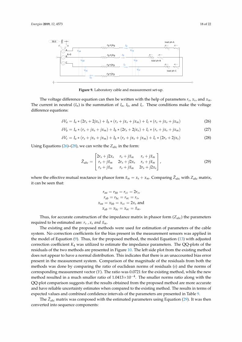
Figure 9 gives a basic overview of the laboratory cable and the measurement set-up. At the sourceend, there is a flexible and controllable voltage source and at the load end, there is a controllable loadbank. The load bank was controlled to vary the load over a period of time. To facilitate the estimationof mutual reactance, a voltage drop due to the mutual reactance is required. Unbalanced loading ofeach phase excites the voltage drops due to mutual reactances. Hence, the load of each phase was keptdifferent from each other. To model the laboratory cable, it was assumed that:

• Self-impedance of all the three phases and the return path (neutral) is the same;• Self-resistance of single core of the cable (all phases and neutral) : rs;• Self-reactance of single core of the cable (all phases and neutral) : xs;• Mutual reactance coupling between all the phases is the same: xm;• The mutual coupling effect of the neutral current on other phases is ignored.

Energies 2019, 12, 4573 18 of 22

++

+ +

+ +

A

B

C

Vf

R=0

50.0

Vsrc load ph-A

load ph-C

load ph-B

rs+jxs

rs+jxs

rs+jxs

rs+jxs

Vsa

Vsb

Vsc

Vra

Vrb

Vrc

In

Ia

Ib

Ic

Figure 9. Laboratory cable and measurement set-up.

The voltage difference equation can then be written with the help of parameters rs, xs, and xm.The current in neutral (In) is the summation of Ia, Ib, and Ic. These conditions make the voltagedifference equations:

δVa = Ia ∗ (2rs + 2jxs) + Ib ∗ (rs + jxs + jxm) + Ic ∗ (rs + jxs + jxm) (26)

δVb = Ia ∗ (rs + jxs + jxm) + Ib ∗ (2rs + 2jxs) + Ic ∗ (rs + jxs + jxm) (27)

δVc = Ia ∗ (rs + jxs + jxm) + Ib ∗ (rs + jxs + jxm) + Ic ∗ (2rs + 2jxs) (28)

Using Equations (26)–(28), we can write the Zabc in the form:

Zabc =

2rs + j2xs rs + jxm rs + jxm

rs + jxm 2rs + j2xs rs + jxm

rs + jxm rs + jxm 2rs + j2xs

, (29)

where the effective mutual reactance in phasor form xm = xs + xm. Comparing Zabc with Zabc matrix,it can be seen that:

raa = rbb = rcc = 2rs,rab = rbc = rac = rs,

xaa = xbb = xcc = 2xs andxab = xbc = xac = xm.

Thus, for accurate construction of the impedance matrix in phasor form (Zabc) the parametersrequired to be estimated are: rs , xs and xm.

The existing and the proposed methods were used for estimation of parameters of the cablesystem. No correction coefficients for the bias present in the measurement sensors was applied inthe model of Equation (9). Thus, for the proposed method, the model Equation (13) with adjustedcorrection coefficient K4 was utilized to estimate the impedance parameters. The QQ-plots of theresiduals of the two methods are presented in Figure 10. The left side plot from the existing methoddoes not appear to have a normal distribution. This indicates that there is an unaccounted bias errorpresent in the measurement system. Comparison of the magnitude of the residuals from both themethods was done by comparing the ratio of euclidean norms of residuals (s) and the norms ofcorresponding measurement vector (Y). The ratio was 0.0721 for the existing method, while the newmethod resulted in a much smaller ratio of 1.0413×10−4. The smaller norms ratio along with theQQ-plot comparison suggests that the results obtained from the proposed method are more accurateand have reliable uncertainty estimates when compared to the existing method. The results in terms ofexpected values and combined confidence intervals of the parameters are presented in Table 9.

The Zabc matrix was composed with the estimated parameters using Equation (29). It was thenconverted into sequence components:

Energies 2019, 12, 4573 19 of 22

Zabc =

0.190 + j0.0216 0.095 + j.0124 0.095 + j.01240.095 + j0.0124 0.190 + j.0216 0.095 + j.01240.095 + j0.0124 0.095 + j.0124 0.190 + j.0216

, Z012 =

0.380 + j0.0460.095 + j0.0090.095 + j0.009

.

The positive sequence resistance is quite close to the reference value measured by the DCmeasurement system. Further, the fact that the zero sequence impedance is about four times thepositive sequence impedance (especially for the resistance estimate) also suggests that the estimatesare supporting the considered cable model. For a 3-phase 4-wire system with neutral as a return path,it is known that:

(r + jx)0Seq = (r + jx)phase + 3 ∗ (r + jx)neutral (30)

and in this case, (r + jx)phase = (r + jx)neutral = (rs + jxs). This validates the condition stated inEquation (30).

This subsection demonstrated the application of the proposed method for cable parameterestimation for an LV cable in a laboratory. A comparison with the results from the existing methodwas done to show the superiority of the proposed method. The next section presents some generaldiscussion about the application of the proposed method in a real field.

-2 0 2

Standard Normal Quantiles

-0.2

-0.15

-0.1

-0.05

0

0.05

0.1

0.15

0.2

Qu

an

tile

s o

f In

pu

t S

am

ple

-4 -2 0 2 4

Standard Normal Quantiles

-0.1

-0.08

-0.06

-0.04

-0.02

0

0.02

0.04

0.06

0.08

Figure 10. Laboratory cable test: QQ-plot of the residuals for Equation (13) using the acquired data.Left plot: existing method, right plot: proposed method.

Table 9. Laboratory cable test: Expected parameters and corresponding CIs using both methods arepresented. The ratio of norm of residuals to the norm of expected parameter is also presented.

Method rs(Ω) CIrs (%) xs (Ω) CIxs (%) xm(Ω) CIxm (%) ||s||||Y||

Existing Method 0.0966 0.32 0.0117 6.60 0.0120 12.80 0.0721Proposed Method 0.0951 0.47 0.0108 3.55 0.0124 4.82 1.0413×10−4

6. Discussion

As no sensor comes without errors, it is important to estimate the performance of any applicationin their presence. The proposed method utilizes an overdetermined set of equations to estimate theparameters using OLS. The condition of the matrix H created using the available measurements couldalso play an important role in the quality of the results. The condition number κ for a full rank Hmatrix is a measure of uncertainty expected in the outcome of a mathematical operation on the matrixwhen its elements have errors. In short, it describes the sensitivity of the result obtained by an OLSestimator in the presence of the errors in the elements of the matrix H. A high condition numberimplies that the columns of the matrix H have a high correlation among them, making the matrixill-conditioned. It is shown in [13] that the expected variance of the parameters (θi) increases withincreasing the correlation between the columns hi of the matrix H. Hence, applications like 3-phaseparameter estimation which involve a high condition H matrix require high accuracy measurementset-ups. The columns of the matrix H are made up of the voltage and current measurements of

Energies 2019, 12, 4573 20 of 22

different phases. The independence of voltage and current signals in different phases would result inlower correlation between the columns of the H matrix. Hence, for the application of any OLS-basedmethod for cable parameter estimation in a 3-phase power system, apart from having high-qualitysensors, some degree of independence in the power-flows in the three phases is required. The effect ofcorrelation between power-flow in three phases on the accuracy of the proposed method is presentedin Table 10. Two different sets of power-flows on the cable were simulated. All the other characteristicslike measurement errors and data lengths were kept the same as in the previous simulation tests.

Table 10. Effect of conditioning of Matrix H.

rPF κH NB (%) NZ (%)

[0.9801 0.9799 0.9794] 7.94×103 0.402 1.769[0.9992 0.9996 0.9994] 2.54×103 0.403 18.495

In Table 10, rPF is the mutual correlation coefficients between power-flow in the three phases,κH is the condition number of the matrix H in corresponding power-flows, and NB and NZ are thenorms of the calculated percentage errors in the B and Z parameter vectors. It is observed that withless correlation in the power-flow in three phases, the proposed method performs better and givesmore accurate estimates. This realization could be used along with the idea presented in Section 4.2 toestimate the required accuracy of sensors for any application based on the prior knowledge about thecondition of the matrix H for a given system and for a desired level of accuracy.

Another important consideration while estimating the parameters for any general system isrealizing the underlying model of the system itself and designing the experiment for it. In the contextof the laboratory cable experiment, to estimate the mutual reactance component xm, it is importantto excite the mutual relationship between the current and the voltage signals. For this reason, thecurrents in three phases of the cable were kept different from each other by applying unbalanced loads.For balanced 3-phase conditions, the mutual components of the reactance might not be present, andusing the same cable system model could give wrong results. Hence, modeling the system correctly isequally important for accurate and reliable parameter estimates.

7. Conclusions

This paper presents a new method for estimating the resistance, reactance, and susceptance(R, X and B) parameters for a 3-phase cable system. The new method is developed to facilitateaccurate monitoring of cable temperature in real time to establish flexible loading levels of thecables [3]. The real-time cable temperature could be accurately estimated by tracking the real-timeresistance of the cable. Hence, to estimate the cable temperature accurately, it is imperative to gethigh-accuracy resistance estimates. In the field, the temperature and hence the resistance of thecables vary continuously depending on the conditions, such as current magnitude, ambient soiltemperature, and moisture content of the soil. There would be no correct reference to validate theestimated parameters, and thus, the calculation of the uncertainty of the resistance estimates is of equalimportance. Hence, uncertainties in the estimated parameters are calculated accurately and presentedas confidence intervals.

Using simulations and a laboratory test, it was shown that the regression model used in theproposed method can estimate these cable parameters with a better accuracy when compared tothe existing method. The OLS-based proposed estimation method is sensitive to the errors inthe measurement. The performance of the proposed method in the presence of random and biasmeasurement errors was investigated. To calculate the uncertainties of the estimates, new methodswere presented and compared. It was shown that the total uncertainty is made up of two parts,one due to the random errors in the measurement and the second due to a fixed bias caused eitherby inherent bias in the measurement sensors or caused by errors in the used system model. Theboundaries for deviations in the parameters were calculated when the measured signals had both

Energies 2019, 12, 4573 21 of 22

random and fixed errors. It was also shown that utilization of a correct model of both the cable systemand measurement chain is key to estimating the parameters more accurately and also estimatingcorrect uncertainties. In the end, results from a laboratory test to estimate the parameter of a cablesystem were presented. The results from the laboratory test also showed that the proposed methodwas able to achieve more accurate and precise estimates in the presence of both random and bias errorsin the sensors. The tests and the results showed that the proposed method is more suitable to estimateparameters of a 3-phase cable system in the field where the measurement equipment has unknownbias and random-error-related uncertainties.

Author Contributions: Conceptualization, R.S.S. and H.v.d.B.; Data curation, R.S.S. and S.B.; Investigation,R.S.S.; Methodology, R.S.S.; Project administration, V.C.; Supervision, S.C.; Writing—original draft, R.S.S.;Writing—review and editing, R.S.S., H.v.d.B., S.B., S.C., and V.C.

Funding: This work has received funding from the European Union’s Horizon 2020 research and innovationprogramme MEAN4SG under the Marie Skłodowska-Curie grant agreement 676042.

Conflicts of Interest: The authors declare no conflict of interest.The funders had no role in the design of the study;in the collection, analyses, or interpretation of data; in the writing of the manuscript, or in the decision to publishthe results.

References

1. Lee, J. Automatic Fault Location on Distribution Networks Using Synchronized Voltage Phasor MeasurementUnits. In Proceedings of the ASME 2014 Power Conference, Baltimore, MD, USA, 28–31 July 2014; pp. 1–5.

2. Sachdev, M.S.; Agarwal, R. A technique for estimating transmission line fault locations from digitalimpedance relay measurements. IEEE Trans. Power Deliv. 1988, 3, 121–129. [CrossRef]

3. Singh, R.S.; Cobben, S.; Gibescu, M.; van den Brom, H.; Colangelo, D.; Rietveld, G. Medium Voltage LineParameter Estimation Using Synchrophasor Data: A Step Towards Dynamic Line Rating. In Proceedingsof the 2018 IEEE Power Energy Society General Meeting (PESGM), Portland, OR, USA, 5–10 August 2018;pp. 1–5. [CrossRef]

4. Shi, D.; Tylavsky, D.J.; Logic, N.; Koellner, K.M. Identification of short transmission-line parameters fromsynchrophasor measurements. In Proceedings of the IEEE 2008 40th North American Power Symposium,Calgary, AB, Canada, 28–30 September 2008; pp. 1–8. [CrossRef]

5. Shi, D.; Tylavsky, D.J.; Koellner, K.M.; Logic, N.; Wheeler, D.E. Transmission line parameter identificationusing PMU measurements. Eur. Trans. Electr. Power 2011, 21, 1574–1588. [CrossRef]

6. Ritzmann, D.; Wright, P.S.; Holderbaum, W.; Potter, B. A Method for Accurate Transmission Line ImpedanceParameter Estimation. IEEE Trans. Instrum. Meas. 2016, 65, 2204–2213. [CrossRef]

7. Ritzmann, D.; Rens, J.; Wright, P.S.; Holderbaum, W.; Potter, B. A novel approach to noninvasivemeasurement of overhead line impedance parameters. IEEE Trans. Instrum. Meas. 2017, 66, 1155–1163.[CrossRef]

8. Milojevic, V.; Calija, S.; Rietveld, G.; Acanski, M.V.; Colangelo, D. Utilization of PMU Measurements forThree-Phase Line Parameter Estimation in Power Systems. IEEE Trans. Instrum. Meas. 2018, 67, 2453–2462.[CrossRef]

9. Menditto, A.; Patriarca, M.; Magnusson, B. Understanding the meaning of accuracy, trueness and precision.Accredit. Qual. Assur. 2007, 12, 45–47. [CrossRef]

10. JCGM 100:2008, Evaluation of Measurement Data—Guide to the Expression of Uncertainty in Measurement; JointCommittee for Guides in Metrology: Sèvres, France, 2008.

11. JCGM 102:2011, Evaluation of Measurement Data—Supplement 2 to the "Guide to the Expression of Uncertainty inMeasurement; Joint Committee for Guides in Metrology: Sèvres, France, 2011.

12. Khandeparkar, K.V.; Soman, S.A.; Gajjar, G. Detection and Correction of Systematic Errors in InstrumentTransformers Along With Line Parameter Estimation Using PMU Data. IEEE Trans. Power Syst. 2017,32, 3089–3098. [CrossRef]

13. Greene, W.H. Econometric Analysis, 5th ed.; Pearson Education: London, UK, 2003.14. Golub, G.H.; Van Loan, C.F. Matrix Computations, 3rd ed.; The Johns Hopkins University Press: Baltimore,

MD, USA, 1996.

Energies 2019, 12, 4573 22 of 22

15. Higham, N. Accuracy and Stability of Numerical Algorithms, 2nd ed.; Society for Industrial and AppliedMathematics: Philadelphia, PA, USA, 2002. [CrossRef]

16. Olive, D.J. Linear Regression; Springer International Publishing: Cham, Switzerland, 2017; p. 254. [CrossRef]17. Arbiter Systems, Inc. Model 1133a Power Sentinel Power Quality Revenue Standard Operation Manual; Arbiter

Systems, Inc.: Paso Robles, CA, USA.

c© 2019 by the authors. Licensee MDPI, Basel, Switzerland. This article is an open accessarticle distributed under the terms and conditions of the Creative Commons Attribution(CC BY) license (http://creativecommons.org/licenses/by/4.0/).