Estimation of Life Tables in the Latin American Data Base (LAMBdA): Adjustments for Relative Completeness and Age Misreporting Alberto Palloni * Guido Pinto † HiramBeltr´an-S´ anchez ‡ October 27, 2016 1 Background The methodologies described in this paper belong to a small subset of a broader set of methods developed to produce adjusted estimates of adult mortality for countries in the Latin American and Caribbean (LAC) region covering 150-160 years, from 1850 to 2010. This period encompasses approximately the end of colonial rule, the aftermath of wars of independence from Spanish and Portuguese domination, the establishment of nation states, integration into a world system and the world economy, and all developments that unfolded following World War II. 1 In this paper we focus only on adjustments of life tables for the post-1950 period. To do so we avail ourselves of mortality data consisting of yearly deaths by age and gender and population censuses. Because methods to adjust for completeness of death registration are well-known we focus on the description of relatively new methods to adjust for adult age misreporting. We then combine these two methods in an evaluation study designed to identify an optimal strategy to construct adjusted life tables for adult ages. The paper is in six sections. In the first section we briefly define problems caused by defective vital statistics and census enumerations. In the second section we propose a model to represent the nature of adult age misreporting and in the third section we describe a methodology to detect and adjust for adult age misreporting. The fourth section describes an evaluation study designed to assess the performance of techniques to correct mortality indicators for both errors of coverage and age reporting. The fifth section discusses results from the evaluation study. The last section summarizes results and argues that adjustment of imperfect mortality data is subject to uncertainty and that treatment of the adjusted data is best carried out with models that account for uncertainty. 2 Errors affecting measures of adult mortality The post-1950 mortality data in LAC is limited by defective coverage and adult age misreporting. By and large, observed death counts are a variable fraction of the ‘true’ number of deaths that take * Center for Demography and Health of Aging, Center for Demography and Ecology, University of Wisconsin- Madison. Email: [email protected]. † Center for Demography and Health of Aging, Center for Demography and Ecology, University of Wisconsin- Madison. ‡ Department of Community Health Sciences & California Center for Population Research, Fielding School of Public Health, UCLA. Email: [email protected]. 1 We define as “adult” the population aged 5 and older and as “children” those younger than age 5. 1
Transcript
Estimation of Life Tables in the Latin American Data
Base (LAMBdA): Adjustments for Relative
Completeness and Age Misreporting
Alberto Palloni∗ Guido Pinto† Hiram Beltran-Sanchez‡
October 27, 2016
1 Background
The methodologies described in this paper belong to a small subset of a broader set of methodsdeveloped to produce adjusted estimates of adult mortality for countries in the Latin Americanand Caribbean (LAC) region covering 150-160 years, from 1850 to 2010. This period encompassesapproximately the end of colonial rule, the aftermath of wars of independence from Spanish andPortuguese domination, the establishment of nation states, integration into a world system andthe world economy, and all developments that unfolded following World War II.1 In this paper wefocus only on adjustments of life tables for the post-1950 period. To do so we avail ourselves ofmortality data consisting of yearly deaths by age and gender and population censuses. Becausemethods to adjust for completeness of death registration are well-known we focus on the descriptionof relatively new methods to adjust for adult age misreporting. We then combine these two methodsin an evaluation study designed to identify an optimal strategy to construct adjusted life tables foradult ages.
The paper is in six sections. In the first section we briefly define problems caused by defectivevital statistics and census enumerations. In the second section we propose a model to representthe nature of adult age misreporting and in the third section we describe a methodology to detectand adjust for adult age misreporting. The fourth section describes an evaluation study designedto assess the performance of techniques to correct mortality indicators for both errors of coverageand age reporting. The fifth section discusses results from the evaluation study. The last sectionsummarizes results and argues that adjustment of imperfect mortality data is subject to uncertaintyand that treatment of the adjusted data is best carried out with models that account for uncertainty.
2 Errors affecting measures of adult mortality
The post-1950 mortality data in LAC is limited by defective coverage and adult age misreporting.By and large, observed death counts are a variable fraction of the ‘true’ number of deaths that take
∗Center for Demography and Health of Aging, Center for Demography and Ecology, University of Wisconsin-Madison. Email: [email protected].†Center for Demography and Health of Aging, Center for Demography and Ecology, University of Wisconsin-
Madison.‡Department of Community Health Sciences & California Center for Population Research, Fielding School of
Public Health, UCLA. Email: [email protected] define as “adult” the population aged 5 and older and as “children” those younger than age 5.
place at a particular time as they exclude events that, for a number of reasons, are never recorded.Since population censuses too are normally affected by coverage problems, mortality rates computedwith the raw data may contain smaller net errors that would be expected otherwise. In general,however, the observed mortality rates underestimate mortality levels, particularly at very youngand old ages. We use the term relative completeness when we speak of ratios of observed to truemortality rates.
Table 1 displays estimates of relative completeness of adult (over 5 years of age) and, forcomparison, those corresponding to infant (age 0) and early child (ages 1-4) death registration ina sample of LAC countries over two different periods of time. The figures in this table confirmthat the quality of the information is poorer at very young ages and that, although there is a clearuniversal trend toward improvement, an important fraction of countries still show signs of deficientregistration even quite recently.
Imperfect relative completeness of death registration is not the only problem affecting estimatesof mortality. An important domain of errors involves age misreporting and the most insidiousmanifestation is systematic over (under) reporting. Vital and census statistics in LAC countriesare, almost without exception, affected by age overstatement, particularly at ages over 40 or 45(see below). When the (true) age distribution of a population is roughly exponential in nature —asit always is in stable and quasi stable populations—systematic age overstatement of populationsinduces downward biases in mortality rates at older ages. These biases are not offset when there isan equal propensity to overstate ages at death. The reason these two type of errors do not canceleach other out is that while both adult mortality rates and adult population age distributions areroughly exponential, one slopes upwards (mortality rates) whereas the other slopes downwards(population). Matters are made worse when, as is almost always the case, the rate of decrease ofpopulation with age (natural rate of increase in a stable population) is several times lower thanthe rate of increase of adult mortality rates (rate of senescence in Gompertz mortality regimes).The consequence is that unless the propensity to overestimate ages at death is much higher thanthe propensity to overestimate ages of population, observed mortality rates will contain downwardbiases. If left uncorrected, the resulting life tables will offer a misleading portrayal of the curvatureof mortality at older ages, suggesting the existence of slower rates of senescence or heavy influenceof selection due to changing frailty composition. As the quality of vital registration and censusenumeration improves, the magnitude of these biases tends to decrease and the entire history ofobserved life tables will erroneously suggest trends in old age patterns of mortality and even relativeacceleration of the rates of mortality decline at older ages.
Unlike problems created by age heaping, distortions caused by systematic age misstatementcannot be repaired by restoring the original age distribution standard using computations thatrely on safe assumptions. Systematic age misstatement is altogether different since it is harder todiagnose and, as we show below, its treatment requires additional knowledge of two functions: (a)the conditional (on age and gender) propensity of individuals to exaggerate (decrease) the true ageand (b) the conditional (on age and gender) distribution of the difference between the correct anddeclared age. To solve the problem we propose generalizations of an existing procedure to identifythe presence of age misstatement, formulate a new method to estimate functions describing (a) and(b) from observables, and define an algorithm that adjusts observed adult mortality rates for bothfaulty coverage and systematic age misreporting.
Table 2 displays estimated biases in mortality rates at ages over 45 in a sample of country-yearsused in our analysis and the corresponding errors in life expectancy at age 60.
The problems generated by defective completeness of death registration as well as alternative
2
Table 1: Relative completeness of deaths registration in the LAC countries: 1920-2010.
CountryPeriod 1900-1949 Period 1950+
Mid-Year Age 0 Age 1-4 Age 5+ Mid-Year Age 5+
Argentina 1914 0.968 0.865 0.939 1953 0.9742005 0.995
adjustments procedure to deal with it are well-known. Much less is known about the nature andimpact of age misreporting. In the section below we propose a methodology to identify the presenceof these errors and to correct them.
3 Systematic age misreporting
3.1 Setup
We begin with a few basic definitions. Let θox be the average conditional probability that individualsaged x overstate their age in a census and θux the conditional probability of understating their age.Then (1 − θox − θux) is the probability of an accurate age statement. Individuals who over(under)state their age do so by choosing, not always randomly, the age declared and observed in the census.This age could be n > 0 years removed from the true age. As we show below, it suffices to let nrange between 1 and 10+ since the frequencies for values of 10 years and above are exceedinglysmall, e.g. individuals rarely over(understate) their age by more that ten digits. Let ρox(n) bethe average conditional probability that individuals aged x who overstate ages will do so by nyears with an analogous definition for the probabilities for age understatement, ρux(n) and with∑
n ρux(n) =
∑n ρ
ox(n) = 1. To compute the observed number at age y, Poy, we consider the true
number at that age P Ty , and apply the conditional probabilities defined above:
P oy = P Ty (1− θox − θux) +
j=10∑j=1
P Ty−jρoy−j(j)θ
oy−j +
j=10∑j=1
P Ty+jρuy+j(j)θ
uy+j . (3.1)
This expression can be generalized for all ages between 0 and 100 in compact matrix notation:
Πo = ΘΠT (3.2)
where Πo is the (101x1) observed population vector, ΠT is the (101x1) true population vector andΘ is a 101x101 square matrix of “transition” probabilities, e.g. the probabilities of migration into orout of single year age-groups. In particular, the diagonal of Θ contains the probabilities of correctlydeclaring ages, (1−θox−θux), and entries in the off-diagonal row k for columns k−1, k−2, . . . , k−10are the values ρoy−1(j)θ
oy−1, . . . , ρ
oy−10(j)θ
oy−10 whereas those in columns k+1, k+2, . . . , k+10 are the
values ρuy+1(j)θuy+1, . . . , ρ
uy+10(j)θ
uy+10. One can retrieve the matrix with the true age distribution
of the population after pre-multiplying the previous expression by the inverse of Θ−1, that is
Θ−1Πo = ΠT , (3.3)
an operation that requires full knowledge of the matrix Θ. As we show below, demographers haveonly superficial information about the nature of this matrix in LAC countries or anywhere elsefor that matter (but see Bhat (1990)). In the absence of precise knowledge of the probabilitiescontained in the matrix one could adopt shortcuts, simplifications that circumvent knowledge gapsbut that, as shown below, lead to identification problems, most of which translate into inability tospecify an invertible matrix of transition probabilities.
5
3.2 Observed patterns of age misreporting
What do we know about age misreporting in population and death counts in LAC and in othercountries? There is an extensive literature on general errors in age reporting (Ewbank, 1981;Chidambaram and Sathar, 1984; Kamps E., 1976; Nunez, 1984) as well as on systematic age mis-statement, mostly adult age overstatement, in population counts. And while a fair number of thesestudies uncover evidence of overstatement in low income countries (Mazess and Forman, 1979;Grushka, 1996; Bhat, 1987, 1990; Del Popolo, 2000; Dechter and Preston, 1991) or in US migrant(Hispanic or Hispanic origins) groups (Rosenwaike and Preston, 1984; Spencer, 1984), there is abody of literature that identifies patterns of age overstatemet in high income countries as well (Ho-riuchi and Coale, 1985; Coale and Kisker, 1986; Condran et al., 1991; Preston et al., 2003; Elo andPreston, 1994). In the US, for example, age overstatement is one of the factors that could explainthe so called Black-White mortality crossover, whereby African American mortality rates dip belowthose of their White counterparts at very old ages (over 70). And while the recurrent idea of heavyselection due to frailty has not been completely discarded, the most recent investigations suggestthat overstatement of ages in the population (and also deaths) among African American more sothan among Whites accounts for a substantial part of the mortality crossover (Elo and Preston,1994). The Black-White mortality crossover is just an extreme example of the damage that agemisreporting can inflict on estimates of adult mortality. As others before us have done (Dechterand Preston, 1991; Grushka, 1996; Bhat, 1987, 1990), we will show that age overstatement is alsoan important source of error in LAC countries.
Partial information on the matrix Θ has been obtained mostly from studies involving recordlinkages (Elo and Preston, 1994; Preston et al., 1996; Rosenwaike and Preston, 1984; Rosenwaike,1987), post enumeration surveys (Ortega and Garcia, 1985) and comparisons of two independentlygathered data sources that should produce the same outcomes (Bhat, 1990). In all these studies,however, the information is either aggregated in five-year age groups or applies to populations withlevels of education that are much higher than those in LAC countries. Lack of age detail is prob-lematic since computation of conditional probabilities in coarse age groups rests on approximationsthat, if violated, are generally harmful to the accuracy of estimates. Using a transition matrixappropriate for a population with higher or lower levels of education or literacy than the target onemay lead to distortions since age misstatement is strongly associated with levels of education.
3.3 Misreporting of ages of population
To circumvent the foregoing problems we take advantage of a 2002 evaluation study launched bythe Central American Center for Population at the University of Costa Rica. The program wasdesigned to assess the quality of information of death registration and the accuracy of the 2000census counts2. One of the components of this study was a linkage of an age stratified sampleof 9,113 individual census records with the national voter registers, a database that contains ageinformation from birth certificates. A total of 7426 records were matched corresponding to 81.5%of the original sample and 86.6 % of the non foreign born part of the sample. The final data setcontains individuals classified by gender, education and other traits, and by ‘true’ and declaredage. To estimate the entries of matrix Θ we proceeded in two steps:
i Estimation of probabilities of age over and understatement, θox(V ) and θux(V ) where V is avector of individual characteristics, including age: We first estimate a logistic model for a
2We are grateful to Drs. Gilbert Brenes and Luis Rosero Bixby from the Central American Population Center atthe University of Costa Rica for having provided tabulations we used in this study.
6
binary variable set to 1 when there is over (under) statement and zero otherwise. Initiallythe model specifies a vector of covariates including age, age squared, urban/rural residence,gender, and education. The sample includes individuals aged 50 and over since at youngerages there are only traces of systematic age misstatement (mostly in the form of heaping).Because gender and age are the only covariates that can be used at a national level, wesimplify the model to include only these two traits as predictors. Finally, after verifying thatthe effects of age squared and gender were statistically insignificant, the final model conditionsonly on ‘true’ age of individuals. Table 3 displays estimated parameters for over and understating ages using the weighted sample.
ii Estimation of conditional probabilities of over(under) stating ages by 1 < n ≤ 10 years, ρox(j)and ρux(j): We estimate a multinomial model with 9 categories that includes gender and(true) continuous age as independent variable. The resulting estimates reveal that the effectsof gender are always statistically insignificant, that those of age show no clear pattern and, inaddition, that their magnitude is quite small in 6 out of 8 cases for overstatement models andin 5 out of 8 contrasts for age understatement. To simplify we estimate a null model predictingthe average conditional probabilities of exaggerating (or diminishing) by n years applicableto all ages older than 50 and both genders. The values of the predicted probabilities of overand understating the true age are in Table 4.
Although it is now possible to compute an estimator of the target mobility matrix, Θ, thereremains a knotty problem of identification that cannot be resolved without additional simplifica-tions. Suppose, for example, we seek to estimate mortality trends in a country with much lowerlevels of education than in Costa Rica. Replacing Θ for the true matrix in (3.3), we will obtain atrue distribution of ages but only under the very strong assumption that age misstatement is iden-tical across countries. This contradicts accumulated knowledge showing that the severity of agemisstatement increases as levels of education drop. A less constraining assumption is to argue thatwhile the age pattern of misstatement is identical across countries, the levels could be different. Toexpress this one could think of multiplying the conditional probabilities of over and under statingages (or a monotonic transform of it) by some constant, say φo and φu for over and understatementrespectively. While this is a reasonable strategy it generates an additional problem, namely, that aunique solution for equation (3.2) may no longer be possible since different combinations of φo andφu embedded in the transition matrix could plausibly yield identical results. To circumvent this newdifficulty we propose a standard pattern of probabilities of net age overstatement as ϕSx = θox − θuxand then apply to it the conditional probabilities of overstating one’s age by n years (the ρox(j)values defined before). Under these conditions the off-diagonal cells of the matrix defined by ϕSx ,ΘS , simplify as all entries involving age understatement become zeros. This makes identificationmore likely and the search for a unique solution of φno, a parameter measuring the magnitude ofthe net overstatement (no) relative to the standard pattern, a more feasible enterprise.
There are two conditions required for this standard pattern to play a helpful role. The firstis that the probabilities of age overstatement always be larger than the probabilities of age under-statement. The second is that the conditional distribution of n, the integer number of years bywhich individuals exaggerate (diminish) their true age, be approximately the same among thosewho over and understate ages. Figure 1 displays predicted probabilities of over and understatingages by age, θox − θux , Figure 2 displays the differences ϕSx = θox − θux , and Figure 3 shows predictedconditional probabilities of over stating ages by n years with 0 < n ≤ 10 or ρox(j). These figuresshow that the first condition is always satisfied whereas the second is only approximately met in
7
Table 3: Estimated parameters of best logistic models for age misreporting.
1 Regressions estimated using sampling weights. Sample includes population with true age 60 andolder and excludes ambiguous cases and foreign citizens.
Table 4: Average (conditional) probabilities of overreporting ages.
1Predicted values computed from a null multinomial logistic model with 10 categories, n=1786(males and females). Estimation using sampling weights. Figures may not add up to 1 due to
rounding errors.
these data. However, differences are minor and are found mostly at higher values of n, where theprobabilities of over(under) stating are small. We define these two items, the pair of age-specificdifferences between predicted probabilities of over and under statement (Table 3) and the associ-ated conditional probabilities of overstating by n years (Table 4), to be the standard pattern of agenet overstatement3.
3.4 Misreporting of ages at deaths
The developments above only refer to age misreporting in population counts. However, it is knownthat mortality rates are also influenced by age misreporting of ages at death (Rosenwaike, 1987).The nature of the problem in this case is somewhat different since it is not the decedent thatdeclares the age at death but a kin or someone else unrelated to the decedent. A handful of studies
3The representation we used throughout suggests that patterns of age misreporting in any country is a multipleof the standard pattern. Although this helps the algebra and statement of proofs, we cheat in our computationsand follow a roundabout algorithm. In fact, we generate new patterns of values from the standard by defining thefunction logit(ϕix) = α+ βlogit(ϕSx ), set the value of β equal to 1, and then identify the level of age overstatementin a population i by fixing α so that ϕix ∼ φoϕSx and φo is the desired level of age over reporting.
8
Figure 1: Predicted probabilities of over(under) stating ages.
Probability of overstatingProbability of understating
●
●
Source: Costa Rica Special study of 2000 population census.
Figure 2: Predicted probabilities of net overstating ages.
Age
Net
pro
babi
lity
of o
vers
tatin
g
0.05
0.10
0.15
45 50 55 60 65 70 75 80 85 90 95 100
0.05
0.10
0.15
●●
●●
●●
●●
●●
●●
●●
●●
●●
●●
●●
●●
●●
●●
●●
●●
●●
●●
●●
●●
●●
●●
●●
●●
●●
●●
●●
●●
Source: Costa Rica Special study of 2000 population census.
9
Figure 3: Conditional probabilities of overstating age by n years.
Number of years over(under)statement
Pro
babi
lity
of o
vers
tatin
g n
year
s
0.00
0.20
0.40
0.60
1 2 3 4 5 6 7 8 9 10
0.00
0.20
0.40
0.60●
●
●
●●
● ● ● ● ●
Source: Costa Rica Special study of 2000 population census.
based on record linkages show that there is age misreporting of ages at death as well, albeit of lowermagnitude than that found in population counts, and that it also tends to be in the direction ofoverstatement (Rosenwaike and Preston, 1984). This is confirmed by the application of indirecttechniques designed to detect age at death overstatement in a number of low and high incomecountries (see below). It follows that expressions analogous to (3.1) and (3.2) must be applicablefor death counts as well. To make the problem tractable one needs an empirical approximation toa matrix analogous to Θ but now specialized to ages at death. To our knowledge no such matrixhas ever been estimated in LAC or anywhere else and we are unaware of any national data thatcould be used for such purpose. In what follows we assume that the standard age pattern of agemisstatement of death counts is identical to that of age misstatement of population counts, althoughits level may be different. This assumption enables us to define the final model of age misreportingas a set of two equations with two unknown parameters:
Πo = φnoΘSΠT (3.4)
∆o = λnoΘS∆T (3.5)
where ∆T and ∆O are the true and observed distributions of death counts and λno is the magnitudeof net overstatement of ages at death relative to the standard pattern. In closed populationsequations (3.4) and (3.5) are naturally (see below) related and it is unlikely that there is alwaysa unique solutions for φno and λno unless we either fix the value of one of them or, alternatively,retrieve solely their ratio. A brief proof of lack of identification is in Appendix B and solutions forempirical estimation are in section 4.2.
10
4 Identification and correction of errors due to systematic agemisreporting
In this section we propose a methodology to identify and then adjust mortality statistics for agemisreporting. The methodology is only applicable when age misreporting is produced following themodel outlined in the previous section.
4.1 Identification of systematic age misreporting
A key component of our analysis is the detection and identification of patterns of age misstatementin the population and death counts. As shown in a previous section, the distortions associated withage misreporting in population and death counts is more complex than those involving only faultycompleteness. Detection of the problem is difficult since its manifestations are quite subtle and,in the absence of overt and striking phenomena such as the US Black-White cross over, is likelyto remain concealed and undetected. There are two well-tested methods to identify the existenceof age over(under) statement in either population or death counts. The first method requires anexternal data source with correct dates of birth or ages in a population at a particular time thatcan be compared to age-specific census counts at approximately the same time. An example ofthis is the utilization of Medicare data in the US, a source of information that, as a rule, containsboth population exposed and mortality data. Because Medicare data are linked to Social Securityrecords and these are known to register age with high precision, mortality rates computed fromMedicare data are a gold standard against which conventional mortality rates could be contrastedand their quality evaluated (Elo et al, 2004). If one ignores the existence of a population notcovered by Medicare records, it is also feasible to link individual census records to Medicare recordsand investigate more precisely the nature of patterns of age misreporting in census counts. If, inaddition, Medicare records are linked to the US National Death Index (NDI) it is then possibleto repeat the same operations and assess the quality of reporting of age at deaths. In all casesone must assume that the coverage of population in both sources is complete or, if incomplete,identical4. Record linkage from multiple sources such as those illustrated above has rarely beenused as it is expensive and involves resolution of complicated confidentiality issues.
A second method is less data demanding, considerably less expensive and is simple to applybut can only reveal the existence of age misreporting in one of the two sources and provides fewclues about its nature. The procedure was proposed by Preston and colleagues (Rosenwaike andPreston, 1984; Elo and Preston, 1994; Bhat, 1990; Grushka, 1996) and has been applied in countriesof North America, Western Europe and in Latin America (Condran et al., 1991; Grushka, 1996;Dechter and Preston, 1991; Palloni and Pinto, 2004; Del Popolo, 2000). In a nutshell the methodconsists of comparing cumulative population counts in a census in year t1 to the expected cumulativepopulation counts in a second population census in year t2. The computation of expected quantitiesrequires both an initial census opening the intercensal interval, a second census counts at time t2closing the intercensal interval, and age specific deaths counts in the intercensal period spanningan interval of k = (t2 − t1 + 1) years. The ratio of observed to expected population is an indicatorof age misstatement:
cmRox,[t1,t2] =cmP ox+k,t2/cmP
ox,t1
1− (cmDox,[t1,t2]
/cmP ox,t1)(4.1)
4The assumption is more restrictive than we made it sound: if population coverage is not complete in either source,then the subpopulations missed in each census must be random relative to their true and reported age.
11
where cmP ox,t1 and cmP ox,t2 are cumulative populations over ages x and x+k in the first and secondcensus, respectively, and cmDo
x,[t1,t2]is the cumulative deaths after age x during the intercensal
period. This expression is a simple contrast between two different estimates of the same underlyingquantity (population parameter), namely, the cumulative survival ratio: the denominator uses thecomplement of the observed ratio of (cumulative) intercensal deaths to (cumulative) populationin the first census, whereas the numerator expresses it as the survival ratio computed from thecumulative counts in two successive population censuses. It is useful to express (4.1) in a logarithmicform, namely,
ln(cmRx,[t1,t2]) = ln(SNox,x+k)− ln(SDo
x,x+k) (4.2)
where SNox,x+k is the ‘survival ratio’ computed from two censuses and SDo
x,x+k is the survival ratio
computed from intercensal deaths5. In the absence of migration, age misstatement and imperfectcompleteness of census and death counts, both estimators should yield the same number, the ratioin (4.1) should be 1, and the log expression in (4.2) should be 0 for all adult ages.
To shed light on the meaning of expressions (4.1) or (4.2) and to simplify notation and termi-nology we will speak of net age misreporting to refer to the net result of both age over and understatement. Furthermore, because we, as well as past research, uncover systematic net age overstate-ment of adult ages in LAC countries, we will speak of ‘age overstatement’ or ‘age overreporting’even though we refer to the net result of age under and over reporting. In Appendix C we showthat when the assumption of absence of age misreporting is violated, we can approximate (4.2) as
ln(cmRx,[t1,t2]) ∼ ln
(h(x+ k)
h(x)
)−(g(x)
h(x)− 1
)(1 + ITx,x+k
)(4.3)
where ITx,x+k is a true integrated hazard analogue between ages x and x + k (and hence strictlypositive), h(x) is an increasing function of age that depends on age overstatement of populationsand g(x) is an increasing function of age that depends only on overstatement of ages at death. Bothh(x) and g(x) are functions of the propensity to overstate and the underlying population and deathsage distribution. Assume now that the propensity to overstate ages (of populations or deaths) isage invariant or increases with age and that the following three conditions hold: (a) the (true) agedistribution slopes sharply downward, (b) the age distribution of deaths increases with age, and(c) the rate of decrease of population with age is smaller that the rate of increase of deaths withage. Under these three conditions, almost universally verified in all human populations, the ratioh(x + k)/h(x) will always be larger than 1 and will increase with age, g(x) will always be largerthan 1 and increase with age, and the rate of increase in g(x) will exceed the rate of increase inh(x) so that g(x) > h(x) almost everywhere in the age span. The following are possible scenarios6:
1. When there is systematic age overstatement of population counts ONLY, h(x) > 1 andg(x) = 1, then expression (4.3) reduces to
ln(cmRx,[t1,t2]) = ln
(h(x+ k)
h(x)
)+ (h−1(x)− 1)(1 + ITx,x+k) < 0
5In Appendix C we provide terminology and a full justification for the use of this index.6The impact of age misreporting predicted analytically in these scenarios has been confirmed by simulation studies
(Condran et al., 1991; Palloni and Pinto, 2004; Grushka, 1996). In section 6 we show that our simulations also accordwith analytic predictions.
12
The inequality results because the positive term in the expression, that is, the distortion of thesurvival ratio based on population counts, will be smaller than the negative term influencedby the distortion in the second estimator based on intercensal death rates.
2. When there is systematic age overstatement of death counts ONLY, h(x) = 1 and g(x) > 1,the expression becomes
ln(cmRx,[t1,t2]) = ln
(h(x+ k)
h(x)
)+ (g(x)− 1)(1 + ITx,x+k) > 0
and the positive sign results from the fact that all terms in the expression are positive.
3. When there is systematic overstatement of BOTH population and death counts, g(x) >h(x) > 1, then
ln(cmRx,[t1,t2]) = ln
(h(x+ k)
h(x)
)+
(g(x)
h(x)− 1
)(1 + ITx,x+k) > 0
because, by assumption, all terms are positive.
Before we can use the above to diagnose conditions in an empirical case, two issues must beresolved. First, it is possible that there are empirical patterns of age overstatement of deaths andpopulations that offset each other and produce ratios close to 1 even though the underlying dataare incorrect. That is, scenario (3) is such that the log of the ratio is 0 at all ages even when thereis net age overstatement. Because of this possibility, a diagnostic of observed conditions based onthe index (or the log of the index) can only detect consistency (including error consistency) of agedeclaration in population and death counts, rather than suggest accuracy (Dechter and Preston,1991). Second, throughout we assumed that both census and death counts had perfect coverage.When one allows for defective census coverage, an identification problem is created since now wewill have
ln(cmRx,[t1,t2]) ∼ ln
(C2
C1
)+ ln
(f(x+ k)
f(x)
)−(C3 · g(x)
C1 · h(x)− 1
)(1 + ITx,x+k) (4.4)
and it is clear that we can no longer separate the role of age overstatement and completeness. Inparticular, even if there is no age misreporting, expression (4.4) can yield non-zero values and mimicincreasing or decreasing patterns with age that result naturally from age overstatement alone. Tounderstand better the combined influence of defective coverage and age misreporting on observedmortality rates we need to define more precisely the nature of the functions h(x) and g(x), thenature of their dependence on patterns of age misreporting and how they interact with defectivecoverage. We investigate this issue in the section below.
4.2 Correction of errors due to age misreporting
As indicated before, the main tool to detect adult age misreporting is highly sensitive to relativecompleteness of census counts. Figure 4 displays the value of cmRx that one obtains when thereis no age misreporting at all but there is differential completeness in census counts. Thus, onecannot learn much about patterns of age misreporting unless population census counts are firstadjusted. This requires to identify methods that provide robust estimates of completeness of onecensus relative to the other. As we show below, the evaluation study confirms a result first noted
13
Figure 4: Behavior of index of age misstatement with differential censuses.
Age
Cum
ulat
ive
surv
ival
rat
io
0.0
0.2
0.4
0.6
0.8
1.0
45 50 55 60 65 70 75 80 85 90 95 100
Observed
0.9999990
0.9999995
1.0000000
1.0000005
1.0000010
45 50 55 60 65 70 75 80 85 90 95 100
Adjusted
by Ken Hill (Hill et al., 2009) and shows that the modified Brass technique (Brass-Hill) producesa robust estimate of C1/C2. The ratio of completeness factor is sufficient to correct the observedvalues of cmRx.
Once the ratios are adjusted there remains the task of retrieving estimates of the magnitudeof net adult age net overstatement. The model developed before based on a known standard of agenet overreporting includes two parameters, λno and φno for the magnitude of population age overand understatement, respectively. There are three different methods to estimate these parameters.
i A brute force method : it is possible, but not advisable or even necessary (see (ii) below), touse the cumbersome but exact procedure that consists of computing the values for the vector[cmRx=45,100] that can be generated by combinations of the known vectors [α1x=45,100] and[α2x=45,100] and multiple pairs (λno, φno) and then choose the (unique) pair of values that bestreproduces the observed vector [cmRx=45,100]
ii Parametric method I : this method is a short cut for Method I. We used simulated data toestimate the following relation
(cmRx)−1 = α0x + α1xλno + α3xφ
no (4.5)
for all values of x ≥ 45. The parameters of this relation, α0, α1 and α3, characterize thespace of solutions for the triplet (cmRx, λ
no, φno) embedded in the simulated data. As shownbelow in Table 5 the fit of the model is very good and the estimated values of the constantis always close to 1, as it should be. If the observed data is an element of the space ofsolutions, that is, if the observed data is generated by one of the combinations of parametersthat spawns the simulation, it might be possible to invert the procedure in (4.5), use the
14
coefficients estimated from (4.5) and compute the pair of values (λno, φno) that reproducesthe observed value cmRx − 1 for all x7. We show in Table 6 that given an observed vector ofvalues {cmRx=45,100} and the vectors of parameters {α1x=45,100} and {α3x=45,100} there is aunique and best (in mean squared error sense) solution for the unknown parameters of model(4.5) 8.
iii Parametric method II : the third method seeks to reproduce the shape of the function [cmRx=45,100]as a function of age and then map parameters of the function onto the pairs (λno, φno) thatgenerated the data. It consists of fitting a hyperbola to a range of values of cmRx
cmRx = β1/(ς − age)β2 (4.6)
where ς is set equal to 769. We then use the estimated parameters of function (4.6) to predictthe pair of values (λno, φno). As we show in Table 7 the fit of the hyperbolic function tothe distorted data is very tight but the retrieval of the hidden parameters governing net ageoverstatement is generally poor. This is due to under-identification: if one uses the entirerange of values attainable by λno and φno, the function cmRx=45,100 can be mapped ontomultiple pairs (λno, φno). The procedure works best when the pair of values (λno, φno) iswithin a limited range (approximately [0.10-1.5]). Because of this regularity one can usemethod (ii) and (iii) jointly to seek consistency: if the observed values of the parametersλno and φno are within the identification range, then both methods should produce the sameresults.
5 Evaluation study
The nature of problems generated by faulty national vital statistics and censuses is highly het-erogeneous and vary by country, time period, age groups, gender and surely by regions. This iscomplicated by the fact that there are multiple techniques or procedures, each relying on specializedassumptions, to adjust for errors that exist in the data. Over the last two to three decades, butmostly in the late seventies and eighties, demographers developed a large number of techniques toadjust faulty data from censuses, vital statistics and population surveys to estimate both fertilityand mortality. There are nearly 15 different, albeit not completely independent methods, to correctfor completeness errors (but not age misreporting) of adult mortality statistics, each with its ownpeculiar advantages and shortcomings, and each depending on sets of different but overlappingassumptions.
Optimal adjustments for faulty coverage and age misreporting are unfeasible in the absenceof well-established criteria to decide which candidate techniques performs optimally and underwhich conditions they do or do not do so. To assess the performance of alternative procedures and
7The constrain imposed, namely, that the observed data must be in the space of populations generated by thesimulation is crucial for in the simulation we do not use all possible values of (λno, φno) but we limit them to a rathersmall range.
8Model (4.5) is best fitting in the sense that any interaction terms or higher order moments of the independentvariables do not reduce the mean squared error by a statistically significant amount.
9In cases when the values of the magnitude of age overstatement approaches the largest values allowed (close to 2or 2.5), the function cmRx attains a point of discontinuity where the derivatives with respect to age do not exist. Inorder to avoid such cases we used trial values for the parameter ς and find that, in the space of simulated populations,ς = 76 is optimal as it always avoids points of discontinuity. This is equivalent to saying that one cannot reproducethe function for ages above 76, a trait that is partially responsible for under identification.
15
Table 5: Regression model relating index of age misstatement and parameters of age misreporting.
choose an optimal adjustment strategy we develop an evaluation study designed to identify bestadjustments for relative completeness and age misreporting. The goal of the study is to generatedistributions of errors associated with each adjustment procedure under a diverse set of conditionsthat violate the assumptions of which the procedures rely10. Thus, not only can we choose theoptimal adjustment technique under a given set of (observed) conditions, e.g. the one minimizingsome error functions, but we can also assess the magnitude of errors when a combination of theseassumptions is violated. Our evaluation study is similar to and extends the work of Hill andcolleagues (Hill et al., 2009; Hill and Choi, 2004; Hill, 2003; Hill et al., 2005).Our study includes 11methods, considers adult age misreporting11, and produces distributions of errors associated witheach adjustment technique when (known) combinations of assumptions are violated.
The evaluation study proceeds as follows: we first simulate populations representing differentdemographic profiles (stable, quasi-stable and non-stable) driven by combinations of (a) constantfertility and mortality, (b) constant fertility and declining mortality, and (c) declining fertilityand declining mortality. We then combine these profiles with different patterns of distortions dueto faulty coverage of population and death counts and adult age misreporting. A battery of 11techniques is deployed and in each case we compute multiple measures of performance comparing thetrue parameter(s) with those retrieved by each technique. We rank the performance of techniquesfor each combination of conditions violating assumptions on which the techniques rely. Finally, wescore techniques according to their sensitivity to violation of combinations of assumptions. Theoptimal technique is then paired with a new procedure to adjust for age misreporting and, jointly,they are used in an algorithm to make final adjustments to observed adult mortality rates. Acrucial issue discussed below is the order in which these techniques, one for adjustment of coverageand one for age misreporting, must be deployed and the justification for that order.
5.1 Simulated populations: five classes of demographic profiles
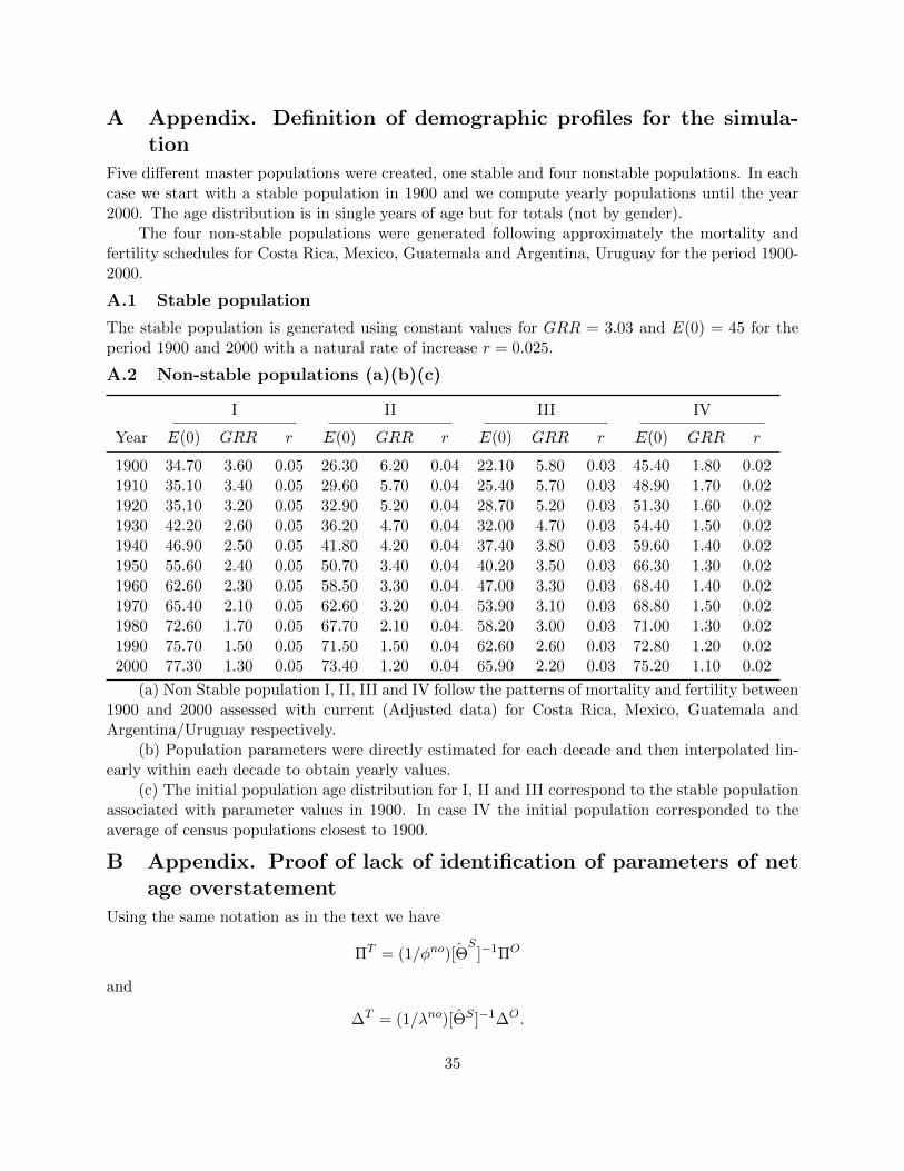
We first simulate a large number of populations spanning a broad range of fertility and mortalityregimes that come close to reproducing age-specific counts of deaths and populations that wouldhave been observed over an interval of about 100 years in the absence of errors in the data. Westart out with a stable age distribution in single years of age, e.g., Pxt0 , x = 0, ...100, to represent anaverage population in 1900 and then project it forward for 100 years using schedules of mortality,e.g. (Sx = 0, 100), and fertility, e.g., (Fx = 15, 50) 12. We chose four different trajectories ofmortality and fertility roughly reproducing four classes of demographic transitions experienced byArgentina, Costa Rica, Guatemala and Mexico respectively (Palloni, 1990). All four trajectoriesare defined by choosing values of life expectancy at birth (E0), and Gross Reproduction Rate(GRR) thus identifying the rate of natural increase (r) for every decade between 1900 and 2000.With the exception of the first trajectory (corresponding to the experiences of Argentina andUruguay), we assume an initial stable populations with r and E0 equal to those observed in thefirst population census before 1940 for each trajectory. In the case of the Argentina/Uruguayprofile we use the observed average age distribution in the population censuses within the period1850-1910. We assume linear intra-decade changes in the two key population parameters, r and
10The investigations that follow were first documented elsewhere (Palloni and Pinto, 2000)11Hill and colleagues did consider simulations that included limited forms of age misreporting. We augment this
aspect to capture patterns of age misreporting typically observed in LAC countries as well as the performance of anew method to adjust for associated errors.
12Throughout we use conventional mathematical notation and when referring to discrete functions we employsubscripts, e.g. Px, whereas for continuous functions we use the parentheses enclosing the function’s argument, e.g.P(x).
19
E0 and, additionally, that each type of demographic transition profile preserves the age patterns ofmortality and fertility. We chose the West model in the Coale-Demeny family of life tables and anage pattern of fertility identical to the one used in the computations of the Coale-Demeny stablepopulation models (Coale et al., 1983). Information on the four classes of demographic transitionsused here are in Appendix A. Finally, we construct a fifth profile of a stable population with naturalrate of increase and fertility pattern equivalent to the average of LAC populations in the interval1950-60, e.g. not yet heavily perturbed by large scale net migration as is the case in Argentina,Brazil, Cuba, and Uruguay, or early fertility changes, as in Argentina and Uruguay.
Following routine population projection calculations we produce 505 populations and asso-ciated distributions of births and deaths by single calendar year and single years of age. Thesimulated populations represent a very broad set of experiences, from those preserving populationstability up until 1950 or thereabouts, to those shifting to quasi-stability from 1930 up to 1980, tothose with little or no stability at all from the start13.
5.2 Simulated distortions I: imperfect relative completeness of death registra-tion
Distortions due to population or death coverage can be implemented in a straightforward matter.We define observed population (or death) counts by age as a fraction of the simulated (true)quantities:
P oxt1 = C1Psxt1
P oxt2 = C2Psxt2 ; t2 < t1
Doxt = C3D
sxt; t = t1, t1 + 1, ... ≤ t2
for x ≥ 5, where P oxt1 is the observed (distorted) population at age (x, x + 1] at time t1, Poxt2 is
the observed (distorted) population at age (x, x+ 1] at time t2, and Doxt is the observed (distorted)
number of deaths in year t; P sxt1 , Psxt2 and Ds
xt are the simulated (true) quantities and C1, C2 andC3 are the fractions of total events actually observed (completeness factors). The completenessfactors for censuses were set at values in the range 0.80-1.0 in intervals of 0.5 whereas the deathcompleteness factors varied between 0.70 and 1.0 in intervals of 0.5. Altogether we produce a totalof 875 (175*5) patterns of including distorted and true demographic profiles. These definitions aresufficient to evaluate adjustment methods that require only one census and one to three years ofdeath counts centered on the census or, alternatively, those that demand as inputs two populationcensuses and an array of intercensal deaths.
The above set up contains a massive assumption, namely, that completeness of both populationand death counts is age invariant. At least within the age range in which the techniques are deployed(5-85), the assumption is unlikely to be met, particularly for population counts. To complete theset of reasonable distortions we add two different patterns of age varying completeness generatinga total of 2,625 simulated populations. We show later, however, that as long as the differencebetween maximum and minimum completeness stays below 10% of the mean value of completeness,the variance of completeness by age does not have a strong impact on choices of techniques (Section6).
13To compute single years of age stable populations we first generate single years of age life tables by respecting theseparator factors adopted by Coale and Demeny and the use of standard stable population expressions. The preciseroutine followed is in a STATA do file available on request from authors.
20
5.3 Simulated distortions III: combining age misreporting and faulty coverage
We now have all the ingredients to generate distorted populations using as benchmarks the demo-graphic profiles described above. The defective populations were defined considering each demo-graphic profile separately, letting C1 and C2 take on values between 0.80 and 1.0 in intervals of0.05 whereas C3 takes on values between 0.75 and 1.0 in intervals of 0.05 and, finally, assigningvalues to φno and λno ranging from 0 to 2.5 in intervals of 0.50. We use all possible combinationsof these parameters and generate a total of 6,300 populations per demographic profile (5 in all) fora population space containing a total of 31,500 observations or populations in single years of agetraced for a total of 100 years. In addition, to test for sensitivity to violations of the assumptionof age invariant relative completeness, we add two patterns of deviations and generate a space of94,500 populations.
5.4 Application of adjustment techniques
The next stage in the evaluation is to apply the 11 techniques to adjust for defective completenessas well as the technique developed above to correct for age misreporting.
5.4.1 Techniques to adjust for defective completeness
The most important techniques to detect and adjust for faulty completeness evaluated in this studyare summarized in Table 814. The table identifies techniques using the names of researcher(s) whoproposed them or modified an original version. The table highlights (a) key assumptions on whichthe techniques rely, and (b) information required to implement each of them. These methods shareimportant commonalities and all but two (Brass No 1 and Preston-Hill No 1) abstain from invokingthe assumption of stability. Yet they differ in at least one feature that, under suitable empiricalconditions, grants them an advantage over competing methods.
The key features of these techniques are the following:
• Computation of rates of growth: with two exceptions (Preston-Hill No1 and Brass) all meth-ods require computation of age specific rates of growth in an intercensal period. Becauseobserved rates may be perturbed by differential census completeness, the estimates of themain parameter (relative completeness of death registration) could be biased if the method issensitive to differential census completeness. A way around this is to first adjust for relativecompleteness of census registration and then apply any of the techniques using adjusted agespecific rates of growth. This idea was first put forward by Hill (Hill and Choi, 2004; Hillet al., 2009) who suggests that one of the methods listed in the table (Brass-Hill) be used toretrieve a robust estimate of the ratio of completeness of both censuses.
• Population closed to migration: none of the methods in Table 8 works well in the presenceof significant intercensal migration. If information on net migration is available, it must beused to adjust the observed rates of intercensal growth15
• Absence of age misreporting: all methods assume either no age misreporting or, alternatively,age misreporting that perturbs only trivially the figures of cumulative population above adult
14We reviewed a longer list of techniques and, with two exceptions, chose to test only those that did not rely onthe assumption of stability or quasi-stability.
15Hill and colleagues investigated the effects of intercensal migration (Hill et al., 2009). In the simulations performedhere we do not include consideration of migration but its effects are partially captured via differential censusescompleteness.
21
Table 8: Methods to adjust for completeness of death registration: assumptions and required data.
Method Assumptions Required Data
Brass (B) 1-2-3-4-5 BBrass-Hill (BHill2) 2-3-4 ABrass-Martin (BMartin3) 1-2-3-4-6 BBennet-Horiuchi No 1 (BH 1) 1-2-3-4 ABennet-Horiuchi No 2 (BH 2) 1-2-3-4 ABennet-Horicuhi No 3 (BH 3) 1-2-3-4 ABennet-Horiuchi No 4 (BH 4) 1-2-3-4 ABennet-Horiuchi No 5 (2SBH 4) 1-2-3-4 APreston-Hill No 1 (PH 1) 1-2-3-4-5 BPreston-Hill No 2 (PH 2) 1-2-3-4 APreston-Bennet (PB) 1-2-3-4 APreston-Lahiri No 1 (PL 1) 1-2-3-4 APreston-Lahiri No 2 (PL 2) 1-2-3-4 A
1See appendix 5 for definitions of the four variants of Bennet-Horiuchi method and the two variantsof Preston-Lahiri method.2BHill is a method we use to retrieve estimates of the ratio of completeness of the first relative tothe second census.3BMartin is a variant of Brass classic method that relaxes the assumption of stability and assumesinstead past mortality decline.
KEYS FOR ASSUMPTIONS1. Identical completeness of census counts in both census2. Closed to migration3. No age misreporting4. Invariant completeness by age5. Stability6. Quasi stability
KEYS FOR REQUIRED DATAA. Two censuses and intercensal deathsB. One census and one to three years of deaths by age
22
ages. This poses a conundrum: if, as asserted before, LAC population and mortality countsare heavily affected by age overstatement, how can one expect to obtain precise estimates ofrelative completeness using techniques that are vulnerable when there is age misreporting?There are two conditions that provide a escape from this trap. The first is that the type of agemisreporting that predominates in LAC is net age overstatement. When using cumulativepopulations over some age x the damage done to the target quantity by age misreportingonly depends on population flows across age x originating at younger ages. It is insensitiveto transfers of population above age x. Furthermore, the relative volume of flows, e.g. therelative error of the target quantity, is generally low for late adulthood and early old ages (lessthan 65 or 70) though it begins to mount after age 75 or so. Since in all cases computationsonly require to employ observations up to ages 70 or 75, the impact of age overstatement willbe minor16.The second favorable condition that circumvents the problem is that the optimalmethod (Bennett-Horiuchi No 4) is also the least sensitive to age misreporting of the typeencountered in LAC (see below).
• Age invariant relative completeness of death registration: all techniques rely on the assump-tion that the relative completeness of death registration is age invariant. However, as weshow later, when there are mild violations of the assumption the optimal method we choose(Bennett-Horiuchi IV) performs best.
• Estimation of life expectancy at older ages: all methods adopt ad hoc procedures to handlethe open age group. These procedures rely on exogenous computations of parameters relatingthe quantity of interest, life expectancy at age 75 or 70 and selected observed quantities inthe data at hand. The relations are estimated using model life tables, stable populationexpressions, numerical approximations or a combinations of all these. In the applicationsimplemented here we follow the methods suggested by the authors in each case. Thus, someof the variability in performance that we uncover, albeit a small part, is due to heterogeneousstrategies to handle the open age group.
5.4.2 Techniques to adjust for age misreporting
We consider only one technique to adjust the observed data for age misreporting. As describedbefore, the procedure rests on two key assumptions. The first is that errors follow a known agepattern (the Costa Rican standard). The second is the age pattern of age misreporting is the samein the census and in vital statistics. both are simplification and a more comprehensive evaluationstudy should include deviant patterns.
6 Results of the evaluation study
We now review results of applying candidate techniques for adjusting defective relative completenessand age misreporting. We base our discussion on results from the set of simulated populationsdescribe before, a space of fictitious populations and deaths generated by five different demographicregimes combined with an exhaustive set of error patterns. In section 6.1 we describe the behaviorof these techniques, that is, their effectiveness to retrieve population parameters under severalconditions: ignoring the error patterns embedded in the space of simulated populations, in subsets
16This is because even with heavy age overstatement the population at any particular age y < x, where x is below65 or so, is a small fraction of the population above age x. These ratios increase as x increases due to exponentialdecrease of population at older ages.
23
of populations defined by selected underlying conditions and, finally, isolating two types of errorsthat violate basic assumptions of all methods considered here, namely, age misreporting and agedependent completeness. In section 6.2 we describe the behavior of methods to adjust for agemisreporting.
6.1 Defective completeness: evaluation using pooled simulated populations
To facilitate assessment of techniques we create six different populations subsets: (a) total orpooled, (b) stable, (c) non-stable, (d) non-stable with no age misreporting, with defective death andpopulation coverage, (e) non-stable with age misreporting, incomplete death coverage and defectivebut identical population coverage in the two censuses and (f) non-stable with age misreporting,incomplete death and population coverage. Each subpopulation with incomplete population and/ordeath coverage has three variants, one with constant relative completeness (of census and deathscounts) and the others with age varying completeness.
Investigating the behavior of techniques isolating conditions that generate errors is helpfulwhen there is reliable external information about population stability, nature of age misreportingand/or patterns of age relative completeness. A technique that performs optimally in the pooledsimulated population may not do so well under a specific set of conditions. The opposite situation isalso possible: a technique may not behave well on average but could be optimal under some circum-stances. Because the source of uncertainty matters for the final choice of method, our assessment iscarried out across multiple subsets of simulated populations, each reflecting different types of errorsor conditions. We define the following six population subsets: a) pooled sample (n=31,500), b) sta-ble populations (n=6,300), c) non-stable populations (n=25,200), d) non-stable populations withno age misreporting but defective completeness of death and population counts (n=700) e) non-stable populations with age misreporting, defective coverage of death counts and equal (possibledefective) coverage of population counts (n=4,320) and, finally, f) non-stable population with agemisreporting, defective death registration, defective (but unequal) population counts (n=17,280).In each of these subsets we generate three variants, one assuming constant relative completenessand two variants imposing two different age-dependent patterns of relative completeness17.
We evaluate the following techniques: Brass technique (Brass, 1975) modified by Hill (Hill,1987) to compute a robust estimate of relative completeness in two population censuses and 11techniques to estimate relative completeness of death registration: a) original Brass method (Brass,1975) modified by Hill (Hill, 1987) and variant by Martin (Martin, 1980), b) four variants of Bennettand Horiuchi (Bennett and Horiuchi, 1981;1984), c) one method by Preston and Bennett (Prestonand Bennett, 1983), d) two different methods by Preston and Hill (Preston and Hill, 1980), and e)two variants of Preston and Lahiri (Preston and Lahiri, 1991).
The assessment focuses on the mean proportionate (absolute) errors for two population pa-rameters, the ratio of completeness of first to second census coverage, ρc=C1/C2 and the relativecompleteness of death registration, ρd = (C3/(.5 ∗ (C1 + C2)). Tables 9–11, panels A throughpanel F display the mean of the proportionate absolute error for each of the six populations sub-sets defined above. The errors in each population subset s, s = 1, 2...6, are Ξd
s =∑j=Ks
j=1 εdsj and
Ξcs =
∑j=Ksj=1 εcsj where εdsj =| ρdsj−ρdsj | /ρdsj , εcsj =| ρcsj−ρcsj | /ρsj , ρc and ρd are defined as before,
ρdsj and ρcsj are estimates, and the summations are over all simulated populations j in each of six
17The two functions for age dependent census completeness are assumed to hold in both censuses and are definedas follows: (a) scenario 1: C1= 0.75 if age [15-34] and C1= 0.85 elsewhere; C2=0.85 if age [15-34] and C2= 0.95elsewhere; C3= 0.80 if age [15-34] and C3= 0.85 elsewhere; (b) scenario 2: C1= 0.85 if age [15-34] and C1= 0.75elsewhere; C2= 0.95 if age [15-34] and C2= 0.85 elsewhere; C3= 0.85 if age [15-34] and C3= 0.80 elsewhere.
24
subsets. Naturally, different error metrics yield different ranking of methods but the measure weuse is the preferred one in most applications of this kind.18
The six panels of Tables 9–11 display the mean of the proportionate absolute error for eachof the six populations subsets defined above. Table 9 refers to simulations with constant relativecompleteness by age and Tables 10 and 11 reflect results using two different patterns of age varyingrelative relative completeness. The errors in each population subset s, s = 1, 2...6, are Ξd
s =∑j=Ksj=1 εdsj and Ξc
s =∑j=Ks
j=1 εcsj , where εdsj =| ρdsj − ρdsj | /ρdsj , εcsj =| ρcsj − ρcsj | /ρsj , ρc and ρd are
defined as before, ρdsj and ρcsj are estimates, and the summations are over all simulated populationsj in each of six subsets. Naturally, different error metrics yield different ranking of methods butthe measure we use is the preferred one in most applications of this kind19.
18The figures in Tables 9–11, panel A through panel F are computed using a subset of rather benign patterns ofdistortions as they exclude values of completeness lower than 0.7 and differences between completeness of successivecensuses higher than 0.10.
19We emphasize that the figures in Tables 9–11, are computed on a subset of rather benign patterns of distortionsas they exclude values of relative completeness lower than 0.7 and differences between completeness of successivecensuses higher than 0.10.
25
Tab
le9:
Pro
port
ion
ate
abso
lute
erro
rsin
each
ofsi
xp
opu
lati
ons
sub
sets
wit
hage
inva
riant
rela
tive
com
ple
ten
ess.
A.
Sta
ble
&N
onst
ab
eB
.Sta
ble
C.
Nonst
able
D.
Nonst
able
?E
.N
onst
able•
F.
Nonst
able‡
Indic
ato
rM
ed
Mean
SD
Med
Mean
SD
Med
Mean
SD
Med
Mean
SD
Med
Mean
SD
Med
Mean
SD
Bra
ssH
ill
Censu
s(B
Hill)1
0.0
03
0.0
03
0.0
03
0.0
05
0.0
05
0.0
04
0.0
03
0.0
03
0.0
02
0.0
01
0.0
01
0.0
01
0.0
02
0.0
03
0.0
02
0.0
02
0.0
03
0.0
02
Bennet
Hori
uchi
No
1(B
H1)
0.2
42
0.3
04
0.2
65
0.1
99
0.2
63
0.2
24
0.2
51
0.3
14
0.2
73
0.2
15
0.2
94
0.2
51
0.0
10
0.0
14
0.0
11
0.2
12
0.2
56
0.1
17
Bennet-
Hori
uchi
No
2(B
H2)
0.2
48
0.3
00
0.2
56
0.2
15
0.2
60
0.2
16
0.2
60
0.3
10
0.2
64
0.2
15
0.2
96
0.2
53
0.0
11
0.0
13
0.0
10
0.2
19
0.2
56
0.1
11
Bennet-
Hori
cuhi
No
3(B
H3)
0.2
40
0.3
03
0.2
63
0.2
00
0.2
64
0.2
25
0.2
47
0.3
12
0.2
71
0.2
12
0.2
93
0.2
49
0.0
10
0.0
13
0.0
11
0.2
10
0.2
55
0.1
15
Bennet-
Hori
uchi
No
4(B
H4)
0.2
48
0.3
00
0.2
56
0.2
15
0.2
60
0.2
16
0.2
60
0.3
10
0.2
64
0.2
15
0.2
96
0.2
53
0.0
11
0.0
13
0.0
10
0.2
19
0.2
56
0.1
11
Bennet-
Hori
uchi
No
5(2
SB
H4)
0.0
21
0.0
24
0.0
17
0.0
16
0.0
20
0.0
15
0.0
23
0.0
25
0.0
17
0.0
07
0.0
08
0.0
05
0.0
22
0.0
24
0.0
16
0.0
23
0.0
25
0.0
17
Bra
ss-M
art
in(B
Mart
in)2
0.0
79
0.1
07
0.0
85
0.0
38
0.0
38
0.0
21
0.1
10
0.1
24
0.0
86
0.0
57
0.0
71
0.0
61
0.1
12
0.1
24
0.0
84
0.1
11
0.1
24
0.0
85
Bra
ssH
ill
(BH
ill)
10.0
43
0.0
46
0.0
27
0.0
38
0.0
38
0.0
21
0.0
45
0.0
48
0.0
28
0.0
05
0.0
06
0.0
04
0.0
45
0.0
48
0.0
28
0.0
45
0.0
48
0.0
28
Pre
ston
Bennet
(PB
)0.6
29
0.7
28
0.5
52
0.4
93
0.6
23
0.5
94
0.7
01
0.7
54
0.5
37
0.5
81
0.6
92
0.5
41
0.0
31
0.0
51
0.0
49
0.6
29
0.8
53
0.5
10
Pre
ston
Hil
lI
(PH
1)
0.3
40
0.3
88
0.2
97
0.2
75
0.3
81
0.3
75
0.3
56
0.3
90
0.2
74
0.3
58
0.3
88
0.2
67
0.2
03
0.2
26
0.1
46
0.3
25
0.3
08
0.1
75
Pre
ston-H
ill
2(P
H2)
0.3
67
0.3
86
0.2
72
0.2
49
0.3
67
0.3
20
0.3
74
0.3
91
0.2
58
0.3
77
0.3
90
0.2
51
0.2
42
0.2
58
0.1
46
0.3
48
0.3
15
0.1
81
Pre
ston
Lahir
iN
o1
(PL
1)
0.4
06
5.9
11
260.8
80
0.3
36
1.4
98
4.4
78
0.4
49
7.0
14
291.6
55
0.4
52
3.4
34
20.6
99
0.0
21
0.0
23
0.0
15
0.4
23
11.1
92
451.1
44
Pre
ston-L
ahir
iN
o2(P
L2)
0.3
78
5.5
60
168.4
22
0.3
07
1.3
66
4.5
58
0.4
15
6.6
09
188.2
74
0.4
14
2.0
64
6.9
47
0.0
22
0.0
27
0.0
21
0.3
94
0.9
16
3.4
22
N31,5
00
6,3
00
25,2
00
700
4,3
20
10,3
68
SD
,st
andard
devia
tion;
Med,
media
n.
?θ1
=θ3
=0
•C
1=C
2andC
3<
1‡C
16=C
2andC
3<
1and
maxabs(C
1−C
2)<.1
01V
alu
es
of
err
ors
inth
eB
rass
-Hill
show
nin
the
firs
tro
wcorr
esp
ond
toerr
ors
ass
ocia
ted
wit
hth
era
tioC
1/C
2.
While
valu
es
of
Bra
ss-H
ill
inth
ese
venth
row
corr
esp
ond
toerr
os
ass
ocia
ted
wit
hre
lati
ve
com
ple
teness
of
death
regis
trati
on.
2B
Mart
inis
avari
ant
of
Bra
sscla
ssic
meth
od
that
rela
xes
the
ass
um
pti
on
of
stabil
ity
and
ass
um
es
inst
ead
past
mort
ality
decline.
26
Tab
le10
:P
rop
orti
on
ate
ab
solu
teer
rors
inea
chof
six
pop
ula
tion
ssu
bse
tsw
ith
age
dep
end
ent
rela
tive
com
ple
ten
ess
(Sce
nari
o1).
A.
Sta
ble
and
Nonst
ab
eB
.Sta
ble
C.
Nonst
able
D.
Nonst
able
?E
.N
onst
able•
F.
Nonst
able‡
Indic
ato
rM
ed
Mean
SD
Med
Mean
SD
Med
Mean
SD
Med
Mean
SD
Med
Mean
SD
Med
Mean
SD
Bra
ssH
ill
Censu
s(B
Hill)1
0.0
40
0.0
46
0.0
33
0.0
39
0.0
45
0.0
32
0.0
40
0.0
47
0.0
33
0.0
39
0.0
45
0.0
32
0.0
13
0.0
15
0.0
10
0.0
38
0.0
37
0.0
20
Bennet
Hori
uchi
No
1(B
H1)
0.2
67
0.3
19
0.2
79
0.2
73
0.3
31
0.2
96
0.2
65
0.3
16
0.2
75
0.2
17
0.2
95
0.2
53
0.0
16
0.0
20
0.0
18
0.2
08
0.2
56
0.1
25
Bennet-
Hori
uchi
No
2(B
H2)
0.2
67
0.3
15
0.2
69
0.2
71
0.3
27
0.2
85
0.2
65
0.3
12
0.2
64
0.2
17
0.2
97
0.2
54
0.0
19
0.0
23
0.0
19
0.2
15
0.2
55
0.1
16
Bennet-
Hori
cuhi
No
3(B
H3)
0.2
67
0.3
17
0.2
77
0.2
72
0.3
29
0.2
93
0.2
63
0.3
14
0.2
72
0.2
14
0.2
94
0.2
51
0.0
17
0.0
21
0.0
18
0.2
05
0.2
55
0.1
23
Bennet-
Hori
uchi
No
4(B
H4)
0.2
67
0.3
15
0.2
69
0.2
71
0.3
27
0.2
85
0.2
65
0.3
12
0.2
64
0.2
17
0.2
97
0.2
54
0.0
19
0.0
23
0.0
19
0.2
15
0.2
55
0.1
16
Bennet-
Hori
uchi
No
5(2
SB
H4)
0.0
99
0.1
50
0.3
50
0.1
47
0.3
32
0.7
37
0.0
88
0.1
05
0.0
81
0.0
78
0.0
92
0.0
68
0.0
30
0.0
33
0.0
23
0.0
82
0.0
85
0.0
52
Bra
ss-M
art
in(B
Mart
in)2
0.1
62
0.2
59
0.2
92
0.1
54
0.2
09
0.1
85
0.1
64
0.2
71
0.3
12
0.1
41
0.2
07
0.2
17
0.1
61
0.1
70
0.1
04
0.1
29
0.2
12
0.2
11
Bra
ssH
ill
(BH
ill)
10.1
19
0.1
62
0.1
51
0.1
20
0.1
57
0.1
39
0.1
18
0.1
63
0.1
54
0.1
02
0.1
28
0.1
09
0.0
78
0.0
81
0.0
43
0.0
96
0.1
24
0.1
03
Pre
ston
Bennet
(PB
)0.7
42
0.7
28
0.3
88
0.7
90
0.7
84
0.3
46
0.7
29
0.7
14
0.3
96
0.5
49
0.5
94
0.4
08
0.1
86
0.2
07
0.1
46
0.7
03
0.7
66
0.3
73
Pre
ston
Hill
I(P
H1)
0.4
45
0.5
14
0.4
46
0.4
44
0.5
14
0.4
48
0.4
47
0.5
14
0.4
45
0.4
47
0.5
08
0.4
32
0.2
24
0.2
47
0.1
45
0.4
01
0.3
72
0.2
09
Pre
ston-H
ill
2(P
H2)
0.4
56
0.5
05
0.4
15
0.4
59
0.5
04
0.4
17
0.4
32
0.5
06
0.4
15
0.4
50
0.5
00
0.4
01
0.2
60
0.2
77
0.1
45
0.4
31
0.3
68
0.2
16
Pre
ston
Lahir
iN
o1
(PL
1)
0.5
41
6.4
32
507.3
47
0.5
38
1.9
26
4.0
66
0.5
41
7.5
58
567.2
25
0.5
34
2.1
02
5.8
92
0.0
34
0.0
39
0.0
26
0.5
07
6.1
39
74.3
53
Pre
ston-L
ahir
iN
o2(P
L2)
0.4
77
6.5
82
256.1
06
0.4
39
1.4
24
2.2
06
0.4
81
7.8
72
286.3
20
0.4
82
2.5
09
11.8
76
0.0
44
0.0
51
0.0
35
0.4
52
1.6
05
3.4
91
N31,5
00
6,3
00
25,2
00
700
4,3
20
10,3
68
SD
,st
andard
devia
tion;
Med,
media
n.
?θ1
=θ3
=0
•C
1=C
2andC
3<
1‡C
16=C
2andC
3<
1and
maxabs(C
1−C
2)<.1
01V
alu
es
of
err
ors
inth
eB
rass
-Hill
show
nin
the
firs
tro
wcorr
esp
ond
toerr
ors
ass
ocia
ted
wit
hth
era
tioC
1/C
2.
While
valu
es
of
Bra
ss-H
ill
inth
ese
venth
row
corr
esp
ond
toerr
os
ass
ocia
ted
wit
hre
lati
ve
com
ple
teness
of
death
regis
trati
on.
2B
Mart
inis
avari
ant
of
Bra
sscla
ssic
meth
od
that
rela
xes
the
ass
um
pti
on
of
stabil
ity
and
ass
um
es
inst
ead
past
mort
ality
decline.
Scenari
o1:C
1=
0.7
5if
age
[15-3
5],C
1=
0.8
5els
ew
here
;C
2=
0.8
5if
age
[15-3
5],C
1=
0.9
5els
ew
here
;C
3=
0.8
0if
age
[15-3
5],C
1=
0.8
5els
ew
here
.
27
Tab
le11
:P
rop
orti
on
ate
ab
solu
teer
rors
inea
chof
six
pop
ula
tion
ssu
bse
tsw
ith
age
dep
end
ent
rela
tive
com
ple
ten
ess
(Sce
nari
o2).
A.
Sta
ble
and
Nonst
ab
eB
.Sta
ble
C.
Nonst
able
D.
Nonst
able
?E
.N
onst
able•
F.
Nonst
able‡
Indic
ato
rM
ed
Mean
SD
Med
Mean
SD
Med
Mean
SD
Med
Mean
SD
Med
Mean
SD
Med
Mean
SD
Bra
ssH
ill
Censu
s(B
Hill)1
0.0
41
0.0
45
0.0
31
0.0
42
0.0
46
0.0
31
0.0
41
0.0
45
0.0
31
0.0
43
0.0
46
0.0
31
0.0
29
0.0
30
0.0
10
0.0
33
0.0
36
0.0
28
Bennet
Hori
uchi
No
1(B
H1)
0.2
44
0.3
11
0.2
86
0.2
49
0.3
27
0.3
00
0.2
43
0.3
07
0.2
82
0.2
18
0.2
80
0.2
59
0.0
15
0.0
19
0.0
16
0.2
34
0.2
45
0.1
43
Bennet-
Hori
uchi
No
2(B
H2)
0.2
42
0.3
10
0.2
71
0.2
47
0.3
25
0.2
85
0.2
40
0.3
07
0.2
67
0.2
18
0.2
83
0.2
62
0.0
54
0.0
55
0.0
30
0.2
25
0.2
33
0.1
34
Bennet-
Hori
cuhi
No
3(B
H3)
0.2
44
0.3
09
0.2
84
0.2
49
0.3
24
0.2
97
0.2
43
0.3
05
0.2
80
0.2
15
0.2
78
0.2
57
0.0
14
0.0
18
0.0
15
0.2
33
0.2
44
0.1
40
Bennet-
Hori
uchi
No
4(B
H4)
0.2
42
0.3
10
0.2
71
0.2
47
0.3
25
0.2
85
0.2
40
0.3
07
0.2
67
0.2
18
0.2
83
0.2
62
0.0
54
0.0
55
0.0
30
0.2
25
0.2
33
0.1
34
Bennet-
Hori
uchi
No
5(2
SB
H4)
0.0
81
0.1
18
0.2
76
0.0
95
0.2
47
0.5
86
0.0
74
0.0
86
0.0
62
0.0
78
0.0
83
0.0
52
0.0
34
0.0
37
0.0
25
0.0
60
0.0
63
0.0
41
Bra
ss-M
art
in(B
Mart
in)2
0.1
14
0.1
54
0.1
55
0.1
09
0.1
24
0.0
89
0.1
16
0.1
62
0.1
67
0.1
05
0.1
34
0.1
18
0.0
57
0.0
72
0.0
55
0.0
91
0.1
24
0.1
13
Bra
ssH
ill
(BH
ill)
10.0
94
0.1
09
0.0
83
0.0
96
0.1
07
0.0
72
0.0
94
0.1
10
0.0
85
0.0
96
0.1
04
0.0
69
0.0
30
0.0
33
0.0
23
0.0
82
0.0
85
0.0
49
Pre
ston
Bennet
(PB
)0.7
24
0.7
01
0.3
70
0.7
65
0.7
39
0.3
71
0.7
10
0.6
91
0.3
69
0.5
32
0.5
64
0.4
09
0.1
03
0.1
89
0.2
35
0.7
61
0.7
85
0.2
67
Pre
ston
Hill
I(P
H1)
0.4
14
0.5
21
0.4
90
0.3
80
0.5
28
0.4
96
0.4
18
0.5
20
0.4
89
0.4
26
0.5
12
0.4
73
0.1
39
0.1
80
0.1
53
0.3
43
0.3
83
0.2
01
Pre
ston-H
ill
2(P
H2)
0.4
12
0.5
08
0.4
56
0.4
01
0.5
13
0.4
63
0.4
39
0.5
07
0.4
54
0.4
24
0.5
00
0.4
39
0.1
79
0.2
08
0.1
58
0.3
72
0.3
74
0.2
02
Pre
ston
Lahir
iN
o1
(PL
1)
0.4
86
35.5
50
4655.5
69
0.4
92
7.2
33
101.1
18
0.4
83
42.6
30
5204.8
35
0.4
87
7.2
01
69.9
95
0.1
48
0.1
55
0.0
66
0.4
78
4.7
90
78.0
60
Pre
ston-L
ahir
iN
o2(P
L2)
0.4
50
13.1
37
640.0
44
0.4
48
19.4
91
974.4
94
0.4
31
11.5
48
524.1
00
0.4
49
3.1
16
14.2
27
0.2
07
0.2
21
0.1
16
0.4
13
12.9
01
323.7
72
N31,5
00
6,3
00
25,2
00
700
4,3
20
10,3
68
SD
,st
andard
devia
tion;
Med,
media
n.
?θ1
=θ3
=0
•C
1=C
2andC
3<
1
‡C
16=C
2andC
3<
1and
maxabs(C
1−C
2)<.1
0
1V
alu
es
of
err
ors
inth
eB
rass
-Hill
show
nin
the
firs
tro
wcorr
esp
ond
toerr
ors
ass
ocia
ted
wit
hth
era
tioC
1/C
2.
While
valu
es
of
Bra
ss-H
ill
inth
ese
venth
row
corr
esp
ond
toerr
os
ass
ocia
ted
wit
h
rela
tive
com
ple
teness
of
death
regis
trati
on.
2B
Mart
inis
avari
ant
of
Bra
sscla
ssic
meth
od
that
rela
xes
the
ass
um
pti
on
of
stabil
ity
and
ass
um
es
inst
ead
past
mort
ality
decline.
Scenari
o2:C
1=
0.8
5if
age
[15-3
5],C
1=
0.7
5els
ew
here
;C
2=
0.9
5if
age
[15-3
5],C
1=
0.8
5els
ew
here
;C
3=
0.8
5if
age
[15-3
5],C
1=
0.8
0els
ew
here
.
28
Search for an optimal estimate is carried out considering all prior information available andthe following are general rules:
i. In the absence of any knowledge whatsoever about errors or deviations from stability, thesearch for best method should be concentrated on the pooled sample subset in Tables 9–11,panel A.
ii. When exogenous information suggests stability and not much else, the search should focuson the subset of stable populations in Tables 9–11, panel B. Instead, when there is priorempirical data confirming violation of stability, for example past shifts in fertility regime, butone can be agnostic about completeness and age misreporting, the search of optimal methodshould concentrate on the population subset in Tables 9–11, panel C.
iii. When in addition to lack of stability there is evidence of defective coverage of population anddeath counts but no suggestion of significant net age overstatement at adult ages, the searchshould shift to the subset in Tables 9–11, panel D.
iv. When the researcher suspect a scenario like in (iii) above but, in addition, there is evidence ofage misreporting, identification of optimal method should be done using Tables 9–11, panelE.
v. Finally, in cases scenario (iv) is most reasonable and one can establish that completeness oftwo censuses is (possibly) defective but equal in both censuses, identification of the optimalchoice must be done with Tables 9–11, panel F.
The results displayed in Tables 9–11, panels A through F contain a number of salient char-acteristics. First, as already suggested in the work by Hill and colleagues, Brass’s methods toestimate relative completeness of the two censuses is uniformly good, regardless of population sub-set. Second, with the exception of Brass methods, the magnitude of errors are larger when censuscoverage is defective as long as completeness is NOT the same in both censuses. This is becauseall methods except Brass’s rely on direct computations of age specific growth rates from the ob-served data, a quantity that will be in error when there is different coverage errors in two successivecensuses. Indeed, the performance of these methods improves substantially when there is accuratecensus coverage or, equivalently, when coverage is the same in both censuses (Table 9, panel D).Fourth, age misreporting affects the accuracy of all estimates but substantially more so in somecases (Brass’s methods and the second variant of Preston-Hill) than in others (Bennett-Horiuchi allvariants). Fifth, the magnitude of errors obtain when relative completeness is age dependent (lasttwo columns of panels A-F in Tables 9–10) varies sharply by technique but, in general, are lowestin the method by Bennett-Horiuchi.
The most important inference from this evaluation exercise is as follows: if one excludes popu-lation subsets with defective census completeness, the optimal choice is always one of the variants ofBennett-Horiuchi method followed by the two methods proposed by Brass, irrespective of violationsof stability assumptions or age misreporting. This suggests the following strategies:
i. In the absence of exogenous information about the difference in completeness between thetwo census and if the assumption of age invariant completeness holds, use Brass method;
ii. In the absence of exogenous information, whether or not age dependence of relative com-pleteness is suspected, use a two stage procedure: first estimate relative completeness of
29
census enumeration using Brass’ method, adjust intercensal rates of growth and then applyBennett-Horiuchi method.
We use both strategies in LAC and when the difference between estimates was less than 0.05 wecompute the average of Brass and Bennett Horiuchi estimates. When their difference exceeded 0.05we chose the estimate from strategy (ii)20.
6.2 Defective age reporting
Do the procedures to identify and adjust for age misreporting produce robust estimates of the truepopulation parameters? To answer this question we select the subset of simulated populationswith age misreporting and defective completeness, adjusted for completeness following strategy (ii)above, we identify the existence of age misreporting, and then correct for it using techniques (ii)in section 4.2. Tables 5 through 7 display the main results. First, Table 5 contains parametersassociated with expression (4.5) and reveals that the fit is almost perfect and that the estimatedconstant is unit, as it should be. Table 6 shows that when the procedure is reversed and we regresscmRx on the vectors α1x=45,100 and α2x=45,100 the errors of estimates are trifle. This suggests thatif an observed population belongs to the space of simulated populations, we can retrieve estimatesof the magnitude of age net over-reporting that are highly accurate by simply using the estimatedrelation between the observed cmRx and estimates α1x=45,100 and α2x=45,100 from the simulatedpopulations.
7 Discussion: the issue of uncertainty
By an large the methods to adjust mortality statistics reviewed here perform satisfactorily providedthe key assumptions on which they rest are concordant with the empirical conditions that producethe data. This is most unlikely to be the case always or even frequently for one single assumptionand much less for combinations of assumptions. The conventional strategy has invariably beento scrutinize alternative estimates and then settle for one based on explicit or, more frequently,implicit reasoning and judgments about concordance of assumptions and observables. We believewe can improve upon this practice.21
The evaluation study generates a superpopulation of errors associated with the applicationof each technique under conditions that violate to different degrees one or several of the cardinalassumptions on which they rely. It follows that for each technique we can define precisely themagnitude of error—however measured— associated with conditions that depart from the combi-nation of assumptions in ex ante known ways. In our simulation the base universe of populationswas generated by combining different demographic parameters (levels and patterns of fertility andmortality) thus producing multiple instances where one could alter conditions imparting changesthat violate assumptions(lack of stability, adult migration, variable completeness, age misreportingthat departs from assumed patterns etc.). As a consequence, we have all the information neededto define the frequency distribution of errors associated with one technique under one set of simu-lated conditions. And, in particular, one can define the probability that a singular technique will
20It is important to note that when relative completeness is age dependent, Bennett-Horiuchi is mean optimal,in the sense that the weighted average of relative death completeness of observed data will be best estimated byBennett-Horiuchi methods. It does not mean that, once applied, the adjusted mortality rates (and derived functionof the life table) will also be best estimates. None of the methods we include in our evaluation can escape from theassumption of constant relative completeness and, therefore, we can only aspire to find a mean optimal candidate.
21An application of the ideas described here is in Palloni and Beltran-Sanchez (2016).
30
produce an error less than, say 5, percent under a given set of well defined (simulated) conditionsthat possibly depart from assumptions.
Now, assume that in any population we know the probability that the historical conditionsthat produced the data match one of the multiple sets of simulated conditions.22 It would thenbe possible to compute the unconditional probability that, in that particular population, a giventechnique will produce an error of less than 5 percent. If one repeats this for all candidate techniquesthan can be deployed, we will have alternative values of the true parameters and known magnitudeof uncertainty associated with each of them. This is sufficient knowledge to analyze the dataincorporating uncertainty-rather than ignoring it by a sleigh of hand choosing the value discerned,however convincingly, to be the true parameter. The outcome of this is that target parameters suchas the rate of decline of mortality rates for a given age group, the effects of income on mortalitychanges, the fraction of life expectancy improvements associated with income changes, will beassociated with bounds of uncertainty and the standard errors of these estimates will fall within arange rather than being point estimates. This may be less pleasing than providing a single value(with associated standard errors) but it is also a strategy that fully admits levels of ignorance.Since some of the estimates could be used for projections and forecasts, it stands to reason thatthe above procedure will lead to probabilistic forecasts by virtue of uncertainty of estimates notjust because of uncertainty about future trends.
22These probabilities can be constructed from expert judgments.
31
References
Bhat, M. P. (1987), “Mortality in India: Levels, Trends and Patterns,” Ph.d., University of Penn-sylvania.
Bhat, P. N. M. (1990), “Estimating Transition Probabilities of Age Misstatement,” Demography,27, 149–163.
Brass, W. (1975), Methods for Estimating Fertility and Mortality from Limited and Defective Data:based on seminars held 16-24 September 1971 at the Centro Latinoamericano de Demografıa(CELADE) San Jose, Costa Rica, Chapel Hill, NC: International Program of Laboratories forPopulation Statistics, Dept. of Biostatistics, School of Public Health, Carolina Population Center,Univ. of North Carolina at Chapel Hill.
Chidambaram, V. and Sathar, Z. (1984), “Age and date reporting,” in Comparative Studies: Cross-National Summaries, Voorburg, Netherlands: International Statistical Institute, vol. 5.
Coale, A. J., Demeny, P., and Vaughan, B. (1983), “West? Model Life Tables and Stable Popula-tions,” in Regional Model Life Tables and Stable Populations (Second Edition), ed. Vaughan, A.J. C. D., Academic Press, pp. 41–154.
Coale, A. J. and Kisker, E. E. (1986), “Mortality Crossovers: Reality or Bad Data?” PopulationStudies, 40, 389–401.
Condran, G. A., Himes, C., and Preston, S. H. (1991), “Old-Age Mortality Patterns in Low Mor-tality Countries: An Evaluation of Population and Death Data at Advanced Ages, 1950 to thePresent,” Population Bulletin of the United Nations, 30, 23–60.
Dechter, A. R. and Preston, S. H. (1991), “Age misreporting and its effects on adult mortalityestimates in Latin America,” Popul Bull UN, 31-32, 1–16.
Del Popolo, F. (2000), “Los Problemas en la Declaracion de la Edad de la Poblacion Adulta Mayoren los Censos,” Report, CELADE, CEPAL, ECLAC.
Elo, I. T. and Preston, S. H. (1994), “Estimating African-American Mortality from InaccurateData,” Demography, 31, 427–458.
Ewbank, D. C. (1981), Age Misreporting and age-selection and Remuneration: Sources, Patterns,and Consequences for Demographics Analysis, Committee on Population and Demography, Wash-ington DC: National Reserach Coucil.
Grushka, C. O. (1996), “Adult and old age mortality in Latin America: Evaluation, adjustmentsand a debate over a distinct pattern,” Thesis, University of Pennsylvania.
Hill, K. (1987), “Estimating Census and Death Registration Completeness,” Asian and PacificPopulation Forum, 1, 8,23–13,24.
— (2003), “Adult mortality in the developing world: what we know and how we know it,” .
Hill, K. and Choi, Y. (2004), “Performance of GGB and SEG given various simulated data errors,”.
32
Hill, K., Choi, Y., and Timaeus, I. (2005), “Unconventional approaches to mortality estimation,”Demographic Research, S4, 281–300.
Hill, K., You, D., and Choi, Y. (2009), “Death distribution methods for estimating adult mortality:Sensitivity analysis with simulated data errors,” Demographic Research, 21, 235–254.
Horiuchi, S. and Coale, A. J. (1985), “Age Patterns of Mortality for Older Women,” .
Kamps E., J. (1976), La declaracion de la edad en los Censos de Poblacion de la America Latina;exactitud y preferencia de dıgitos en los Censos de 1950, 1960 y 1970, vol. Serie C of SeriesHistoricas, San Jose, Costa Rica: ONU, CEPAL, CELADE.
Martin, L. (1980), “A Modificationfor Use in Destabilized Populations of Brass’s Technqiue forEstimating Completeness of Death Registration,” Population Studies, 34, 381–95.
Mazess, R. B. and Forman, S. H. (1979), “Longevity and age exaggeration in Vilcabamba, Ecuador,”J Gerontol, 34, 94–8.
Nunez, L. (1984), “Una Aproximacion al Efecto de la Mala Declaracion de la Edad en la InformacionDemografica Recabada en Mexico,” Report, Direccion General del Registro Nacional de Poblacione Identificacion Personal.
Ortega, A. and Garcia, V. (1985), “Estudio Sobre la Mortalidad y Algunas Caracteristicas So-cioeconomicas de las Personas de la Tercera Edad: Informe de la Investigacion Efectuada en losCantones de Puriscal y Coronado del 3 al 20 de Junio de 1985,” Report, CELADE.
Palloni, A. (1990), “Assessing the Levels and Impact of Mortality in Crisis Situations,” in Mea-surement and Analysis of Mortality: New Approaches, eds. Vallin, J., D’Souza, S., and Palloni,A., New York: Oxford University Press, pp. 215–49.
Palloni, A. and Beltran-Sanchez, H. (2016), “Uncertainty and Mortality Estimates in the LatinAmerican and Caribbean (LAC) Region: 1850–2010,” working paper.
Palloni, A. and Pinto, G. (2000), “Fertility patterns and change in Latin America,” .
— (2004), “One hundred years of mortality in Latin America and the Caribbean: the fragile pathfrom hunger to longevity,” Presented at the annual meeting of the Population Association ofAmerica, Boston, Massachusetts, April 1-3, 2004.
Preston, S. and Hill, K. (1980), “Estimating the Completeness of Death Registration,” PopulationStudies, 34, 349–366.
Preston, S. H. and Bennett, N. G. (1983), “A Census-based Method for Estimating Adult Mortal-ity,” Population Studies, 37, 91–104.
Preston, S. H., Elo, I. T., Rosenwaike, I., and Hill, M. (1996), “African-American mortality at olderages: results of a matching study,” Demography, 33, 193–209.
Preston, S. H., Elo, T. I., Hill, M. E., and Rosenwaike, I. (2003), The Demography of AfricanAmericans, 1930-1990, Boston: Kluwer Academic Publishers.
33
Preston, S. H. and Lahiri, S. (1991), “A short-cut method for estimating death registration com-pleteness in destabilized populations,” Math Popul Stud, 3, 39–51.
Rosenwaike, I. (1987), “Mortality Differentials among Persons Born in Cuba, Mexico and PuertoRico Residing in the United States, 1979-81,” American Journal of Public Health, 77, 603–606.
Rosenwaike, I. and Preston, S. H. (1984), “Age Overstatement and Puerto Rican Longevity,”Human Biology, 56, 503–525.
Spencer, G. (1984), “Mortality among the Elderly Spanish Surnamed Population in the MedicareFiles: 1968 to 1979,” .
34
A Appendix. Definition of demographic profiles for the simula-tion
Five different master populations were created, one stable and four nonstable populations. In eachcase we start with a stable population in 1900 and we compute yearly populations until the year2000. The age distribution is in single years of age but for totals (not by gender).
The four non-stable populations were generated following approximately the mortality andfertility schedules for Costa Rica, Mexico, Guatemala and Argentina, Uruguay for the period 1900-2000.
A.1 Stable population
The stable population is generated using constant values for GRR = 3.03 and E(0) = 45 for theperiod 1900 and 2000 with a natural rate of increase r = 0.025.
(a) Non Stable population I, II, III and IV follow the patterns of mortality and fertility between1900 and 2000 assessed with current (Adjusted data) for Costa Rica, Mexico, Guatemala andArgentina/Uruguay respectively.
(b) Population parameters were directly estimated for each decade and then interpolated lin-early within each decade to obtain yearly values.
(c) The initial population age distribution for I, II and III correspond to the stable populationassociated with parameter values in 1900. In case IV the initial population corresponded to theaverage of census populations closest to 1900.
B Appendix. Proof of lack of identification of parameters of netage overstatement
Using the same notation as in the text we have
ΠT = (1/φno) ˆ[ΘS
]−1ΠO
and
∆T = (1/λno)[ΘS ]−1∆O.
35
In a closed population the relation between the vectors for populations in two successive cen-suses and the vector of intercensal deaths is:
ΠTt+k = ΠT
t + ∆T[t,t+k] . (B.1)
Using the first two expressions in (B.1) yields:
(1/φno) ˆ[ΘS
]−1ΠOt+k = (1/φno) ˆ[Θ
S]−1ΠO
t − (1/λno)[ΘS ]−1∆O[t,t+k] . (B.2)
From (B.2) we see that only (φno/λno) is identifiable with the available information.
C Appendix. Behavior of the age misreporting index cmRox,[t1,t2]
The expression of the age misreporting index is
cmRox,[t1,t2] =cmP ox+k,t2/cmP
ox,t1
1− (cmDox,[t1,t2]
/cmP ox,t1)
a ratio of two different estimators of the same quantity, namely the cumulative probability ofsurvival of the population aged x and over at time t1 to age (x + k) and over at time t2. Use ofcumulative quantities in the index is an important prerequisite since it minimizes the impact ofage misreporting within the bounds of the cumulative quantities. Thus, erroneous transfers overage x do not affect population counts at ages x and over. These quantities are influenced onlyby transfers from ages younger than x into ages x and above or by transfers from ages x andabove to ages younger than x. Admittedly, however, use of cumulative quantities complicates thealgebra and muddles interpretation. To circumvent this difficulty and preserving the same set upand assumptions defined in the text, we redefine the expression for single years of age to obtain:
Rox,[t1,t2] =P ox+k,t2/P
ox,t1
1− (Dx,[t1,t2]/Pox,t1
)
or the ratio of a conventional survival ratio computed from two successive population counts tothe survival ratio computed from the complement of a measure of the conditional probability ofdying between the two censuses. If the population is stationary, the numerator is simply the ratioLx+k/Lx in a life table and the denominator is the complement of the probability of dying in theintercensal period, namely, 1− (1− Lx+k/Lx). From this it follows that,
ln(Rox,[t1,t2]
)∼ −INx,x+k − ln
(1−
[1− exp
(−IDx,x+k
)])(C.1)
where IDx,x+k and INx,x+k are estimators of the integrated hazards between x and x + k consistentwith the survival ratios in the denominator and numerator respectively. When the population isclosed to migration, there is perfect coverage and no net age overstatement, expression (C.1) equals0 as both estimators of the integrated hazards are identical. When there is age overstatementexpression (C.1) becomes
ln(Rox,[t1,t2]
)∼ ln
(h(x+ k)
h(x)
)− INx,x+k − ln
(1− g(x)
h(x)
[1− exp(−IDx,x+k)
])(C.2)
where h(.) and g(.) are defined in the text and refer to increasing functions of age that reflect ageoverstatement of ages of population and deaths respectively. When these functions are equal to
36
1, there is neither population nor death age overstatement or, if there is, their effects cancel eachother out. Expression (C.2) can be simplified if we expand the inner log expression in a Taylorseries around a value of f(x) = g(x)/h(x) = 1:
ln(Rox,[t1,t2]
)∼ ln
(h(x+ k)
h(x)
)− INx,x+k +
(g(x)
h(x)− 1
)(1 + IDx,x+k) + IDx,x+k (C.3)
an expression that reduces to 0 when h(x+ k)/h(x) =1 and f(x) = 1.Expression (C.3) is the analytic support for inferences regarding the effects of age overstate-
ment on the index of age misstatement cmRx,[t1,t2] (see text). Deviations from the assumptionof population stationarity introduce only minor changes in the algebra but leave the implica-tions of expression (C.3) intact. However,when, as required by the original index, we restorethe cumulative functions, the algebra becomes intractable even in the case of a stationary pop-ulation. The way out of this conundrum is to think of the cumulative ratios as functions notof the exact integrated hazards, as in expressions (C.1)-(C.3) but rather as expressions of meanvalues of corresponding integrated hazards. Thus, in a stationary population, the survival ra-tio of the cumulative populations at ages x and x + k is the ratio T (x + k)/T (x) which can bewritten as
∫∞x+k[exp(−
∫ y0 µ(s)ds)]dx/
∫∞x [exp(−
∫ y0 µ(s)ds)]dx. Using the mean value theorem in
numerator and denominator leads to the approximation exp(−∫ x+k+i′x+i µ(s)ds) or, more generally,
exp(−∫ x∗∗x∗ µ(s)ds) where x∗ > x and x∗∗ > x+ k. Upon taking logs in this expression we retrieve
an integrated hazard that expresses integration of the force of mortality over two ages that are notfixed ex ante (such as x and x + k) but, rather, between limits (ages) that are a function of theunderlying force of mortality. For this reason, in the text, we use the symbols INx,x+k and IDx,x+kassociated with cumulative quantities as “integrated hazard analogues”.